2-Dimensional Model Challenges Floodplain Management ...

2-Dimensional Model Challenges Floodplain Management Association

Submitted by: Date:

Page 1 of 18

BMT WBM (TUFLOW Software) Aug 24, 2012

1. Challenge Description Brief:

Challenge Model 2 represents a tidally influenced floodplain and riverine system along the California Coast. Additional description of this model domain is provided in “tidal-description.docx” within the distribution data. Data for this model is provided via ZIP compressed file posted on the internet/FTP for download.

2. Datum Notes – The original data for this analysis has been modified from its original

datum and original elevations have been altered and corrupted such that the data would not be usable for real world modeling, analysis and mapping. Datum data has been stripped from the files provided. A combination of statute (ft) and metric (m) data is provided in the challenge data. Analysis may be performed in metric or Statute units, however all returned data shall be delivered to FMA in Statute (ft) units.

3. Instructions to Modelers

• Assignment of all parameters for this analysis are at the discretion of the modeler. A

high resolution aerial image is provided so that land cover details can be inspected. Several stream photographs and structure photographs are also provided. Several Data sets are also provided to assist the modeler in determining model parameters. A starting set of overland N-Values is provided in the land use data set, however, the modeler can modify these as needed.

• The modeler is to assume that the terrain data provided represents the ground conditions at the time the runoff event occurs, and that the ground conditions will not change during the event. Terrain data is provided in DEM data file formats.

• The Inflow Hydrograph for the main stream and tributary are provided in the EXCEL spreadsheet contained in the “Boundary Conditions” directory. Downstream Tidal conditions are slow provided in this file.

• High water mark locations and data are provided for validation of models. High water marks are for historical conditions and may not exactly match the predicted event flow conditions for the 100-year event.

• There are no accredited levees within the model domain. • There are no structures which need to be modeled within the model domain. • In the case that standards and specifications need to be referenced, please refer to

FEMA guidelines, assuming the event described in this challenge represents the 100-year event. (Except, you are not limited by FEMA’s approved software list, and may use any software you have available for the numerical analysis of this Challenge)

MODEL Challenge 2 – Tidally Influenced Floodplain


Submitted by: Date:

Page 2 of 18


4. Deliverables: Deliverables will be due to be electronically delivered to FMA prior to end of business on August 24th, 2012. All parties(individuals, agency representatives, private parties and corporations) are welcome to submit challenge model results to FMA that they performed themselves. The Modeling Challenge results received from participating modelers will be presented at the September 4, 2012 Modeling Symposium (Sacramento). FMA will preserve the anonymity of modelers who are providing information in response to this Modeling Challenge, and will therefore compile and present at this Symposium such information on an anonymous basis for the purpose of showing variability in results. All parties submitting challenge models will be acknowledged in the symposium program separately.

• Please provide a shape file (contents including areas) mapping the maximum

extent of floodplain which occurred in your simulation. • Please provide a comparison to the high water mark data (Excel Spreadsheet)

5. Enjoy!: While there are serious reasons behind FMA presenting these modeling

challenges, and we do hope modelers will take them seriously, FMA would also like this to be an enjoyable experience for all of those that choose to participate.

6. Questions and Contact Information: Question and Answers on the Challenge models

are being addressed in a public forum format at the following link: http://www.floodplain.org/pages/floodplain-modeling-forum. Representatives from FMA, FEMA and other interested parties are monitoring and responding to postings made in the challenge forums. If you really need a quick answer to a question, or find a mistake in the data, you can email us at [email protected].

7. CONDITIONS FOR PARTICIPATION IN THE MODELING CHALLENGE

By submitting any information to FMA in response to the Modeling Challenge, I agree to all of the following:

INTELLECTUAL PROPERTY RELEASE I give permission to FMA (including all FMA officers, directors, employees, volunteers and contractors) to publish, distribute and/or present information I provide in response to the Modeling Challenge free of charge, and copies may be distributed worldwide, in perpetuity, in whole or in part, in any form of media, without compensation to me. LIABILITY RELEASE I agree to indemnify and hold harmless FMA (including all FMA officers, directors, employees, volunteers and contractors) of and from any and all claims, demands, losses, causes of action, damage, lawsuits, judgments, including attorneys' fees and costs associated with these, in connection with the use, publication, distribution and/or presentation of information I provide as part of the Modeling Challenge or part of the September 4 2012 2-D Modeling Symposium activities.

http://www.floodplain.org/pages/floodplain-modeling-forum

mailto:[email protected]


Submitted by: Date:

Page 3 of 18


8. Methods/Software allowed: There are no restrictions, you may use any means you have available to perform these challenges.


Submitted by: Date:

Page 4 of 18


Model Submittal Questionnaire – Challenge 2 Modeler Name/Agency: Phillip Ryan and Bill Syme (TUFLOW) / BMT WBM Chris Nielsen (TUFLOW FV) / BMT WBM Data Prepared Date: 23/08/2012

I agree to keep any data I received for this Challenge Model Confidential I agree to comply with the Conditions for Participation in this Challenge Model I would be willing to provide my model data to FMA in the future for additional review (Confidentially) (Not required)

Contact me for this information @: Bill Syme / Phillip Ryan (TUFLOW) or Chris Nielsen (TUFLOW FV) at [email protected] Challenge 2 Model Information: SELECT THE MODEL TYPES USED IN YOUR ANALYSIS (select more than one if applicable to your analysis and describe as needed in space below)

1-D Network 1-D Cross Sections 2-D GRID 2-D MESH

3-D Coupled 1-D/2-D OTHER_____________________

Indicate the cross section spacing, grid size, mesh element size characteristics of your computational domain: Details on the fixed grid and flexible mesh models developed for Challenge 2 are:

1. All modeling was carried out in metric units.

2. Fixed grid models of different resolutions and a flexible mesh model were setup. The fixed grid domains were orientated north-south.

3. The coarsest fixed grid and flexible mesh resolutions were sufficiently detailed to

represent the river bathymetry, so no 1D/2D coupling was incorporated. A fully 2D solution is preferable over a 1D/2D linked representation provided the 2D resolution of the primary flowpaths is sufficiently fine. A minimum recommended 2D resolution across the river for TUFLOW for this model is a 30m grid (it is recommended that a minimum of 4 fixed grid cells be used for modeling a primary flowpath). For this model the upper sections near the two inflows are not represented well, especially the northern Tributary Inflow. However, this is unlikely to have an adverse effect on the objectives of the modeling, but would affect the comparison to the high water marks near these inflows.



Submitted by: Date:

Page 5 of 18


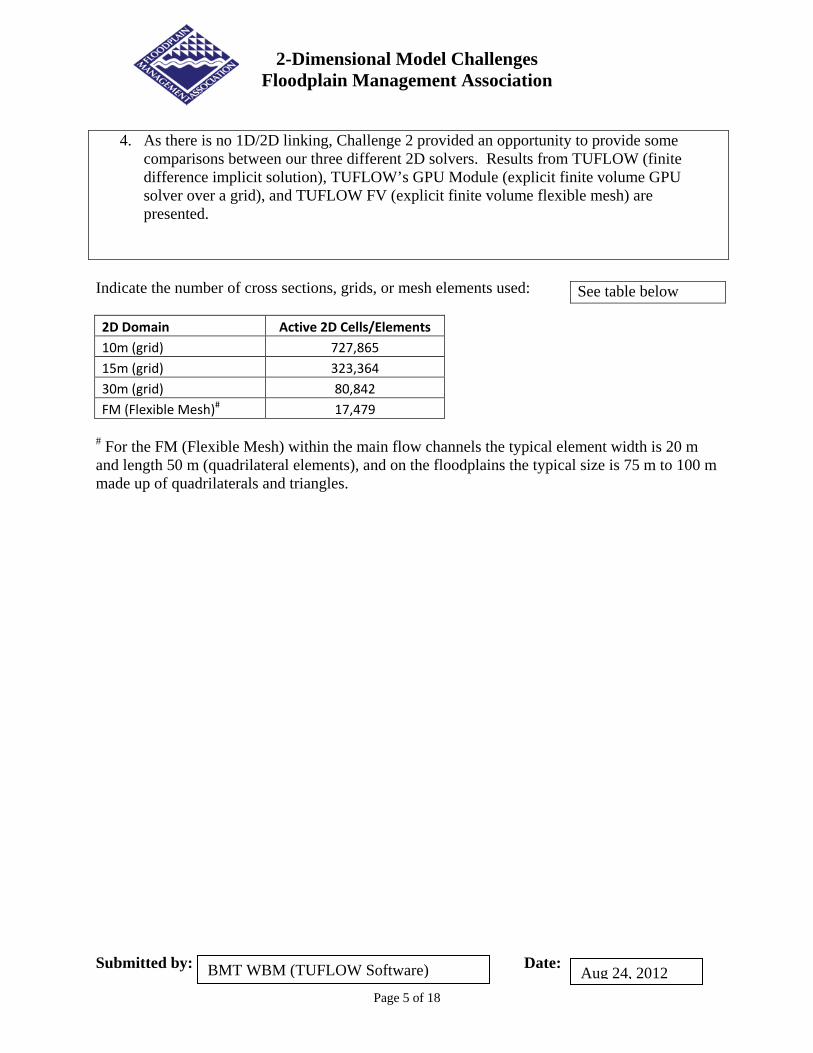
4. As there is no 1D/2D linking, Challenge 2 provided an opportunity to provide some comparisons between our three different 2D solvers. Results from TUFLOW (finite difference implicit solution), TUFLOW’s GPU Module (explicit finite volume GPU solver over a grid), and TUFLOW FV (explicit finite volume flexible mesh) are presented.

Indicate the number of cross sections, grids, or mesh elements used: 2D Domain Active 2D Cells/Elements 10m (grid) 727,865 15m (grid) 323,364 30m (grid) 80,842 FM (Flexible Mesh)# 17,479

# For the FM (Flexible Mesh) within the main flow channels the typical element width is 20 m and length 50 m (quadrilateral elements), and on the floodplains the typical size is 75 m to 100 m made up of quadrilaterals and triangles.

See table below


Submitted by: Date:

Page 6 of 18


Describe the processes used to assemble your computational domain, execute it, and post process it into floodplain limits files. Indicate anything else you want us to know about your data and methods: TUFLOW Fixed Grid Model The TUFLOW model directly reads the provided ESRII ASCII DEM raster format, to set the extent of the computational domain and interpolate elevations at the 2D cell centers, mid-sides and corners. The boundary locations were digitized in GIS layers. The provided GIS land use layer was directly read for assigning roughness values. Simulation results were viewed using SMS and GIS software. Calibration high water marks were loaded into a GIS layer and displayed within the GIS mapping to easily view the calibration performance of the model. TUFLOW’s 3D surfaces of peak water levels and depths were imported into the GIS to generate flood extent outlines. TUFLOW FV Flexible Mesh Model The approach taken to develop the TUFLOW FV Flexible Mesh model was:

1. Using the SMS software with DEM shaded contours as a guide, develop mesh map (creating polygons of specific areas in the model that had a specific mesh design and resolution). The design was such that elements follow bathymetric contours and likely flow directions. Also ensure that narrow flow channels are well resolved and elements lie along center of flow channel.

2. Create mesh, automatically generating geometry (z) values from the DEM. 3. Setup input files, consisting of one input file and 3 boundary condition time series (csv

files). 4. Run simulation on Dell Laptop 64 bit Intel i7 2.8 GHz CPU. 5. Several simulations performed with varying Manning’s friction applied. 6. Within SMS, load shape file with high water marks and point inspect model results of

maximum water level. Export to Excel, convert to feet. 7. Export 3D water level and depth surfaces into GIS to produce maximum flood extent

polygons. Discussion on Calibration Exercise Given the short timeframe for undertaking the Challenge models, only a limited number of simulations were carried out to develop an understanding of the flood behavior and sensitivity of varying parameters. The results of these simulations are discussed below, some of which are provided in the ftp download. Simple Manning’s n / Topography Test The initial runs were carried out using the same Manning’s n over the entire model over a coarse resolution grid and flexible mesh. These runs were carried out using TUFLOW and TUFLOW GPU (30m grid), and TUFLOW FV (flexible mesh) models.


Submitted by: Date:

Page 7 of 18


The topography for these runs did not include any special provision for incorporating the levee and road embankments. The elevation sampling of the DEM was simply based on inspecting the DEM at the models’ elevation points. At this stage no 3D breaklines along the embankment crests were used to ensure the crest of the elevation was correctly represented by the models’ elevations. The Manning’s n used for the results provided was 0.035, which seems to give a reasonable first pass reproduction of the high water marks. A value of 0.035 is consistent with the global n value that would typically apply to this study area. Also of interest is the comparison between the three different 2D solvers TUFLOW, TUFLOW’s GPU Module and TUFLOW FV (all three use a different solution technique). There is generally good agreement between all three schemes. A high resolution .jpg image is provided in the ftp downloads for viewing the HWMs and results of these three simulations. Open “Images\FMA C2.n0.035.HWM All 2D Solvers.jpg” and zoom in and pan around to easily view the flow patterns (velocity arrows), water level contours every 0.2m (blue lines), depths (blue shading) and high water marks (red is the recorded value, light blue is TUFLOW, black is TUFLOW GPU and yellow is TUFLOW FV). NLCD Land Cover and Embankment Crests Included Additional simulations were carried out using TUFLOW that included the NLCD Land Cover GIS layer, and 3D breaklines of the levee and road embankments visible in the DEM and aerial photo. This scenario (we envisage) would probably be representative of the present day conditions, and not representative of the 1964 flood event conditions. The NLCD GIS layer was read directly by TUFLOW and Manning’s n values assigned to the different land covers as tabulated below. The water/river n value of 0.02 is considered at the lower end of typical n values for rivers based on numerous 2D model calibrations. Typically for the lower reaches of coastal rivers the in-bank n value is 0.022 to 0.025 with an acceptable range considered to be (0.02 to 0.03). In upper reaches, away from tidal influences, n values tend to be higher (0.025 to 0.04) for perennial rivers. Possible reasons for the low n value could be due to the river bathymetry accreting since 1964 (we assume the bathymetry provided is based on more recent surveys), or the inflows maybe high.


Submitted by: Date:

Page 8 of 18


The n values used are presented in the table below.

Material ID Manning’s n Description 11 0.04 ! Dummy Open Water - overwritten by digitised polygon 21 0.05 ! Developed 22 0.08 ! Developed 23 0.1 ! Developed 24 0.2 ! Developed 31 0.03 Barren Land (Rock/Sand/Clay) 41 0.05 Deciduous Forest 42 0.05 Evergreen Forest 43 0.06 Unknown 52 0.1 Shrub/Scrub 71 0.1 Grassland/Herbaceous 81 0.04 Pasture/Hay 82 0.05 Cultivated Crops 90 0.1 Woody Wetlands 95 0.1 Emergent Herbaceous Wetlands

101 0.02 Water / sand / silt The NLCD land cover provided a poor representation of the in-bank river section when compared with the DEM and aerial photography. The river section was therefore digitized to replace the NLCD representation in the river. A general comment overall was that the NLCD land cover was not always in agreement with the aerial photo and somewhat poor in its accuracy and resolution. For the levee and road crests, GIS breaklines were digitized along the crests, and elevations sampled from the DEM. Ideally, ground surveys of these hydraulic controls would be available to ensure the crest is accurately modeled. TUFLOW reads the GIS breaklines and interpolates the crest elevation to the nearest 2D cell elevations to ensure the embankment height is correctly modeled. In general the comparison with the high water marks tends to be higher overall, but the distribution of flow has improved with less water travelling to the southern tidal entrance. In a few areas it is worse such as in the images below. In the images the red values are the 1964 HWMs, and the black the calculated peak levels. In these areas the presence of the embankments has a strong influence on the calibration results. To test this influence a further scenario removing two critical embankments was carried out as discussed further below.


Submitted by: Date:

Page 9 of 18



Submitted by: Date:

Page 10 of 18



Submitted by: Date:

Page 11 of 18


Removal of Major Embankments Scenario To test the effect of completely removing the embankments in the images above, the 15m and 30m TUFLOW models were used. Initially the 30m model was run as this is a quick running model so good for an initial sensitivity tests. The embankments were removed by digitizing the polygons shown in grey in the images below, and using TUFLOW’s Z Shape functionality that creates TINs within the polygons whose perimeters are merged with the surrounding ground levels to erase the embankments. This is a very quick process to do and setup (about 5 minutes in this case), and there is no need to rework the original DEM. The images below for the initial 30m grid run show the levels at the high water marks with and without the embankments at the two locations previously discussed. The red values are the 1964 HWMs, the blue values the without embankments scenario and the black values in brackets for the with embankments case previously discussed. An improvement in the calibration results tends to result. The 15m simulation provided an even better calibration, and gives the best overall performance of all simulations carried out. The maximum flood extent layer is provided in the ftp download for this simulation. In conclusion, we would surmise that some of the key embankments within the study area either did not exist at the time of the 1964 event or were of a lower height or configuration. It would be interesting to know the answer!


Submitted by: Date:

Page 12 of 18



Submitted by: Date:

Page 13 of 18



Submitted by: Date:

Page 14 of 18


Describe the “Challenges” you encountered in preparing this floodplain analysis and in mapping the flood limits: The data was much easier to work with than the first challenge! No unexpected “challenges” for Challenge 2, but it is worth noting the challenges that arise in calibration exercises. Sometimes there is an expectation that models should be able to reproduce recorded levels to within a very small tolerance. In these situations there needs to be a good understanding/appreciation by both the client and the modeler of the uncertainties and reasons for discrepancies; and the acceptable tolerances between the modeling and recorded observations accordingly set. Are Manning’s n Values the Same for 1D and 2D models? Generally Manning’s n values are very similar for 1D and 2D schemes. Where there is rapid changes in flow direction and magnitude (eg. at a structure, sharp bend or embankment opening), fully 2D schemes will simulate energy losses associated with the change in flow patterns, whereas 1D schemes either require user specified energy losses (eg. a structure) or artificially increasing Manning’s n. In these situations 1D schemes may utilize higher Manning’s n values than 2D schemes. Conversely, 2D schemes typically apply no side wall friction, so if there is significant wall friction a 2D scheme may require a slightly lower Manning’s n than a 1D scheme. Calibration Challenges Key challenges to note when calibrating are discussed below (this is not an exhaustive list but is a starting point!):

1. Recorded levels can themselves be quite uncertain. They should preferably be rated as to their accuracy and the type of flood mark noted with the recording. For example, a water mark in the wall of a house is a reliable, accurate mark of the peak water level; while a debris level is simply an indication that the flood was at least this high (debris marks may not be at the peak of the flood). Scanning through the high water marks in this study would indicate some inconsistencies. For example, in the northern end of the study area the 5.35 HWM in the image below is upstream of the 5.66 HWM. Either the 5.35 is low and/or the 5.66 is high. If the accuracy of the HWMs can’t be established, then as a generalization, the modeler should err on the high side in case the flood mark was not recorded at the flood peak.


Submitted by: Date:

Page 15 of 18


2. The modeler should NOT adopt unrealistic parameter values (eg. excessively low or high Manning’s n values) for the sole purpose of achieving a good calibration. It is invariably the fact that there are other uncertainties causing the discrepancy when unrealistic Manning’s n values are used. Unrealistic Manning’s n values or other parameters (eg. high eddy viscosity) distort the results and are a sure sign that there is something else wrong.

3. Levees, roads, railways and other embankments can have a major influence on the flood

behavior. Those embankments that overtop should be ground surveyed along their crests and the crest height correctly represented in the model’s elevations. Often for calibration events the height or presence of the embankments is not known accurately and this needs to be taken into account in the ability of a model to reproduce flood marks.

4. The inflows to a model for historical floods often have a high degree of uncertainty, and are the most common reason for a poor calibration. The precise distribution spatially and temporally of the rainfall is not known (sometimes there is little or no rainfall data), and/or the rating curve at a model boundary has significant uncertainties. The significant uncertainties associated with developing model inflows should be understood and appreciated by modeler and client. Ideally, one or more recorded hydrographs would be available to the modeler to verify that the model can reproduce the shape and timing of the flood. If a hydrologic model is being used to generate the inflows, then the calibration exercise should be a joint exercise in calibrating both the hydrologic and hydraulic models.


Submitted by: Date:

Page 16 of 18


5. Inaccurate topography has become less of an issue in recent years with the advent of more accurate aerial surveys. However, the bathymetry of the main flowpaths, and storage capacity of floodplain backwaters, needs to be accurately represented if the model is to have any chance of reproducing flood marks. If these areas have permanent water and/or dense vegetation, the aerial surveys are still incapable of accurately surveying them, so other forms of survey maybe required. If accurate surveys are not available for these areas, this adds to the uncertainty in the modeling and the ability of the model to reproduce historical flood events. There is also the issue of using contour data instead of the raw terrain data to create the DEM as highlighted in our Challenge 1 discussion.

6. Structures are often poorly represented due to lack of data. For example, in the aerial

photograph below for Challenge 2 there appears to be some structures (which has two calibration points in the vicinity). However, with no details provided, the structure below can only be modeled as a simple opening in the embankment with no allowance for bridge decks, etc.


Submitted by: Date:

Page 17 of 18


Estimate computation time required for the analysis execution: __:___:__:__ DHMS

2D Model Typical Run time (dd:hh:mm:ss) CPU Cores Used / GPU TUFLOW 15m Grid 00:04:15:00 1 Core, 3GHz TUFLOW 30m Grid 00:00:25:00 1 Core, 3GHz

TUFLOW FV Flexible Mesh 00:00:50:00 8 Cores, 2.8GHz TUFLOW GPU 10m Grid 00:01:43:00 NVidia Tesla C2075 TUFLOW GPU 15m Grid 00:00:30:00 NVidia Tesla C2075 TUFLOW GPU 30m Grid 00:00:05:00 NVidia Tesla C2075

Challenge 2 Model Results:

I am providing a shapefile containing the maximum flood inundation area which occurred in my model

I am providing an Excel Spreadsheet containing a comparison to the high water marks

Notes: (Please provide any feedback you would like us to consider on this Challenge Model. You could explain your element size selection, N Value selection, model type/software selection or anything else you would like us to know about how you assembled this model) Should further output be required from any of the simulations, please don’t hesitate to contact us. TUFLOW Fixed Grid Models Please refer to discussions above for feedback/explanations. In summary, the TUFLOW 15m No Embankments simulation provided the best calibration (the shape file for the maximum inundation area for this run is included in the ftp download). TUFLOW FV Flexible Mesh Model Given the short timeframe, selection and adoption of approach was based on minimizing preparation time. This approach could be interpreted as a “rapid solution” approach, providing preliminary advice for floodplain managers. The cell sizes in the main river channels were chosen to allow between 5 and 10 cells across the channel width. As flow in the main channels is primarily in one direction, cells length were made longer than cell widths in order to optimize computational performance. Cell sizes on the floodplains were chosen to broadly represent overland flow characteristics, without capturing finer resolution features (such as roads, etc). Differing friction values were tested (including a N = 0.022 in the main channels and rougher values on floodplains), however results with a constant N = 0.035 value provided the most accurate model predictions. N values at 0.035 are somewhat higher than anticipated (especially in the main channels), but considered acceptable.


Submitted by: Date:

Page 18 of 18


It could be argued that a more detailed description should be made of hydraulically significant features on the floodplains (roads, etc) and also a more detailed description of overbank friction (according to land use). However, the calibration event occurred in 1964, which questions the validity of the adopted land use, terrain and (potentially) channel bathymetry – such uncertainties may overshadow any adoption of such details in the model application.

To submit your model results, email this completed form to [email protected] and provide FTP instructions for downloading your deliverables in the space below: FTP Location (example: ftp://ftp.somedomain.com): User name for FTP access: Password:


Date post:	12-Dec-2021
Category:	Documents
Upload:	others
View:	1 times
Download:	0 times

2-Dimensional Model Challenges Floodplain Management ...

Documents