2 - Fundamentals of superconductivity - SciTech...

Fundamentals of superconductivity 2C.M. Rey1, A.P. Malozemoff21Energy to Power Solutions (E2P), Knoxville, TN, USA; 2AMSC, Devens, MA, USA

2.1 History

In this chapter, the fundamental concepts of superconductor phenomena are introducedto provide a foundation for the remaining chapters on high-temperature superconduc-tor power equipment. The discussion focuses on type I and type II superconductors,their corresponding magnetic behaviors, low-temperature superconductors, andhigh-temperature superconductors. The chapter is based on publications byA.C. Rose-Innes, E.H. Roderick, and C. Kittel, supplemented by significant newermaterial arising from the novel properties of high-temperature superconductors.

In the early 1900s, soon after Kamerlingh Onnes had discovered how to liquefy he-lium, he began an investigation concerning the electrical resistance of very pure metalsat low temperatures. At that time, it was unknown how the electrical resistance wouldbehave at very low temperatures. Predictions ranged from the electrical resistancecontinuing to linearly decrease with temperature toward zero, leveling out at someresidual resistance value, or starting to increase at some point due to other electron scat-tering mechanisms. One of the purest metals available at that time was mercury. In1911, Kamerlingh Onnes was measuring the electrical resistance of pure mercury asa function of temperature when he discovered that the mercury’s resistance suddenlydropped to zero below 4 K (De Bruyn Ouboter, Van Delft, & Kes, 2012; KamerlinghOnnes, 1911). Figure 2.1 shows a reproduction of the electrical resistance versus tem-perature plot for pure Hg as measured by Kamerlingh Onnes. He realized that below4 K the mercury entered a new state, which he called “supraconductivity” (De BruynOuboter et al., 2012). No one had predicted this remarkable and fascinating phenom-enon, which still intrigues many today.

Although many materials were subsequently discovered to show the phenomenonof superconductivity at sufficiently low temperatures, it was assumed for many yearsthat only one type of superconductor existed. Only much later was it realized thattwo quite distinct types of superconductors exist. The two types of superconductorshave many properties in common, but their most distinguishing differences show upin their behavior in applied magnetic fields. The type I superconductors (formerlyreferred to as “soft” superconductors), usually elements, lose their superconductingproperties in relatively weak magnetic fields, whereas the type II superconductors(formerly referred to as “hard” superconductors), usually alloys, withstand very strongmagnetic fields before losing their superconducting properties. A few pure elementsare notable exceptions, including niobium, vanadium, and technetium; these aretype II with GinzburgeLandau parameters (see Section 2.8) of k w0.78, 0.82, and

Superconductors in the Power Grid. http://dx.doi.org/10.1016/B978-1-78242-029-3.00002-9Copyright © 2015 Elsevier Ltd. All rights reserved.

http://dx.doi.org/10.1016/B978-1-78242-029-3.00002-9

0.92, respectively (the crossover from type I to type II occurs at k ¼ 1/O2). Each typeof superconductor is sufficiently different and must be treated separately. Discussion ofthe more complex type II superconductivity relevant to power applications is given inSections 2.8e2.11 of this chapter.

2.2 Meissner effect

In 1933,Meissner andOchensenfield (1933) began investigating themagnetic propertiesof type I superconductors. They discovered that if you cool a superconductor in anapplied steady-state magnetic fieldH, then at the superconducting transition temperatureTc, the magnetic field lines are expelled and the superconductor behaves like a perfectdiamagnet with magnetizationM ¼ H/4p orM ¼ H (cgs/mks). This type of magne-tization measurement is sometimes referred to as a field-cooled (FC) experiment and isschematically shown in Figure 2.2 (left). This behavior is far different than a zero-field-cooled (ZFC) experiment and cannot be explained by simply assuming that a supercon-ductor is a perfectly conducting (infinite mean free path) medium. Instead, the Meissnereffect implies that the flux density B inside the material is identically zero (B ¼ 0) for

0.15Ω

10–5 Ω

0.125

0.10

0.075

0.05

0.025

Hg

0.004’00 4’10 4’20 4’30 4’40

Figure 2.1 Reproduction of the original plot of the electrical resistance of Hg versustemperature by Kamerlingh Onnes (1911).

30 Superconductors in the Power Grid

temperatures below Tc. Hence, B ¼ H þ 4pM or B ¼ m0(H þ M) ¼ 0 (cgs/mks), wherem0 ¼ 4p 107 Henries/meter is the permeability of free space. If the superconductorwere simply a perfect conductor with infinite conductivity ðs ¼ NÞ and were cooledbelow Tc in the presence of a steady-state magnetic field H, there would be no magneticflux expulsion (B ¼ 0) at Tc because there was no time varyingmagnetic field dH/dt. Theperfect conductor cooled in a background steady-state magnetic field would simply passthrough Tc as if nothing happened. If, on the other hand, a perfect conductor were cooledin zero magnetic field and subsequently a magnetic field were applied (i.e., dH/dt > 0),the perfect conductor would repel flux. This type ofmagnetization experiment is referredto as ZFC and is schematically shown in Figure 2.2 (right). Thus, the perfect diamagne-tism observed from the Meissner effect with the FC magnetization experiment is a truesignature of superconductivity. Of course, all of these descriptions should be qualified bythe fact that a thin layer (characterized by a magnetic or London penetration depth) at thesurface of the superconductor does admit magnetic flux, as will be explained below.

(a)

(b)

(c)

(d)

(e)

(f)

(g)

(a)

(b)

(c)

(d)

(e)

(f)

(g)

Roomtemperature

Lowtemperature

Lowtemperature

Cooled Cooled

FC

Superconductor Perfect conductor

RoomtemperatureHa = 0

Ha

B 0

Cooled ZFC Cooled

B 0 B 0 B 0

Ha Ha Ha

HaHa = 0Ha

Figure 2.2 Schematic behavior of applied field Ha and magnetic flux density B in field-cooled(FC) and zero-field-cooled (ZFC) experiments on a type I superconductor and non-superconducting material with perfect conductivity. While the ZFC experiment (a / b),followed by application of a field Ha (c) and then removal of the field (d), does not distinguishbetween the two types of materials, the true signature of conventional superconductivity is perfectdiamagnetism, as demonstrated by the FC experiment (path e/ f/ g, cooling of the sample in afield and then removal of the field) known as the Meissner effect. Magnetic flux is excluded fromthe interior of the specimen (B ¼ 0) by supercurrents flowing within the penetration depth at thesurface in the presence of Ha.Adapted from Rose-Innes and Rhoderick (1978, pp. 18 and 20).

Fundamentals of superconductivity 31

2.3 London equations and magnetic penetration depth

In 1935, the London brothers (London & London, 1935) were able to mathematicallydescribe the Meissner effect by assuming that the current density J in the supercon-ducting state is directly proportional to the vector potential A of the local magnetic fieldB, where B ¼ V A (in the London gauge, V$A ¼ 0). The London equation is givenby J ¼ 1=ð4pl2LÞA or J ¼ 1=ðm0l2LÞA (cgs/mks), where lL has the dimensions oflength.

Under static conditions, one of Maxwell’s equations (Ampere’s law) reduces toV B ¼ 4pJ or V B ¼ m0J (cgs/mks). By taking the curl of both sides, thisequation reduces to V2B ¼ 4pV J or V2B ¼ m0V J (cgs/mks). By combiningthis equation with the curl of the London equation, we obtain V2B ¼ B=l2L. The so-lution of this equation is a flux density B, which decays exponentially with distancefrom the external superconductor surface. In a one-dimensional, semiinfinitesuperconducting medium occupying the positive side of the x-axis, the solution tothis equation for the magnetic flux density inside this medium would be B(x) ¼ B0exp(x/lL), where B0 ¼ m0H is the parallel field at the plane boundary (e.g., seeKittel, 1986). In this example, lL measures the distance at which B(x) has fallento 1/e of its initial value, which is known as the magnetic or London penetration depth.

2.4 Critical currents in type I superconductors

A type I superconductor, by definition, is a material that exhibits perfect flux expul-sion in its interior. Physically, the Meissner effect arises because resistanceless cur-rents flow on the surface of the superconductor to exactly cancel B throughout thevolume of the specimen. Thus, if the applied field H is increased, the surface shieldingcurrent will also increase to keep B ¼ 0 inside the specimen. There is, however, anupper limit to the magnitude of surface (within a distance of lL) shielding currentsthat a type I superconductor may sustain. The limiting magnetic field is known asthe critical magnetic field Hc and the corresponding current density is known as thecritical current density Jc. The critical current density may be expressed in terms ofthe critical field by using the curl of the London equation—namely,

V J ¼ ð1=4pl2LÞB or V J ¼ 1

m0l2L

B (cgs/mks). This equation relates

the supercurrent density J to the magnetic flux density B at any point in thesuperconductor.

An inverse to this effect exists. In the absence of an external field, the self-fieldgenerated by the transport current flowing at the surface must not exceed a criticalmagnetic field. If the self-field exceeds this critical field, the superconductor willreversibly pass from its superconducting state to its normal state. This is known asthe Silsbee criterion (Silsbee, 1916). For a type I superconductor with a reversiblemagnetization (see Section 2.5), the Silsbee criterion represents the maximum currentdensity Jc that a type I superconductor can carry before returning to the normal(nonsuperconducting) state. This criterion for Jc holds true for many of the (pure)


elemental superconductors and is quite low, making type I materials not suitable forelectrical power applications requiring high transport currents.

2.5 Magnetization in type I superconductors

A type I superconductor (formerly known as a “soft” superconductor) will exhibit aMeissner effect (i.e., perfect diamagnetism, B ¼ 0) when subject to an applied mag-netic field, independent of whether the material was cooled in zero field (ZFC) or infield (FC), making the material magnetic history independent. This “perfect diamag-netic” response is a reversible thermodynamical process, and the principles of thermo-dynamic phase transitions must apply.

The energy difference between the normal and superconducting state may bedetermined as follows. Consider a long, thin rod with a long axis in the direction of H.This will allow demagnetizing effects caused by the fringing fields at the ends of the spec-imen to be neglected.When anymagnetic material is placed in a magnetic field, its Gibbsfree energy per unit volume G changes by an amount DGðHÞ ¼ RH

0 MdH orDGðHÞ ¼ m0

RH0 MdH (cgs/mks). For a type I superconductor in an applied field,

M ¼ H/4p or M ¼ H (cgs/mks), and the Gibbs free energy increases by H2/8p orm0H

2/2 (cgs/mks). The normal state of a superconductor is commonly only slightly mag-netic and acquires no appreciable change in its free energy. Thus, if H is increased suffi-ciently, the superconductor will reversibly change from its superconducting state to itsnormal state. This change will occur when Gs(T,H) > Gn(T,0) or Hc

2/8p > [Gn(T,0) Gs(T,0)] or m0Hc

2/2 > [Gn(T,0) Gs(T,0)] (cgs/mks). For a type I superconductor, themaximummagneticfield strength that can be applied to a superconductor, if it is to remainin its superconducting state, is the thermodynamic critical field Hc, where Hc(T) ¼ 8p[Gn(T,0) Gs(T,0)]

1/2 or Hc(T) ¼ 2m0[Gn(T,0) Gs(T,0)]1/2 (cgs/mks). A typical

magnetization curve for a type I superconductor is shown in Figure 2.3.

Applied field

Hc

Hc

M

+

–Type-1

0

Figure 2.3 Typical M versus H curve for a type I superconductor. Note the complete magneticflux exclusion (B ¼ 0 or M ¼ H) and the abrupt reversible transition at H ¼ Hc.Adapted from Kittel (1986, p. 324).


The critical magnetic field of a superconductor is found to vary with the tempera-ture. As the temperature is lowered, this value increases. Likewise, as the temperatureis increased, the value of Hc(T) decreases to zero at Tc. The temperature dependence ofHc(T) is given by the general expression Hc(T) ¼ Hc0 [1 (T/Tc)

a], where Hc0 is themeasured critical magnetic field at zero temperature (T/0) and a has a theoreticalvalue of 2. In practice, a is an experimentally fitted parameter typically close to 2for most superconductors. Tc and Hc are intrinsic properties of a superconductor,and using the given temperature-dependent properties, Hc can be calculated for anyvalue of temperature below Tc. Similarly, the temperature dependence for the criticalcurrent density is given by Jc(T) ¼ Jc0 [1 (T/Tc)

b], where Jc0 is the critical currentdensity at zero temperature and b is experimentally fitted with values typically closeto unity.

2.6 Intermediate state

2.6.1 Demagnetizing coefficient

The demagnetizing magnetic field is the magnetic field Hd generated by the magneti-zation M within the magnet. The total magnetic field in the magnet is a vector sum ofthe demagnetizing field and the magnetic field generated by any free or displacementcurrents. The term demagnetizing field reflects the tendency of this field to reduce thetotal magnetic moment of the specimen. The demagnetizing field can be very difficultto calculate for arbitrarily shaped objects, even in the case of a uniform magnetizingfield. For the special case of ellipsoids, which includes objects such as spheres, longthin rods, and flat plates, Hd is linearly related toM by a geometry-dependent constantcalled the demagnetizing factor n. For a long thin rod placed in a uniform magneticfield along its long axis, the demagnetizing factor approaches zero. For a sphere placedin a uniform magnetic field, the demagnetizing factor is 1/3; for a flat plate withmagnetization perpendicular to the plane, it approaches unity. The result is that incertain sample shapes, the demagnetizing field can concentrate the magnetic field linesin certain localized regions of the specimen relative to the bulk sample. These shape ordemagnetizing effects must be considered and accounted for in superconductingapplications operating in the presence of magnetic fields.

Consider now the magnetic properties of a type I superconductor with a nonzerodemagnetizing factor n. To keep the mathematics as simple as possible, a sphericalgeometry will be assumed. A demagnetizing factor n assigned to any superconductingbody is defined by n ¼ (Hi H)/M, where H is the applied field and Hi is thefield strength inside the specimen. The value of n ranges from 0/4p or 0/1(cgs/mks). The effective value of B inside such a body is the total flux passing throughthe specimen divided by its maximal cross-sectional area. However, we must nowconsider that to satisfy the electromagnetic criteria when the applied field is suffi-ciently high, the sample will need to break up into domains of normal and supercon-ducting regions, each having the respective areas Xn and Xs. This is called theintermediate state, which must be distinguished from the mixed state (discussed later


for type II superconductors). In a type I superconductor, B ¼ 0 inside any supercon-ducting region (except in the magnetic penetration depth at the surface). For thesample, B is zBn, where Bn is the local flux density in the normal regions, andz ¼ Xn/(Xn þ Xs) is the fractional cross-section which is in the normal state. The localmagnetic field in all regions of the specimen should not exceed the critical magneticfield Hc or the sample can enter this intermediate state with alternating regions ofnormal and superconducting material.

2.6.2 Surface energy

To qualitatively understand many of the magnetic properties of superconductors, wemust introduce the concept of a surface energy that can exist between the normaland superconducting (n/s) phases. The Gibbs energy will now be either increased ordecreased by the additional contribution coming from the surface energy. The magni-tude of the surface energy per unit area depends on the material and its correspondingrelevant length scales of the magnetic penetration depth lL and its coherence length x,which will be discussed in the next section. If the surface energy is positive, the Gibbsenergy is minimized by decreasing the area at the n/s boundary. The converse is true fora material with a negative surface energy, where energy is released on forming an n/sboundary. If the Gibbs energy is lowered by forming an n/s boundary (negative surfaceenergy), then the superconductor will want to split into a large number of n/s interfacesto increase the area at the n/s boundary. This will occur even in the absence of a demag-netizing field at fields <Hc.

2.7 Coherence length

2.7.1 History

Pippard (1953) introduced the concept of a coherence length x while studying thenonlocal generalization of London’s equation. This concept of a coherence lengthwas later used to explain the origin of the surface energy at the normal/superconduct-ing boundary. Pippard reasoned that the density ns of the highly ordered super-electrons cannot change rapidly with position. Instead, ns can only change appreciablywithin a distance he called the coherence length. Loosely speaking, the coherencelength can be viewed as the spatial distance over which the superconducting state(i.e., electroneelectron pairing length scale) can exist.

2.7.2 Magnitude

Pippard demonstrated how the concept of a coherence length may be derived fromthermodynamic principles; however, its magnitude can be estimated by using an un-certainty principle argument. The electrons that can play a role in the superconducti-vity have an energy within wkTc of the Fermi energy, where k ¼ 1.38 1023 J/K isBoltzmann’s constant. The momentum range of these electrons is Dp wkTc/vF, where


vF is the Fermi velocity. Using the uncertainty relation, one determines the uncertaintyin the real space position, which has a characteristic length x0 ¼ ahvF/2pkTc where a isa numerical constant of order 1, to be determined for each superconducting material,and h ¼ 6.63 1034 J-s is Planck’s constant. For pure elemental type I superconduc-tors, the coherence length is quite large: x0 w1000 nm. For high-temperature super-conductor (HTS) materials, the coherence length is quite short: x0 w1e4 nm intheir ab-plane and less than 1 nm along the c-axis (see below).

2.7.3 Dependence on purity

An intrinsic characteristic of the coherence length and the penetration depth is theirdependence on the purity of the material or essentially the electron mean free path‘. The coherence length in a perfectly pure material (denoted as x0) is larger than inan impure specimen (denoted as x). We define both a “clean” and “dirty” limit of asuperconductor, which depends on the magnitude of ‘ and x0. In the clean limit,‘>>x0, but in the dirty limit, ‘<<x0. When a superconductor is very impure or inthe dirty limit, then x w(x0‘)

1/2 and l wlL (x0/‘)1/2 so that l/x wlL/‘. Because x0

is so small in HTS materials, they tend to be in the clean limit.

2.8 Type II superconductors

2.8.1 History

For many years, anomalous magnetic behavior—that is, behavior inconsistent with theunderstanding of type I superconductors—was observed in superconducting alloysand impure metals. These anomalies were ascribed to impurity effects. In 1957,Abrikosov (1957) published a groundbreaking paper explaining these anomalies asinherent features of another type of superconductor with a radically different set ofproperties. This other class of superconductivity became known as type II supercon-ductivity (or, formerly, “hard” superconductors).

2.8.2 GinzburgeLandau parameter

The criterion as to whether to classify a material as either type I or type II can beexplained in terms of the surface energy—that is, whether the surface energy is positiveor negative. Both x and l provide separate contributions to the surface energy by raisingor lowering the free energy of the superconductor relative to the normal(i.e., nonsuperconducting) region. Due to the presence of the ordered super-electrons,the free energy density of the superconducting state is lowered by an amount Gn e Gs.However, because the superconducting region has acquired a magnetization whichcancels B inside, there is a positive magnetic contribution to Gs equal to Hc

2/8p orm0Hc

2/2 (cgs/mks). At the boundary of the normal/superconducting phases, the degreeof electron pair order rises over a distance x; however, counteracting this is the increase


in Gs stemming from the magnetic contribution, which rises over a distance of l. Thus,the order introduced by entering the superconducting state decreases the free energyGs;however, because the material transitions from essentially a nonmagnetic state to a per-fect diamagnet with relative permeability mr ¼ M/H ¼ 1, the presence of a magneticfield increases the free energy Gs.

Abrikosov developed the theory of type II superconductors (Abrikosov, 1957)based on the famous phenomenological theory of Ginzburg and Landau (1950).In this theory, the ratio of l/x, defined as k, determines the value of the surface energy.If k is less than 1/O2, then the surface energy is positive; if k is greater, the surfaceenergy is negative.

2.9 The mixed state: Hc1 and Hc2

2.9.1 Quantized flux lines or vortices

If the surface energy between the normal and superconducting phases is negative, thenit is energetically favorable for the superconducting body to split into a large number ofnormal regions whose boundaries lie parallel to the applied magnetic field. This iscalled the mixed state. In the normal regions, the material is no longer superconducting(i.e., perfect diamagnetism) and the external applied magnetic field can penetrate thesuperconductor in this region. The extent of the magnetic field decays over a distanceof lL (see Figure 2.4, left). The normal regions form in the shape of cylinders (oftenreferred to as normal cores), threading the bulk of the superconductor. The cylindricalshape is preferred because of its high ratio of surface area to volume. The normal coreshave a very small radius (wx) because of their high ratio of surface area to volume.The magnetic flux in the normal core, having the same direction as the external appliedmagnetic field, is generated by a vortex of persistent supercurrent that circulatesaround the normal core with a sense of rotation that is opposite to the bulk diamagneticresponse of the superconductor (Figure 2.4, middle). The radius of the vortex is oforder l, and because l is much larger than x in HTS materials, the current vortex

Figure 2.4 Structure of a flux line or vortex in a Type II superconductor, with contributionsfrom positive surface energy with corresponding length scale l and negative surface energy withits corresponding length scale x. In the far left, the external applied magnetic field penetrates thebulk of the superconductor as a flux line carrying a flux quantum, which is maintained by acirculating persistent current J(r). In the middle left, the magnetic field created by the persistentcurrent J extends out a radius l. In the middle right, the normal core extends a radius x with thehole in the number ns of superconducting electrons also extending a radius x (far right).


spreads far outside the tiny normal core. The value of magnetic flux threading thenormal core is quantized in discrete units given by F0 w2.07 107 G cm(Kittel, 1986).

In this chapter, we use the terms flux lines and vortices, and occasionally fluxons orfluxoids, interchangeably to denote these remarkable quantized linear structures thatcan thread type II superconductors in their mixed state.

The picture of the cylindrical normal core is only approximate; however, because itdoes not have sharp and fixed boundaries. As discussed in Section 2.7, the number nsof superconducting electrons falls over a distance wx (Figure 2.4, right). The conceptof the normal core with the applied magnetic field penetrating its center is extremelyimportant in the design and fabrication of practical superconductors, for if the normalcores move or are set in motion, this can result in a time-changing magnetic flux. FromMaxwell’s equations, a time-changing magnetic flux in turn results in an electric fieldand hence unwanted dissipation in the superconductor. Thus, a major task in process-ing practical superconductors is to find ways to pin the flux lines in place.

2.9.2 The Abrikosov lattice

The vortex persistent current circulating around the normal core interacts with themagnetic field produced by its neighboring vortices; as a result, the vortices have amutual repulsion force between them. Because of this mutual interaction, the vorticesthreading an ideal (undefected) type II superconductor arrange themselves into aperiodic array at high enough fields, and they have been directly observed by a varietyof decoration or electron microscopy techniques (see Figure 2.5). This periodic array isknown as the fluxon, vortex, or Abrikosov lattice. The energetically most favorableconfiguration for the vortex lattice in an isotropic and perfect Type II superconductoris a triangular close-packed lattice (Abrikosov, 1957). The distance between vortices,known as the vortex lattice parameter a, is often less than 105 cm and is equal to(2F0 /O3B)

1/2. Note that in a few materials the vortex lattice is known to be square,presumably because of intrinsic anisotropy in the material.

The mixed state is bounded by two critical field strengths Hc1 and Hc2. Below thelower critical field strength Hc1, the material is fully superconducting (B ¼ 0), exceptfor the magnetic penetration depth at the surface, and quantized vortices are excludedfrom the bulk. Above the upper critical field strength Hc2, the material is fully normal.

An approximate value for Hc1 can be obtained by considering the value of theGinzburgeLandau parameter k. The mixed state will be energetically favorable ifH ¼ Hcx/l, where Hc is the thermodynamic critical field. This gives a value forHc1 wHc/k. As k increases, the relative ratio of Hc1 to Hc decreases, and with thehigh values of k in HTS materials, Hc1 is very small.

An estimate ofHc2 can be made by examining the properties of x. Recall that x is thelength scale over which superconductivity may rise or fall from the normal state. AtHc2, the normal cores are packed together as densely as x will allow. Each core admitsone quantized unit of flux, F0 w2.07 107 G cm (Kittel, 1986, see Section 2.13);thus Hc2 wF0/2px (Kittel, 1986), where px2 (Kittel, 1986) is the cross-sectionalarea of the normal core.


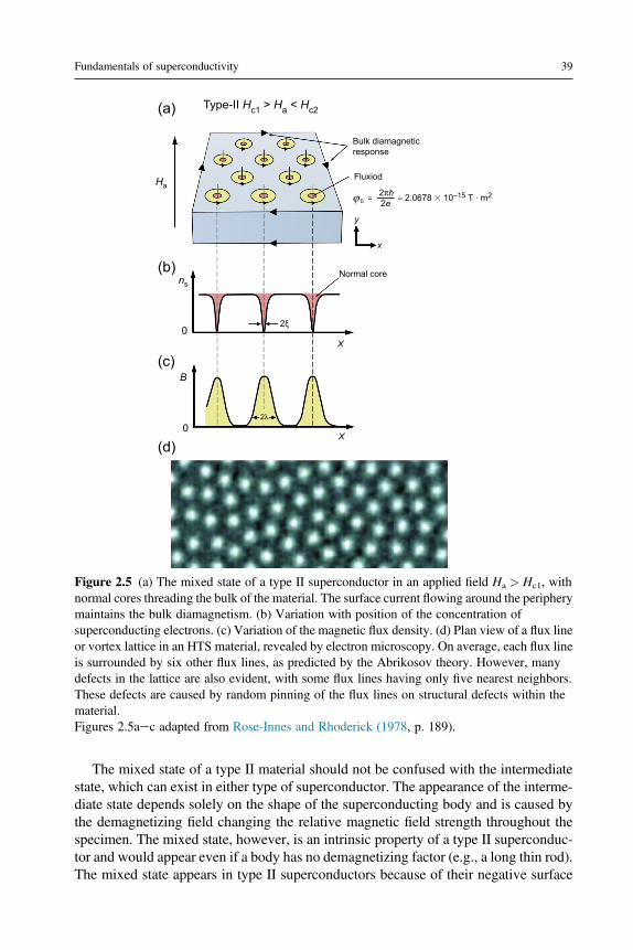
The mixed state of a type II material should not be confused with the intermediatestate, which can exist in either type of superconductor. The appearance of the interme-diate state depends solely on the shape of the superconducting body and is caused bythe demagnetizing field changing the relative magnetic field strength throughout thespecimen. The mixed state, however, is an intrinsic property of a type II superconduc-tor and would appear even if a body has no demagnetizing factor (e.g., a long thin rod).The mixed state appears in type II superconductors because of their negative surface

Type-II Hc1 > Ha < Hc2

Bulk diamagneticresponse

Fluxiod

y

x

2ξ

X

ns

Ha

X

2λ

0

B

0

Normal core

ϕ =2π2e

h ≈ 2.0678 10–15 T ∙ m2

(a)

(b)

(c)

(d)

Figure 2.5 (a) The mixed state of a type II superconductor in an applied field Ha > Hc1, withnormal cores threading the bulk of the material. The surface current flowing around the peripherymaintains the bulk diamagnetism. (b) Variation with position of the concentration ofsuperconducting electrons. (c) Variation of the magnetic flux density. (d) Plan view of a flux lineor vortex lattice in an HTS material, revealed by electron microscopy. On average, each flux lineis surrounded by six other flux lines, as predicted by the Abrikosov theory. However, manydefects in the lattice are also evident, with some flux lines having only five nearest neighbors.These defects are caused by random pinning of the flux lines on structural defects within thematerial.Figures 2.5aec adapted from Rose-Innes and Rhoderick (1978, p. 189).


energy. In addition, the structure of the intermediate state has very coarse features anddimensions that could be visible with the naked eye. The mixed state’s dimensionshave a much finer scale (w105 cm).

2.10 Reversible magnetization in type IIsuperconductors

The magnetic properties of an ideal, nondefected type II superconductor are describedby three regions of applied field. Below Hc1, a type II superconductor behavesidentically as a type I superconductor; that is, it has a perfect Meissner effect withM ¼ H/4p, M ¼ H (cgs/mks). Above Hc1, quantized flux lines or vortices pene-trate into the material, so that B in the material is no longer zero and M decreases.For Hc1 < H < Hc2, the number of vortices and their distribution in the sample aredetermined by the mutual repulsion among the vortices and the magnitude of theapplied field, and an Abrikosov lattice is formed. An electron micrograph of a fluxline or vortex lattice is shown in Figure 2.5d.

As H increases toward Hc2, the normal cores pack closer together, increasing theaverage value of B in the superconductor. Near Hc2, B and M change linearly withH. At the value Hc2, in conventional theory (see Section 2.11 for modifications inHTS materials), there is a discontinuous change in the slope of the magnetizationcurve. Above Hc2, the material is in the normal state, which is virtually nonmagnetic.A typical magnetization curve for an ideal, undefected type II superconductor is shownin Figure 2.6.

Applied field

M 0Hc1 Hc2Hc

Mixed/vortex state

Normal state

Superconductingstate

Type-II

+

–

Figure 2.6 Typical magnetization curve for an undefected type II superconductor. ForH < Hc1,the sample is in the superconducting state exhibiting perfect diamagnetism; for Hc1 < H < Hc2,the sample is in the mixed/vortex state; and for H > Hc2, the sample returns to the normal state.Adapted from Kittel (1986, p. 324).


However, this picture is dramatically changed in HTS materials, where thermalactivation destroys the long-range order of the Abrikosov lattice above a certain temper-ature or magnetic field, creating a huge region of the phase diagram in the HeT plane inwhich the flux lines or vortices exist in a “liquid-like” state. This novel phase diagram,illustrated schematically in Figure 2.13, is discussed in greater detail in Section 2.11.

2.11 Critical currents and irreversible magneticproperties of type II superconductors

Owl explained about flux pinning and creep. He had explained this to Pooh andChristopher Robin once before, and had been waiting ever since for a chance to do itagain, because it is a thing you can easily explain twice before anybody knows whatyou are talking about.(After A.A. Milne, Winnie-the-Pooh, in Blatter, Feigel’man, Geshkenbein, Larkin, &

Vinokur, 1994)

Critical currents and irreversible magnetic properties in type II superconductorsinvolve multiple complicated mechanisms. Unlike Tc, Hc1, and Hc2 which are intrinsicproperties of superconductors, Jc tends to be an extrinsic property controlled by defectsthat are greatly affected by the fabrication process. Furthermore, especially in thenew HTS materials, Jc is affected by thermal activation leading to flux creep and apower-law IeV curve, so that Jc must now be interpreted as a quantity determinedby an arbitrary electric field criterion. The irreversible magnetic properties of type IIsuperconductors are in turn controlled by the critical current density and are explained,at least to a first approximation, by the so-called Bean critical state model (Bean, 1962,1964). This section introduces these complex phenomena in greater, although stillminimal, detail; the full picture can be found in the wonderful reviews by Campbelland Evetts (1972) and Blatter et al. (1994). In particular, thermal activation effectsand flux creep have revolutionized our understanding of the classical theory of super-conductors and have a major impact on properties relevant to applications.

2.11.1 Critical currents and pinning in defected type IIsuperconductors: the T ¼ 0 limit

2.11.1.1 Flux line gradient

Except for the most perfect specimens, the Silsbee criterion (Silsbee, 1916), discussedpreviously, is largely irrelevant when determining the critical current density Jc of typeII superconductors because Jc is overwhelmingly determined by defects. This is fortu-nate because the defect-controlled Jc can be far higher, and current can flow throughthe entire bulk of the material, not just on the surface as in type I materials. The higherJc values enable practical HTS superconductors for electric grid applications.

One can see how defects in a superconductor come into play from Ampere’s law,which in vector notation and mks units is V B ¼ m0J, and in a one-dimensional form


is dB/dx ¼ m0J. Thus, any bulk current flow or current density J must correspond to agradient in B. In a type I superconductor, the resistanceless current only flows on thesurface of the material within a penetration depth lL. However, in a type II supercon-ductor in the mixed state, resistanceless current can flow throughout the bulk if twoconditions are met: (1) flux and hence B can be introduced into the volume of thesuperconducting body so that it is filled with flux lines and (2) there is a gradient inthe flux line density.

However, because the equilibrium state of the flux-line lattice in a perfect undefectedsuperconductor has uniform density (the Abrikosov lattice), the only way to sustain agradient is through defects that pin the flux lines in potential wells, with defects of asize comparable to the coherence length and the normal core of the flux line beingmost effective. The pinning is theoretically understood from the reduced free energyat the defect.

2.11.1.2 Maximum pinning force and critical current density

As current density through a type II superconductor is increased, the flux-line gradientgrows steeper according to Ampere’s law, creating ever-stronger forces to push theflux lines out of their defect potential wells. When that force exceeds the maximumgradient in the potential energy of the well (i.e., the maximum pinning force), theflux lines are pushed out of the well. A crude analogy is a washboard holding marbles;as the washboard tips and the point is reached where no barrier remains, the marblesroll out. At T ¼ 0, this is the point that determines the critical current density Jc. Themaximum pinning force can be written as Fp ¼ Jc B, where B is proportional to thelocal flux line areal density. Thus, the magnitude of the pinning force can bedetermined from a measurement of Jc in the presence of a given average flux levelB. An example of data on an HTS second-generation yttrium barium copper oxide(YBCO) wire is shown in Figure 2.7 with two different concentrations of the impurityZr, which affects the defect concentration in the material through the spontaneousformation of BaZrO3 defect columns during film growth.

2.11.1.3 VeI curve and pinning optimization

If the applied current density exceeds Jc, the flux lines move; thus, by Lenz’s law, theygenerate voltage. The superconductor VeI curve looks like a hockey stick: zerovoltage up to a critical current, and then an abrupt increase in voltage. Such a criticalcurrent is easy to measure. We note that an inhomogeneous distribution of Jc in a ma-terial can smear out this sharp VeI curve, and the right kind of distribution can cause apower law dependence VwIn, which is often observed in superconductors (Warnes &Larbalestier, 1986). Of course, in this case, the power or index value n is expected todepend strongly on the particular inhomogeneity distribution. Here, we discuss anothermechanism for the power-law VeI curve, which arises from flux creep and is partic-ularly relevant to HTS materials.

Given the importance of high Jc in practical applications, it is no surprise that manystudies address both the theoretical determination of Jc for different types of defects, as


well as the experimental optimization of defects to pin the flux lines most strongly andincrease Jc (Blatter et al., 1994; Campbell & Evetts, 1972). It is a complex problembecause interactions between flux lines come into play, causing Jc to be determinedby collective phenomena. Therefore, it is not necessary to pin every flux-line core atan impurity site for all flux lines to remain stationary in the face of a flux-line gradient.

Tremendous progress has been made, both theoretically and experimentally; nowpractical materials, including HTS materials like YBCO, carry huge current densities(Malozemoff et al., 2012). Much of the pinning force in these materials arises fromnaturally occurring dislocations, crystal twin boundaries, stacking faults, chemicalprecipitates, voids, and the like. A significant research and development (R&D) effortalso goes into developing artificial pinning centers, such as patterning defects intosubstrates, which are then replicated in deposited HTS films. A large literature also ad-dresses irradiation by protons, neutrons, and heavy ions—damage from which cansignificantly increase both the magnitude of the pinning force Fp and the number ofthese pinning centers (Civale, 1997; Weber, 2011). Disorder in the location of pinningcenters is a critical factor in determining Fp, leading to the breaking up of the Abriko-sov lattice into the famous Larkin-Ovchinnikov (Larkin & Yu., 1964) and Fulde-Ferrell domains (Fulde & Ferrell, 1964). This creates a veritable “zoology” of differenttypes of glassy behavior, usually referred to as a vortex glass (Blatter et al., 1994).

2.11.1.4 Lorentz force

Another way to understand this phenomenon is in terms of the so-called Lorentz forceper length FL, which acts on each vortex in the presence of bulk current density J. Notethat the locally averaged magnetic induction field B is proportional to the areal flux line

500

450

400

350

300

250

200

150

100

50

00 1 2 3 4 5 6 7 8 9

Magnetic field (T)

Pinn

ing

forc

e (G

Nm

–3)

30 K, B ⊥ Tape

15% Zr

7.5%Zr

Figure 2.7 Pinning force density (GN/m3) versus applied magnetic field at T ¼ 30 K with fieldperpendicular to the plane of YBCO-coated conductor tape. In these chemical vapor-depositedfilms, extra Zr forms columns of BaZrO3, which are strong pinning centers.Courtesy of V. Selvamanickam, University of Houston.


density. Thus, B ¼ nF0, where n is the number of flux lines per unit area and F0 istaken as a vector pointing in the direction of flux lines and hence of B. Then, fromAmpere’s law, one can derive the elegant vector formula:

FL ¼ JxF0 ¼ JF0 sin q (2.1)

The vector relationship follows the right-hand rule, so that the force is perpendic-ular to the plane defined by J and F0. In the scalar form of the formula, q is the anglebetween J and F0; therefore, for applied fields perpendicular to the axis of a wire, thisreduces to FL ¼ JF0. If the pinning force per length Fp is the maximum slope of adefect’s free energy well, the criterion for pinning in the presence of a current densityJ passing through the sample is Fp > FL.

2.11.2 Bean critical state model

2.11.2.1 Magnetic moment and magnetization

The penetration of flux lines into defected type II superconductors gives rise tofascinating and important irreversible magnetic behavior.

It is useful to review the basic definitions of magnetic moment and magnetization.The magnetic momentm is the product of a loop of current I and the area A it surrounds(m ¼ IA). In a ferromagnet, for example, each magnetic atom carries a spin, which iseffectively a loop current. However, because each atom carries the same spin, all thelocal currents, when averaged over many spins inside the material, cancel out and onlya net surface current flows, as shown schematically in Figure 2.8 (left). That surface

FerromagnetSuperconductor

Type-II

Atomic spins Quantizedvortices

Surface current Diamagnetic bulksuper-current

B = 0B=μ0H atsurface

Figure 2.8 Schematic current flows in a ferromagnet and type II superconductor. In theferromagnet, atomic spin currents uniformly distributed cancel out in the interior but create a netsurface current that, when multiplied by the area, gives the magnetic moment. In a type IIsuperconductor, quantized flux lines with their vortex current loops penetrate into the bulk, butwith a density gradient that corresponds by Ampere’s law to a diamagnetic current at the criticalcurrent density. If the external field H is not too high, a region in the center remains screened(B ¼ 0).


current multiplied by the area of the sample determines m, and the magnetization M isjust the magnetic moment m per unit volume.

2.11.2.2 Basic principles of the Bean model: the sand-pileanalogy

Consider now the cross-section of a long rectangular superconductor rod with anapplied field H applied parallel to its axis. For the case of HTS materials, Hc1 is smalland we ignore it in the present discussion. By continuity of the surface field, the fluxline density B at the rod surface must equal m0H. Therefore, flux lines parallel to therod axis enter the superconductor; when viewed end-on, in the cross-section ofFigure 2.8 (right), each flux line is surrounded by a vortex of current, analogous tothe spin current of ferromagnetic atoms. Because this penetration of flux lines intothe material creates a flux gradient, a corresponding current must, by Ampere’slaw, flow perpendicular to the flux lines. Indeed, as can be seen by examining neigh-boring local loops in Figure 2.8 (right), the local currents do not cancel out as in theferromagnet, but because of the flux line density gradient, a net local current flows.This net of the local vortex currents is in fact the physical source of the bulk currentflow in type II superconductors. Furthermore, because flux lines penetrate from allsides, this current flow forms a loop, as indicated schematically by the blue arrowsin the figure. The current flow direction is such as to create a moment opposing theapplied field; in other words, this is a diamagnetic current that effectively shieldsthe sample interior, although not as completely as the Meissner current of a type Isuperconductor.

As long as the average slope dB/dx of the flux front exceeds m0Jc, the Lorentz forceof the current pushes flux lines out of the material’s pinning wells, causing the fluxfront to advance and the flux gradient to decline. This process only stops when theflux gradient dB/dx equals m0Jc, at which point the defect potential wells just balanceout the Lorentz force. If the applied field is increased, once again more flux lines mustenter the material, and the flux front advances until it stabilizes a bit further in, butagain with the same slope m0Jc.

This physical process, with the simple and fundamental insight that the fluxgradient always stabilizes at m0Jc, and with any modifications to the flux configurationinitiated only by applied field changes at the surface, is the essence of the famous Beanmodel (Bean, 1964; Campbell & Evetts, 1972). This model provides a simple andintuitive way to calculate magnetic properties of defected type II superconductors.Another well-known analogy to this irreversible flux penetration process is theso-called sand-pile model. Think of a child’s sandbox with sand added at the edges.Loose and dry sand has a characteristic slope, like a talus slope. As sand is added atthe edge (analogous to increasing the external applied field), the sand advances andonce again stabilizes at the characteristic slope. If sand is removed from the highside of the slope (analogous to decreasing the external applied field), a new slope formswith the opposite inclination and gradually eats in to the original slope as more andmore sand is removed. Once this physical picture is understood, one can begin to applythe model to a tremendous diversity of important situations.


2.11.2.3 Magnetic hysteresis loopof a type II superconductor tape

In the case of Figure 2.8 (right), with the “sand” coming in from all four sides, it isimmediately evident that a kind of “picture frame” configuration develops, as sug-gested by the dashed lines in the figure, surrounding a flux-free region in the center.Let us now consider the case where the width w is much larger than thickness d, sothat the rod looks like a tape. The magnetic properties are then dominated by thetape width; although the ends still play an important role, as this is where the current“turns around,” they can be ignored to a good approximation.

The field and current directions in the tape are shown schematically in Figure 2.9(a),with a set of flux penetration profiles with increasing applied field shown inFigure 2.9(b) as a function of position through the thickness d. From Ampere’s law,it is immediately evident that the distance of flux front penetration from each surfaceis just x ¼ H/Jc. When

Hfullpenetration ¼ Jcd=2 (2.2)

the flux fronts meet at the center, fully penetrating the sample. Because the current nowflows in the volume of the superconductor, to evaluate the total moment, it is necessaryto integrate over all the current loops as a function of their positions from the edge ofthe sample. Equivalently, one can use the basic relationship M ¼ (Bave/m0) e H toderive the magnetization M by averaging over the flux penetration profile B(x).

Calculating M now becomes a simple evaluation of the area between m0H and theflux contour B in Figure 2.9(b). The result forM(H), starting from flux-free material, isas follows:

M ¼ H2Jcd

H; H < Jcd=2 (2.3)

At the full penetration field and above, it is immediately evident from the shadedarea in Figure 2.9(b) that M remains constant at

M ¼ m0Jcd=4; H > Jcd=2 (2.4)

Equation (2.4) shows thatM is proportional to Jc, providing a widely used magneticmethod of determining Jc. Of course, this relation only holds in specific experimentalconfigurations and under adequately high applied fields; therefore, one must make sureproper conditions apply in a given experiment.

When the field is now reduced, the slope of B at the surface reverses as shown inFigure 2.9(c), and accordingly a region of reversed current flow develops near the sur-face. Once the field has been reduced by Jcd, the magnetization M ¼ þm0Jcd/4 is nowpositive and constant for a further reduction of the applied field, as evident from theshaded area in the figure.

The full hysteresis loop is shown schematically in Figure 2.9(d). However, incomparing to experiment, many additional effects need to be taken into account.A key one is the field-dependence of Jc(B), which declines strongly with jBj in most


HTS materials. This creates a peak in jM(H)j near H ¼ 0. HTS materials are also high-ly anisotropic; therefore, the hysteresis loop depends strongly on the direction of H.Demagnetization effects must also be taken into account, such as when the field isapplied perpendicular to the HTS tape plane.

2.11.2.4 Alternating current loss in the Bean model

The alternating current (AC) hysteretic power loss P per volume can be derived fromthe hysteresis loop area as a function of the peak-to-peak applied field Hpep. For the

J

H H

H

H

H

M

–M

+M

B(x)

–Jcd/4

–Jcd/2

+Jcd/4

B(x)

w

d dx

0

dx

0

(b)(a)

(c) (d)

Figure 2.9 (a) Schematic orientations of applied field H and current flow J in a finite length oftape of width w and thickness d. (b) Schematic flux penetration profiles into the thickness of thetape as H is increased, according to the Bean model. (c) Schematic flux profiles as H isdecreased. (d) Schematic hysteretic magnetization loop for the process illustrated in (b) and (c).


simple case in Figure 2.9, at sufficiently high applied AC fields and at a frequency f, theloss is simply as follows:

P ¼ m0JcdfHpp=2; Hpp[Jcd (2.5)

At lower fields, one finds (Bean, 1964; Campbell & Evetts, 1972) that

P ¼ m0H3pp f =12Jcd; Hpp < Jcd (2.6)

These classic Bean model formulas have been widely used in interpreting ACexperiments (see Chapter 5, Section 5.3).

The Bean model has also been applied by Norris (1970) for the case of an ACcurrent in an elliptical or tape-shaped wire. For example, the formula for the ACloss per length of a tape-shaped wire is

P ¼ m0=6p

I2c fF

4; F < 1 (2.7)

where F ¼ Ipeak/Ic, Ic is the critical current of the wire and Ipeak is the magnitude of thepeak current. The Norris formulas are also widely used in studies of wire AC loss(see Chapter 5, Section 5.3).

2.11.3 Critical current in defected type II superconductors atT > 0: flux creep

2.11.3.1 AndersoneKim flux creep theory

The phenomenon of flux creep plays a vastly more important role in HTS materialsthan in the conventional low-temperature metallic superconductors (LTS), primarilybecause of their small coherence lengths x and high anisotropy. This is true even atT ¼ 0 because the HTS coherence length, and consequently also the barrier to fluxline escape from its potential well, have atomic dimensions, opening the possibilityfor quantum mechanical tunneling through the barrier. Such tunneling leads toflux creep at T ¼ 0 and hence the appearance of a slight voltage, even below Jc.This phenomenon has in fact been observed in YBCO (Fruchter et al., 1991).Nevertheless, it is small compared to the much larger flux creep caused by thermalactivation.

At finite temperatures, thermal energy can cause flux lines to hop out of their pinningpotential wells following the familiar Arrhenius activation law. Because the barrieris reduced by the Lorentz force of Eqn (2.1), the J-dependent barrier is, in the simplestmodel (Anderson & Kim, 1964; Malozemoff, 1991; Yeshurun, Malozemoff, &Shaulov, 1996), as follows:

UJ ¼ U0½1 J=Jc0 (2.8)


Then, the rate of decay of a current of density J circulating within a superconductor is

dJ=dtwt10 exp

UJ=kT

(2.9)

where t0 is a hopping attempt time, T is temperature, and k is Boltzmann’s constant.This leads to the famous AndersoneKim formula for flux creep (Anderson & Kim,1964):

JðT ; tÞ ¼ Jc01 ðkT=U0Þ lnðt=teffÞ

(2.10)

where teff is proportional to t0 along with some geometrical factors. The currentdecay is commonly measured through the magnetization decay, using the propor-tionality of J and M in appropriate experimental configurations, as described above.Equation (2.10) predicts the logarithmic time dependence commonly observed inexperiment.

2.11.3.2 Vortex glass theory of flux creep and current densityrelaxation

More sophisticated vortex glass theory takes into account collective flux-line pinningarising from the magnetic forces between flux lines, coupled with disorder in defectlocations, leading to (Feigel’man, Geshkenbein, Larkin, & Vinokur, 1989; Fisher,1989):

JðT ; tÞ ¼ Jc0ðTÞ.½1þ ðmkT=U0Þ lnðt=teffÞ1=m (2.11)

where m is a vortex glass exponent of order 1. This formula shows that the criticalcurrent density at a given timescale is reduced from the value Jc0 without flux creep bythe reduction factor in the bracket. Because of the low values of U0 and the hightemperatures, the reduction in most regions of practical interest for HTS materials issubstantial—factors of 2e4.

Thus, flux creep plays a huge role in determining the critical currents of HTSmaterials, although sufficiently strong pinning has been developed in practical materialsto still provide high enough current density values for practical applications. Flux-creepreduction of Jc is much smaller in LTS.

One may wonder what remains of the Bean model when flux creep has such adrastic effect on the apparent critical current density. In fact, if one uses the criticalcurrent density corresponding to the time scale of the measurement, the Bean modelcontinues to be a useful approximation for the irreversible magnetic properties oftype II superconductors, including the HTS materials.

It is also useful to define a normalized, unitless flux-creep rate S, where

S ¼ ð1=JÞdJ=dlnt ¼ dlnJ=dlnt ¼ kT=½U0 þ mkT lnðt=teffÞ (2.12)


At low temperatures, S reduces to the simple AndersoneKim result kT/U0, showingthe intuitive linear increase of normalized relaxation rate with temperature. But athigher temperatures, Eqn (2.12) reduces to.

S ¼ 1=½m lnðt=teffÞ (2.13)

This remarkable result predicts a plateau as a function of temperature. Taking anatomic hopping time of teff w1010 s, a measurement time t w1000 s (as in typicalmagnetic relaxation measurements), and m ¼ 1, one finds Sw0.03 (Malozemoff, 1991).

The behavior predicted by Eqn (2.12) is seen to a first approximation in HTSmaterials, as shown in Figure 2.10 for an YBCO single crystal (Civale et al., 1990;Thompson et al., 1993). The normalized relaxation rate S climbs linearly at lowtemperature and rolls over to a plateau at higher temperatures, before beginning todiverge as Tc is approached. The plateau S value is w0.022e0.026, not far from thepredicted 0.03. Most remarkably, studies of many different YBCO materials, includingsingle crystals andfilmswith different defect distributions, all show an almost “universal”value for Sw0.022e0.026 (Malozemoff & Fisher, 1990). Although many detailedquestions remain to be answered, these results provide good support for the vortex glasstheory of flux creep.

An additional interesting feature in the temperature dependence of flux creep is asmall maximum, which appears in the plateau region of S(T) in HTS materials thathave been either irradiated to create columnar defects or have intrinsic columnar defectstructures, such as the BaZrO3 columns in the sample of Figure 2.7 (Maiorov et al.,2009). Columnar defects are particularly strong pinning centers because they matchthe columnar geometry of flux lines. Nevertheless, a new flux creep mechanism

Region

I

0.05

0.04

0.03

0.02

0.01

00 20

YBaCuO xtal, H=1 T, ||c

S=

dln

(M)/

dln

(T

)

40T (K)

60 80

Region

II

Region

III

Region

IV

unirradiated

1015 H+ / cm2

Figure 2.10 Normalized magnetic relaxation rate S as a function of temperature T for aYBa2Cu3O7 crystal, unirradiated, and proton-irradiated. Four regions are evident. At the lowesttemperatures, quantum flux creep gives a finite S. In region II, S climbs roughly linearly with T,as predicted by the AndersoneKim thermally activated flux creep theory. In region III, a plateauin S(T) is explained by vortex glass theory. In region IV, relaxation accelerates as theirreversibility line is approached.


appears when these defect columns are all parallel. This is because if a flux linesegment is driven by the Lorentz force to jump to a neighboring defect column, kinksare formed between the two columns, as shown in Figure 2.11(a); as the Lorentz forcedrives these kinks to slide along the column axes, no energy barrier prevents theirmotion. A means to prevent this mechanism of accelerated flux creep is to splay thecolumns—that is, to introduce columns having a distribution of angles. This can bedone in a controlled manner in irradiation experiments. It is evident from inspectionof Figure 2.11(b) that the increasing length of the kink as it moves up between splayedcolumnar defects creates an energy barrier to its motion. Experiments with splayedirradiation confirm suppression of the S(T) peak (Civale et al., 1994).

2.11.3.3 Transport properties and the electric field criterion forcritical current

Another remarkable prediction of vortex glass theory is that in the collective pinningregime, VwJn. Now by Lenz’s law, Vwdf/dt. Because the flux fwM w J, one canshow the following (Malozemoff, 1991; Fisher, 1989):

S ¼ 1=ðn 1Þ (2.14)

Thus, magnetic relaxation properties are intimately related to transport properties.In support of Eqn (2.14), the measured index value in many transport measurementson YBCO materials cluster around 30, which implies S ¼ 0.03, remarkably close tothe magnetic relaxation values. While the conventional explanation of a power lawVeI curve implicates sample inhomogeneity (Warnes & Larbalestier, 1986), this novelflux-creep mechanism explains why the power law exponent n lies so often in the samerange. Interestingly, studies of strained first-generation wires show the index fallingwith strain, implying that large enough inhomogeneity can overwhelm the flux creep

(a) (b)

Kinks

B

J

Flux line

x

Columnar defects

Kinks

B

J

Flux line

x

Splayed columnar defects

Lorentz force

Figure 2.11 Schematic kinks in flux lines between two columnar defects. (a) Columns areparallel and there is no barrier to kink motion. (b) Columns are splayed, and an energy barrierarises from the increasing length as the upper kink moves up. The lower kink eventuallyexperiences a barrier as well once it reaches the point where the distance between the columns(assumed to lie in different planes) begins to increase again.


mechanism and dominate the index value (Malozemoff et al., 1992). Thus, bothmechanisms can contribute in a given sample.

The VeI curve, with its continuous and smooth power law behavior, underminesthe notion of a “critical” current density Jc. Nevertheless, because the power law isquite steep, it remains useful to identify some value of voltage per length, or electricfield, to determine Jc or Ic. A useful criterion should correspond to voltage levels andtime scales of a given application or measurement, and the one most widely used is1 mV/cm. However, for magnet applications, where a much lower current is oftenneeded to minimize heating, a criterion that is one or two orders of magnitude lowerhas been used. By convention, the community continues to use the terms criticalcurrent and critical current density for these admittedly criterion-dependent values.

2.11.4 Irreversibility line and the vortex liquid

2.11.4.1 Vortex glass melting

The impact of thermal activation and thermal fluctuations on type II superconductors isoften evaluated from the so-called Ginzburg number G ¼ (kTc/Hc

2εx3)2/2, which is the

squared ratio of the thermal energy to the superconductor condensation energy in thevolume of a Cooper pair (Blatter et al., 1994; Gurevich, 2011). Here, ε is the inverseelectron mass anisotropy. For typical low-temperature superconductors, Gw107; forHTS materials, with their low x and ε, G w102. This enormous increase in Gportends many new phenomena never seen in low-temperature superconductors.

Perhaps the most significant effect arising from thermal activation is that above acertain temperature as flux creep rises to extreme levels, the disordered flux line latticeor vortex glass “melts,” causing a transition into a liquid-like state often called thevortex liquid. In the liquid state, magnetic irreversibility is no longer possible andcritical current density disappears. The melting temperature is found to dependstrongly on flux density, so that an irreversibility line arises in the HeT plane (exam-ples of which are shown in Figure 2.12(b), right; Larbalestier et al., 2014). The irre-versibility line Hirrev(T) is highly anisotropic in oriented HTS materials; it occurs atever lower temperatures, the more anisotropic the material. The line depends on thetime scale or frequency with which it is measured (Malozemoff, Worthington, Yes-hurun, Holtzberg, & Kes, 1988). For all HTS materials, as shown schematically inFigure 2.13, Hirrev(T) lies far below the upper critical field Hc2(T), where superconduc-tivity in the form of vortices around quantized flux lines completely disappears. Theirreversibility line and vortex liquid have also led to a major reinterpretation of the na-ture of Hc2: it is no longer a “critical” phase transition but rather a crossover betweenthe vortex liquid and the fully nonsuperconducting state (Hao et al., 1991; Malozemoffet al., 1988).

Indeed, these novel phenomena have led to a major reinterpretation of superconduc-tivity itself: Is the vortex liquid region below Hc2(T) a superconducting state, where a“superconducting” gap with Cooper pairs and lossless vortex currents exist, butwhere the Meissner effect and zero resistance do not? Even below Hirrev(T), is it reallysuperconductivity when there is a finite voltage due to flux creep, and the flux


exclusion or diamagnetism is time-dependent, gradually (although very slowly) relax-ing away? Thus, there are fundamental questions about the nature of thesuperconducting state and under what conditions there is truly a phase transition. Inpractice, the technical community continues to refer to all this behavior belowHc2(T) as “superconducting.” Whatever it is, the materials showing superconductingproperties are being successfully applied in electric power applications.

The irreversibility line has major consequences for power and magnet applicationsat a given operating temperature, because it limits the applied field at which the mate-rial can sustain without losing its supercurrent (Gurevich, 2011; Malozemoff et al.,1988). For example, the field that HTS YBCO-based magnets can achieve at 77 Kis below 10 T, whereas Hc2 can be many times as large.

Most theories of the irreversibility line focus on a melting model (Blatter et al., 1994;Gurevich, 2011; Tinkham, 1996). In one version (Tinkham, 1996), melting occurs whenthe thermal energy kT equals the sum of the elastic displacement energy and the energyrequired to stretch a flux line against its line tension. This leads to a prediction that theflux level B at which melting occurs increases as (TcT)2 —in other words, with an up-ward curving behavior as temperature is lowered below Tc. The theory predicts that themelting line lies far below Hc2(T) in HTS materials because of their high anisotropy aswell as the high temperatures (Tinkham, 1996). Other theories interpret the irrevers-ibility line as a glassy phase transition between a vortex-glass phase below the lineand a vortex liquid above. Evidence for this transition comes from scaling of the VeIcurves (Koch et al., 1989).

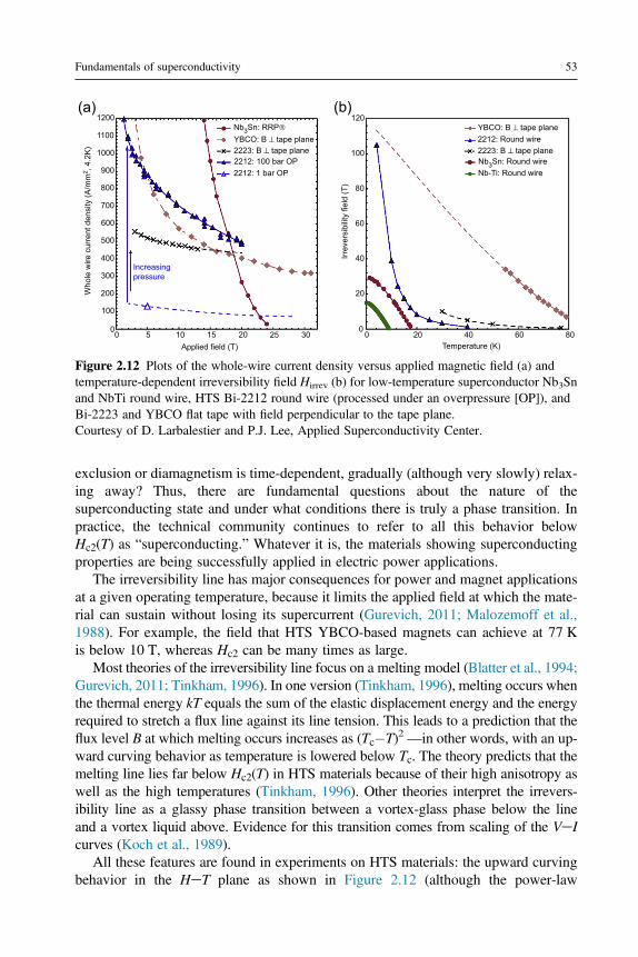
All these features are found in experiments on HTS materials: the upward curvingbehavior in the HeT plane as shown in Figure 2.12 (although the power-law

1200

1100

1000

900

800

700

600

500

400

300

200

100

00 5 10 15 20 25 30

Applied field (T)

Nb3Sn: RRP®

Nb3Sn: Round wireNb-Ti: Round wire

YBCO: B ⊥ tape planeYBCO: B ⊥ tape plane

2223: B ⊥ tape plane 2223: B ⊥ tape plane2212: 100 bar OP

2212: Round wire

2212: 1 bar OP

Increasingpressure

Who

le w

ire c

urre

nt d

ensi

ty (A

/mm

2 , 4

.2K

)

120

100

80

60

40

20

00 20 40 60 80

Temperature (K)Irr

ever

sibi

lity

field

(T)

(a) (b)

Figure 2.12 Plots of the whole-wire current density versus applied magnetic field (a) andtemperature-dependent irreversibility field Hirrev (b) for low-temperature superconductor Nb3Snand NbTi round wire, HTS Bi-2212 round wire (processed under an overpressure [OP]), andBi-2223 and YBCO flat tape with field perpendicular to the tape plane.Courtesy of D. Larbalestier and P.J. Lee, Applied Superconductivity Center.


dependence on TcT is usually found to have an exponent ofw3/2 or 4/3 rather than 2as predicted by the melting model), melting far below Hc2, the frequency dependence(Malozemoff et al., 1988), and the loss of supercurrent and critical current density witha transition to flux flow resistivity.

2.11.4.2 Flux flow resistivity

Whenever current is driven through the vortex liquid, the Lorentz force drives the fluxlines in a phenomenon called flux flow. By Lenz’s law Vwdf/dt; the moving fluxgenerates voltage and hence a flux flow resistivity. The first theory of flux flowresistivity was made by Bardeen & Stephen (1965), who assumed vortex cores of radiuswx and effective area 2px2 (Tinkham, 1996; where an extra factor of 2 has been addedto account for dissipation outside the core) were normal regions having the fullnormal-state resistivity rn. They determined the flux-flow resistivity rf from the frac-tional area occupied by these cores. Because the flux line density is just B/F0 and thearea per flux line is then F0/B, they obtained the following simple and intuitive result:

rf=rn ¼ 2px2ðF0=BÞ ¼ B=Bc2 (2.15)

using Bc2 ¼ F0/2px2. Because B is usually much smaller than Bc2 in typical experi-

ments or applications, the flux flow resistivity is small compared to rn. Nevertheless,the flux flow voltage is much larger than flux creep voltage below the irreversibilityline; therefore, sample heating can become significant. It should be noted that whileEqn (2.15) has been verified in some measurements, more often than not it comparespoorly to experiment. Many other factors play a role, such as the energy spacingsbetween the lowest quantum states inside the flux-line core; therefore, theoreticalprediction of the flux flow resistivity remains a complex topic.

One can now visualize the full VeI curve of an HTS material, which starts with thepower law behavior VwIn, rolling over to the linear flux flow resistivity behavior VwrfI, and eventually rising to the normal behavior when the current becomes so large thatthe gradient in flux causes some regions of the sample to reach B ¼ Bc2. This kind ofprogression is of great importance for the behavior of a fault current limiter (FCL), inwhich a large current drives the superconductor out of its superconducting state, firstpassing into the flux flow regime. Because the current is limited in an FCL, heatingrather than simply very high currents is what drives the sample into its normal state.

The behavior of vortex liquids is a complex topic, especially in the highly aniso-tropic HTS materials, including the concepts of Bose liquids, vortex liquid duality,disorder effects, and scaling behavior of the nonlinear resistance near the irreversibilityline. We refer the reader to the excellent review by Blatter et al. (1994) for thesefascinating topics.

2.11.5 Upper limit on Jc

There exists an upper theoretical limit on the maximum current that a superconductormay carry, even in the presence of infinite pinning force strength Fp. This maximum


upper limit is known as the “de-pairing” current density Jd. As discussed in Section 2.5,there is a corresponding decrease in entropy and hence free energy when a materialtransitions from the normal state to the superconducting state. This decrease in freeenergy is smooth at the transition temperature Tc with no latent heat evolved. Instead,this normal-to-superconducting transition is a second-order phase transition as can beseen in heat capacity measurements as a function of temperature. In contrast to thislowering of the energy by entering the superconducting state, there is the correspond-ing increase in energy (i.e., kinetic energy) of the paired electrons when they aretransporting current. Thus, the de-pairing current is the current at which the kineticenergy from the transport current exceeds that of the reduction in energy from enteringthe superconducting state and the corresponding pairing of electrons in the Cooperpair. At high-enough transport currents, it is therefore energetically favorable for thesuperconductor to transition back to the normal state. The change in energy duringscattering is maximized when the momentum change is maximized. This transition oc-curs when a carrier is scattered from one point on the Fermi surface to a diametricallyopposite one, in total reversal of direction. Jd can be shown to be equal to Hc(T)/lL.This theoretical limit of Jd can only be reached for very high Fp, with values of Jdapproaching 101213 A/m2 in HTS samples.

2.11.6 The critical surface of a type II superconductor

Now that the concepts of critical temperature Tc, upper critical magnetic field Hc2,irreversibility line Hirrev(T), and critical current density Jc0 have been discussed, allproperties can be summarized with a single concept of a critical surface of a supercon-ductor (see Figure 2.13). Shown in the figure are three axes representing temperature(y-axis), applied magnetic field (x-axis), and current density (z-axis). According to con-ventional theory for low-temperature superconductors, for values of T, H, or J that liebelow the critical surface of Hc2(T) and Jc0(T), the material remains superconducting.Above the critical surface, the material transitions from the superconducting state backto its normal resistive nonsuperconducting state.

However, we have seen that thermal activation and pinning center disorder cause adrastic modification in the critical surface for HTS materials. They give rise to an irre-versibility line in the HeT plane which lies far below Hc2(T), as shown schematicallyin Figure 2.13. Significant supercurrent can only exist below the irreversibility line, buteven here a tiny voltage can persist due to flux creep. Above the line, in the vortex-liquid region, superconductivity exists in the sense that lossless vortex currents flowaround flux lines and an energy gap persists throughout much of the sample. However,the Meissner effect and the characteristic near-zero resistivity to macroscopic currentflow are lost. The upper critical field Hc2(T) is no longer considered “critical” in thesense of a phase transition; it is a crossover. The most widely accepted picture isthat the irreversibility line is actually a glassy phase transition between a vortex-glass phase below the line and a vortex liquid above. In the vortex glass region, thecritical current is strongly suppressed by flux creep, although not enough to preventuseful applications.


Thus, for any device operating on the electric utility grid, the device must bedesigned with enough safety margin that for a given load line, the superconducting de-vice remains well below the irreversibility line to retain the characteristic superconduc-tor properties of near-zero resistance and diamagnetic screening. There are only a fewHTS electrical devices that operate with exceptions to this general rule, where thesharp change in electrical resistance experienced by the superconductor whentransitioning from the vortex liquid to vortex-liquid state is purposely used to “limit”currents in fixed voltage systems (e.g., the FCL or fault-current-limiting cables andtransformers in Chapters 5 (Section 5.6), 9, and 12).

2.12 Entropy and free energy

In Section 2.5, it can be seen that the Gibbs free energy density in the normal state isindependent of the strength of the applied field Ha. This is true because the material isessentially nonmagnetic in the normal state and acquires no magnetization in anapplied magnetic field. When a type I material enters its superconducting state(i.e., perfect diamagnetism) below Tc, the application of an applied magnetic fieldHa raises the free energy by 1/2 m0Ha

2. Thus, the difference in the Gibbs free energybetween the normal (nonmagnetic) state and the superconducting (diamagnetic) stateis given by GnGs(H) ¼ 1/2 m0(Hc

2eHa2). Using the definition for the Gibbs free

TTc

H

Hc2

Hirrev

J

Jc0

Jc0

Jc

Figure 2.13 Critical surface of a superconductor in temperature T, applied magnetic fieldH, andcurrent density J, below which supercurrent can persist. In low-temperature superconductors, thecritical surface is very close to the upper critical field Hc2 and the flux-creep-free critical currentdensity Jc0. In HTS, thermal activation and flux creep cause a reduction in the critical surface asindicated by the blue arrows, with the surface now defined by an irreversibility line Hirrev(T) anda flux-creep-reduced critical current density Jc(T). However, a superconducting gap in thedensity of electronic states and vortex currents around quantized vortex lines can persist in theentire region under Hc2. Between Hc2 and Hirrev, the flux lines are in a liquid-like state called avortex liquid; below Hirrev, in the presence of disorder in pinning center locations, the flux linesare in a disordered state called a vortex glass.


energy of G ¼ UTS þ PV m0HaM, where U is the internal energy, S is theentropy, P is the pressure, V is the volume, and M is the magnetization, and the rela-tion for entropy per unit volume S ¼ (vG/vT)p,Ha, it can be shown that the differencein entropy between the normal and superconducting states is given by the following:

Sn Ss ¼ m0Hc dHc=dT (2.16)

Because Hc(T) always decreases with increasing temperature, the quantity on theright-hand side of Eqn (2.16) must always be positive. This implies that there is alwaysan associated decrease in the entropy when going from the normal state to thesuperconducting state. Because entropy is associated with disorder, this qualitativelydemonstrates that the superconducting state is a more ordered state with lower freeenergy than the normal state (see Figure 2.14).

2.13 Bardeen, Cooper and Schrieffer (BCS) theory

There is no generally accepted microscopic explanation of high-temperature supercon-ductivity. The qualitative features of the very successful microscopic theory of low-Tcmetallic superconductors are outlined in this section.

In 1957, Bardeen, Cooper, and Schrieffer (BCS) presented the first fully quantummechanical theory to completely describe the microscopic mechanism involved insuperconductivity of LTS (Bardeen, Cooper, & Schrieffer, 1957). They were laterawarded the Nobel Prize in Physics in 1972. As outlined by Kittel (1986), the assump-tions and accomplishments of this theory were as follows:

1. The mechanism governing the elemental or intermetallic type of superconductivity is anelectronelatticeeelectron interaction mediated by the phonons (quantized lattice vibrations)in the material. This indirect interaction occurs when one electron interacts with the crystallattice and deforms it. The second electron sees this deformation and adjusts itself to takeadvantage of the redistribution of energy. Thus, the two electrons attract each other via the

Entr

opy

Temperature Tc

Tc

Fs

Fs

F N

FN

Free

ene

rgy

Temperature–1

0

Figure 2.14 Left: A qualitative plot of the difference in entropy between the (more ordered)superconducting state and the normal state. Right: Similarly, a plot of the free energy versustemperature of a superconductor and its normal state.Adapted from (Kittel, 1986, p. 326.)


lattice deformation or phonons. A common analogy used in this phonon-mediated electro-neelectron interaction is that of a bowling ball placed in the center of a soft mattress withelectrons moving around the outer periphery. Prior to the placement of the bowling ball inthe center of the mattress, the electrons at the outer bands of the Fermi surface move aroundand behave as normal metals within an electrostatically screened Coulomb potential. Oncethe bowling ball (i.e., the phonon) is placed in the center of the mattress, its presence causesan indentation which deforms the mattress (i.e., crystal lattice). The electrons traveling at theouter bands of the Fermi surface feel this lattice deformation caused by the presence of thephonon and are hence “attracted” to one another via the phonon, forming pairs, which arecalled Cooper pairs. The Cooper pairs then behave in a “cooperative” fashion.

2. The attractive interaction between electrons leads to a ground state separated from excited statesby an energy gap denoted by D. The existence of an energy gap D is the cause of many unusualelectromagnetic and optical properties in these materials. The energy gap in a classical BCS typeelectronephonon mediated superconductor is given by Eg ¼ 2D w3.5kBTc. The attractiveinteraction assumed is a generic interaction that could be produced by any pairing mechanism.This is significant because the electron pairing mechanism for the HTSs, still highlycontroversial, likely involves something other than just phonons.

3. Because the BCS ground state involves two electrons, any flux is quantized in units of 2erather than e. The magnetic flux threading the normal cores of a type II superconductor inits mixed state (see Figure 2.5) is quantized with this effective unit of charge. The flux quan-tum is defined by F0 ¼ hc/2e w2.0678 107 G cm2 or 2.0678 1015 Tm2.

2.14 Low-temperature metallic superconductors (LTS):NbTi, Nb3Sn, and MgB2

No book on HTS applications in the electric grid would be complete without at leastbriefly mentioning LTS (Scanlan, Malozemoff, & Larbalestier, 2004). Although thereis no strict guideline defining what is the cutoff temperature defining LTS and HTS,the general trend has been to call materials that appear to obey classical BCSphonon-mediated superconductivity as LTS and others, with Tc above about 30 K,as HTS. A notable exception is the well-known binary compound MgB2, which hasbeen discovered to be a superconductor with Tcw39 K in zero field (Nagamatsu,Nakagawa, Muranaka, Zenitani, & Akimitsu, 2001). MgB2, by all accounts, appearsto be the ultimate strongly coupled BCS phonon-mediated superconductor, with aTc higher than some HTS materials. Depending upon the publication, it has beenincluded in the HTS classification based upon its relatively high Tc, but more appro-priately as an LTS material based upon its electron-pairing mechanism.

Despite the tremendous progress of HTS materials since their first discovery in1986, LTS materials still dominate the commercial industrial market. By far the twomost common LTS materials widely used today are NbTi, with a Tc of w10.2 K inzero B-field, and Nb3Sn, with a Tcw18.3 K in zero B-field. They have the simple crys-tal structures shown in Figure 2.15. Examples of commercial multifilamentary wiresmade from these materials in copper matrices are shown in Figure 2.16. Even withits relatively low Tc and Hc2 w10.2 T, NbTi still remains the true workhorse of theindustry. NbTi wire’s high ductility, ease of fabrication, and relatively low cost per


unit length make it the superconductor of choice in most commercial applications, withthe largest applications being in magnetic resonance imaging and nuclear magneticresonance. NbTi is also widely used in research and high-energy physics magnets.The first and so far only commercial electric power grid application that employedNbTi was superconducting magnetic energy storage for compensation of voltagedips and sags to improve power quality, but this product has been discontinued in favorof reactive power solutions (see Chapter 1, Section 1.5.5; Malozemoff, 2012). Annualproduction of NbTi exceeds 2000 tons/year.

For applications where either higher Tc or higher magnetic fields (Hc2w22e25 T)are required, such as in fusion magnets or magnets for high-field research, Nb3Sn is thenext most widely implemented LTS conductor. There are 76 known A-15 compounds,of which 46 are known to be superconducting, with the Nb and V compounds possess-ing the highest Tc values (Smathers, 1990). The crystal structure A3B is formed by abody-centered cubic arrangement of B atoms and two A atoms centered at every face(Figure 2.15, right). Nb3Sn is a far more difficult material to work with than NbTibecause of its brittleness and sensitivity to mechanical strain. For this reason,superconducting magnets fabricated with Nb3Sn conductor are often wound prior toreaction and subsequently reacted (at >650 C) to form the superconducting Nb3Sn

Figure 2.16 Typical w0.8 mm diameter commercial multifilamentary NbTi wire (left) andNb3Sn wire (right).

Figure 2.15 Body-centered-cubic (BCC) crystal structure of the LTS material NbTi (left) andthe A-15 crystal structure for Nb3Sn, where A site is the Nb and the B site is the Sn (right).


phase. This type of wind-and-react process adds considerable cost and complexity toany superconducting system.

Nb3Sn has experienced a virtual explosion in both R&D expenditure and produc-tion capacity. Production capacities have increased more than an order of magnitudefrom w15 tons/year in 2007 to >400 tons/year (http://www.iter.org/newsline/262/1541). These advances in performance and capacity have been driven largely by theInternational Thermonuclear Experimental Reactor (ITER) fusion effort and high-energy physics accelerator magnet efforts required for luminosity upgrades at the largehadron collider located at the Euoprean Laboratory for Particle Physics (CERN: Con-seil Européen pour la Recherche Nucléaire).

Superconductivity was discovered in the binary compound magnesium di-boride orMgB2 by the Akimitsu group in 2001 (Nagamatsu et al., 2001). Interestingly, MgB2

was first synthesized back in 1953 (Jones & Marsh, 1954), but its superconductingproperties were not discovered until 2001. This “rediscovery” of MgB2 proves theadage in experimental superconductivity: “If you ever have an old material sittingon the shelf somewhere, test it for superconductivity; you never know what youmay find.”

As stated previously, despite its unusually high Tc, MgB2 appears to be the ultimatestrongly coupled LTS with a classical BCS type electronephonon mediated interac-tion. Many of the unusual electronic properties of MgB2 appear to be explained bythe presence of two different bands of electrons at the Fermi level: strongly supercon-ducting s-bonding and more weakly superconducting p-bonding, with the possibleexistence of two energy gaps (Larbalestier et al., 2001).

The commercial interest in MgB2 stems from its relatively high Tc, its high Hc2(when chemically doped; e.g., withw5% C), and its relative ease and low cost of fabri-cation. MgB2 is a binary compound whose magnetic and current-carrying properties canreadily be enhanced by chemical doping. It has a simple hexagonal crystal structure (seeFigure 2.17) and is easily synthesized (see Figure 2.18). Round multifilamentary wiresof MgB2 can be readily made from the so-called powder-in-tube (PIT) process (seeFigure 2.19), which has been successfully used in the fabrication of other round

Figure 2.17 The hexagonal crystal lattice structure of the binary compound MgB2 with latticeconstants of a ¼ 0.3086 nm and c ¼ 0.3524 nm, with a Tcw39 K in zero applied magnetic field.Adapted from Nagamatsu et al. (2001).


multifilamentary superconducting wires, such as Nb3Sn and Bi-2212 (see Figures 2.16and 2.18; Fluekiger et al., 2012). MgB2 is a candidate for superconducting electric po-wer equipment, including AC and DC power cables, motors, generators, transformers,and FCLs because of its relatively low cost of materials and fabrication, although itsinability to access the LN2 temperature range and the high refrigeration penalty forhandling AC losses at lower temperatures are significant issues for AC applicationssuch as AC cables, transformers, and FCLs.

Metal tube Precursorpowder

Multifilament drawing

Multifilament stack

Multiplecores

Powder-in-tube Single core drawing

Final heat treatment

Final multifilament wire

Figure 2.19 Schematic of the basic steps of the powder-in-tube (PIT) process used in thefabrication of round multifilamentary wire processing. Variants of the PIT process are used infabrication of round MgB2 wire, round Bi-2212 wire, and some Nb3Sn. Combined with a rollingprocess, it is also used for BSCCO-2223 tape.

Figure 2.18 A typical commercial 36 multifilament MgB2 round w1 mm diameter wire with60-mm filaments, fabricated using the powder-in-tube method.Courtesy of M. Tomisc, HyperTech, Columbus, OH.


2.15 High-temperature superconductivity

2.15.1 History

In 1986, J.G. Bednorz and K.A. Mueller discovered high-temperature superconducti-vity in LaBaCuOx (Bednorz & Mueller, 1986), for which they were quickly awardedthe Nobel Prize in physics. This material had a Tc onset of 35 K and about a 20 K widthin the resistance between Tc onset and zero. A year later, the groups of M.K. Wu andC.W. Chu (Wu et al., 1987) discovered superconductivity in the YeBaeCueO system,in which YBa2Cu3O7 (“YBCO-123”) has a Tc onset of 93 K and a transition width<5 K (higher quality present-day materials have transition widths as low as 1 K).Almost all the rare earths can be substituted for Y with similar atomic structures andhigh Tc values, and these materials are often referred to as REBCO. YBCO-REBCOwere the first materials discovered with Tc values above the liquid nitrogen boiling pointof 77 K, and they have continued to be leading materials for electric power applications.

Many more families of compounds have since been discovered, with evenhigher Tc values. Superconductivity was discovered by Maeda et al, (1988) andTallon et al. (1988) in the system BieSreCaeCueO, with Bi2Sr2Ca2Cu3O10 (“BSCCO-2223”) having the highest Tc onset of 120 K and a 10 K width (inits typical form, BSCCO-2223 has a Tc of 110 K). The TleBaeCaeCueO system,discovered by Sheng and Hermann (1988), reached an onset temperature of122e125 K with a 20 K width. To date, the Hg-Ba-Ca-Cu-O system has the highest Tcof all, reaching 135 K at ambient pressure and w160 K under high pressure (Schillinget al, 1993).

2.15.2 Crystal structure

Because this book deals primarily with HTS electrical power applications, the discus-sion is limited to the following types of superconductors. The crystal structure for theYBa2Cu3O7x compound (left-hand side) with Tcw93 K possesses both planes ofCuO2 and chains of Cu-O (see Figure 2.20, left side). X-ray analysis shows that theYBa2Cu3O7x compound has an orthorhombic unit cell with approximately seven ox-ygen atoms per formula unit. The lattice parameters of the orthorhombic cell area ¼ 3.8856 Å, b ¼ 3.815 Å, and c ¼ 11.6804 Å (see Figure 2.20).

The crystal structure for the Bi2Sr2Ca2Cu3O10 compound (right-side) with Tcw110 K has similar CuO2 planes. Note the complexity of the HTS crystal structurerelative to the LTS NbTi and Nb3Sn materials shown in Figure 2.15. HTS tapes usingthe BSCCO-2223 compound in a silver composite have been successfully fabricatedusing the PIT method with rolling into a tape shape, with especially high critical cur-rent densities achieved under high-pressure oxygen anneals (see also Figures 2.19 and2.21). These wires, produced commercially, are widely used in electric power applica-tions. A more thorough discussion is given in Chapter 3.

Early attempts at using the PIT process for YBCO-123 were quite unsuccessful dueto the strong suppression of critical current at high-angle grain boundaries. But now,tapes based on a coated-conductor geometry, with highly aligned YBCO films, have


solved the grain boundary problem and are produced commercially with excellentproperties, gaining wide use in electric power applications. A more thorough discus-sion of these wires is given in Chapter 4.

Another important wire for certain energy applications is round wire based onBi2Sr2Ca1Cu2O8 (“BSCCO-2212”) in a silver matrix (Rupich et al., 2012).BSCCO-2212 has one less CuO2 plane than BSCCO-2223 and a slightly lowerTcw85 K. The ability to make round wire with this compound is based on a specialfeature of its phase diagram, allowing formation directly from a melt phase. Althoughits Tc is comparable to that of YBCO-123, its high anisotropy leads to a much lower-lying irreversibility line, constraining its in-field applications to the 20 K range andbelow. Nevertheless, very high engineering (full wire) critical current densitieshave been achieved (Larbalestier et al., 2014), and the advantage of cabling roundwires rather than tapes makes BSCCO-2212 a strong candidate for high-field magnetcables. The round wires have diameters around 1 mm.

CuO2

CuO2

CuO2

CuO2Ca

Ca

Bi–O double layer

Bi–O double layer

Sr

Sr

Cu–O chain layer

CuO2 layer

CuO2 layer

CuO2 layer

CuO2 layer

Y

Y

Ba

Ba

Figure 2.20 Unit cell structure of Y-Ba-Cu-O-123 (left) and Bi-Sr-Ca-Cu-O-2223 (right). InYBCO, oxygen atoms sit at the vertices of the tetrahedra and squares, and Cu sits at the center ofthe base of the tetrahedral and in the middle of the squares. The CuO2 planes play a major role inthe superconductivity, while the CuO chains in YBCO act as electron donors or acceptors, whichare filled or emptied depending on the oxygen concentration of the material.

Figure 2.21 Typical multifilamentary BSCCO-2223 PIT tapes (dimension 0.3mm 4 mm).Courtesy of Sumitomo Electric Industries, Ltd.


Even though Tl and Hg-based HTS materials have even higher Tc values thanYBCO or BSCCO, they have not so far found commercial use because of theireven lower irreversibility lines (due to even higher anisotropy), difficult processing,poor stability, and the toxic nature of Tl and Hg.

2.15.3 Anisotropy

One of the key characteristics of HTS materials is the large anisotropy in their super-conducting properties. This anisotropy shows up in nearly every fundamental param-eter, including the penetration depth l and the coherence length x. Substantiallydifferent values were measured depending upon whether measurements were takenparallel to the ab crystal planes or parallel to the c-axis. This anisotropy was naturallyalso seen in the critical fields Hc1 and Hc2.

Strong anisotropy also appears in the critical current Jc, which can be an issue incertain electric power applications. Critical currents can no longer just be reportedas a function of temperature and magnetic field Jc(T,H), but also have to be reportedas a function of the applied magnetic field direction relative to the crystallographicaxes (i.e., Jc(T,H,q)). This is very different from the more isotropic LTS materials,such as NbTi and Nb3Sn, which show virtually no anisotropy in their fundamentalparameters. Shown in Figures 2.22 and 2.23 are the critical currents versus appliedmagnetic field of a REBCO-coated conductor at various temperatures, with the mag-netic field applied parallel to the ab-plane (Figure 2.22) and parallel to the c-axis(Figure 2.22). These figures show the large difference in Jc depending upon applied

7

6

5

4

3

2

1

00 2 4 6 8 10

Magnetic field (T)

H ⎜⎢ab 65 K 50 K 40 K

20 K30 K

J c (B

) / J

c (7

7 K

, 0T)

Figure 2.22 Normalized Jc versus H for applied magnetic field parallel to the ab plane of aREBCO-coated conductor tape at various temperatures. Results have been normalized to theirvalues at 77 K and self-field.Courtesy of V. Selvamanickam, University of Houston.


field direction. The behavior at intermediate angles, shown in Figure 2.24, is alsocomplex and has been the object of much study (Holesinger et al., 2008). As is oftenthe practice in HTS electrical device design, Jc(T,H) at a given temperature and appliedmagnetic field has been normalized to its Jc value at 77 K and in its own self-generatedmagnetic field (“self-field”). The full data on Jc(T,H,q) are important because different

7

6

5

4

3

2

1

0–100 –80 –60 –40 –20 0 20 40 60 80 100

Angle between magnetic field and wire normal (º)

J c(B

) / J

c(77

K, 0

T)

77 K, 3 T 65 K, 3 T

40 K, 3 T50 K, 3 T

30 K, 3 T

7.5% Zr

Figure 2.24 Normalized Jc versus angle q between a 3 T applied magnetic field and aREBCO-coated conductor tape doped with 7.5% Zr at various temperatures.Courtesy of V. Selvamanickam, University of Houston.

7

6

5

4

3

2

1

00 2 4 6 8 10

Magnetic field (T)

65 K 50 K 40 K

20 K30 K

J c(B

) / J

c(77

K, 0

T)

H ⎜⎢c

Figure 2.23 Normalized Jc versus H for applied magnetic field parallel to the c-axis of aREBCO-coated conductor tape at various temperatures. Results are normalized to the value at77 K and self-field.Courtesy of V. Selvamanickam, University of Houston.


electrical power devices require operation at different magnetic field levels andorientations, and also at different operating temperatures.

For most magnet/coil type applications in the electric power grid (e.g., transformers,energy storage, motors, generators, FCLs), it is the lowest Jc that ultimately determinesthe maximum current the device can carry because magnetic fields impinge over anentire range of angles to the ab-planes of the superconducting tape. This lower Jccaused by the anisotropy negatively affects size (footprint), mass, and cost of thedevice because the lower Jc requires more turns in a magnet for an equivalent numberof ampere-turns. One notable exception is superconducting cable, where the azimuthalmagnetic field generated by the cable during operation is both small in magnitude andalso in the most favorable direction for maximum current-carrying capacity of the HTSmaterial (see also Chapter 5, Section 5.2.1). For the Y-Ba-Cu-O tapes, this is predom-inantly in the plane of the tape.

2.16 Comparison of HTS to LTS properties and summaryof fundamental parameters

Numerous HTS materials have been discovered since the initial discovery by Bednorz& Mueller (1986). Likewise, there have been many theoretical models attempting toexplain the microscopic behavior in HTS materials and the origin of the electroneelec-tron pairing mechanism. A number of experiments have been performed, whichindicate that the high Tc superconducting mechanism may be described by a variantof the BCS theory, but just as many theories point to an entirely new electroneelectronpairing mechanism. Fortunately, the many well-developed HTS devices fabricated forthe electric power grid described in the later chapters of this book have done so withoutthe benefit or understanding of the microscopic theory of HTS. It is the phenomeno-logical theory based on the GinzburgeLandau equations, supplemented with a newunderstanding of thermal activation effects, that have been most valuable inunderstanding and optimizing HTS materials performance for grid applications.

A few key results from experiments pertaining to HTS are listed here:

• The flux quantum has been directly measured and confirmed to equal the theoretical predic-tion F0 ¼ hc/2e, which indicates electron pairing.

• Measurements of electron tunneling and electromagnetic absorption have confirmed theexistence of an energy gap D, whose magnitude at T Tc is larger than that predicted byBCS theory. However, if pseudo-gap and superconducting fluctuation effects suppressingTc are taken into account, the ratio of 2D to kTc is much closer to the BCS prediction (Tallon,Storey, & Mallett, 2012).

• The temperature dependence of the penetration depth has the same qualitative features asthose predicted by BCS theory, but the wave-function symmetry is d-wave rather than themore conventional s-wave.

• Specific heat data show a GinzburgeLandau second-order phase transition at Tc in zero field.At low temperatures, the specific heat data possess a linear term, whereas BCS theorypredicts an exponentially small electronic term.


• High-resolution X-ray data show no change in crystal structure at Tc, indicating no first-ordertransition.

In Table 2.1, we have listed some of the measured fundamental parameters forseveral industrially used superconductors. Note the large anisotropy in many ofthe fundamental parameters of HTS materials, whereas most classic LTS materialsare isotropic.

2.17 Practical superconductors

2.17.1 Priceeperformance ratio

One of the most common and effective ways to evaluate and compare the technical andeconomic viability of a superconducting wire or tape is to calculate itspriceeperformance ratio, which is typically measured in dollars per kiloamp-meteror $/kAm. This metric of comparison is also useful to electric utilities when weighingthe technical and economic benefits of superconductors versus conventional Cu- andAl-based technologies. In this simple calculation, the price per meter ($/m) of asuperconducting wire or tape is divided by its Ic performance at a specified temperature

Table 2.1 Summary of measured parameters of LTS and HTSmaterials*

Quantity NbTi Nb3Sn YBa2Cu3O7Lx Bi2Sr2Ca2Cu3Ox

Tc (K) 10 18.3 93 108e110

Hc1kc(mT, T/0) 90e110

Hc1kab(mT, T/0) 24

Hc2kc(T, T/0) 12 22e25 120

Hc2kab (T, T/0) 12 22e25 250 800

Hc (T, T/0) 0.52 1.1

xc (nm) 3e4 3.6e6 0.3e2(0.65) 0.6

xab (nm) 3e4 3.6e6 0.5e3(3.1)

lt (nm) 240 65e80 120e150

lk (nm) 240 65e80 700e800

2D(0)/kBTc 3.6e4.4 2.2e2.8

* For practical purposes, the LTS materials exhibit isotropic materials properties. As such, there is no meaning to “parallel”and “perpendicular”; values along all principal axes are the same, although some subtle differences have been discussed inthe literature (Suenaga, Ghosh, Xu, & Welsh, 1991). All parameters are taken in the limit of zero temperature.From Ginsberg (1989).


and magnetic field. Confusion can quickly arise, however, when comparing LTS toHTS materials priceeperformance ratio because of two factors: (1) the extremely largedifferences in temperature and magnetic field magnitude at which the comparisons canbe made and (2) the large anisotropy that exists in HTS materials, necessitating themagnetic field direction or angle to be specified. It is common, for example, in thehigh-energy physics accelerator magnet community, to state priceeperformance ratiosfor LTS NbTi at the operating parameters 4.2 K, 5 T; for the fusion magnet community,however, a more common reference point for LTS Nb3Sn is 4.2 K, 12 T. Because theseLTS materials are isotropic, no magnetic field direction is stated, which makes directcomparison with HTS difficult since the magnetic field direction for HTS materialsmust also be specified. The HTS community seems to have mostly settled on theconvention of reporting priceeperformance at 77 K, self-field, and then translatingthat value to the operating T, B, and q for a particular application.

In addition, these priceeperformance values can further vary even when all param-eters of T, B, and q are specified consistently due to variations in superconducting wireor tape architecture, such as amount of normal metal stabilizer present, monofilamentversus multifilament, number and size of filaments, insulated or noninsulated, etc. Theauthors have specifically refrained from specifying precise values ($/kAm) for thevarious commercial LTS and HTS wires and tapes because of the many variablesnecessary for a consistent comparison, as well as the rapidly changing costs ofHTS, which continue to decline with progress in HTS wire manufacturing and morewidespread acceptance of these HTS-based devices. But present HTS values are stillan order of magnitude or more than LTS values.

2.17.2 Why so few practical superconductors?

Since the discovery of superconductivity in 1911, thousands of materials have beendiscovered to exhibit superconductivity. There are more than 27 pure elements onthe periodic table that exhibit superconductivity under the right conditions oflow-enough temperature and high-enough pressure (Kittel, 1986). Yet, even thoughthere are so many superconductors, there are basically only eight that have any prac-tical use in electric power applications to date. These are listed in Table 2.2.

The question naturally arises: If there are so many superconductors, why are so fewused in practical superconducting applications? While the answer is complex, itbasically comes down to the fact that in order to fabricate a useful superconductingdevice, many practical engineering aspects need to be satisfied. For the device tooperate appropriately, it must have a superconducting transition temperature that iscryogenically readily accessible and not too low. Many superconducting devicesoperate in a bath of pool-boiling or subcooled liquid cryogen, such as liquid nitrogen(w65/77 K) or liquid helium (w1.2/4.2 K). Thus, the selected superconductormust have a Tc well above the boiling temperature of the cryogenic fluid to accountfor any parasitic heat loads and/or unwanted transient temperature excursions.Next, the selected superconductor must have a high-enough Jc(T,B) in the expectedbackground operating magnetic field such that the device is not too large or heavy.


In short, the energy density per unit volume or weight of the superconducting de-vice must be significantly greater than what can be obtained by a conventional non-superconducting copper or aluminum wire-based system. The method and cost offabrication of the superconducting wire must be within realistic expectations forthe contemplated device. Mechanical properties also play a significant role in thedown-selection of superconducting wires, because the wires are subject to powerfulLorentz forces when operating in large fields, and they can also experience stressesduring cool-down because of thermal contraction. Ductility is strongly preferred;however, even extremely brittle materials such as Nb3Sn, Nb3Al, and REBCOhave been successfully adapted for use in high-field superconducting devices byimbedding them in composite metallic structures and, in the case of Nb3Sn andNb3Al, winding the device before reacting to form the brittle superconducting phase.In summary, for a superconducting material to be of practical use, it must have a com-bination of properties, including Tc, Jc, Hc2 (or Hirrev), mechanical strain tolerance (ε),chemical stability, means for practical manufacturing, and a priceeperformance thatsurpass any conventional non-superconducting alternative.

2.17.3 Iron pnictides and iron chalcogenides

A new class of superconducting materials has been discovered based upon layeredFeeAs compounds (Kamihara, Watanabe, Hirano, & Hosono, 2006). These newcompounds are the so-called iron pnictides or iron chalcogenides because of their crys-tal structure. Superconducting transition temperatures as high as w55 K have beenfound in a compound of SmFeAsO (Ren et al., 2008). It remains to be seen if any ofthese new classes of materials is worth exploring for practical wire fabrication andimplementation into superconducting devices for the electric power grid. In addition

Table 2.2 Superconductors used in practical power devices

Superconductor Transition temperature (K)

Nb 9.5

NbTi 9.5

Nb3Sn 18.3

Nb3Al 18.8

MgB2 39

REBa2Cu3O7 93

Bi2Sr2Ca1Cu2O8 85

Bi2Sr2Ca2Cu3O10 108e110

Nb has primarily been used in high-Q cavities, while all the others have been used in wire form for a variety of magnets,coils, and cables. The listed transition temperature is in zero-applied field.


to having adequate Tc, Jc, Hc2 (and Hirrev), anisotropy in Jc and Hc2, mechanicalproperties, and priceeperformance for a given application, their performance in at leastone area must exceed that of the existing superconducting materials listed in Table 2.2in order to justify the significant time and fiscal expenditure required to turn them intopractical useful wire architectures; that advantage has not yet been identified.

Acknowledgment

The authors wish to thank Ben Andrews for his help in the production of figures for this chapter.

References

Abrikosov, A. A. (1957). On the magnetic properties of superconductors of the second group.Zh Eksperim.i Teor Fiz, 32, 1442 [Soviet Physics. JETP, 1957, 5, 1174].

Anderson, P. W., & Kim, Y. B. (1964). Hard superconductivity: theory of the motion ofAbrikosov flux lines. Reviews of Modern Physics, 36, 39e43.

Bardeen, J., Cooper, L. N., & Schrieffer, J. R. (1957). Theory of superconductivity. PhysicalReview, 108, 1175e1204.

Bardeen, J., & Stephen, M. J. (1965). Theory of the motion of vortices in superconductors.Physical Review, 140, 1197.

Bean, C. P. (1962). Magnetization of hard superconductors. Physical Review Letters, 8,250e253.

Bean, C. P. (1964). Magnetization of high-field superconductors. Reviews of Modern Physics,36, 31e39.

Bednorz, J. G., & Mueller, K. A. (1986). Possible high Tc superconductivity in the Ba-La-Cu-Osystem. Zeitschrift f€ur Physik B, 64, 189e193.

Blatter, G., Feigel’man, M. V., Geshkenbein, V. B., Larkin, A. I., & Vinokur, V. M. (1994).Vortex matter. Reviews of Modern Physics, 66, 1125e1388.

Campbell, A. M., & Evetts, J. E. (1972). Flux vortices and transport currents in type II super-conductors. Advances in Physics, 21, 199e428.

Civale, L. (1997). Vortex pinning and creep in high temperature superconductors with columnardefects. Superconductor Science and Technology, 10, A11.

Civale, L., Krusin-Elbaum, L., Thompson, J., Wheeler, R., Marwick, A. D., Kirk, M. A., et al.(1994). Reducing vortex motion in YBaCuO crystals with splay in columnar defects.Physical Review B, 50, 4102.

Civale, L., Marwick, A. D., McElfresh, M. W., Worthington, T. K., Malozemoff, A. P.,Holtzberg, F. H., et al. (1990). Defect independence of the irreversibility line in proton-irradiated Y-Ba-Cu-O crystals. Physical Review Letters, 65, 1164e1167.

De Bruyn Ouboter, R., Van Delft, D., & Kes, P. H. (2012). Discovery and Early History ofSuperconductivity. In H. Rogalla, & P. H. Kes (Eds.), 100 years of superconductivity (pp.1e29). Boca Raton, FL: CRC Press.

Feigel’man, M. V., Geshkenbein, V. B., Larkin, A. I., & Vinokur, V. M. (1989). Theory ofcollective flux creep. Physical Review Letters, 63, 2303e2306.

Fisher, M. P. A. (1989). Vortex glass superconductivity: a possible new phase in bulk high Tcoxides. Physical Review Letters, 62, 1415e1418.


Fluekiger, R., & Kumakura, H. (2012). The MgB2 story. In H. Rogalla, & P. H. Kes (Eds.),100 years of superconductivity (pp. 702e712). Boca Raton, FL: CRC Press.

Fulde, P., & Ferrell, R. A. (1964). Superconductivity in a strong spin-exchange field. PhysicalReview, 135, A550.

Fruchter, L., Malozemoff, A. P., Campbell, I. A., Sanchez, J., Konczykowski, M., Griessen, R.,et al. (1991). Low temperature magnetic relaxation in YBaCuO e evidence for quantumtunneling of vortices? Physical Review B, 43, 8709.

Ginsberg, D. M. (1989). Physical properties of high temperature superconductors I. NewJersey: World Scientific, 46e48.

Ginzburg, V. L., & Landau, L. D. (1950). On the theory of superconductivity. Zh Eksperim TeorFiz, 20, 1064.

Gurevich, A. (2011). To use or not to use cool superconductors. Nature Materials, 10, 255e259.Hao, Z., Clem, J. R., McElfresh, M. W., Civale, L., Malozemoff, A. P., & Holtzberg, F. (1991).

Model for the reversible magnetization of high-k type II superconductors: application tohigh-Tc superconductors. Physical Review B, 43, 2844e2852.

Holesinger, T., Civale, L., Maiorov, B., Feldmann, M., Coulter, Y., Miller, D., et al. (2008).Progress in nano-engineered microstructures for tunable high current high-temperaturesuperconducting wires. Advanced Materials, 20, 391e407.

Jones, M. E., &Marsh, R. E. (1954). The preparation and structure of magnesium boride, MgB2.Journal of the American Chemical Society, 76(5), 1434.

Kamerlingh Onnes, H. (1911e1912). On the sudden change in the rate at which the resistance ofmercury disappears. Communications from the Physical Laboratory of the University ofLeiden, 124c (Nov. 1911); English translation in KNAW Proceedings, 14II. Amsterdam1912, pp. 818e821.

Kamihara, Y., Watanabe, T., Hirano, M., & Hosono, H. (2006). Iron-based layered supercon-ductor LaOFeP. Journal of the American Chemical Society, 128(31), 10012e10013.

Kittel, C. (1986). Introduction to solid state physics (6th ed.). New York: John Wiley & Sons.Koch, R. H., Foglietti, V., Gallagher, W. J., Koren, G., Gupta, A., & Fisher, M. P. A. (1989).

Experimental evidence for vortex-glass superconductivity in Y-Ba-Cu-O. Physical ReviewLetters, 63, 1511.

Larbalestier, D. C., Cooley, L. D., Rikel, M. O., Jiang, J., Patnaik, S., Cai, X. Y., et al. (2001).Strongly linked current flow in polycrystalline forms of the superconductor MgB2. Nature,410(6825), 186e189.

Larbalestier, D., Jiang, J., Trociewitz, U., Kametani, F., Scheuerlein, C., Dalban-Canassy, M.,Matras, M., Chen, P., et al. (2014). Isotropic round-wire multi-filament cuprate super-conductor for generation of magnetic fields above 30 T. Nature Materials, 13, 375e381.

Larkin, A. I., & Ovchinnikov, Yu. N. (1964). Nonuniform state of superconductors. Zh EkspTeor Fiz, 47, 1136.

London, F., & London, H. (1935). The electromagnetic equations of the supraconductor.Proceedings of the Royal Society of London, A149, 71.

Maeda, H., Tanaka, Y., Fukutomi, M., & Asano, T. (1988). A new high-Tc oxide supercon-ductor without a rare earth element. Japanese Journal of Applied Physics, 27, L209.

Maiorov, B., Baily, S. A., Zhou, H., Ugurlu, O., Kennison, J. A., Dowden, P. C., et al. (2009).Synergetic combination of different types of defects to optimize pinning landscape usingBaZrO3-doped YBa2Cu3O7. Nature Materials, 8, 398.

Malozemoff, A. P. (1991). Flux creep in high temperature superconductors. Physica C, 185-9,264e269.

Malozemoff, A. P. (2012). Second-generation high-temperature superconductor wires for theelectric power grid. Annual Review of Materials Research, 42, 373e397.


Malozemoff, A. P., Carter, W. L., Gannon, J., Joshi, C. H., Miles, P., Minot, M., et al. (1992).Progress in the development of bismuth-based high-temperature superconducting tapes.Cryogenics, 32, 478e484.

Malozemoff, A. P., & Fisher, M. P. A. (1990). Universality in the current decay and flux creep ofYBaCuO high temperature superconductors. Physical Review B, 42, 6784.

Malozemoff, A. P., Worthington, T. K., Yeshurun, Y., Holtzberg, F., & Kes, P. H. (1988).Frequency dependence of the ac susceptibility in a Y-Ba-CuO crystal: a reinterpretation ofHc2. Physical Review B, 38, 7203e7206.

Malozemoff, A. P., & Yamada, Y. (2012). Coated conductor: second generation HTS wire. InH. Rogalla, & P. Kes (Eds.), 100 years of superconductivity (pp. 689e702). Boca Raton,FL: CRC Press, Taylor & Francis Group.

Meissner, W., & Ochensenfield, R. (1933). Ein neuer Effeckt bei Eintritt der Supraleitfaehigkeit.Naturwissenschaften, 21, 787.

Nagamatsu, J., Nakagawa, N., Muranaka, T., Zenitani, Y., & Akimitsu, J. (2001). Supercon-ductivity at 39 K in magnesium diboride. Nature, 410, 63e6424.

Norris, W. T. (1970). Calculation of hysteresis losses in hard superconductors carrying ac:isolated conductors and edges of thin sheets. Journal of Physics D, 3, 489.

Pippard, A. B. (1953). An experimental and theoretical study of the relation between magneticfield and current in a superconductor. Proceedings of the Royal Society of London, 216,1127.

Ren, Z.-A., Che, G.-C., Dong, X.-L., Yang, J., Lu, W., Yi, W., et al. (2008). Superconductivityand phase diagram in iron-based arsenic-oxides ReFeAsO1-d (Re ¼ rare-earth metal)without fluorine doping. Europhysics Letters, 83, 17002.

Rose-Innes, A. C., & Rhoderick, E. H. (1978). Introduction to superconductivity (Vol. 6). NewYork: Pergamon Press.

Rupich, M. W., & Hellstrom, E. E. (2012). Bi-Ca-Sr-Cu-O wire. In H. Rogalla, & P. H. Kes(Eds.), 100 years of superconductivity (pp. 671e689). Boca Raton, FL: CRC Press.

Scanlan, R. M., Malozemoff, A. P., & Larbalestier, D. C. (2004). Superconducting materials forlarge scale applications. Proceedings of the IEEE, 92, 1639e1654.

Schilling, A., Cantoni, M., Guo, J. D., & Ott, H. R. (1993). Superconductivity above 130 K inthe Hg-Ba-Ca-Cu-O system. Nature, 363, 56e58.

Sheng, Z. Z., & Hermann, A. M. (1988). Bulk superconductivity at 120 K in the Tl-Ca/Ba-Cu-Osystem. Nature, 332, 138.

See http://www.iter.org/newsline/262/1541.Silsbee, F. B. (1916). A note on electrical conduction in metals at low temperatures. Journal of

the Washington Academy of Sciences, 6, 597.Smathers, D. B. (1990). A15 superconductors. In American society for metals: vol. 2. Metals

Handbook (10th ed.) (pp. 1060e1076).Suenaga, M., Ghosh, A. K., Xu, Y., & Welsh, D. O. (1991). Irreversibility temperatures of

Nb3Sn and NbTi. Physical Review Letters, 66, 1777.Tallon, J. L., Buckley, R. G., Gilberd, P. W., Presland, M. R., & Brown, I.W.M. (1988). High-

Tc superconducting phases in the series Bi2.1(Ca,Sr)nþ1CunO2nþ4þd. Nature, 333,153e156.

Tallon, J. L., Storey, J. G., & Mallett, B. (2012). The design of high-Tc superconductors e roomtemperature superconductivity? Physica C, 482, 45e49.

Thompson, J. R., Sun, Y. R., Civale, L., Malozemoff, A. P., McElfresh, M. W., Marwick, A. D.,et al. (1993). Effect of flux creep on the temperature dependence of the current density inYBaCuO crystals. Physical Review B, 47, 14440e14447.


http://www.iter.org/newsline/262/1541

Tinkham, M. (1996). Introduction to superconductivity (2nd ed.). New York: McGraw-Hill,Inc., 336e337.

Warnes, W. H., & Larbalestier, D. C. (1986). Critical current distributions in superconductingcomposites. Cryogenics, 26, 643e653.

Weber, H. W. (2011). Radiation effects on superconducting fusion magnet components.International Journal of Modern Physics E, 20, 1325e1378.

Wu, M. K., Ashburn, J. R., Torng, C. J., Hor, P. H., Meng, R. L., Gao, L., et al. (1987). Su-perconductivity at 93 K in a new mixed phase Y-Ba-Cu-O compound system at ambientpressure. Physical Review Letters, 58(9), 908e910.

Yeshurun, Y., Malozemoff, A. P., & Shaulov, A. (1996). Magnetic relaxation in high temper-ature superconductors. Reviews of Modern Physics, 68, 911e950.


Date post:	25-May-2018
Category:	Documents
Upload:	vuonglien
View:	217 times
Download:	0 times

2 - Fundamentals of superconductivity - SciTech...

Documents