130
© 2006 Amir Hosein Kamalizad All Rights Reserved

© 2006 Amir Hosein Kamalizad All Rights Reserved

ii
The dissertation of Amir Hosein Kamalizad
is approved and is acceptable in quality
and form for publication on microfilm:
________________________________________
________________________________________
________________________________________
________________________________________ Committee Chair
University of California, Irvine
2006

iii
Dedication
To my family,
for their true love and support.
iv
Table of Contents LIST OF FIGURES...............................................................................................................vi
LIST OF TABLES...............................................................................................................vii
Acknowledgements .......................................................................................................viii
CURRICULUM VITAE.........................................................................................................ix
Abstract of the Dissertation ...........................................................................................xiii
Chapter 1 Introduction ..................................................................................................1 1.1 Overview ..........................................................................................................1 1.2 Background and Related Works.......................................................................2 1.3 MaRS Motivation .............................................................................................5
Chapter 2 MaRS Architecture.......................................................................................9 2.1 Top-level Architecture View............................................................................9 2.2 Architecture Details........................................................................................12
2.2.1 Routers and Channels .............................................................................16 2.2.2 FPU.........................................................................................................19
2.3 The Second Layer of Inter-PE Connections...................................................20 2.4 Accelerator for Viterbi Decoding...................................................................22 2.5 Instruction Set Architecture............................................................................23 2.6 MaRS RTL Implementation ...........................................................................23
Chapter 3 MaRS Programming Model & Applications..............................................24 3.1 Parallel Programming on MaRS.....................................................................24 3.2 Example: 16-Point Complex FFT ..................................................................25
3.2.1 FFT Algorithm........................................................................................26 3.2.2 Mapping FFT..........................................................................................29
3.3 EEMBC Telecomm Suite ...............................................................................32 3.3.1 Autocorrelation.......................................................................................34 3.3.2 DSL bit allocation...................................................................................35 3.3.3 Convolutional encoder............................................................................36 3.3.4 FFT .........................................................................................................37 3.3.5 Viterbi decoder .......................................................................................39 3.3.6 EEMBC Telecomm suite results ............................................................40
Chapter 4 IEEE 802.11a PHY Algorithms .................................................................41 4.1 IEEE 802.11a system overview and background ...........................................41 4.2 Channel Model and Simulation Parameters ...................................................44 4.3 Receiver Algorithms.......................................................................................46
4.3.1 Frame detection, coarse timing and coarse CFO acquisition .................47 4.3.2 Fine Timing Synchronization, Fine CFO and Channel Estimation........50
v
4.3.3 Tracking Algorithms ..............................................................................57 4.3.4 Outer receiver .........................................................................................59
4.4 Tasks partitioning and mapping .....................................................................67 4.4.1 Mapping the Viterbi Algorithm..............................................................70 4.4.2 Mapping FFT on MaRS..........................................................................81
Chapter 5 Reed Solomon Decoder..............................................................................84 5.1 Syndromes Computation ................................................................................87 5.2 Berlekamp Massey Algorithm........................................................................89 5.3 Roots search (Chien search) algorithm...........................................................90 5.4 Forney Algorithm ...........................................................................................91 5.5 Comparisons and Conclusion .........................................................................92
Chapter 6 Implementation of Parameterized Viterbi Decoder in MaRS ....................94 6.1 Convolutional Codes ......................................................................................95
6.1.1 Data Communication Pattern ...............................................................101 6.2 Convolutional Turbo Code ...........................................................................101
6.2.1 CTC Encoding ......................................................................................102 6.2.2 Turbo Decoder......................................................................................103
Chapter 7 Conclusions ..............................................................................................107 7.1 Contributions ................................................................................................107 7.2 Future Direction of MaRS............................................................................108
Bibliography .................................................................................................................112
Appendix A ..................................................................................................................116

vi
L IST OF FIGURES Figure 1-1– MorphoSys Architecture............................................................................ 7 Figure 1-2– SAHARA Architecture.............................................................................. 8 Figure 2-1– (Left) Inter-PE connection in homogeneous MaRS with a 4-stage macro-
pipeline, (Right) an application specific PE been plugged in array .................... 10 Figure 2-2– Macro-pipeline model on MaRS ............................................................. 11 Figure 2-3– PEs 2-D mesh network ............................................................................ 12 Figure 2-4–Architecture of MaRS PE’s execution unit.............................................. 13 Figure 2-5–A multicast to a 4-rectangle macro-block................................................. 15 Figure 2-6–Second layer of interconnection network in MaRS.................................. 21 Figure 3-1 – Synchronous data flow programming model.......................................... 25 Figure 3-2 – FFT Algorithm illustration ..................................................................... 28 Figure 3-3 – 2-point DFT butterfly ............................................................................. 29 Figure 3-4 – Simplified 2-point DFT butterfly............................................................ 29 Figure 3-5 – Layout of PEs in the array ...................................................................... 30 Figure 3-6 – 16-point complex FFT algorithm mapping on MaRS ............................ 31 Figure 4-1 – IEEE 802.11a Transmitter ...................................................................... 43 Figure 4-2 – Format of IEEE 802.11a frame............................................................... 44 Figure 4-3 – IEEE 802.11a Receiver........................................................................... 47 Figure 4-4 – Short Training Sequence normalized correlation Metric........................ 49 Figure 4-5 – Long training sequence metric................................................................ 53 Figure 4-6 – Histograms showing fine timing synchronization performance............. 54 Figure 4-7 – Residual CFO; illustrates acquisition algorithm performance................ 56 Figure 4-8 – Channel estimation performance in SNR=20dB .................................... 57 Figure 4-9 – Post tracking plots with residual CFO of 2.48 KHz:
Received constellation real and imaginary amplitude vs. time ........................... 58 Figure 4-10 – Hard-decision de-mapping for 64 QAM............................................... 60 Figure 4-11a-f – Partitions of constellation to subsets ‘0’ and ‘1’ for 64QAM.......... 64 Figure 4-12 – Diagram of the receiver algorithm........................................................ 68 Figure 4-13 – Tasks allocation on PEs ........................................................................ 69 Figure 4-14 – Fully node parallel architecture ............................................................ 72 Figure 4-15 – Communication pattern needed in state metric update......................... 75 Figure 5-1 – Reed Solomon encoder architecture ....................................................... 86 Figure 5-2 – Tasks allocation on PEs.......................................................................... 93 Figure 6-1 – Trellis diagram for a convolutional code................................................ 96 Figure 6-2 – Trellis traversal for convolutional code with rate k/n............................. 99 Figure 6-3 – Block diagram of turbo decoder ...........................................................104 Figure 6-4 – Prologue state for decoding circular convolutional turbo code ............ 105
vii
L IST OF TABLES Table 3-1 – Execution statistics on RTL code using cadence simulator and sim-vision
............................................................................................................................. 32 Table 4-1 – SNR gain corresponding to 8% PER for different rates .......................... 67 Table 4-2 –Mapping results for IEEE 802.11a receiver kernels ................................. 70 Table 4-3 –Allocation of trellis states in each PE ....................................................... 76 Table 4-4 –Instructions in the first cycle..................................................................... 77 Table 4-5 –State metrics distribution after first cycle ................................................. 77 Table 4-6 – Instructions in the second cycle ............................................................... 78 Table 4-7 –State metrics distribution after second cycle............................................. 78 Table 4-8 – Instructions in the third cycle................................................................... 79 Table 4-9 –State metrics distribution after third cycle ................................................ 79 Table 4-10 –Instructions in the fourth cycle................................................................ 80 Table 4-11 –State metrics distribution after fourth cycle............................................ 80 Table 5-1 –Comparison of number of cycles for Reed Solomon decoding software
implementation on different architectures........................................................... 93 Table 6-1 –Computation breakdown for decoding of 1-bit using Viterbi decoder ... 100 Table 6-2- Instructions break-down for decoding one bit using Viterbi algorithm .. 100

viii
Acknowledgements
First and foremost I would like to thanks my advisor, Professor Nader
Bagherzadeh, for giving me the opportunity to work in his group. His help, support
and guidance have been outstanding. Also I would like to thank my dissertation
committee members, Professor Ayanoglu and Professor Gaudiot. This work would be
impossible without their work. I would also like to thanks professors Givargis and
Doemer for serving on my qualification exam committee and Professor Tabrizi for his
major contribution to the MaRS project.
I would also like to thank my group members in the Advanced Computer
Architecture Lab, Haitao Du, Chengzhi Pan, Bita Gorji-Ara, Jun Bahn, and Akira
Hatanaka. The group discussions and conversations have led to many of the ideas
implemented in the project. I would also like to thank my friends in UCI EECS
department specially Ahmad, Mahyar and Amir, who made UCI like a home for me.
Special thanks will go to DARPA, AFRL, NSF, Broadcom, State of California
and UCI EECS department who have been supported me throughout my graduate
studies. Their generous grants have sponsored this research.
Last, but certainly not least, I would like to thank my family. They have
always been true lovers and supporters of mine. I really appreciate my parents,
brother and sisters for their true love and friendship and providing me the atmosphere
to pursue my dream of graduate studies. Also I should really thank my uncle and his
wife who are my only relatives in US. Their helps, hints, caring and supports have
been outstanding.

ix
CURRICULUM VITAE Amir Hosein Kamalizad 2211 Verano Place, Irvine, CA 92617 Telephone (Work) 949.824.2481 (Cell) 949.400.9893 [email protected] Education
University of California at Irvine (Henry Samueli School of Engineering), Ph.D. Electrical and Computer Engineering (Anticipated graduation Winter 2006) University of California at Irvine (Henry Samueli School of Engineering), Master of Science in Electrical and Computer Engineering, March 2002 Sharif University of Technology, Tehran, Iran, Bachelor of Science in Electrical Engineering concentrating in electronics, June 2000 Experience
Morpho Technologies Irvine, California (June 2005 – Present) June 2005 – Present Engineering intern, systems and firmware group, WiMAX/WiBRO project, Irvine, CA Engineering intern working with system engineers to develop a WiMAX/WiBRO transmitter and receiver based on OFDMA physical layer and helping the firmware engineers to map the kernels on the reconfigurable architecture. Duties include: In depth studying of IEEE 802.16e and WiBRO and preparing explanatory
documents for the project Developing the Matlab floating-point and fixed-point model for the OFDMA
physical layer transmitter and receiver Developing architecture friendly algorithms to facilitate easier mapping of the
algorithms on MorphoSys architecture Feasibility study on DVB_H Advanced Computer Architecture Lab EECS Department, UC Irvine, Irvine, California (January 2001 – Present) April 2002 – Present Graduate Student Researcher, MaRS Project, Irvine, CA

x
Ph.D. student working as a lead student on a Macro-pipeline Reconfigurable System designed for wireless and multimedia application particularly OFDM applications. Duties include: Preliminary studies on WPAN using Multi-band OFDM UWB technology,
WiMAX and DVB-H Parallel mapping of a Reed-Solomon decoder on MaRS architecture for DVB and
WiMAX applications Parallel mapping of a FFT parameterized library for a wide range of applications
on MaRS Parallel mapping of a fast fully programmable Viterbi decoder with different
constraint lengths on MaRS Mapping EEMBC telecomm. suit on MaRS architecture to evaluate its
performance Mapping a fully programmable IEEE 802.11a WLAN receiver on MaRS Developing a complete system simulator for IEEE 802.11a system including
synchronization algorithms and a soft decision BICM Viterbi decoder Mentoring undergrad and new graduate students Generating test-benches to test the RTL code Designing an application specific processing element for IEEE 802.11a Viterbi
decoder using VHDL RTL coding and cadence design flow Contributing to the ISA, interconnection network, hardware accelerators,
application specific units and basically design of MaRS January 2001 – March 2002 Graduate Student Researcher, MorphoSys, Irvine, CA Working with a team of graduate students and researchers on the second generation of MorphoSys, a 2D-array SIMD-type architecture, and mapping some of the kernels on the architecture. Duties undertaken included: Working on a modified version of MorphoSys with special interconnect and PE
architecture optimized for Viterbi decoder Developing hand optimized assembly code for FFT, frequency offset tracking and
fine timing synchronization executable on MorphoSys simulator Developing a Matlab code including a detailed fixed point code for 8k-point
complex FFT Developing test-bench and debugging the cycle accurate simulator for MorphoSys Interacting with design engineers and introducing new instructions, features and
hardware accelerators to architecture Integrated Systems Lab EE Department, Sharif University of Technology, Tehran, Iran (June 2000 – January 2001) June 2000 – January 2001

xi
Computer Networks Computer Architecture Design and Analysis of Algorithms Advanced System Software VLSI Microarchitecture Numerical processors
Error Control Coding Advanced Digital Communication Wireless Communication SoC modeling and description (Spec-C, System-C) DSP processors ASIC low power design methodology Implementation of wireless communication
systems
DSP
Researcher, Tehran, Iran Researcher working with a graduate student simulating different techniques to reduce the PAPR of OFDM signal. Duties include: Coding the PAPR reduction algorithms in Matlab with the GUI Literature survey on existing algorithm, their advantages and disadvantages and
implementation overhead Studying the IEEE 802.11a WLAN standard and developing a simple transmitter-
channel-receiver package with the GUI using Matlab as my senior design project Awards and Honors
UCI EECS department PhD dissertation fellowship (Spring 2006) UCI CPCC prestigious fellowship awarded (2003) Accepted for graduate studies in Iran through entrance exam Ranked 122 out of 300000 participants in Iranian nationwide entrance exam for
undergraduate studies IEEE student member since 1999 Served as a reviewer for IEEE transactions on computers, IEEE VTC, Euro-Par,
DATE, IEEE SBAC-PAD, ACM computing frontiers, ITCC and etc. Designed the webpage for ITCC 2004/ITNG 2006 special track on reconfigurable
DSP Professional Development Successfully completed the following graduate level courses at UC Irvine: Successfully completed the following graduate level course at Sharif University of Technology:
Demonstrated organization and communication skills serving as a teaching assistant at UC Irvine:
xii
EECS 31 LA, Teaching Assistant, Introduction to digital systems Lab. Fall 2004 EECS 31 LB, Head Teaching Assistant, advanced digital systems Lab. Winter
2004
Developed and demonstrated following skills doing course projects and research: In-depth knowledge of OFDM and coding algorithms Knowledge of WCDMA and 3G Doppler mitigation techniques in OFDM Belief propagation for decoding LDPC codes Block turbo code simulation using MATLAB Turbo code and duo-binary turbo code knowledge Beam-forming using LMS algorithm Design of a microprocessor from RTL to GDSII and applying low power
methodology to it Custom cell design all the way to layout using MAGIC Windows, UNIX, MAC/OS Experience with C/C++, Spec C Familiar with Simulink, HSPICE, IRSIM, ORCAD Publications H. Parizi, A. Niktash, A. Kamalizad, N. Bagherzadeh, “A Reconfigurable Architecture for Wireless Communication Systems,” To appear in ITNG 2006 A. Kamalizad, N. Tabrizi, N. Bagherzadeh, “MaRS: A Programmable DSP architecture for wireless communication systems,” to appear in IEEE ASAP 2005. A. Kamalizad, R. Plettner, C. Pan, N. Bagherzadeh, “Fast Parallel Soft Viterbi Decoder Mapping on a Reconfigurable DSP Platform,” IEEE SoC conference, 2004. A. Kamalizad, N. Bagherzadeh, “Synchronization Algorithms for IEEE 802.11a Receiver,” accepted for publication in IEEE VTC Fall 2004. A. Kamalizad, N. Bagherzadeh, “Performance of soft decoding using channel state information in IEEE 802.11a,” accepted for publication in VTC spring 2004. N. Tabrizi, N. Bagherzadeh, A. Kamalizad, H. Du, “MaRS: A Macro-pipelined Reconfigurable System,” In proceedings of ACM conference on computing frontiers A. Kamalizad, C. Pan, N. Bagherzadeh, “Fast parallel FFT on a reconfigurable computation platform,” In Proceedings of 15th Symposium on Computer Architecture and High Performance Computing, SBAC-PAD 2003. C. Pan, N. Bagherzadeh, A. Kamalizad, A. Koohi, "Design and analysis of a programmable single-chip architecture for DVB-T base-band receiver," in Proceedings of Design, Automation and Test in Europe (DATE03). Patents A. Kamalizad, A. Niktash, “Adaptive FFT scaling in OFDMA systems,” submitted
xiii
Abstract of the Dissertation
A Multiprocessor Array Architecture for DSP and Wireless Applications and Case Study of an IEEE 802.11a Receiver Implementation
By
Amir Hosein Kamalizad
Doctor of Philosophy in Electrical and Computer Engineering
University of California, Irvine, 2006 Professor Nader Bagherzadeh, Chair
Multimedia processing and wireless communication are increasingly gaining
attention in both academia and industry aiming at the design of low-power, high-
performance, and flexible solutions to efficiently handle complex tasks in real-time
and in a cost-effective manner. Currently, with different standards delivering
different services for instance WLAN [1], WPAN [2], WMAN [3], CDMA based
cellular networks and their high speed extensions [4], DVB-H [5-7] the importance of
programmability is highlighted as convergence of devices is the industry trend.
In this research, we investigate two-dimensional multiprocessor array
architectures targeting Multimedia and wireless applications. Having the experience
of the MorphoSys project [8-12] and being aware of its shortcomings and strengths,
we propose MaRS, a Macro-pipeline Reconfigurable System [13-14]. As an example
of a high-rate complicated application, we used the physical layer of IEEE 802.11a
[15] Wireless LAN standard throughout the design process as an example of
application-platform co-design. As a part of this research, a fully compliant IEEE
802.11a simulator is implemented using Matlab leading to a set of VLSI suitable
xiv
synchronization algorithms [16] and a novel soft decision Viterbi decoder
incorporating channel state information [17].
In order to further evaluate the performance of MaRS, the communication suit
of EEMBC benchmarks [18] are investigated along with some future applications. It
is noticed that forward error correction coding, is the killer application; therefore,
popular FEC coding algorithms including different types of convolutional codes, and
Reed Solomon codes are studied in details and the proposed modification to
architecture and ISA are proposed along with the analytic evaluation of their
computation cost.
The organization of the dissertation is as follows. In the introduction, the
previous work, background and motivation for this work are presented. Then the
MaRS architecture is elaborated in details. Chapter three explains the programming
model of MaRS with some examples of parallel mapping on the architecture and
presents some parallel application benchmark comparison. An overview of the IEEE
802.11a model and proposed algorithms are presented in next Chapter along with the
algorithms mapping in a pipeline fashion on a 10x10 array of processing elements in
MaRS. Chapter 5 treats the mapping of Reed Solomon decoder on MaRS array.
Chapter 6 is dedicated to the study of parameterizable Viterbi decoder on MaRS.
Future works and conclusions are presented in the final Chapter.

1
Chapter 1 Introduction
Introduction 1.1 Overview
In the past decades, the scaling of the VLSI technology according to Moore’s
law [19], has given processor architects a large amount of real estate to maneuver.
Increasing the number of functional units and processing elements besides increasing
the size of on-chip memory has been pushing the performance of processors to the
limit. Optimum resource utilization, i.e. using the available silicon, seems to be the
next challenge. Meanwhile, application domain has been constantly demanding more
performance. Wireless communication is an area with enormous market potential and
ever increasing algorithms complexity and throughput. In the last several years,
wireless industry has evolved from basic pagers to delivering broadband internet and
DVD quality video.
Programmability is going to be the key to success in wireless and DSP market.
A multimode radio capable of addressing diverse media and protocols requirement
will be the ultimate solution where, the hardware can reconfigure itself to implement
the new application. Reconfiguration is done in instruction level in each processing
element and the way that Processing Elements (PE) are connected to each other.
2
Reconfigurable processors are intermediate solutions for digital applications.
While they almost offer the versatility of General-purpose processors, they approach
the performance of fixed Application-Specific Integrated Circuits (ASICs). They
facilitate using a once designed and tested hardware for different applications.
Wireless communication and signal processing applications, on the other
hand, utilize a few kernels that consume a large fraction of the total execution time
and energy. For these applications a considerable performance boost and power
savings may be achieved by executing the dominant kernels on optimized processing
elements, resulting in a domain specific processor which is a trade-off between
flexibility and performance.
With MorphoSys and some other reconfigurable projects such as PACT XPP
[20], RAW [21], IPFlex [22] and etc. being introduced, reconfigurable DSPs are
expected to dominate the market and be the choice of future mobile systems or set top
box modems where several standards should be supported.
1.2 Background and Related Works
The existing DSP and multimedia processors cover a wide range in terms of
both architecture and functionality. Customized DSP processors generally use VLIW
with issue width of as high as 8 with powerful memory and register file access and
hardware accelerators for performance hungry applications. High performance
general purpose processors on the other hand, have been using superscalar
architecture. SIMD extension and vector processing with sub-word parallelism have
also been used to boost the performance.
3
TI high performance C64x [23] uses VelociTI [24] architecture which is
VLIW with issue-width of 8 to utilize the parallelism inherent in DSP applications. It
also uses a deep pipelined datapath which enables TI to achieve clock rates as high as
1 GHz. In addition to a high clock rate, C64x DSPs can do more work each cycle
with built-in instruction extensions for targeted applications. These extensions include
new instructions to accelerate performance in key application areas such as digital
communications infrastructure and video and image processing. A good example is
the embedded Galois Field (GF) Multiply-Accumulate (MAC) unit used in Reed-
Solomon encoding and decoding.
Starcore is a joint venture of three semiconductor giants namely Freescale
(formerly Motorola), Infineon and Agere. Starcore SC140 [25] is adopted by many
System-on-Chip makers as the DSP core. It can execute up to 6 instructions
concurrently using its VLIW decoder. It supports different access width move
instructions with powerful address generator units and special instructions for Viterbi
decoding.
Sun UltralSPARC [26] is a superscalar processor with an issue rate of up to 4,
featuring the Visual Instruction Set (VIS) multimedia extension, to accelerate data-
parallel applications. This extension is a comprehensive SIMD accelerating engine
incorporated into a general-purpose processor, where packed multiple data in a
register undergo the same operation in parallel, giving rise to “SIMD within a
register”.
A similar idea was then implemented by other companies such as Intel (MMX
and SSE) [27-28], Motorola (AltiVec) [29] and HP (MAX) [30].
4
Additionally, several DSPs now also provide SIMD functionality, such as
Analog Device’s TigerSHARC [31].
DART [32] is a reconfigurable architecture with fixed point arithmetic only.
Its current implementation consists of four clusters (macro-pipeline stages in terms of
the MaRS terminology), working independently of each other and having access to
the same data memory. An external controller has only to allocate the right tasks to
the right clusters. Each cluster contains six coarse grain reconfigurable data paths
(DPR) and a fine grain FPGA core. The communication between these reconfigurable
blocks is performed through a shared memory and also some reconfigurable point-to-
point connections (second-level interconnection). A programmable processor is in
charge of controlling the whole reconfigurable blocks. Each DPR has four
programmable functional units with four local memories. The communication
between theses blocks is carried out through some reconfigurable local buses (first-
level interconnection).
RAW [33], with over 120 million transistors, is another parallel processor
targeting the wire-delay problem. The current implementation of RAW is comprised
of an array of 4 by 4 identical programmable tiles interconnected by two 2D-mesh
static and two 2D-mesh dynamic networks, which entail 16 input- and 16 output-
channels for each tile. One static and two dynamic routers, and an eight-stage single-
issue RISC processor with a floating-point arithmetic unit, and a data and an
instruction cache build up the backbone of one tile. The size of each tile has so been
determined that it takes around one clock period for a signal to travel the longest
possible path. This guarantees that any number of tiles laid on the silicon will not
5
introduce longer wires, hence, not requiring a slower clock signal, which facilitates
the scalability of RAW. It should be mentioned that RAW is targeting general
purpose application with enormous computation load such as workstations.
PACT XPP architecture is another exotic processor targeting DSP and
wireless communication. XPP consists of run-time configurable coarse-grain
elements capable of extracting parallelism in different forms such as pipelining,
instruction level, dataflow and task-level. It features a 2-D array of processing array
elements connected through programmable switches. Using 2-D array architecture
with simple PE architecture seems to be technique of choice addressing the high
performance requirement of DSP and wireless communication.
1.3 MaRS Motivation
MaRS is an advanced successor of MorphoSys, a reconfigurable SIMD high
performance processor. MorphoSys was first developed and fabricated in 1999, at
UC-Irvine. Several computation-intensive and data-intensive algorithms have
successfully been mapped onto MorphoSys, and also onto the second version of this
processor M2 with some major functional and instruction enhancements over the first
version. MaRS is targeting some shortcomings of MorphoSys resulting in a scalable
and flexible computing engine for wireless communication and multimedia
applications.
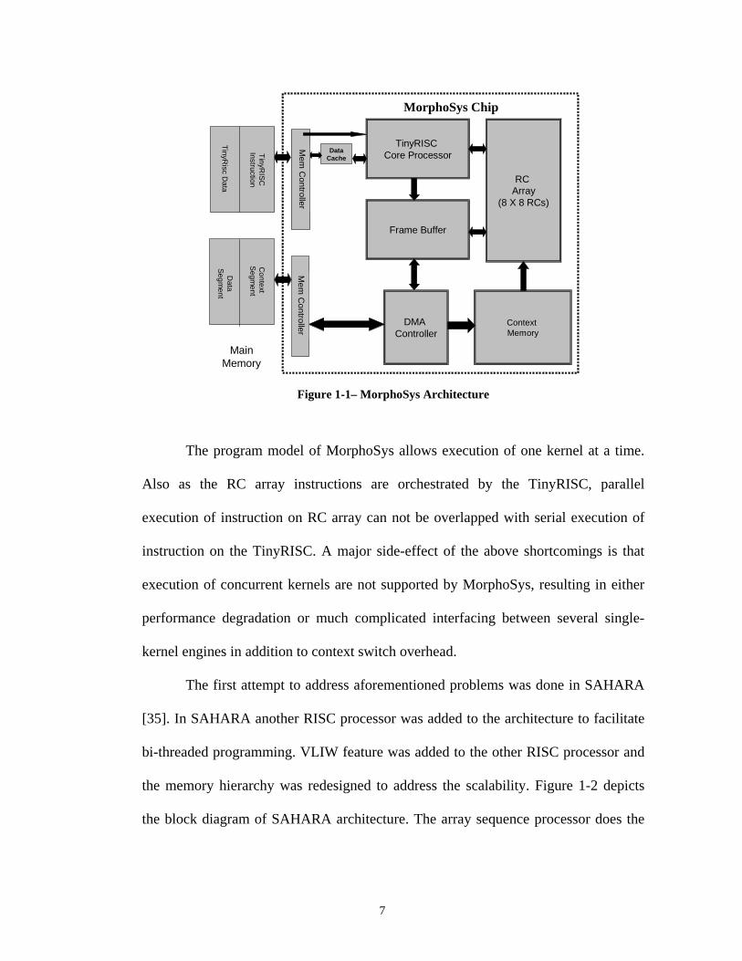
A block diagram of MorphoSys architecture is shown in Figure 1-1.
TinyRISC is a simple processor in charge of the sequential part of the algorithm in
addition to orchestrating the whole core. The parallel and computation intensive
portion of a task is performed on an array of Reconfigurable Cells (RC Array). RC
6
array is an 8x8 array of simple processing unit (integer ALU, MAC and SRAM) and
the programming model is SIMD.
The problem with MorphoSys is that it is not scalable with respect to array
size and technology, as it uses long wires. Data and instruction broadcast to the RC
array, and also some inter-RC communication in this processor are performed over
global buses. However, this type of signal path cannot easily be scaled as our
hypothetical MorphoSys utilizes larger RC arrays. Even in the current versions long
buses have to be considered thoroughly, and are usually the major sources of design
backtracking to meet the timing constraint. In fact, wire delay is becoming a major
constraint in the implementation of large processors, so that while wires used to
interconnect logic gates in the past, today the situation is being reversed: wires are
said to be interconnected by logic gates. Therefore, generous use of wires is no longer
consistent with modern, high performance massively parallel processors.
Moreover, memory hierarchy in MorphoSys has to be improved for the
growing RC array, as a centralized data memory and a centralized instruction
memory cannot efficiently exploit the possible spatial and temporal localities.
Furthermore, the current off-chip memory bandwidth is a rigid bottleneck for non-
streaming data intensive applications, such as the BSP-based ray tracing [34].
7
TinyRISC Core Processor
Context Memory
RC Array
(8 X 8 RCs)
DMA Controller
Data Cache
TinyR
ISC
Instruction
TinyR
iscD
ata
Mem
Controller
Main Memory
Frame Buffer
Context
Seg
ment
Data
Seg
ment
Mem
Controller
MorphoSys Chip
Figure 1-1– MorphoSys Architecture
The program model of MorphoSys allows execution of one kernel at a time.
Also as the RC array instructions are orchestrated by the TinyRISC, parallel
execution of instruction on RC array can not be overlapped with serial execution of
instruction on the TinyRISC. A major side-effect of the above shortcomings is that
execution of concurrent kernels are not supported by MorphoSys, resulting in either
performance degradation or much complicated interfacing between several single-
kernel engines in addition to context switch overhead.
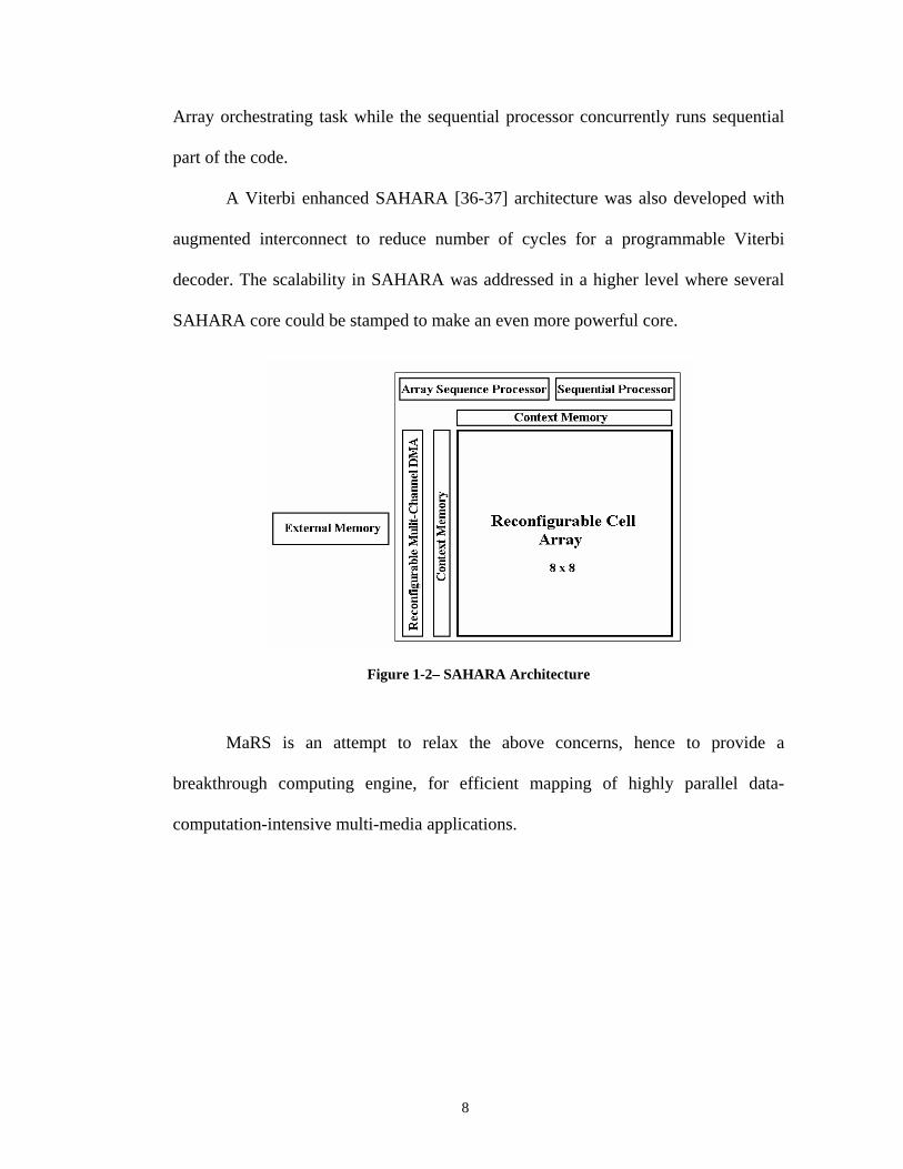
The first attempt to address aforementioned problems was done in SAHARA
[35]. In SAHARA another RISC processor was added to the architecture to facilitate
bi-threaded programming. VLIW feature was added to the other RISC processor and
the memory hierarchy was redesigned to address the scalability. Figure 1-2 depicts
the block diagram of SAHARA architecture. The array sequence processor does the
8
Array orchestrating task while the sequential processor concurrently runs sequential
part of the code.
A Viterbi enhanced SAHARA [36-37] architecture was also developed with
augmented interconnect to reduce number of cycles for a programmable Viterbi
decoder. The scalability in SAHARA was addressed in a higher level where several
SAHARA core could be stamped to make an even more powerful core.
Figure 1-2– SAHARA Architecture
MaRS is an attempt to relax the above concerns, hence to provide a
breakthrough computing engine, for efficient mapping of highly parallel data-
computation-intensive multi-media applications.
9
Chapter 2 MaRS Architecture
MaRS Architecture
MaRS is an array of simple processing elements connected together using a
network-on-chip methodology, targeting computation intensive applications. The
micro-architecture and ISA of MaRS are discussed in this Chapter.
2.1 Top-level Architecture View
MaRS is a 2-D array of small coarse grain processing elements (PE)
connected together using a mesh network (please note the transition from
Reconfigurable Cell to the more widely used Processing Element term in MaRS).
The architecture is potentially heterogeneous i.e. different type of PEs can
exist. Therefore the architecture can be customized by choosing different PEs from
the library. The library currently features a standard floating point unit (FPU), an
efficient bi-tonic sorter with application in cognitive sciences [38] and trellis traversal
part of Viterbi algorithm, which is explained in detail in Chapter 6. Some other good
candidates are complex correlation units and turbo decoder for wireless applications.
The application specific PEs use the same routing algorithm to communicate with
other PEs.
10
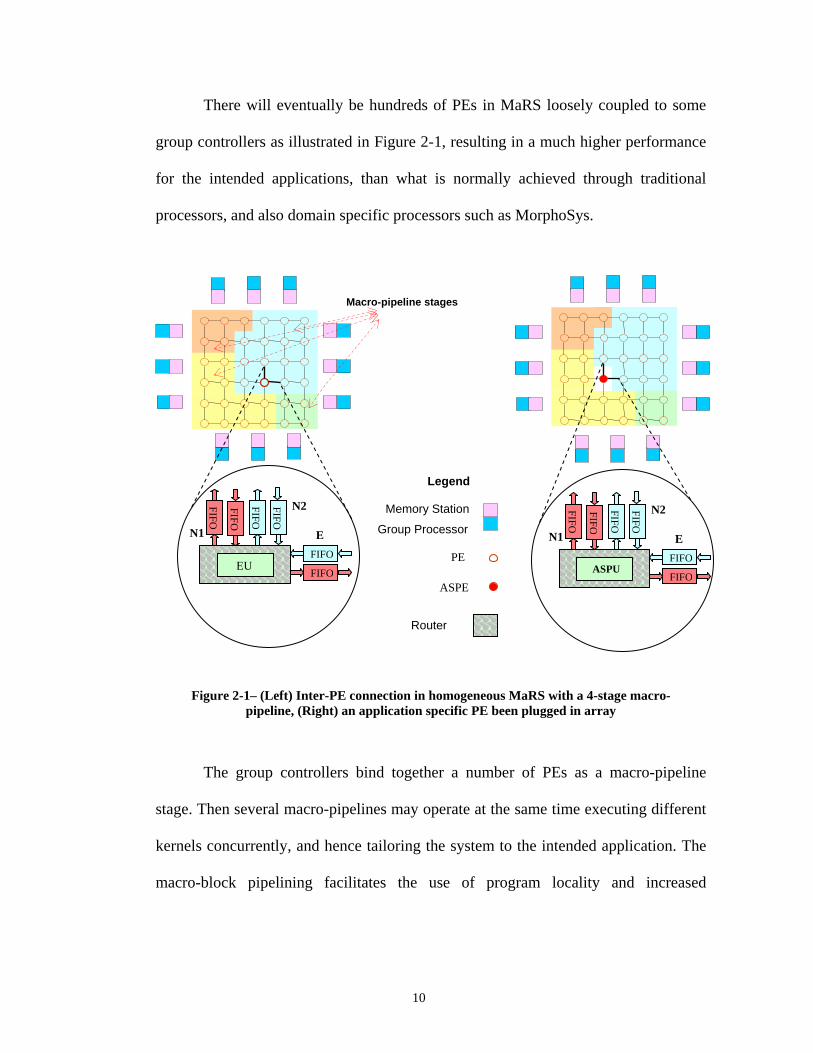
There will eventually be hundreds of PEs in MaRS loosely coupled to some
group controllers as illustrated in Figure 2-1, resulting in a much higher performance
for the intended applications, than what is normally achieved through traditional
processors, and also domain specific processors such as MorphoSys.
Figure 2-1– (Left) Inter-PE connection in homogeneous MaRS with a 4-stage macro-pipeline, (Right) an application specific PE been plugged in array
The group controllers bind together a number of PEs as a macro-pipeline
stage. Then several macro-pipelines may operate at the same time executing different
kernels concurrently, and hence tailoring the system to the intended application. The
macro-block pipelining facilitates the use of program locality and increased
N1
N2 FIF
O
FIF
O
FIF
O
FIF
O
EU FIFO
E
FIFO
Macro-pipeline stages
N1
N2 FIF
O
FIF
O
FIF
O
FIF
O
ASPU FIFO
E
FIFO
Legend Memory Station
Group Processor
ASPE
Router
PE

11
throughput. An example of several kernels working in a macro pipeline fashion is
shown in Figure 2-2.
Figure 2-2– Macro-pipeline model on MaRS
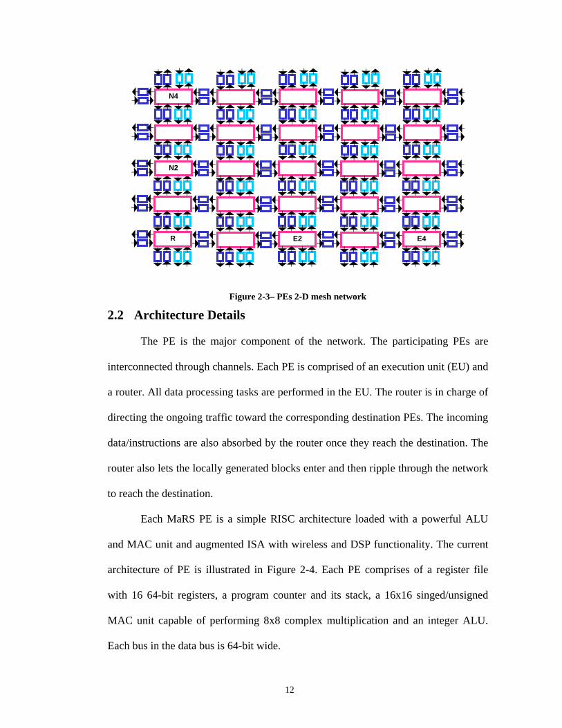
Each PE in MaRS array is a 32-bit datapath. Each PE is connected to its four
neighboring PEs through 12 FIFOs as shown in Figure 2-3 using a deadlock-free
minimal routing protocol. The number of PEs is implementation dependent. The
network supports point-to-point single-word and also point-to-point/multicast block
transfer between any two PEs.
Kernel2
Kernel4
Kernel3 Kernel1
12
Figure 2-3– PEs 2-D mesh network
2.2 Architecture Details
The PE is the major component of the network. The participating PEs are
interconnected through channels. Each PE is comprised of an execution unit (EU) and
a router. All data processing tasks are performed in the EU. The router is in charge of
directing the ongoing traffic toward the corresponding destination PEs. The incoming
data/instructions are also absorbed by the router once they reach the destination. The
router also lets the locally generated blocks enter and then ripple through the network
to reach the destination.
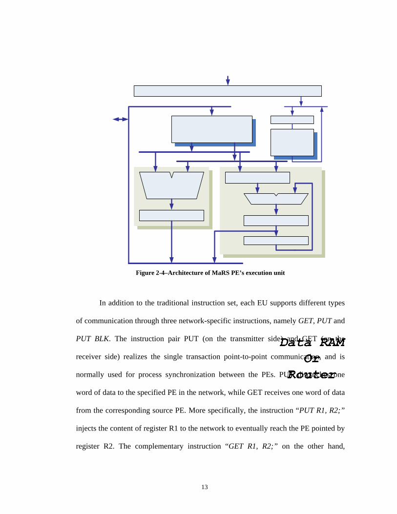
Each MaRS PE is a simple RISC architecture loaded with a powerful ALU
and MAC unit and augmented ISA with wireless and DSP functionality. The current
architecture of PE is illustrated in Figure 2-4. Each PE comprises of a register file
with 16 64-bit registers, a program counter and its stack, a 16x16 singed/unsigned
MAC unit capable of performing 8x8 complex multiplication and an integer ALU.
Each bus in the data bus is 64-bit wide.
N4
E4 E2 R
N2
13
Figure 2-4–Architecture of MaRS PE’s execution unit
In addition to the traditional instruction set, each EU supports different types
of communication through three network-specific instructions, namely GET, PUT and
PUT BLK. The instruction pair PUT (on the transmitter side) and GET (on the
receiver side) realizes the single transaction point-to-point communication, and is
normally used for process synchronization between the PEs. PUT dispatches one
word of data to the specified PE in the network, while GET receives one word of data
from the corresponding source PE. More specifically, the instruction “PUT R1, R2;”
injects the content of register R1 to the network to eventually reach the PE pointed by
register R2. The complementary instruction “GET R1, R2;” on the other hand,

14
receives a word from the PE pointed by register R2. R1 is the destination register.
Notice that due to possible network congestion and also unknown instant of
instruction fetch, both PUT and GET have a nondeterministic period of execution
cycle.
The GET instruction is bound to the corresponding PUT instruction; that is,
the former has to wait until the required data arrives. In case of an early arrival, the
data is temporarily saved in a content addressable memory (CAM), and then upon the
execution of the GET instruction the right data is located and fetched from the CAM.
This mechanism also supports multiple early arrivals.
The “PUT BLK R1;” instruction initiates the transfer of up to 1k-byte blocks,
leaving the local RAM of the source PE, or a memory station, and heading to the
local RAM of the destination PE, or a memory station in point-to-point (one-to-one)
block transfers, or the local RAMs of a group of PEs in multicast (one-to-many)
mode. Register R1 points to the beginning of the block in the source RAM.
Instruction blocks, of course, are not allowed to leave instruction RAMs as they
normally flow from the memory stations towards the local instruction RAMs in
different PEs. Multicast mode results in a significant saving in power dissipation
comparing to the equivalent multiple point-to-point block transfers by eliminating
redundant packet transportations. In this mode the destination PEs (a macro-block)
may be specified and arranged in an arbitrary shape. According to our current
implementation, a macro-block may be comprised of a stack of up to four 8- by 8-PE
(or smaller) rectangles, with an indentation of up to 7 PEs for each rectangle. Figure
2-5 shows a multicast to a 4-rectangle macro-block, initiated from a memory station.

15
The values in parentheses show the corresponding vertex coordinates to be specified
in the header. For each rectangle two vertices located on the left-to-right diagonal
have to be specified.
Figure 2-5–A multicast to a 4-rectangle macro-block
Upon the power-on-reset, each EU is forced to execute a single-instruction
wait loop until an instruction block reaches the instruction RAM. Then the execution
path will be redirected towards the newly received block of code. Considering that
instruction pumping into the network during an instruction-block transfer by a
memory station may not be interrupted once the block header has reached the
destination, the PE does not have to wait for the end of instruction-block transfer to
begin execution. In order to leave the PE in a waiting situation when the execution of
a piece of code is over, MaRS features a software reset instruction, HALT, to be used
at the logical end of programs. The HALT instruction forces the EU to enter the same
single-instruction wait loop again.
Memory Station
PE Array
H(2,1)
G(2,0)
F(4,2)
E(1,0)
D(3,0) C(3,0)
B(2,1)
A(2,0)
16
2.2.1 Routers and Channels
The way the processing elements are connected to one another varies among
different architectures. In direct network architecture, each node has a point-to-point,
or direct, connection to some number of other nodes, called neighboring nodes. Direct
networks have become a popular architecture for constructing massively parallel
computers because they scale well; that is, as the number of nodes in the system
increases, the total communication bandwidth, memory bandwidth, and processing
capability of the system also increase.
AS the PEs do not share physical memory, nodes must communicate by
passing messages through the network. Message size may vary, depending on the
application. For efficient and fair use of network resources, a message is often
divided into packets prior to transmission. A packet is the smallest unit of
communication that contains routing and sequencing information; this information is
carried in the packet header. Neighboring nodes may send packets to one another
directly, while nodes that are not directly connected must rely on other nodes in the
network to relay packets from source to destination. In many systems, each PE
contains a separate router to handle such communication-related tasks. Although a
router’s function could be performed by the corresponding local processor, dedicated
routers are used to allow overlapped computation and communication within each
node.
By connecting the input channels of one node to the output channels of other
nodes, the topology of the direct network is defined. A packet sent between two nodes
that are not neighboring must be forwarded by routers along multiple external
17
channels. Usually, a crossbar is used to allow all possible connections between the
input and output channels within the router. The sequential list of channels traversed
by such a packet is called a path, and the number of channels in the path is called the
path length.
A variety of switching techniques have been used in direct networks. One
method, called wormhole routing, has become quite popular in recent years. By its
nature, wormhole routing is particularly susceptible to deadlock situations, in which
two or more packets may block one another indefinitely. Deadlock avoidance is
usually guaranteed by the routing algorithm, which selects the path a packet takes.
A 64-bit (double-word) 2D-mesh communication network with adaptive,
wormhole, and deadlock-free routing is developed and implemented for MaRS.
Figure 2-3 illustrates how individual PEs/FPUs are interconnected to their
neighboring FPUs/PEs through 6 input and 6 output channels.
There are two north and two south channel pairs reaching each router,
providing two disjoint sub-networks for the west-to-east and east-to-west traffics
using the channel sets W-in, N1, E-out, S1 and E-in, N2, W-out, S2,
respectively. This allows the network avoid cycles in its channel-dependency-graph,
resulting in a deadlock-free operation [39]. Each channel is comprised of a 4-double-
word FIFO, and the corresponding sets of physical wires.
As soon as an outgoing channel is allocated to a double-word header, the
channel will remain dedicated to the corresponding block until the tail end of the
block passes through the channel. This guarantees that an instruction block leaving a
memory station will not be interrupted once the header has reached the destination.
18
However, that is not true for data-block transfers initiated by a PE in our
implementation, as an incoming data block heading to the same node does stop the
outgoing data transfer already in progress.
Notice that in single transactions no block body follows the header. Now in
fact a 32-bit header (short header) is appended to the 32-bit data. The resulting
double-word data/header then ripples through the network exactly in the same way
that a 64-bit header does in a point-to-point block transfer.
The route traversed by a block header is nondeterministic, as each header
adapts its direction to the current situation while stepping from one node to a
neighboring node. For outgoing channel allocation the router applies a fixed priority
scheme to the incoming headers reached the corresponding node simultaneously: for
each outgoing channel, the possible incoming channels have a descending order of
priority in a clock-wise direction. For example, for the outgoing channel W, the
channels N2, E and S2 are the three possible incoming channels in descending order
of priority.
In addition to the above four incoming channels, there are two more sources
requesting an outgoing channel in each node, namely the local RAM when a PUT
BLK instruction is executed, and the execution unit when a PUT instruction is
executed. The lowest and the second lowest priority are allocated respectively to
these two sources in our current implementation.
Notice that the route traversed during a block transfer is strictly monotonic; in
other words for each incoming header there are at most two logically possible
outgoing channels, always resulting in a minimal route. If the first-choice outgoing
19
channel cannot be allocated to a header, the second choice (if any) will be granted if it
has not already been dedicated, and there is no priority violation either.
2.2.2 FPU
Any of the participating PEs may be replaced with a floating point unit (FPU)
in MaRS, leading to a heterogeneous architecture. The distributed FPUs utilized in
MaRS provide additional support for multimedia processing, yet real-estate overhead
due to floating-point-enabled PEs is avoided.
Each added FPU is able to provide any PE in the network with the requested
floating-point service using the same network protocol, while the FPU remains
transparent to the ongoing traffic in the network. Each FPU is also comprised of a
router (FP-router) and an execution unit (FPEU), as articulated in the following
subsections.
2.2.2.1 FPEU
The FPEU supports the IEEE 754-based single precision floating-point
addition, subtraction, and multiplication. In the current implementation FPEU is a
multi-cycle unit. Its pipelined version will be utilized in the upcoming
implementations of MaRS. Notice that all supported floating-point operations need
32-bit operands, and therefore one double-word block transfer by the requesting PE
suffices to provide the FPEU with both of the operands. The operation type and the
source/destination addresses are transmitted in the block header. As soon as the
computation is carried out, a single transaction is initiated by the FPEU’s controller
to dispatch the 32-bit result to the requesting PE. The matching GET instruction on
20
the PE side will receive the operation result. Notice that there is no local instruction
or data RAM in the FPEU.
2.2.2.2 FP-router
The FP-router is still in charge of routing the ongoing traffic, which reaches
the corresponding FPU. Furthermore, all floating-point requests and the
computation results are directed by this router. Notice that the incoming blocks to a
FPU are handled differently. These requests enter a floating-point FIFO (instead of
the local RAM) in the FPU, and then are served on a first-in first-served basis. Due
to the non-pipelined and multi-cycle architecture of the FPEU the floating-point
FIFO is likely to become full under heavy load conditions. There are two more
major changes to the FP-router; there is no outgoing block transfer from this router,
and since the FPU cannot be a destination for a multicast the FP-router simply
ignores all such requests.
2.3 The Second Layer of Inter-PE Connections
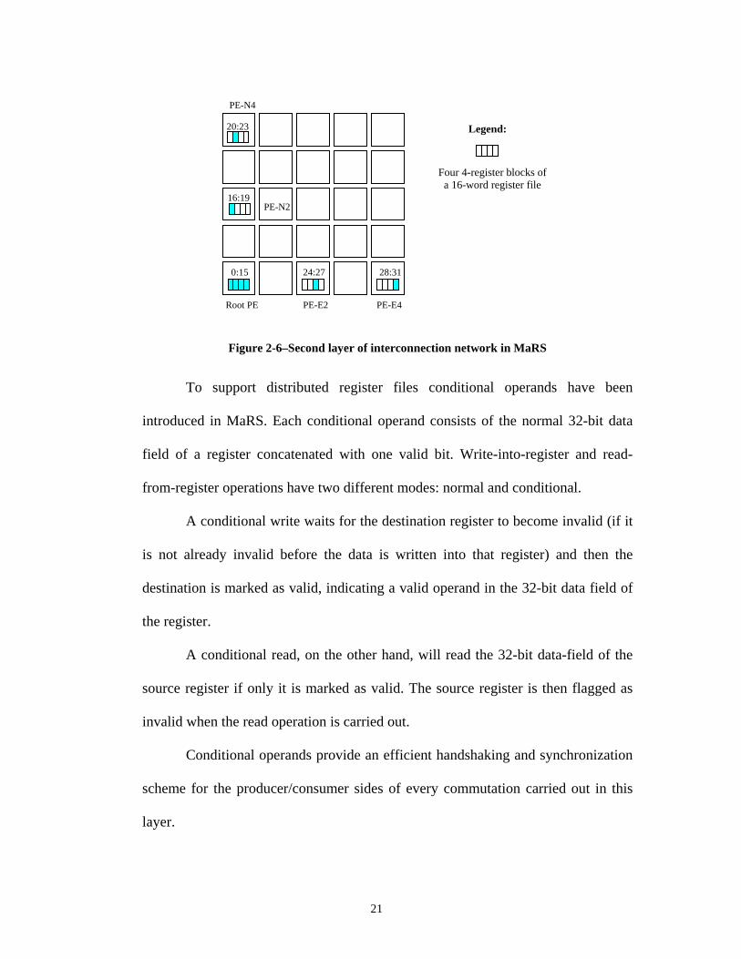
As a second layer of interconnection network, distributed shared register file
has been incorporated in MaRS, providing a tightly coupled array of PEs required
by the communication-intensive in DSP and wireless communication such as
Viterbi decoder and FFT. In the current implementation of MaRS, half of the 32-
word register file of each PE (the root PE: ‘R’) is distributed in four remote PEs,
namely N2, N4, E2, and E4, as shown in Figure 2-6, facilitating much faster inter-
PE communication. It can also realize different sizes of the ‘exchange’ network,
which has been proved to be a common communication pattern for signal
processing applications [40].
21
Figure 2-6–Second layer of interconnection network in MaRS
To support distributed register files conditional operands have been
introduced in MaRS. Each conditional operand consists of the normal 32-bit data
field of a register concatenated with one valid bit. Write-into-register and read-
from-register operations have two different modes: normal and conditional.
A conditional write waits for the destination register to become invalid (if it
is not already invalid before the data is written into that register) and then the
destination is marked as valid, indicating a valid operand in the 32-bit data field of
the register.
A conditional read, on the other hand, will read the 32-bit data-field of the
source register if only it is marked as valid. The source register is then flagged as
invalid when the read operation is carried out.
Conditional operands provide an efficient handshaking and synchronization
scheme for the producer/consumer sides of every commutation carried out in this
layer.
Legend:
Four 4-register blocks of a 16-word register file
PE-E4
PE-E2
28:31
24:27
PE-N4
Root PE
20:23
0:15
16:19 PE-N2

22
For example the instruction ADD R27c, R17, R29c with a conditional read
from register R29 (signified by the suffix “c”), and a conditional write into register
R27 (signified again by the suffix “c”), waits until registers R29 and R27 become
valid and invalid respectively, and then saves the result of R17 + R29 into R27,
while R29 and R27 are flagged as invalid, and valid respectively.
Notice that in addition to a higher throughput, the conditional read/write
operations provide the participating PEs with a fast and straightforward
handshaking and synchronization mechanism as well.
The valid bit is totally ignored in normal-mode read operations; that is, the
read operation is performed unconditionally, and the corresponding valid bit
remains unchanged after such a read. Write operation, on the other hand, is still
subject to an invalid destination. However, the destination remains invalid after
such a write.
In the current implementation of MaRS each block of remote registers
(located in one remote PE) allows only one access at a time, however, three remote
registers in three different remote blocks may be accessed simultaneously by the
root PE.
2.4 Accelerator for Viterbi Decoding
Viterbi decoding is a kernel that has been used in most of the wireless
standards. In order to enhance the performance of the architecture for Viterbi and
turbo decoding, each PE’s ALU has an Add-Compare-Select (ACS) unit. The soft
decision Viterbi decoding algorithm will be discussed in details in Chapters 4 and 6.
The ACS unit is capable of performing a half butterfly ACS operation.
23
2.5 Instruction Set Architecture
MaRS processing elements support a simple RISC ISA with some added
instructions for the target applications. Currently, each instruction is 32 bits.
Instructions can be divided into different groups. The PE is designed in advanced
computer architecture element and the MorphoSys reconfigurable cell architecture
datapath is used to reduce the design cycle as well. For a detailed list of ISA and
flags please refer to Appendix A.
2.6 MaRS RTL Implementation
MaRS is implemented using synthesizable VHDL code. Artisan [41]
memory generator has been used to implement memory and registers. Major blocks
of MaRS have been synthesized in a 0.13µm standard CMOS process using artisan
standard cell libraries, followed by some successful post-synthesis simulations. The
timing closure based on 2.2 nsec has been successfully achieved for MaRS leading
to a maximum clock frequency of 450 MHz.

24
Chapter 3 MaRS Programming Model & Applications
MaRS Programming Model & Applications
MorphoSys programming model was SIMD which was a limitation. In order
to make the architecture more general for a wider range of applications, MaRS uses
PEs running different programs each with independent program counters. This
makes the architecture to be capable of using data level parallelism, task level
parallelism, thread level parallelism finally macro-block pipelining.
3.1 Parallel Programming on MaRS
A baseband processing part of a wireless/multimedia system is divided into
different macro-blocks working in a producer consumer chain. In choosing macro-
blocks, one should consider the following facts:
• Macro-pipeline stages be as balanced as possible
• The tasks of same nature be in same macro-block
• Maximum data locality be utilized
Once the macro-blocks decision is made, each task should be partitioned
into many parallel tasks running concurrently on different PEs. Synchronization is
25
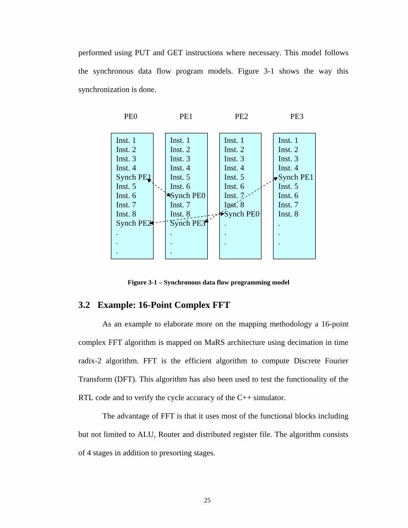
performed using PUT and GET instructions where necessary. This model follows
the synchronous data flow program models. Figure 3-1 shows the way this
synchronization is done.
Figure 3-1 – Synchronous data flow programming model
3.2 Example: 16-Point Complex FFT
As an example to elaborate more on the mapping methodology a 16-point
complex FFT algorithm is mapped on MaRS architecture using decimation in time
radix-2 algorithm. FFT is the efficient algorithm to compute Discrete Fourier
Transform (DFT). This algorithm has also been used to test the functionality of the
RTL code and to verify the cycle accuracy of the C++ simulator.
The advantage of FFT is that it uses most of the functional blocks including
but not limited to ALU, Router and distributed register file. The algorithm consists
of 4 stages in addition to presorting stages.
PE0 PE1 PE2 PE3
Inst. 1 Inst. 2 Inst. 3 Inst. 4 Synch PE1 Inst. 5 Inst. 6 Inst. 7 Inst. 8 Synch PE2 . . .
Inst. 1 Inst. 2 Inst. 3 Inst. 4 Inst. 5 Inst. 6 Synch PE0 Inst. 7 Inst. 8 Synch PE3 . . .
Inst. 1 Inst. 2 Inst. 3 Inst. 4 Inst. 5 Inst. 6 Inst. 7 Inst. 8 Synch PE0 . . .
Inst. 1 Inst. 2 Inst. 3 Inst. 4 Synch PE1 Inst. 5 Inst. 6 Inst. 7 Inst. 8 . . .

26
3.2.1 FFT Algorithm
DFT is formulated as:
∑−
=
−==1
0
1,...,1,0,][][N
n
knN NkWnxkX where )/2( Nj
N eW π−= Equation 3-1
Direct computation of DFT incorporates a lot of complex multiplication and
addition operations. FFT algorithms have been proposed to reduce the number of
required multiplications from O(N2) to O(NLog(N)). In order to achieve such a
speed-up, algorithms usually use the symmetry and periodicity of KnNW . This
reduction results from decomposing DFT into successively smaller DFT sizes. This
decomposition can be done to all prime factors of the DFT size, as it is known as
Cooley-Tukey algorithm [42]. The decomposition value for each stage is called the
radix for that stage. A very popular case is when the FFT size is a power of 2 where
cascaded radix-2 stages are used. Using radix-4 stages will reduce number of stages
but each stage would be more complicated and needs more data communication.
Let’s assume that computation of DFT of size N=2v is desired. Since N is an
even integer we can consider computing X[k] by separating x[n] into two (N/2)-
point sequences consisting of the even numbered points in x[n]and the odd
numbered pints in x[n] . With X[k] given by
1,...,1,0,][][1
0
−==∑−
=
NkWnxkXN
n
nkN Equation 3-2
And by separating x[n] into its even and odd numbered points, we get
∑∑−−
+=oddn
nkN
evenn
nkN WnxWnxkX ][][][ Equation 3-3
With the substitution of n=2r for n even and n=2r+1 for n odd we obtain
27
∑∑
∑∑−
=
−
=
−
=
+−
=
++=
++=
1)2/(
0
21)2/(
0
2
1)2/(
0
)12(1)2/(
0
2
)](12[)](2[
]12[]2[][
N
r
rkN
kN
N
r
rkN
N
r
krN
N
r
rkN
WrxWWrx
WrxWrxkX
Equation 3-4
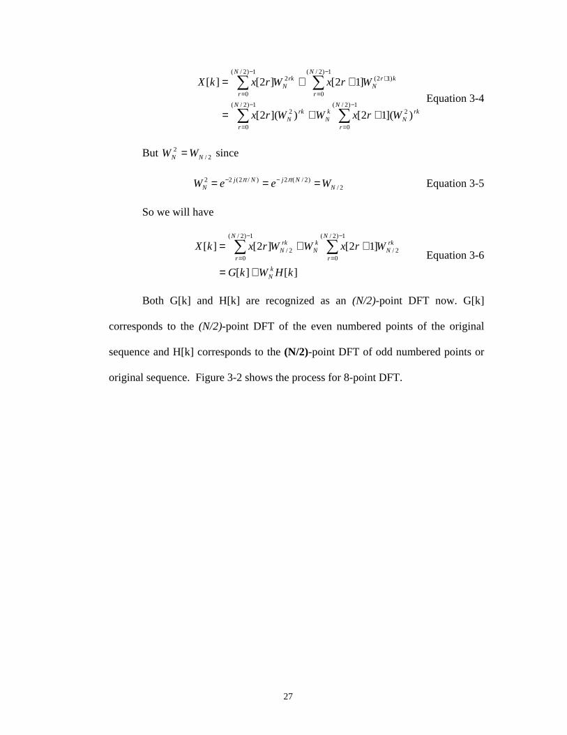
But 2/2
NN WW = since
2/)2/(2)/2(22
NNjNj
N WeeW === −− ππ Equation 3-5
So we will have
][][
]12[]2[][1)2/(
02/
1)2/(
02/
kHWkG
WrxWWrxkX
kN
N
r
rkN
kN
N
r
rkN
+=
++= ∑∑−
=
−
= Equation 3-6
Both G[k] and H[k] are recognized as an (N/2)-point DFT now. G[k]
corresponds to the (N/2)-point DFT of the even numbered points of the original
sequence and H[k] corresponds to the (N/2)-point DFT of odd numbered points or
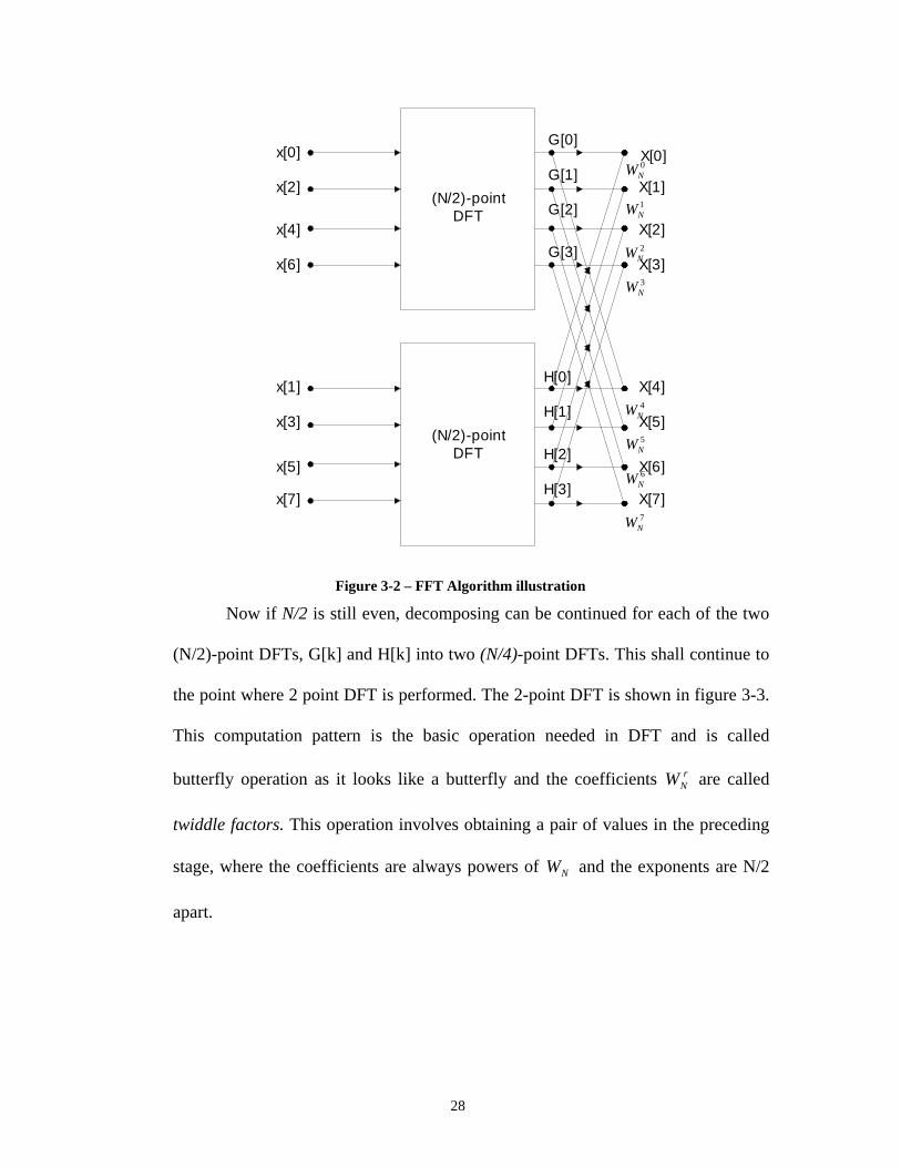
original sequence. Figure 3-2 shows the process for 8-point DFT.
28
x[0]
x[2]
x[4]
x[6]
x[1]
x[3]
x[5]
x[7]
(N/2)-pointDFT
(N/2)-pointDFT
X[0]
X[1]
X[2]
X[3]
G[0]
X[6]
X[5]
X[4]
X[7]
G[3]
G[2]
G[1]
H[0]
H[1]
H[2]
H[3]
0NW
1NW
2NW
3NW
4NW
5NW
6NW
7NW
Figure 3-2 – FFT Algorithm illustration
Now if N/2 is still even, decomposing can be continued for each of the two
(N/2)-point DFTs, G[k] and H[k] into two (N/4)-point DFTs. This shall continue to
the point where 2 point DFT is performed. The 2-point DFT is shown in figure 3-3.
This computation pattern is the basic operation needed in DFT and is called
butterfly operation as it looks like a butterfly and the coefficients rNW are called
twiddle factors. This operation involves obtaining a pair of values in the preceding
stage, where the coefficients are always powers of NW and the exponents are N/2
apart.

29
(m-1)thstage
mthstage
rNW
)2/( NrNW +
Figure 3-3 – 2-point DFT butterfly
Since rN
rN
NN
NrN WWWW −==+ 2/2/ the butterfly can be further reduced to
Figure 3-4 where one complex multiplication is required instead of two.
(m-1)thstage
mthstage
rNW 1−
Figure 3-4 – Simplified 2-point DFT butterfly
3.2.2 Mapping FFT
Assumption here is that an array of 2x2 is used for this mapping. It is also
assumed that the instructions and data are already loaded inside each PE.
Transferring data and instruction to PEs is performed by injecting them from
memory stations and using correct headers. Data is assumed to be in registers R0-
R3 of each PE. Figure 3-2 illustrates the way PEs are laid out on the array. The X
and Y values are used in the routing network header. In the configuration shown
below the arrow means increasing X and Y. Therefore in order to go from PE00 to
PE11 X=1 and Y=1 should be taken, or from PE01 to PE10 X=-1 and Y=-1 should
be taken. The PUT and GET instruction in the code use these directions. It should
be noted that the negative values are represented in 2’s complement format.

30
Figure 3-5 – Layout of PEs in the array
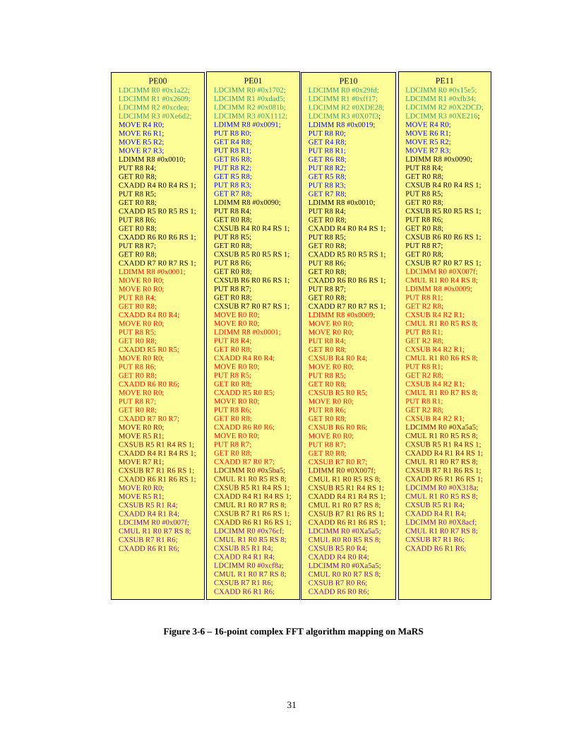
Figure 3-6 shows the code for each MaRS PE to perform the FFT
algorithm. Explanation and clarification of the code follows the diagram. In order to
get a better understanding of the code, color coding is used. In the diagram, the
green color shows the data loading part and blue color represents the presorting step
of the algorithm. Each stage of the algorithm is shown with a distinct color as well.
PE00 PE01
PE10 PE11
X axis in routing network
Y a
xis
in r
ou
ting
net
wor
k
31
Figure 3-6 – 16-point complex FFT algorithm mapping on MaRS
PE00 LDCIMM R0 #0x1a22; LDCIMM R1 #0x2609; LDCIMM R2 #0xcdea; LDCIMM R3 #0Xe6d2; MOVE R4 R0; MOVE R6 R1; MOVE R5 R2; MOVE R7 R3; LDIMM R8 #0x0010; PUT R8 R4; GET R0 R8; CXADD R4 R0 R4 RS 1; PUT R8 R5; GET R0 R8; CXADD R5 R0 R5 RS 1; PUT R8 R6; GET R0 R8; CXADD R6 R0 R6 RS 1; PUT R8 R7; GET R0 R8; CXADD R7 R0 R7 RS 1; LDIMM R8 #0x0001; MOVE R0 R0; MOVE R0 R0; PUT R8 R4; GET R0 R8; CXADD R4 R0 R4; MOVE R0 R0; PUT R8 R5; GET R0 R8; CXADD R5 R0 R5; MOVE R0 R0; PUT R8 R6; GET R0 R8; CXADD R6 R0 R6; MOVE R0 R0; PUT R8 R7; GET R0 R8; CXADD R7 R0 R7; MOVE R0 R0; MOVE R5 R1; CXSUB R5 R1 R4 RS 1; CXADD R4 R1 R4 RS 1; MOVE R7 R1; CXSUB R7 R1 R6 RS 1; CXADD R6 R1 R6 RS 1; MOVE R0 R0; MOVE R5 R1; CXSUB R5 R1 R4; CXADD R4 R1 R4; LDCIMM R0 #0x007f; CMUL R1 R0 R7 RS 8; CXSUB R7 R1 R6; CXADD R6 R1 R6;
PE01 LDCIMM R0 #0x1702; LDCIMM R1 #0xdad5; LDCIMM R2 #0x081b; LDCIMM R3 #0X1112; LDIMM R8 #0x0091; PUT R8 R0; GET R4 R8; PUT R8 R1; GET R6 R8; PUT R8 R2; GET R5 R8; PUT R8 R3; GET R7 R8; LDIMM R8 #0x0090; PUT R8 R4; GET R0 R8; CXSUB R4 R0 R4 RS 1; PUT R8 R5; GET R0 R8; CXSUB R5 R0 R5 RS 1; PUT R8 R6; GET R0 R8; CXSUB R6 R0 R6 RS 1; PUT R8 R7; GET R0 R8; CXSUB R7 R0 R7 RS 1; MOVE R0 R0; MOVE R0 R0; LDIMM R8 #0x0001; PUT R8 R4; GET R0 R8; CXADD R4 R0 R4; MOVE R0 R0; PUT R8 R5; GET R0 R8; CXADD R5 R0 R5; MOVE R0 R0; PUT R8 R6; GET R0 R8; CXADD R6 R0 R6; MOVE R0 R0; PUT R8 R7; GET R0 R8; CXADD R7 R0 R7; LDCIMM R0 #0x5ba5; CMUL R1 R0 R5 RS 8; CXSUB R5 R1 R4 RS 1; CXADD R4 R1 R4 RS 1; CMUL R1 R0 R7 RS 8; CXSUB R7 R1 R6 RS 1; CXADD R6 R1 R6 RS 1; LDCIMM R0 #0x76cf; CMUL R1 R0 R5 RS 8; CXSUB R5 R1 R4; CXADD R4 R1 R4; LDCIMM R0 #0xcf8a; CMUL R1 R0 R7 RS 8; CXSUB R7 R1 R6; CXADD R6 R1 R6;
PE10 LDCIMM R0 #0x29fd; LDCIMM R1 #0xff17; LDCIMM R2 #0XDE28; LDCIMM R3 #0X07f3; LDIMM R8 #0x0019; PUT R8 R0; GET R4 R8; PUT R8 R1; GET R6 R8; PUT R8 R2; GET R5 R8; PUT R8 R3; GET R7 R8; LDIMM R8 #0x0010; PUT R8 R4; GET R0 R8; CXADD R4 R0 R4 RS 1; PUT R8 R5; GET R0 R8; CXADD R5 R0 R5 RS 1; PUT R8 R6; GET R0 R8; CXADD R6 R0 R6 RS 1; PUT R8 R7; GET R0 R8; CXADD R7 R0 R7 RS 1; LDIMM R8 #0x0009; MOVE R0 R0; MOVE R0 R0; PUT R8 R4; GET R0 R8; CXSUB R4 R0 R4; MOVE R0 R0; PUT R8 R5; GET R0 R8; CXSUB R5 R0 R5; MOVE R0 R0; PUT R8 R6; GET R0 R8; CXSUB R6 R0 R6; MOVE R0 R0; PUT R8 R7; GET R0 R8; CXSUB R7 R0 R7; LDIMM R0 #0X007f; CMUL R1 R0 R5 RS 8; CXSUB R5 R1 R4 RS 1; CXADD R4 R1 R4 RS 1; CMUL R1 R0 R7 RS 8; CXSUB R7 R1 R6 RS 1; CXADD R6 R1 R6 RS 1; LDCIMM R0 #0Xa5a5; CMUL R0 R0 R5 RS 8; CXSUB R5 R0 R4; CXADD R4 R0 R4; LDCIMM R0 #0Xa5a5; CMUL R0 R0 R7 RS 8; CXSUB R7 R0 R6; CXADD R6 R0 R6;
PE11 LDCIMM R0 #0x15e5; LDCIMM R1 #0xfb34; LDCIMM R2 #0X2DCD; LDCIMM R3 #0XE216; MOVE R4 R0; MOVE R6 R1; MOVE R5 R2; MOVE R7 R3; LDIMM R8 #0x0090; PUT R8 R4; GET R0 R8; CXSUB R4 R0 R4 RS 1; PUT R8 R5; GET R0 R8; CXSUB R5 R0 R5 RS 1; PUT R8 R6; GET R0 R8; CXSUB R6 R0 R6 RS 1; PUT R8 R7; GET R0 R8; CXSUB R7 R0 R7 RS 1; LDCIMM R0 #0X007f; CMUL R1 R0 R4 RS 8; LDIMM R8 #0x0009; PUT R8 R1; GET R2 R8; CXSUB R4 R2 R1; CMUL R1 R0 R5 RS 8; PUT R8 R1; GET R2 R8; CXSUB R4 R2 R1; CMUL R1 R0 R6 RS 8; PUT R8 R1; GET R2 R8; CXSUB R4 R2 R1; CMUL R1 R0 R7 RS 8; PUT R8 R1; GET R2 R8; CXSUB R4 R2 R1; LDCIMM R0 #0Xa5a5; CMUL R1 R0 R5 RS 8; CXSUB R5 R1 R4 RS 1; CXADD R4 R1 R4 RS 1; CMUL R1 R0 R7 RS 8; CXSUB R7 R1 R6 RS 1; CXADD R6 R1 R6 RS 1; LDCIMM R0 #0X318a; CMUL R1 R0 R5 RS 8; CXSUB R5 R1 R4; CXADD R4 R1 R4; LDCIMM R0 #0X8acf; CMUL R1 R0 R7 RS 8; CXSUB R7 R1 R6; CXADD R6 R1 R6;
32
The coded loads the registers with 16 bit complex values (8-bit real and 8-
bit imaginary input data. The twiddle factors are passed to the code as immediate
operands. The first two stages need inter-PE communication while stages 3 and 4
use the data locally in the PE.
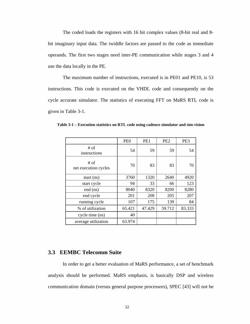
The maximum number of instructions, executed is in PE01 and PE10, is 53
instructions. This code is executed on the VHDL code and consequently on the
cycle accurate simulator. The statistics of executing FFT on MaRS RTL code is
given in Table 3-1.
Table 3-1 – Execution statistics on RTL code using cadence simulator and sim-vision
3.3 EEMBC Telecomm Suite
In order to get a better evaluation of MaRS performance, a set of benchmark
analysis should be performed. MaRS emphasis, is basically DSP and wireless
communication domain (versus general purpose processors), SPEC [43] will not be
PE0 PE1 PE2 PE3
# of instructions
54 59 59 54
# of net execution cycles
70 83 83 70
start (ns) 3760 1320 2640 4920 start cycle 94 33 66 123 end (ns) 8040 8320 8200 8280
end cycle 201 208 205 207 running cycle 107 175 139 84
% of utilization 65.421 47.429 59.712 83.333
cycle time (ns) 40
average utilization 63.974

33
a good performance measure. In the wireless, DSP and multimedia applications
EEMBC (read embassy) has established itself as the dominant benchmark suites.
There are also some academic activities including UCLA’s mediabench [44] and
university of Michigan’s MiBench [45].
EEMBC, the Embedded Microprocessor Benchmark Consortium, was
formed in 1997 to develop meaningful performance benchmarks for the hardware
and software used in embedded systems. Through the combined efforts of its
members, EEMBC® benchmarks have become an industry standard for evaluating
the capabilities of embedded processors, compilers, and Java implementations
according to objective, clearly defined, application-based criteria. EEMBC's
benchmark suites have effectively replaced Dhrystone MIPS as the industry
standard for measuring processor, DSP, and compiler performance.
For a processor's scores to be published, the EEMBC Certification
Laboratories (ECL) must execute benchmarks run by the manufacturer. ECL
certification ensures that scores are repeatable, obtained fairly, and according to
EEMBC's rules. Scores for devices that have been tested and certified by ECL can
be searched from EEMBC search page. As the formal evaluation of the architecture
and getting the EEMBC certified score would cost a lot of money besides the fact
they would need a chip and compiler tool chain which neither the former nor the
latter are available at this time, our analysis includes MaRS qualitative performance
dealing with these applications.
34
EEMBC is organized into benchmark suites targeting telecommunications,
networking, digital media, Java, automotive/industrial, consumer, and office
equipment products.
For MaRS evaluation purpose we look into telecommunication suite of
EEMBC. This benchmark suite consists of autocorrelation, bit allocation,
convolutional encoder, FFT and Viterbi decoder. In what follows each application
is elaborated in details.
3.3.1 Autocorrelation
Autocorrelation is one of the basic analysis tools in signal processing. It is
widely used for analysis and design in many telecommunications applications.
Particularly direct sequence spread spectrum which is the basic of wideband
CDMA and OFDM receivers perform a lot of autocorrelations. The autocorrelation
function R[k] is defined as:
][].[][ knxnxEkR += Equation 3-7
where x[n] is a random process and E is the expectation operator. In practical
applications, the expected value operation is replaced by a summation over N
samples as an estimation of R. The benchmark implements a 32-bit wide
accumulation along with an overflow protection (via scaling) and returns the output
16-bit signed integer format.
Each MaRS PE consists of a MAC unit. Therefore it can achieve a very
good performance in auto-correlation. Considering the fact that each complex
multiplication is 4 MAC operations, the autocorrelation of n points for each lag
would talk 4n cycles.
35
3.3.2 DSL bit allocation
This benchmark performs a bit Allocation algorithm for digital subscriber
loop (DSL) modems that use discrete multi-tone (DMT) modulation scheme. The
benchmark provides an indication of the potential performance of a microprocessor
in a DMT based DSL modem system. Bit loading is mainly used in DSL systems
where the channel doesn’t change and is constant for uplink and downlink.
DMT modulation partitions a channel into a large number of independent
subchannels (carriers), each characterized by a signal to noise ratio (SNR). A bit
allocation algorithm is thus required to allocate a number of bits to these carriers
according to the measured SNR of each carrier in order to maximize the channel
capacity. The total number of bits is allocated to the carriers by using a water level
algorithm [46]. The details of water pouring algorithm involves Shannon channel
capacity theorem and solving Lagrange’s equation on fixed power constraint. Even
though the math for water pouring is involved, the implications on hardware
implementation are simple as the number of constellations is from a finite set.
The benchmark initializes the number of carriers, which come from
different data sets. The SNR profile in dB for the carriers is contained in a 16-bit
input array. The range of Carriers’ SNR in dB is represented by the range in fixed-
point format. Each carrier is compared with a water level. Carriers which their SNR
are below the water level have no bits allocated to them. Carriers with an SNR
above the water level have bits allocated to them in proportion to the difference
between the water level and that carrier’s SNR. The exact number of bits allocated

36
to a carrier for a given delta from the water level is given by the allocation map
array.
MaRS with embedded memory inside each PE and advanced addressing
mode is a good candidate for look up table implementation and control codes. For
each sub-carrier, one comparison, and one look up table should be performed.
3.3.3 Convolutional encoder
This benchmark performs a generic Convolutional Encoder algorithm.
Convolutional Encoding adds redundancy to a transmitted electromagnetic signal to
support forward error correction at the receiver. A transmitted electromagnetic
signal in a noisy environment can generate random bit errors on reception. By
combining Convolutional Encoding at the transmitter with Viterbi Decoding at the
receiver, these transmission errors can be corrected at the receiver, without
requesting a retransmission.
By using generating polynomials that are functions of current and previous
input data bits, the Convolutional Encoder generates a number of output bits per
input bits. The EEMBC test can request one of the three generating polynomials
listed below. In these equations, the notation D4, for example, means the data bit
that occurred four bits prior to the current data bit. G0 and G1 are the output coded
bits. The + operation is implemented as a bitwise exclusive OR in the benchmark.
Generating Polynomials:
• Constraint Length=5, Rate 1/2
G0 = 1+D2+D3+D4 (octal 27)
G1 = 1+D+D4 (octal 31)
37
• Constraint Length=4, Rate=1/2
G0 = 1+D1+D2+D3 (octal 17)
G1 = 1+D2+D3 (octal 13)
• Constraint Length=3, Rate=1/2
G0 = 1+D1+D2 (octal 7)
G1 = 1+D2 (octal 5)
The Convolutional Encoder performs 16-bit signed & 8-bit unsigned
operations, bitwise exclusive-OR operations, and byte-wise shifts. Assuming that
convolutional encoder is mapped on a single PE and for the most complicated case
with constraint length of 5 and polynomials 27 and 31 the break down of the cycles
will be as follows. The current state of the encoder is saved in a register. The value
of the state registered is masked with polynomials and saved in two different other
registers. Look up tables with 32 entries are used to find the exclusive or of the
masked values. The state register is then updated with the input bit. This can be
done using look up table or a shift plus and or operation to update the register.
3.3.4 FFT
The Fast Fourier transform benchmarks perform tests of a very fundamental
algorithm that underlies a wide variety of signal processing applications. A Fourier
transform performs a frequency analysis of a signal and therefore can be used for
filtering frequency-dependent noise or interference of a transmission, for
identifying the information content of a frequency-modulated signal, and many
other purposes. FFT algorithm has been described in detail earlier this chapter.
38
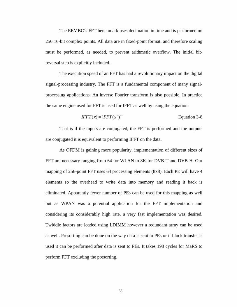
The EEMBC’s FFT benchmark uses decimation in time and is performed on
256 16-bit complex points. All data are in fixed-point format, and therefore scaling
must be performed, as needed, to prevent arithmetic overflow. The initial bit-
reversal step is explicitly included.
The execution speed of an FFT has had a revolutionary impact on the digital
signal-processing industry. The FFT is a fundamental component of many signal-
processing applications. An inverse Fourier transform is also possible. In practice
the same engine used for FFT is used for IFFT as well by using the equation:
** )]([)( xFFTxIFFT = Equation 3-8
That is if the inputs are conjugated, the FFT is performed and the outputs
are conjugated it is equivalent to performing IFFT on the data.
As OFDM is gaining more popularity, implementation of different sizes of
FFT are necessary ranging from 64 for WLAN to 8K for DVB-T and DVB-H. Our
mapping of 256-point FFT uses 64 processing elements (8x8). Each PE will have 4
elements so the overhead to write data into memory and reading it back is
eliminated. Apparently fewer number of PEs can be used for this mapping as well
but as WPAN was a potential application for the FFT implementation and
considering its considerably high rate, a very fast implementation was desired.
Twiddle factors are loaded using LDIMM however a redundant array can be used
as well. Presorting can be done on the way data is sent to PEs or if block transfer is
used it can be performed after data is sent to PEs. It takes 198 cycles for MaRS to
perform FFT excluding the presorting.

39
3.3.5 Viterbi decoder
The Viterbi Decoder benchmark exploits redundancy in a received data
stream to be able to recover the originally transmitted data. The benchmark
provides an indication of the potential performance of a microprocessor to be able
to process a forward error corrected (FEC) stream using the Viterbi algorithm.
A communication channel that is corrupted by noise typically uses FEC to
maintain transmission quality and efficiency. One such FEC mechanism is the use
of Convolutional encoding at the transmitter and the use of Viterbi decoding at the
receiver. The Viterbi decode process is an asymptotically optimum approach to the
decoding of Convolutional codes in a memory-less noise environment. Viterbi
decoding and the used terminology for that such as soft decoding will be elaborated
in details in following chapters. The trellis describes the state diagram of the
convolutional encoder as it evolves through time.
The benchmark implements a soft decision Viterbi decoder. The input is a
packet of 344 6-bit values each of which represents a pair of encoded bits. The 3-bit
value of each bit represents a soft decision value in the range 0 to 7. The value 0
indicates a strong indication that a 1 has been received while a value 7 indicates a
strong indication that a 0 has been received. The generator polynomials used for the
Convolutional encode process are:
1 + x + x3 + x5
1 + x2 + x3 + x4 + x5
Viterbi decoding is a computationally expensive process. The benchmark
explores the target CPU’s ability to perform loops, bit-wise operations, look-up

40
tables, comparisons and basic arithmetic operations. An approach similar to the one
used in the WLAN decoding implementation is used for GSM decoding i.e. a single
PE is dedicated to each state computation i.e. 32 PEs. The branch metric update is
broken into horizontal and vertical communications and needs 4 cycles. 1 cycle is
consumed performing ACS operation and 1 cycle for handling ACS bit. Trace-back
latency is hidden to a good extent and the overhead of sending trace-back bits to the
dedicated PE is minor.
3.3.6 EEMBC Telecomm suite results
MaRS is targeting wireless communication and DSP algorithm. Specifically
the emphasis has been on OFDM transceivers as it has been to be technology of
choice for beyond 3G. FFT and autocorrelation are widely used in OFDM receivers
and Viterbi decoder is seen in almost any wireless standard. The EEMBC
benchmark study illustrates capability of MaRS dealing with applications in the
area of interest.

41
Chapter 4 IEEE 802.11a PHY Algorithms
IEEE 802.11a PHY Algorithms
IEEE 802.11a is the second generation of wireless LAN standards
delivering higher rates up to five times more than IEEE 802.11b (54 Mbps vs. 11
Mbps). Moreover, IEEE 802.11a uses UNII 5 GHz frequency band which has more
bandwidth and less traffic compared to ISM 2.4 GHz. There are already a lot of
devices working at ISM band such as home RF, microwave oven, bluetooth and etc.
All these make IEEE 802.11a the wireless LAN standard choice of future.
4.1 IEEE 802.11a system overview and background
IEEE 802.11a uses Orthogonal Frequency Division Multiplexing (OFDM),
which turns out to perform very well in dispersive channels like wireless indoor
channel in addition to its bandwidth efficiency. A major advantage of OFDM is its
capability to perform in un-equalized multipath channels. OFDM transmits data on
parallel subcarriers, so the frequency selective fading channel is converted to flat
fading for each subcarrier. Therefore a one-tap frequency domain equalizer can be
used. ISI (Inter Symbol Interference) can be completely eliminated in OFDM by
inserting a Guard Interval (GI) between two consecutive symbols if the GI duration
is longer than channel RMS propagation delay. Though it seems power efficient

42
not to send anything in this guard interval, but in order to remove ICI (Inter Carrier
Interference) and maintain orthogonality, a part of the symbol is repeated in GI,
which is called cyclic prefix. This makes transmitting data in highly frequency
selective channels possible with cheap receivers. In addition to removing ICI, there
are a lot of synchronization algorithms that utilize use the redundancy of cyclic
prefix
The main drawback of OFDM is its sensitivity to frequency offset and its
vulnerability to non-synchronization; hence, synchronization algorithms are crucial
to the receiver performance.
In this research, synchronization algorithms for OFDM frame detection,
coarse and fine timing acquisition, coarse and fine carrier frequency offset
acquisition and correction and tracking algorithms are studied. A set of
implementation friendly algorithms are adopted and some of the algorithms are
modified or simplified to sub-optimal algorithms with minor performance
degradation. It should also be noted that HIPERLAN/2 and IEEE 802.11g OFDM
part are very similar to IEEE 802.11a, so most of the algorithms can be used for
those standards as well. Same algorithms can also be applied to IEEE 802.11n and
IEEE 802.16 standards.
The IEEE 802.11a physical layer uses coded OFDM with different
constellations and coding rates to provide different transmit rates from 6 Mbps to
54 Mbps where the maximum mandatory rate is 24 Mbps. The baseband signal is
constructed using 64-point IFFT in which 48 sub-carriers are data, 4 sub-carriers
are pilots and the remaining 12 sub-carriers are null to facilitate filters

43
implementation. In practice the signal is over-sampled before sending it to digital to
analog converter as it eliminates the need to compensate for the combined
frequency response of zero order hold and image rejection filter in DAC. Guard
interval makes design and computation of the image rejection ratio a lot easier.
Cyclic prefix is used in a guard interval of 1/4 (16 samples), which adds up
to 80 samples. With the sampling rate to be 20 MHz, each OFDM symbol’s
duration is 4µsec. Figure 4-1 shows block diagram of IEEE 802.11a PHY
transmitter.
Framing,Zero-Padding
Piolts Insertion,Subcarrier Mapping
Long and ShortTraining Sequences
and Signal Field
Scrambling,Conv olutional
Coding,Interleav ing,
QAM Mapping
Cy clic Pref ix,Windowing
Serial to ParallelFFT
Parallel to Serial
DAC,Analog Front End
and Antenna
Figure 4-1 – IEEE 802.11a Transmitter
MAC protocol data units (MPDU) are sent to physical layer along with the
burst profile information. The data may need to be padded to fit in integer number
of OFDM symbols.
Because of the burst nature of traffic in WLAN application, training
sequences are used for frequency and timing synchronization, channel estimation
and equalization. An 802.11a PHY frame is shown in Figure 4-2. Training
sequences consist of 10 short training sequences (16 samples each) and 2 long
sequences (64 sample each) and are pre-pended to each frame. The Signal field in
the frame contains data about rate, which implies constellation and code rate) and
number of octets (octet=8bits) in each packet. Signal field is coded with rate 1/2
and BPSK constellation is used which is the most robust transmission scheme.
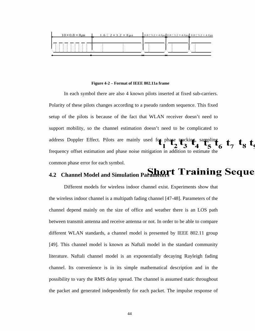
44
sµ88.010 =× sµ82.326.1 =×+ sµ0.42.38.0 =+ sµ0.42.38.0 =+ sµ0.42.38.0 =+
Figure 4-2 – Format of IEEE 802.11a frame
In each symbol there are also 4 known pilots inserted at fixed sub-carriers.
Polarity of these pilots changes according to a pseudo random sequence. This fixed
setup of the pilots is because of the fact that WLAN receiver doesn’t need to
support mobility, so the channel estimation doesn’t need to be complicated to
address Doppler Effect. Pilots are mainly used for phase tracking, sampling
frequency offset estimation and phase noise mitigation in addition to estimate the
common phase error for each symbol.
4.2 Channel Model and Simulation Parameters
Different models for wireless indoor channel exist. Experiments show that
the wireless indoor channel is a multipath fading channel [47-48]. Parameters of the
channel depend mainly on the size of office and weather there is an LOS path
between transmit antenna and receive antenna or not. In order to be able to compare
different WLAN standards, a channel model is presented by IEEE 802.11 group
[49]. This channel model is known as Naftali model in the standard community
literature. Naftali channel model is an exponentially decaying Rayleigh fading
channel. Its convenience is in its simple mathematical description and in the
possibility to vary the RMS delay spread. The channel is assumed static throughout
the packet and generated independently for each packet. The impulse response of

45
the channel is composed of complex samples with random uniformly distributed
phase and Rayleigh distributed magnitude with average power decaying
exponentially. The channel model can be formulated as the following equation
where hi is each tap coefficient which is a complex random variable that the real
and imaginary parts are Gaussian. It can be shown that the amplitude of such a
random variable has Rayleigh distribution and the phase has uniform distribution.
One should also notice the exponential decay of the taps with time.
RMSs
RMSs
TkT
TkTk
kki
e
e
jNNh
/20
/20
2
2212
21
1
1-4 Equation
),0(),0(
−
−
−=
=
+=
σσσ
σσ
where )21
,0( 2kN σ is a zero-mean Gaussian random variable with
variance 2
21
kσ , and RMSs TkTe /20 1 −−=σ is chosen so that the condition 12 =∑ kσ is
satisfied to ensure same average received power.
It is also assumed that the sampling time Ts in the simulation is shorter than
a symbol time by at least a factor of four (typically in simulations it is a sub-
multiple of the symbol duration). The number of samples to be taken in the impulse
response should ensure sufficient decay of the impulse response tail, e.g.
kmax=10TRMS/Ts. In our channel model, TRMS equal to 25 nsec is used. Other non-
ideal scenarios and transmitter’s front-end impairments are modeled in the channel
as well. Carrier Frequency Offset (CFO), power amplifier clipping because of high
Peak to Average Power Ratio (PAPR) of OFDM signal, fractional timing offset and
oscillator phase noise are phenomena to be modeled in the channel. It should be

46
noted that integer frequency offset is not a problem as the maximum allowed CFO
is about 200 KHz and the CFO estimation algorithm range is around 625 KHz.
A random delay is then added to test the frame detection algorithm and
timing synchronization functions. Finally base-band Gaussian noise is added to the
signal. In our simulations, fractional timing offset and phase noise are not modeled
for simplicity; however, the residual CFO error can be considered as phase noise
and the CFO tracking algorithm used is a phase noise suppressing one. Best way to
deal with fractional timing error is to send a feedback signal to the analog front-end.
In baseband processing, interpolation can be used to compensate for error which is
not as efficient of analog methods and the frequency domain equalizer also corrects
the effect of fractional timing error.
There may also be other concerns or an actual product that would depend on
the analog front end and would appear in the integration phase. For instance, if the
analog transceiver has IQ-mismatch the constellation would be distorted; or if
cheap crystal is used in the transceiver sampling frequency offset may exist which
will lead to higher error vector magnitude (EVM).
4.3 Receiver Algorithms
Receiver algorithms are usually choice of the designers as long as they can
meet some minimum performance requirements. Receiver algorithms determine the
complexity of design and eventually the final price; however performance of a
receiver relies on the algorithms as well.
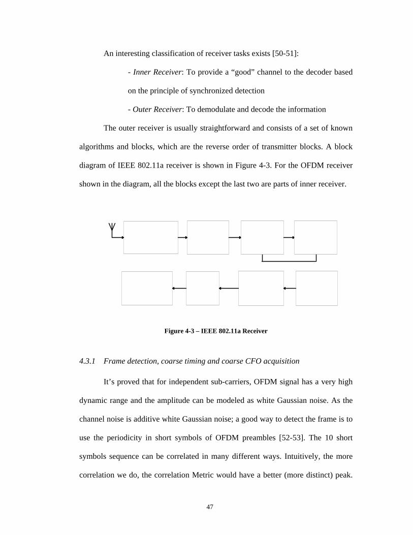
47
An interesting classification of receiver tasks exists [50-51]:
- Inner Receiver: To provide a “good” channel to the decoder based
on the principle of synchronized detection
- Outer Receiver: To demodulate and decode the information
The outer receiver is usually straightforward and consists of a set of known
algorithms and blocks, which are the reverse order of transmitter blocks. A block
diagram of IEEE 802.11a receiver is shown in Figure 4-3. For the OFDM receiver
shown in the diagram, all the blocks except the last two are parts of inner receiver.
Figure 4-3 – IEEE 802.11a Receiver
4.3.1 Frame detection, coarse timing and coarse CFO acquisition
It’s proved that for independent sub-carriers, OFDM signal has a very high
dynamic range and the amplitude can be modeled as white Gaussian noise. As the
channel noise is additive white Gaussian noise; a good way to detect the frame is to
use the periodicity in short symbols of OFDM preambles [52-53]. The 10 short
symbols sequence can be correlated in many different ways. Intuitively, the more
correlation we do, the correlation Metric would have a better (more distinct) peak.
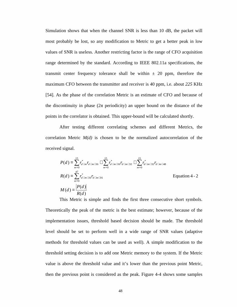
48
Simulation shows that when the channel SNR is less than 10 dB, the packet will
most probably be lost, so any modification to Metric to get a better peak in low
values of SNR is useless. Another restricting factor is the range of CFO acquisition
range determined by the standard. According to IEEE 802.11a specifications, the
transmit center frequency tolerance shall be within ± 20 ppm, therefore the
maximum CFO between the transmitter and receiver is 40 ppm, i.e. about 225 KHz
[54]. As the phase of the correlation Metric is an estimate of CFO and because of
the discontinuity in phase (2π periodicity) an upper bound on the distance of the
points in the correlator is obtained. This upper-bound will be calculated shortly.
After testing different correlating schemes and different Metrics, the
correlation Metric M(d) is chosen to be the normalized autocorrelation of the
received signal.
)(
)()(
2-4 Equation)(
)(
47
016
*16
15
048
*32
15
032
*16
15
016
*
dR
dPdM
rrdR
rrrrrrdP
mmdmd
mmdmd
mmdmd
mmdmd
=
=
++=
∑
∑∑∑
=++++
=++++
=++++
=+++
This Metric is simple and finds the first three consecutive short symbols.
Theoretically the peak of the metric is the best estimate; however, because of the
implementation issues, threshold based decision should be made. The threshold
level should be set to perform well in a wide range of SNR values (adaptive
methods for threshold values can be used as well). A simple modification to the
threshold setting decision is to add one Metric memory to the system. If the Metric
value is above the threshold value and it’s lower than the previous point Metric,
then the previous point is considered as the peak. Figure 4-4 shows some samples
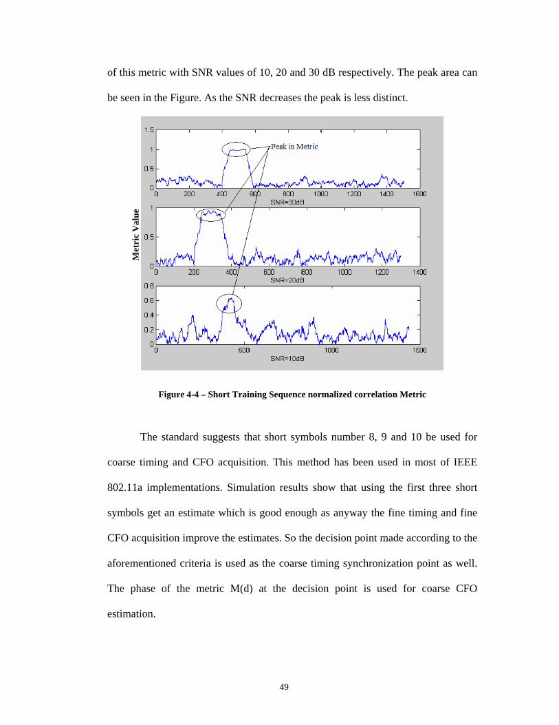
49
of this metric with SNR values of 10, 20 and 30 dB respectively. The peak area can
be seen in the Figure. As the SNR decreases the peak is less distinct.
Figure 4-4 – Short Training Sequence normalized correlation Metric
The standard suggests that short symbols number 8, 9 and 10 be used for
coarse timing and CFO acquisition. This method has been used in most of IEEE
802.11a implementations. Simulation results show that using the first three short
symbols get an estimate which is good enough as anyway the fine timing and fine
CFO acquisition improve the estimates. So the decision point made according to the
aforementioned criteria is used as the coarse timing synchronization point as well.
The phase of the metric M(d) at the decision point is used for coarse CFO
estimation.
Met
ric V
alue
50
The CFO is related to θ, i.e. M(d) angle, according to:
STN
CFOπ
θ2
= Equation 4-3
where Ns is the number of points in a short symbol, i.e. 16, T is elementary
period of signal which is duration of each sample i.e. 50 nsec. Deriving the
relationship between CFO and θ is straightforward as the CFO term factors out of
the correlation Metric summation. Acquisition range of this implementation of CFO
can be found by substituting θ with π.
KHzTNTN
CFOsS
6252
1|
2max === =πθπθ Equation 4-4
This is beyond what is required by the standard. An important point for
implementation is that calculation of metric M(d) can be done recursively re-using
most of the computations already done using a sliding window technique. So for
computation of a new metric, the new contributor to summation is added and the
oldest contributor is subtracted and the all mid-points do not need to be computed
again.
4.3.2 Fine Timing Synchronization, Fine CFO and Channel Estimation
For fine timing synchronization, long training sequences, which consists of
two identical symbols prepended by guard interval is used. The long symbol is
designed in such a way that its autocorrelation almost looks like the delta function.
Auto correlation can be used to utilize the periodicity in the long symbol to perform
fine timing synchronization the same way we used for coarse timing
synchronization. Another possible approach is based on the fact that the actual long
symbol is known at the receiver. Therefore cross correlation of actual long symbol
51
with the received symbol should result in two peaks, which the first peak is
beginning of the long symbols and the fine timing synchronization decision point.
Using this algorithm is a trade-off between computation overhead and performance.
This Metric summation can’t be implemented using increment-decrement sliding
window method and doesn’t give the fine CFO estimate so another Metric should
be computed for CFO as well, but the peaks produced by this algorithm are quite
distinct. The reason is that autocorrelation for the former Metric is continuous so
there is a higher probability that noise can displace the peak however the latter one
just results in a single peak. The latter algorithm is used in the simulations. This
metric can be formulated as:
∑=
+=63
0
*)(m
mmd lrdP
∑=
++=63
0
*)(m
mdmd rrdR Equation 4-4
)()(
)(dR
dPdM =
where lm is the actual value of long training sequence kept locally in the
receiver and r is the received signal. The overhead can be negligible for DSP
processors with arrays including tens of multipliers; however, if the overhead seems
too much for a specific architecture, the regular autocorrelation metric can be used
sacrificing some performance. Figure 4-5 shows the metric generated using known
long training sequence correlation with received signal in SNR values of 10, 20 and
30 dB respectively. Two conspicuous peaks can be noticed in the diagram. The
same combination of threshold based and single-entry peak finding algorithm is

52
used in fine timing as well. Note that smaller threshold values are preferred as early
detected frames can be corrected because of the cyclic prefix (if the signal is
circularly rotated in time domain, in the frequency domain it is multiplied by a
phasor), whereas the late frame detection will result in loss of data.
Once the fine timing decision is made, the autocorrelation between first and
second long symbol is calculated. This correlation Metric can be formulated as:
pointtimingfine
63
064
* |)( ==
+++∑= dm
mdmd rrdP Equation 4-5
This correlation should be calculated only once when the fine timing is
found from correlation with actual long training sequence. The phase of this metric
gives a fine estimate of CFO. The acquisition range for this algorithm is found to be
156.25 KHz using the same formula as coarse CFO with N=64. The residual
frequency error after coarse CFO correction is usually much less than this amount
so it’s well within the range; however, it implies the necessity for a coarse CFO
estimator using short training sequence.
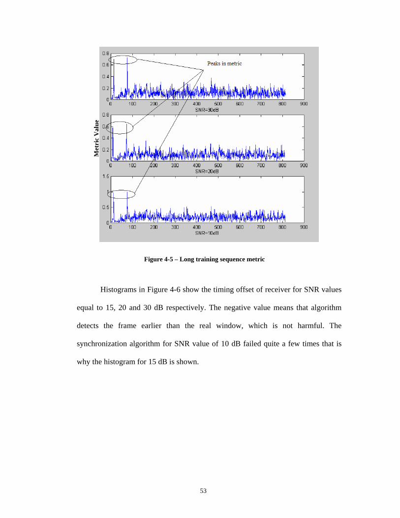
53
Figure 4-5 – Long training sequence metric
Histograms in Figure 4-6 show the timing offset of receiver for SNR values
equal to 15, 20 and 30 dB respectively. The negative value means that algorithm
detects the frame earlier than the real window, which is not harmful. The
synchronization algorithm for SNR value of 10 dB failed quite a few times that is
why the histogram for 15 dB is shown.
Met
ric V
alue
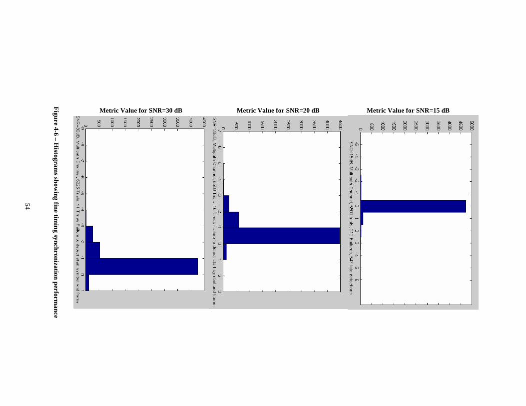
54
Figure 4-6 – H
istograms show
ing fine timing synchronization perform
ance
Metric Value for SNR=15 dB Metric Value for SNR=20 dB Metric Value for SNR=30 dB

55
Next step is to correct the CFO, which is multiplication by a phasor.
Simulations are also made to check the performance of our CFO acquisition
algorithms. Same system set up as previous one is used with CFO of 200 KHz.
Figure 4-7 diagrams show performance of the CFO acquisition algorithm. The
diagram shows the residual CFO after the fine CFO estimation and correction in a
realistic channel scenario.
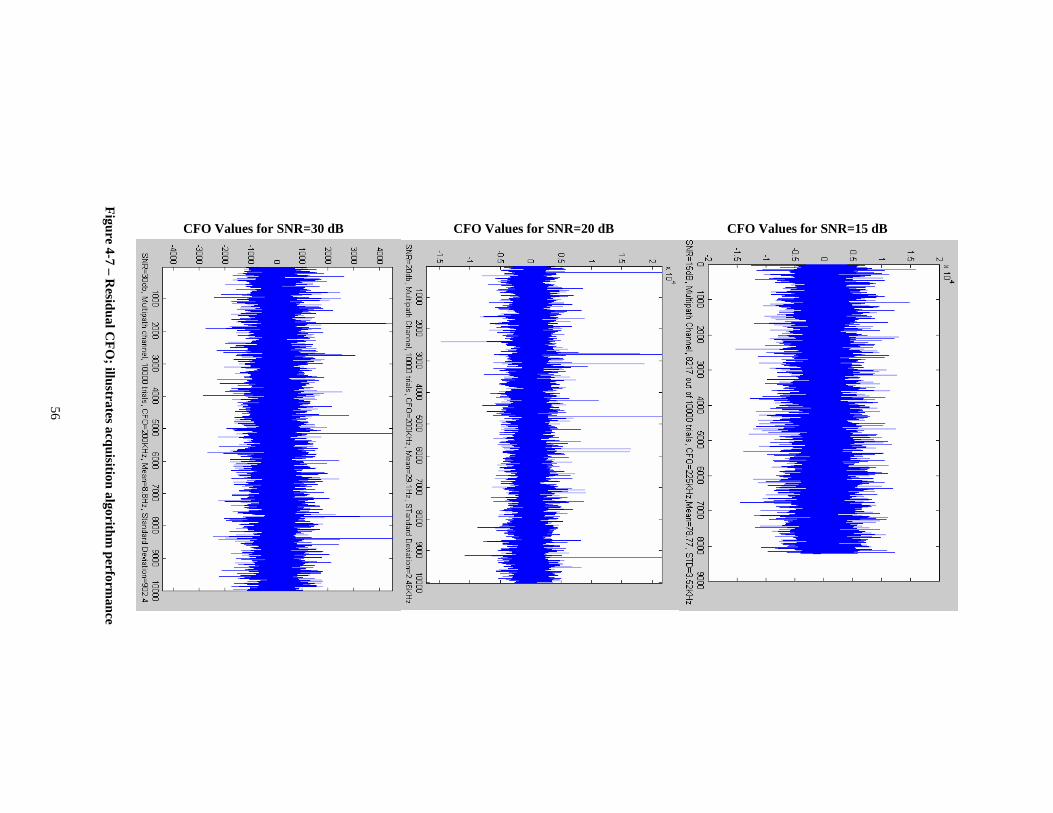
56
Figure 4-7 – R
esidual CF
O; illustrates acquisition algorithm
performance
CFO Values for SNR=30 dB CFO Values for SNR=20 dB CFO Values for SNR=15 dB

57
Consequently the FFT of the received long signals is computed for both
long symbols and the average is computed. Averaging mitigates the contribution of
the noise in the preambles. Dividing the averaged received long signal by the
known values, gives the channel impulse response (DFT of the channel). These
values will be used for frequency domain one tap equalization. Figure 4-8 shows
the DFT of CIR and the estimated CIR in SNR=20dB. This concludes algorithms
for inner receiver of IEEE 802.11a standard receiver. Noise effect on channel is
considerable because only two long symbols exist and not enough averaging is done
to mitigate noise effect.
Figure 4-8 – Channel estimation performance in SNR=20dB
4.3.3 Tracking Algorithms
For CFO tracking, either pilots or the cyclic prefix should be used. The fact
that cyclic prefix is exactly similar to the last part of OFDM symbol can be used for
CFO tracking using the same correlation metric we have used throughout the
system design and simulation. Cyclic prefix method is used extensively in
Nor
mal
ized
Cha
nnel
Res
pons
e
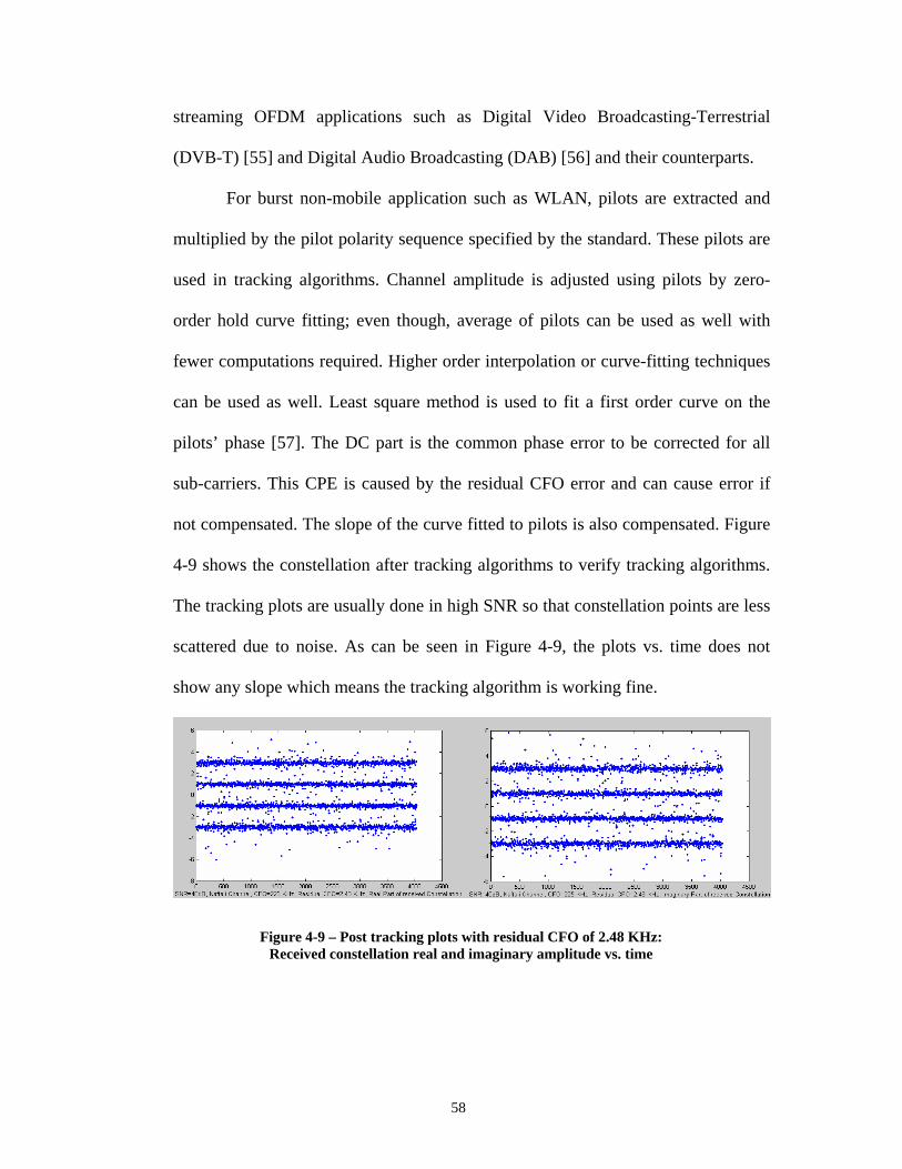
58
streaming OFDM applications such as Digital Video Broadcasting-Terrestrial
(DVB-T) [55] and Digital Audio Broadcasting (DAB) [56] and their counterparts.
For burst non-mobile application such as WLAN, pilots are extracted and
multiplied by the pilot polarity sequence specified by the standard. These pilots are
used in tracking algorithms. Channel amplitude is adjusted using pilots by zero-
order hold curve fitting; even though, average of pilots can be used as well with
fewer computations required. Higher order interpolation or curve-fitting techniques
can be used as well. Least square method is used to fit a first order curve on the
pilots’ phase [57]. The DC part is the common phase error to be corrected for all
sub-carriers. This CPE is caused by the residual CFO error and can cause error if
not compensated. The slope of the curve fitted to pilots is also compensated. Figure
4-9 shows the constellation after tracking algorithms to verify tracking algorithms.
The tracking plots are usually done in high SNR so that constellation points are less
scattered due to noise. As can be seen in Figure 4-9, the plots vs. time does not
show any slope which means the tracking algorithm is working fine.
Figure 4-9 – Post tracking plots with residual CFO of 2.48 KHz: Received constellation real and imaginary amplitude vs. time
59
After tracking steps are done, other parts of outer receiver can be performed.
These parts are basically the reverse of what has been done in the transmitter as is
outlined in the following section.
4.3.4 Outer receiver
The sensitivity of a WLAN receiver is based on the link budget analysis and
is related to SNR that gives a certain amount of probability of error and is fixed in
standard, noise figure and implementation cost of the receiver. Noise figure is an
issue in the RF and analog front-end whereas the implementation cost is related to
the algorithm used. Therefore any algorithm leading to a lower implementation cost
increases the sensitivity of the receiver and adds to the value of the product.
Using soft decision decoding is a known technique to boost the performance
of Viterbi decoders by keeping the bit-metrics instead of making 0/1 decisions. Soft
decision decoding is much more complicated but advances in the VLSI technology
has facilitated realizing very fast parallel soft decision Viterbi decoders.
Performance of Soft Viterbi decoder can be improved even more for OFDM
systems utilizing channel state information (CSI). This concept is elaborated in
details in what follows.
Let’s assume that t[i] is the modulated sub-carrier, which is a point from the
constellation. At the receiving end, after the inner receiver synchronization part and
OFDM demodulator the r[i] corresponding to t[i] would be:
][][].[][ initihir += Equation 4-6
where h is the channel response at i th sub-carrier and n is the channel noise.
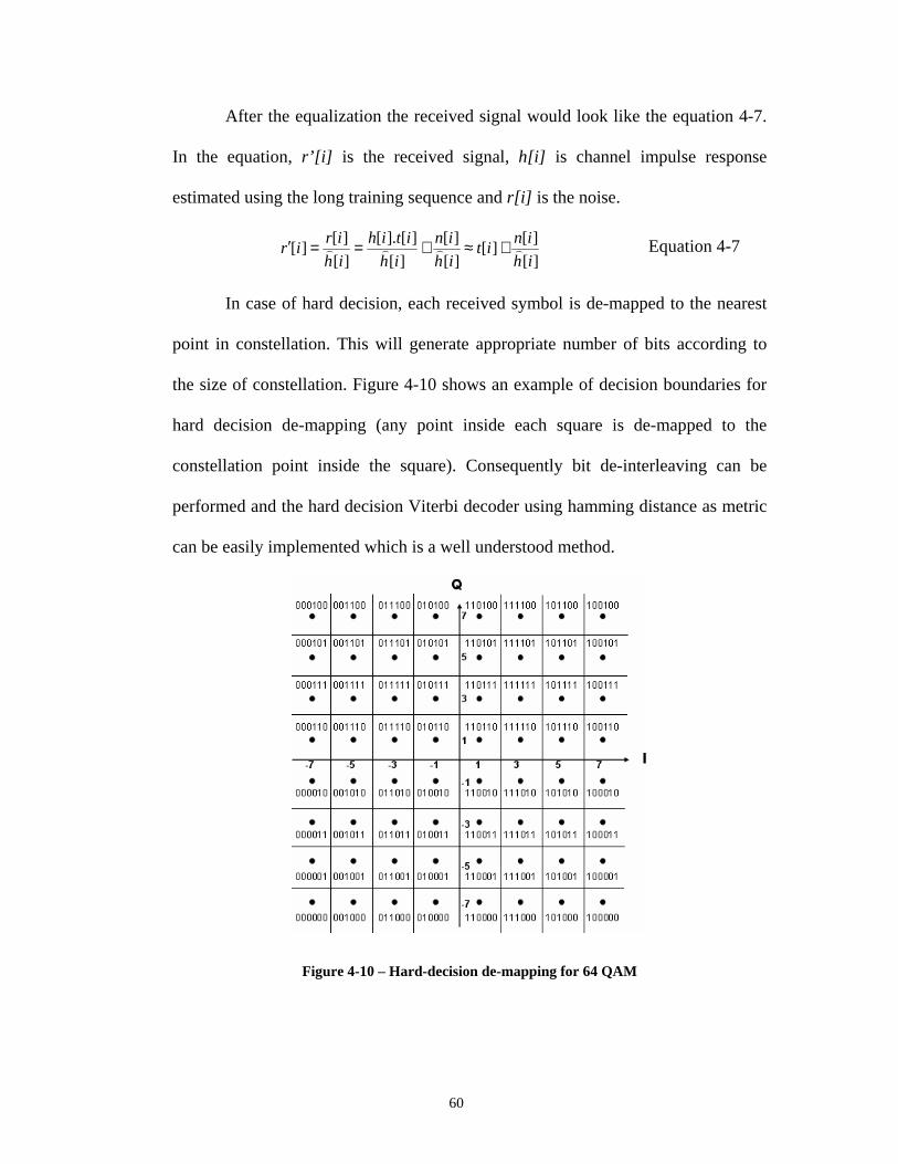
60
After the equalization the received signal would look like the equation 4-7.
In the equation, r’[i] is the received signal, h[i] is channel impulse response
estimated using the long training sequence and r[i] is the noise.
][
][][
][
][
][
][].[
][
][][
ih
init
ih
in
ih
itih
ih
irir )))) +≈+==′ Equation 4-7
In case of hard decision, each received symbol is de-mapped to the nearest
point in constellation. This will generate appropriate number of bits according to
the size of constellation. Figure 4-10 shows an example of decision boundaries for
hard decision de-mapping (any point inside each square is de-mapped to the
constellation point inside the square). Consequently bit de-interleaving can be
performed and the hard decision Viterbi decoder using hamming distance as metric
can be easily implemented which is a well understood method.
Figure 4-10 – Hard-decision de-mapping for 64 QAM

61
The problem with hard decision is that it does not differentiate between a
received point, which is exactly on the constellation and a point, which is on the
boundary of two or even four adjacent symbols. However, we have more certainty
in the former case than we have in the latter one about the decision we are making.
Soft-decision decoding is a way to quantize this degree of certainty and make use of
it. As there is a de-interleaver after de-mapping, maximum likelihood decoding of
multi-level Bit Interleaved Coded Modulation (BICM) signals requires joint
demodulation and decoding which is very complicated to implement, therefore
using the log likelihood ratio method like Zehavi’s method to compute sub-optimal
simplified bit metrics for BICM is considered [57-59]. For each in-phase and
quadrature bits, two metrics need to be computed. For each bit bk corresponding to
values 0, 1 the constellation is split into two partitions of complex plane namely S0k
and S1k where the former means the metric is closer to 0 and the latter means that
the metric is closer to 1. This partitioning is performed by looking at a certain bit in
the constellation. All the points with that bit set to 0, fall in to S0k partition and all
the points with that bit set to 1, fall in to S1k partition.
The decision boundaries for 64-QAM constellation used in IEEE 802.11a
standard are shown in Figures 4-11a-f.
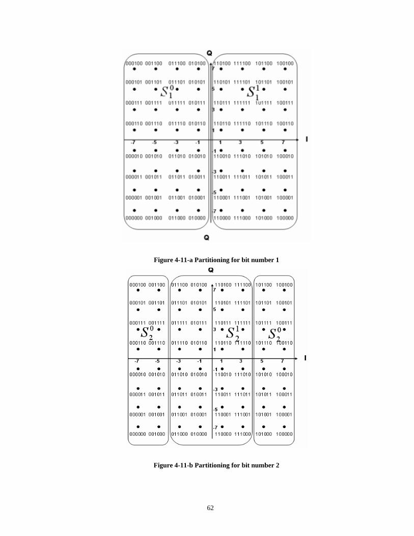
62
Figure 4-11-a Partitioning for bit number 1
Figure 4-11-b Partitioning for bit number 2
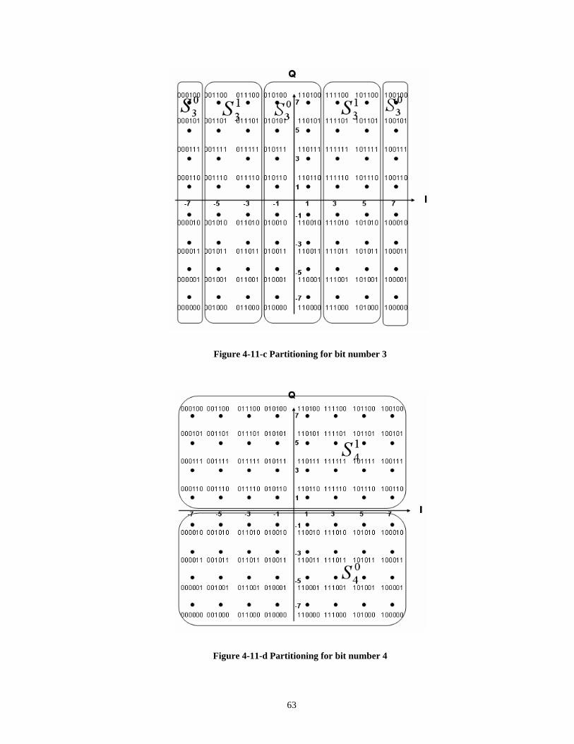
63
Figure 4-11-c Partitioning for bit number 3
Figure 4-11-d Partitioning for bit number 4

64
Figure 4-11-e Partitioning for bit number 5
Figure 4-11-f Partitioning for bit number 6
Figure 4-11a-f – Partitions of constellation to subsets ‘0’ and ‘1’ for 64QAM

65
Bit metric computation for smaller constellations is simpler than 64 QAM
case. The constellation space is partitioned to n regions where n is the number of
bits/symbol.
There are some issues regarding the number of bits required to represent bit
metrics. Simulations show that there is a saturation point in the performance vs.
precision plot for soft Viterbi decoder. It is demonstrated that there is no
considerable gain reached by using more than four bits. This also implies saturating
the metrics that are greater than the maximum metric presentable by dedicated
number of bits. From implementation point of view, using 4 bits makes
implementation of bit metric computation function easy using look up tables with
16 entries.
By looking at Equation 4-7 for received symbol, one can notice that
equalizer may cause some noise enhancements i.e. noise is multiplied by the inverse
of channel impulse response. For subcarriers that experience fading the inverse of
channel can be huge leading to considerable noise enhancement.
In order to cancel out the possible noise enhancements caused by the noise
term divided by channel estimates, bit metrics are normalized by the magnitude of
the corresponding equalizer tap. This is another step where the channel state
information is involved in decoding process. So the final bit metric can be
approximated by Equation 4-8.
][
][][][][Bit_Metric
2
2
ih
inihitih )
)
)+≈ Equation 4-8

66
Another advantage of this metric adjustment is that more weight is given to
sub-channels with more certainty i.e. larger][ ih)
. Once the bit metrics are computed,
de-interleaving is done. De-interleaving is reverse of the transmitter’s side
interleaver. In case de-puncturing is needed, bit metrics to both 0 and 1 is set to zero
to prevent the de-punctured bits from changing the state metric in traversing trellis.
Next block is a simple standard Viterbi algorithm. In hardware implementation
either trace-back or register exchange method can be used without any change in
performance. Another implementation point is depth of decoding. As a rule of
thumb depth of decoding is chosen to be 5 times constraint length which is 35 for
our case. Simulation results confirm that decoding depth of 35 is ok. However for
punctured code higher values of trace-back should be used. There is a trade-off
between the size of memory needed for trace-back data and the overhead associated
with the trace-back operation.
In order to compare the performance of hard decision and soft decision, an
IEEE 802.11a system is set up. Different rates are transmitted by the standard
utilizing different code rates and different constellations. Because of the application
of WLAN, which is in packet transmission and as the size of packet is limited; BER
is not a good criterion for performance analysis. A better measure is PER
(Packet/PPDU Error Rate). For this purpose, packets are sent along channel.
Multipath channel is generated for each packet separately and PER table versus
SNR is filled. The PER=0.08 is the point where soft decision and hard decision are
compared to determine the soft decision decoding gain. For brevity, only one
simulation per constellation is performed. Our simulations are done for rates 9
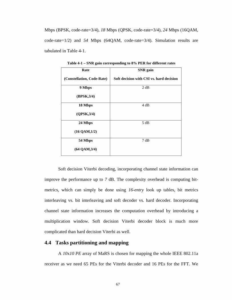
67
Mbps (BPSK, code-rate=3/4), 18 Mbps (QPSK, code-rate=3/4), 24 Mbps (16QAM,
code-rate=1/2) and 54 Mbps (64QAM, code-rate=3/4). Simulation results are
tabulated in Table 4-1.
Table 4-1 – SNR gain corresponding to 8% PER for different rates
Rate
(Constellation, Code-Rate)
SNR gain
Soft decision with CSI vs. hard decision
9 Mbps
(BPSK,3/4)
2 dB
18 Mbps
(QPSK,3/4)
4 dB
24 Mbps
(16 QAM,1/2)
5 dB
54 Mbps
(64 QAM,3/4)
7 dB
Soft decision Viterbi decoding, incorporating channel state information can
improve the performance up to 7 dB. The complexity overhead is computing bit-
metrics, which can simply be done using 16-entry look up tables, bit metrics
interleaving vs. bit interleaving and soft decoder vs. hard decoder. Incorporating
channel state information increases the computation overhead by introducing a
multiplication window. Soft decision Viterbi decoder block is much more
complicated than hard decision Viterbi as well.
4.4 Tasks partitioning and mapping
A 10x10 PE array of MaRS is chosen for mapping the whole IEEE 802.11a
receiver as we need 65 PEs for the Viterbi decoder and 16 PEs for the FFT. We
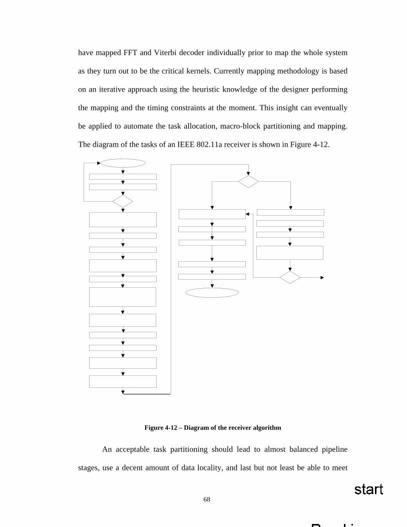
68
have mapped FFT and Viterbi decoder individually prior to map the whole system
as they turn out to be the critical kernels. Currently mapping methodology is based
on an iterative approach using the heuristic knowledge of the designer performing
the mapping and the timing constraints at the moment. This insight can eventually
be applied to automate the task allocation, macro-block partitioning and mapping.
The diagram of the tasks of an IEEE 802.11a receiver is shown in Figure 4-12.
Figure 4-12 – Diagram of the receiver algorithm
An acceptable task partitioning should lead to almost balanced pipeline
stages, use a decent amount of data locality, and last but not least be able to meet

69
the stringent timing requirement of a multi-rate standard such as IEEE 802.11a. An
example of task allocation and partitioning is shown in Figure 4-13.
Figure 4-13 – Tasks allocation on PEs
Notice that more than one task is sometimes mapped onto a PE. The total number of
macro-blocks is seven. Some of them such as scrambling and de-puncturing are
straightforward and only consist of a single PE, while the macro-block for the trellis
traversal of the Viterbi decoder consists of 64 PEs. Table 4-2 shows the mapping
statistics of different kernels for a 54Mbps receiver.
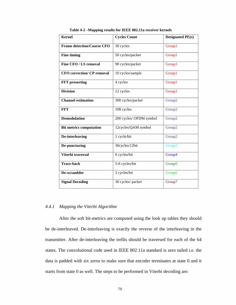
70
Table 4-2 –Mapping results for IEEE 802.11a receiver kernels
Kernel Cycles Count Designated PE(s)
Frame detection/Coarse CFO 30 cycles Group1
Fine timing 50 cycles/packet Group1
Fine CFO / LS removal 90 cycles/packet Group1
CFO correction/ CP removal 10 cycles/sample Group1
FFT presorting 4 cycles Group1
Division 12 cycles Group1
Channel estimation 300 cycles/packet Group2
FFT 108 cycles Group2
Demodulation 200 cycles/ OFDM symbol Group2
Bit metrics computation 12cycles/QAM symbol Group2
De-interleaving 1 cycle/bit Group2
De-puncturing 30cycles/12bit Group3
Viterbi traversal 6 cycles/bit Group4
Trace-back 5-6 cycles/bit Group5
De-scrambler 3 cycles/bit Group6
Signal Decoding 30 cycles/ packet Group7
4.4.1 Mapping the Viterbi Algorithm
After the soft bit-metrics are computed using the look up tables they should
be de-interleaved. De-interleaving is exactly the reverse of the interleaving in the
transmitter. After de-interleaving the trellis should be traversed for each of the 64
states. The convolutional code used in IEEE 802.11a standard is zero tailed i.e. the
data is padded with six zeros to make sure that encoder terminates at state 0 and it
starts from state 0 as well. The steps to be performed in Viterbi decoding are:

71
1. An Add-Compare-Select (ACS) operation should be performed on the
received bit-metrics. Each state has two predecessors and the code polynomials
define the output of the decoder for any input. Depending on the expected output,
the state metric is added/subtracted to/from the predecessors’ state metrics (Add),
then these two new metrics are compared (Compare) and the better metric is
selected (Select), hence ACS. In addition, a flag, to be used later in decoding, is set
or reset if the survivor comes from the upper source or lower source, respectively.
2. The updated state metrics are sent to the two possible successor states for
the next iteration. This is the state metric update phase of the decoder.
Each branch taken in any iteration needs to be recorded so that the original
data can be reconstructed from the path that is associated with the smallest state
metric after the trellis has converged. As a rule of thumb, the decoding depth (the
number of iterations before the trellis converges) is supposed to be five times more
than the constraint length, which is 30-35 for the case of 802.11a. This value should
be more punctured code to account for the stolen bits in the transmitter.
Decoding can be done in either register exchange method or trace-back
method. In trace-back, decoding is accomplished by storing all ACS flags in a
matrix of 64 by the number of iterations before trace-back is scheduled to be
performed. During trace-back, the state that winds up with the minimal state metric
is used as a starting point, and the matrix is traversed backwards, using the recorded
bits in each column to determine which row to check in the previous column. The
sequence of these bits (in reverse order) is the decoded data. The alternative method
is register exchange in which the ACS flag is the actual decoded bit (i.e. possible
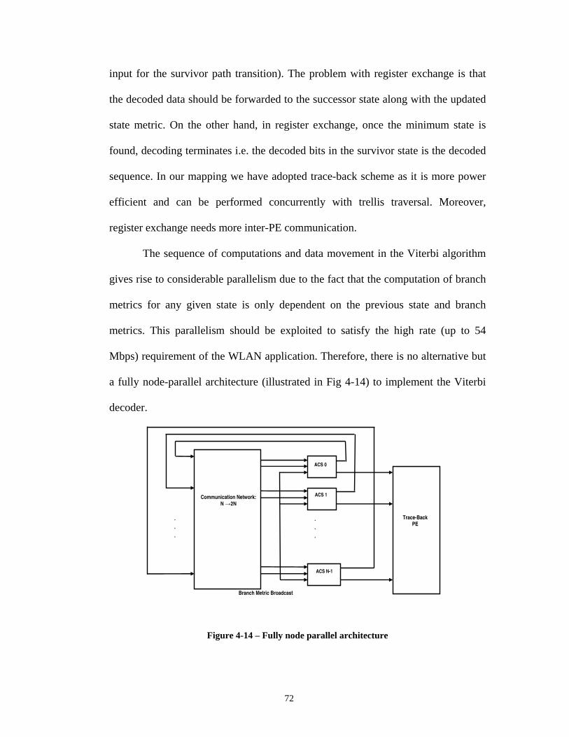
72
input for the survivor path transition). The problem with register exchange is that
the decoded data should be forwarded to the successor state along with the updated
state metric. On the other hand, in register exchange, once the minimum state is
found, decoding terminates i.e. the decoded bits in the survivor state is the decoded
sequence. In our mapping we have adopted trace-back scheme as it is more power
efficient and can be performed concurrently with trellis traversal. Moreover,
register exchange needs more inter-PE communication.
The sequence of computations and data movement in the Viterbi algorithm
gives rise to considerable parallelism due to the fact that the computation of branch
metrics for any given state is only dependent on the previous state and branch
metrics. This parallelism should be exploited to satisfy the high rate (up to 54
Mbps) requirement of the WLAN application. Therefore, there is no alternative but
a fully node-parallel architecture (illustrated in Fig 4-14) to implement the Viterbi
decoder.
Figure 4-14 – Fully node parallel architecture
Communication Network: N →2N
ACS 0
Trace-Back PE
ACS 1
Branch Metric Broadcast
.
.
.
.
.
.
ACS N-1

73
The large amount of communication required by the “state metric update”
phase of the Viterbi algorithm makes it a communication intensive application
besides computation intensive. In order to minimize the communication overhead,
the 64 nodes required for node-parallel Viterbi decoder are chosen to be in an 8 by
8 array of PEs. The communication pattern required by the “state metric update”
phase of the Viterbi algorithm is in a way that assuming the current state of the
encoder is an-1…a1a0, the next state will be either 1an-1…a1 or 0an-1…a1. This
interconnection network is well defined and is called shuffle-exchange network.
However, the shuffle network depends on size, i.e. circular shift depends on the size
of register. This makes the shuffle network an inappropriate choice when flexibility
is a design criterion; however, this communication pattern significantly benefits
from the distributed shared register file introduced in MaRS. Using the mesh
network for communicating with adjacent neighbors and the shared register file for
distant communications, MaRS can perform the communication for the state metric
update in 4 cycles. This will be elaborated soon in details using step by step pseudo-
code.
The trellis traversal procedure is on the critical path of the Viterbi decoder.
In order to achieve a good cycles/bit for the CC(2,1,7) soft decision Viterbi decoder
the PE’s ALU is enhanced with an ACS unit capable of performing half-trellis
butterfly in one cycle. The ACS unit consists of two accumulators which will be
loaded with the current state metric. The branch metrics are also available in the PE
prior to ACS. Each accumulator will have to simply add/subtract operations on two.
74
The instruction format of ACS is given below.
(R0, ACS-Flag)=ACS (SM0, SM1, BM)
The ACS unit as described above has the chance of metric overflow, so after
each iteration the metrics should be subtracted by a constant value to avoid
overflow. There are some methods in the literature that are used in optimized ASIC
Viterbi decoder designs that use modular operation. One of such methods is to
replace the ACS unit with ASCS (Add, Subtract, Compare, Subtract) published by
Ungerboeck [61]. This datapath is based on 2’s complement format and avoids
metric’s overflow. The first version of ACS module designed for MaRS does not
use that technique but that design is noteworthy for future enhancements.
Moreover, to manipulate the trace-back flag, there is an ‘insert’ bit
instruction added to MaRS ISA. This instruction sets an arbitrary bit in the register
specified in the instruction if the specified flag is set. Correspondingly there is also
a ‘read’ bit instruction as well which will be used in trace-back phase. Finally, the
register file is word addressable and the instructions can use one full register or two
half registers as their operand.
The trellis traversal part of the Viterbi algorithm is coded and mapped onto
MaRS architecture. It takes MaRS 6 cycles to perform this part of the algorithm.
The first four cycles are spent performing state metric update and cycles 5 and 6 are
dedicated to ACS and ACS-flag handling. The pseudo-code for this algorithm is as
follows.
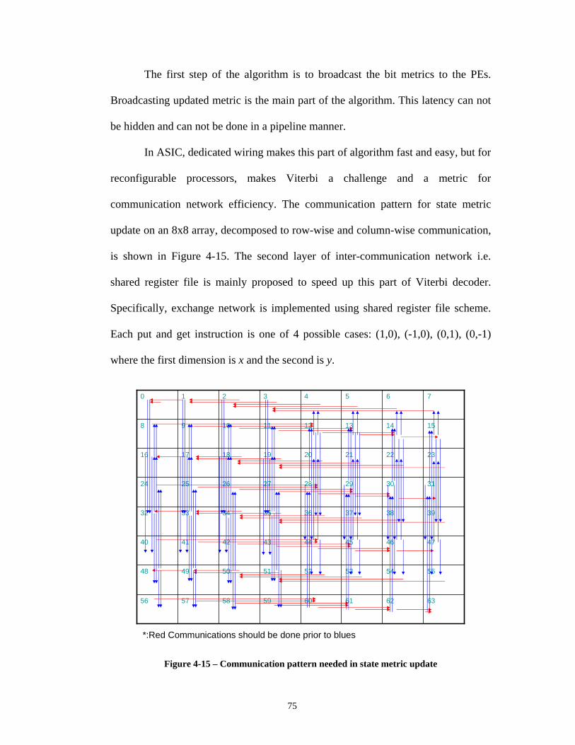
75
The first step of the algorithm is to broadcast the bit metrics to the PEs.
Broadcasting updated metric is the main part of the algorithm. This latency can not
be hidden and can not be done in a pipeline manner.
In ASIC, dedicated wiring makes this part of algorithm fast and easy, but for
reconfigurable processors, makes Viterbi a challenge and a metric for
communication network efficiency. The communication pattern for state metric
update on an 8x8 array, decomposed to row-wise and column-wise communication,
is shown in Figure 4-15. The second layer of inter-communication network i.e.
shared register file is mainly proposed to speed up this part of Viterbi decoder.
Specifically, exchange network is implemented using shared register file scheme.
Each put and get instruction is one of 4 possible cases: (1,0), (-1,0), (0,1), (0,-1)
where the first dimension is x and the second is y.
6362616059585756
5554535251504948
4746454443424140
3938373635343332
3130292827262524
2322212019181716
15141312111098
76543210
*:Red Communications should be done prior to blues
Figure 4-15 – Communication pattern needed in state metric update

76
Assuming that the ACS operation is performed and the new metric is
computed at each state (for a node parallel Viterbi decoder). Table 4-4 shows the
number of each state metric in eight-by-eight array of PEs. The rows and columns
of the table correspond to row and columns of the array.
Table 4-3 –Allocation of trellis states in each PE
0
1 2 3 4 5 6 7
8
9 10 11 12 13 14 15
16
17 18 19 20 21 22 23
24
25 26 27 28 29 30 31
32
33 34 35 36 37 38 39
40
41 42 43 44 45 46 47
48
49 50 51 52 53 54 55
56
57 58 59 60 61 62 63

77
Instructions in each PE in cycle 1 are illustrated in Table 4-5. In the first
cycle, PEs use the dedicated communication network to communicate with
neighboring PEs. All of the PEs use either PUT or GET instructions. The R register
can be two half registers as well.
Table 4-4 –Instructions in the first cycle
Get R,1,0
Put R,-1,0
Put R,1,0
Get R,-1,0
Get R,1,0
Put R,-1,0
Put R,1,0
Get R,-1,0
Get R,1,0
Put R,-1,0
Put R,1,0
Get R,-1,0
Get R,1,0
Put R,-1,0
Put R,1,0
Get R,-1,0
Get R,1,0 Put R,-1,0
Put R,1,0
Get R,-1,0 Get R,1,0 Put R,-1,0
Put R,1,0
Get R,-1,0
Get R,1,0
Put R,-1,0
Put R,1,0
Get R,-1,0
Get R,1,0
Put R,-1,0
Put R,1,0
Get R,-1,0
Get R,1,0
Put R,-1,0
Put R,1,0
Get R,-1,0
Get R,1,0
Put R,-1,0
Put R,1,0
Get R,-1,0
Get R,1,0
Put R,-1,0
Put R,1,0
Get R,-1,0
Get R,1,0
Put R,-1,0
Put R,1,0
Get R,-1,0
Get R,1,0
Put R,-1,0
Put R,1,0
Get R,-1,0
Get R,1,0
Put R,-1,0
Put R,1,0
Get R,-1,0
Get R,1,0
Put R,-1,0
Put R,1,0
Get R,-1,0
Get R,1,0
Put R,-1,0
Put R,1,0
Get R,-1,0
Table 4-6 shows the location of state metric after first cycle. It should be
noted that the first two cycles achieve the communication shown with red arrows in
Figure 4-16 and the cycles three and four perform the blue arrows communications.
Table 4-5 –State metrics distribution after first cycle
0,1
1 2 3,2 4,5 5 6 7,6
8,9
9 10 11,10 12,13 13 14 15,14
16,17
17 18 19,18 20,21 21 22 23,22
24,25
25 26 27,26 28,29 29 30 30,31
32,33
33 34 35,34 36,37 37 38 39,38
40,41
41 42 43,42 44,45 45 46 47,46
48,49
49 50 51,50 52,53 53 54 55,54
56,57 57
58 59,58 60,61 61 62 63,62

78
In the second cycle, the MaRS distributed shared register files are used to
facilitate data communication. This is achieved using BYPASS instruction. The set
of instructions is shown in Table 4-7.
Table 4-6 – Instructions in the second cycle
Nop
Byp E2,R Byp E2,R Byp E4,R Nop Nop Nop Nop
Byp R,E4
Nop Nop Byp R,E2 Byp R,E2 Nop Nop Nop
Nop
Byp E2,R Byp E2,R Byp E4,R Nop Nop Nop Nop
Byp R,E4
Nop Nop Byp R,E2 Byp R,E2 Nop Nop Nop
Nop
Byp E2,R Byp E2,R Byp E4,R Nop Nop Nop Nop
Byp R,E4
Nop Nop Byp R,E2 Byp R,E2 Nop Nop Nop
Nop
Byp E2,R Byp E2,R Byp E4,R Nop Nop Nop Nop
Byp R,E4
Nop Nop Byp R,E2 Byp R,E2 Nop Nop Nop
Table 4-8 shows the distribution of state metrics after the second cycle
instructions are executed.
Table 4-7 –State metrics distribution after second cycle
0,1
1,2,3 2,4,5 3,2,6,7 4,5 5 6 7,6
8,9
9 10 11,10 12,13,8,9 13,10,11 14,12,13 15,14
16,17
17,18,19 18,20,21 19,18,22,23 20,21 21 22 23,22
24,25
25 26 27,26 28,29,24,25 29,26,27 30,28,29 30,31
32,33
33,34,35 34,36,37 35,34,38,39 36,37 37 38 39,38
40,41
41 42 43,42 44,45,40,41 45,42,43 46,44,45 47,46
48,49
49,50,51 50,52,53 51,50,54,55 52,53 53 54 55,54
56,57
57 58 59,58 60,61,56,57 61,58,59 62,60,61 63,62
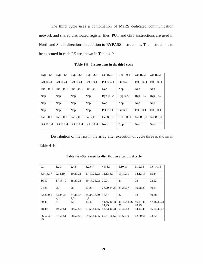
79
The third cycle uses a combination of MaRS dedicated communication
network and shared distributed register files. PUT and GET instructions are used in
North and South directions in addition to BYPASS instructions. The instructions to
be executed in each PE are shown in Table 4-9.
Table 4-8 – Instructions in the third cycle
Byp R,S4
Byp R,S4 Byp R,S4 Byp R,S4
Get R,0,1
Get R,0,1
Get R,0,1
Get R,0,1
Get R,0,1
Get R,0,1
Get R,0,1
Get R,0,1
Put R,0,-1
Put R,0,-1
Put R,0,-1
Put R,0,-1
Put R,0,-1
Put R,0,-1
Put R,0,-1
Put R,0,-1
Nop
Nop
Nop
Nop
Nop
Nop
Nop
Nop
Byp R,S2 Byp R,S2 Byp R,S2 Byp R,S2
Nop
Nop
Nop
Nop
Nop
Nop
Nop
Nop
Nop
Nop
Nop
Nop
Put R,0,1
Put R,0,1
Put R,0,1
Put R,0,1
Put R,0,1
Put R,0,1
Put R,0,1
Put R,0,1
Get R,0,-1
Get R,0,-1
Get R,0,-1
Get R,0,-1
Get R,0,-1
Get R,0,-1
Get R,0,-1
Get R,0,-1
Nop
Nop
Nop
Nop
Distribution of metrics in the array after execution of cycle three is shown in
Table 4-10.
Table 4-9 –State metrics distribution after third cycle
0,1
1,2,3 2,4,5 3,2,6,7 4,5,8,9 5,10,11 6,12,13 7,6,14,15
8,9,16,17
9,18,19 10,20,21 11,10,22,23
12,13,8,9 13,10,11 14,12,13 15,14
16,17
17,18,19 18,20,21 19,18,22,23
20,21 21 22 23,22
24,25
25 26 27,26 28,29,24,25 29,26,27 30,28,29 30,31
32,33 0,1
33,34,35 2,3
34,36,37 4,5
35,34,38,39 6,7
36,37 37 38 39,38
40,41
41 42 43,42 44,45,40,41 24,25
45,42,43,26 27
46,44,45 28,29
47,46,30,31
48,49
49,50,51 50,52,53 51,50,54,55
52,53,40,41
53,42,43 54,44,45 55,54,46,47
56,57,48 49
57,50,51 58,52,53 59,58,54,55
60,61,56,57
61,58,59 62,60,61 63,62

80
The fourth cycle again uses a combination of MaRS dedicated
communication network and shared distributed register files like cycle three. The
instructions to be executed in each PE are shown in Table 4-11.
Table 4-10 –Instructions in the fourth cycle
Nop
Nop
Nop
Nop
Byp R,S4
Byp R,S4 Byp R,S4 Byp R,S4
Byp R,S4
Byp R,S4 Byp R,S4 Byp R,S4 Byp S2,R Byp S2,R Byp S2,R Byp S2,R
Byp S2,R Byp S2,R Byp S2,R Byp S2,R
Byp S4,R Byp S4,R Byp S4,R Byp S4,R
Byp S4,R Byp S4,R Byp S4,R Byp S4,R
Byp S4,R Byp S4,R Byp S4,R Byp S4,R
Byp R,S2
Byp R,S2 Byp R,S2 Byp R,S2 Nop
Nop
Nop
Nop
Nop
Nop
Nop
Nop
Nop
Nop
Nop
Nop
Nop
Nop
Nop
Nop
Nop
Nop
Nop
Nop
Nop
Nop
Nop
Nop
Nop
Nop
Nop
Nop
Distribution of metrics in the array is shown in Table 4-12. After four
cycles, all of the new state metrics are transmitted to their corresponding successor
states as pointed out in blue.
Table 4-11 –State metrics distribution after fourth cycle
0,1
1,2,3 2,4,5 3,2,6,7 4,5,8,9 5,10,11 6,12,13 7,6,14,15
8,9,16,17
9,18,19 10,20,21 11,10,22 23
12,13,8,9 24,25
13,10,11 26,27
14,12,13 28,29
15,14,30 31
16,17,32 33
17,18,19 34,35
18,20,21 36,37
19,18,22 23,38,39
20,21,40 41
21,42,43 22,44,45 23,22,46 47
24,25,48 49
25,50,51 26,52,53 27,26,54 55
28,29,24 25,56,57
29,26,27 58,59
30,28,29 60,61
30,31,62 63
32,33,0,1
33,34,35 2,3
34,36,37 4,5
35,34,38 39,6,7
36,37,8,9 37,10,11 38,12,13 39,38,14 15
40,41,16 17
41,18,19 42,20,21 43,42,22 23
44,45,40 41,24,25
45,42,43 26,27
46,44,45 28,29
47,46,30 31
48,49,32 33
49,50,51 34,35
50,52,53 36,37
51,50,54 55,38,39
52,53,40 41
53,42,43 54,44,45 55,54,46 47
56,57,48 49
57,50,51 58,52,53 59,58,54 55
60,61,56 57
61,58,59 62,60,61 63,62
81
All of the operands are in the PE now; so the half trellis butterfly ACS
operation can be performed in each PE. This would be the fifth cycle.
There is an extra cycle needed to save the ACS flag in a register (packing
bits, either bit addressable register or the simple shift flag left instruction can be
used).
In order to be able to do trace-back concurrently while traversing trellis,
another PE is dedicated to performing trace-back. Every thirty-two iterations, all the
PEs send the trace-back data to the designated PE using a PUT instruction, and then
they immediately start their normal task. The designated trace-back PE will use the
“GET” instruction to receive the trace-back data after some cycles (totally hidden
latency) and concurrently will do the trace-back.
This is the first programmable solution capable of achieving the high rate
Viterbi decoder needed for IEEE 802.11a i.e. 54 Mbps. ASIC solutions has been
used in other implementations.
4.4.2 Mapping FFT on MaRS
FFT and FFT-like transformations are widely used in multimedia and
wireless communication applications; particularly, FFT is used in image processing
and wireless communication (multi-carrier modulation schemes), and DCT is used
in multimedia algorithms (image and video compression). The same FFT mapping
can be used for IFFT as well by conjugating the input and output, and for DCT with
minor modification in the twiddle factors.
The IEEE 802.11a WLAN standard requires a 64-point complex FFT. FFT
is considered a computation intensive application with a great level of inherent
82
parallelism; hence, it would be a good benchmark for MaRS performance
evaluation. Considering the results of our previous research work on MorphoSys,
we have adopted a radix-2 Decimation in Time 64-point complex FFT on an array
of PEs in MARS. In order to minimize the communication overhead, and
considering our experience from the previous mappings of FFT, we have chosen an
array of 2-by-8 of PEs for this mapping. As a rule of thumb, for each radix-2 stage
of FFT, one bit precision is required. So we use the packed 8-bit real, 8-bit
imaginary format of data. Decimation in Time algorithm requires bit-reversed
presorting which may easily be implemented for small-size FFT using the “divide
and conquer” approach.
The FFT butterfly operations are performed right after the presorting phase,
which follows a fixed order of operations: twiddle factors multiplication, data
communication, and addition/subtraction. Notice that the communication pattern
varies in different stages of the algorithm. In stages 1, 2, and 3 the FFT butterfly
needs to communicate with E-1/W-1, E-2/W-2 and E-4/W-4 respectively; however,
in stage 4 communication should be performed with S-1/N-1. For the last two
stages, no remote-PE communication is required. Considering the distributed shared
register files and routing network of the target platform, this communication pattern
is very friendly with MaRS.
The code to perform a 64-point complex FFT, including the presorting stage
has been developed and mapped on a 2 by 8 array of PEs in MaRS. The total
number of cycles is 108 including presorting. This gives us performance headroom
to do power optimization in our mapping or to free up some resources in case of
83
limited resources. The PE utilization in the presented mapping is estimated to be
82.3% excluding the pre-sorting stage.
As a potential future application, FFT may be needed for the emerging ultra-
wideband IEEE 802.15.3a WPAN standard (multi-band OFDM) as well. This
standard has not been ratified yet, but the OFDM alliance’s proposal requires a 128-
point FFT. Also the new WiMAX standard needs up to 2048 point FFT. The same
FFT takes 132 cycles on the TI C64x+ architecture using radix-4 algorithm.
84
Chapter 5 Reed Solomon Decoder
Reed Solomon Decoder
Another application with a lot of use in wired and wireless communication
is the Reed-Solomon decoder. For instance digital audio disc, or compact disc use
Reed-Solomon codes for error correction and error concealment. Reed-Solomon
code uses the Galois field properties and is a symbol based code i.e. groups of bits
are considered as a symbol. This makes them suitable to correct burst errors. The
Reed-Solomon is not a very good choice for the deep space telecommunication
systems because deep space channel does not usually induce burst errors in
transmitted data. It was discovered that when convolutional and Reed-Solomon
coeds are used in concatenated systems, enormous coding gains are achievable. A
convolutional code is used as an “inner code,” while a Reed-Solomon code is used
to correct errors at the output of the Viterbi decoder. The Viterbi decoder output
happens to have errors in burst (when decoder ended up in wrong state it will cause
a burst of error before recovering the correct state), providing the perfect match for
a Reed-Solomon code.
85
A Reed-Solomon decoder capable of correcting t errors with the symbol of
)(qGF has the following characteristics:
Block length: n=q-1
Number of parity-check symbols: n-k=2t
Minimum distance: dmin=2t+1
A Reed Solomon code of special interest is defined in the GF(256) as each
symbol corresponds to 8-bit i.e. one Byte which is the unit of storage. This makes
this class of Reed-Solomon codes very useful. The Reed-Solomon code with t=8
i.e. RS(255,239) and it is shortened versions are used in concatenation with
convolutional coding in many standards including DVB-T, DVB-H, and IEEE
802.16. This decoder is capable of correcting up to 8 GF symbols using 16 parity
symbols added to the transmitted data. In what follows the algorithm and
implementation of MaRS is explained simultaneously and an estimate for number
of cycles is presented and compared with other commercial DSP processors.
The encoder for Reed-Solomon is straightforward (it is simply dividing the
transmitted sequence by the characteristics polynomial and adding the remainder to
it) so it will not be discussed. For test purposes, the fact that all zero sequence is
codeword is used and errors are incorporated in the sequence and passed to the
decoder. This was part of the algorithm verification using Matlab. If the number of
errors is greater than 8 then the received sequence can not be decoded. The
architecture for Reed Solomon encoder is illustrated in Figure 5-1.
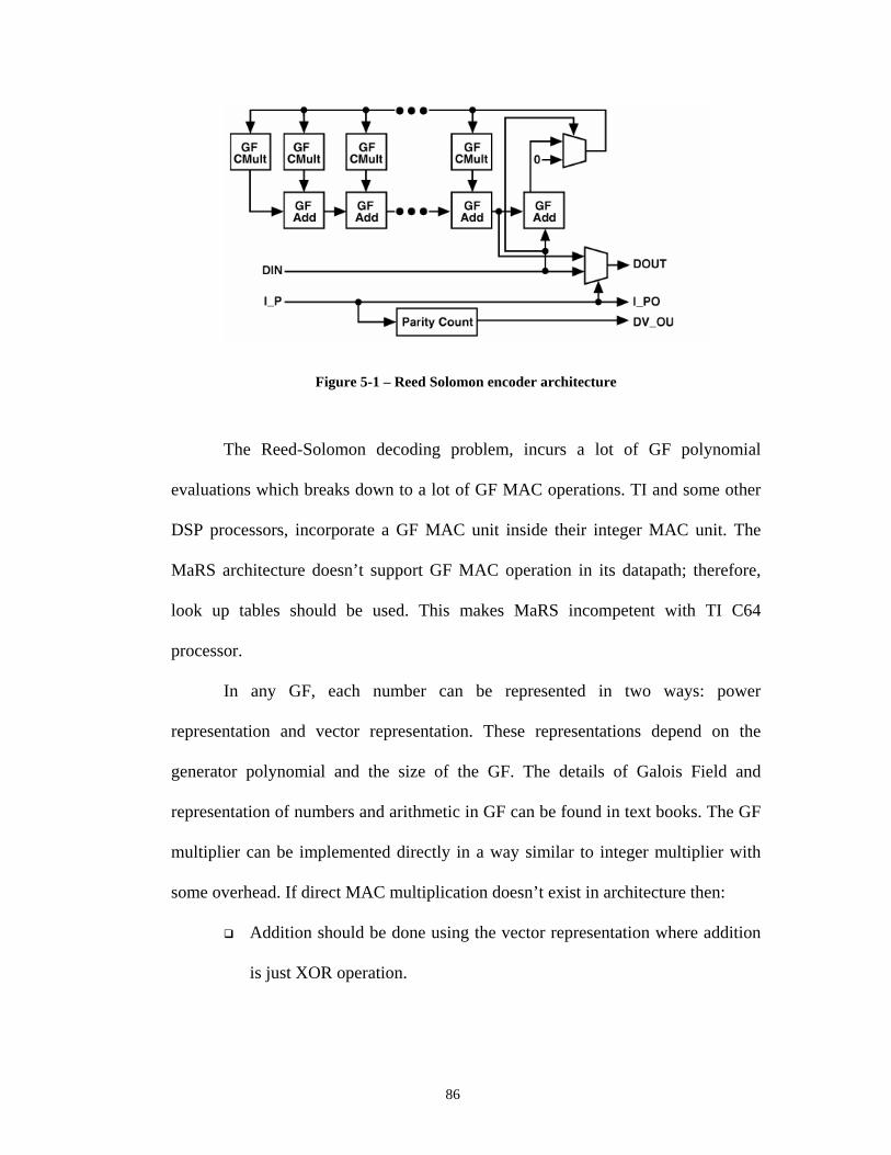
86
Figure 5-1 – Reed Solomon encoder architecture
The Reed-Solomon decoding problem, incurs a lot of GF polynomial
evaluations which breaks down to a lot of GF MAC operations. TI and some other
DSP processors, incorporate a GF MAC unit inside their integer MAC unit. The
MaRS architecture doesn’t support GF MAC operation in its datapath; therefore,
look up tables should be used. This makes MaRS incompetent with TI C64
processor.
In any GF, each number can be represented in two ways: power
representation and vector representation. These representations depend on the
generator polynomial and the size of the GF. The details of Galois Field and
representation of numbers and arithmetic in GF can be found in text books. The GF
multiplier can be implemented directly in a way similar to integer multiplier with
some overhead. If direct MAC multiplication doesn’t exist in architecture then:
Addition should be done using the vector representation where addition
is just XOR operation.

87
Multiplication should be done in power domain where it is just modulo
addition.
Therefore, assuming that original data is in vector format, for multiplication,
the multiplicands should be converted to their power representation using a look up
table. Modulo operation can be embedded in look up table as well. A simple
comparison and subtraction can be used interchangeably but adds a lot of overhead
to the number of cycles. The only problem with look up table is the size of tables to
be stored. This trade-off between number of cycles and memory to store tables
should be considered. The problem with size of the table is furthermore magnified
for MaRS implementation as each PE needs to keep its copy of the same table. In
this implementation, the Modulo-255 operation is performed using ALU
instructions in an attempt to reduce memory requirements. The decoding steps of
Reed-Solomon code can be enumerated in four steps [61-62].
5.1 Syndromes Computation
The first step in decoding RS code is to find the error syndromes. 2t error
syndromes should be computed where t is the number of symbols that the code can
correct. For the RS (255,239) code, syndromes are defined as:
( ) ( ) ∑∑==
===254
0
254
0 k
jkk
kj
kk
jj rrrS ααα Equation 5-1
Where j=1-16 and r is the received sequence. This formula can be written in
matrix form as well as shown in Equation 5-2 where the formula is expanded in
matrix form.
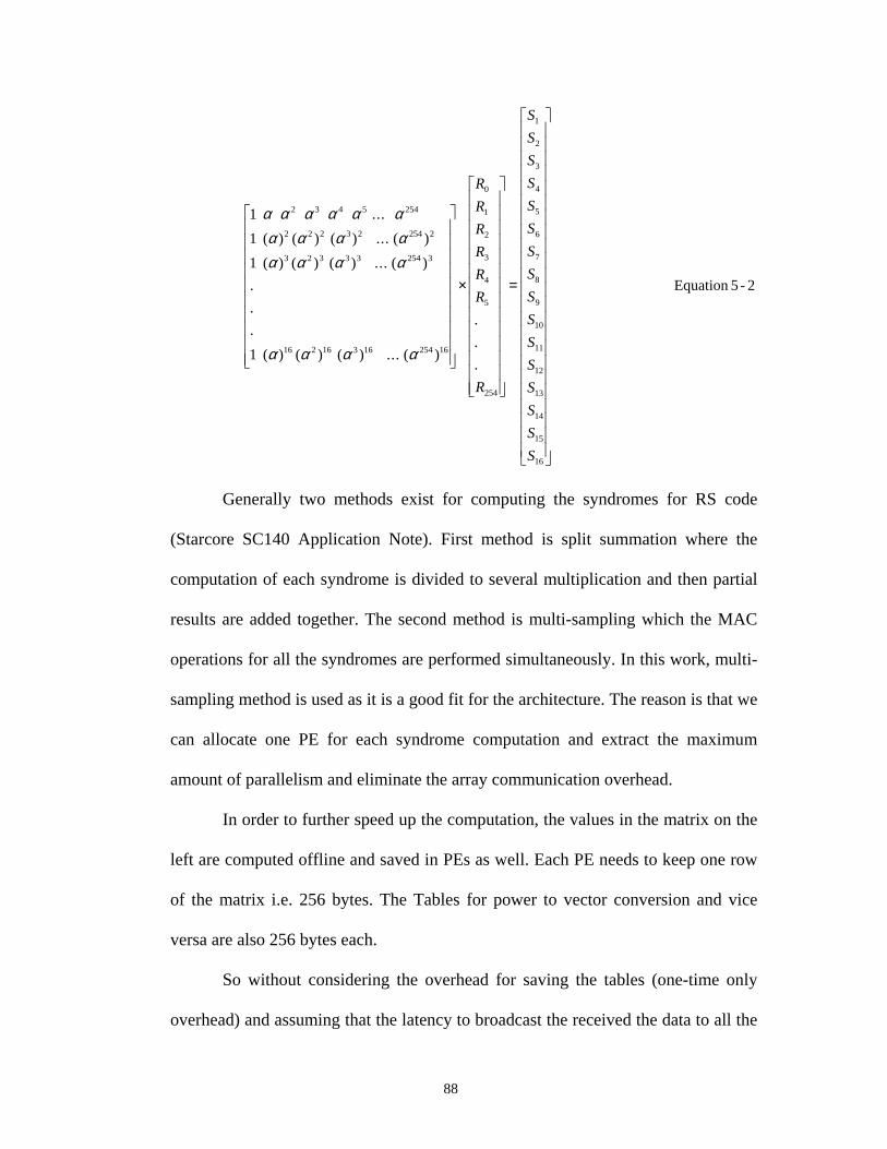
88
2-5 Equation
.
.
.
)(...)()()(1
.
.
.
)(...)()()(1
)(...)()()(1
...1
16
15
14
13
12
11
10
9
8
7
6
5
4
3
2
1
254
5
4
3
2
1
0
1625416316216
325433323
225423222
2545432
=
×
S
S
S
S
S
S
S
S
S
S
S
S
S
S
S
S
R
R
R
R
R
R
R
αααα
αααααααα
αααααα
Generally two methods exist for computing the syndromes for RS code
(Starcore SC140 Application Note). First method is split summation where the
computation of each syndrome is divided to several multiplication and then partial
results are added together. The second method is multi-sampling which the MAC
operations for all the syndromes are performed simultaneously. In this work, multi-
sampling method is used as it is a good fit for the architecture. The reason is that we
can allocate one PE for each syndrome computation and extract the maximum
amount of parallelism and eliminate the array communication overhead.
In order to further speed up the computation, the values in the matrix on the
left are computed offline and saved in PEs as well. Each PE needs to keep one row
of the matrix i.e. 256 bytes. The Tables for power to vector conversion and vice
versa are also 256 bytes each.
So without considering the overhead for saving the tables (one-time only
overhead) and assuming that the latency to broadcast the received the data to all the

89
PEs is hidden, the number of cycles needed for computing each syndrome is
estimated to be 2807. It should be noted that this is the worst case number as this
estimates assume the Modulo-255 operation should be performed in all iterations of
the loop.
5.2 Berlekamp Massey Algorithm
Once the syndromes are, the next phase of the algorithm should be
performed which is finding the error locator polynomial. This is a fully serial, fully
centralized algorithm which generally has 2t steps. For RS(255,239) it corresponds
to sixteen steps. Even though the Berlekamp Massey algorithm is fully serial in
essence, polynomial evaluation can be performed in parallel (each partial GF
multiplication can be done in parallel and then the results should be added together
i.e. split summation) it incurs a lot of communication overhead. In this
implementation, Berlekamp Massey algorithm is mapped into a single PE. This also
helps to have somehow balanced macro-block pipeline stages.
The PE in charge of this portion of the algorithm requires performing a lot
of GF MAC operations as well so the tables need to be loaded there as well. The
steps of Berlekamp Massey can be enumerated as:
1- Initialize the algorithm variables as follow: 0,1)(,0 )0( ==Λ= Lxk and .)( xxT =
2- Set k=k+1. Compute the discrepancy )(k∆ using: ik
l
i
kik
k SS −=
−∑Λ−=∆1
)1()(
3- If 0)( =∆ k , then go to 7.
4- Modify the error locator polynomial: )()()( )()1()( xTxx kkk ∆−Λ=Λ −
5- If kl ≥2 , then go to step 7.

90
6- Set LkL −= and )()1( /)()( kk xxT ∆Λ= −
7- Set )(.)( xTxxT = .
8- If tk 2< , then go to step 2.
9- Stop.
This algorithm is mapped on MaRS manually to get an estimated cycle
count for RS(255,239). Circular index is used to implement the shifting necessary
in the algorithm (multiplication by x). Code must be able to take care of exceptions
e.g. the case that more than 8 (generally degree of t) errors are introduced. The
Error locator polynomial will have a degree more than 8 (generally degree of t) in
that case. In order to save cycles and optimize the mapping, the discrepancy
computation part is coded individually for each stage (i.e. depending on the degree
of the polynomial to be evaluated).
Total number of cycles based on worst case scenario for this portion of Reed
Solomon decoding is estimated to be 3700 cycles, which 700 cycles are spent on
computing the discrepancy values.
5.3 Roots search (Chien search) algorithm
In this part of the algorithm, the roots of the error locator polynomial should
be found. The error locator polynomial has maximum degree of 8 (generally degree
of t). In order to find the roots, the polynomial should be evaluated with all the field
members; if the result is zero then a root is found. The polynomial has the form of:
( ) 88
77
66
55
44
33
2211 Β+Β+Β+Β+Β+Β+Β+Β+=ΒΛ σσσσσσσσ Equation 5-3
B should be substituted with all the values in the field i.e. α0-254. This
procedure can be performed in parallel as it consists of 255 independent

91
computations. In order to speed up the computation, a table containing pre-
computed all powers of α0-254 is used. It is important to note that this table would be
the same as top half of the matrix introduced in syndromes computation section
when accessed column-wise rather than row-wise (Equation 5-2). As the values of
σ1 to σ8 are used quite frequently, in the mapping they are saved in the registers.
Considering the aforementioned conditions, each evaluation takes 82 cycles.
So for 255 it would take 21676 taking into account the associated loop overhead.
This number is a lot compared to syndromes computation and will lead to
imbalanced pipeline stages if mapped to a single PE. If 16 PEs are used (i.e.
parallelism of 16) this part of the algorithm takes 1355 cycles and for 8 PEs tales
2710 cycles. This implementation uses 8 PEs for Chien search.
5.4 Forney Algorithm
In this part of the algorithm, Error location value can be found using the
following equation where Ω= Λ(1+S(x)) Mod x17and S(x) is the syndromes
polynomial.
)()(
1
1
−
−
Λ′ΧΩΧ−=k
kki X
ek
Equation 5-4
So the steps for the Forney algorithm are:
Calculating the Ω
Calculating Λ’
Evaluating Ω with the roots calculated in the last step
Evaluating Λ’ with the roots calculated in the last step and finding the
inverse
Multiplying them all together
92
The Chien search algorithm actually finds the roots in power format. So
finding the inverse is furthermore simplified (just a subtraction). In order to save
some cycles required to calculate the inverse of the roots the Chien search kernel
actually saves both Xk and Xk-1 simultaneously. Total number of cycles for Forney
algorithm implementation on MaRS single PE is estimated to be 2695 cycles.
5.5 Comparisons and Conclusion
This concludes the RS(255,239) algorithm mapping on MaRS architecture.
Consequently the kernels are chained to work in a macro-block pipeline fashion to
increase the throughput. Table 5-1 presents a comparison between MorphoSys,
Starcore SC 140, TI C64 and MaRS. The cycles for each part of the algorithm and
the grand total number of cycles are presented in the Table.
It should be noted that MaRS doesn’t have any special instruction or
datapath tailored for Reed Solomon decoding. Using the same mapping method, we
can implement different Reed-Solomon decoders on MaRS by changing the number
and allocation of the PEs and slight modification of the software. The allocation
depends to a great extent on the parameter t. MorphoSys and Starcore SC 140 use a
methodology very similar to MaRS as they don’t have any special instruction to
address Reed Solomon decoder. The MorphoSys implementation uses 8 of M2’s
reconfigurable cells for Reed Solomon decoding so can decode 8 blocks in parallel.
TI C64 gets a huge performance boost by incorporating a GF MAC unit to its
integer MAC unit. The area overhead is reported to be less than 10%.
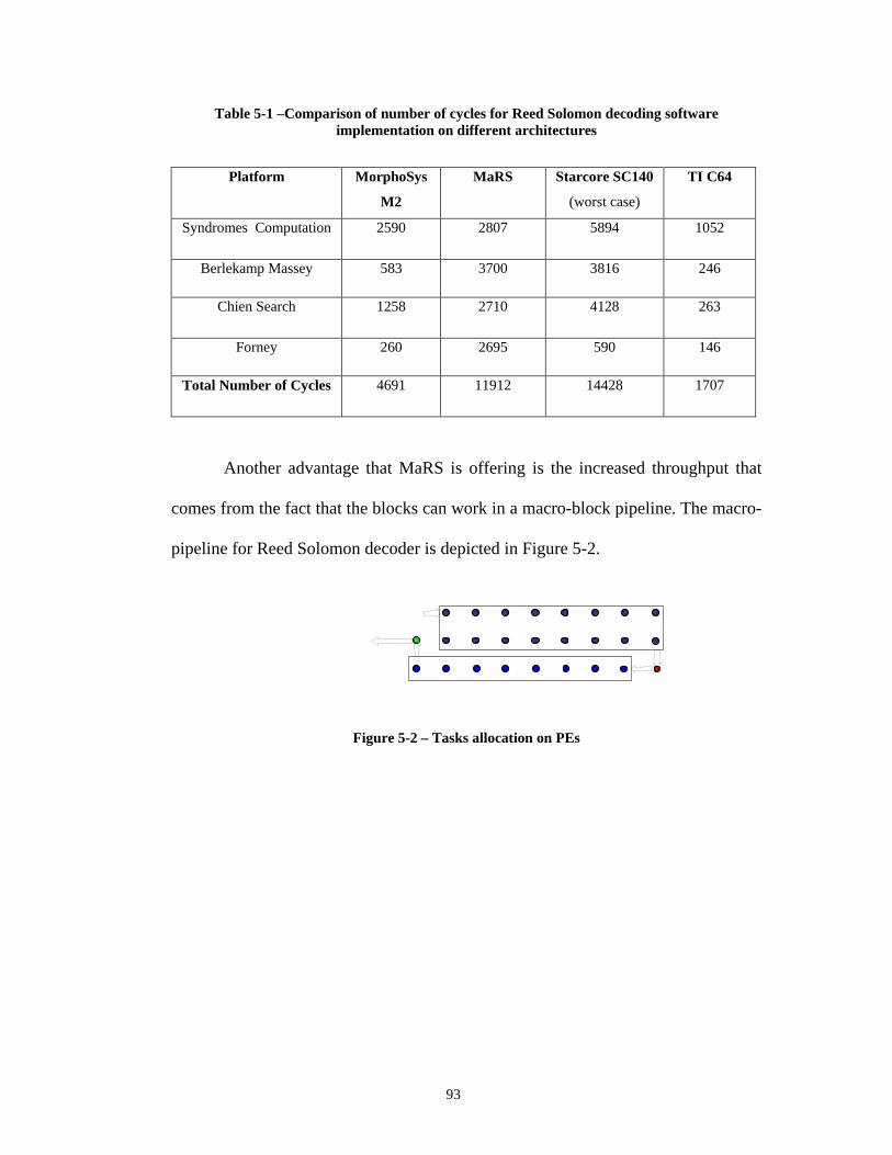
93
Table 5-1 –Comparison of number of cycles for Reed Solomon decoding software implementation on different architectures
Platform MorphoSys
M2
MaRS Starcore SC140
(worst case)
TI C64
Syndromes Computation 2590 2807 5894 1052
Berlekamp Massey 583 3700 3816 246
Chien Search 1258 2710 4128 263
Forney 260 2695 590 146
Total Number of Cycles 4691 11912 14428 1707
Another advantage that MaRS is offering is the increased throughput that
comes from the fact that the blocks can work in a macro-block pipeline. The macro-
pipeline for Reed Solomon decoder is depicted in Figure 5-2.
Figure 5-2 – Tasks allocation on PEs
94
Chapter 6 Implementation of Parameterized Viterbi Decoder in MaRS
Implementation of Parameterized Viterbi Decoder in MaRS
In today’s wireless communication system, usually convolutional codes and
convolutional turbo codes are used as the forward error correction scheme.
Concatenation of Reed-Solomon and convolutional code is also used to get a good
performance. The details of the Reed-Solomon code has been presented in the
previous chapter and the requirements for the mapping were presented. It was
shown that by having GF (256) MAC unit and powerful memory interface, the
number of cycles can be reduced considerably. In this chapter, the focus is on CC
and CTC as they are both based on trellis diagram.
Maximum likelihood decoding of turbo codes, requires a soft-input soft-
output (SISO) unit which is computationally intensive and makes the VLSI
implementation difficult. The sub-optimal methods have been presented to reduce
the complexity of decoders for turbo codes. A very popular sub-optimal method is
MAX_LOG_MAP algorithm. With the introduction of duo-binary turbo codes, the
trellis traversal computation is getting even more complicated; hence, using the

95
MAX_LOG_MAP method makes more sense. The MAX_LOG_MAP method is
very similar to Viterbi algorithm for convolutional codes. This is the motivation to
look at these algorithms and find the commonality between them as far as the VLSI
implementation is concerned.
6.1 Convolutional Codes
Convolutional code consists of a feed-forward shift register with size K-1
where K is called constraint length, and it gets ‘k’ input and generates ‘n’ out i.e.
rate k/n. The design of feed-forward locations is the topic of code design as bad
location can lead to catastrophic convolutional codes with poor performance. The
output of the convolutional encoder depends on the input and current state of the
encoder. A convolutional code can be systematic or non-systematic. In a systematic
code, the input appears in the input and the redundancy is added to it.
A convolutional code can fully be represented by its trellis diagram as well.
The trellis diagram shows the transition from all the states corresponding to all
possible inputs and their corresponding outputs. Encoder by looking at the trellis,
knowing the current state and the input can generate the output and decoder
basically traverses the trellis to decode the data sequence. The number of input bits
to the encoder i.e. value k, is a measure of the trellis complexity. There are 2k
branches leaving and entering each node of the trellis. The number of nodes equals
to the number of states i.e. 2(K-1). Figure 6-1 shows a parameterized trellis diagram
of a convolutional code.
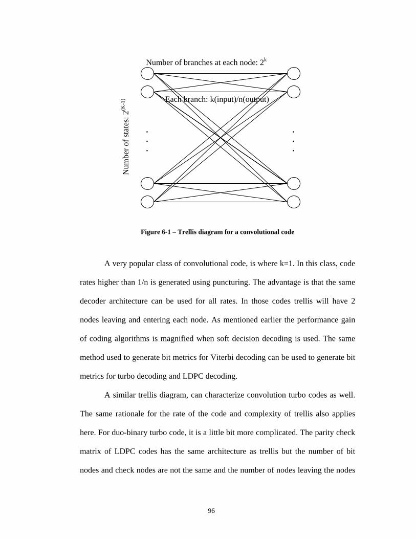
96
Figure 6-1 – Trellis diagram for a convolutional code
A very popular class of convolutional code, is where k=1. In this class, code
rates higher than 1/n is generated using puncturing. The advantage is that the same
decoder architecture can be used for all rates. In those codes trellis will have 2
nodes leaving and entering each node. As mentioned earlier the performance gain
of coding algorithms is magnified when soft decision decoding is used. The same
method used to generate bit metrics for Viterbi decoding can be used to generate bit
metrics for turbo decoding and LDPC decoding.
A similar trellis diagram, can characterize convolution turbo codes as well.
The same rationale for the rate of the code and complexity of trellis also applies
here. For duo-binary turbo code, it is a little bit more complicated. The parity check
matrix of LDPC codes has the same architecture as trellis but the number of bit
nodes and check nodes are not the same and the number of nodes leaving the nodes
.
.
.
.
.
.
Num
ber
of s
tate
s: 2(K
-1)
Number of branches at each node: 2k
Each branch: k(input)/n(output)

97
on the left and right are not equal. It should be noted that trellis architecture is a
highly used concept in communication theory and is also used in TCM, DOPSK
demodulation, trellis space time code, LDPC code and etc. Generally every linear
code can be shown using a trellis diagram, but for block codes easier decoding
methods exist.
For soft decoding of convolution codes, Viterbi algorithm should be used.
Viterbi algorithm is a maximum likelihood method to decode convolution codes.
The basic idea is to find the path in trellis with the maximum possibility. A brute
force search method is extremely inefficient and computationally intensive. Viterbi
decoding algorithm uses dynamic programming concept to minimize the necessary
computation. In Viterbi algorithm, the trellis is traversed for all the input symbols.
It is proven that if the starting and finishing states are known the code performance
is the best (free distance is more). Usually, the encoder starts from state zero and
the data is padded with K-1 zeros to guarantee that encoder finishes at state zero as
well. The decoder then uses this knowledge to decoder the data. The problem with
this method is the rate loss introduced by using the tail bits. For short blocks of data
and for codes with K as big as 7 this overhead can’t be ignored. There is another
method i.e. tail biting, where the encoder is initialized with the K-1 last bits of data.
This method eliminates the pad bits, but it has its own problems. First of all, the ML
decoding is a lot more complicated as the decoding must be done on the number of
states which is impractical, therefore, sub-optimal methods should be used.
Moreover, tail biting incurs encoding delay and decoding delay as the trellis must

98
be traversed more than once. In what follows, the decoding of zero tailing method is
described as the main part which is the traversal part is the same for both methods.
For a rate 1/n code with constraint length K, the first step in trellis traversal
is to calculate branch metrics. At each stage, the decoder needs n soft input. The
total number of possible branch metrics is 2n. The branch metrics are all possible
combinations of received soft metrics. Assuming that the soft bit metrics to zero are
the input to the decoder, the branch metric will look like:
n transitioa toingcorrespond ueoutput val theis:
zero respect to with metric-bitsoft received theis:
)21(1
i
i
valuesipossibleallforiiMetricBranch k
n
kkk
)
)
∑=
−=
Equation 6-1
At start, a metric is associated to each state. In zero tailing, it is known that
that the trellis has started from state zero, in order to enforce that, the metric of state
zero is initialized with a very large negative number and all other states are
initialized with zero. At each state, all the possible new metrics are computed by
adding the possible previous states’ metric to the corresponding branch metric. The
path with the minimum metric will be selected and the metric associated to that path
will be assigned to the state in the branch metric update phase (the value should not
be overwritten). This operation is called Add-Compare-Select (ACS) as it consists
of an addition comparison and selecting the minimum. For a constraint length K
rate k/n convolution code the trellis traversal will look like Figure 6-2.

99
Figure 6-2 – Trellis traversal for convolutional code with rate k/n
The relation between possible previous states and the current states is given
by 0111011 ............ aaaaxxaaa knnkkn −−−− → for all combinations of x1 and xk.
Therefore the computation needed for trellis traversal part of Viterbi
algorithm can be summarized as:
Calculation of Gamma + 2(K-1) Each Node ACS + Trace Back Overhead
It should also be noted that for tail biting code there will be an overhead in
the prologue to find the initial values of the metrics. Table-6-1 elaborates on the
cycle counts for Viterbi decoding computation.
.
.
.
Pos
sibl
e pr
evio
us s
tate
s: 2
k
Gamma1
Gamma2
Gamma2k
Gamma2k-1

100
Table 6-1 –Computation breakdown for decoding of 1-bit using Viterbi decoder
Kernel Computation
Calculation of Gamma 2n-1.(n-1) Addition1
2(K-1) * Each Node ACS 2(K-1).[ 2k Add+ (2k-1) Compare2]
Trace Back Overhead 2(K-1).[1 to save TB bit]
Trace Back Read TB bits + Find Previous State(LUT) + Decode k bits3
1- Considering the fact that half of the metrics are negative of others and assuming two input
additions
2- 2k input comparisons are assumed to have the cost of 2k-1 two-input comparators
3- It is assumed that trace-back is done only once at the end so finding the state with best
metric is not necessary.
To get a better idea about the typical amount of computations required to
decode one bit, let’s consider the widely used case of n=1, k=2, K=7 convolution
code with [133,171]. The number of computations to decode one bit is illustrated in
Table 6-2.
Table 6-2- Instructions break-down for decoding one bit using Viterbi algorithm
# of times Cycles Break-down
1 2 Additions for BM computation 64 4 2 ADD + 1 Compare + 1 TB bit handling
1 1 Access TB bit 1 1 Look up previous state 1 1 Decode bit
Total 261
This is actually the lower bound of instructions needed and excludes the
overhead to load the data and the overhead of updating branch metrics which can be
huge for distributed computing. For IEEE 802.11a, the rate is 54 Mbps which
corresponds to about 14.1 GIPS!

101
In order to reduce the GIPS requirement, several ways exist:
1. Use the parallelism in the algorithm i.e. trellis computation at each
node is totally independent of other nodes.
2. Augment the ISA with specific instructions and data-path to
combine several instruction into one instruction e.g. Add-Compare-
Select (ACS).
3. Pipelining in way that data is partitioned into several blocks, then the
latency of trace-back can be hidden i.e. trace-back of first block is
concurrent with trellis traversal of second block.
A combination of all mentioned solutions should be used in order to get a
reasonable MIPS for this application.
6.1.1 Data Communication Pattern
In the discussion so far, it is assumed that data communication is performed
using shared memory system i.e. the branch metric update doesn’t need extra cycle.
For ASIC processors this is not a problem as well because fixed wires can facilitate
the data communication pattern. Data communication turns out to be the bottleneck
in array processors with simple single layer data communication network.
6.2 Convolutional Turbo Code
Turbo codes are a class of recently-developed high-performance error
correction codes finding use in deep-space satellite communications and other
applications where achieving maximal information transfer over a limited-
bandwidth communication link in the presence of noise and interference is desired.
102
Of all practical error correction methods known to date, turbo codes,
together with Low-density parity-check codes, come closest to approaching the
Shannon limit, the theoretical limit of maximum information transfer rate over a
noisy channel. Its main drawbacks are the relative high decoding complexity and
relatively high latency, which makes it unsuitable for some applications.
Turbo coding was first introduced by French engineers, Berrou, Glavieux,
and Thitimajshima in their 1993 paper [63]. Turbo code refinements and
implementation are still an area of active research.
The encoder sends three sub-blocks of bits. The first sub-block is the m-bit
block of payload data. The second sub-block is n/2 parity bits for the payload data,
computed using a convolutional code. The third sub-block is n/2 parity bits for
interleaved payload data, again computed using the same or another convolutional
code. The complete block has m+n bits of data with a code rate of m/(m+n).
Turbo codes are used extensively in 3G mobile telephony standards. The
problem with the turbo code is the complexity of the decoding which is performed
in an iterative fashion.
6.2.1 CTC Encoding
The encoding part consists of two parts. First the data is passed through the
first encoder. Then the interleaved data is passed through the second encoder which
can be similar or different from the first encoder. Then another layer of interleaving
is performed on top of that. And then puncturing can be performed if necessary.
103
Most of the discussion presented in the Viterbi decoding can be applied to
turbo decoding as well. Each constituent encoder can be represented by its trellis
diagram and the decoding can be done by traversing the trellis diagram.
Circular coding is an adaptation of tail-biting in convolutional codes to
recursive convolutional turbo codes. It ensures that at the end of encoding
operation, the encoder retrieves the initial state, so that data encoding can be
represented by a circular trellis. Pre-coding, codes the data assuming that it starts
from state zero and finishing in an intermediate state and consequently from a table
the circulation state is found. The overhead here is the necessity to code the data
twice; once to find the circulation states and second time for actual encoding.
6.2.2 Turbo Decoder
Iterative decoding of Turbo codes is usually performed using BCJR
algorithm [65]. The decoder for a convolutional turbo code is illustrated in Figure
6-3. The Soft-Input Soft-Output (SISO) block is the core of the turbo decoder. The
SISO decoder operation finds the likelihood of the input sequence given the
received sequence. The SISO element contains a lot of computation, therefore
usually instead of likelihood, log likelihood ratio (LLR) measure is used. Even the
LLR operation is very complicated in most of the cases and usually sub-optimal
algorithms such as max-log-MAP are used in VLSI implementation of turbo
decoders. Particularly with duo-binary turbo code being used extensively max-log-
MAP is the only method with reasonable computation load. The theoretical
background is beyond the scope of this dissertation and is a well understood topic.
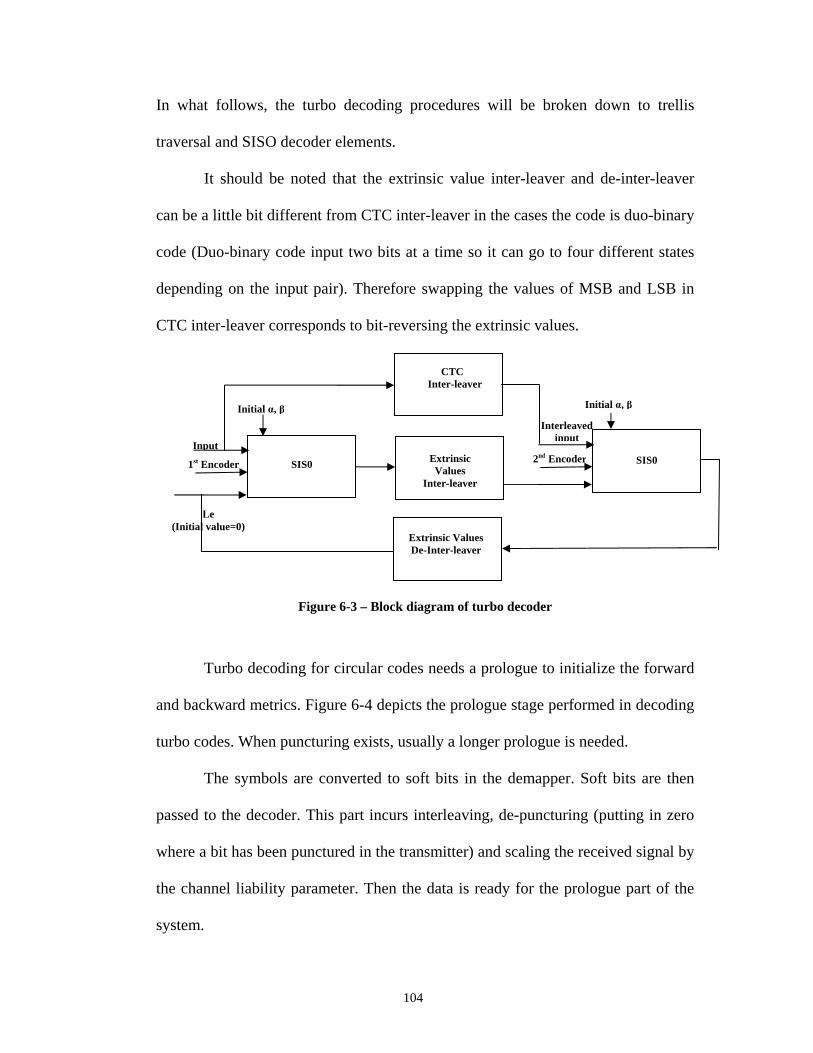
104
In what follows, the turbo decoding procedures will be broken down to trellis
traversal and SISO decoder elements.
It should be noted that the extrinsic value inter-leaver and de-inter-leaver
can be a little bit different from CTC inter-leaver in the cases the code is duo-binary
code (Duo-binary code input two bits at a time so it can go to four different states
depending on the input pair). Therefore swapping the values of MSB and LSB in
CTC inter-leaver corresponds to bit-reversing the extrinsic values.
Figure 6-3 – Block diagram of turbo decoder
Turbo decoding for circular codes needs a prologue to initialize the forward
and backward metrics. Figure 6-4 depicts the prologue stage performed in decoding
turbo codes. When puncturing exists, usually a longer prologue is needed.
The symbols are converted to soft bits in the demapper. Soft bits are then
passed to the decoder. This part incurs interleaving, de-puncturing (putting in zero
where a bit has been punctured in the transmitter) and scaling the received signal by
the channel liability parameter. Then the data is ready for the prologue part of the
system.
SIS0
Input
1st Encoder SIS0
Interleaved input
2nd Encoder Extrinsic Values
Inter-leaver
CTC Inter-leaver
Extrinsic Values De-Inter-leaver
Initial α, β Initial α, β
Le (Initial value=0)
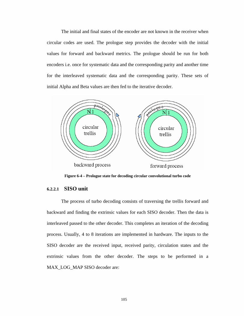
105
The initial and final states of the encoder are not known in the receiver when
circular codes are used. The prologue step provides the decoder with the initial
values for forward and backward metrics. The prologue should be run for both
encoders i.e. once for systematic data and the corresponding parity and another time
for the interleaved systematic data and the corresponding parity. These sets of
initial Alpha and Beta values are then fed to the iterative decoder.
Figure 6-4 – Prologue state for decoding circular convolutional turbo code
6.2.2.1 SISO unit
The process of turbo decoding consists of traversing the trellis forward and
backward and finding the extrinsic values for each SISO decoder. Then the data is
interleaved passed to the other decoder. This completes an iteration of the decoding
process. Usually, 4 to 8 iterations are implemented in hardware. The inputs to the
SISO decoder are the received input, received parity, circulation states and the
extrinsic values from the other decoder. The steps to be performed in a
MAX_LOG_MAP SISO decoder are:

106
• Branch metric, Gamma values should be computed. This is very similar
to the Viterbi decoder; however the extrinsic values from other decoder
are added to the metric as well.
• Next step is traversing the trellis forward and computing the Alpha
values. This part for MAX_LOG_MAP algorithm is simple and is
similar to Viterbi decoder. For each path entering a trellis node the
metric equal to the previous state added to path metric is calculated and
the maximum value is found. The initial values of Alpha are set in a way
to force the trellis start from circulation state.
• The final step is to trace backward, and compute the Beta values. Beta
values are computed in a similar manner to Alpha values, just traversing
the trellis backward.
• Final step is finding the extrinsic values using Alphas, Betas and
Gammas. This part for each possible input combination all the possible
transitions are found and the one leading to maximum value is selected.
107
Chapter 7 Conclusions
Conclusions
The MaRS architecture was presented as a programmable solution for DSP
and wireless communication applications as an example of architecture-application
co-design. The target application is the IEEE 802.11a wireless LAN receiver
including the FEC decoder. To this end, a comprehensive system simulation model
using Matlab was developed and consequently mapped on MaRS architecture.
Functional simulations were performed in RTL level using hand-optimized
assembly code. Moreover an object oriented cycle accurate simulator C++
simulator was developed to speed-up verification and debugging process.
7.1 Contributions
The contributions of dissertation are as follows:
• A fully IEEE 802.11a compliant TX, Channel and RX simulator is
presented.
• VLSI-friendly synchronization algorithms for IEEE 802.11a receiver
are developed and tested. Fixed-point Matlab system simulations are
also performed to define the precisions needed for parameters.
108
• A novel timing synchronization method using short training
sequences is presented that reduces the synchronization time and
computations needed.
• A soft decision decoder for bit interleaved coded modulation scheme
using sub-optimal method applying channel state information is used
and considerable gain as high as 8 dB are achieved.
• The MaRS architecture, including its PE architecture,
communication network, ISA, and programming model is presented.
• Augmentation to ISA and micro-architecture for Viterbi decoder and
FFT are presented.
• Datapath and accelerators are presented for the target applications.
• MaRS performance is evaluated for the selected applications.
• Performance of MaRS for widely used FEC coding algorithm is
studied.
• IEEE 802.11a receiver kernels are partitioned and mapped on the
MaRS architecture.
• The first single chip fully programmable receiver for IEEE 802.11a
is presented.
7.2 Future Direction of MaRS
The experience gained from mapping different applications and algorithms on
the MARS architecture has pointed out some of the points that MaRS architecture
can be refined. As a very good example, while mapping the Reed-Solomon decoder
on the architecture, we noticed that 30% of the processing time is dedicated to the
109
loop overhead. By using a zero overhead looping buffer to keep the address of the
target of branch instruction this overhead can be eliminated. Zero overhead looping
technique is being utilized in most of the state of art DSP processors as well and the
micro-architecture overhead is minimal. This is something that next generation of
MaRS should support. It was also noticed that for applications with intra-PE data
dependencies, a lot of cycles are spent for memory access. This latency can be
hidden most of time by loop unrolling and supporting a very simple VLIW
architecture. A proposed architectural modification is two have a 2-slot VLIW
where one slot is allocated to functional units and one slot is allocated to memory
access. This will save us a lot of cycle for an application such as RS decoder or any
other application with a lot of look up table. Another noticeable shortcoming in the
current MaRS architecture is that it only has one Index register. This can be a
bottleneck for an application such as RS decoder with different tables and access
patterns. Developing tools such as assembler and compiler is an integral part of any
platform design project which consumes a lot of resources. An efficient solution is
to replace the current PE with an open source RISC architecture where some of the
already existing tools and compilers can be used. The compiler design for MaRS is
still an ongoing process by researchers in advanced computer architecture lab.
MaRS automated programming flow currently being considered allows the
programmer to code the application in either a streaming language with explicit
communication, or manually partitioned and mapped sequential C. The current
front-end reads an application written in “Streamit” . After converting the
application to an intermediate representation, the compiler splits or merges the

110
kernels to adapt the granularity of the application to the MaRS, and maps the
partitioned kernels to the PEs. The kernels mapped to the PEs are converted to C
programs. A Java program is generated from the Streamit application for functional
simulation.
The programmer can also manually partition the application by writing a C
code for each virtual PE with message passing function calls to specify
communications between PEs. Virtual PE to physical PE mapping is specified in a
separate configuration file. The C programs are converted to threads for functional
simulation. The C programs, either generated by the Streamit compiler or manually
by the programmer, are compiled by a uni-processor compiler based on the
SUIF/MachSUIF compiler infrastructure, which generates machine code for each
PE. The library for application specific PEs still needs a lot of enhancements. Even
though we have been focused on programmability and generality, but the fact is that
for some application with stringent power and performance requirements, ASIC is
preferable. An example would be Viterbi decoder for high rate application such as
Wireless Personal Area Networks requiring bit rates in the order of hundreds of
mbps or turbo decoders. Another area that we have to attack is CDMA algorithms.
Even though OFDM has been the de facto modulation scheme in almost all of the
new wireless standards, but seems like CDMA will still be around at least for a
decade or so with the deployment of high speed extensions of 3G.
Because of the lack of funding, the actual implementation of the MaRS in
silicon is not considered in near future. Low power techniques in VLSI

111
implementation and system level management are issues that should be considered
in the design and back-end optimization.
112
Bibliography [1] http://ieee802.org/11/ [2] http://ieee802.org/15/ [3] http://ieee802.org/16/ [4] http://en.wikipedia.org/wiki/CDMA [5] ETSI Specification EN 302 304 "Transmission System for Handheld Terminals (DVB-H)" (this will open ETSI document search engine, to download the latest version of the document enter a search string "EN 302 304") [6] ETSI Technical Report TR 102 377 "DVB-H Implementation Guidelines" (this will open ETSI document search engine, to download the latest version of the document enter a search string "TR 102 377") [7] ETSI Technical Report TR 102 401 "DVB-H Validation Task Force Report" (this will open ETSI document search engine, to download the latest version of the document enter a search string "TR 102 401") [8] Hartej Singh, Ming-Hau Lee, Guangming Lu, Fadi J. Kurdahi, Nader Bagherzadeh, and Eliseu M. C. Filho , “MorphoSys: An Integrated Reconfigurable System for Data-Parallel and Computation –Intensive Applications,” IEEE Trans. Computers, Vol. 49, No. 5, pp. 465-481, May 2000. [9] C. Pan, N. Bagherzadeh, A.H. Kamalizad, A. Koohi, "Design and analysis of a programmable single-chip architecture for DVB-T base-band receiver," in Proceedings of Design, Automation and Test in Europe (DATE03), pp. 468-473, Munich, Germany, March 3-7, 2003. [10] A.H. Kamalizad, C. Pan and N. Bagherzadeh, "A Very Fast 8192-Point Complex FFT Implementation Using MorphoSys Reconfigurable DSP," in Proceedings of 15th Symposium on Computer Architecture and High Performance Computing, SBAC-PAD 2003, pp. 254-258, São Paulo, SP – Brazil, November 10-12, 2003. [11] A. Koohi, N. Bagherzadeh, C. pan, "A Fast Parallel Reed-Solomon Decoder on a Reconfigurable Architecture," CODES+ISSS, pp. 59-64, Newport Beach, California, October 1-3, 2003. [12] Manuel L. Anido, Nozar Tabrizi , Haitao Du , Marcos Sanchez-Elez M., Nader Bagherzadeh, “Interactive Ray Tracing Using a SIMD Reconfigurable Architecture,” in Proceedings of the 14th Symposium on Computer Architecture and High Performance Computing, SBAC-PAD, Vitoria/ES – Brazil, October 28-30, 2002. [13] N. Tabrizi, N. Bagherzadeh, A. Kamalizad, H. Du, “MaRS: A Macro-pipelined Reconfigurable System,” To Appear in ACM Computing Frontiers, Italy, 2004. [14] Kamalizad, Tabrizi, Bagherzadeh, “MaRS: A Programmable DSP architecture for wireless communication systems,” to appear in IEEE ASAP 2005. [15] Supplement to IEEE standard for information technology telecommunications and information exchange between systems - local and metropolitan area networks - specific requirements. Part 11: wireless LAN Medium Access Control (MAC) and Physical Layer (PHY) IEEE Std. 802.11a-1999, 1999.

113
[16] A. Kamalizad, N. Bagherzadeh, “Performance of Soft Decoding Using Channel State Information in IEEE 802.11a,” Accepted for publication in VTC Fall 2004. [17] A. Kamalizad, N. Bagherzadeh, “Synchronization Algorithms for IEEE 802.11a Receiver,” Accepted for publication in VTC Spring 2004. [18] http://www.eembc.org [19] http://www.intel.com/technology/mooreslaw/index.htm [20] http://www.pactcorp.com/ [21] Michael Bedford Taylor, et al, “The RAW Microprocessor: A Computational Fabric for Software Circuits and General-Purpose Programs,” IEEE Micro Volume: 22 Issue: 2 , pp. 25 -35, March-April 2002. [22] http://www.ipflex.com/en/ [23] http://focus.ti.com/dsp/docs/dsphome.tsp?sectionId=46 [24] R. Simar Jr, “CODEVELOPMENT OF THE TMS32OC6X VelociTI ARCHITECTURE AND COMPILER” [25] http://www.starcore-dsp.com [26] M. Tremblay and J. M. O’Connor, “UltraSparc I: A four-issue processor supporting multimedia,” IEEE Micro, vol. 16, pp. 42–50, Apr. 1996. [27] S. K. Raman, V. Pentkovski, and J. Keshava, “Implementing streaming SIMD extensions on the Pentium III processor,” IEEE Micro, vol. 20, pp. 47–57, July/Aug. 2000. [28] S. Thakkur and T. Huff, “Internet streaming SIMD extensions,” Computer, vol. 32, no. 12, pp. 26–34, Dec. 1999. [29] http://www.motorola.com/SPS/PowerPC/AtiVec/facts/.html [30] R. B. Lee, “Subword parallelism with MAX-2,” IEEE Micro, vol. 16, pp. 51–59, Aug. 1996. [31] http://www.analog.com/processors/processors/tigerSHARC/whitePapers/newArch.html [32] Raphael David, et al, “A Dynamically Reconfigurable Architecture Dealing with Future Mobile Telecommunications Constraints,” in proceedings of Parallel and Distributed Processing Symposium, IPDPS, pp. 156 -163, 15-19 April 2002. [33] Michael Bedford Taylor, et al, “THE RAW MICROPROCESSOR: A COMPUTATIONAL FABRIC FOR SOFTWARE CIRCUITS AND GENERAL-PURPOSE PROGRAMS,” IEEE Micro Volume: 22 Issue: 2 , pp. 25 -35, March-April 2002. [34] H. Du Ph.D. Dissertation [35] C. Pan Ph.D. Dissertation [36] Kamalizad, R. Plettner, C. Pan, N. Bagherzadeh, “Fast Parallel Soft Viterbi Decoder Mapping on a Reconfigurable DSP Platform,” IEEE SoC conference, 2004. [37] R. Plettner, " ," M.Sc. Thesis UC Irvine EECS Department
114
[38] N. Tabrizi, N. Bagherzadeh, "Bitonic Sorter Implementation," Technical Report, UC Irvine EECS department [39] L. Ni, P.K. McKinley, "A survey of wormhole routing techniques in direct networks," IEEE Computer 26(2), pp. 62-76, 1993. [40] H. S. Stone, “Parallel Processing with the Perfect Shuffle,” Computers, IEEE Transactions on, Vol.20, No.2, pp.153-161, Feb 1971. [41] http://www.artisan.com/ [42] A.V. Oppenheim, A. Willsky, S.H. Nawab, Signals and Systems, 2nd Edition, Prentice-Hall, 1996 [43] http://www.spec.org/ [44] http://www.icsl.ucla.edu/~billms/Publications/mediabench.pdf [45] http://www.eecs.umich.edu/mibench/ [46] J. Proakis, Digital Communications, Fourth Ed., McGraw Hill, 2000 [47] H. Hashemi, “The indoor radio propagation channel,” Proc. IEEE, vol. 81, pp. 943–968, July 1993. [48] A. A. M. Saleh and R. A. Valenzuela, "A statistical model for indoor multipath propagation," IEEE J. Sel. Areas Commun., vol. SAC-5, no. 2, pp. 128--137, Feb. 1987 [49] N. Chayat, “Tentative Criteria for Comparison of Modulation Methods,” IEEE P802.11–97/96. [50] Heinrich Meyr, Marc Moeneclaey and Stefan A. Fechtel, “Digital Communication Receivers,” Wiley, 1998. [51] M. Speth, S.A. Fechtel, G. Fock, H. Meyr, “Optimum receiver design for wireless broad-band systems using OFDM Part I,” Communications, IEEE Transactions on, Vol.47, No.11, pp. 1668-1677, Nov. 1999. [52] P. Moose, “A technique for orthogonal frequency division multiplexing frequency offset correction,” Communications, IEEE Transactions on, Vol.42, No.10, pp. 2908 -2914, Oct. 1994. [53] T. Schmidl, D. Cox, “Robust frequency and timing synchronization for OFDM,” Communications, IEEE Transactions on, Vol.45, No.12, pp. 1613 -1621, Dec 1997. [54] C. Peng, K. Wen, “Synchronization for carrier frequency offset in wireless LAN 802.11a system,” Wireless Personal Multimedia Communications, The 5th International Symposium on, Vol.3, pp.1083 -1087, 2002. [55] http://www.dvb.org [56] http://www.worlddab.org [57] J. Thomson, et al., “An integrated 802.11a baseband and MAC processor,” ISSCC 2002, pp. 126 -451, vol.1, 2002. [58] E. Zehavi, “8-PSK trellis codes for a Rayleigh channel,” Communications, IEEE Transactions on, Vol.40, No.5, pp.873-884, May 1992.

115
[59] G. Caire, G. Taricco, E. Biglieri, “Bit-interleaved coded modulation,” IEEE Transactions on Information Theory, Vol.44, No.3, pp.927-946, May 1998. [60] F. Tosato, P. Bisaglia, “Simplified soft-output demapper for binary interleaved COFDM with application to HIPERLAN/2,” Communications, Proceedings of IEEE International Conference on, Vol.2, pp. 664-668, May 2002. [61] Shung, Siegel, Ungerboeck, Thapar, " VLSI architectures for metric normalization in the Viterbi algorithm," Communications, 1990. ICC 90, Including Supercomm Technical Sessions. SUPERCOMM/ICC '90. Conference Record., IEEE International Conference on 16-19 April 1990 Page(s):1723 - 1728 vol.4 [62] Wicker, "Error Control Systems for Digital Communication and Storage", Prentice-Hall 1995 [63] Lin and Costello, "Error Control Coding: Fundamentals and Applications", Prentice-Hall 1983 [64] BERROU, C., GLAVIEUX, A., and THITIMAJSHIMA, P., "Near Shannon limit error-correcting coding: turbo codes," Proc. IEEE Int. Conf. Commun., Geneva, Switzerland, 1993, pp.1064–1070 [65] L.R. Bahl, J. Cocke, F. Jelink, and J. Raviv, “Optimal decoding of linear codes for minimizing symbol error rate,” IEEE Trans. Inform. Theory, vol. 20, pp. 284-287, Mar. 1974.

116
Appendix A


![Dirham and Dinar [Urdu]- Imran Hosein](https://static.documents.pub/doc/80x56/577d20d31a28ab4e1e93d9c7/dirham-and-dinar-urdu-imran-hosein.jpg)


