2007:184 CIV EXAMENSARBETE - DiVA portal1022735/FULLTEXT01.pdf · becomes thinner. The extrusion of...

2007:184 CIV

E X A M E N S A R B E T E

Spectroscopic Characterization and Developmentof Technique for High-Pressure Synthesis

of Carbon Based Nano-Structural Materials

David Abrahamsson, Henrik Jonsson

Luleå tekniska universitet

Civilingenjörsprogrammet Teknisk fysik

Institutionen för Tillämpad fysik, maskin- och materialteknikAvdelningen för Fysik

2007:184 CIV - ISSN: 1402-1617 - ISRN: LTU-EX--07/184--SE

i

Spectroscopic characterization and development of technique for high-pressure synthesis of carbon based nano-structural

materials

David Abrahamsson

Henrik Jonsson

ii

Abstract

To be able to study high pressure properties and synthesis of carbon nanostructures, we built a pressure control box to regulate and fine tune pressure to our membrane diamond anvil cell (MDAC). Using ruby fluorescence method, we calibrate the pressure in the membrane against the generated pressure in the cell. This resulted in both a pre-indentation pressure curve for hardened stainless steel gaskets and a calibration curve for pressure in the membrane against generated pressure in the MDAC. Raman spectroscopy was used to characterize carbon nanostructures. Two kinds of carbon nanotubes (CNTs) were examined, one HiPCO and one Arc-discharged produced, with the purpose to see how side-wall functionalization affects their spectra. Spectra were acquired from pristine and functionalized samples with 532 nm (2,33 eV) and 632,8 nm (1,96 eV) excitations and compared. Both metallic and semiconducting tubes are being probed, and we see that metallic and small diameter semiconducting tubes are more affected compared to semiconducting tubes with larger diameters. Different types of polymeric fullerene samples were also characterized in order to determine their structure. Spectra from 1D and one kind of 2D polymeric fullerene samples were found. Multi wall CNT (MWNT) - epoxy composites, manufactured by SiCOMP, were examined with Raman spectroscopy to see how the MWNT interacted with the epoxy matrix and to get an estimation of how well dispersed the MWNTs were in the matrix. Spectra were acquired from epoxy and MWNTs separately, and then compared with spectra acquired from the composites. We see no sign of interaction between the epoxy and the MWNTs, and they do not seam to be that well dispersed.

iii

Contents 1 Thesis introduction ............................................................................................................4

1.1 Background ..................................................................................................................4 1.2 Motivation ....................................................................................................................4 1.3 Thesis Outline...............................................................................................................5

2 Theory ................................................................................................................................5 2.1 High pressure methods in materials synthesis................................................................5

2.1.1 Diamond anvil cell (DAC) .....................................................................................5 2.1.2 The gasket..............................................................................................................6 2.1.3 Pre-indentation of gasket........................................................................................6

2.2 Physical properties of carbon-based nanostructured materials .......................................8 2.2.1 Fullerenes ..............................................................................................................8 2.2.2 Carbon nanotubes...................................................................................................9 2.2.3 CNT-based composite materials ...........................................................................13

2.3 Synthesis and Characterization of carbon-based nanostructured materials ...................15 2.3.1 Polymerization of fullerenes at high pressure .......................................................16 2.3.2 Functionalization of carbon nanotubes .................................................................17 2.3.3. Vibrational properties of carbon nanostructures from Raman spectroscopy .........18

3 Experimental methods.....................................................................................................21 3.1 High-pressure method.................................................................................................21

3.1.1 Membrane DAC...................................................................................................21 3.1.2 Pressure control box.............................................................................................22

3.2 Sample preparation .....................................................................................................24 3.2.1 Preparation of sample holders and sample loading in a DAC................................24 3.2.2 Carbon nano materials..........................................................................................25

3.3 Spectroscopic characterization ....................................................................................27 3.3.1 CRM-200.............................................................................................................27 3.3.2 Ruby fluorescence................................................................................................27 3.3.3 CNT and fullerenes ..............................................................................................28

4 Results and Discussion.....................................................................................................29 4.1 Ruby fluorescence: calibration of DAC gas loading system.........................................29

4.1.1 Results from calibration experiment .....................................................................29 4.2 Spectroscopic characterization of CNTs......................................................................34

4.2.1 Pristine material ...................................................................................................34 4.2.2 Functionalized material ........................................................................................38 4.2.3 Composite material based on MWCNT (SiComp samples)...................................44

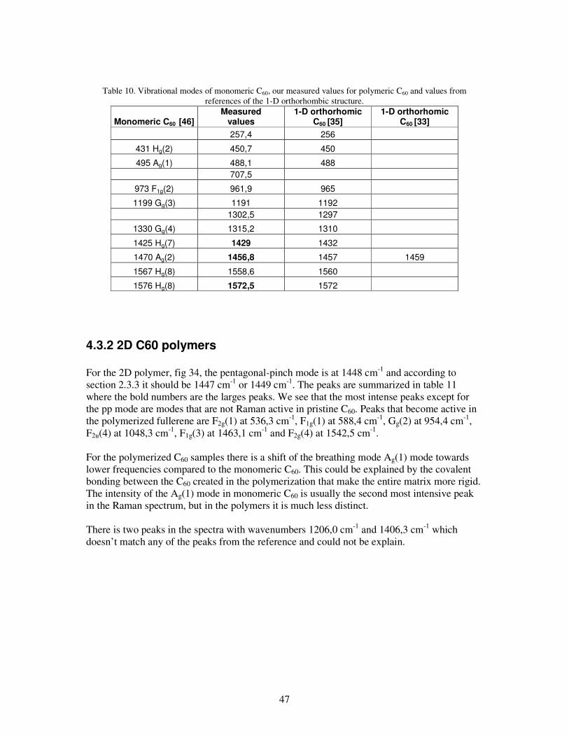
4.3 Raman study of polymerized fullerenes.......................................................................46 4.3.1 1D C60 polymers .................................................................................................46 4.3.2 2D C60 polymers .................................................................................................47

5 Summary..........................................................................................................................49 5.1 Summary ....................................................................................................................49 5.2 Conclusions ................................................................................................................49 5.3 Recommendations for future work ..............................................................................50 Extra................................................................................................................................50

Appendix A ..................................................................................................................55 Appendix B ..................................................................................................................58

4

1 Thesis introduction

1.1 Background The research on carbon based nanostructures has escalated in the last years. This is much due to the discovery of the single walled carbon nanotube (SWNT) by Iijima 1993, and the remarkable properties that the nanotubes have shown both in theory and in practice. The tubes can have either semiconducting or metallic electronic band structure, and they have outstanding mechanical properties. It has however shown to be difficult to construct materials using only nanotubes, due to their week van der Waal interactions. Work is being done trying to make nanotube composites, and by that transfer some of the remarkable properties of the SWNT to other materials. Today most of the research in on nanotube composites is done using polymeric matrixes because they are easier to handle than metals. Tests have shown that it is not possible just to mix raw nanotubes in the matrix and hope to get good results. The nanotubes interact badly with the matrix and have a tendency to agglomerate. To get the tubes to connect better with the polymer matrix, chemical groups that easier interact with the polymers are being attached to the nanotube sidewalls (functionalization). Fullerenes are another carbon nano material that has shown interesting properties. The fullerenes were discovered in 1985 by researchers at Rice University and named after Richard Buckminster Fuller and are sometimes called buckyballs. It has, among other things, shown possible to construct intrinsic materials from fullerenes with interesting properties. Of all methods used to characterize carbon nanostructures, Raman spectroscopy is the most powerful. The one dimensional structure of the CNTs create pikes in the electronic density of states, which gives rise to a resonance phenomenon that occurs when the tubes are lit up on with matching excitation energies, and results in a strong Raman signal. To investigate physical properties of carbon nanostructures, high pressure experiments have shown of interest. As an example, it has shown possible to polymerize fullerenes using combinations of high pressure and temperature.

1.2 Motivation The projects were developed by Professor Alexander Soldatov at Luleå University of Technology. These projects needed to be started, and they are a part of a program aimed at development of new methods to produce novel nanostructured functional materials formed by polymerization of both fullerenes and nanotubes at high pressures and basic research on the physical and chemical properties of the products. An essential piece of the work needed to be dedicated to setting up a new High-pressure spectroscopy laboratory in the department of physics. Professor Soldatov are having a research cooperation with a research team at Nancy University in France, and as the laboratory on LTU has new state of the art equipment, the lab crew on LTU can provide nice complimentary work to the research at Nancy University.

5

1.3 Thesis Outline This thesis begins with a short introduction which is followed by brief theory, experimental methods, results and discussion, and finally we round up with a summary

2 Theory

2.1 High pressure methods in materials synthesis High-pressure is an important parameter to probe physical properties and synthesis of new materials. To reach these pressures different techniques can be used. The major effects of high pressure on matter include decrease of volume, phase transitions, changes in electrical, optical, magnetic, and chemical properties, and increases in viscosity of liquids. In general solids are less compressible than liquids, and the compressibility of both solids and liquids decreases with increasing pressure [1]. There are two main techniques that are used in high pressure research, static and shock. Both techniques are capable of generating pressures in the megabar range, but in particular, static pressure yields continuous states on an isotherm (or isochore, when heating), with a slow loading rate, and sock compression can load samples to megabar pressures in a fraction of a nanosecond to microseconds. An example of a device used to generate high static pressure is a diamond anvil cell (see 2.1.1).

2.1.1 Diamond anvil cell (DAC)

A diamond anvil cell works much like a vice, squeezing the sample between two anvils, fig 1. To generate as high a pressure as possible, the anvils have to be made from the hardest material possible, diamonds. Another advantage in using diamonds as anvils is that they are transparent to a wide spectral range (visible, etc.), which makes it easier doing measurements on the sample. The sample is held at its place using a metal gasket as sample holder. The pressure that can be generated in a diamond anvil cell is limited to the size of the diamond through the force-area relation, and most of all to the strength of diamond as a material. One disadvantage of diamond anvil cells is that only small samples can be used. Another disadvantage in an ordinary dac is that the pressure is generated by manually tightening screws, making it hard to take small pressure steps. Pressures up to 3 Mbar can be reached with this method.

6

Fig 1, Schematic diagram of a diamond anvil cell (DAC). (A) Support, (B) screws, (C) diamond anvils, (D) gasket, (E) sample chamber. The principle of DAC operation: a) Diamonds (small top surface = culet) b) Gasket – sample chamber c) Pressure generation force application ( ~100kg - 300kg)

2.1.2 The gasket

The gasket is an important part of a high pressure experiment. The material and structure of the gasket may be freely chosen and might vary from one high-pressure experiment to another. A common choice of material that is used both in the range up to 10GPa is a hard-rolled austenitic stainless steel, (in the multi-mega bar range Rhenium is used). Materials that show little or none work-hardening, such as mild steel, should be avoided. The gasket is preferable thicker then you want to use in your experiment. This means that you can produce the exact thickness you need for your experiment by doing a pre-indent and you only have to have one kind of thickness of your gaskets in stock [2].

2.1.3 Pre-indentation of gasket

Pre-indentation has many advantages. Two of them are already mentioned in 2.1.2, but it also makes the loading process easier. If you don’t have a pre-indent, you face the problem of centering the gasket hole on the culets and loading the sample at the same time. With a pre-indent the centering of the hole is already taken care of due to that the position of the hole is already registered and well centred in the indent. It also makes it easier to choose the correct thickness of the gasket as you can follow the hole during your experiments, and depending on what happens make the gasket thinner or thicker the next time. The part of the gasket under the diamonds undergoes plastic deformation (and is extruded) as the anvils advance with increasing pressure. In the material, the hydrostatic pressure decreases linearly in the direction of the extrusion. The gradient of the pressure increases as the gasket becomes thinner. The extrusion of the material can go either outwards (extending the hole), inwards (collapsing the hole), or both outwards and inwards. If the extrusion is booth inwards and outwards there will be a segment of metal that does not move at all and separates the two moving segments. The choice of gasket thickness and the diameter of the hole depend on the pressure medium used. In the case of using the relatively incompressible alcohol or argon as media, the hole should be one-third to two-fifths of the culet diameter, since the hole is expected to shrink just

7

slightly during the experiment. If for example helium is used, which is much more compressible, the gasket hole is expected to shrink at about a factor of 2 or more. In this case the hole should be made larger. The primary symptom of gasket failure is if the hole starts to grow [3].

8

2.2 Physical properties of carbon-based nanostructured materials

Carbon is the only element in the periodic table that has isomers from 0 dimensions (0D) to three dimensions (3D), (the 0D C60 fullerene cluster, the 1D nanotube, the 2D graphite and the 3D diamond), see fig 2.

Fig 2, Isomers of carbon Carbon is the sixth element in the periodic table and is listed in top of column 4. Each carbon atom has six electrons which occupy 1s2, 2s2, and 2p2 atomic orbitals. The ground state of carbon is 3P (S=1, L=1). The 1s2 orbital contains two strongly bound core electrons and the 2s22p2 orbitals contain four more weakly bound valence electrons. In the crystalline phase, the valence electrons give rise to 2s, 2px, 2py, and 2pz orbitals which are important in forming covalent bonds in carbon materials. The energy difference between the upper 2p energy levels and the lower 2s level is small compared with the binding energy of the chemical bonds, and therefore the electronic wave functions for these four electrons will easily mix with each other and thereby changing the occupation of the orbitals so that the binding energy of the carbon atom and its neighbours will get enhanced. This mixing of orbitals is called hybridization [4].

2.2.1 Fullerenes

The C60 fullerene was discovered 1985 by H.Kroto, R.Curl, and R.Smalley [5], and they were rewarded in 1996 with the Nobel price in chemistry. They use a technique that involves vaporization of graphite by laser irradiation. The C60 molecule consists of 60 carbon atoms and has the shape of a regular truncated icosahedron belonging to the point group Ih, fig 3a. A fullerene is a closed cage molecule containing only hexagonal and pentagonal faces. By the ‘isolated pentagon rule’ all fullerenes must have 12 pentagonal faces and an arbitrary number of hexagonal faces. The smallest fullerene to satisfy this rule is the C60 and the second smallest is the C70. Each carbon atom is trigonally bonded to three other carbon atoms and there are two different types of bonds in the molecule. Two single C-C bonds are located along a pentagonal edge at the fusion of a hexagon and a pentagon and a third bond is located at the fusion between two

9

hexagons and is a double bond. The bond lengths for the single bonds are 1,46 Å and for the double bond is 1,40 Å [6]

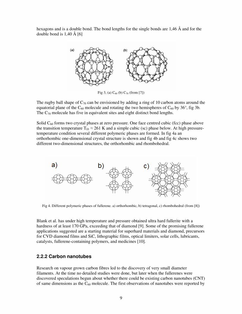
Fig 3, (a) C60 (b) C70 (from [7])

The rugby ball shape of C70 can be envisioned by adding a ring of 10 carbon atoms around the equatorial plane of the C60 molecule and rotating the two hemispheres of C60 by 36°, fig 3b. The C70 molecule has five in equivalent sites and eight distinct bond lengths. Solid C60 forms two crystal phases at zero pressure. One face centred cubic (fcc) phase above the transition temperature T01 ≈ 261 K and a simple cubic (sc) phase below. At high pressure-temperature condition several different polymeric phases are formed. In fig 4a an orthorhombic one-dimensional crystal structure is shown and fig 4b and fig 4c shows two different two-dimensional structures, the orthorhombic and rhombohedral.

Fig 4. Different polymeric phases of fullerene. a) orthorhombic, b) tetragonal, c) rhombohedral (from [8])

Blank et al. has under high temperature and pressure obtained ultra hard fullerite with a hardness of at least 170 GPa, exceeding that of diamond [9]. Some of the promising fullerene applications suggested are a starting material for superhard materials and diamond, precursors for CVD diamond films and SiC, lithographic films, optical limiters, solar cells, lubricants, catalysts, fullerene-containing polymers, and medicines [10].

2.2.2 Carbon nanotubes

Research on vapour grown carbon fibres led to the discovery of very small diameter filaments. At the time no detailed studies were done, but later when the fullerenes were discovered speculations begun about whether there could be existing carbon nanotubes (CNT) of same dimensions as the C60 molecule. The first observations of nanotubes were reported by

10

Iijima 1991, and were done by transition electron microscopy [11]. The single-walled carbon nanotubes (SWNT) were discovered in 1993 [12]. The CNT has a small enough diameter compared to its length to be a one dimensional object. A single-wall carbon nanotube can be described as a 2D graphene sheets rolled up into a seamless cylinder in which sp2 hybridization is present. Multi-walled carbon nanotubes (MWCNT) are built up from many single-wall nanotubes arranged layer by layer inside each other. The distance between the layers are approximately equal to the graphite inter-layer distance. The diameter range of the SWNT is about 0.7-10.0 nm, though most of them have a diameter less than 2 nm [4]. The system that is used to classify the different single wall nanotubes are based on the orientation of the hexagons that the carbon atoms are arranged into, see fig 5. The primary symmetry classification of the nanotubes is to see if the tube is chiral or achiral. The achiral class is then divided into two groups, armchair, zigzag, making it three sub-classes of single walled nanotubes. A nanotube is achiral if its mirror image has an identical structure as the original, and chiral if it is not. The chirality is described by the chirality vector, hC , and it can be expressed by the real

space unit vectors 1a and 2a of the hexagonal lattice, see equation 1 below and fig 5.

),(ˆˆ 21 mnamanCh ≡+= (n,m are integers, nm ≤≤0 ) (1)

The chirality angle θ denotes the angle in which the hexagons are tilting with respect to the direction of the nanotube axis. Because of the hexagonal symmetry θ can wary between 0° and 30° and is given by

+= −

mn

m

23

tan 1θ (2)

The diameter, dt, of the CNT is given by

ππ

223 mnmnaCd CCh

t

++== (3)

where aCC is the nearest-neighbour C–C distance (1.421 Å in graphite)

11

Fig. 5, The atomic configuration of a single layer of graphite known as a graphene sheet. The vectors are used when describing the formation of SWNT’s by rolling the graphene sheet into a seamless cylinder. C is the chiral vector, θ the chiral angle and a1, a2 the unit vectors of the graphene. T describes the smallest translation along the tube axis. In the case shown C represents a (5, 2) tube. In table 1 chiral index (n,m) and chiral angle (θ) of the different tube types are presented.

Table 1. Chiral index and angle for different types of tubes Tube type chiral index (n,m) chiral angle (θθθθ)

Armchair n , n 30o

Zigzag 0 , n 0o

Chiral n , m 0<θ<30o

The unit cell for a carbon nanotube in real space is given by the rectangle generated by the chiral vector Ch and the translational vector T, fig 5. There are 2N carbon atoms per unit cell (where N is the number of hexagons in the unit cell), which means there will bee N pairs of bonding π and anti-bonding π* electronic energy bands. Similarly the phonon dispersion relations will consist of 6N branches, resulting from a vector displacement of each carbon atom in the unit cell. The phonon dispersion relations of CNTs can be understood by zone folding the phonon dispersion curves for a single 2D graphene sheet [4]. Phonons denote the quantized normal mode vibrations that strongly affect many processes in condensed matter systems, including thermal, transport and mechanical properties. The electronic structure of a single wall carbon nanotube can to the first order be obtained from 2D graphite, but the quantum confinement of the 1D electronic states must be taken into account. The σ bands make up the covalent bonds within the 2D graphene sheets, while the π bands make up the weaker van der Waals interactions from one graphene sheet to another as in 3D graphite. The π bands are close to the Fermi level, giving the possibility for electrons to be exited from the valence band to the conduction band optically [13]. The electronic structure of most SWNTs can be obtained by using a nearest neighbour tight binding model [4], however if the diameter of the tubes is small, the curvature of the graphene sheet induces changes in the bound distance between the carbon atoms and causes mixing of the σ and π bounds. Thus more accurate methods must be used [14]. The 1D nature of the nanotube results in several spikes (van Hove singularities) in the electronic density of states (EDOS). The sub band peak positions of the EDOS are unique for

12

every diameter and chirality of the carbon nanotubes [15]. Plotting the energies between the van Hove singularities, fig 6, against the diameter of the tubes will result in a so called Kataura plot fig 7. From the Kataura plot it can be determined which tubes that are possible to detect with a specific excitation source. When the laser excitation energy matches the energies of the van Hove singularities, the tubes are in resonance. The SWNTs can show either metallic or semiconducting behaviour. Approximately one third of all nanotubes are metallic and two thirds are semiconducting. A general rule to determine if a tube is metallic or semiconducting is to look at its chiral index. If (2n + m), or equivalently (n - m), is a multiple of 3, then the tube is metallic and if not, the tube is semiconducting. The armchair nanotube, who has a chiral index of (n , n), is always metallic [4].

Fig 6. Band structure and density of states of a

semiconducting zigzag nanotube. The Fermi level is set to zero.

(Thomsen & Reich)

Fig 7. Kataura plot: transition energies of

semiconducting (filled symbols) and metallic (open) nanotubes as a function of tube

diameter. Calculated from the van-Hove singularities in the joint density of states within the third-order tight-binding approximation (Tomsen &

Reich)

Carbon nanotubes exhibit outstanding physical properties: Single walled carbon nanotubes are predicted to show ballistic conductive behaviour with a resistance as low as 6454 Ω/tube, independent of the tube length. This would correspond to a bulk resistivity several times lower than copper [16]. Individual nanotubes has shown resistivities in the range of 5.1*10-6–5.8Ωcm. The carbon-carbon chemical bound in a graphene layer is probably the strongest chemical bound known in nature. Depending on the quality of the sample, the Young modulus of SWNTs has been measured to be over 1 TPa, which is larger that that of any other known material [17]. The thermal conductivity can be as high as 3500 Wm-1K-1 at room temperature for a single CNT, and they also have a very tiny expansion coefficient due to the strong in-plane C–C bonds [18]. For comparison, copper and silver, which have the highest electrical conductivities of any metal, have thermal conductivities of just around 400 Wm-1K−1 at room temperature. [19]

13

Due to their unique properties, the CNT have great prospective for applications in various disciplines. Application areas cover very widely for field emitters, hydrogen storage, transistor, secondary battery, supercapacitor, fuel cell, gas sensor, composites, and nanoprobes [15]. The MWCNT does not show quite as good physical properties as the SWCNT, but they are much cheaper to produce which makes them suitable for design of inexpensive CNT-based materials, for example composites. The smallest in the family multi-wall nanotubes is the double-wall nanotube which is built up from two single wall nanotubes. The walls of the nanotubes are rarely perfect. Defects in form of pentagons, heptagons or even vacancies can easily be created instead of hexagons. Local and global curvature, inter-tube and inter-shell interactions are dramatically modifying the electronic properties from those obtained from simple zone folding [4] of the graphene band structure. These imperfections give rise to the disorder induced D-band in Raman spectroscopy, se sec 2.3.3. However the possibility to control these defects will probably be important in future tailoring of carbon nanotube properties. Single-walled carbon nanotubes are rarely found as isolated specimens. They often assemble in bundles to minimize their energy through van der Waals interactions. The diameters of the nanotubes in a bundle are rather homogenous, but they often have a wide distribution of chiral angels. The present technologies for CNT synthesis always produce samples with mixing chiralities.

2.2.3 CNT-based composite materials

The electrical, mechanical and thermal properties of an individual single wall carbon nanotube make them very attractive in materials design. SWNTs interact with each other only through week van der Waal interactions, which makes a strong material that is built up only from the nanotubes themselves difficult to create. Many research groups are trying today to make composites containing nanotubes, and there by enhance the properties of the matrix material. As an example, estimations are done that show that in a copper-nanotube composite, the resistivity could be as low as 50% lower then in copper [16]. Research on CNT-reinforced nanocomposits is showing exiting and promising results. Polymers, ceramics and metals are being tested as matrix material, but the most studies has been done on the CNT-polymer composites due to their relatively convenient processibility. Both MWCNTs and SWCNTs have been used, but SWCNTs are usually favoured over MWCNTs as structural reinforcements due to their physical properties. Nevertheless the CNT composites still lag quite far behind in comparison to single (individual) nanotubes in terms of physical properties. The main problems in the making of nanotube composites are how to evenly disperse the tubes in the matrix and to get the nanotubes to interact with the matrix. Some remarkable results from experiments on CNT-nanocomposites:

14

• 80% improvement in the tensile modulus for polyvinyl alcohol (PVA) by adding 1 wt% MWCNTs [20]

• an increase of about 140% in ductility for ultrahigh molecular weight polyethylene

adding 1 wt% of MWCNTs [21]

• By dispersing 2 wt% MWCNTs in Nylon-6, Liu et al showed that the elastic modulus and the yield strength of the composite were increased by 214% and 162%, respectively [22]

• a three fold increase in youngs modulus is achieved adding 1 wt% SWCNT to

polypropylene [23]

15

2.3 Synthesis and Characterization of carbon-based nanostructured materials When fullerenes were discovered a laser ablation method was used for their production. This method generated only small quantities of fullerenes but the discovery of an arc discharge method in 1990 made it possible to produce larger quantities [7]. These methods produce carbon “soot” from which the fullerenes are extracted by use of appropriate solvents [24]. The techniques for production of CNTs can be divided into three main categories:

• Laser ablation • Arc-discharge • Chemical Vapour Decomposition (CVD)

In all these synthesis methods, metals are used as process catalysts. Often used metals are iron, cobalt, nickel and yttrium. The metal catalysts favour the growth of SWNTs. In the case of the arc-discharge method, the metals are mixed with solid pure carbon electrodes. In the laser ablation process, the metal is placed on the substrate forming nanoclusters. In the CVD method the metal forms gaseous clusters acting as nuclei for the SWNT synthesis. One of the most commonly used CVD processes is the high-pressure CO conversion (HiPCO) process where SWNTs with up to 97% purity are produced by flowing CO and Fe(CO)5 under high pressure (30–50 atm). Nanotubes with diameters as low as 0,7 nm can be created with this process, which is the lowest diameter expected for SWNTs. The average diameter produced by this method is 1,1 nm. [25] There are numerous techniques used to characterize carbon based nanostructures:

• X-ray photoelectron spectroscopy (XPS) (allows determining the functionalization of the nanotubes).

• Scanning tunnelling microscopy (STM) is a powerful technique used to obtain three

dimensional images and electronic structure of the nanotubes. The helicities of the nanotubes can be determined with high resolution images.

• Neutron diffraction is widely used for determination of structural features such as

bond length and possible distortion of hexagonal network.

• X-ray diffraction (XRD) is used to obtain some information on the interlayer spacing, the structural strain and the impurities.

• Transmission electron microscopy (TEM) is used to investigate structural details such

as intershell spacing, chiral indices, and helicity.

• Infrared spectroscopy is often used to determine impurities remaining from synthesis or molecules capped on the nanotube surface.

16

• Photoluminescence technique can be used to determine geometries and diameters of CNTs. In order to observe the photoluminescence phenomenon, the bundles must be separated into individual tubes.

• Raman spectroscopy is the most powerful technique to characterize carbon nanotubes.

Without sample preparation, a fast and non-destructive analysis is possible. Moreover, Raman spectra simulations are performed on various nanotubes geometries.

For a correct characterization of nanotubes, all these techniques described here can not be used separately but must be used in complementary ways [26].

2.3.1 Polymerization of fullerenes at high pressure C60 can be polymerized by submitting the material either to ultraviolet or visible light, photo polymerisation, or to high pressures and high temperatures. Photo polymerisation can only be carried out on very thin films. In high pressure- high temperature polymerisation larger volume samples of polymerized material can be produced. In the polymeric phases, the weak van der Waals binding between molecules is replaced by covalent bonds via a 2 + 2 cycloaddition reaction [27]. In this reaction the double bonds forming borders between hexagons open up to form the intermolecular bonds, fig 4 in section 2.2.1.

Fig 8. Pressure-temperature phase diagram of C60 (from [33])

Depending on the exact temperature-pressure conditions, one-dimensional (1D), two-dimensional (2D) and tree-dimensional (3D) polymerisation have been found [28]. In the 1D phase the C60 molecules forms linear chains in an orthorhombic crystal structure. As an initial intermediate in the formation of the linear chains the formation of the dimer C120 and higher oligomers has been observed. There are two different structures in the 2D phase, tetragonal and rhombohedral see fig 8. In the 2D polymers the C60 molecules are linked via covalent bonds in the planes while interaction between the planes is van der Waals.

17

2.3.2 Functionalization of carbon nanotubes

As already mentioned, carbon nanotubes exhibit extraordinary properties, and in order to transfer these properties in to composite materials functionalization has been proposed as a first step. The main reasons to use functionalized tubes are that they have shown to be easier to disperse, and they interact better within a composite matrix. Other areas in which functionalized nanotubes can be useful are in electronic applications and sensing applications [29]. There are three main strategies that can be used when functionalizing nanotubes. One strategy is to functionalize from created defects, another to functionalize the end caps of carbon nanotubes, and one is to functionalize the sidewalls of the tube, see fig 9 [30]. Of these strategies, the most interesting in order to get the nanotubes to interact with composite matrixes is the sidewall functionalization due to the increased solubility of the SWNTs, which allows for better manipulation and processing, and increased solubility leads to better dispersion in polymeric systems. There are two categories of side wall functionalization technique, depending on the type of bond binding the functional group to the nanotube. The two possible cases are either a covalent bond or a van der Waals bond. One big advantage of covalent functionalization is that no surfactant that can affect the properties of the composite has to be used, since such additives are difficult to remove and thus may have negative effects on the properties of the composites [31]. Covalent sidewall functionalization can even be performed selectively (i.e. metallic nanotube can be modified without affecting the semiconducting tubes) [32]. Another interesting property of functionalization is that the surface tension of the tubes can be modified. The pristine nanotubes are hydrophobic in nature due to their van der Waals interaction. Functionalization leads to transform the hydrophobic surface to hydrophilic one by ionizing the CNT surface [15]. (One of the most common van der Waal functionalizations is by use of Sodium dodecyl sulphate (SDS) in attempts to disperse nanotubes.)

Fig. 9, Example on sidewall covalent functionalization

To analyse the functionalized nanotubes, the following techniques are the most commonly used: Absorption and resonance Raman spectroscopy are employed to ensure that the functionalization is covalent and occurs at the side-walls. Once covalent side-wall functionalization is confirmed, thermal gravimetric analysis (TGA) and x-ray photoelectron spectroscopy (XPS) are used to determine the degree of functionalization. (Imaging techniques such as atomic force microscopy (AFM) scanning electron microscope (SEM), and transmission electron microscopy (TEM) are also used as a compliment.) [30]

18

2.3.3. Vibrational properties of carbon nanostructures from Raman spectroscopy

Fullerenes The vibrational modes of C60 fullerene can be subdivided into two classes: intermolecular vibrations (or lattice modes) and intramolecular vibrations (or simply ‘molecular’ modes). C60 intramolecular modes The first-order Raman and infrared spectra of the C60 molecule are among the simplest compared to other fullerene molecules. This is because of the high symmetry of the molecule. Starting with 180 total degrees of freedom and subtracting tree corresponding to translation and tree corresponding to rotations, yields 174 vibrational degrees of freedom for an isolated C60 molecule. From group theory the 174 vibrational degrees of freedom corresponds to 46 distinct intramolecular modes. Of the 46 modes, ten are Raman-active (2Ag + 8Hg) in first order, four are infrared (IR)-active (4F1u) and the remaining are optically silent. The two Ag modes are nondegenerate and the eight Hg are fivefold degenerate. In the Ag(1) ‘breathing’ mode (492 cm-1) all the 60 carbon atoms are involved in identical radial displacement. The Ag(2) mode (1468 cm-1) is called the ‘pentagonal pinch mode’ and it involves tangential displacement with a contraction or expansion of the pentagonal rings. The eight Hg modes are more complex and span the wavenumber range from 269 Hg(1) to 1575 cm-1 Hg(8) [7]. There is a tendency of the lower frequency molecular modes (ω < 700 cm-1) to have displacements that are more radial in character and the high-wavenumber (ω > 700 cm-1) modes tend to exhibit approximately tangential displacement. The C60 solid has vibrational frequencies similar to those for a free molecule because of the very weak van der Waals bonding between the molecules. The expected number of second-order Raman lines are consider to be very large because it include both overtones and combination modes of the first order modes. From group theoretical considerations we get a total of 151 modes with Ag symmetry and 661 modes with Hg symmetry. The study of the second-order Raman spectra of C60 is a powerful technique for the determination of the frequencies of the 32 silent first order modes [7].

C60 intermolecular modes In the solid phase of C60 there is an orientational ordering temperature at T01 ≈ 261 K. At temperatures well below the orientional ordering temperature there are five additional modes that are Raman-active, but observation by Raman spectroscopy is difficult because of their low wavenumbers ( < 60 cm-1). Above the orientational ordering temperature the C60 molecules rotate rapidly about their equilibrium positions in the fcc lattice and thus no rotational intermolecular modes exist.

19

Polymerisation of C60 After polymerisation of C60 most of the Hg modes split into several components and new modes appear which were optically silent earlier. This is due to change in symmetry. A useful method to identify the polymeric structure of C60 by Raman spectroscopy is to follow the evolution of the pentagonal pinch mode. This is because the number of double bonds forming borders between hexagons will decrease as the bonds break up to form the intermolecular bonds which leads to lower intramolecular average bond stiffness. The pentagonal pinch mode has been found to shift to 1464 cm-1 for dimers, to 1459 cm-1 for linear chains, and to 1447 cm-1 for tetragonal polymers [33]. For the rhombohedral it shifts to 1410 cm-1[34]. Other values of the shift of the pp mode were found to be 1462 cm-1 for dimers, 1457 cm-1 for linear chains, 1449 cm-1 for tetragonal and 1406 cm-1 for rhombohedral polymers [35]. Another sign of polymerisation is the appearance new peaks in the intermolecular vibration region between 50 and 200 cm-1. In ref [36] three well-resolved Raman peaks at 97, 119 and 173 cm-1 was found and in ref [37] four peaks was found at 98, 121, 157, and 174 cm-1. Single-wall carbon nanotubes

First-order Raman scattering in the RBM and G-band of SWNTs In the Raman spectra of SWNTs the strongest features of the first-order scattering processes are the radial breathing mode RBM and the tangential G-band, see fig 20 and 22 in section 4.2.1. The RBM correspond to vibration of the carbon atoms in the radial direction, like the tube were breathing. Typically it is observed in a frequency range of about 100-500 cm-1 and its appearance is a strong evidence of SWNT presence in the sample [13]. In CNT samples containing isolated SWNT it is possible to find only one RBM. In samples containing bundles, all the tubes in resonance will be contributing to the spectra. The RBM frequency (ωRBM) is inversely proportional to the tube diameter and for characterization of the diameter (dt) distribution in a sample the following expression can be used:

21 C

d

C

t

RBM +=ω (4)

where C1 and C2 are parameters to be determined experimentally. Their dependence comes from the fact that the mass of all the carbon atoms along the circumferential direction is proportional to the diameter. Several values for the parameters have been proposed depending on CNT environment and tube-tube interactions. For SWNT in bundles values of C1=224 cm-1 and C2=14 [38] and for isolated SWNTs on a SiO2 substrate C1=248 and C2=0 [39]. For small diameter tubes dt < 1 nm the simple relation in equation 4 is not expected to hold exactly, due to nanotubes lattice distortions. In order to get a good characterization of the diameter distribution several laser excitation energies are needed. This is due to the different resonance energies of nanotubes with different diameters. From RBM measurements using several laser energies the ratio of metallic to semiconducting tubes in the sample can be estimated.

20

In graphite the peak at 1582 cm-1 is called the G-band, and is related to the tangential mode vibrations of the carbon atoms in a graphite plane. The corresponding mode in SWNTs is composed of several peaks. The two main peaks are the G+ at 1590 cm-1, which is associated with vibrations along the nanotubes axis, and G- at 1570 cm-1, which associated with vibrations along the circumferential of the tube. The frequency of the G+ is sensitive to charge transfer from dopant addition [13]. The shape of the G- is dependent on whether the SWNTs are metallic or semiconducting. For metallic tubes it has a Breit-Wigner-Fano (BWF) lineshape and for semiconducting it has a Lorentzian shape. The BWF is described by

( )[ ]( )[ ]2

2

0/1

/1)(

Γ−+

Γ−+=

BWF

BWF qII

ωω

ωωω (5)

where the 1/q represents the asymmetry of the peak shape, BWFω , 0I and Γ are fitting parameters of the central frequency, the intensity and the broadening factor, respectively. The big difference in the G- profile for metallic and semiconducting nanotubes is useful for determine the specific type of CNT that is present in the sample. Charge transfer to SWNTs can lead to an intensity increase or decrease of the BWF feature. Second-order Raman scattering, D- and G’-band of SWNTs In difference to the first-order features the second-order phonon mode frequencies show dispersive behaviour, i.e. change with laser excitation wavelength. The two main peaks that shows this behaviour are the D-band at 1350 cm-1 and the G’-band occurring at 2700 cm-1 (~2 ωD) for a laser excitation of 2,41 eV. The D-band stemming from the disorder-induced mode in graphite with the same name and the G’ is its second harmonic. The D-band frequency changes by 53 cm-1 when changing the laser energy by 1 eV [13]. See fig 20 and fig 22 in section 4.2.1 for examples of the dispersive behaviour of the D-band. Analysis of the intensity of the D-band can be used to identify structural modifications or defects on the nanotube sidewalls and the intensity ratio D/G can determine sample purity. With covalent sidewall functionalization an increased in D-band intensity are expected [29].

Raman spectra of MWNTs Because of the large distribution of diameters from small to very large in the MWNTs most features from the SWNT spectra are missing. The RBM signal from large tubes is usually too weak and the RBM can only be observed in some cases for small diameter inner tube (less than 2 nm) when good resonance condition is established because of the broadening of the signal. The splitting of the G-band is small in MWNTs and appears as one weakly asymmetric peak close to the graphite frequency of 1582 cm-1.

21

3 Experimental methods

3.1 High-pressure method

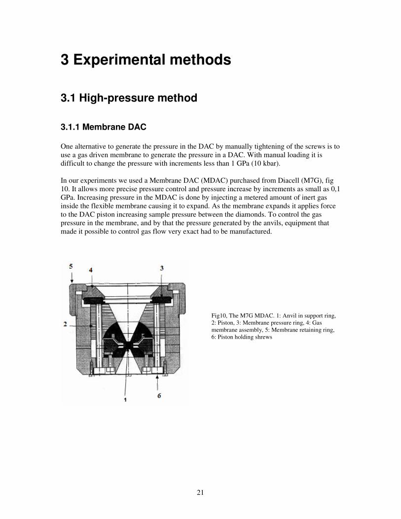
3.1.1 Membrane DAC

One alternative to generate the pressure in the DAC by manually tightening of the screws is to use a gas driven membrane to generate the pressure in a DAC. With manual loading it is difficult to change the pressure with increments less than 1 GPa (10 kbar). In our experiments we used a Membrane DAC (MDAC) purchased from Diacell (M7G), fig 10. It allows more precise pressure control and pressure increase by increments as small as 0,1 GPa. Increasing pressure in the MDAC is done by injecting a metered amount of inert gas inside the flexible membrane causing it to expand. As the membrane expands it applies force to the DAC piston increasing sample pressure between the diamonds. To control the gas pressure in the membrane, and by that the pressure generated by the anvils, equipment that made it possible to control gas flow very exact had to be manufactured.

Fig10, The M7G MDAC. 1: Anvil in support ring, 2: Piston, 3: Membrane pressure ring, 4: Gas membrane assembly, 5: Membrane retaining ring, 6: Piston holding shrews

22

3.1.2 Pressure control box

In order to be able to do fine tuning and control of the gas pressure in the membrane we designed a gas loading system (pressure control box), fig 11.

Fig 11, Pressure Control box scheme. List of components: 1: Fine tuning needle valve, 2: Bleed Valve, 3: Regular ball valves, 4: Quarter turn valve, 5: 0,5 µm sintered filter, 6: Pressure indicator. The work principle of the box is easy. First gas is let in to the ballast volume from the small bottle. Now the fine tuning valve (1) is opened slightly to pressurize the system. When a desired pressure is reached, the quarter turn valve can be shut, the pressure released in the box and the capillary tube disconnected from the box while pressure is maintained in the DAC. This system has many special features and allows for: a: Precise monitoring and control of gas pressure on the membrane

The digital manometer “LEO2” manufactured by Keller is used to measure the pressure in the box with a resolution of 100 mbar. The accuracy of LEO2 is 0,1%.

b: Fine tuning of pressure in the loading system

The fine tuning needle valve (1) allows us to control the gas flow from the ballast volume very precise. A Cv at 0,0005 corresponds to a gas flow of 20 l/min at a pressure difference of 200 bar, our design manages this easily

c: Cleaning of the gas before filling up the capillary A filter (5) with a pore size of 0,5 mm cleans the gas before the gas reaches the capillary tube.

d: Evacuation for use of special gases

23

The system can be evacuated and the grade of the vacuum can be measured close to the capillary tube. The small bottle makes the box easy to handle, and there is a possibility to refill the bottle with other gases if needed.

e: Disconnection of the DAC with maintained pressure

The use of miniature quick-connectors and a quarter turn valve on the capillary tube, makes it possible to seal of the DAC from the rest of the system and disconnect the DAC with maintained pressure.

f: High safety of diamonds

The small ballast volume makes it impossible to raise the pressure in the system to a higher pressure than 40 bars in one step. The possibility to seal the DAC out from the high pressure box with a quarter turn valve if something looks suspicious. The long capillary tube prevents the pressure to rise quickly on the membrane.

24

3.2 Sample preparation

3.2.1 Preparation of sample holders and sample loading in a DAC

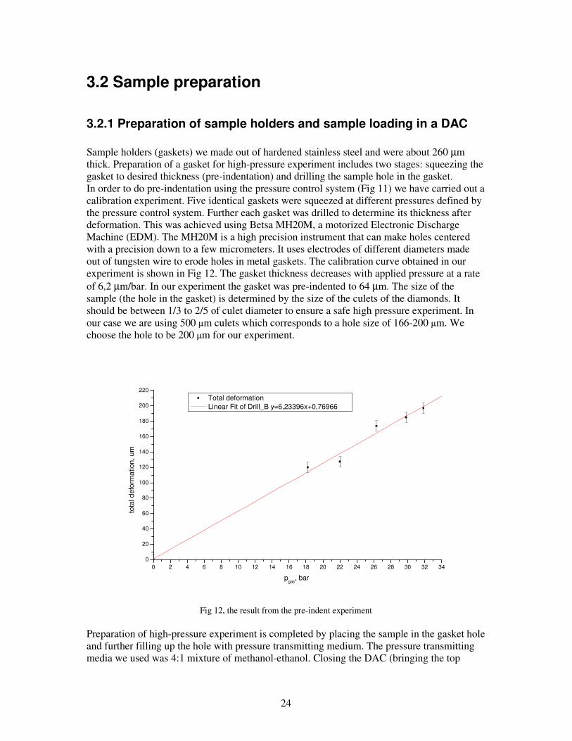
Sample holders (gaskets) we made out of hardened stainless steel and were about 260 µm thick. Preparation of a gasket for high-pressure experiment includes two stages: squeezing the gasket to desired thickness (pre-indentation) and drilling the sample hole in the gasket. In order to do pre-indentation using the pressure control system (Fig 11) we have carried out a calibration experiment. Five identical gaskets were squeezed at different pressures defined by the pressure control system. Further each gasket was drilled to determine its thickness after deformation. This was achieved using Betsa MH20M, a motorized Electronic Discharge Machine (EDM). The MH20M is a high precision instrument that can make holes centered with a precision down to a few micrometers. It uses electrodes of different diameters made out of tungsten wire to erode holes in metal gaskets. The calibration curve obtained in our experiment is shown in Fig 12. The gasket thickness decreases with applied pressure at a rate of 6,2 µm/bar. In our experiment the gasket was pre-indented to 64 µm. The size of the sample (the hole in the gasket) is determined by the size of the culets of the diamonds. It should be between 1/3 to 2/5 of culet diameter to ensure a safe high pressure experiment. In our case we are using 500 µm culets which corresponds to a hole size of 166-200 µm. We choose the hole to be 200 µm for our experiment.

0 2 4 6 8 10 12 14 16 18 20 22 24 26 28 30 32 34

0

20

40

60

80

100

120

140

160

180

200

220

tota

l d

efo

rma

tion

, u

m

pgas

, bar

Total deformation

Linear Fit of Drill_B y=6,23396x+0,76966

Fig 12, the result from the pre-indent experiment

Preparation of high-pressure experiment is completed by placing the sample in the gasket hole and further filling up the hole with pressure transmitting medium. The pressure transmitting media we used was 4:1 mixture of methanol-ethanol. Closing the DAC (bringing the top

25

diamond in contact with the gasket) was monitored using material research microscope Olympus BX51. We performed 2 experiments with similar experimental methods. The first one with a 77 mm gasket, and the second done with a 63 mm gasket. The dac was placed under CRM-200 and connected to the pressure box through the capillary tube. A fast scan was made of the area to se precisely where the ruby crystals were located, (fig 14b). Spectra were acquired from all crystals once again to have as reference in methanol-ethanol mixture, see section 4.1.

3.2.2 Carbon nano materials

a) CNT functionalization

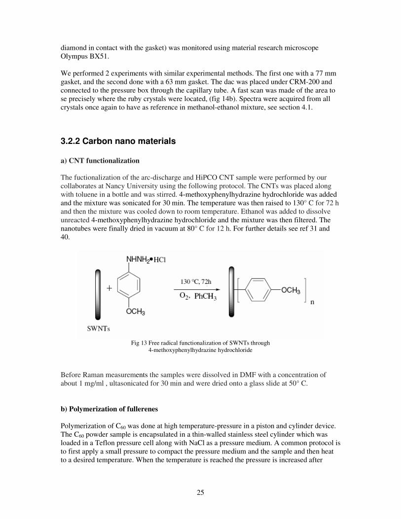
The fuctionalization of the arc-discharge and HiPCO CNT sample were performed by our collaborates at Nancy University using the following protocol. The CNTs was placed along with toluene in a bottle and was stirred. 4-methoxyphenylhydrazine hydrochloride was added and the mixture was sonicated for 30 min. The temperature was then raised to 130° C for 72 h and then the mixture was cooled down to room temperature. Ethanol was added to dissolve unreacted 4-methoxyphenylhydrazine hydrochloride and the mixture was then filtered. The nanotubes were finally dried in vacuum at 80° C for 12 h. For further details see ref 31 and 40.

Fig 13 Free radical functionalization of SWNTs through

4-methoxyphenylhydrazine hydrochloride Before Raman measurements the samples were dissolved in DMF with a concentration of about 1 mg/ml , ultasonicated for 30 min and were dried onto a glass slide at 50° C. b) Polymerization of fullerenes

Polymerization of C60 was done at high temperature-pressure in a piston and cylinder device. The C60 powder sample is encapsulated in a thin-walled stainless steel cylinder which was loaded in a Teflon pressure cell along with NaCl as a pressure medium. A common protocol is to first apply a small pressure to compact the pressure medium and the sample and then heat to a desired temperature. When the temperature is reached the pressure is increased after

26

which temperature and pressure is held constant for a certain time. Then the heat is switched of and the sample is cooled to room temperature before pressure is lowered to atmospheric. In the polymerization of fullerenes to 1D state NaCl was used as a semi hydrostatic pressure medium. The sample was heated to 550- 585 K and with a pressure of 1, 1 GPa [36]. To obtain the 2D polymerized sample the pristine material was subjected to a temperature of 820 K and pressure of 2,3-2,5 GPa [41].

27

3.3 Spectroscopic characterization

3.3.1 CRM-200

The Confocal Raman Microscope (CRM-200) combines a triple grating Raman spectrometer with a confocal optical microscope. With this combination it is possible to obtain a Raman spectrum of points of the sample with a lateral resolution in the sub-micrometer regime. For example using green excitation light, a resolution down to 220 nm is possible. The microscope, as well as the spectrometer and detectors, are optimized for the highest throughput and efficiency which gives the CRM-200 an unrivalled sensitivity. The system is equipped with two detectors: CCD and ADP The charge-coupled device (CCD) used is a 1D enhanced- back illuminated CCD detector that is cooled down to about -94 degrees Celsius. The SPCM-AQR Avalanche Photodiode detector (APD) is a self-contained module which has a single photon sensitivity over a spectral range from 400 nm to 1060 nm. With the CRM-200, a variety of Raman modes are possible: Single spectrum (Collection of Raman spectrum at selected sample area). Raman fast imaging (The ADP counts photons with a certain wavelength, creating a map of the intensities in the scan area) Time Spectrum (Collection of time series of Raman spectra at selected sample area) Line spectrum (Collection of Raman spectra along a selected line) Raman spectral imaging (Spectra collected from each point in a scan area) The most powerful mode of the CRM-200 is the Raman spectral imaging mode. Complete spectra are obtained at every image pixel. The number of pixels in the image is only limited by the computer memory. As an example, an image size of 512*512 would render in 262144 spectra acquired. Images can then be calculated from the spectra by applying large numbers of analyzing modes, like integrating over certain areas, calculating the peak position or peak width in the spectra. The distribution of different materials or properties of the sample can be analyzed in 3D and with spatial resolution down to 200 nm.

3.3.2 Ruby fluorescence

Ruby is a Al2O3 crystal containing about 5% Cr3+ ions. It can be found in nature (gems) and can be grown in a lab (synthetic ruby). The red colour comes from the presence of theCr3+ ions. Among the natural gems only diamond is harder. When lit upon with visible light, ruby emits light with certain wavelengths (fluorescence). Two prominent fluorescence peaks (R1 and R2) are centred around 694,2 nm and 692,8 nm respectively. These peaks are due to the 2E 4A2 transitions of Cr3+. The R1 and R2 lines exhibit a “red” shift when the ruby crystal is subjected to high pressure. This is due to the decrease of the energy gap between these two

28

states [42]. Pressure dependence of R1 and R2 wavelength is used to determine pressure in high-pressure experiments.

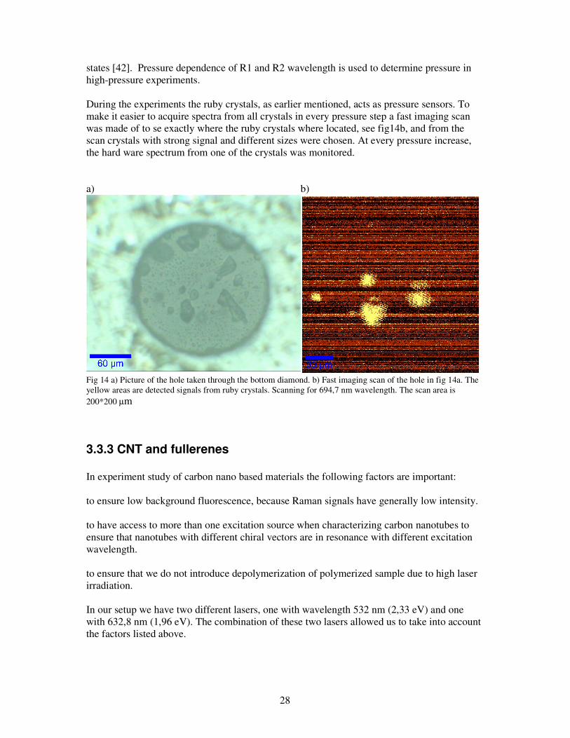
During the experiments the ruby crystals, as earlier mentioned, acts as pressure sensors. To make it easier to acquire spectra from all crystals in every pressure step a fast imaging scan was made of to se exactly where the ruby crystals where located, see fig14b, and from the scan crystals with strong signal and different sizes were chosen. At every pressure increase, the hard ware spectrum from one of the crystals was monitored. a)

b)

Fig 14 a) Picture of the hole taken through the bottom diamond. b) Fast imaging scan of the hole in fig 14a. The yellow areas are detected signals from ruby crystals. Scanning for 694,7 nm wavelength. The scan area is 200*200 µm

3.3.3 CNT and fullerenes

In experiment study of carbon nano based materials the following factors are important: to ensure low background fluorescence, because Raman signals have generally low intensity. to have access to more than one excitation source when characterizing carbon nanotubes to ensure that nanotubes with different chiral vectors are in resonance with different excitation wavelength. to ensure that we do not introduce depolymerization of polymerized sample due to high laser irradiation. In our setup we have two different lasers, one with wavelength 532 nm (2,33 eV) and one with 632,8 nm (1,96 eV). The combination of these two lasers allowed us to take into account the factors listed above.

29

4 Results and Discussion

4.1 Ruby fluorescence: calibration of DAC gas loading system

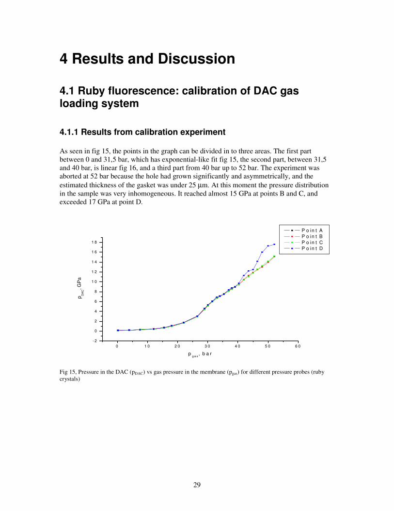
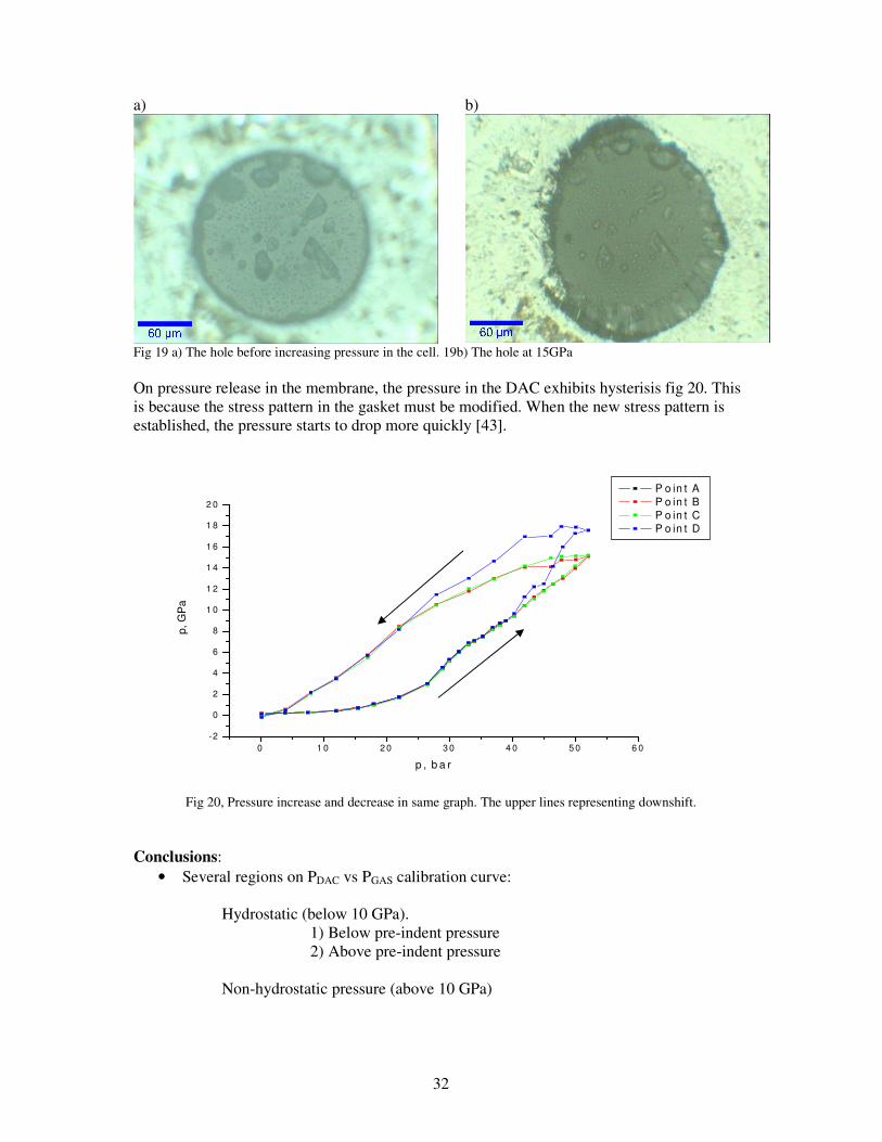
4.1.1 Results from calibration experiment As seen in fig 15, the points in the graph can be divided in to three areas. The first part between 0 and 31,5 bar, which has exponential-like fit fig 15, the second part, between 31,5 and 40 bar, is linear fig 16, and a third part from 40 bar up to 52 bar. The experiment was aborted at 52 bar because the hole had grown significantly and asymmetrically, and the estimated thickness of the gasket was under 25 µm. At this moment the pressure distribution in the sample was very inhomogeneous. It reached almost 15 GPa at points B and C, and exceeded 17 GPa at point D.

0 1 0 2 0 3 0 4 0 5 0 6 0

- 2

0

2

4

6

8

1 0

1 2

1 4

1 6

1 8

pD

AC, G

Pa

pg a s

, b a r

P o in t A

P o in t B

P o in t C

P o in t D

Fig 15, Pressure in the DAC (pDAC) vs gas pressure in the membrane (pgas) for different pressure probes (ruby crystals)

30

0 5 1 0 1 5 2 0 2 5 3 0

0

1

2

3

4

5

6

pD

AC, G

Pa

pg a s

, b a r

y = 0 ,0 0 5 6 8 1 * e x p (x /6 ,6 8 3 9 7 ) B

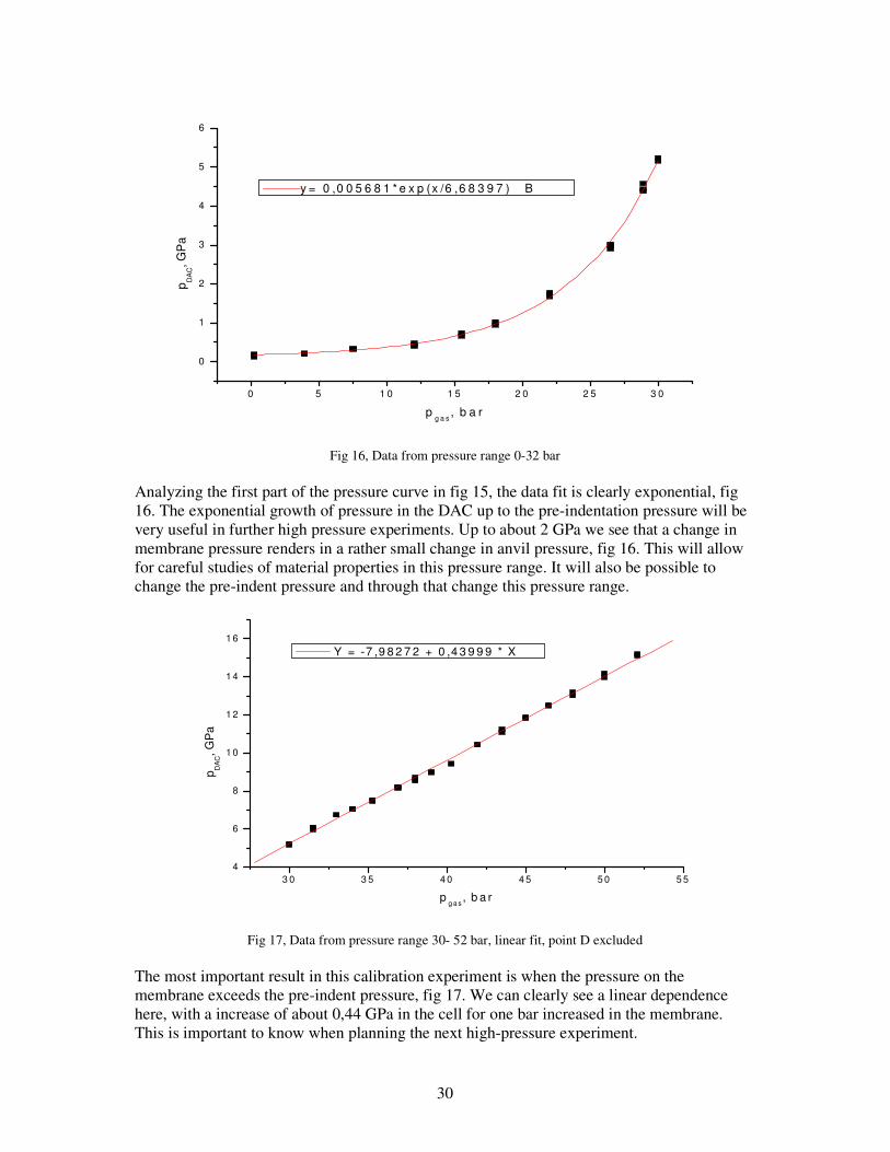
Fig 16, Data from pressure range 0-32 bar

Analyzing the first part of the pressure curve in fig 15, the data fit is clearly exponential, fig 16. The exponential growth of pressure in the DAC up to the pre-indentation pressure will be very useful in further high pressure experiments. Up to about 2 GPa we see that a change in membrane pressure renders in a rather small change in anvil pressure, fig 16. This will allow for careful studies of material properties in this pressure range. It will also be possible to change the pre-indent pressure and through that change this pressure range.

3 0 3 5 4 0 4 5 5 0 5 5

4

6

8

1 0

1 2

1 4

1 6

pD

AC, G

Pa

pg a s

, b a r

Y = -7 ,9 8 2 7 2 + 0 ,4 3 9 9 9 * X

Fig 17, Data from pressure range 30- 52 bar, linear fit, point D excluded

The most important result in this calibration experiment is when the pressure on the membrane exceeds the pre-indent pressure, fig 17. We can clearly see a linear dependence here, with a increase of about 0,44 GPa in the cell for one bar increased in the membrane. This is important to know when planning the next high-pressure experiment.

31

In the third part, between 40 and 52 bar, the pressure in the DAC exceeds 10 GPa. At this pressure, the methanol-ethanol mixture starts to transfer in to solid state, and the pressure will become non-hydrostatic. This explains why crystal D behaves differently from the other ruby crystals in this pressure area. Thus we can assume that crystallization of the pressure medium began in the middle of the sample as crystal D is the one that lie in the very middle of the sample hole. Generally over the experiment, as the pressure went up, the ruby peaks become less intense. Exceeding 10 GPa, the peaks start to broaden and get more defuse. This is due to the non-hydrostatic pressure as the solid state transfer of the methanol-ethanol mixture occurs, fig 18.

6 8 0 6 8 5 6 9 0 6 9 5 7 0 0 7 0 5 7 1 0

- 2 0 0

0

2 0 0

4 0 0

6 0 0

8 0 0

1 0 0 0

1 2 0 0

1 4 0 0

1 6 0 0

CC

D c

ts

W a v e le n g th ( n m )

0 G P a

9 G P a

1 6 G P a

Fig 18, Ruby fluorescence lines from crystal D, (left = 0 GPa, middle = 9 GPa, right = 16 GPa)

In the beginning of the experiment the hole had a diameter of 198 µm, fig 19a. Up to 31,5 bar the hole shrunk down to a diameter of 179 µm. Going above 31,5 bar in pressure on the membrane, the hole started to grow again, and more alarming it started to deform un evenly and move to the left. At 52 bar, fig 18b, the hole had deformed un evenly, and moved about 6 microns to the right. The deformation was almost entirely in one direction, down right in fig 18a. The most probable reason for this sample hole behaviour is the fact that the hole was slightly off- centred on the diamond culet after the gasket drilling. Another possible reason could be the vacuum grease on the top diamond.

32

a)

b)

Fig 19 a) The hole before increasing pressure in the cell. 19b) The hole at 15GPa On pressure release in the membrane, the pressure in the DAC exhibits hysterisis fig 20. This is because the stress pattern in the gasket must be modified. When the new stress pattern is established, the pressure starts to drop more quickly [43].

0 1 0 2 0 3 0 4 0 5 0 6 0

-2

0

2

4

6

8

1 0

1 2

1 4

1 6

1 8

2 0

p, G

Pa

p , b a r

P o in t A

P o in t B

P o in t C

P o in t D

Fig 20, Pressure increase and decrease in same graph. The upper lines representing downshift.

Conclusions:

• Several regions on PDAC vs PGAS calibration curve: Hydrostatic (below 10 GPa).

1) Below pre-indent pressure 2) Above pre-indent pressure

Non-hydrostatic pressure (above 10 GPa)

33

• We calibrated (linear dependence Pdac vs Pgas) the gas loading DAS system

• We established recommendations for further experiments different “sensitivity” in exponent vs linear regions

• Centring of the gasket hole is very important. (Off centre 10 µm is already

unacceptable)

34

4.2 Spectroscopic characterization of CNTs Raman spectroscopy is a powerful tool when characterizing carbon nanotubes because it makes it possible to identify whether there are semiconducting or metallic tubes in the sample. Raman spectroscopy is non-destructive for individual nanotubes. It has hove ever been reported that nanotubes in bundles can be damaged by high laser flux. For more information about the vibrational properties of CNTs see chapter 2.4.3. We have done a detailed characterization of the pristine sample, section 4.2.1, followed by a comparison between pristine and functionalized material, section 4.2.2.

4.2.1 Pristine material

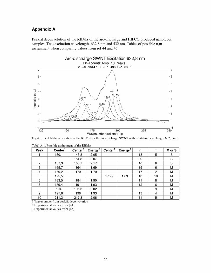
Two different SWNT samples, one arc-discharged and one HiPCO produced, were characterized using Raman spectroscopy. Each sample was investigated using two different laser excitations in order to probe different chiralities in the samples. For the 632,8 nm laser the effect was 1,0 mW and for 532 nm laser the effects was 0, 35 mW for the HiPCO and 0,78 mW for the arc-discharge produced sample. The spectra were acquired using a 20X objective, and the spot size was measured to be ~50 µm2. A 600 grooves/mm grating was first used to acquire a over view spectra, fig 20 and 22, and to be able to characterise the samples more precise a 1800 grooves/mm grating was used, fig 25. Typical integration time for the spectra was 1-2 s with 200-300 software integration giving a totally time of 10-20 min. We used a two step characterization process which involved first determining if the tubes in resonance were metallic or semiconducting, and then determining the chirality of each peak. To determine if the tubes are metallic or semiconducting we compare the wavenumber of each peak combined with the excitation energy used with an empirical Kataura plot. This tells us to which energy band the tubes belong. From the high resolution (1800gr/mm) spectra of the RBMs, a peak deconvolution was done using Peakfit software, and from this the chiralites of the tubes were assigned. In the chirality assignment we compare our measured RBM frequency with frequencies from literature.

Arc-discharged produced sample

The Raman spectra of the pristine arc-discharged sample are showed in fig 21, a) 632,8 nm and b) 532 nm excitation wavelength. In the spectra the RBM, D-band, G- and G+ are pointed out (see chapter 2.4.3 for theory about the Raman features). The inset spectrums in the top left corners shows the RBMs enlarged. From the wavenumbers of the RBMs we can estimate the diameter distribution in the sample by using equation 4 from section 2.3.3 with parameters for bundle sample [38]. For the sample we get diameters 1,22-1,65 nm which gives a average of ≈ 1,4 nm in agreement with ref 40.

35

By looking in the Kataura plot fig 22, we could assign the RBMs in fig 21 to metallic or semiconducting energy bands, see inset in fig 21. From the enlarged spectra of the RBM in the insets of fig 21 a and b, we see that different types of nanotubes are in resonance from the different laser excitations. In 21a there are almost only metallic tubes belonging to the M

E11 -

band in resonance and in 21b there are only semiconducting tubes from SE33

In the 632,8 nm excitation spectra the G- shows an asymmetric Breigt-Wigner-Fano peak shape which is typically for metallic nanotubes in bundles. This is in agreement with our assignment of the RBM to the metallic band. With the 532 nm excitation the G- peak shows a more symmetric Lorentian peak shape which is expected for samples containing mostly semiconducting tubes.

120 140 160 180 200 2200

10

20

30

40

50

200 400 600 800 1000 1200 1400 1600 1800

0

50

100

120 140 160 180 200 2200

5

10

15

20

Inte

nsity (

a.u

.)

Wavenumber (cm-1)

Metallictubes

Semi-conducting

tubes

G+

Inte

nsity (

a.u

.)

Wavenumber (cm-1)

Arc-discharge produced SWNT

Excitation 632,8 nm (1,96 eV) a)

RBMD

G-

G+

Inte

nsity (

a.u

.)

Wavenumber (cm-1)

Semi-

conductingtubes

200 400 600 800 1000 1200 1400 1600 1800

0

50

100

150

G-

Inte

nsity (

a.u

.)

Wavenumber (cm-1)


Excitation 532 nm (2,33 eV)

b)

RBM D

Fig 21 Raman spectra of pristine arc-discharge produced SWNT with different laser excitations, a) 632,8 nm b)

532 nm. Inset: the RBMs enlarged

Fig 24 Kataura plot showing the possible tubes in resonance from fig 21 marked by two shadowed areas. The circles represent experimentally measured values from ref 44 and the triangles are from ref 45. Filled circles and triangles represent metallic tubes and none filled represent semiconducting

100 120 140 160 180 200 220 240 260 280 300 320 340

1,4

1,6

1,8

2,0

2,2

2,4

2,6

2,8

3,0

E22

S

E11

M

Energ

y (

eV

)

Wavenumber (cm-1)

E33

S

36

HiPCO produced sample

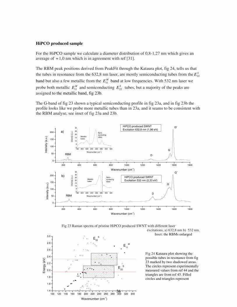
For the HiPCO sample we calculate a diameter distribution of 0,8-1,27 nm which gives an average of ≈ 1,0 nm which is in agreement with ref [31]. The RBM peak positions derived from PeakFit through the Kataura plot, fig 24, tells us that the tubes in resonance from the 632,8 nm laser, are mostly semiconducting tubes from the S

E22

band but also a few metallic from the ME11 band at low frequencies. With 532 nm laser we

probe both metallic ME11 and semiconducting S

E22 tubes, but a majority of the peaks are assigned to the metallic band, fig 23b. The G-band of fig 23 shown a typical semiconducting profile in fig 23a, and in fig 23b the profile looks like we probe more metallic tubes than in 23a, and it seams to be consistent with the RBM analyse, see inset of fig 23a and 23b.

180 200 220 240 260 280 300 3200

5

10

15

20

25

30

200 400 600 800 1000 1200 1400 1600 1800

0

50

100

150

200

180 200 220 240 260 280 300 3200

5

10

15

20

25

30

35

Inte

nsity (

a.u

.)

Wavenumber (cm-1)

Metallic

tubes

Semi-conducting

tubes

Inte

nsity (

a.u

.)

Wavenumber (cm-1)

HiPCO produced SWNT

Excitation 632,8 nm (1,96 eV) a)

RBM D

G-

G+

Inte

nsity (

a.u

.)

Wavenumber (cm-1)

Metallictubes

Semi-

conducing

tubes

200 400 600 800 1000 1200 1400 1600 1800

0

50

100

150

200

G+

G-

DRBM

Inte

nsity (

a.u

.)

Wavenumber (cm-1)

HiPCO produced SWNT


b)

Fig 23 Raman spectra of pristine HiPCO produced SWNT with different laser

excitations, a) 632,8 nm b) 532 nm. Inset: the RBMs enlarged

Fig 24 Kataura plot showing the possible tubes in resonance from fig 23 marked by two shadowed areas. The circles represent experimentally measured values from ref 44 and the triangles are from ref 45. Filled circles and triangles represent

100 120 140 160 180 200 220 240 260 280 300 320 340

1.4

1.6

1.8

2.0

2.2

2.4

2.6

2.8

3.0

E22

S

E11

M

En

erg

y (

eV

)

Wavenumber (cm-1)

E33

S

37

metallic tubes and none filled represent semiconducting. The analyse of the pristine samples based on their Raman spectra and the Kataura plot is summarized in table 2.

Table 2 Summary of analysis for the two different produced nanotubes Excitation

Sample 632.8 nm (1.96 eV) 532 nm (2.33 eV)

Arc-discharge ω < 160 Semiconducting Semiconducting

ω > 160 Metallic

HiPCO ω < 230 Metallic ω < 285 Metallic

ω > 230 Semiconducting ω > 285 Semiconducting

From the Peakfit deconvolution of the radial breathing modes we see that the peaks are composed of several smaller ones when fitted with Lorentzian peak shape see fig 25. A typical full with half maximum (FWHM) of around 7,5 cm-1 were chosen because the nanotubes were considered to be in bundles [38], and a residual r2 value better than 0,99 and a good visual agreement was achieved. The background and a linear baseline were subtracted before the deconvolution. The result from the deconvolution of the arc-discharge produced sample with 1,96 eV is represented in table 3, and data for the other samples with different laser excitation can be found in appendix A. The chirality assignment (n,m) is presented in table 3, and they are assigned from the measured RBMs compared with literature. According to Maultsch et al. ref 45 the RBM frequency alone will never be sufficient for assigning the chirality, because it depends on the environment of the tubes. Since none of the literature uses DMF to disperse their samples, a small error is being introduced. We estimate the error to be no more than ±0.1 eV.

197.55189.4

165.72

183.46

175.46

194

157.29

170.23

150.12

211.32

125 150 175 200 225 250

Wavenumber (cm^(-1))

-1

0

1

2

3

4

5

6

7

Inte

nsity (

a.u

.)

-1

0

1

2

3

4

5

6

7

38

Fig 25. Peakfit deconvolution of the RBM:s of arc-discharged sample. Excitation 632,8 nm

Table 3. Data from Peakfit deconvolution for the RBM compared with data from other groups to assign the

chirality index. M and S in last column stands for metallic and semiconducting respectively

Peak Center1 Center

2 Energy

2 Center

3 Energy

3 n m M or S

1 150,1 148,8 2,05 18 5 S

151,8 2,07 20 1 S

2 157,3 155,7 2,17 16 6 S

3 165,7 164 1,69 15 6 M

4 170,2 170 1,70 17 2 M

5 175,5 175,7 1,89 10 10 M

6 183,5 184 1,90 11 8 M

7 189,4 191 1,93 12 6 M

8 194 195,3 2,02 9 9 M

9 197,6 196 1,93 13 4 M

10 211,3 212,3 2,06 11 5 M 1 Wavenumber from peakfit deconvolution 2 Experimental values from [44] 3 Experimental values from [45]

Conclusion: The Raman spectra together with the Kataura plot made it possible to determine if the tubes in the samples were metallic or semiconducting and an index assignment could be done The intensity of the D-band of both samples is relative small compared to the intensity of the G-band so we can conclude that both pristine samples have a small amount of defects on the tube sidewalls.

4.2.2 Functionalized material To find out how the different nanotubes were affected by functionalization, Raman spectra from functionalized samples were compared with spectra from pristine samples. Two different laser excitation wavelengths were used to cover both metallic and semiconducting energy bands and to get a more complete picture of the samples. Two types of nanotubes were investigated, one arc-discharge produced and one HiPCO produced. There are special features in a Raman spectrum that one can look for to see if a sample is affected by the functionalization process. The intensity of the D-band should be higher compared to the G-band in a Raman spectrum acquired from a functionalized sample then for a spectrum from a pristine one, also the RBM modes are expected to be less intense [29]. The RBM analysis to se if the nanotubes in resonance are semiconducting or metallic are made using the Kataura plot, see section 4.2.1. The integrated intensities of the peaks are calculated using PeakFit software, see appendix B. Arc-discharge produced SWNT with laser excitation 632,8 nm (1,96 eV) and 532 nm

(2,33 eV)

39

Using the 632,8 nm excitation on the arc-discharge produced samples, almost only metallic tubes from the M

E11 energy are in resonance. The profile of the G- band is of BWF character, which also is a sign that the tubes probed are mostly metallic. Comparing the Raman spectrum acquired from the functionalized sample with the pristine, some differences in the intensities of the peaks can be observed (fig26). The RBMs are less intense and the D-band is more intense for the functionalized sample compared to the pristine. In the inset an enlarged picture of the RBM area can be seen, and the profile of the RBM show a small tendency of the higher wavenumbers to have lost more in intensity then the lower once. As integrated intensities are compared, the D/G ratio increases with a factor 2,08 and the RBM/G quota decreases to about half its value from the pristine sample. Table 4. Calculation of the integrated intensity for the different peaks relative the G-band (both G- and G+). Arc-

discharged produced, 632,8 nm excitation Integrated intensity

Sample RBM/G D/G

Pristine 0,096 0,156

Functionalized 0,049 0,326

Change, Funct./Pristine 0,52 2,08

100 120 140 160 180 200 220 2400

10

20

30

40

50

60

200 400 600 800 1000 1200 1400 1600 1800

0

25

50

75

100

Inte

nsity (

a.u

.)

Wavenumber (rel cm-1)

Metallic

tubes

Semiconducting

tubes

Inte

nsity (

a.u

.)



Excitation 632,8 nm (1,96 eV)

Pristine

Functionalized

Fig 26. Raman spectra of arc-discharge produced SWNT. Excitation 632,8 nm (1,96 eV). Red line is for pristine sample and blue is functionalized. The large spectrum is normalized after the G-band intensity. The inset show

the RBMs enlarged. The RBM peaks on the left hand side of the line belongs to tubes in resonance from

semiconducting energy band SE33 in the Kataura plot, and on the right hand side the tubes are metallic,

belonging to the ME11 band.

40

100 120 140 160 180 200 220 2400

5

10

15

20

25

200 400 600 800 1000 1200 1400 1600 1800

0

25

50

75

100

125

150

175

200

Inte

nsity (

a.u

.)


Semiconducting

tubes

Inte

nsity (

a.u

.)




Pristine

Functionalized

Fig 27. Raman spectra of arc-discharge produced SWNT. Excitation 532 nm (2,33 eV). The spectra are

normalized using the G-band intensity as reference. The inset show the RBMs enlarged. Only tubes from the

semiconducting energy band SE33 in the Kataura plot are in resonance.

When using the 532 nm excitation on the same arc-discharge samples, only semiconducting tubes from the S

E33 band are in resonance. As the acquired Raman spectra from pristine and functionalized samples are compared, fig27, only small changes can be seen. Looking at the enlarged picture of the RBM in the inset, the RBM modes show a drop in intensity but no direct change in profile. The D-band however shows very little change. The integrated intensities in table 5, show a decrease of a factor 0,53 in the RBM/G ratio after functionalization, and a smaller change of a factor 1,22 in the D/G ratio.

Table5 the Integrated intensities of the RBM and D-band compared to the integrated intensity of the G-band. Arc-discharge produced, 532 nm excitation.

Integrated intensity

Sample RBM/G D/G




HiPCO produced SWNT with laser excitation 632,8 nm (1,96 eV) and 532 nm (2,33 eV)

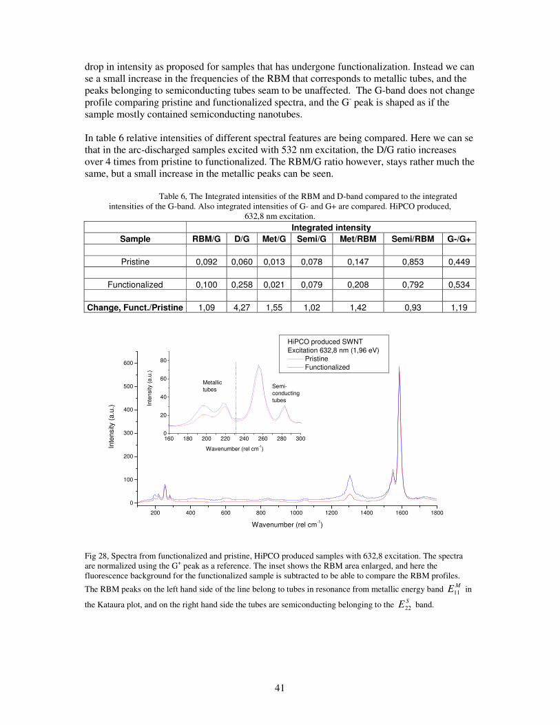
Using the 632,8 nm excitation on the HiPCO produced samples, both semiconducting tubes from the S

E22 energy band and metallic tubes from the ME11 energy band are in resonance.

Analysing the spectra from pristine and functionalized samples, fig 28, we se that the D-band is clearly more intense in the functionalized sample, as expected [29]. The RBM area does not

41

drop in intensity as proposed for samples that has undergone functionalization. Instead we can se a small increase in the frequencies of the RBM that corresponds to metallic tubes, and the peaks belonging to semiconducting tubes seam to be unaffected. The G-band does not change profile comparing pristine and functionalized spectra, and the G- peak is shaped as if the sample mostly contained semiconducting nanotubes. In table 6 relative intensities of different spectral features are being compared. Here we can se that in the arc-discharged samples excited with 532 nm excitation, the D/G ratio increases over 4 times from pristine to functionalized. The RBM/G ratio however, stays rather much the same, but a small increase in the metallic peaks can be seen.

Table 6, The Integrated intensities of the RBM and D-band compared to the integrated intensities of the G-band. Also integrated intensities of G- and G+ are compared. HiPCO produced,

632,8 nm excitation. Integrated intensity

Sample RBM/G D/G Met/G Semi/G Met/RBM Semi/RBM G-/G+

Pristine 0,092 0,060 0,013 0,078 0,147 0,853 0,449

Functionalized 0,100 0,258 0,021 0,079 0,208 0,792 0,534

Change, Funct./Pristine 1,09 4,27 1,55 1,02 1,42 0,93 1,19

160 180 200 220 240 260 280 3000

20

40

60

80

200 400 600 800 1000 1200 1400 1600 1800

0

100

200

300

400

500

600

Inte

nsity (

a.u

.)


Metallic

tubesSemi-

conducting

tubes

Inte

nsity (

a.u

.)


HiPCO produced SWNT

Excitation 632,8 nm (1,96 eV)

Pristine

Functionalized

Fig 28, Spectra from functionalized and pristine, HiPCO produced samples with 632,8 excitation. The spectra are normalized using the G+ peak as a reference. The inset shows the RBM area enlarged, and here the fluorescence background for the functionalized sample is subtracted to be able to compare the RBM profiles.

The RBM peaks on the left hand side of the line belong to tubes in resonance from metallic energy band ME11 in

the Kataura plot, and on the right hand side the tubes are semiconducting belonging to the SE22 band.

42

180 200 220 240 260 280 300 3200

5

10

15

20

25

30

600 1200 1800

0

80

160In

tensity (

a.u

.)


Metallic

tubes

Inte

nsity (

a.u

.)


HiPCO produced SWNT


Pristine

Functionalized

Fig. 29, Spectra from functionalized and pristine, HiPCO produced samples with 532 nm excitation. The spectra are normalized using the G+ peak as a reference. The inset shows the RBM area enlarged. All RBM peaks are

belonging to the ME11 band.

With 532 nm excitation the HiPCO produced samples show only metallic tubes in resonance from the M

E11 energy band. The spectra acquired, fig 29, show clearer differences when comparing pristine and functionalized samples. The D-band shows almost a two fold increase in intensity and splits up in to one large and one small peak. In the RBM area the main peak in the pristine spectra, about 275 cm-1, almost disappears, and the smaller peak at about 230 cm-1 increases slightly. The G- peaks show a small change, but both spectra show a BWF profile. As integrated intensities are compared, table ??, the RBM/G ratio decreases to almost half its value going from pristine to functionalized, and the D/G ratio goes up almost by a factor 3,6.

Table 7, integrated intensities of RBM and D-band compared to integrated intensity of the G-band. HiPCO sample, 532 nm excitation. Integrated intensity

Sample RBM/G D/G




Discussion: In the spectra from the arc-discharge produced sample acquired with 532 nm and 632,8 nm excitation wavelengths, we probe larger diameter semiconducting (~1,4 nm diameter) and metallic tubes. Looking at the RBM areas a similar drop in intensity can be seen in spectra acquired with both excitations. When mostly metallic tubes are probed the D-band is clearly more affected. This can be interpreted as if the metallic tubes are affected on a larger scale

43

than semiconducting tubes with larger diameters. In the HiPCO produced samples we probe metallic tubes and semiconducting tubes with smaller diameter (diameter < 1,1 nm). Here we see two scenarios. With 532 nm excitation light the RBM area show a significant metallic peak in the pristine sample which almost disappears when the sample is functionalized. Using 632,8 nm excitation light we probe the same diameter range as with 532 nm excitation, but here the tubes clearly belong to a semiconducting energy band. In this cases however, we see almost no change in the RBM area, which might be interpreted as if these tubes were not as affected from the functionalization as the metallic tubes of similar diameter. This is however only speculations, as the D-band in both cases sow almost the same increase in intensity. The metallic contribution to the RBM increases in both cases after functionalization. One explanation why metallic tubes seem to have been more could be the fact that metallic tubes seem to have more defects from the start Trying to explain this behaviour we turn to the Kataura plot to se what tubes, if any, the near surrounding to our energy and diameter intervals contain. We see three possible scenarios. One where the attached functional groups make nanotubes , hence a shift in RBM frequency. This however is not likely, as that would result in broadening of the peaks, which we don’t see in our spectra. The second and third option is positive or negative doping which would result in a decrease or increase in the resonance energies and hence it would be possible for tubes to fall out of or in to resonance. Looking at the Kataura plot and our acquired spectra, it seems most probable if the functional groups have altered the electronic structure and made the energy gap on the metallic tubes larger, making the bands in the Kataura plot move upwards for affected tubes.

Table 8, integrated intensities compared.

istine

Funk

IG

IDIG

ID

Pr

.

Arc-discharge CNTs HiPCO CNTs

Laser Red Green Red Green

D-band change 2,08 1,22 4,27 3,6

Tube type Metallic Semicond. Both M and S Metallic

Conclusions: Both metallic and semiconducting tubes are affected from the functionalization, but metallic tubes and tubes with smaller diameters seam to be affected in higher grade compared to semiconducting tubes with larger diameters.

44

4.2.3 Composite material based on MWCNT (SiComp samples) Three different MWCNT- polymer composites, CNT1, CNT2, CNTREF from SiComp were investigated. In order to analyse the composites the raw MWCNT used in the composites and an epoxy polymer sample, LY564 was investigated. The samples were investigated with Raman spectroscopy. First the spectra of pristine MWCNT and of the polymers without nanotubes where acquired. In the MWCNT spectrum a distinct D-peak and a G-band can be seen, see fig 31a. In the spectra of the polymer LY564 several peak where found, fig 31b. (No further assignment of these peaks was done).

250 500 750 1000 1250 1500 1750 2000

0

20

40

60

80

250 500 750 1000 1250 1500 1750 2000

0

20

40

60

80

Inte

nsity (

a.u

.)


LY564b)

Inte

nsity (

a.u

.)


MWCNTa)

Fig 31, Spectrum of a) MWCNT b) Polymer LY564. The dotted line at 1320 cm-1 is just a guide line for the eye.

250 500 750 1000 1250 1500 1750 2000

0

20

40

60

80 250 500 750 1000 1250 1500 1750 2000

0

20

40

60

80

Inte

nsity (

a.u

.)


Small D-peak in CNT1b)

Inte

nsity (

a.u

.)


Strong D-peak in CNT1

a)

Fig 32. Two different profile of CNT1 a) Strong D-peak b) Small D-peak.

The dotted line at 1320 cm-1 is just a guide line for the eye.

45

In the composite polymers named CNT1, CNT2 and CNTREF different Raman profile was found. The profiles acquired were one profile with a big D-peak, one with a small D-peak and one profile with no D-peak in the polymer spectrum. In some spots no Raman signal at all was found or a very low signal which made it impossible to determent the category the sample belonged to. The spectrum of the two profiles containing the D-band of the MWCNTs are shown in Fig 32 It is only in the wavenumber interval 1250-1600 cm-1 that any difference from the spectrum of the polymer can bee detected. The peak at 1550-1600 cm-1 becomes broader with the contribution of the G-band from the MWCNTs. By acquiring spectra in different points in the sample, the homogeneity of the sample in terms of MWCNT distribution in the polymer matrix was investigated. In table 9 the results of counting the different profiles in the samples are shown. In the strange signal points the intensity of the spectra was increasing when integrating and the measurement had to be stopped. Table 9, the number of different profiles in the spectra of the composites, and the percentage of each type. In the

columns the type of spectra then the number and percentage of each profile is presented. CNT1 CNT2 CNTREF

Type Nr of spectra % Nr of spectra % Nr of spectra %

Strong D 2 10 7 27 7 23

Small D 3 15 5 19 1 3

No D 11 55 2 8 14 45

No Signal 4 20 9 35 8 26

Strange Signal 3 12 1 3

Total 20 100 26 100 31 100

From the data in table 9, we can suspect that the MWCNTs are better dispersed in the CNT2 sample compared to the CNT1 and CNTREF samples. Still we think that the nanotubes are not that well dispersed due to the many spectra lacking signs of a D- and G-band. Comparing the spectra of the raw polymers and the composite samples, we see no direct change in the spectra except for the appearance of the D- and G-band. We interpret this as a sign of weak interaction between the polymer and the MWCNTs. Examples of changes that would show stronger interaction may be shift of peaks, broadening of peaks, splitting of peaks or new peaks.

46

4.3 Raman study of polymerized fullerenes In order to characterize two different types of polymerized fullerenes, Raman spectroscopy was used. Because of high fluorescence background when exciting with laser of 1,96 eV only laser with 2,33 eV was used.

4.3.1 1D C60 polymers Spectra from several samples of C60 that had been polymerized at high temperature-pressure were examined. Within each sample two different profiles were found fig 33. The frequency of the pentagonal-pinch mode Ag(2) for the two different profiles was 1457 cm-1 (fig33b) and 1463 cm-1 (fig33a). According to section 2.3.3 the Ag(2) for the one dimensional orthorhombic polymer of C60 should be 1459 cm-1. So the profile we found with a pp mode of 1457 cm-1 can be related to the 1D orthorhombic fullerene. The other profile probably belongs to dimers of C60 that has not completely polymerized to the orthorhombic phase. The pentagonal-pinch mode was found to be 1464 cm-1 for a dimerized state.

200 400 600 800 1000 1200 1400 1600 1800

0

5

10

15

20

200 400 600 800 1000 1200 1400 1600 1800

0

5

10

15

20

Inte

nsity (

a.u

.)


a)

Inte

nsity (

a.u

.)


b)

1420 1440 1460 1480

4

8

12

16

20

Inte

nsity

(a

.u.)


1420 1440 1460 1480

4

8

12

16

20

Inte

nsi

ty (

a.u

.)


Fig 33. Raman spectra of polymerized fullerenes. Same sample two different spots.

Inset: the pentagonal-pinch mode enlarged From the spectra we can deduce some other peaks too. We have the breathing mode Ag(1) at 488 cm-1 and some Hg modes, Hg(2) 451 cm-1, Hg(8) 1572 cm-1 and Hg(8) 1559 cm-1. We have peaks at 257 cm-1, 708 cm-1 and 1303 cm-1 which don’t match any of the modes of the pristine C60. There are also modes that are not Raman active in pristine C60 that now has become active because the change in symmetry, for example the peaks F1g(2) at 965 cm-1 and Gg(3) 1191 cm-1. There is one peak at 707,5 cm-1 which doesn’t match any of the peaks in the reference. The peaks are summarized in table 10.

47

Table 10. Vibrational modes of monomeric C60, our measured values for polymeric C60 and values from references of the 1-D orthorhombic structure.

Monomeric C60 [46] Measured

values 1-D orthorhomic

C60 [35] 1-D orthorhomic

C60 [33]

257,4 256

431 Hg(2) 450,7 450

495 Ag(1) 488,1 488

707,5

973 F1g(2) 961,9 965

1199 Gg(3) 1191 1192

1302,5 1297

1330 Gg(4) 1315,2 1310

1425 Hg(7) 1429 1432

1470 Ag(2) 1456,8 1457 1459

1567 Hg(8) 1558,6 1560

1576 Hg(8) 1572,5 1572

4.3.2 2D C60 polymers For the 2D polymer, fig 34, the pentagonal-pinch mode is at 1448 cm-1 and according to section 2.3.3 it should be 1447 cm-1 or 1449 cm-1. The peaks are summarized in table 11 where the bold numbers are the larges peaks. We see that the most intense peaks except for the pp mode are modes that are not Raman active in pristine C60. Peaks that become active in the polymerized fullerene are F2g(1) at 536,3 cm-1, F1g(1) at 588,4 cm-1, Gg(2) at 954,4 cm-1, F2u(4) at 1048,3 cm-1, F1g(3) at 1463,1 cm-1 and F2g(4) at 1542,5 cm-1. For the polymerized C60 samples there is a shift of the breathing mode Ag(1) mode towards lower frequencies compared to the monomeric C60. This could be explained by the covalent bonding between the C60 created in the polymerization that make the entire matrix more rigid. The intensity of the Ag(1) mode in monomeric C60 is usually the second most intensive peak in the Raman spectrum, but in the polymers it is much less distinct. There is two peaks in the spectra with wavenumbers 1206,0 cm-1 and 1406,3 cm-1 which doesn’t match any of the peaks from the reference and could not be explain.

48

250 500 750 1000 1250 1500 1750 2000

0

5

10

15

20

25

30

1400 1420 1440 1460 1480 15000

10

20

30

Inte

nsity (

a.u

.)


Green Laser (2,33 eV)

2D.1Pentagonal-pinch mode

Fig 34 Raman spectra of 2D polymerized fullerenes

Table 11 Vibrational modes of monomeric C60, our measured values for polymeric C60 and values from

references of the 2-D tetragonal structure.

Monomeric C60 [46] Measured

values 2-D tetragonal C60

[35] 2-D tetragonal C60

[33]

272 Hg(1) 281,2 282

431,4 432

495 Ag(1) 486,9 487

541 F2g(1) 536,3 538

568 F1g(1) 588,4 588

664,2 667

684,9 685

778 Hg(4) 749,4 748

961 Gg(2) 954,4 955

1038,4 1034

1038 F2u(4) 1048,3 1044

1102 Hg(g) 1106,5 1109

1206

1301,1 1296

1406,3

1470 Ag(2) 1448,4 1449 1447

1484 F1g(3) 1463,1 1465

1544 F2g(4) 1542,5 1544

1576 Hg(8) 1571,4 1573

Conclusions: Raman spectroscopy showed to be a very powerful tool for characterization of different polymeric phases of fullerenes due to the different features in spectrum. Especially the pentagonal-pinch mode peak is useful because of its shift for the different polymers.

49

5 Summary

5.1 Summary We build a pressure control box to regulate and fine tune pressure in the membrane in our membrane diamond anvil cell (MDAC). Using ruby fluorescence method, we calibrate the pressure in the membrane against the generated pressure in the cell. This resulted in both a pre-indentation pressure curve for hardened stainless steel gaskets and a pressure curve for pressure in the membrane against generated pressure in the DAC. Raman spectroscopy was used to characterize carbon nanostructures. Spectra were acquired from fullerene and nanotube samples with 532 nm (2,33 eV) and 632,8 nm (1,96 eV) excitation lights. Different types of polymeric fullerene samples were characterized in order to determine their structure. The nanotubes examined were synthesized by HiPCO and Arc-discharged methods, and the purpose was to se how a certain type of functionalization affects the nanotubes. Spectra were acquired of pristine and functionalized samples with 532 nm (2,33 eV) and 632,8 nm (1,96 eV) excitations and compared. Both metallic and semiconducting tubes are investigated to se if any special kind of nanotubes is more affected of the functionalization than others. Multi wall CNT (MWNT) - epoxy composites, manufactured by SiComp, were examined with Raman spectroscopy to se how the MWNT interacted with the epoxy matrix and to get an estimation of how well dispersed the MWNTs were in the matrix. Spectra were acquired from epoxy and MWNTs one by one, and then compared with spectra acquired from the composites.

5.2 Conclusions Conclusions high pressure:

• Several regions on PDAC vs PGAS calibration curve: Hydrostatic (below 10 GPa).

1) Below pre-indent pressure 2) Above pre-indent pressure

Non-hydrostatic pressure (above 10 GPa)

• We calibrated (linear dependence Pdac vs Pgas) the gas loading DAS system

• We established recommendations for further experiments different “sensitivity” in exponent vs linear regions

• Centring of the gasket hole is very important. (Off centre 10 µm is already

unacceptable)

50

Conclusions characterisation, nanotubes: The Raman spectra together with the Kataura plot make it possible to determine if the tubes in a sample are metallic or semiconducting. Conclusions functionalized nanotubes: Both metallic and semiconducting tubes are affected from the functionalization, but metallic tubes and tubes with smaller diameters seam to be affected in higher grade compared to semiconducting tubes with larger diameters. Conclusions characterisation, fullerenes: Raman spectroscopy showed to be a very powerful tool for characterization of different polymeric phases of fullerenes due to the different features in spectrum. Especially the pentagonal-pinch mode peak is useful because of its shift for the different polymers.

5.3 Recommendations for future work Measurements on isolated SWNTs are needed to be done, both Raman and PL. To investigate the samples using more different excitation sources.

Extra

Results from the investigation on functionalized carbon nanotubes has been presented at European Materials Research Society (EMRS) Conference in Strasbourg, France 2007 and are to be published in Physica E. The results are also to be presented at International Conference on Nano Science and Technology (ICN+T2007), July 2007 in Stockholm, Sweden.

51

Ref [1] (Science and Technology Encyclopedia information about High-pressure physics McGraw-Hill Encyclopedia of Science and Technology. Copyright © 2005 by The McGraw-Hill Companies, Inc. All rights reserved. More from Science and Technology Encyclopedia) http://www.answers.com/topic/high-pressure-physics [2] Wang, X.B. ; Shen, Z.X.; Tang, S.H.; Kuok, M.H., Near infrared excited micro-Raman

spectra of 4:1 methanol-ethanol mixture and ruby fluorescence at high pressure, Journal of Applied Physics, v 85, n 12, 15 June 1999, p 8011-17 [3] Dunstan, D.J., Theory of the gasket in diamond anvil high-pressure cells, Review of Scientific Instruments, v 60, n 12, Dec. 1989, p 3789-95 [4] R. Saito, G. Dresselhaus, M.S. Dresselhaus, Physical Properties of Carbon Nanotubes, Imperial College Press, London, 1998. [5] Kroto, H.W.; Heath, J.R.; O'Brien, S.C.; Curl, R.F.; Smalley, R.E., C60:

Buckminsterfullerene, Nature, v 318, n 6042, 14 Nov. 1985, p 162-3 [6] M.S. Dresselhaus, G. Dresselhaus, P. Eklund, Science of Fullerenes and Carbon

Nanotubes, January 1996, c. 965pp., ISBN 0-12-221820-5

[7] Dresselhaus, S.; Dresselhaus, G.; Eklund, P.C., Raman scattering in fullerenes, Journal of Raman Spectroscopy, v 27, n 3-4, March-April 1996, p 351-71 [8] Nunez-Regueiro, M.; Marques, L.; Hodeau, J.-L.; Bethoux, O.; Perroux, M., Polymerized

fullerite structures, Physical Review Letters, v 74, n 2, 9 Jan. 1995, p 278-81 [9] Blank, V.D.; Buga, S.G.; Serebryanaya, N.R.; Dubitsky, G.A.; Mavrin, B.N.; Popov, M.Yu.; Bagramov, R.H.; Prokhorov, V.M.; Sulyanov, S.N.; Kulnitskiy, B.A.; Tatyanin, Ye.V., Structures and physical properties of superhard and ultrahard 3D polymerized

fullerites created from solid C60 by high pressure high temperature treatment, Carbon, v 36, n 5-6, 1998, p 665-70 [10] Õsawa Eiji, Dordrecht ; Kluwer Academic Publishers, Perspectives of Fullerene

Nanotechnology, cop. 2002, http://proxy.lib.luth.se/login?url=http://ebooks.springerlink.com/AccessProduct.aspx?ProductId=78527 ; Endast för användare inom LTU

[11] Iijima, S., Helical microtubules of graphitic carbon, Nature, v 354, n 6348, 7 Nov. 1991, p 56-8 [12] Iijima, S.; Ichihashi, T., Single-shell carbon nanotubes of 1-nm diameter, Nature, v 363, n 6430, 17 June 1993, p 603-15 [13] Dresselhaus, M.S.; Dresselhaus, G.; Saito, R.; Jorio, A., Raman spectroscopy of carbon

nanotubes, Physics Reports, v 409, n 2, March 2005, p 47-99

52

[14] Samsonidze, Ge.G.; Saito, R.; Kobayashi, N.; Gruneis, A.; Jiang, J.; Jorio, A.; Chou, S.G.; Dresselhaus, G.; Dresselhaus, M.S., Family behavior of the optical transition energies

in single-wall carbon nanotubes of smaller diameters, Applied Physics Letters, v 85, n 23, Dec 6, 2004, p 5703-5705 [15] Kay Hyeok An.; Young Hee Lee., Electronic-structure engineering of carbon nanotubes, Nano, v 1, n 2, 2006, p 115–138 [16] Hjortstam, O.; Isberg, P.; Soderholm, S.; Dai, H., Can we achieve ultra-low resistivity in

carbon nanotube-based metal composites?, Applied Physics A (Materials Science Processing), v A78, n 8, May 2004, p 1175-9 [17] Dresselhaus, M.S.; Dresselhaus, G.; Charlier, J.C.; Hernandez, E., Electronic, thermal

and mechanical properties of carbon nanotubes, Philosophical Transactions of the Royal Society London, Series A (Mathematical, Physical and Engineering Sciences), v 362, n 1823, 15 Oct. 2004, p 2065-98 [18] Pop, Eric; Mann, David; Wang, Qian; Goodson, Kenneth; Dai, Hongjie, Thermal

conductance of an individual single-wall carbon nanotube above room temperature, Nano Letters, v 6, n 1, January, 2006, p 96-100 [19] Yanhong Hu; Shenderova, O.A.; Zushou Hu; Padgett, C.W.; Brenner, D.W., Carbon

nanostructures for advanced composites, Reports on Progress in Physics, v 69, n 6, June 2006, p 1847-95 [20] Cadek, M.; Coleman, J.N.; Barron, V.; Hedicke, K.; Blau, W.J., Morphological and

mechanical properties of carbon-nanotube-reinforced semicrystalline and amorphous

polymer composites, Applied Physics Letters, v 81, n 27, Dec 30 2003, 2002, p 5123-5125 [21] Ruan, S.L., Hong Kong Univ. of Sci./Technology); Gao, P.; Yang, X.G.; Yu, T.X., Toughening high performance ultrahigh molecular weight polyethylene using multiwalled

carbon nanotubes, Polymer, v 44, n 19, Aug 21, 2003, p 5643-5654 [22] Liu, Tianxi; Phang, In Yee; Shen, Lu; Chow, Shue Yin; Zhang, Wei-De, Morphology

and mechanical properties of multiwalled carbon nanotubes reinforced nylon-6 composites, Macromolecules, v 37, n 19, Sep 21, 2004, p 7214-7222 [23] Chang, T.E.; Jensen, L.R.; Kisliuk, A.; Pipes, R.B.; Pyrz, R.; Sokolov, A.P., Microscopic

mechanism of reinforcement in single-wall carbon nanotube/polypropylene nanocomposite, Polymer, v 46, n 2, Jan 12, 2005, p 439-444 [24] Belin, T.; Epron, F., Characterization methods of carbon nanotubes: A review, Materials Science and Engineering B: Solid-State Materials for Advanced Technology, v 116, n 2, Jan 25, 2005, p 105-118 [25] Parker, Deborah Holmes; Chatterjee, Kuntal; Wurz, Peter; Lykke, Keith R.; Pellin, Michael J.; Stock, Leon M.; Hemminger, John C., Fullerenes and giant fullerenes: Synthesis,

separation, and mass spectrometric characterization, Carbon, v 30, n 8, 1992, p 1167-1182

53

[26] Terranova, Maria Letizia; Sessa, Vito; Rossi, Marco, The world of carbon nanotubes: An

overview of CVD growth methodologies, Chemical Vapor Deposition, v 12, n 6, June, 2006, p 315-325 [27] Rao, A.M.; Zhou, Ping; Wang, Kai-An; Hager, G.T.; Holden, J.M.; Wang, Ying; Lee, W.-T.; Bi, Xiang-Xin; Eklund, P.C.; Cornet, D.S.; Duncan, M.A.; Amster, I.J., Photoinduced

polymerization of solid C60 films, Science, v 259, n 5097, Feb 12, 1993, p 955-957 [28] Sundqvist, B., Fullerenes under high pressures, Advances in Physics, v 48, n 1, February, 1999, p 1-134 [29] Bahr, J.L.; Tour, J.M., Covalent chemistry of single-wall carbon nanotubes, Journal of Materials Chemistry, 12, May 2002, p 1952-1958 [30] Dyke, Christopher A.; Tour, James M., Covalent functionalization of single-walled

carbon nanotubes for materials applications, Journal of Physical Chemistry A, v 108, n 51, Dec 23, 2004, p 11151-11159 [31] Liu, Jie; Zubiri, Mireia Rodriguez I.; Dossot, Manuel; Vigolo, Brigitte; Hauge, Robert H.; Fort, Yves; Ehrhardt, Jean-Jacques; McRae, Edward, Sidewall functionalization of single-

wall carbon nanotubes (SWNTs) through aryl free radical addition, Chemical Physics Letters, v 430, n 1-3, Oct 19, 2006, p 93-96 [32] Strano, Michael S.; Dyke, Christopher A.; Usrey, Monica L.; Barone, Paul W.; Allen, Mathew J.; Shan, Hongwei; Kittrell, Carter; Hauge, Robert H.; Tour, James M.; Smalley, Richard E., Electronic structure control of single-waited carbon nanotube Functionalization, Science, v 301, n 5639, Sep 12, 2003, p 1519-1522 [33] Wagberg, T.; Soldatov, A.; Sundqvist, B., Spectroscopic study of phase transformations

between orthorhombic and tetragonal C60 polymers, European Physical Journal B, v 49, n 1, Jan. 2006, p 59-65 [34] Meletov, K.P.; Arvanitidis, J.; Kourouklis, G.A.; Prassides, K.; Iwasa, Y., Structural

stability of the rhombohedral 2D polymeric phase of C60 studied by in-situ Raman scattering

at pressures up to 30 GPa, Chemical Physics Letters, v 357, n 3-4, 10 May 2002, p 307-13 [35] Davydov, V.A.; Kashevarova, L.S.; Rakhmanina, A.V.; Senyavin, V.M.; Ceolin, R.; Szwarc, H.; Allouchi, H.; Agafonov, V., Spectroscopic study of pressure-polymerized phases

of C60, Physical Review B (Condensed Matter), v 61, n 18, 1 May 2000, p 11936-45 [36] Persson, P.-A.; Edlund, U.; Jacobsson, P.; Johnels, D., NMR and Raman characterization

of pressure polymerized C60, Chemical Physics Letters, v 258, n 5-6, 1996, p 540

[37] Persson, P.A.; Andersson, O.; Jacobsson, P.; Soldatov, A.; Sundqvist, B.; Wagberg, T., Physical properties of high-pressure polymerized C60, Journal of Physics and Chemistry of Solids, v 58, n 11, Nov, 1997, p 1881-1885 [38] Paillet, M.; Poncharal, Ph.; Zahab, A.; Sauvajol, J.-L.; Meyer, J.C.; Roth, S., Vanishing

of the Breit-Wigner-Fano component in individual single-wall carbon nanotubes, Physical Review Letters, v 94, n 23, Jun 17, 2005, p 1-4

54

[39] Jorio, A.; Saito, R.; Hafner, J.H.; Lieber, C.M.; Hunter, M.; McClure, T.; Dresselhaus, G.; Dresselhaus, M.S., Structural (n, m) determination of isolated single-wall carbon

nanotubes by resonant Raman scattering, Physical Review Letters, v 86, n 6, Feb, 2001, p 1118-1121 [40] Liu, Jie; Zubiri, Mireia Rodriguez i; Vigolo, Brigitte; Dossot, Manuel; Fort, Yves; Ehrhardt, Jean-Jacques; McRae, Edward, Efficient microwave-assisted radical

functionalization of single-wall carbon nanotubes, Carbon, v 45, n 4, April, 2007, p 885-891 [41] Meletov, K.P.; Arvanitidis, J.; Tsilika, E.; Assimopoulos, S.; Kourouklis, G.A.; Ves, S.; Soldatov, A.; Prassides, K., Pressure-induced phase in tetragonal two-dimensional polymeric

C60, Physical Review B (Condensed Matter), v 63, n 5, 1 Feb. 2001, p 054106/1-4 [42] Shen, Yongrong; Kumar, Ravhi S.; Pravica, Michael; Nicol, Malcolm F., Characteristics

of silicone fluid as a pressure transmitting medium in diamond anvil cells, Review of Scientific Instruments, v 75, n 11, November 2004, p 4450-4454 [43] Spain, I L; Dunstan D J., The technology of diamond anvil high-pressure cells: II.

Operation and use, J. Phys. E: Sci. 1989, p 923-933 [44] http://www.fisica.ufmg.br/~adojorio/Download.htm [45] J. Maultzsch; H. Telg; S. Reich; and C. Thomsen., Radial breathing mode of single-

walled carbon nanotubes: Optical transition energies and chiral-index assignment, PHYSICAL REVIEW B 72, 205438 _2005_ [46] Martin., Observation and assignment of silent and higher-order vibrations in the infrared

transmission of C60 crystals, Physical review. B, Condensed matter [0163-1829], 1994 vol:50 nr:1 sid:173 -83

55

Appendix A

Peakfit deconvolution of the RBM:s of the arc-discharge and HIPCO produced nanotubes samples. Two excitation wavelength, 632,8 nm and 532 nm. Tables of possible n,m assignment when comparing values from ref 44 and 45.

Arc-discharge SWNT Excitation 632,8 nmPk=Lorentz Amp 10 Peaks

r^2=0.996447 SE=0.13436 F=1363.51

197.55189.4

165.72

183.46

175.46

194

157.29

170.23

150.12211.32

125 150 175 200 225 250

Wavenumber (rel cm^(-1))

-1

0

1

2

3

4

5

6

7

Inte

nsity (

a.u

.)

-1

0

1

2

3

4

5

6

7

Fig A:1. Peakfit deconvolution of the RBM:s for the arc-discharge SWNT with excitation wavelength 632,8 nm Tabel A:1. Possible assignment of the RBM:s

Peak Center1 Center

2 Energy

2 Center

3 Energy

3 n m M or S

1 150,1 148,8 2,05 18 5 S

151,8 2,07 20 1 S

2 157,3 155,7 2,17 16 6 S

3 165,7 164 1,69 15 6 M

4 170,2 170 1,70 17 2 M

5 175,5 175,7 1,89 10 10 M

6 183,5 184 1,90 11 8 M

7 189,4 191 1,93 12 6 M

8 194 195,3 2,02 9 9 M

9 197,6 196 1,93 13 4 M

10 211,3 212,3 2,06 11 5 M 1 Wavenumber from peakfit deconvolution 2 Experimental values from [44] 3 Experimental values from [45]

56

Arc-discharge SWNT Excitation 532 nmPk=Lorentz Amp 10 Peaks

r^2=0.997786 SE=0.172834 F=1892.82

171.42

185.5

166.35

158.47148.62 191.21

176.63

125 150 175 200 225 250


-5

0

5

10

15In

ten

sity (

a.u

.)

-5

0

5

10

15

Fig A:2. Peakfit deconvolution of the RBM:s for the arc-discharge SWNT with excitation wavelength 532 nm Tabel A:2. Possible assignment of the RBM:s

Peak Center1 Center

2 Energy

2 n m M or S

1 148,6 148,8 2,05 18 5 S

2 158,5 155,7 2,17 16 6 S

161 2,27 13 9 S

3 166,4 165,5 2,60 18 1 S

4 171,4 172,5 2,30 16 3 S

5 176,6 174,8 2,29 17 1 S

6 185,5 185,5 2,44 14 4 S

7 191,2 190,1 2,43 16 0 S 1 Wavenumber from peakfit deconvolution 2 Experimental values from [44]

HiPCO SWNT Excitation 632,8 nmPk=Lorentz Amp 10 Peaks

r^2=0.996258 SE=0.404873 F=1525.96

258.12

283.92220.51

198.35 218.33

192.88

254.17

264.64 283.41

222.58

252.12

205.45

247.18

213.99

150 200 250 300 350


-5

0

5

10

15

20

25

30

35

Inte

nsity (

a.u

.)

-5

0

5

10

15

20

25

30

35

Fig A:3. Peakfit deconvolution of the RBM:s for the HiPCO SWNT with excitation wavelength 632,8 nm

57

Tabel A:3. Possible assignment of the RBM:s

Peak Center1 Center

2 Energy

2 Center

3 Energy

3 n m M or S

1 192,9 191 1,93 12 6 M

2 198,4 199,5 1,93 14 2 M

3 205,5 204,7 2,05 10 7 M

4 214,0 212,3 2,06 11 5 M

5 218,3 218 2,05 12 3 M

6 220,5 221,8 1,76 11 4 S

7 222,6 222,9 2,02 13 1 M

8 247,2 246 1,74 8 6 S

9 252,1 252,1 1,95 10 3 S

10 254,2 256 2,03 11 1 S

11 258,1 257,5 1,74 9 4 S

12 264,6 265 1,69 10 2 S

13 283,4 283,1 1,93 7 5 S

14 283,9 1 Wavenumber from peakfit deconvolution 2 Experimental values from [44] 3 Experimental values from [45]

HiPCO SWNT Excitation 532 nmPk=Lorentz Amp 10 Peaks

r^2=0.987252 SE=0.372817 F=555.584

271.6

262.49

292.12

247.58

239.03

229.02

216.54274.97

150 200 250 300 350


-5

0

5

10

15

Inte

nsity (

a.u

.)

-5

0

5

10

15

Fig A:4. Peakfit deconvolution of the RBM:s for the HiPCO SWNT with excitation wavelength 532 nm Tabel A:4. Possible assignment of the RBM:s

Peak Center1 Center

2 Energy

2 Center

3 Energy

3 n m M or S

1 216,5 218 2,05 12 3 M

2 229,0 228 2,24 9 6 M

3 239,0 239 2,22 10 4 M

4 247,6 247,8 2,45 7 7 M

5 262,5 262,7 2,47 8 5 M

6 271,6 272,7 2,43 9 3 M

7 275,0 276,3 2,38 10 1 M

8 292,1 291,4 2,38 10 0 S 1 Wavenumber from peakfit deconvolution 2 Experimental values from [44] 3 Experimental values from [45]

58

Appendix B

Peakfit deconvolution of the peaks in spectra shown in figures and data from Peakfit presented in tables

CLIPBRD.PRNPk=Lorentz Amp 5 Peaks

r^2=0.989232 SE=2.88599 F=2585.49

1586.6

1329.4

1560.8

167.95

176.55

0 500 1000 1500 2000-50

0

50

100

150

200

250

300

-50

0

50

100

150

200

250

300

Fig B:1. Peakfit deconvolution of the spectra for the pristine arc-discharge SWNT with excitation wavelength 532 nm Tabel B:1. Data from Peakfit the pristine arc-discharge SWNT with excitation wavelength 532 nm Peak Type

Amplitude Center FWHM Int Area % Area

1 Lorentz Amp 22,50578 167,9533 17,62985 595,929 4,889033

2 Lorentz Amp 12,12001 176,5488 26,88391 481,5107 3,950339

3 Lorentz Amp 18,80734 1329,365 67,19398 1922,592 15,77305

4 Lorentz Amp 77,37003 1560,847 19,75309 2363,699 19,39191

5 Lorentz Amp 278,5933 1586,596 15,81149 6825,366 55,99566

Total 12189,1 100

59

CLIPBRD.PRNPk=Lorentz Amp 5 Peaks

r^2=0.986509 SE=2.04788 F=2057.98

1586.9

182.07

168.42 1332.7

1561.5

0 500 1000 1500 2000-50

0

50

100

150

200

-50

0

50

100

150

200

Fig B:2. Peakfit deconvolution of the spectra for the functionalized arc-discharge SWNT with excitation wavelength 532 nm Tabel B:2. Data from Peakfit the functionalized arc-discharge SWNT with excitation wavelength 532 nm Peak Type

Amplitude Center FWHM Asym50

FW Base Asym10

1 Lorentz Amp 7,555156 168,4199 17,60522 1 58,68406 1

2 Lorentz Amp 5,273333 182,0726 29,61866 1 98,72886 1

3 Lorentz Amp 16,50331 1332,716 55,90829 1 186,361 1

4 Lorentz Amp 51,22684 1561,458 22,45682 1 74,85605 1

5 Lorentz Amp 184,6488 1586,893 13,47388 1 44,91292 1

Peak Type

Anlytc Area % Area Int Area % Area Centroid

Moment2

1 Lorentz Amp 208,9319 2,742366 199,8463 2,671908 177,7569 4805,063

2 Lorentz Amp 245,3412 3,220262 230,3923 3,080302 197,0553 8072,493

3 Lorentz Amp 1449,329 19,02339 1411,186 18,8673 1323,844 14643,78

4 Lorentz Amp 1807,031 23,71845 1775,352 23,73613 1554,845 6001,998

5 Lorentz Amp 3908,039 51,29554 3862,759 51,64436 1582,664 3617,482

Total 7618,672 100 7479,536 100

60

CLIPBRD.PRNPk=Mixed 5 Peaks

r^2=0.993413 SE=2.45594 F=3951.49

272.041325.5

1584

244.9

1529.5

0 500 1000 1500 2000-50

0

50

100

150

200

250

-50

0

50

100

150

200

250

Fig B:3. Peakfit deconvolution of the spectra for the pristine HiPCO SWNT with excitation wavelength 532 nm Tabel B:3. Data from Peakfit the pristine HiPCO SWNT with excitation wavelength 532 nm Peak Type


FW Base Asym10

1 Lorentz Amp 5,849757 244,8989 12,34281 1 41,14269 1

2 Lorentz Amp 24,00826 272,0446 13,66181 1 45,53935 1

3 Lorentz Amp 30,65333 1325,475 45,41713 1 151,3904 1

4 BWF[UDF1] 96,20542 1529,493 75,01306 0,795376 279,8714 0,490404

5 Lorentz Amp 181,2622 1583,969 25,89313 0,999999 86,31044 1

Peak Type


Moment2

1 Lorentz Amp 113,4153 111,7168 0,473447 249,6516 3322,7

2 Lorentz Amp 515,2152 507,9076 2,152474 276,8794 3671,887

3 Lorentz Amp 2186,841 2140,516 9,071347 1318,459 11963,66

4 BWF[UDF1] Unknown 13625,97 57,74585 1336,395 122210

5 Lorentz Amp 7372,45 7210,342 30,55689 1575,828 6914,737

Total 23596,45 100

61


r^2=0.995293 SE=2.09372 F=3896.73

269.73

1324.6

1584.7

244.78

1536.7

230.24

1380.7

0 500 1000 1500 2000-50

0

50

100

150

200

-50

0

50

100

150

200

Fig B:4. Peakfit deconvolution of the spectra for the functionalized HiPCO SWNT with excitation wavelength 532 nm Tabel B:4. Data from Peakfit the functionalized HiPCO SWNT with excitation wavelength 532 nm Peak Type


FW Base Asym10

1 Lorentz Amp 6,226779 230,2381 14,84051 1 49,46836 1

2 Lorentz Amp 3,414552 244,781 13,34902 1 44,49674 1

3 Lorentz Amp 4,908359 269,735 13,58739 1 45,29129 1

4 Lorentz Amp 73,02905 1324,648 61,30959 1 204,3653 1

5 Lorentz Amp 14,71174 1380,662 14,51097 1 48,36991 1

6 BWF[UDF1] 82,69173 1536,652 94,21196 0,826697 338,9851 0,556883

7 Lorentz Amp 153,1235 1584,702 24,86516 1 82,88385 1

Peak Type


Moment2

1 Lorentz Amp 145,155 142,2717 0,530279 236,2622 3996,973

2 Lorentz Amp 71,59835 70,43792 0,262538 249,9292 3592,722

3 Lorentz Amp 104,7592 103,2634 0,384887 274,5772 3652,298

4 Lorentz Amp 7033,053 6832,248 25,46537 1315,137 16010,69

5 Lorentz Amp 335,3363 332,8764 1,240707 1378,058 3887,736

6 BWF[UDF1] Unknown 13494,42 50,29683 1381,023 102410

7 Lorentz Amp 5980,712 5854,046 21,81939 1576,873 6643,303

Total 26829,56 100

62


r^2=0.991794 SE=12.838 F=3338.26

1586.9

1304.9218.72

197.68

255.89

283.31547.2

0 500 1000 1500 2000-500

0

500

1000

1500

-500

0

500

1000

1500

Fig B:5. Peakfit deconvolution of the spectra for the pristine HiPCO SWNT with excitation wavelength 632,8 nm Tabel B:5. Data from Peakfit the pristine HiPCO SWNT with excitation wavelength 632,8 nm Peak Type


FW Base Asym10

1 Lorentz Amp 30,97408 197,6817 16,15008 1 53,83361 1

2 Lorentz Amp 51,89206 218,7198 10,80194 1 36,00648 1

3 Lorentz Amp 173,4925 255,8887 11,0555 1 36,85167 1

4 Lorentz Amp 50,60162 283,3045 7,435582 1 24,78527 1

5 Lorentz Amp 77,97703 1304,876 28,33525 1 94,45084 1

6 BWF[UDF1] 284,3185 1547,204 19,90731 0,768432 77,26845 0,435919

7 Lorentz Amp 1471,653 1586,896 17,16303 1 57,2101 1

Peak Type


Moment2

1 Lorentz Amp 785,7657 763,8612 1,170281 205,0699 4372,837

2 Lorentz Amp 880,4864 866,7801 1,327959 223,2398 2917,708

3 Lorentz Amp 3012,859 2975,418 4,558519 259,9729 2980,07

4 Lorentz Amp 591,016 586,7382 0,898918 285,823 2005,264

5 Lorentz Amp 3470,672 3426,028 5,24888 1300,807 7545,144

6 BWF[UDF1] Unknown 17560,65 26,90397 1201,283 200550

7 Lorentz Amp 39675,21 39092,12 59,89147 1581,502 4607,884

Total 65271,59 100

63


r^2=0.994422 SE=4.00624 F=4923.96

1585.9

1305.1

218.04

197.16255.25

282.58

1547.3

0 500 1000 1500 2000-100

0

100

200

300

400

500

600

-100

0

100

200

300

400

500

600

Fig B:6. Peakfit deconvolution of the spectra for the functionalized HiPCO SWNT with excitation wavelength 632,8 nm Tabel B:6. Data from Peakfit the functionalized HiPCO SWNT with excitation wavelength 632,8 nm Peak Type


FW Base Asym10

1 Lorentz Amp 21,28049 197,1564 14,04939 1 46,83129 1

2 Lorentz Amp 21,7791 218,0403 10,52011 1 35,06702 1

3 Lorentz Amp 67,38919 255,2493 11,42743 1 38,09143 1

4 Lorentz Amp 19,75017 282,5765 6,215474 1 20,71825 1

5 Lorentz Amp 97,43908 1305,055 37,66694 1 125,5565 1

6 BWF[UDF1] 91,1306 1547,314 23,04537 0,715087 99,68672 0,334788

7 Lorentz Amp 561,0686 1585,937 16,45367 1 54,84557 1

Peak Type


Moment2

1 Lorentz Amp 469,6334 458,1809 1,53799 203,5756 3803,722

2 Lorentz Amp 359,8984 354,4129 1,189669 222,4515 2841,808

3 Lorentz Amp 1209,647 1194,052 4,00811 259,4812 3080,072

4 Lorentz Amp 192,8257 191,6549 0,643334 284,6838 1676,99

5 Lorentz Amp 5765,187 5666,599 19,02125 1299,622 9979,092

6 BWF[UDF1] Unknown 7628,499 25,60682 1149,837 212750

7 Lorentz Amp 14501,02 14297,49 47,99284 1580,783 4418,702

Total 29790,89 100

64


r^2=0.994119 SE=1.54008 F=6457.42

167.981311.4

192.27

1540.2

1586.7

0 500 1000 1500 2000-50

0

50

100

150

-50

0

50

100

150

Fig B:7. Peakfit deconvolution of the spectra for the pristine arc-discharge SWNT with excitation wavelength 632,8 nm Tabel B:7. Data from Peakfit the pristine arc-discharge SWNT with excitation wavelength 632,8 nm Peak Type


FW Base Asym10

1 Lorentz Amp 20,81767 167,9793 12,33348 1 41,11161 1

2 Lorentz Amp 41,37286 192,2723 15,154 1 50,51334 1

3 Lorentz Amp 26,48318 1311,376 63,09336 1 210,3112 1

4 BWF[UDF1] 80,84821 1540,184 86,26838 0,877288 297,9253 0,672102

5 Lorentz Amp 74,19416 1586,665 19,47348 1,000002 64,91161 1,000001

Peak Type


Moment2

1 Lorentz Amp 403,3087 373,4469 2,131825 176,659 3400,776

2 Lorentz Amp 984,8335 936,9135 5,34838 201,0029 4068,941

3 Lorentz Amp 2624,664 2548,188 14,54636 1302,346 16068,8

4 BWF[UDF1] Unknown 11427,58 65,23446 1432,445 72488,98

5 Lorentz Amp 2269,516 2231,576 12,73898 1580,626 5093,783

Total 17517,71 100

65

Arc-discharged 632,8 nm Functionalized


r^2=0.992409 SE=1.87634 F=4994.36

194.13

1312.2

1586.9

1542.7

168.49

0 500 1000 1500 2000-50

0

50

100

150

-50

0

50

100

150

Fig B:8. Peakfit deconvolution of the spectra for the functionalized arc-discharge SWNT with excitation wavelength 632,8 nm Tabel B:8. Data from Peakfit the functionalized arc-discharge SWNT with excitation wavelength 632,8 nm Peak Type


FW Base Asym10

1 Lorentz Amp 15,0525 168,4941 13,17274 1 43,90913 1

2 Lorentz Amp 19,8478 194,1292 13,88445 1 46,2815 1

3 Lorentz Amp 60,70336 1312,169 49,55908 1 165,1969 1

4 BWF[UDF1] 81,77083 1542,691 84,42222 0,859328 295,1814 0,630028

5 Lorentz Amp 70,04197 1586,866 23,9917 1,000001 79,97234 1

Peak Type


Moment2

1 Lorentz Amp 311,4616 287,333 1,473854 177,7487 3638,183

2 Lorentz Amp 432,8735 414,2057 2,124639 202,002 3718,058

3 Lorentz Amp 4725,588 4617,287 23,68404 1305,098 12717,85

4 BWF[UDF1] Unknown 11591,31 59,45678 1418,93 81938,76

5 Lorentz Amp 2639,607 2585,216 13,26068 1579,395 6263,189

Total 19495,35 100

Date post:	16-Aug-2020
Category:	Documents
Upload:	others
View:	1 times
Download:	0 times

2007:184 CIV EXAMENSARBETE - DiVA portal1022735/FULLTEXT01.pdf · becomes thinner. The extrusion of...

Documents