201-1

A Geostatistical Approach to Stochastic Seismic Inversion

Sahyun Hong, Oy Leuangthong and Clayton V. Deutsch

Centre for Computational Geostatistics (CCG) Department of Civil and Environmental Engineering

University of Alberta

Time-lapse seismic monitoring of reservoirs is based on changes in fluid saturation due to production causing observable seismic response change. Thus, multiple seismic survey data, that is time-lapse seismic data, can be integrated to build reservoir model with less uncertainty and higher accuracy. Seismic inversion is used to infer reservoir features such as porosity and fluid saturation from seismic data. Stochastic seismic inversion is performed integrating well and seismic data to build reservoir property model. An iterative optimization process with a kernel based optimization procedure is developed. For the inversion, we simulate 60 different reservoir scenarios and analyze the resulting inversed porosity and oil saturation in terms of uncertainty. In order to depict the impact of time-lapse seismic data, we perform sensitivity analysis. The experimental results show that the uncertainty of output porosity and oil saturation decreases as more time-lapse seismic data is used. Influence of time-lapse seismic data is larger with noisy survey environment and in case of gas substitution.

Introduction

Creating accurate models of reservoir properties such as porosity and oil, water, and gas saturations is an important goal of geostatistics. Reservoir characterization requires the construction of detailed 3D models within a geological framework. Reservoir conditions vary with injection and production. Time should be taken into account in order to build reservoir model. There is a need to account for high resolution well data and lower resolution, but more extensive seismic data. Seismic data offers us reservoir information with coarse vertical resolution, which will be compensated for by well logging information.

Two main approaches have been investigated to integrate multi-source data (Haas and Dubrule, 1994): indirect methods and direct methods. Indirect methods assume that some sort of statistical relationship exists between the variable simulated at one location and the constraining information. For example, porosity is estimated by the linear relationship between porosity and seismic attributes. Cokriging (Doyen, 1988), block kriging (Behrens et. al, 1998), external drift and locally varying means are common geostatistical methods to integrate secondary data. Direct methods are used in situations where the constraining data can be written as a deterministic function of the simulated representation. For example, the synthetic seismic response can be derived from an acoustic impedance model by a specific wavelet convolution. Acoustic impedance also can be derived from reservoir features such as fluid saturation, porosity, saturated rock densities. Indirect approaches have shown a good estimation of porosity using seismic secondary data by many researchers (Bortoli et. al, 1993), however, the shortcoming is that multiple seismic are not explicitly used. The approach described here, known as, geostatistical stochastic inversion, is a way to consider multi-temporal seismic data as well as to integrate secondary seismic data. The term “multi-temporal seismic” refers to time-lapse seismic, whose

201-2

usage has grown exponentially in the field of exploration seismology. The importance and practical application of time-lapse seismic for reservoir monitoring is reviewed in Lumley, 2001.

Reservoir modeling with time-lapse seismic – Stochastic seismic inversion

The fluid and pressure distribution within reservoirs evolve as the reservoir is produced. In-situ fluids and pressure information is monitored at relatively widely spaced well locations. In between the wells, the fluid distributions can only be approximated. Seismic data sets offer a spatially dense sample of the subsurface. Direct interpretation of pore fluid saturation and pressure is presently unattainable; however, as production proceeds, changes in quantity of fluid saturation will cause changes in the seismic response. A goal of time-lapse seismic monitoring (4-D surveys) is to use changes in seismic response to infer changes in reservoir conditions. Lithology and porosity of the reservoir is constant during production. Oil, water and gas saturations change with time.

Repeated seismic surveys can be used to infer porosity and fluid saturations. A stochastic approach is necessary for seismic inversion given the scale of the measurements and unavoidable noise content. The scale difference between well logs and seismic data introduces a non-unique inversion solution. There is uncertainty in the reservoir model since multiple models of the subsurface are capable of explaining the seismic data. Moreover, model parameters (e.g. parameters in pore fluid substitution model and choice of forward modeling function) inherently have uncertainties. An important goal of geostatistics is to quantify the uncertainties involved in seismic inversion.

The motivation for this work is to develop a framework which can integrate time-lapse seismic data to build time-varying reservoir models. The framework contains several interim steps such as an iterative optimization process to resolve the non-uniqueness of the solution and fluids substitution model to describe fluid changes. We demonstrate how accurate one can derive porosity and fluids properties from the proposed method in this report; accuracy is analyzed based on the uncertainties of the resulting inversed features.

Methodology

Pore fluids substitution model

Time-lapse seismic monitoring of reservoir is based on changes in fluids saturation due to oil production. The Gassmann equation can be used to estimate changes in the bulk modulus of the reservoir for given changes in bulk moduli of rock and fluids (Mavko et. al, 1998). The bulk modulus of the saturated rock and porosity are used to produce seismic velocity and then seismic velocity is used for inducing acoustic impedance (Vasco et. al, 2004). The impedance difference between two physically distinct layers is used to generate synthetic seismic response (explained in the following forward modeling section). The Gassmann equation is, therefore, useful to simulate the seismic response according to the change of reservoir conditions. The synthetic seismic response is compared to the true seismic data which is generated from the known porosity and fluid saturation information.

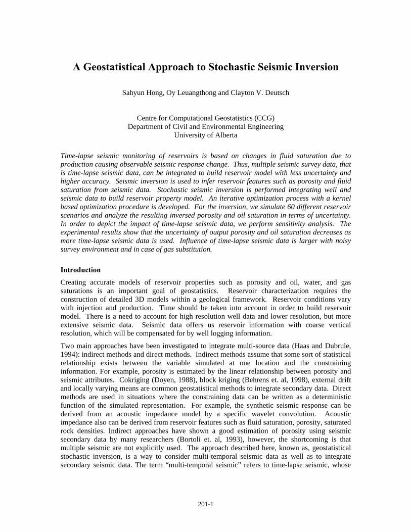
The Gassmann fluid substitution model is used to calculated the undrained bulk modulus of a fluid filled rock (KU) from the porosity (φ), the bulk modulus of the solid grains (KS), the bulk modulus of the fluid mixture occupying the pore space (KF) and the dry bulk modulus of the rock frame (KD) (Mavko et. al, 1998):

201-3

2

2

1

1

D

SU D

D

F S S

KK

K K KK K Kφ φ

⎛ ⎞−⎜ ⎟

⎝ ⎠= +−

+ +

The density of the saturated rock is given by the weighted average of the densities of the components:

(1 )o o w w g g grainS S Sρ φ ρ φ ρ φ ρ φ ρ= + + + −

where , ,o w gρ ρ ρ , and grainρ are the densities for oil, water, gas, and component grains. The compressional velocity (Vp) is then computed for an isotopic layer, elastic medium (Kennett, 1983):

43U dry

p

K GV

ρ

+=

where GDry is a shear modulus of the dry rock frame.

In order to use the Gassmann equation, we must first approximate the bulk modulus (KF) of the fluid mixture. The bulk modulus of the fluid mixtures depends on the details of the small-scale fluid distribution. If the fluids are mixed uniformly at a very fine scale, the saturation weighted harmonic average is appropriate (Mavko et. al, 1998; Bentley et. al, 1999):

1

1 g o w

F g o w

S S SK K K K

= + +

If the fluids are patchy at a scale that is smaller than the seismic wave length, but larger than the scale at which the pore scale fluids can equilibrate pressures through local flow, then the effective fluid bulk modulus is larger. The upper bound on the fluid mixture bulk modulus is the saturation weighted arithmetic average:

2F g g o o w wK S K S K S K= + +

We used the average of the uniform KF1 and patch KF2 as an effective bulk modulus of the fluid filled rock KF:

1 2

2F F

FK KK +

=

Other factors influencing the KU and Vp are fixed as a constant in the designated experiment:

- KS: the bulk modulus of the solid grains

- KD: the bulk modulus of the dry rock frame

- GDry: the same as KDry

- Reservoir temperature

201-4

- Fluids pressure

Figure 2 represents the change of bulk modulus KU of the saturated rock according to the fluid changes. We used a true porosity, initial oil saturation, and 20% changed oil saturation as input information in order to check how much difference exists in the saturated rock bulk modulus value. We set oil being replaced by water with 20% amounts that is averaged over the considered reservoir depth. Solid line and dashed line in the middle of the figure are initial oil saturation and changed oil saturation by that amount, respectively. Newly estimated bulk modulus through the Gassmann model is shown as a dashed line in the right most plot of Figure 2. The estimated bulk modulus KU, that is different from the value from initial fluid saturation, will be used to calculate seismic velocity corresponding to the change in fluid type and amounts (Kennett, 1983).

Forward Modeling

Seismic velocity for the specific reservoir conditions is estimated by using the Gassmann equation. Seismic velocity and density of saturated reservoir are used to generate acoustic impedance values. Impedance is the value of seismic velocity multiplied by density, which is a small scale feature characterizing the reservoir. However, the estimated impedances at the unsampled location should be converted into large scale seismic responses in order to compare to the true seismic response. Forward modeling represents the conversion of small scale impedance features into corresponding large scale seismic trace (Gadallah, 1994). Forward modeling is performed through convolving the specific wavelet function. Figure 3 shows forward modeling process conceptually. The estimation results from the Gassmann fluid substitution model and Kennett’s equation are used as input variables. Acoustic impedance features explicitly can be calculated by multiplication of seismic velocity and filled rock density. Acoustic impedance contrast between two distinct layers indicates seismic reflection and we can obtain continuous seismic response through convolving reflection coefficients and selected wavelet function. The choice of wavelet function is a critical issue in the field of seismic forward modeling, however, that problem is beyond the scope of this research.

Optimized Perturbation

Porosity and fluid saturation quantity at unsampled locations are generated through geostatistical simulation technique. They are used as input parameters into fluid substitution model to obtain the corresponding seismic velocity. The synthetic seismograms being generated from the fluid substitution model and forward model should now be compared with true seismic response. If there is no significant difference (e.g. RMS errors) between the true seismic and synthetic seismic, then the estimated porosity and fluid saturation quantity would be correct for the specific reservoir conditions. Otherwise, the simulated porosity and fluid saturation quantity are to be changed, which is the optimized perturbation process. It is noted that porosity and fluid saturation quantity are hardly intertwined with each other, in other words, the perturbation of porosity does not affect the perturbation of fluid saturation.

Porosity can be spatially modeled with covariance or variogram. To perturb porosity values the kernel based optimization is adopted here. The kernel comes from spatially correlated covariance function and the strength of perturbation depends on the shape of covariance function. Figure 4 is the variogram and covariance plot of the porosity. Covariance plot is renamed by weight function W(h). Fitted variogram model is a spherical model with no nugget and 3m range distance. Weight function plot is exactly the reciprocal of the spherical model with same range. As the

201-5

distance between the position to be selected and to be changed increases, the perturbation strength decreases. Figure 5 is a process of kernel based perturbation at a specific depth location. Solid line in the shaded box is one of the simulated porosities and dashed line is a resulting perturbated line. One of two dashed lines is chosen according to the sign of perturbation quantity Δ.

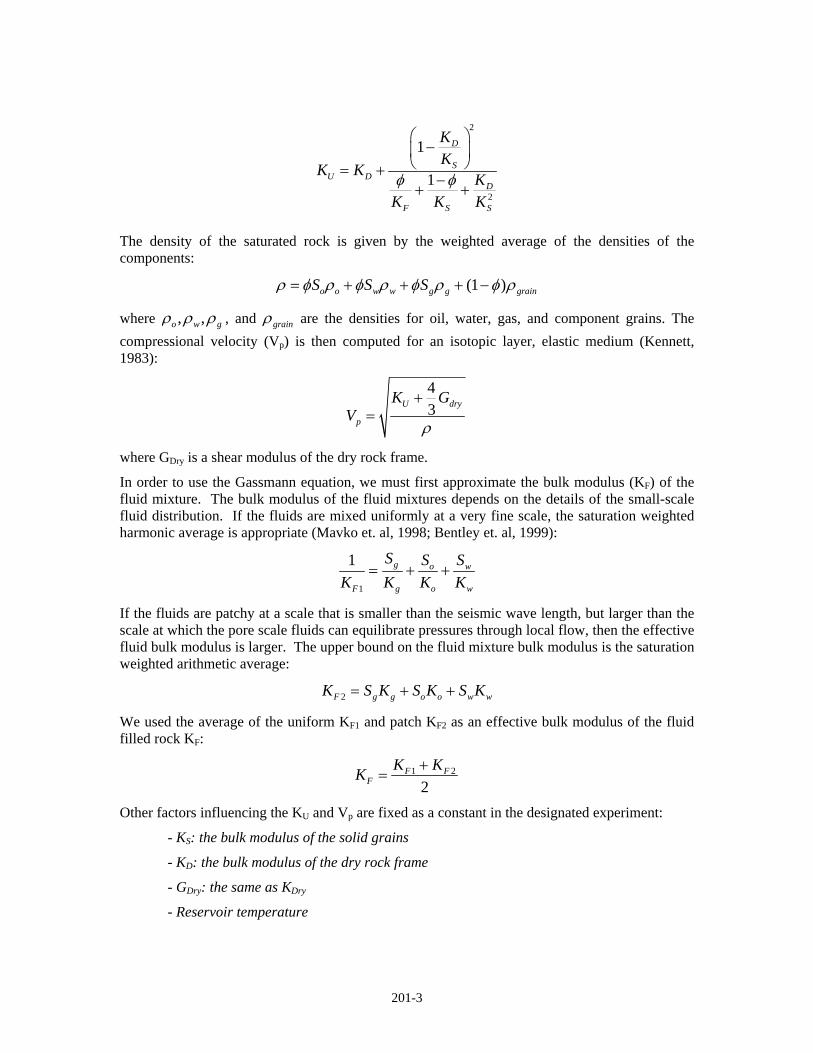
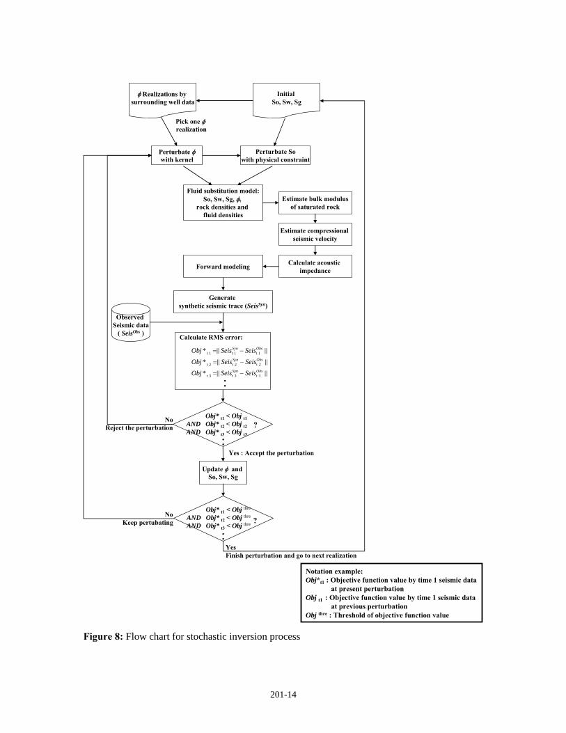
Another constraint on the fluids saturation perturbation is the consistency of changes which means physical constraint. Abrupt changes of fluids distribution, either increase or decrease, do not occur in natural reservoir conditions due to continuous distribution of geo-fluids. Figure 6 represents constraints on perturbation of fluid saturation. Perturbated values without physical constraint are shown on the left in Figure 6 and perturbated values with considering physical constraint are shown on the right in Figure 6. Those two perturbed values result in the same quality, which means they represent the same seismic response. However, we select perturbated values shown in right of the figure. Physical constraint is carried out by minimizing the variance of difference between initial saturation and perturbated saturation. Amount of saturation change (Soini – Sopert) follows more uniform distribution after applying physical constraint. Figure 8 illustrates the overall process for stochastic seismic inversion. Inversion process including optimized perturbation goes to work one porosity realization and fluid saturation at a time. RMS errors between the synthetic and observed seismic amplitudes are considered objective function. Pre-defined threshold value of objective functions is set as a stop criterion.

Seismic Data with Noise

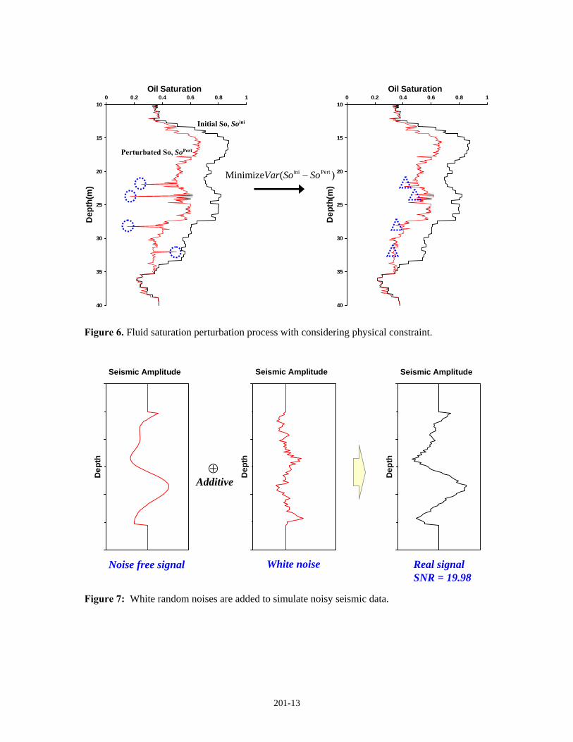
In a real seismic survey, noise is an obstacle to obtain good inversion results. Our goal is to generate realistic porosity and fluids saturation information from time lapse seismic data under time dependent reservoir conditions. Besides we need to demonstrate how fluids change and/or noise change impact on the resulting inversed porosity and fluid saturation. For example, inverted fluids saturation under high noise level seismic data would show different shape compared with true fluids saturation shape even though there is no fluid changes. White noise was added to noise-free signal shown in Figure 7 and obtained three different noisy data with different SNR levels.

Case Studies

We have tested a 2-D simulated case before proceeding 4-D real case: 1-D vertical and time dimension. Vertical dimension of test data is 100m with 0.1m interval. Porosity and fluid saturation is sampled and simulated at every 0.1m unit. Initial fluid saturation information is provided and 100 SGS realizations of porosity are prepared (Deutsch, 1992). Stochastic seismic inversion is performed for different pre-defined reservoir conditions. The following explains several reservoir scenarios that we had tested:

- Inversed porosity and oil saturation with fluids change and with different noise level

Oil is substituted by water with 5, 10, 15, 20, 25% change

201-6

Seismic time 1time 2time 3time 4

Seismic time 1time 2time 3

Seismic time 1time 2

Noise level 3Noise level 2Noise level 1

Seismic time 1

Seismic time 1time 2time 3time 4

Seismic time 1time 2time 3

Seismic time 1time 2

Noise level 3Noise level 2Noise level 1

Seismic time 1

,inv invSoφ

- Inversed porosity and oil saturation with fluids change and with different noise level

Oil is substituted by gas with 5, 10, 15, 20, 25% change

Seismic time 1time 2time 3time 4

Seismic time 1time 2time 3

Seismic time 1time 2

Noise level 3Noise level 2Noise level 1

Seismic time 1

Seismic time 1time 2time 3time 4

Seismic time 1time 2time 3

Seismic time 1time 2

Noise level 3Noise level 2Noise level 1

Seismic time 1

,inv invSoφ

A total of 120 different cases are considered for seismic inversion to estimate porosity and oil saturation (noise level × # of seismic × # of fluid change amount × # of fluid type change = 3 × 4 × 5 × 2 = 120). Figures 9 and 10 are one of the resulting inverted porosity and oil saturation with two time-lapse and three time-lapse seismic data at a specific reservoir conditions.

It is shown in Figure 9 that inverted porosity and oil saturation results when oil is substituted by water by 20%. Uncertainty is defined as an average of variance of optimized inversed value. Uncertainty in inverted porosity decreases by 7.5% when using three time-lapse seismic data. Uncertainty in inverted oil saturation decreases by 25% when using three time-lapse seismic data. Reduction in uncertainty is more obvious in case of gas substitution scenario (Figure 10). Uncertainty of inverted porosity and inversed oil saturation decreases by 19.2% and 29.1%, respectively.

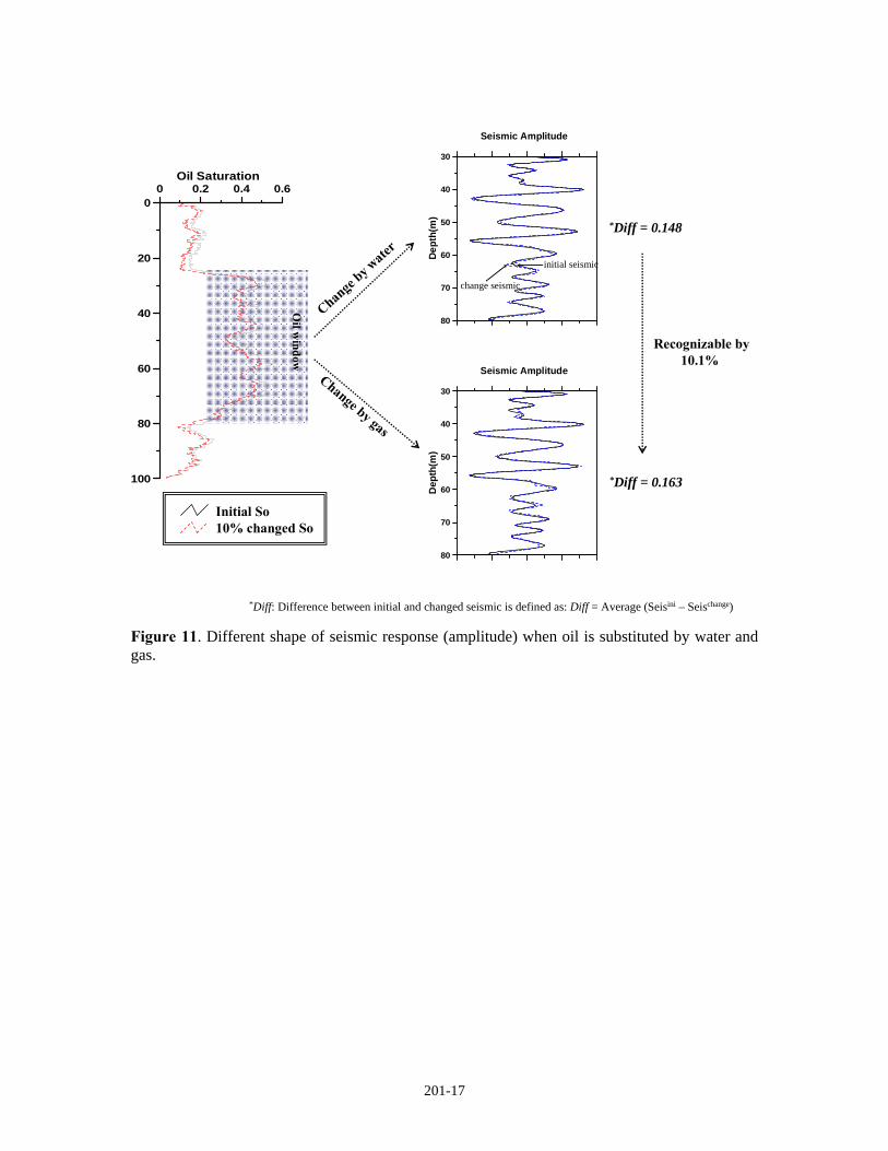
Seismic response is different for two different type of fluid injection. Figure 11 shows the seismic response pattern when oil is replaced by water and gas, respectively. Seismic difference caused by water injection is smaller than caused by gas injection. Seismic resolution increases by 10.1% when oil is substituted by gas. Thus, ‘oil by water’ change is not obvious to seismic amplitude compared to the oil by gas change. It is noted that change of fluid type (oil water or oil gas) is an important factor in seismic inversion. Especially, fluid type change is more important under noisy environment.

201-7

Evaluation of the Inversion Results

Uncertainty Assessment

Our main goal is to generate porosity and fluids saturation models with low uncertainty over the whole reservoir. Figures 12 and 13 represent the estimated uncertainty in case of several different reservoir conditions. To estimate uncertainty (U) we calculated a variance of 100 optimized perturbation values at a specific depth location. Then, we calculated an average of the variance over the whole depth (100m with 0.1m interval: total 1000 points). Uncertainty is plotted for 120 different reservoir scenarios; different noise quantity, different number of incorporated seismic data, quantity of fluid changes and fluid types. Each pixel shown in Figures 12 and 13 indicate one of 120 different scenarios. At first, Figure 10 indicates the uncertainty distribution resulted from 60 different reservoir scenarios with being substituted by water. Dominant factors over the uncertainty distribution are the number of time-lapse seismic data and quantity of additive noise. Upper picture of Figure 10 (where U and U are specified) shows a trend in uncertainty. Here, U is an average uncertainty of 20 different reservoir cases over the specific noise environment. In other words, U is an average uncertainty at a specific noise environment for an inversed porosity or inversed oil saturation. U explains that uncertainty depends on the noise level (SNRs level). Figure 13 represents the resulting uncertainty distribution over 60 different simulated reservoir scenarios under substitution by gas. Pixel grey colors are lighter than that of Figure 12, which means the overall uncertainty is lower than in case of gas substitution. This agrees with the fact that seismic response is more recognizable when oil is replaced by gas.

Sensitivity Analysis

We quantified the uncertainty under four input variables: noise amounts, number of seismic, changed fluids type, fluid change amount. In this section, we observe the contribution of time-lapse seismic data number to the uncertainty reduction. Estimated uncertainty maps, Figures 12 and 13 are used to create an uncertainty vector map. Figures 14 and 15 are the uncertainty vector maps. The decrement vector of the uncertainty is represented by arrows that have quantity and direction. Figure 14 is the resulting uncertainty vector map in case of being substituted by water. We can observe a large contribution of seismic data number when performing oil saturation inversion since the magnitude of arrow is larger than when performing porosity inversion. Figure 15 is an uncertainty vector map with the case of gas substitution. In this case, the effect of seismic data is more obvious compared with substitution by water. Furthermore, the amounts of fluid change and number of seismic data have large influence on uncertainty decrease (the vector points steeply toward the south-east direction) and that influence is getting larger with higher noise. Figure 16 represents the reduction in uncertainty according to the number of time-lapse seismic data. Uncertainty shown in this figure is an average of the uncertainty resulting from five different amounts of fluid change. For example, plotted uncertainty of one time-lapse seismic data under lowest noise (solid line in figure 16) level is an average value of uncertainty coming from 5, 10, 15, 20, 25% fluid change under the lowest noise level. A greater reduction in uncertainty is seen when oil is replaced by gas.

Conclusions

Reservoir characterization with time-lapse seismic data is reviewed. For simplicity, 2-D case is described and analyzed but 4-D real case is a fairly straightforward extension of dimensionality. Simulated reservoir conditions such as fluid changes, fluid type change and noise change are used to test the effect of incorporating time-lapse seismic data. We have the following comments from

201-8

the analysis: (1) time-lapse seismic data is useful when we need to build a time varying reservoir model in terms of uncertainty; (2) as the number of adopted seismic data increases, the uncertainty of porosity and oil saturation decreases; (3) oil by gas change case shows that the type of fluid change is discernible to seismic amplitude trace and this results in more steep reduction in uncertainty of porosity and oil saturation; and (4) the uncertainty reduction effect of time-lapse seismic data gets larger under noisy environment.

It is widely accepted that more information would be useful to obtain the desired results; many secondary data would reduce risks and improve target accuracies. This study quantitatively shows that integration of multiple seismic data based on the developed method can be considered desirable in terms of reducing uncertainties. One could also observe the trend of reduction in uncertainties when multiple seismic data is used under different fluid types and noise contents.

Future Work

The proposed framework contains several sequential steps for stochastic inversion such as simulation of primary data, fluids substitution, forward modeling, optimized perturbation, and noise embedment, which requires many parameters for the specific step. These user-defined parameters could invoke variation in the final uncertainty; therefore we need to describe uncertainty propagation during the whole stochastic inversion process.

Another aspect to be considered is to model noise impact. Realistic geological and geophysical data is usually disturbed by multiplicative noise even though we have only managed with additive type of noise. Multiplicative noises are to be considered and uncertainty analysis will be addressed as specified above.

References

Behrens, R.A., MacLeod, M.K., Tran, T.T., and Alimi, A.O., 1998, Incorporating seismic attribute maps in 3D reservoir models; SPE Reservoir and Engineering, Apr, 122-126

Bortoli, L.J., Alabert, F., Haas, A. and Journel, A., 1993, Constraining stochastic images to seismic data: Stochastic simulation of synthetic seismograms; Geostatistics Tróia 92 proceeding, 4th International Geostatistics Congress, Kluwer Academic Publishers

Doyen, P.M., 1988, Porosity from seismic data: A geostatistical approach: Geophysics; 53, 1263-1275

Deutsch, C.V. and Journel, A.G., 1992, GSLIB: Geostatistical software library and user’s guide; Oxford University Press, New York, NY

Gadallah, M.R., 1994, Reservoir seismology: geophysics in nontechnical language; PennWell Books, Tulsa, Okla

Haas, A and Dubrule O., 1994, Geostatistical inversion-a sequential method of stochastic reservoir modeling constrained by seismic data: First Break, 12, 561-569

Kennett, B.L., 1983, Seismic wave propagation in stratified media; Cambridge University Press, NY

Lumley, D.E., 2001, Time-lapse seismic reservoir monitoring: Geophysics, 66, 50-53

201-9

Mavko, G., Mukerji, T., and Dvorkinm J., 1998, The rock physics handbook: Tools for seismic analysis in porous media; Cambridge University Press, Cambridge, United Kingdom

Vasco, D.W., Datta-Gupta, A., Behrens, R., Condon, P., and Rickett, J., 2004, Seismic imaging of reservoir flow properties: Time-lapse amplitude change; Geophysics, 69, 14251442

201-10

8

6

4

2

0

Dept

h(m

)

Porosity

8

6

4

2

0

Dept

h(m

)

So

8

6

4

2

0

Dept

h(m

)

Ip

+

Res

ervo

ir

8

6

4

2

0

Dept

h(m

)

Seismic Amplitude

8

6

4

2

0

Dept

h(m

)

Ip

8

6

4

2

0

Dept

h(m

)

Porosity

8

6

4

2

0

Dept

h(m

)

So

Earth modelof acousticimpedance

Inputwavelet

SeismicTrace

Real porosity andfluid saturation

Established modelof acousticimpedance

EstimatedwaveletInversed porosity and

fluid saturation

8

6

4

2

0

Dept

h(m

)

Seismic Amplitude

SeismicTrace

Forward modeling

Inverse modeling

8

6

4

2

0

Dept

h(m

)

Porosity

8

6

4

2

0

Dept

h(m

)

So

8

6

4

2

0

Dept

h(m

)

Ip

+

Res

ervo

ir

8

6

4

2

0

Dept

h(m

)

Seismic Amplitude

8

6

4

2

0

Dept

h(m

)

Ip

8

6

4

2

0

Dept

h(m

)

Porosity

8

6

4

2

0

Dept

h(m

)

So

Earth modelof acousticimpedance

Inputwavelet

SeismicTrace

Real porosity andfluid saturation

Established modelof acousticimpedance

EstimatedwaveletInversed porosity and

fluid saturation

8

6

4

2

0

Dept

h(m

)

Seismic Amplitude

SeismicTrace

Forward modeling

Inverse modeling

8

6

4

2

0

Dept

h(m

)

Porosity

8

6

4

2

0

Dept

h(m

)

So

8

6

4

2

0

Dept

h(m

)

Ip

+

Res

ervo

ir

8

6

4

2

0

Dept

h(m

)

Seismic Amplitude

8

6

4

2

0

Dept

h(m

)

Ip

8

6

4

2

0

Dept

h(m

)

Porosity

8

6

4

2

0

Dept

h(m

)

So

Earth modelof acousticimpedance

Inputwavelet

SeismicTrace

Real porosity andfluid saturation

Established modelof acousticimpedance

EstimatedwaveletInversed porosity and

fluid saturation

8

6

4

2

0

Dept

h(m

)

Seismic Amplitude

SeismicTrace

Forward modeling

Inverse modeling

Figure 1. Schematic overview of forward modeling and inverse modeling.

201-11

2000 4000 6000

Bulk modulus ofthe saturated rock(KU)

(MPa)

52

48

44

40

36

32

28

Dep

th (m

)

0.3 0.4 0.5 0.6

Oil Saturation (So)

52

48

44

40

36

32

28

Dep

th (

m)

0 0.1 0.2 0.3 0.4 0.5

Porosity

52

48

44

40

36

32

28

Dep

th (

m)

Initial SoChanged So by 20%Initial SoChanged So by 20%

Initial KUChanged KU

Initial KUChanged KU

Move to forward modeling to generate synthetic seismic trace

Figure 2. Illustration of estimated bulk modulus of the saturated rock through the Gassmann fluid substitution model.

ρV(t) R(t)

Impedance Reflection Coefficient

R1

R2

R3

R4

R5

2 1

2 1

( )( )Ip IpRIp Ip

−=

+

S(t)

Convolution bywavelet function b(t)

S(t) = R(t) * b(t)

Gassmann fluid substitution model

Compressional seismic velocity (Vp)&

Density of the saturated rock (Kennett, 1983)

FluidsPorosity

Rock density

Figure 3. Illustration of forward modeling. Wavelet convolution is a process for performing forward modeling

201-12

γ(h)

W(h

)

0 1 2 3 4Distance

0

0.2

0.4

0.6

0.8

1

0 1 2 3 4Distance

0

0.2

0.4

0.6

0.8

1

Figure 4. Variogram function and weight function of the porosity. Weight function is an exact reciprocal function of the variogram.

40

30

20

10

35

25

15

Dep

th

0 0.2 0.4 0.6 0.8 1Porosity Δ

+Δ-Δ

Weight functionPerturbation area

10

5

15 Figure 5. Kernel based porosity perturbation. Kernel comes from the spatial model of porosity.

201-13

40

30

20

10

35

25

15

Dep

th(m

)0 0.2 0.4 0.6 0.8 1

Oil Saturation

40

30

20

10

35

25

15

Dep

th(m

)

0 0.2 0.4 0.6 0.8 1Oil Saturation

Initial So, Soini

Perturbated So, SoPert

ini PertMinimize ( )Var So So−

Figure 6. Fluid saturation perturbation process with considering physical constraint.

Dep

th

Seismic Amplitude

Dep

th

Seismic Amplitude

Noise free signal White noise

⊕Additive

Dep

th

Seismic Amplitude

Real signalSNR = 19.98

Figure 7: White random noises are added to simulate noisy seismic data.

201-14

φ Realizations by surrounding well data

Perturbate Sowith physical constraint

Generate synthetic seismic trace (SeisSyn)

Estimate bulk modulusof saturated rock

Estimate compressionalseismic velocity

Calculate acoustic impedance

Fluid substitution model:So, Sw, Sg, φ,

rock densities and fluid densities

Calculate RMS error:

t 1 t 1 t 1

t 2 t 2 t 2

t 3 t 3 t 3

*

*

*

Syn Obs

Syn Obs

Syn Obs

Obj Seis Seis

Obj Seis Seis

Obj Seis Seis

= −

= −

= −

?Obj* t1 < Obj t1

AND Obj* t2 < Obj t2AND Obj* t3 < Obj t3

Observed Seismic data

( SeisObs )

Forward modeling

Pick one φrealization

Initial So, Sw, Sg

Perturbate φwith kernel

Yes : Accept the perturbation

NoReject the perturbation

Obj* t1 < Obj thre

AND Obj* t2 < Obj thre

AND Obj* t3 < Obj thre

Update φ and So, Sw, Sg

NoKeep pertubating ?

YesFinish perturbation and go to next realization

Notation example: Obj*t1 : Objective function value by time 1 seismic data

at present perturbationObj t1 : Objective function value by time 1 seismic data

at previous perturbationObj thre : Threshold of objective function value

Figure 8: Flow chart for stochastic inversion process

201-15

= 0.0792σ = 0.0592σ

2 Time-lapse Seismic data

3 Time-lapse Seismic data

: P90 – P10 interval

: True porosity

: True oil saturation

100

80

60

40

20

0

Dep

th(m

)

0 0.1 0.2 0.3 0.4Porosity

100

80

60

40

20

0

Dep

th(m

)

0 0.1 0.2 0.3 0.4Porosity

Inversed porosity and oil saturation with 2 time-lapse and with 3 time-lapse - oil by water 20%

= 0.053 = 0.0492σ 2σ

100

80

60

40

20

0

Dep

th(m

)

0 0.2 0.4 0.6Oil Sat

100

80

60

40

20

0

Dep

th(m

)

0 0.2 0.4 0.6Oil Sat

Figure 9. Inversed porosity and oil saturation with two time-lapse seismic data and 3 time-lapse seismic data in case of oil being replaced by water by 20% change.

201-16

= 0.0552σ = 0.0392σ

2 Time-lapse Seismic data

3 Time-lapse Seismic data

: P90 – P10 interval

: True porosity

: True oil saturation

Inversed porosity and oil saturation with 2 time-lapse and with 3 time-lapse- oil by gas 20%

100

80

60

40

20

0

Dep

th(m

)

0 0.1 0.2 0.3 0.4Porosity

100

80

60

40

20

0

Dep

th(m

)

0 0.1 0.2 0.3 0.4Porosity

= 0.052 = 0.0422σ 2σ

100

80

60

40

20

0

Dep

th(m

)

0 0.2 0.4 0.6Oil Sat

100

80

60

40

20

0

Dep

th(m

)

0 0.2 0.4 0.6Oil Sat

Figure 10. Inversed porosity and oil saturation with two time-lapse seismic data and 3 time-lapse seismic data in case of oil being replaced by gas by 20% change.

201-17

100

80

60

40

20

00 0.2 0.4 0.6

Oil Saturation

80

70

60

50

40

30

Dep

th(m

)

Seismic Amplitude

80

70

60

50

40

30

Dept

h(m

)

Seismic Amplitude

Oil w

indow

Initial So10% changed So

Change

by wate

r

Change by gas

*Diff = 0.148

initial seismic

*Diff = 0.163

change seismic

Recognizable by10.1%

*Diff: Difference between initial and changed seismic is defined as: Diff = Average (Seisini – Seischange) Figure 11. Different shape of seismic response (amplitude) when oil is substituted by water and gas.

201-18

1 2 3 4

252015105

Inversed Porosity Inversed Oil Saturation

- Estimated uncertainty when oil is replaced by water

Additive w

hite Noise increase

20%

30%

U

Am

ount

of

fluid

cha

nge

# of Time-lapseseismic

U

UU

U

U More Noisy

Less Noisy

Figure 12. Uncertainty distribution over 60 different simulated reservoir scenarios under the assumption oil is substituted by water. Main trend of the uncertainty distribution is summarized in the upper part. The definition of uncertainty is described in the context.

201-19

1 2 3 4

252015105

Inversed Porosity Inversed Oil SaturationA

dditive white N

oise increase

- Estimated uncertainty when oil is replaced by gas

U

Am

ount

of

fluid

cha

nge

# of Time-lapseseismic

U

UU

U

U More Noisy

Less Noisy

20%

30%

Figure 13. Uncertainty distribution over 60 different simulated reservoir scenarios under the assumption oil is substituted by gas. A trend of the uncertainty distribution is summarized in the upper part of the picture.

201-20

Inversed Porosity Inversed Oil Saturation

- Uncertainty vector map when oil is substituted by waterA

mou

nt o

f flu

id c

hang

e

# of Time-lapseseismic

Additive w

hite Noise increase

20%

30%

Figure 14. Uncertainty vector map in case of oil being substituted by water.

201-21

Inversed Porosity Inversed Oil Saturation

- Uncertainty vector map when oil is substituted by gasA

mou

nt o

f flu

id c

hang

e

# of Time-lapseseismic

Additive w

hite Noise increase

20%

30%

Figure 15. Uncertainty vector map in case of oil being substituted by gas.

201-22

0 1 2 3 4 5Number of Seismic data

0

0.1

0.2

0.3

0.4

0.5

Unc

erta

inty

SNR = 35.1SNR = 28.1SNR = 19.7

Inversed oil saturation

Oil is changed by water

Oil is changed by gas

0 1 2 3 4 5Number of Seismic data

0

0.1

0.2

0.3

0.4

0.5

Unc

erta

inty

Figure 16. The contribution of time-lapse seismic data to total uncertainty.