Fishery Data Series No. 19-21 Inriver Abundance of Kuskokwim River Chinook Salmon, 2017 by Joshua N. Clark and Nicholas J. Smith August 2019 Alaska Department of Fish and Game Divisions of Sport Fish and Commercial Fisheries
Transcript
Fishery Data Series No. 19-21
Inriver Abundance of Kuskokwim River Chinook Salmon, 2017
by
Joshua N. Clark
and
Nicholas J. Smith
August 2019
Alaska Department of Fish and Game Divisions of Sport Fish and Commercial Fisheries
Symbols and Abbreviations The following symbols and abbreviations, and others approved for the Système International d'Unités (SI), are used without definition in the following reports by the Divisions of Sport Fish and of Commercial Fisheries: Fishery Manuscripts, Fishery Data Series Reports, Fishery Management Reports, and Special Publications. All others, including deviations from definitions listed below, are noted in the text at first mention, as well as in the titles or footnotes of tables, and in figure or figure captions. Weights and measures (metric) centimeter cm deciliter dL gram g hectare ha kilogram kg kilometer km liter L meter m milliliter mL millimeter mm
Weights and measures (English) cubic feet per second ft3/s foot ft gallon gal inch in mile mi nautical mile nmi ounce oz pound lb quart qt yard yd
Time and temperature day d degrees Celsius °C degrees Fahrenheit °F degrees kelvin K hour h minute min second s
Physics and chemistry all atomic symbols alternating current AC ampere A calorie cal direct current DC hertz Hz horsepower hp hydrogen ion activity pH (negative log of) parts per million ppm parts per thousand ppt,
‰ volts V watts W
General Alaska Administrative Code AAC all commonly accepted abbreviations e.g., Mr., Mrs.,
AM, PM, etc.all commonly accepted professional titles e.g., Dr., Ph.D.,
R.N., etc.at @compass directions:
east E north N south S west W
copyright corporate suffixes:
Company Co. Corporation Corp. Incorporated Inc. Limited Ltd.
District of Columbia D.C.et alii (and others) et al.et cetera (and so forth) etc. exempli gratia (for example) e.g.Federal Information Code FIC id est (that is) i.e.latitude or longitude lat or longmonetary symbols (U.S.) $, ¢ months (tables and
figures): first three letters Jan,...,Dec registered trademark trademark United States
(adjective) U.S. United States of America (noun) USA U.S.C. United States
Code U.S. state use two-letter
abbreviations (e.g., AK, WA)
Mathematics, statistics all standard mathematical signs, symbols and abbreviations alternate hypothesis HA base of natural logarithm e catch per unit effort CPUE coefficient of variation CV common test statistics (F, t, χ2, etc.) confidence interval CI correlation coefficient (multiple) R correlation coefficient (simple) r covariance cov degree (angular ) ° degrees of freedom df expected value E greater than > greater than or equal to ≥ harvest per unit effort HPUE less than < less than or equal to ≤ logarithm (natural) ln logarithm (base 10) log logarithm (specify base) log2, etc. minute (angular) ' not significant NS null hypothesis HO percent % probability P probability of a type I error (rejection of the null hypothesis when true) α probability of a type II error (acceptance of the null hypothesis when false) β second (angular) " standard deviation SD standard error SE variance
population Var sample var
FISHERY DATA SERIES NO. 19-21
INRIVER ABUNDANCE AND RUN TIMING OF KUSKOKWIM RIVER CHINOOK SALMON, 2017
by Joshua N. Clark and Nicholas J. Smith
Alaska Department of Fish and Game, Division of Commercial Fisheries, Anchorage
This report was prepared by the Alaska Department of Fish and Game, Division of Commercial Fisheries, under Pacific States Marine Fisheries Commission Award Number 17-91G.
Alaska Department of Fish and Game Division of Sport Fish, Research and Technical Services 333 Raspberry Road, Anchorage, Alaska, 99518-1565
August 2019
ADF&G Fishery Data Series was established in 1987 for the publication of Division of Sport Fish technically oriented results for a single project or group of closely related projects, and in 2004 became a joint divisional series with the Division of Commercial Fisheries. Fishery Data Series reports are intended for fishery and other technical professionals and are available through the Alaska State Library and on the Internet: http://www.adfg.alaska.gov/sf/publications/. This publication has undergone editorial and peer review.
Joshua N. Clark and Nicholas J. Smith, Alaska Department of Fish and Game, Division of Commercial Fisheries,
333 Raspberry Road, Anchorage AK, 99518, USA
This document should be cited as follows: Clark, J. N., and N. J. Smith. 2019. Inriver abundance and run timing of Kuskokwim River Chinook salmon, 2017.
Alaska Department of Fish and Game, Fishery Data Series No. 19-21, Anchorage.
The Alaska Department of Fish and Game (ADF&G) administers all programs and activities free from discrimination based on race, color, national origin, age, sex, religion, marital status, pregnancy, parenthood, or disability. The department administers all programs and activities in compliance with Title VI of the Civil Rights Act of 1964, Section 504 of the Rehabilitation Act of 1973, Title II of the Americans with Disabilities Act (ADA) of 1990, the Age Discrimination Act of 1975, and Title IX of the Education Amendments of 1972.
If you believe you have been discriminated against in any program, activity, or facility please write: ADF&G ADA Coordinator, P.O. Box 115526, Juneau, AK 99811-5526
U.S. Fish and Wildlife Service, 4401 N. Fairfax Drive, MS 2042, Arlington, VA 22203 Office of Equal Opportunity, U.S. Department of the Interior, 1849 C Street NW MS 5230, Washington DC 20240
The department’s ADA Coordinator can be reached via phone at the following numbers: (VOICE) 907-465-6077, (Statewide Telecommunication Device for the Deaf) 1-800-478-3648,
(Juneau TDD) 907-465-3646, or (FAX) 907-465-6078 For information on alternative formats and questions on this publication, please contact:
ADF&G, Division of Sport Fish, Research and Technical Services, 333 Raspberry Rd, Anchorage AK 99518 (907) 267-2375
LIST OF TABLES ......................................................................................................................................................... ii
LIST OF FIGURES ....................................................................................................................................................... ii
LIST OF APPENDICES ............................................................................................................................................... ii
Study Area ..................................................................................................................................................................... 3 Mark–Recapture Abundance Estimation ....................................................................................................................... 4
First Event Sampling ................................................................................................................................................ 4 Telemetry Tracking .................................................................................................................................................. 5 Harvest Mortality ...................................................................................................................................................... 6 Second Event Sampling Methods ............................................................................................................................. 6 Data Analysis ............................................................................................................................................................ 7
Run Timing .................................................................................................................................................................... 9 Migration Rate ............................................................................................................................................................... 9
TABLES AND FIGURES ........................................................................................................................................... 15
APPENDIX A: STATISTICAL TESTS FOR ANALYZING DATA FOR SEX AND SIZE BIAS .......................... 29
ii
LIST OF TABLES Table Page 1 Summary of aerial telemetry tracking surveys used to locate radiotagged Chinook salmon in the
Kuskokwim River, 2017. ............................................................................................................................... 16 2 Monitored and unmonitored Chinook salmon spawning tributaries located within each of the subareas
used to classify the final location of radiotagged fish in the Kuskokwim River, 2017. ................................ 16 3 Operational periods and inoperable days at Kuskokwim Area weir projects, 2017. ..................................... 17 4 The 9 mutually exclusive classes used to separate radiotagged Kuskokwim River Chinook salmon for
variance estimation, 2017. ............................................................................................................................. 17 5 Kuskokwim River Chinook salmon abundance estimate worksheet, 2017. .................................................. 17 6 Tagged and untagged Kuskokwim River Chinook salmon captured by day at the rkm 67 tagging site,
2017. .............................................................................................................................................................. 18 7. Fates assigned to Chinook salmon radiotagged in the Kuskokwim River, 2017. .......................................... 19 8 Confirmed reports of tagged Kuskokwim River Chinook salmon harvested in the subsistence fishery,
2017. .............................................................................................................................................................. 19 9 Number of spaghetti tagged Kuskokwim River Chinook salmon considered part of the marked (M′)
population for abundance estimation, 2017. .................................................................................................. 19 10 Number of tagged Kuskokwim River Chinook salmon observed at each upriver recapture site and
considered part of capture (C) and recapture (R') populations for abundance estimation, 2017. .................. 20 11 Kuskokwim River Chinook salmon radio tag recovery ratios by location, 2017. ......................................... 21 12 Temporal recovery ratios of radiotagged Kuskokwim River Chinook salmon, 2017. .................................. 21 13 Number of length samples available from each recapture location used to test for sampling bias of
Kuskokwim River Chinook salmon, 2017. ................................................................................................... 22 14 Results of tests for size selective sampling in the marked (M), captured (C), and recaptured (R) sample
populations of Kuskokwim River Chinook salmon using the Kolmogorov-Smirnov test (D), 2017. ........... 22 15 Median tag deployment date at rkm 67 for Kuskokwim River Chinook salmon migrating to known
subarea, 2017. ................................................................................................................................................ 23 16 Median travel time (days; IQR) and migration rate (km/day; IQR) between each successive mainstem
telemetry towers for Chinook salmon tracked to subareas 2 (lower river tributaries), 4 (middle Kuskokwim River), and 5 (headwaters), 2017. ............................................................................................. 23
LIST OF FIGURES Figure Page 1 Location of the tagging site, telemetry towers, and escapement monitoring weirs used to tag, track, and
recapture Kuskokwim River Chinook salmon, 2017. .................................................................................... 24 2 Location of Kuskokwim River Chinook salmon tagging sites, drift zones, and field camp, 2017. ............... 25 3 Subareas used to classify the final location of radiotagged Chinook salmon in the Kuskokwim River,
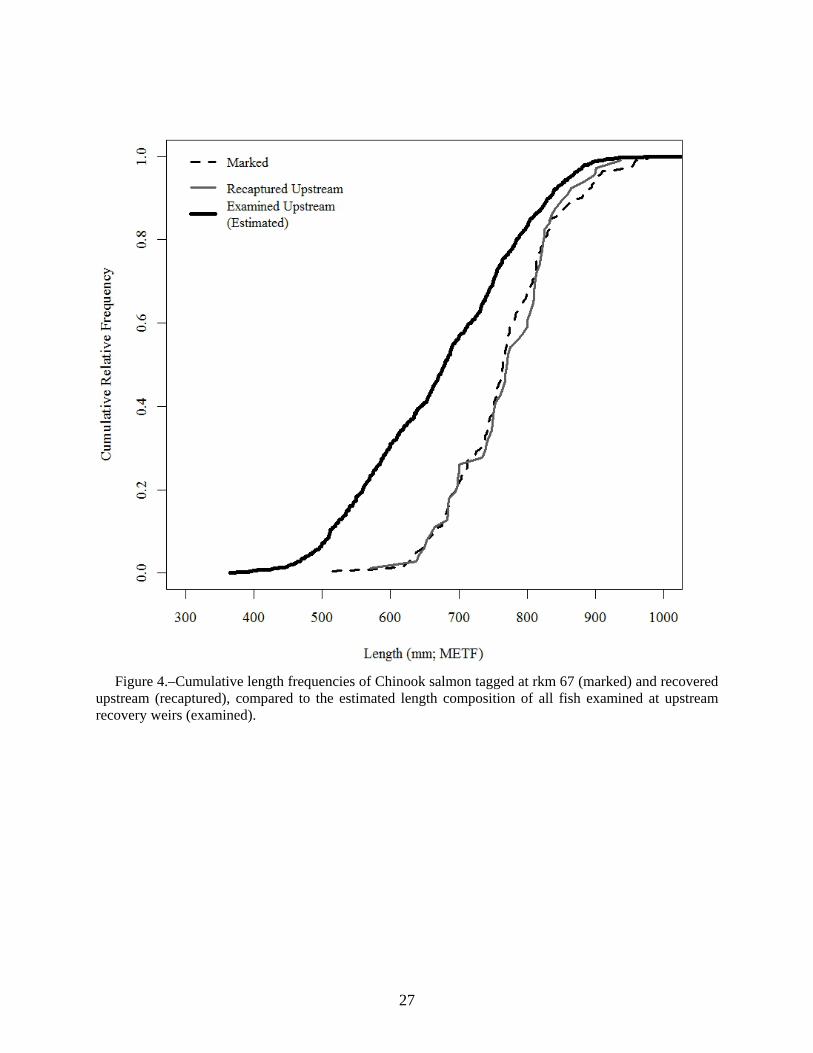
2017. .............................................................................................................................................................. 26 4 Cumulative length frequencies of Chinook salmon tagged at rkm 67 and recovered upstream,
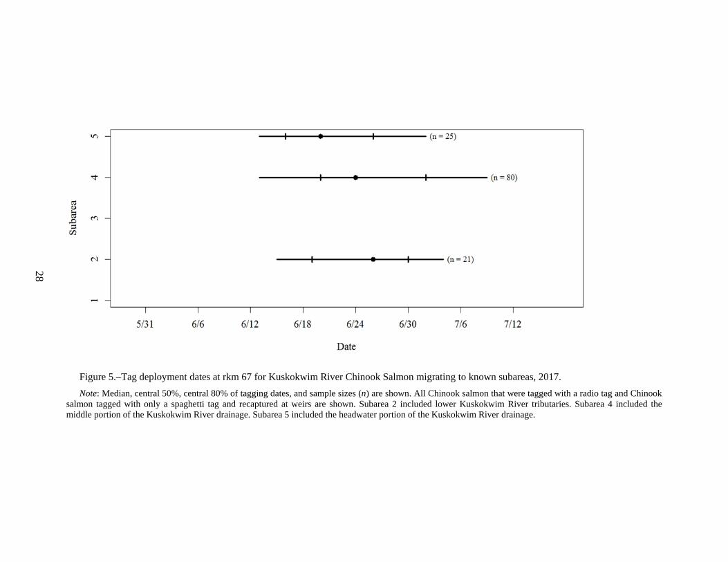
compared to the estimated length composition of all fish examined at upstream recovery weirs. ................ 27 5 Tag deployment dates at rkm 67 for Kuskokwim River Chinook Salmon migrating to known subareas,
LIST OF APPENDICES Appendix Page A1 Tests of consistency for the Petersen estimator. ............................................................................................ 30 A2 Detection of size and/or sex selective sampling (from Stuby 2007). ............................................................ 31
1
ABSTRACT A 2-sample mark–recapture experiment was conducted to estimate the abundance of adult Chinook salmon Oncorhynchus tshawytscha returning to the Kuskokwim River in 2017. Tagging occurred downriver from all known spawning tributaries, except the Eek River. All fish were marked with a dorsally attached spaghetti tag, and a subset of spaghetti tagged fish was also fitted with a radio tag to evaluate assumptions of the abundance estimator and monitor upriver movement. Radiotagged fish were tracked throughout the study area using a network of telemetry stations and a series of aerial telemetry surveys. A total of 8 escapement monitoring weirs were operated upriver from the tag site and served as recapture locations for tagged fish. Inriver abundance of Chinook salmon upstream of rkm 67 in 2017 was 125,339 fish (95% CI: 95,954–149,842). Radiotagged Chinook salmon traveling to upriver tributaries were captured and tagged earlier in the run compared to tagged fish migrating to middle river tributaries. Chinook salmon returning to lower river tributaries were captured and tagged throughout the entire run. Chinook salmon swam at a median speed of 46 rkm/day (range: 38–54 rkm/day) through all portions of the mainstem Kuskokwim River upstream from Bethel.
INTRODUCTION Alaska Department of Fish and Game (ADF&G) fisheries managers require accurate estimates of Chinook salmon Oncorhynchus tshawytscha abundance and detailed information about fish migration as they pass through harvest areas to manage subsistence and commercial fisheries within the Kuskokwim River. The Kuskokwim River supports a run of Chinook salmon that averages nearly 240,000 fish (Smith and Liller 2018). Historically, annual run sizes have been adequate to support an unrestricted subsistence fishery. The Kuskokwim River subsistence fishery is one of the largest in Alaska, accounts for 50% or more of the statewide subsistence harvest of Chinook salmon (Fall et al. 2015), and harvests an average of 30% of the total annual run (range: 8–56%; Smith and Liller 2018). Since 1985, there has been no directed commercial fishery for Kuskokwim River Chinook salmon, but incidental harvest has occurred during chum O. keta, sockeye O. nerka, and coho O. kisutch salmon fisheries.
Total annual abundance of Kuskokwim River Chinook salmon has been estimated using a statistical run reconstruction model that used previously defined relationships between total abundance and indices of abundance from a range of monitoring projects (Bue et al. 2012; Smith and Liller 2018). Accurate abundance estimates required that the run reconstruction model was scaled appropriately. The run reconstruction model had been scaled using estimates of total run size from 2003 to 2007, a period of average and record high returns (Bue et al. 2012; Schaberg et al. 2012). Since 2010, annual Chinook salmon run size has been below average, including record low run sizes in 2010, 2012, and 2013 (Smith and Liller 2018). In 2013, it was recommended that additional independent estimates of total abundance be collected to evaluate model performance in low abundance years (ADF&G 2013). These estimates would also be used to rescale the model for improved abundance estimation. With this recommendation, a 3-year mark–recapture study was initiated by ADF&G from 2014 and 2016 to estimate the annual abundance of Kuskokwim River Chinook salmon (Head et al. 2017; Smith and Liller 2017a and 2017b).
The mark–recapture studies conducted from 2014 to 2016 provided new information to assess the Chinook salmon run reconstruction model and evaluate Chinook salmon migration characteristics. A direct comparison between the mark–recapture and run reconstruction model estimates of total run abundance illustrated that the estimates from the mark–recapture studies were, on average, 31% smaller (approximately 48,000 fish) compared to the estimates based on
2
the run reconstruction model (Liller 2017). This finding provided substantial evidence that the run reconstruction model needed to be revised to improve performance – especially during years of low run abundance. The 2015 and 2016 studies years represented the first time that tagging efforts were successfully conducted near the mouth of the Kuskokwim River and substock-specific entrance timing and migration rates were calculated as fished passed through the lower portion of Kuskokwim River (Smith and Liller 2017a and 2017b). A general pattern emerged that upriver spawning fish entered the river first, followed by middle and lower river fish entering the river later in the season at generally the same time. Swim speeds throughout the mainstem Kuskokwim River did not differ among upriver, middle river, and lower river substocks.
The success of the Chinook salmon mark–recapture program has been due, in part, to the exhaustive efforts to refine capture and tagging techniques, ability to evaluate large numbers of fish for tags near the spawning grounds, and incorporation of radiotelemetry techniques as the primary tag or for the purpose of testing model assumptions (e.g., Stuby 2007; Schaberg et al. 2010; Head et al. 2017; Smith and Liller 2017a and 2017b). The ability to use the Kuskokwim Area weir program to recapture tagged fish proved to be a notable strength of the Kuskokwim River mark–recapture study design. Recapture sites have been spatially diverse representing lower river tributaries, both north and south draining tributaries in the middle river, and a headwaters tributary. The combination of these weirs provided an opportunity to inspect thousands of fish for tags (which increased precision) and evaluate spatial and temporal assumptions of the mark–recapture estimator. The use of radiotelemetry techniques has provided opportunities to evaluate handling effects, track fish movement, determine final fate of tagged fish, test critical assumptions of the mark–recapture estimator, and in some cases create an unbiased estimate when other methods did not work (e.g., Smith and Liller 2017b). The basic study design and infrastructure was used again in 2017 with expectations of continued success.
The Pacific States Marine Fisheries Commission, in coordination with Bering Sea Fishermen’s Association, funded the mark–recapture study in 2017 because they identified the value of the project to ongoing efforts to evaluate the performance of the Chinook salmon run reconstruction model. Funding in 2017 was expected to provide 4 consecutive years (2014–2017) of independent total run abundance estimates which could be used to evaluate and improve the run reconstruction model. Due to funding limits, a modified mark–recapture study design was developed in 2017 which attempted to maintain aspects of the program that were proven successful from past studies, but also reduced total project costs. Study design changes in 2017 included: 1) utilizing a single sampling crew instead of the 2 crews used in 2015 and 2016, 2) using less expensive external tags as the primary tag instead of relying on expensive radio tags, 3) deploying only the minimum number of radio tags required to test critical mark–recapturemodel assumptions instead of the required amount needed to estimate abundance, and 4)streamlining the ground-based and aerial tracking efforts such that the combined information wasadequate to determine final fate at a broad geographic scale instead of the more intensivetracking efforts conducted in past years. This report documents the activities and results of themark–recapture study in 2017.
3
OBJECTIVES 1. Estimate the abundance of adult Chinook salmon in the Kuskokwim River for all waters
upriver of rkm 67, such that the bounds of the 95% confidence interval are within ±25% of the estimated abundance.
2. Evaluate the stock-specific run timing of Chinook salmon migrating past the Lower Kuskokwim River tag site located at rkm 67.
3. Evaluate the stock-specific migration speed of Chinook salmon traveling from rkm 67 to rkm 753.
METHODS STUDY AREA Estimates of abundance included all waters upriver of rkm 67 (Figure 1). The study encompassed an area draining approximately 108,000 km2. Due to the migratory nature of Chinook salmon, sampling and tracking efforts encompassed the entire Kuskokwim River drainage upriver from the tag site.
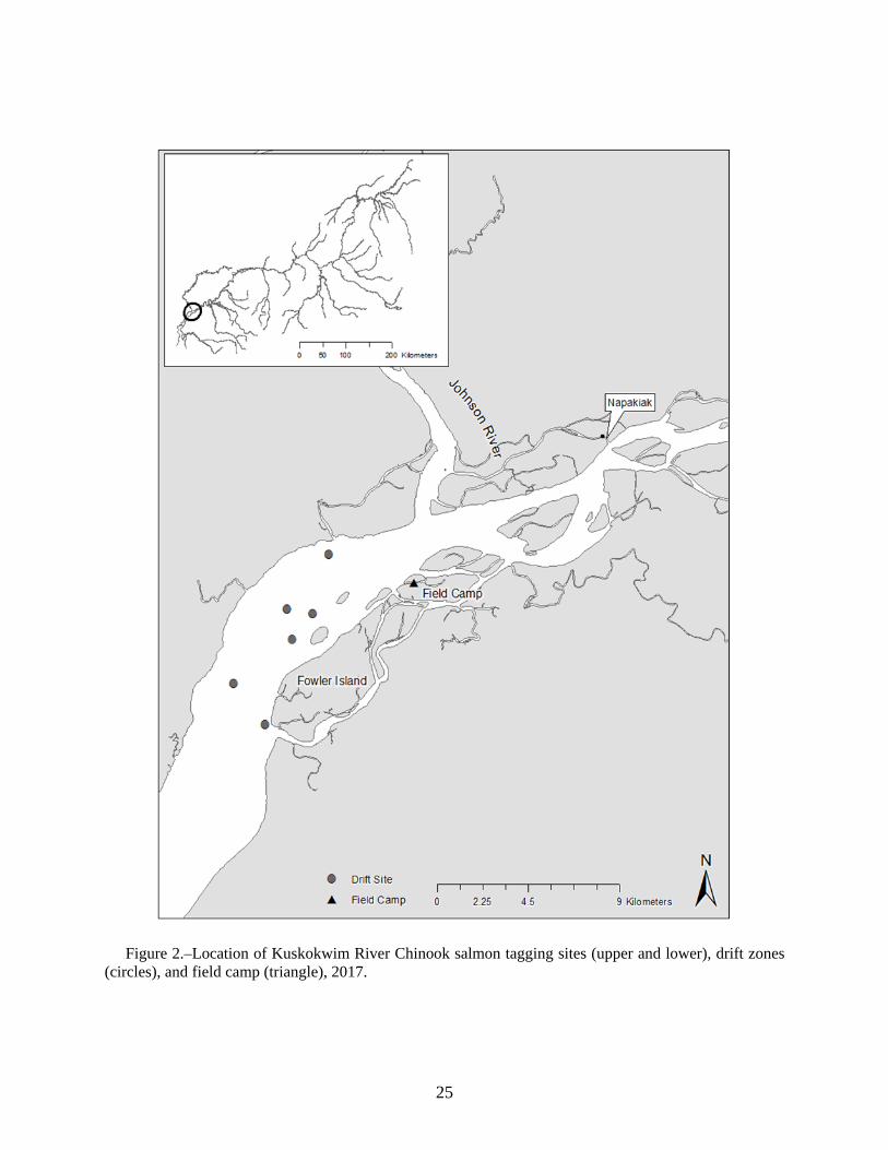
Initial capture and tagging of Chinook salmon occurred at rkm 67, near the confluence of the Johnson and Kuskokwim rivers (Figure 2). This area was chosen because it is downriver from all but 1 Chinook salmon spawning tributaries (i.e., Eek River) and downriver from where approximately 90% of subsistence harvest occurs (Shelden et al. 2016). The river channel near the tagging area was 3.7 km wide and tagging occurred along a section of the mainstem that was approximately 7 km long. Within the tagging area, 6 previously established drift zones were used to capture and tag adult Chinook salmon (Figure 2; Smith and Liller 2017b). Drift zone depths ranged 6.1–9.1 m at most sand bar locations, and 9.1–12.2 m at most bank locations. Maximum river depth was 25 m near the vicinity of the tag site.
Recapture of tagged Chinook salmon occurred at 8 weirs located on spawning tributaries within the lower, middle, and upper portions of the Kuskokwim River drainage (Figure 1). Weirs located on the Kwethluk (rkm 216) and Tuluksak (rkm 248) rivers indexed Chinook salmon spawning tributaries in the lower portion of the Kuskokwim River. Middle Kuskokwim River tributaries were indexed at weirs installed on the Salmon (Aniak drainage; rkm 404), George (rkm 453), Tatlawiksuk (rkm 568), and Kogrukluk (Holitna drainage; rkm 710) rivers. Weirs on the Takotna River (rkm 835) and Salmon River (Pitka Fork drainage; rkm 880) indexed Chinook salmon migrating to the headwaters tributaries upriver from McGrath.
A total of 12 stationary telemetry towers were used to monitor movement and determine the final fate of radiotagged Chinook salmon (Figure 1). A single telemetry station located at rkm 112 (hereafter referred to as T01) was used to identify radiotagged fish that successfully migrated upriver from the tagging location. A distance of 44 rkm separated the tagging location and T01 to allow radiotagged fish adequate time to recover from capture and tag stress. An additional 4 telemetry stations were located along the mainstem Kuskokwim River from the bifurcation of the mainstem Kuskokwim River and Kuskokuak Slough (rkm 124) to McGrath (rkm 753). A telemetry station was also located at 7 of the 8 weir recovery sites. A telemetry station was not installed at the Takotna River weir because low escapement was expected at this location.
4
MARK–RECAPTURE ABUNDANCE ESTIMATION A Petersen closed population 2-sample mark–recapture study design (Chapman 1951; Seber 1982) was used to estimate the total inriver abundance of Chinook salmon upstream of rkm 67.
First Event Sampling Fish capture operations were designed to ensure crew safety and focus fishing effort on the most active periods of Chinook salmon upriver migration. A tagging crew consisting of 3 people was utilized during daytime operations. All night tides and periods of inclement weather utilized a 4-person tagging crew in an effort to bolster safety. Sampling was conducted 7 days per week throughout the entire Chinook salmon run (May 24–July 21). The tagging crew fished for approximately 8 hours each day and effort distributed among the twice daily incoming tides started just after slack tide. Tide schedule predictions were based on a 1-hour earlier adjustment from the Bethel District in the Western Alaska edition of the Alaska Tide Book. At the start of each tide, effort was distributed evenly among drift zones (Figure 2) until it was determined where fish capture was most successful. Increased sampling effort was allocated to more productive zones throughout the remainder of the shift.
Drift gillnets were used to capture medium to large size adult Chinook salmon. Gillnets had a stretched mesh size of 7.5 in (19.1 cm) and were 45 meshes deep (8.6 m). Gillnets were constructed of multi-fiber monofilament (MT83 twine and shade 66 Green) with a K/D knot type. Size 11 closed cell foam floats were used with a 7/16″ cork line. The lead line was size 95. The mesh was hung at a 2:1 ratio for a finished length of 25 fathoms (45.7 m).
Strict handling, tagging, and release methods were used to minimize fish stress. When it was suspected that a fish was captured in a drift gillnet, the net was retrieved to the boat. Captured Chinook salmon were immediately removed from the net, placed in a tote containing fresh river water, and immobilized in a soft mesh cradle. A physical examination was performed on all captured Chinook salmon. The examination ranked fish on a scale of 1–4, with 1 being good condition with no visible injuries, 2 having minor injuries, 3 having major injuries, and 4 being deceased. Only fish that receive a rank of 1 or 2 were tagged. Chinook salmon were released immediately after tagging.
All Chinook salmon greater than 450 mideye to tail fork (METF) length that passed the physical examination were given a primary mark consisting of a uniquely numbered spaghetti tag (Model FT-4; Floy Tag and Manufacturing, Inc.1), and a subset of 157 Chinook salmon also received an esophageal radio tag (Advanced Telemetry Systems). Spaghetti tags were attached approximately 1 cm below and 2–3 fin rays anterior to the posterior insertion of the dorsal fin following standard methods. Radio tags were deployed in proportion to run strength based on a schedule developed from historic run timings observed at the Bethel test fishery (BTF) located 39 rkm upriver from the tag site. Inseason run timing information from the BTF was used to modify the deployment schedule to mimic actual run timing observed. Each radio tag was distinguishable by a unique frequency and encoded pulse pattern. Two different sized radio tags were used to ensure that tag weight did not exceed 2% of the fish’s body weight (Cooke et al. 2012). A model F1840B tag (20 grams total weight) was used for fish with METF length between 450 mm and 550 mm. A larger model F1845B tag (24 grams total weight) was used for
1 Product names used in this report are included for scientific completeness but do not constitute a product endorsement.
5
fish with a METF length greater than 550 mm. Insertion of radio tags followed standard methods (e.g., Stuby 2007).
Tag information and biological data was recorded for all captured Chinook salmon at the time of tagging. Data included the spaghetti tag number, radio tag frequency and code, METF length (mm), sex, and fish condition. Sex was determined by visually examining secondary sexual characteristics. All non-target species captured were recorded and released.
The number of spaghetti tagged Chinook salmon that continued upriver past the tag site was estimated using information collected from radiotagged fish. The number of radiotagged fish that continued upriver past the tag site (nrup) was equal to the sum of the fish harvested between the tag site and T01 and those fish that moved and remained upriver past T01. That subset (nrup) of radiotagged fish out of the total number of radiotagged fish released at the tag site (nr) formed the estimated proportion of tagged fish that were available for recapture (pup = nrup /nr). Then, the number of spaghetti tagged fish that successfully migrated upriver from the tagging site ( 'M ) out of the total number of fish that received a spaghetti tag (M) was estimated as M·pup. All fish harvested downriver from the tag site and those that did not resume migration past the tag site were culled from the experiment.
Telemetry Tracking The subset of spaghetti tagged Chinook salmon that also received a radio tag were tracked along the mainstem Kuskokwim River using a network of 5 stationary tracking towers (Figure 1). Each stationary tower was equipped with an ATS model 4500 receiver that had an integrated data logger. The receiver, 2 deep-cycle 12V batteries, and associated components were securely housed in a lockable weather resistant steel box. Two 4-element Yagi antennas were mounted on a mast elevated 2–10 m above the ground. The tower was powered by a 95W solar panel. The receiver was programmed to receive from both antennas simultaneously and scan through the list of tag frequencies at 6 s intervals. When a signal of sufficient strength was encountered, the receiver paused for up to 12 s on each antenna to decode and record tag information. The relatively short cycle period minimized the chance of a radiotagged fish passing the receiver site without being detected.
A series of 15 aerial telemetry tracking flights were performed between June 13 and August 21 to assist with monitoring upriver movement and determine a final fate for radiotagged fish (Table 1). Inseason tracking flights, which occurred June 13 to August 16, were conducted by U.S. Fish and Wildlife Service (USFWS) as part of a separate study that was designed to characterize Chinook salmon migration characteristics within the Kwethluk, Kasigluk, Kisaralik, and Tuluksak rivers. USFWS provided ADF&G with all tracking data which were used to subsidize postseason tracking efforts conducted by ADF&G from August 19 to August 21. Tracking surveys were conducted with a fixed wing aircraft, pilot, and surveyor(s) who operated a R4500 data logger(s). Scan time for each frequency was 2 seconds. A single H-antenna was mounted on each wing strut, and the surveys conducted August 19–21 also utilized a C-type antenna attached to the bottom of the aircraft. The H-type antenna provided directional detection of fish to the left or right side of plane. The C-type antenna was used to increase detection of tagged fish directly below the plane. Surveys were flown at approximately 120 km/h at an altitude between 100 m and 300 m above the center of the river. Once a radio tag was detected, the surveyor prompted the data logger to record georeferenced tag information.
6
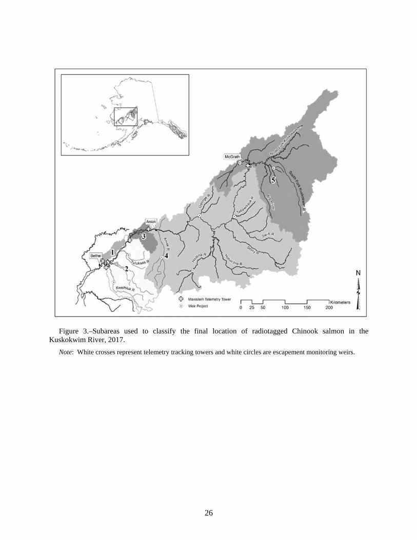
The combination of stationary and aerial telemetry tracking methods were used to monitor movement, determine the final fate of radiotagged Chinook salmon, and test mark–recapture assumptions. The Kuskokwim River drainage was stratified into 5 subareas upriver from rkm 112 using the network of 5 towers along the mainstem (Table 2; Figure 3). A process of elimination approach was used to assign fish to a subarea and determine a final fate (Liller et al. 2011). Chinook salmon were assumed to be in a tributary if stationary tower records confirmed their presence in a subarea and they were not detected in the mainstem during the aerial tracking survey. A single tracking tower was located at 7 of the recapture weirs to determine the number of radiotagged Chinook salmon that passed upriver. Aerial survey flights were flown upriver from each weir to confirm the passage of radiotagged fish through the recapture weirs, in the unlikely event that a tagged fish passed the tower undetected.
Harvest Mortality Harvest mortality of tagged fish was evaluated using a volunteer tag lottery. The lottery was advertised using mailers sent to rural businesses and tags were clearly labeled with contact information. Fishermen were encouraged to report tags caught in the subsistence fishery by advertising 4 individual monthly prizes of $200 awarded to a randomly selected participant who reported tag information. A grand prize drawing was held at the end of the study and awarded a $500 prize to 1 participant selected at random from all monthly participants. Participants reported the date and location of harvested fish along with tag color, tag number, and presence or absence of a radio tag.
Radiotelemetry methods were also used to determine if a radiotagged fish may have been harvested but was not reported through the lottery system. A radiotagged fish was assumed to have been harvested if it was identified in the same location within 1 km of a village or active fish camp for 3 or more aerial tracking flights.
Second Event Sampling Methods Recapture sampling occurred at 8 tributary escapement monitoring weirs located upstream of the tagging location. The planned operational dates for each weir have been shown to encompass the entire Chinook salmon escapement at each location (Table 3; Head and Liller 2017; Webber et al. 2016a and 2016b). Recapture samples collected at each of the 8 weir locations (Ci) consisted of all Chinook salmon observed passing upstream of weir (i) (i = 1,…, 8) during operable periods. The total recapture sample (C) was ∑(Ci). Only fish directly counted at the weir were included in the sample; estimates of missed passage were not used.
All Chinook salmon were visually inspected for spaghetti tags as they passed weir locations. External tag identification and reporting was accomplished using 2 methods. ADF&G staff physically recaptured tagged fish as they passed weirs located on the George, Tatlawiksuk, Kogrukluk, and Salmon (Pitka drainage) rivers (Head and Liller 2017). Staff from the Native Village of Napaimute and MTNT, Ltd. physically recaptured tagged fish at weirs on the Salmon (Aniak drainage) and Takotna rivers, respectively, following ADF&G methods. When a tagged fish was recaptured at the weir, tag number, presence of a radio tag, sex, and condition of the fish were recorded. Weirs operated by USFWS on the Kwethluk and Tuluksak rivers utilized video technology to enumerate passing Chinook salmon (Webber et al. 2016a and 2016b). Presence of a tag and tag color was visible to observers who reviewed recorded footage of fish passing the weir, but tag numbers were only recorded for a small subset fish recaptured during scheduled age, sex, and length sampling periods. Video data was reviewed both inseason and postseason
7
and compared to data from the nearby telemetry tower to confirm that all tagged fish were identified.
The number of tag recaptures was adjusted to account for incomplete reporting by weir crews. The number of radiotagged Chinook salmon that passed upriver of each weir was known from telemetry tower and air survey records. However, it was recognized that some portion of the fish that only received an external spaghetti tag may have passed upriver through the weir without being observed. Radiotelemetry data was used to estimate the probability that a tagged fish was observed as it passed through the weir during operational periods. Recapture sites were grouped based on recapture performance (p; p = 1 and 2). The number of radiotagged fish detected by the telemetry towers located at the weir sites (ntp) and the total number of radio tags documented by weir staff (nsp) was used to estimate the detection probability (psp=nsp/ntp) for each group. Then the detection probability and the number of spaghetti tag only recaptures (rp) was used to estimate total number of non-radiotagged fish that passed the weirs (Rp) as rp/psp. The expected total number of recaptures (R') was then estimated as ∑ (Rp +ntp).
Groups were defined as follows for the purpose of estimating detection probability. Weirs on the Kwethluk, Tuluksak, Salmon (Aniak), George, Tatlawiksuk, and Takotna rivers were grouped because each of these projects had 100% observation of fish that had a radio tag. The Kogrukluk and Salmon (Pitka Fork) River weirs were grouped because these locations experienced periods where tagged fish migrated upriver of the weir undetected and used the same methods to observe fish.
Data Analysis Chapman’s modification of the Petersen estimator (Chapman 1951; Seber 1982) was used to estimate total abundance of Chinook salmon upstream of rkm 67:
N�= (M'+1)(C+1)R'+1
-1 . (1)
Variance of the mark–recapture estimate was estimated by a parametric bootstrap simulation with 1,000 replicates (Efron 1982). Each uncertain parameter, M′, psp, and R′ associated with the tagging and recapturing processes was modeled and denoted in subsequent equations with an asterisk (*). With each bootstrap replicate, denoted with subscript (b), a probable value for each parameter was drawn from an assumed distribution and a bootstrap estimate of simulated abundance was calculated using Equation 1.
The number of spaghetti-tagged fish that moved upstream of the tag site was assumed to have a binomial distribution (BN), and was modeled as M*(b)~BN (M,pup).
Estimating the number of recaptures was accomplished by monitoring a subset of spaghetti tagged fish fitted with radio tags. The estimation process relied on 3 steps. Because the estimated number of fish that only had spaghetti tags at each weir was predicated on the detection probability of fish that also had radio tags, the detection probability of radio tags at each weir group (p*(b)sp) was modeled as a binomial variable (p*(b)sp~BN(ntp,psp)/ntp). The second step modeled radio tag movement variability among recapture locations by separating the proportion of spaghetti tagged fish with a radio tag, pi, into 9 classes (i) (i = 0,…, 8; Table 4). The number of radio tags recovered at each weir site (ntp) was assumed to have a multinomial distribution
8
and was modeled as R*(b)i~multi(ntppi). Lastly, the results from the first 2 steps were used to model the total number of spaghetti tagged fish that were recovered as R*(b)=∑R*(b)i +∑ rp/p*(b)sp.
The average bootstrap estimate of simulated abundance (N*(b)) calculated as (∑N*(b) )/1,000 were used to approximate variance of the mark–recapture estimate, using the following equation:
v(N�)=∑ (N*(b)-N*(b))
2(b)
B-1 . (2)
The 95% confidence interval was determined from the 2.5 and 97.5 percentiles of the bootstrap distribution. The bounds of the 95% confidence interval relative to the abundance estimate were evaluated using the following equation and reported as a percentage:
�1.96√v�N
� 100 . (3)
Data modeling and hypothesis testing were used to determine whether this study met the critical assumptions of the Petersen estimator (Chapman 1951; Seber 1982). The requirement for a closed population was addressed by conducting tag and recapture operations throughout most of the Chinook salmon run and culling fish that did not continue upriver after being tagged. Because harvest occurs throughout the mark–recapture study area, tagged and untagged fish harvest rates were assumed to be the same. The assumption that tagged fish behave the same as untagged fish could not be formally evaluated, but there was an attempt to minimize behavioral effects by limiting holding time of captured fish and tagging only healthy fish. The requirement that fish retain their tag and are recognized during the second sample event was addressed by estimating the proportion of fish that were observed at each weir and adjusting the number of recaptures with this proportion. The assumption that all fish had an equal probability of capture in the first or second sample was evaluated using radiotagged fish and by following recommendations of Seber (1982; Appendix A1). Although Seber (1982) recommended using a chi-square statistic, this test was not appropriate due to small sizes. Therefore, Fisher’s exact test was used to evaluate equal probability of capture and recapture because this test accounts for zeros and does not require non-sensical pooling to meet the sample size requirements needed to use the chi-square statistic.
Sex and length selectivity biases that may have occurred during the capture and recapture events were explored using contingency table analysis and a Kolmogorov-Smirnov test. Comparisons of the marked (M) and recaptured (R) populations for sex and length used standard chi-square and Kolmogorov-Smirnov tests, respectively. However, tests involving fish examined during the second event (C) were modified to account for the fact that sex and length composition of fish examined in the second event was estimated, and the number of samples collected at each site was not proportional to abundance. The sex composition of the recapture sampling event (S) was estimated by weighting the sex ratio (s) observed at each weir (i) (i = 1,…, 8) by the escapement at that weir (Ci), so that S=∑Ci�si. A chi-square test of independence was used to test the hypothesis of no difference in the sex composition between the first and second sampling event. In order to evaluate length bias, an empirical cumulative distribution function for the second sampling event was modeled. The count (l) of samples collected at each discrete length (m) (m = 365…, 1,050) was expanded by the total escapement (Ci) at each recapture weir, and the expanded count of lengths was summed across all weir locations as:
9
Fm=∑� lmi∑ lmi
� Ci� .
(4)
The estimated count of fish by length in the recapture sample was converted to a cumulative distribution and compared to cumulative length distribution of the marked sample using a Kolmogorov-Smirnov goodness-of-fit test (Appendix A2). All statistical tests were considered significant at α = 0.05.
RUN TIMING Run timing past the tag site was evaluated for all radiotagged fish returning to Subareas 2, 4, and 5 (Figure 3) using all available telemetry (tower and aerial) and recapture (weir and tributary harvested tag returns) information. Subareas 1 and 3 were not included because no Chinook salmon tributaries drain into those sections. Tag dates recorded at the lower river site were summarized using the median, central 50%, and central 80% of fish returning to each subarea. Date summaries were portrayed graphically for comparison and trend identification.
MIGRATION RATE Radiotelemetry data was used to determine the total time it took for each radiotagged Chinook salmon to travel between successive locations (i) along the mainstem Kuskokwim River. Elapsed time was estimated between the tag site (i = 0) and tower T01 and then sequentially between each successive pair of tower locations (i = 1,…, 5) moving upriver. The date, hour, and minute (t) at which each fish was released at the tag site was known. The date, hour, and minute that each fish passed tower (i) was approximated using the first detection by the upriver antenna. The estimated total elapsed time (T′) between locations was estimated as ti-t(i-1) and reported in days. The distance (d) between each location (i) was determined using ArcGIS® software. A migration rate was determined for each fish as Ti′/di. Radiotagged fish assigned to Subareas 2, 4, and 5 were pooled by subarea and a median migration rate and interquartile range (IQR) was calculated.
RESULTS The estimated abundance of Chinook salmon upstream of rkm 67 was 125,339 fish (95% CI: 95,954–149,842; Table 5). The abundance estimate includes all fish that were harvested or escaped upriver from the tag site at rkm 67. The bounds of the 95% confidence interval were ±22% of the estimated abundance, which met the predetermined objective criteria of ±25% (Robson and Regier 1964).
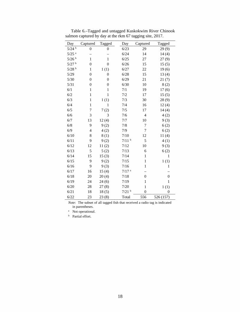
A total of 556 Chinook salmon were captured at rkm 67. Of the captured fish, 526 (95%) Chinook salmon were spaghetti tagged and a subset of 157 fish also received a radio tag (Table 6). Chinook salmon were initially captured on the third day of tagging operations. Catches steadily increased and peaked at 30 Chinook salmon on July 3. A maximum of 1 fish daily was caught during the last 8 days of operations. No fish were captured on the final day of operations (July 21).
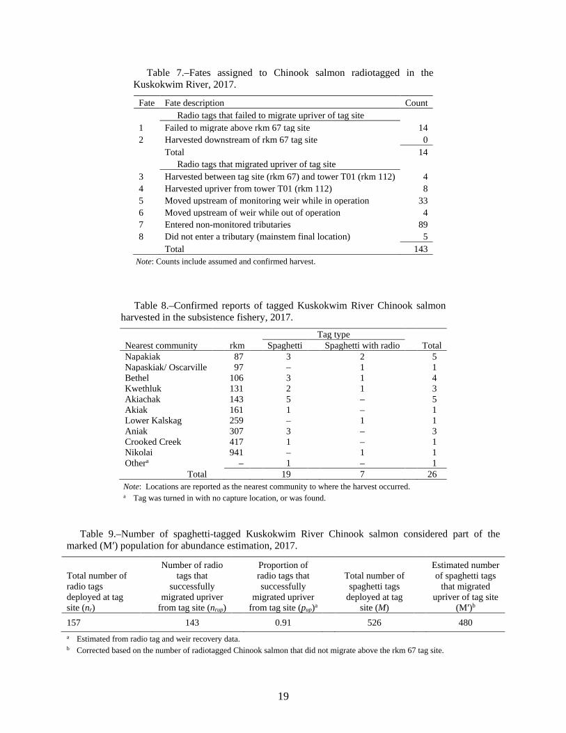
Final fate was determined for all 157 radiotagged Chinook salmon (Table 7). A total of 14 (9%) radiotagged fish failed to migrate and remained upriver from the tag site. Of those, 11 did not resume upriver migration, and 3 continued upriver past T01, but later moved downriver out of the study area. A total of 143 (91%) radiotagged fish migrated upriver of T01. Of those, 139 (97%) radiotagged Chinook salmon migrated and remained upriver from T01, whereas 4 (3%)
10
fish were harvested between the tag site and T01. Of the 139 fish that passed T01, a total of 126 (90%) radiotagged fish were in a spawning tributary, 5 (4%) were in the mainstem Kuskokwim River, and 8 (6%) were harvested in the subsistence fishery upriver from T01.
A total of 26 tagged Chinook salmon were confirmed reported harvests in the local subsistence fishery (Table 8). Of those, 19 (73%) were fish tagged with only a spaghetti tag and 7 (27%) were also tagged with a radio tag. Most harvest (73%) occurred in the lower portion of the Kuskokwim River (i.e., lower 200 rkm), and 38% of harvest occurred between Napakiak (rkm 87) and Bethel (rkm 106).
The number of spaghetti-tagged Chinook salmon that continued upriver after being released at rkm 67 was estimated using radiotelemetry and harvest reports. The proportion of spaghetti tagged fish that migrated and remained upriver from T01 (pup) was estimated to be 0.91 (Table 9). Therefore, the total number of spaghetti-tagged fish was reduced by 9% to account for fish that did not continue upriver past the tag site. The total estimated marked population after correction (M′) was 480 spaghetti tags (Table 9).
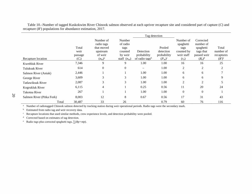
Total observed escapement (C) from all 8 weirs was 30,487 Chinook salmon (Table 10). A total of 86 tagged Chinook salmon were observed by weir crews during operational periods, of which 60 had only a spaghetti tag and 26 had both a spaghetti and radio tag. The probability that a spaghetti tagged fish was observed passing through the weirs varied. Factors that contributed to this included high water events and the volume of fish passing at the time of observation (Table 10). The lowest detection probability (0.25) occurred at the Kogrukluk River weir. The Salmon River (Pitka Fork) weir had a detection probability of 0.67. Spaghetti tags were only estimated for the Kogrukluk River and Salmon River (Pitka Fork) using a pooled detection probability. A pooled estimate of tag detection was used because the Kogrukluk River weir had small sample sizes of radio tags available to inform detection probability and both weirs suffered from the same issue of not detecting tagged fish migrating upriver of the weir due to unfavorable water conditions. All other weirs had 100% detection of Chinook salmon fitted with a radio tag. Total estimated tag recoveries (R′) were 116 tags after adjusting for tagged fish that passed weirs undetected (Table 10).
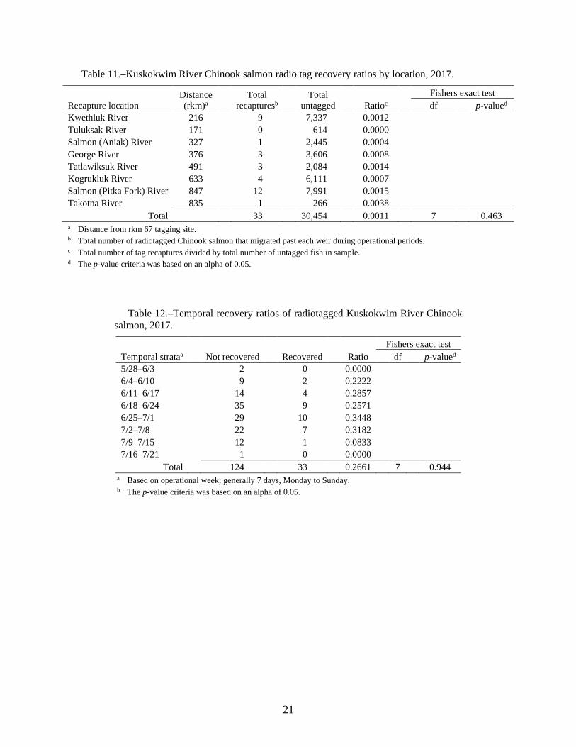
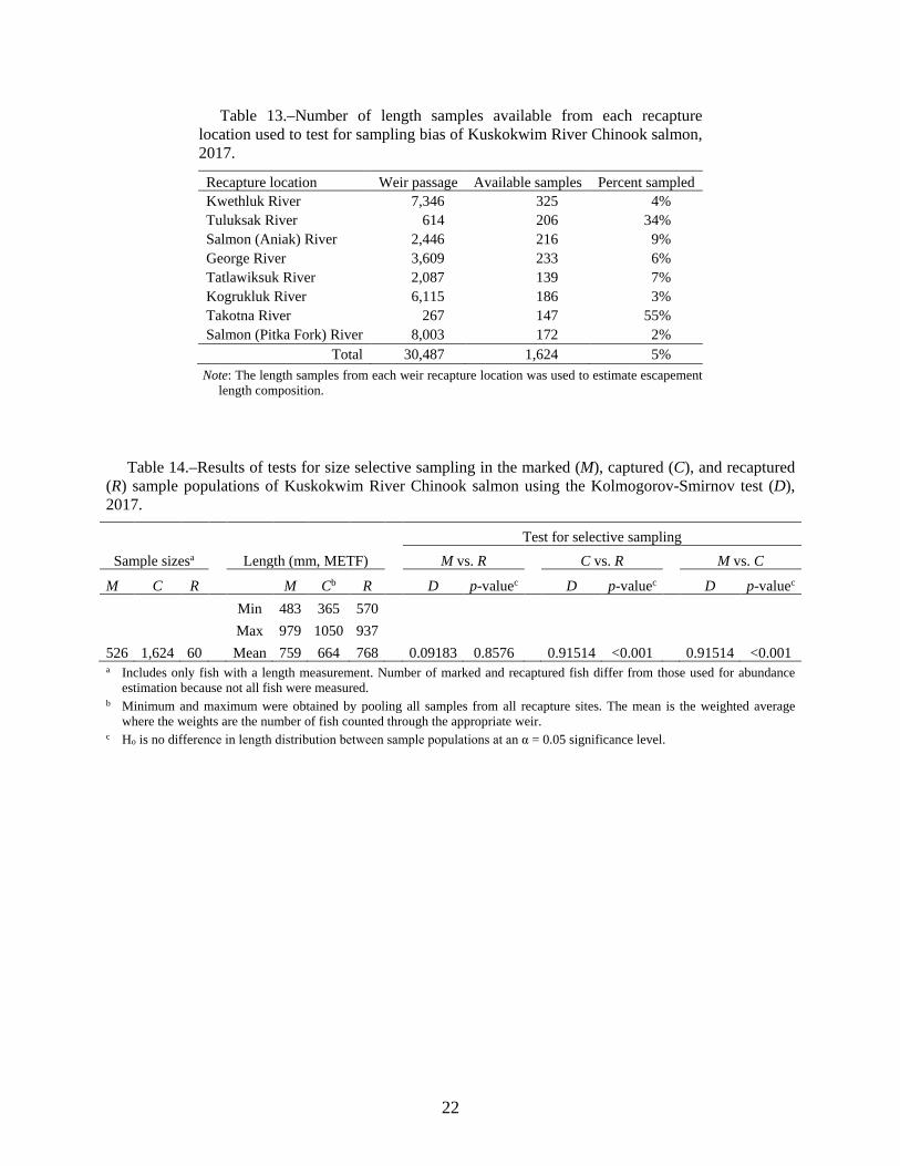
Conditions for an unbiased estimate of abundance were achieved. The ratio of marked and unmarked radiotagged Chinook salmon at each weir was not significantly different, which provided support for the assumption of equal probability of capture (Table 11; p = 0.463). Additionally, temporal radio tag deployment and recapture ratios were not significantly different (Table 12; p = 0.944), which indicated the probability of a tagged fish being recaptured did not vary over the course of the study. Large sample sizes were available to detect length biases (Table 13). There was evidence that the first sampling event disproportionately selected larger fish; however, there was no length selectivity during the second event (Table 14; Figure 4). As a result, population composition parameters for length data are best represented by data collected from the weirs. Sex assignment at the tagging location was unreliable based on postseason validation. Therefore, tests for sex selective sampling are not presented.
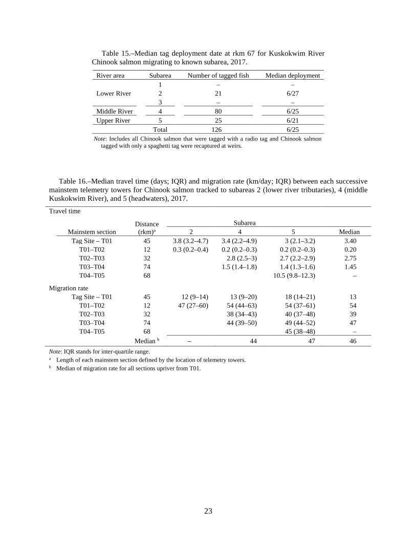
RUN TIMING Chinook salmon substocks overlapped considerably as they passed upriver of the tag site, but general run timing patterns were elucidated (Tables 15; Figure 5). The median tag date for fish returning to upriver tributaries was June 21, which was 4 days earlier compared to fish returning to middle river tributaries and 6 days earlier than fish returning to lower river tributaries. Fish
11
returning to middle and lower river tributaries displayed similar run timing with median catch dates of June 25 and June 27 respectively (Table 14).
MIGRATION RATE All substocks displayed similar migration rates through the sequential mainstem reaches (Table 16). It took the various substocks a median of 3.4 days to travel the 45 rkm separating the tag site and T01 at a median rate of 13 km per day (range: 12–18). Upriver migration rate increased after T01 and remained relatively consistent at a median of 46 km per day (range: 38–54) through all subsequent sections.
DISCUSSION MARK–RECAPTURE There was no evidence that tagging efforts missed a substantial temporal component of the Chinook salmon run in 2017. Less than 1% of the Chinook salmon run migrated through the lower Kuskokwim River prior to the start of tagging operations, based on information from the upriver Bethel test fishery (BTF; rkm 106; AYKDBMS2). The BTF utilized drift gillnets to assess daily inseason run strength and timing of Kuskokwim River salmon migrating upriver past Bethel (Lipka and Elison 2016). Tagging operations continued as planned and on schedule throughout the run. Low catches during the last week of operations provided a reasonable assurance that the end of the run was well represented. Only 3.8% of the Chinook salmon run passed the BTF location after tagging operations ceased downriver.
Overall detection of tagged fish at recovery weirs was high. Of the 8 recovery locations, 6 had perfect visual detection of fish that received both spaghetti and radio tags. The Salmon River (Pitka Fork) weir had overall good detection and only missed a few fish in the early part of the season when a large pulse of fish had to be counted through the weir using nonstandard methods. Chinook salmon were milling below the weir during a period of low clear water conditions. Several sections of weir were removed to facilitate passage of these milling fish. Counts during this period were accurate, but tag detection was reduced during this time. The Kogrukluk River weir encountered several high-water events throughout the course of the Chinook salmon run that inhibited ideal tag detection conditions. Although the mechanism that resulted in reduced tag detection was different between the Salmon River (Pitka Fork) and Kogrukluk River weirs, the result was the same – undocumented tags moved upstream of the weir. As such, a pooled estimate of tag detection was used to estimate the number of missed spaghetti tags migrating above the Salmon River (Pitka Fork) and Kogrukluk River weirs similar to Smith and Liller (2017a-b). An abundance estimate based on un-pooled estimates of tag recaptures was generated to investigate the effect of pooling detection probability for Salmon River (Pitka Fork) and Kogrukluk River weirs. The resulting point estimate fell within the 95% confidence interval based on pooled detection as presented in this report. Therefore, the interpretation of run size would be the same between the 2 methods.
Similar to mark–recapture studies conducted from 2014 to 2016, it was unknown why a portion of radiotagged fish (7 in 2017) had a final location in the mainstem Kuskokwim River upriver from T01; however, it is unlikely that this uncertainty substantially influenced the abundance 2 AYKDBMS [Arctic-Yukon-Kuskokwim Database Management System] Home Page. http://sf.adfg.state.ak.us/CommFishR3/WebSite/AYKDBMSWebsite/Default.aspx.
estimate for 2017. There are no known Chinook salmon spawning aggregates in mainstem Kuskokwim River. Therefore, tagged fish located in the mainstem probably represent a combination of tag loss, unreported harvested fish, and fish that expired during upriver migration. Efforts to curb unreported harvests have been made in recent years by labelling fish as likely harvests when repeatedly recorded by aerial tracking flights within 1 km of a village. Also, unreported harvest would not affect the abundance estimate if tagged and untagged fish were harvested in similar proportions, which was considered a reasonable assumption. In addition to harvest mortality, some degree of natural mortality was expected as fish travel upriver towards spawning grounds (e.g., Cooke et al. 2006), and it was assumed that tagged and untagged fish would succumb to natural mortality at similar rates. However, it is plausible that the addition of tagging and handling stress may have resulted in higher enroute mortality for tagged fish. As such, it is possible that a few of these 7 fish were bound for monitored tributaries, and if they had not died, may have been recaptures. An attempt to account for this type of uncertainty was included in variance estimation by modeling recaptures and simulating abundance.
The reduction in 2017 telemetry infrastructure decreased the spatial resolution of substock specific run timing and migration speed. Available run timing and migration data were adequate to draw broad conclusions. Overall, general run timing patterns observed in 2017 were consistent with 2015 and 2016 observations. Tributaries upriver from McGrath had earlier migration timing compared to fish returning to spawn in less distant tributaries, and tagged fish tended to travel a similar and nearly consistent rate, regardless of the tributary of return.
RECOMMENDATIONS The study objective was fulfilled using a reduced initial tagging effort of 1 tagging crew. The single fishing crew captured approximately half the number of fish that 2 fishing crews caught during the 2015 season, and a third the number of fish captured during the 2016 season. Similar to the 2 crew study design of 2015 and 2016, the abundance calculated for 2017 was also within the desired level of accuracy (±25%; Smith and Liller 2017a and 2017b). Future studies that aim to only estimate abundance can continue to use this streamlined sampling approach.
Radiotagging all captured fish would increase the robustness of this study design. Using radio tags as the primary mark would allow us to determine a final fate for all tagged fish and would eliminate the need to estimate the number of marks and recaptures. Furthermore, because all radio tag recaptures can be positively verified, the second sample could be increased by using estimates of missed passage during brief periods when weirs are not operational. A single boat crew has been shown capable of capturing and tagging around 550 fish in the lower Kuskokwim River. Radiotagging all fish would increase the sample size of radio tags to 2015 and 2016 sample levels, which would allow confident estimation of migration characteristics. The cost of this change to study design would be solely in the increased cost of radio tags because the amount of personnel time to radio tag and track every fish would be negligible.
ACKNOWLEDGEMENTS Without the support and cooperation of many individuals and organizations this project would not have been possible. We thank the Pacific States Marine Fisheries Commission for providing funding for this study, and the Bering Sea Fisherman’s Association for facilitating the award (Pacific States Marine Fisheries Commission Award Number 17-91G). Division of Commercial Fisheries tagging and telemetry staff members Carlton Hautala, Michael McNulty, Morgan
13
MacConnell, RJ Lister, and Hannah Puterbaugh were an invaluable part of this project. Commercial Fisheries weir staff, especially Rob Stewart, was vital to the success of this project. USFWS biologists (Ken Harper and Aaron Webber) and technicians made it possible to incorporate the Kwethluk and Tuluksak weirs into the study design and Aaron Moses provided a vast amount of radiotelemetry tracking support. Lastly, we would like to thank all the Kuskokwim River residents that contributed to this study through their support and participation in volunteer tag recovery program. Xinxian Zhang provided biometric review for this report. Zachary Liller provided regional review and assisted in early phases of project development and oversight.
REFERENCES CITED ADF&G Chinook Salmon Research Team. 2013. Chinook salmon stock assessment and research plan, 2013.
Alaska Department of Fish and Game, Special Publication No. 13-01, Anchorage.
Bue, B. G., K. L. Schaberg, Z. W. Liller, and D. B. Molyneaux. 2012. Estimates of the historic run and escapement for the Chinook salmon stock returning to the Kuskokwim River, 1976-2011. Alaska Department of Fish and Game, Fishery Data Series No. 12-49, Anchorage.
Chapman, D. G. 1951. Some properties of the hypergeometric distribution with applications to zoological censuses. University of California Publications in Statistics 1:131–160.
Cooke, S. J., S. G. Hinch, G. T. Crossin, D. A. Patterson, K. K. English, M. C. Healey, J. M. Shrimpton, G. V. D. Kraak, and A. P. Farrell. 2006. Mechanistic basis of individual mortality in Pacific salmon during spawning migrations. Ecology 87:1575–1586
Cooke, S. J., S. G. Hinch, M. C. Lucas, and M. Lutcavage. 2012. Biotelemetry and biologging. Pages 819-860 [In]: A. V. Zale, D. L. Parrish, and T. M. Sutton, editors, Fisheries techniques third edition. American Fisheries Society, Bethesda, Maryland.
Efron, B. 1982. The jackknife, the bootstrap, and other resampling plans. Society for Industrial and Applied Mathematics. Philadelphia.
Fall, J. A., C. L. Brown, S.S. Evans, R. A. Grant, H. Ikuta, L. Hutchinson-Scarbrough, B. Jones, M. A. Marchioni, E. Mikow, J. T. Ream, L. A. Sill, and T. Lemons. 2015. Alaska subsistence and personal use salmon fisheries 2013 annual report. Alaska Department of Fish and Game, Division of Subsistence, Technical Paper No. 413, Anchorage.
Head, J. H., and Z. W. Liller. 2017. Salmon escapement monitoring in the Kuskokwim Area, 2016. Alaska Department of Fish and Game, Fishery Data Series No. 17-29, Anchorage.
Head, J. M., N. J. Smith, and Z. W. Liller. 2017. Inriver abundance of Kuskokwim River Chinook salmon, 2014. Alaska Department of Fish and Game, Fishery Data Series No. 17-23, Anchorage
Liller, Z. W., K. L. Schaberg, and J. R. Jasper. 2011. Effects of holding time in a fish wheel live box on upstream migration of Kuskokwim River Chum salmon. Alaska Department of Fish and Game, Fishery Data Series No. 11-34, Anchorage.
Liller, Z. W. 2017. 2016 Kuskokwim River Chinook salmon run reconstruction and 2017 forecast. Alaska Department of Fish and Game, Division of Commercial Fisheries, Regional Information Report 3A17-02, Anchorage.
Lipka, C., and T. Elison. 2016. Characterization of the 2012 and 2013 salmon runs in the Kuskokwim River based the test fishery at Bethel. Alaska Department of Fish and Game, Fishery Data Series No. 16-06, Anchorage.
Robson, D. S., and H. A. Regier. 1964. Sample size in Petersen mark-recapture experiments. Transactions of the American Fisheries Society 93:215-216.
Schaberg, K. L., Z. W. Liller, and D. B. Molyneaux. 2010. A mark–recapture study of Kuskokwim River coho, chum, sockeye, and Chinook salmon, 2001–2006. Alaska Department of Fish and Game, Fishery Data Series No. 10-32, Anchorage.
14
REFERENCES CITED (Continued) Schaberg, K. L., Z. W. Liller, D. B. Molyneaux, B. G. Bue, and L. Stuby. 2012. Estimates of total annual return of
Chinook salmon to the Kuskokwim River, 2002–2007. Alaska Department of Fish and Game, Fishery Data Series No. 12-36, Anchorage.
Seber, G. A. F. 1982. The estimation of animal abundance and related parameters, second edition. Edward Arnold, London.
Shelden, C. A., T. Hamazaki, M. Horne-Brine, I. Dull, and R. Frye. 2016. Subsistence salmon harvests in the Kuskokwim area, 2014. Alaska Department of Fish and Game, Fishery Data Series No. 16-49, Anchorage.
Smith, N. J., and Z. W. Liller. 2017a. Inriver abundance and migration characteristics of Kuskokwim River Chinook salmon, 2015. Alaska Department of Fish and Game, Fishery Data Series No. 17-22, Anchorage.
Smith, N. J., and Z. W. Liller. 2017b. Inriver abundance and migration characteristics of Kuskokwim River Chinook salmon, 2016. Alaska Department of Fish and Game, Fishery Data Series No. 17-47, Anchorage.
Smith, N. J., and Z. W. Liller. 2018. 2017 Kuskokwim River Chinook salmon run reconstruction and 2018 forecast. Alaska Department of Fish and Game, Division of Commercial Fisheries, Regional Information Report 3A18-02, Anchorage.
Stuby, L. 2007. Inriver abundance of Chinook salmon in the Kuskokwim River, 2002-2006. Alaska Department of Fish and Game, Fishery Data Series No. 07-93, Anchorage.
Webber, A. P., J. K. Boersma, and K. C. Harper. 2016a. Abundance and run timing of adult Pacific salmon in the Kwethluk River, Yukon Delta National Wildlife Refuge, Alaska 2015. U.S. Fish and Wildlife Service, Alaska Fisheries Data Series No. 2016-7, Soldotna.
Webber, A. P., J. K. Boersma, and K. C. Harper. 2016b. Abundance and run timing of adult Pacific salmon in the Tuluksak River, Yukon Delta National Wildlife Refuge, Alaska 2015. U.S. Fish and Wildlife Service, Alaska Fisheries Data Series No. 2016-5, Soldotna.
15
TABLES AND FIGURES
16
Table 1.–Summary of aerial telemetry tracking surveys used to locate radiotagged Chinook salmon in the Kuskokwim River, 2017.
Mainstema Date Agency Start End Tributary 6/13 USFWS Fowler Island Tuluksak Kwethluk, Kasigluk, Kisaralik, and Tuluksak rivers 6/16 USFWS Fowler Island Tuluksak Kwethluk and Kisaralik rivers 6/20 USFWS Fowler Island Tuluksak Kwethluk, Kasigluk, Kisaralik, and Tuluksak rivers 6/23 USFWS Fowler Island Tuluksak Kwethluk and Kisaralik rivers 6/27 USFWS Fowler Island Tuluksak Kwethluk, Kasigluk, Kisaralik, and Tuluksak rivers 6/30 USFWS Fowler Island Tuluksak Kwethluk and Kisaralik rivers 7/5 USFWS Fowler Island Tuluksak Kwethluk, Kasigluk, Kisaralik, and Tuluksak rivers 7/11 USFWS Fowler Island Tuluksak Kwethluk, Kasigluk, Kisaralik, and Tuluksak rivers 7/14 USFWS Fowler Island Tuluksak Kwethluk and Kisaralik rivers 7/20 USFWS Fowler Island Tuluksak Kwethluk, Kasigluk, Kisaralik, and Tuluksak rivers 8/8 USFWS Fowler Island Tuluksak Kwethluk, Kasigluk, Kisaralik, and Tuluksak rivers 8/16 USFWS Fowler Island Tuluksak Kwethluk and Kisaralik rivers
Middle Fork (Blackwater, Big River, Pitka Fork (Excluding Salmon R.), South Fork (Tonza), East Fork, North Fork, Nixon Fork
17
Table 3.–Operational periods and inoperable days at Kuskokwim Area weir projects, 2017.
Project Operational period Weir inoperable Kwethluk River weir a 3 June–10 September 12 July; 8 August Tuluksak River weir a 9 June–9 September 3, 4, 5, 6, 26 August Salmon River (Aniak) weir 28 June–2 August 28 June; 9, 30, 31 July George River weir 14 June–13 September 17 June; 21 July; 3, 11 August Kogrukluk River weir 23 June–25 August 26 July; 25 August
Tatlawiksuk River weir 15 June–13 September 16, 20 June; 11, 19, 24–27 July; 3, 4, 8, 14 August; 6, 8, 10 September
Takotna River weir 1 July–3 August 7, 8, 18, 22 July; 3 August Salmon River (Pitka Fork) weir 20 June–10 August 20 June; 22, 23 July a Weirs on the Kwethluk and Tuluksak rivers were operated by the U.S. Fish and Wildlife Service.
Table 4.–The 9 mutually exclusive classes used to separate radiotagged
Kuskokwim River Chinook salmon for variance estimation, 2017.
Class Description p0 Entered marked population but moved to non-terminal area or harvested p1 Moved upstream of Kwethluk River Weir p2 Moved upstream of Tuluksak River weir p3 Moved upstream of Salmon River (Aniak River) weir p4 Moved upstream of George River weir p5 Moved upstream of Kogrukluk River weir p6 Moved upstream of Tatlawiksuk River weir p7 Moved upriver of Salmon River (Pitka Fork) weir p8 Moved upriver of Takotna River weir
Table 5.–Kuskokwim River Chinook salmon abundance estimate worksheet, 2017.
Number marked (M′)a
Number examined
(C) Number
recovered
Adjusted recovered
(R′)b Marked fraction
Abundance estimate L 95% CI U 95% CI
480 30,487 86 116 0.38% 125,339 95,954 149,842 a Corrected based on the percentage of radiotagged Chinook salmon that successfully migrated above the rkm 67 tagging
location. b Corrected based on detection probability.
18
Table 6.–Tagged and untagged Kuskokwim River Chinook salmon captured by day at the rkm 67 tagging site, 2017.
in parentheses. a Not operational. b Partial effort.
19
Table 7.–Fates assigned to Chinook salmon radiotagged in the Kuskokwim River, 2017.
Fate Fate description Count Radio tags that failed to migrate upriver of tag site 1 Failed to migrate above rkm 67 tag site 14 2 Harvested downstream of rkm 67 tag site 0 Total 14 Radio tags that migrated upriver of tag site 3 Harvested between tag site (rkm 67) and tower T01 (rkm 112) 4 4 Harvested upriver from tower T01 (rkm 112) 8 5 Moved upstream of monitoring weir while in operation 33 6 Moved upstream of weir while out of operation 4 7 Entered non-monitored tributaries 89 8 Did not enter a tributary (mainstem final location) 5 Total 143
Note: Counts include assumed and confirmed harvest.
Table 8.–Confirmed reports of tagged Kuskokwim River Chinook salmon harvested in the subsistence fishery, 2017.
Tag type Nearest community rkm Spaghetti Spaghetti with radio Total Napakiak 87 3 2 5 Napaskiak/ Oscarville 97 – 1 1 Bethel 106 3 1 4 Kwethluk 131 2 1 3 Akiachak 143 5 – 5 Akiak 161 1 – 1 Lower Kalskag 259 – 1 1 Aniak 307 3 – 3 Crooked Creek 417 1 – 1 Nikolai 941 – 1 1 Othera – 1 – 1
Total 19 7 26 Note: Locations are reported as the nearest community to where the harvest occurred. a Tag was turned in with no capture location, or was found.
Table 9.–Number of spaghetti-tagged Kuskokwim River Chinook salmon considered part of the marked (M′) population for abundance estimation, 2017.
Total number of radio tags deployed at tag site (nr)
Number of radio tags that
successfully migrated upriver
from tag site (nrup)
Proportion of radio tags that successfully
migrated upriver from tag site (pup)a
Total number of spaghetti tags
deployed at tag site (M)
Estimated number of spaghetti tags
that migrated upriver of tag site
(M′)b 157 143 0.91 526 480 a Estimated from radio tag and weir recovery data. b Corrected based on the number of radiotagged Chinook salmon that did not migrate above the rkm 67 tag site.
20
Table 10.–Number of tagged Kuskokwim River Chinook salmon observed at each upriver recapture site and considered part of capture (C) and recapture (R') populations for abundance estimation, 2017.
Total 30,487 33 26 0.79 60 76 116 a Number of radiotagged Chinook salmon detected by tracking station during weir operational periods. Radio tags were the secondary mark. b Estimated from radio tag and weir recovery data. c Recapture locations that used similar methods, crew experience levels, and detection probability were pooled. d Corrected based on estimates of tag detection. e Radio tags plus corrected spaghetti tags, ∑(Rp+ntp).
21
Table 11.–Kuskokwim River Chinook salmon radio tag recovery ratios by location, 2017.
Recapture location Distance (rkm)a
Total recapturesb
Total untagged
Ratioc
Fishers exact test df p-valued
Kwethluk River 216 9 7,337 0.0012
Tuluksak River 171 0 614 0.0000
Salmon (Aniak) River 327 1 2,445 0.0004
George River 376 3 3,606 0.0008
Tatlawiksuk River 491 3 2,084 0.0014
Kogrukluk River 633 4 6,111 0.0007
Salmon (Pitka Fork) River 847 12 7,991 0.0015
Takotna River 835 1 266 0.0038 Total 33 30,454 0.0011 7 0.463
a Distance from rkm 67 tagging site. b Total number of radiotagged Chinook salmon that migrated past each weir during operational periods. c Total number of tag recaptures divided by total number of untagged fish in sample. d The p-value criteria was based on an alpha of 0.05.
Table 12.–Temporal recovery ratios of radiotagged Kuskokwim River Chinook
salmon, 2017.
Temporal strataa
Not recovered
Recovered
Ratio Fishers exact test
df p-valued 5/28–6/3 2 0 0.0000
6/4–6/10 9 2 0.2222
6/11–6/17 14 4 0.2857
6/18–6/24 35 9 0.2571
6/25–7/1 29 10 0.3448
7/2–7/8 22 7 0.3182
7/9–7/15 12 1 0.0833
7/16–7/21 1 0 0.0000 Total 124 33 0.2661 7 0.944
a Based on operational week; generally 7 days, Monday to Sunday. b The p-value criteria was based on an alpha of 0.05.
22
Table 13.–Number of length samples available from each recapture location used to test for sampling bias of Kuskokwim River Chinook salmon, 2017.
Recapture location Weir passage Available samples Percent sampled Kwethluk River 7,346 325 4% Tuluksak River 614 206 34% Salmon (Aniak) River 2,446 216 9% George River 3,609 233 6% Tatlawiksuk River 2,087 139 7% Kogrukluk River 6,115 186 3% Takotna River 267 147 55% Salmon (Pitka Fork) River 8,003 172 2%
Total 30,487 1,624 5% Note: The length samples from each weir recapture location was used to estimate escapement
length composition.
Table 14.–Results of tests for size selective sampling in the marked (M), captured (C), and recaptured
(R) sample populations of Kuskokwim River Chinook salmon using the Kolmogorov-Smirnov test (D), 2017.
Test for selective sampling Sample sizesa Length (mm, METF) M vs. R C vs. R M vs. C
M C R M Cb R D p-valuec D p-valuec D p-valuec
Min 483 365 570 Max 979 1050 937 526 1,624 60 Mean 759 664 768 0.09183 0.8576 0.91514 <0.001 0.91514 <0.001 a Includes only fish with a length measurement. Number of marked and recaptured fish differ from those used for abundance
estimation because not all fish were measured. b Minimum and maximum were obtained by pooling all samples from all recapture sites. The mean is the weighted average
where the weights are the number of fish counted through the appropriate weir. c Ho is no difference in length distribution between sample populations at an α = 0.05 significance level.
23
Table 15.–Median tag deployment date at rkm 67 for Kuskokwim River Chinook salmon migrating to known subarea, 2017.
River area Subarea Number of tagged fish Median deployment 1 – – Lower River 2 21 6/27 3 – – Middle River 4 80 6/25 Upper River 5 25 6/21 Total 126 6/25
Note: Includes all Chinook salmon that were tagged with a radio tag and Chinook salmon tagged with only a spaghetti tag were recaptured at weirs.
Table 16.–Median travel time (days; IQR) and migration rate (km/day; IQR) between each successive
mainstem telemetry towers for Chinook salmon tracked to subareas 2 (lower river tributaries), 4 (middle Kuskokwim River), and 5 (headwaters), 2017.
Tag Site – T01 45 12 (9–14) 13 (9–20) 18 (14–21) 13 T01–T02 12 47 (27–60) 54 (44–63) 54 (37–61) 54 T02–T03 32 38 (34–43) 40 (37–48) 39 T03–T04 74 44 (39–50) 49 (44–52) 47 T04–T05 68 45 (38–48) – Median b – 44 47 46 Note: IQR stands for inter-quartile range. a Length of each mainstem section defined by the location of telemetry towers. b Median of migration rate for all sections upriver from T01.
24
Figure 1.–Location of the tagging site, telemetry towers (white crosses), and escapement monitoring
weirs (black dots) used to tag, track, and recapture Kuskokwim River Chinook salmon, 2017.
25
Figure 2.–Location of Kuskokwim River Chinook salmon tagging sites (upper and lower), drift zones
(circles), and field camp (triangle), 2017.
26
Figure 3.–Subareas used to classify the final location of radiotagged Chinook salmon in the
Kuskokwim River, 2017. Note: White crosses represent telemetry tracking towers and white circles are escapement monitoring weirs.
27
Figure 4.–Cumulative length frequencies of Chinook salmon tagged at rkm 67 (marked) and recovered
upstream (recaptured), compared to the estimated length composition of all fish examined at upstream recovery weirs (examined).
28
Figure 5.–Tag deployment dates at rkm 67 for Kuskokwim River Chinook Salmon migrating to known subareas, 2017. Note: Median, central 50%, central 80% of tagging dates, and sample sizes (n) are shown. All Chinook salmon that were tagged with a radio tag and Chinook
salmon tagged with only a spaghetti tag and recaptured at weirs are shown. Subarea 2 included lower Kuskokwim River tributaries. Subarea 4 included the middle portion of the Kuskokwim River drainage. Subarea 5 included the headwater portion of the Kuskokwim River drainage.
29
APPENDIX A: STATISTICAL TESTS FOR ANALYZING DATA FOR SEX AND SIZE BIAS
30
Appendix A1.–Tests of consistency for the Petersen estimator.
The following conditions are critical assumptions of a Petersen estimator:
1. Marked fish mix completely with unmarked fish between events;
2. Every fish has an equal probability of being captured and marked during the first event; or,
3. Every fish has an equal probability of being captured and examined during the second event.
To evaluate these three assumptions, the chi-square statistic is used to examine the following contingency tables as recommended by Seber (1982). At least one null hypothesis needs to be accepted for assumptions of the Petersen model (Bailey 1951, 1952 as cited in Seber 1982; Chapman 1951) to be valid. If all three tests are rejected, the Petersen estimator is not appropriate.
I.-Test For Complete Mixinga
Area/Time Area/Time Where Recaptured Not Recaptured Where Marked 1 2 … t (n1-m2) 1 2 … S
II.-Test For Equal Probability of Capture During the First Eventb
Area/Time Where Examined 1 2 … t Marked (m2)
Unmarked (n2-m2)
III.-Test For Equal Probability of Capture During the Second Eventc
Area/Time Where Marked 1 2 … s Recaptured (m2) Not Recaptured (n1-m2)
a This tests the hypothesis that movement probabilities (θ) from area or time i (i = 1, 2, ...s) to section j (j = 1, 2,
...t) are the same among sections: H0: θij = θj. b This tests the hypothesis of homogeneity on the columns of the 2-by-t contingency table with respect to the
marked to unmarked ratio among area or time designations: H0: Σiaiθij = kUj , where k = total marks released/total unmarked in the population, Uj = total unmarked fish in stratum j at the time of sampling, and ai = number of marked fish released in stratum i.
c This tests the hypothesis of homogeneity on the columns of this 2-by-s contingency table with respect to recapture probabilities among area or time designations: H0: Σjθijpj = d, where pj is the probability of capturing a fish in section j during the second event, and d is a constant.
31
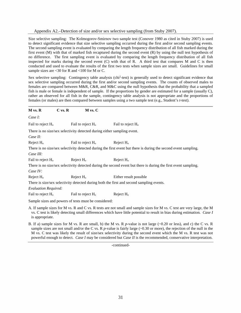
Appendix A2.–Detection of size and/or sex selective sampling (from Stuby 2007).
Size selective sampling: The Kolmogorov-Smirnov two sample test (Conover 1980 as cited in Stuby 2007) is used to detect significant evidence that size selective sampling occurred during the first and/or second sampling events. The second sampling event is evaluated by comparing the length frequency distribution of all fish marked during the first event (M) with that of marked fish recaptured during the second event (R) by using the null test hypothesis of no difference. The first sampling event is evaluated by comparing the length frequency distribution of all fish inspected for marks during the second event (C) with that of R. A third test that compares M and C is then conducted and used to evaluate the results of the first two tests when sample sizes are small. Guidelines for small sample sizes are <30 for R and <100 for M or C.
Sex selective sampling: Contingency table analysis (chi2-test) is generally used to detect significant evidence that sex selective sampling occurred during the first and/or second sampling events. The counts of observed males to females are compared between M&R, C&R, and M&C using the null hypothesis that the probability that a sampled fish is male or female is independent of sample. If the proportions by gender are estimated for a sample (usually C), rather an observed for all fish in the sample, contingency table analysis is not appropriate and the proportions of females (or males) are then compared between samples using a two sample test (e.g., Student’s t-test).
M vs. R C vs. R M vs. C
Case I:
Fail to reject Ho Fail to reject Ho Fail to reject Ho
There is no size/sex selectivity detected during either sampling event. Case II: Reject Ho Fail to reject Ho Reject Ho There is no size/sex selectivity detected during the first event but there is during the second event sampling. Case III: Fail to reject Ho Reject Ho Reject Ho There is no size/sex selectivity detected during the second event but there is during the first event sampling. Case IV: Reject Ho Reject Ho Either result possible There is size/sex selectivity detected during both the first and second sampling events. Evaluation Required: Fail to reject Ho Fail to reject Ho Reject Ho
Sample sizes and powers of tests must be considered:
A. If sample sizes for M vs. R and C vs. R tests are not small and sample sizes for M vs. C test are very large, the M vs. C test is likely detecting small differences which have little potential to result in bias during estimation. Case I is appropriate.
B. If a) sample sizes for M vs. R are small, b) the M vs. R p-value is not large (~0.20 or less), and c) the C vs. R sample sizes are not small and/or the C vs. R p-value is fairly large (~0.30 or more), the rejection of the null in the M vs. C test was likely the result of size/sex selectivity during the second event which the M vs. R test was not powerful enough to detect. Case I may be considered but Case II is the recommended, conservative interpretation.
-continued-
32
Appendix A2.–Page 2 of 2.
C. If a) sample sizes for C vs. R are small, b) the C vs. R p-value is not large (~0.20 or less), and c) the M vs. R sample sizes are not small and/or the M vs. R p-value is fairly large (~0.30 or more), the rejection of the null in the M vs. C test was likely the result of size/sex selectivity during the first event which the C vs. R test was not powerful enough to detect. Case I may be considered but Case III is the recommended, conservative interpretation.
D. If a) sample sizes for C vs. R and M vs. R are both small, and b) both the C vs. R and M vs. R p-values are not large (~0.20 or less), the rejection of the null in the M vs. C test may be the result of size/sex selectivity during both events which the C vs. R and M vs. R tests were not powerful enough to detect. Cases I, II, or III may be considered but Case IV is the recommended, conservative interpretation.
Case I. Abundance is calculated using a Petersen-type model from the entire data set without stratification. Composition parameters may be estimated after pooling length, sex, and age data from both sampling events. Case II. Abundance is calculated using a Petersen-type model from the entire data set without stratification. Composition parameters may be estimated using length, sex, and age data from the first sampling event without stratification. If composition is estimated from second event data or after pooling both sampling events, data must first be stratified to eliminate variability in capture probability (detected by the M vs. R test) within strata. Composition parameters are estimated within strata, and abundance for each stratum needs to be estimated using a Petersen-type formula. Overall composition parameters are estimated by combining stratum estimates weighted by estimated stratum abundance according to the formulae below.
Case III. Abundance is calculated using a Petersen-type model from the entire data set without stratification. Composition parameters may be estimated using length, sex, and age data from the second sampling event without stratification. If composition is estimated from first event data or after pooling both sampling events, data must first be stratified to eliminate variability in capture probability (detected by the C vs. R test) within strata. Composition parameters are estimated within strata, and abundance for each stratum needs to be estimated using a Petersen-type type formula. Overall composition parameters are estimated by combining stratum estimates weighted by estimated stratum abundance according to the formulae below.
Case IV. Data must be stratified to eliminate variability in capture probability within strata for at least one or both sampling events. Abundance is calculated using a Petersen-type model for each stratum, and estimates are summed across strata to estimate overall abundance. Composition parameters may be estimated within the strata as determined above, but only using data from sampling events where stratification has eliminated variability in capture probabilities within strata. If data from both sampling events are to be used, further stratification may be necessary to meet the condition of capture homogeneity within strata for both events. Overall composition parameters are estimated by combining stratum estimates weighted by estimated stratum abundance. If stratification by sex or length is necessary prior to estimating composition parameters, then an overall composition parameters (pk) is estimated by combining within stratum composition estimates using:
∑= Σ
=j
iik
ik p̂
N̂N̂p̂
1; and, (1)
[ ] [ ] [ ]
+≈ ∑ −
=ΣN̂V̂p̂p̂p̂V̂N̂N̂
p̂V̂ i
j
ikikikik )(
1
222
1 . (2)
where: j = the number of sex/size strata; pikˆ = the estimated proportion of fish that were age or size k among fish in stratum i;