20th century trends and budget implications of chloroform and ...

Atmos. Chem. Phys., 6, 2847–2863, 2006www.atmos-chem-phys.net/6/2847/2006/© Author(s) 2006. This work is licensedunder a Creative Commons License.

AtmosphericChemistry

and Physics

20th century trends and budget implications of chloroform andrelated tri-and dihalomethanes inferred from firn air

D. R. Worton1, W. T. Sturges1, J. Schwander2, R. Mulvaney3, J.-M. Barnola4, and J. Chappellaz4

1School of Environmental Sciences, University of East Anglia, Norwich, UK2Physics Institute, University of Berne, Berne, Switzerland3British Antarctic Survey, Natural Environment Research Council, Cambridge, UK4CNRS Laboratoire de Glaciologie et Geophysique de l’Environnement, Saint Martin d’Heres, France

Received: 15 November 2005 – Published in Atmos. Chem. Phys. Discuss.: 24 January 2006Revised: 11 May 2006 – Accepted: 31 May 2006 – Published: 12 July 2006

Abstract. Four trihalomethane (THM; CHCl3, CHBrCl2,CHBr2Cl and CHBr3) and two dihalomethane (DHM;CH2BrCl and CH2Br2) trace gases have been measured inair extracted from polar firn collected at the North Green-land Icecore Project (NGRIP) site. CHCl3 was also mea-sured in firn air from Devon Island (DI), Canada, DronningMaud Land (DML), Antarctica and Dome Concordia (DomeC), Antarctica. All of these species are believed to be al-most entirely of natural origin except for CHCl3 where an-thropogenic sources have been reported to contribute∼10%to the global burden. A 2-D atmospheric model was run forCHCl3 using reported emission estimates to produce histori-cal atmospheric trends at the firn sites, which were then inputinto a firn diffusion model to produce concentration depthprofiles that were compared against the measurements. Theanthropogenic emissions were modified in order to give thebest model fit to the firn data at NGRIP, Dome C and DML.As a result, the contribution of CHCl3 from anthropogenicsources, mainly from pulp and paper manufacture, to the to-tal chloroform budget appears to have been considerably un-derestimated and was likely to have been close to∼50% atthe maximum in atmospheric CHCl3 concentrations around1990, declining to∼29% at the beginning of the 21st century.We also show that the atmospheric burden of the brominatedTHM’s in the Northern Hemisphere have increased over the20th century while CH2Br2 has remained constant over timeimplying that it is entirely of natural origin.

1 Introduction

Halogens play an important role in the chemistry of both thetroposphere and the stratosphere. In the polar troposphere,bromine chemistry has been implicated as the major cause

Correspondence to:D. R. Worton([email protected])

of surface polar ozone depletion (Barrie et al., 1988; Berget al., 1984; Cicerone et al., 1988) and bromine monoxide(BrO) as the major atmospheric oxidant driving mercury de-position (Ariya et al., 2004; Ebinghaus et al., 2002; Lindberget al., 2002; Schroeder et al., 1998). The bromine result-ing from the degradation of short lived bromocarbons hasbeen implicated as a possible initiator for the autocatalyticactivation and recycling of inorganic halogens from sea saltaerosols causing the observed “bromine explosion” events(Foster et al., 2001; Platt and Honninger, 2003; Sander et al.,2003; Vogt et al., 1999). It has been suggested that BrO maynot be constrained to polar regions but could be widespreadthroughout the troposphere where it could influence the HOx

and NOx cycles as well as providing a significant sink fordimethyl sulphide (von Glasow et al., 2004).

In the stratosphere, bromine can deplete ozone with higherefficiency than chlorine,∼45 times (Daniel et al., 1999), andthe dominant sources are understood to be from the photo-chemical degradation of methyl bromide (CH3Br) and thelong lived halon (bromofluorocarbon) compounds. How-ever, recently there is increasing evidence to suggest thatother short lived bromocarbon species (CHBr3, CH2Br2,CH2BrCl, CHBr2Cl, CHBrCl2, C2H5Br and C2H4Br2) couldbe important source gases of stratospheric bromine. Simul-taneous observations of several of these bromocarbons andBrO in the upper troposphere have been reported (Pfeil-sticker et al., 2000), along with several aircraft (Schauffleret al., 1999; Schauffler et al., 1998; Schauffler et al., 1993)and balloon (Kourtidis et al., 1996; Pfeilsticker et al., 2000;Sturges et al., 2000) studies that have shown that these bro-mocarbons are present at concentrations in the part per tril-lion by volume (pptv) range and together are reported tocontribute∼10–15% to the total organic bromine measuredin the upper troposphere lower stratosphere (UTLS) region(Pfeilsticker et al., 2000; Sturges et al., 2000). It has furtherbeen suggested that a fraction of the inorganic bromine orig-inating from the tropospheric breakdown of the same short

Published by Copernicus GmbH on behalf of the European Geosciences Union.

2848 D. R. Worton et al.: Trends and budgets of chloroform and related halomethanes from firn air

lived precursors can reach the stratosphere at concentrationsthat can affect ozone levels (Dvortsov et al., 1999; Nielsenand Douglass, 2001; Pfeilsticker et al., 2000; Salawitch etal., 2005).

Chloroform (CHCl3) is the second most abundant organicsource of natural chlorine to the atmosphere after methylchloride and is an important source of tropospheric chlorine.As such it has been one of the subjects of the Reactive Chlo-rine Emissions Inventory (RCEI). CHCl3 is only estimated tocontribute∼2 Gg CHCl3/yr or <10 pptv (Keene et al., 1999;McCulloch, 2003) to stratospheric chlorine as a result of itsshort tropospheric lifetime of 0.41 years (Ko et al., 2003)relative to other more persistent chlorine containing sourcegases. CHCl3 is degraded in the troposphere, through oxi-dation by OH, to phosgene (COCl2) a small percentage ofwhich reaches the stratosphere where it can participate inozone destruction (Kindler et al., 1995). Chlorine radicalsderived from the atmospheric degradation of CHCl3 can re-act with other organic gases, e.g., hydrocarbons and alkylnitrates, in the troposphere similar to the OH radical. Thiscan affect the tropospheric lifetimes of these species as wellas influencing the local atmospheric composition, especiallyin the polar regions. In the case of hydrocarbons and alkyl ni-trates the rates of reaction with chlorine radicals are greatlyenhanced over those of OH oxidation (IUPAC, 2002; Muthu-ramu et al., 1994 and references therein).

The global tropospheric bromine loading has been re-ported to have peaked in 1998 and to have since declined byapproximately 5% or∼0.8 ppt (Montzka et al., 2003). How-ever, this decrease is reportedly driven by the reduction in at-mospheric methyl bromide and the contributions of the veryshort lived bromocarbons are considered to have remainedconstant (Montzka et al., 2003) as they are generally assumedto be almost entirely of natural origin.

Recently, Sturges et al. (2001) found no evidence for anysignificant temporal trends in the Southern Hemisphere con-centrations of these bromocarbon gases. There are cur-rently no published Northern Hemisphere trends of bromi-nated trace gases as previous firn air studies of these speciesand CH3Br at Devon Island, Canada (Sturges et al., 2001)and CH3Br at Tunu, Greenland (Butler et al., 1999) resultedin the observation of anomalous profiles within the firn thatwere interpreted as having been affected by post depositionalprocesses.

In this work we present the first unperturbed firn profilesof four trihalomethanes (CHBr3, CHBr2Cl, CHBrCl2 andCHCl3) for the Northern Hemisphere from firn air collectedat North GReenland Icecore Project (NGRIP), Greenland.The anthropogenic contribution to the CHCl3 budget is as-sessed using a 2-D model and constrained using firn air mea-surements from Arctic (NGRIP) and Antarctic (Dome Con-cordia and Dronning Maud Land) sites. The implications forthe budgets of the other THM’s are also considered based onthe observed variations in the NGRIP firn air.

2 Sampling and analysis

2.1 Firn air measurements

Firn air samples were collected at the North GreenlandIcecore Project (NGRIP), Greenland (75◦ N, 42◦ W), De-von Island (DI), Canada (75◦ N, 82◦ W), Dronning MaudLand (DML), Antarctica (77◦ S, 10◦ W) and Dome Concor-dia (Dome C), Antarctica (75◦ S, 123◦ E) sites. Details ofthe NGRIP (Reeves et al., 2005) Devon Island, Dome Cand DML sites (Sturges et al., 2001), sampling procedures(Schwander et al., 1993; Sturges et al., 2001) and analyti-cal methodologies (Fraser et al., 1999; Oram et al., 1995;Sturges et al., 2001) have been given elsewhere.

In brief, aliquots of the firn air samples (∼400 ml) werecryogenically concentrated using liquid argon, then desorbedand separated on a DB-5 capillary column (J&W, 60 m) priorto detection by single ion mode mass spectrometry (Micro-mass Autospec) with detection limits of∼0.001 pptv. Theassociated experimental uncertainties, as illustrated by theerror bars in subsequent figures, were determined as the to-tal analytical precision through duplicate analyses of samplesat each depth and the measurement precision of the runningstandard. CHCl3 measurements are presented from all fourfirn sites whereas the brominated tri- and dihalomethanes areonly presented for the NGRIP site. The brominated specieshave also been measured at the other three sites and werereported previously by Sturges et al. (2001).

2.2 Firn modelling

A firn physical transport model that accounts for gravita-tional fractionation and gaseous diffusion (Rommelaere etal., 1997) was employed to interpolate atmospheric trendsinto firn concentration depth profiles. The required tortu-osity profile was determined by inverse modelling of theCO2 profile (Fabre et al., 2000). Diffusion coefficients ofother molecules relative to CO2 were estimated from Le Basmolecular volumes (Fuller et al., 1966). Thermal fractiona-tion effects were not included in the model.

2.3 Atmospheric model

Temporal trends in atmospheric concentrations for the loca-tions of the firn sites were generated using a 2-D atmosphericchemistry transport model. Details of the model are given inReeves (2003). The model contains 18 equal area latitudi-nal bands and 6 vertical layers, each of 2.5 km. The oceancomponent of the 2-D model was removed as the lifetime ofCHCl3 with respect to loss to the ocean has been reported tobe insignificant (Kindler et al., 1995; Yvon-Lewis and But-ler, 2002) relative to the∼0.41 year lifetime resulting fromthe reaction with OH (Ko et al., 2003). Other sink terms in-cluding dry deposition and loss to soils were also removed asthe reaction with OH was considered to be the dominant loss

Atmos. Chem. Phys., 6, 2847–2863, 2006 www.atmos-chem-phys.net/6/2847/2006/

D. R. Worton et al.: Trends and budgets of chloroform and related halomethanes from firn air 2849

process (Keene et al., 1999; McCulloch, 2003). The strato-spheric lifetime of CHCl3 has been estimated at 3.18 years(Kindler et al., 1995) and this was used to determine the dif-fusive loss term out of the uppermost layer of the model.

3 Results and discussion

3.1 Firn depth profiles

3.1.1 CHCl3

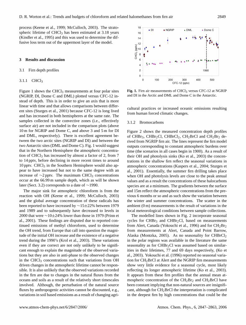
Figure 1 shows the CHCl3 measurements at four polar sites(NGRIP, DI, Dome C and DML) plotted versus CFC-12 in-stead of depth. This is in order to give an axis that is morelinear with time and that allows comparisons between differ-ent sites (Sturges et al., 2001) because CFC-12 is long livedand has increased in both hemispheres at the same rate. Thesamples collected in the convective zones (i.e., effectivelysurface air) are not included in the comparison plots (above10 m for NGRIP and Dome C, and above 3 and 5 m for DIand DML, respectively). There is excellent agreement be-tween the two arctic sites (NGRIP and DI) and between thetwo Antarctic sites (DML and Dome C). Fig. 1 would suggestthat in the Northern Hemisphere the atmospheric concentra-tion of CHCl3 has increased by almost a factor of 2, from 7to 14 pptv, before declining in more recent times to around10 pptv. CHCl3 in the Southern Hemisphere would also ap-pear to have increased but not to the same degree with anincrease of∼2 pptv. The maximum CHCl3 concentrationsoccur at the 66.99 m sample depth, which as will be shownlater (Sect. 3.2) corresponds to a date of∼1990.

The major sink for atmospheric chloroform is from thereaction with OH (Keene et al., 1999; McCulloch, 2003)and the global average concentration of these radicals hasbeen reported to have increased by∼15±22% between 1979and 1989 and to subsequently have decreased to levels in2000 that were∼10±24% lower than those in 1979 (Prinn etal., 2001). These findings are disputed due to reported con-tinued emissions of methyl chloroform, used to determinethe OH trend, from Europe that call into question the magni-tude of the initial OH increase and the existence of a negativetrend during the 1990’s (Krol et al., 2003). These variationseven if they are correct are not only unlikely to be signifi-cant enough to explain the magnitude of the observed varia-tions but they are also in anti-phase to the observed changesin the CHCl3 concentrations such that variations from OHdriven changes in the atmospheric lifetime cannot be respon-sible. It is also unlikely that the observed variations recordedin the firn are due to changes in the natural fluxes from theoceans and soils as a result of the relatively short timescalesinvolved. Although, the perturbation of the natural sourcefluxes by anthropogenic activities cannot be discounted, e.g.,variations in soil based emissions as a result of changing agri-

Fig. 1. Firn air measurements of CHCl3 versus CFC-12 at NGRIPand DI in the Arctic and DML and Dome C in the Antarctic.

cultural practices or increased oceanic emissions resultingfrom human forced climatic changes.

3.1.2 Bromocarbons

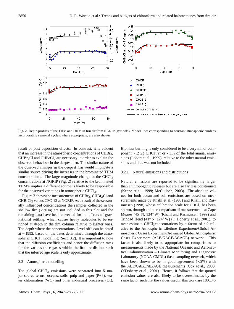
Figure 2 shows the measured concentration depth profilesof CHBr3, CHBr2Cl, CHBrCl2, CH2BrCl and CH2Br2 de-rived from NGRIP firn air. The lines represent the firn modeloutputs corresponding to constant atmospheric burdens overtime (the scenarios in all cases begin in 1900). As a result oftheir OH and photolysis sinks (Ko et al., 2003) the concen-trations in the shallow firn reflect the seasonal variations inatmospheric concentrations (Kaspers et al., 2004; Sturges etal., 2001). Essentially, the summer firn drilling takes placewhen OH and photolysis levels are close to the peak annualvalues and as a result the concentrations of these halocarbonsspecies are at a minimum. The gradients between the surfaceand 15m reflect the atmospheric concentrations from the pre-vious 6 months or so and as such show the variation betweenthe winter and summer concentrations. The scatter in theambient (0 m) measurements is the result of variations in thelocal meteorological conditions between sample collections.

The modelled lines shown in Fig. 2 incorporate seasonalcycles for CHBr3 and CHBr2Cl, based on measurementsfrom Alert, Canada (Yokouchi et al., 1996) and for CH2Br2from measurements at Alert, Canada and Point Barrow,Alaska (Montzka, 2005). As no seasonality for CHBrCl2in the polar regions was available in the literature the sameseasonality as for CHBr2Cl was assumed based on similar-ities in their lifetimes, 77 and 69 days respectively, (Ko etal., 2003). Yokouchi et al. (1996) reported no seasonal varia-tion for CH2BrCl at Alert and the NGRIP firn measurementsshow very little evidence for a seasonal cycle, most likelyreflecting its longer atmospheric lifetime (Ko et al., 2003).It appears from these firn profiles that the annual mean at-mospheric concentration of the CH2Br2 and CH2BrCl havebeen constant implying that non-natural sources are insignifi-cant, although for CH2BrCl the interpretation is complicatedin the deepest firn by high concentrations that could be the

www.atmos-chem-phys.net/6/2847/2006/ Atmos. Chem. Phys., 6, 2847–2863, 2006


Fig. 2. Depth profiles of the THM and DHM in firn air from NGRIP (symbols). Model lines corresponding to constant atmospheric burdensincorporating seasonal cycles, where appropriate, are also shown.

result of post deposition effects. In contrast, it is evidentthat an increase in the atmospheric concentrations of CHBr3,CHBr2Cl and CHBrCl2 are necessary in order to explain theobserved behaviour in the deepest firn. The similar nature ofthe observed changes in the deepest firn would implicate asimilar source driving the increases in the brominated THMconcentrations. The large magnitude change in the CHCl3concentrations at NGRIP (Fig. 2) relative to the brominatedTHM’s implies a different source is likely to be responsiblefor the observed variations in atmospheric CHCl3.

Figure 3 shows the measurements of CHBr3, CHBr2Cl andCHBrCl2 versus CFC-12 at NGRIP. As a result of the season-ally influenced concentrations the samples collected in theshallow firn (<30 m) are not included in this plot and theremaining data have been corrected for the effects of grav-itational settling, which causes heavy molecules to be en-riched at depth in the firn column relative to lighter ones.The depth where the concentrations “level off” can be datedat ∼1992, based on the dates determined through the atmo-spheric CHCl3 modelling (Sect. 3.2). It is important to notethat the diffusion coefficients and hence the diffusion ratesfor the various trace gases within the firn are distinct suchthat the inferred age scale is only approximate.

3.2 Atmospheric modelling

The global CHCl3 emissions were separated into 5 ma-jor source terms; oceans, soils, pulp and paper (P+P), wa-ter chlorination (WC) and other industrial processes (OI).

Biomass burning is only considered to be a very minor com-ponent,<2 Gg CHCl3/yr or <1% of the total annual emis-sions (Lobert et al., 1999), relative to the other natural emis-sions and thus was not included.

3.2.1 Natural emissions and distributions

Natural emissions are reported to be significantly largerthan anthropogenic releases but are also far less constrained(Keene et al., 1999; McCulloch, 2003). The absolute val-ues for both ocean and soil emissions are based on mea-surements made by Khalil et al. (1983) and Khalil and Ras-mussen (1998) whose calibration scale for CHCl3 has beenshown, through an intercomparison of measurements at CapeMeares (45◦ N, 124◦ W) (Khalil and Rasmussen, 1999) andTrindad Head (41◦ N, 124◦ W) (O’Doherty et al., 2001), toover estimate CHCl3concentrations by a factor of∼2 rel-ative to the Atmospheric Lifetime Experiment/Global At-mospheric Gases Experiment/Advanced Global AtmosphericGases Experiment (ALE/GAGE/AGAGE) network. Thisfactor is also likely to be appropriate for comparisons tomeasurements made by the National Oceanic and Aeronau-tical Administration – Climate Monitoring and DiagnosticLaboratory (NOAA-CMDL) flask sampling network, whichhave been shown to be in good agreement (<5%) withthe ALE/GAGE/AGAGE measurements (Cox et al., 2003;O’Doherty et al., 2001). Hence, it follows that the quotedemission values are also likely to be overestimates by thesame factor such that the values used in this work are 180±45



Fig. 3. Gravity corrected firn air measurements of CHBr3,CHBr2Cl and CHBrCl2 versus CFC-12 at NGRIP.

and 100+100/–50 Gg CHCl3/yr for oceans and soils, respec-tively, i.e.,∼50% lower than those values reported by Khalilet al. (1999).

As a result of the significant reported uncertainties in thenatural emission magnitudes and a lack of information con-cerning the likely source distributions, the RCEI did not at-tempt to estimate the latitudinal distribution. Nevertheless aspart of the RCEI’s work (Khalil et al., 1999) the ocean andsoil emissions were constrained into 4 latitudinal bands; 0–30◦, 30–90◦ for each hemisphere. In order to incorporate thenatural emissions into our model it was necessary to estimatethe distribution of the natural sources on a finer scale (i.e.,18 latitudinal boxes). This was achieved by assuming thatthe flux rates per unit area within these bands are uniformlydistributed. The latitudinal distribution of natural emissionsfrom this very simple approach, from now on referred to asND1, is shown in Fig. 4.

A second approach was aimed at developing this firstapproximation into a more smoothed distribution. Thisapproach involved determining emission factors for theocean and soils based on their fractional global coverageGross (1972), which was used in conjunction with the as-sumption that the tropical oceans (≤30◦) are more produc-tive than the sub tropics (>30◦) and that this relationship waslinear with latitude, i.e., increasing linearly towards the equa-tor. This assumption is supported in essence by the greateremissions reported at lower latitudes by Khalil et al. (1999),although the linearity of the relationship is based on specula-tion only. For the soils, they were assumed to cover all areasthat were not classified as oceans (Gross, 1972) and the emis-sion factor was assumed to be independent of latitude andthus constant for the entire globe. This assumption is clearlylimited since there are large differences in soil and landscapetypes. Soil emissions from the most southerly box were setto zero since the only land mass<60◦ S is Antarctica. How-ever, due to the resolution of the model, it was not possibleto assume the same for the most northerly box because there

Fig. 4. The two estimated natural distributions (ND1= natural dis-tribution 1, ND2 = natural distribution 2 as defined in Sect. 3.2.1)used within this 2-D modelling work. The x-axis represents the lat-itude with positive values reflecting the Northern Hemisphere andnegative values the Southern Hemisphere.

is not a permanent icesheet covering all land masses>60◦ N.To obtain a distribution that fitted within the constraints of

all these parameters it was necessary to use individual nor-malisation factors for both the oceans and the soils to correctthe calculated figures within each of the 4 larger semi hemi-spheric bands to match those reported by Khalil et al. (1999).All of these applied normalisation factors were 1.0±0.1 giv-ing good confidence for the calculated figures and for com-parisons between the individual model boxes. It should benoted that the applied soil emission factors>33◦ S, i.e. inthe most southerly semi-hemisphere, are higher by a factorof ∼2.6 than for all other latitudes. This appears to be nec-essary in order to match the estimated emissions of Khalilet al. (1999) without requiring a large normalisation factor.Since land accounts for only 0.2 to 7.4% of the surface areain these boxes, this has a negligible effect on the overall bud-get. This distribution, from now referred to as ND2, is shownin Fig. 4.

3.2.2 Anthropogenic distributions and trends

In the literature, the estimated anthropogenic sourcestrengths of CHCl3 are reportedly small (Aucott et al., 1999)relative to the estimated natural emissions (Khalil etal., 1999). The associated uncertainties reported (Aucott etal., 1999; Khalil et al., 1999) with these estimates wouldsuggest that the anthropogenic source strength is better con-strained and hence more well known although this work, aswill be shown, would suggest that this is unlikely to be cor-rect. As part of the RCEI work a global 1◦

×1◦ grided inven-tory of anthropogenic CHCl3 emissions was produced basedon 1990 estimates (Aucott et al., 1999). The 3 Gg CHCl3/yremissions resulting from combustion sources, landfills andruminants were not included in the grided inventory as theywere considered to be too small to make a significant im-pact (Aucott et al., 1999). As emissions were given as mass



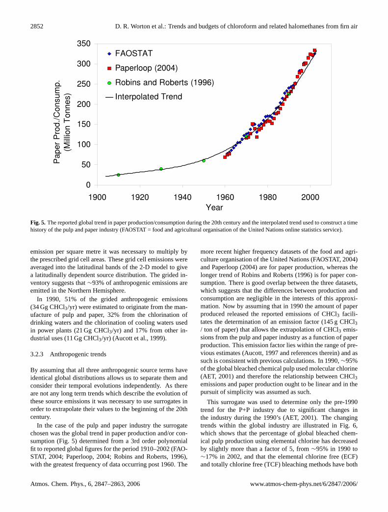
Fig. 5. The reported global trend in paper production/consumption during the 20th century and the interpolated trend used to construct a timehistory of the pulp and paper industry (FAOSTAT = food and agricultural organisation of the United Nations online statistics service).

emission per square metre it was necessary to multiply bythe prescribed grid cell areas. These grid cell emissions wereaveraged into the latitudinal bands of the 2-D model to givea latitudinally dependent source distribution. The grided in-ventory suggests that∼93% of anthropogenic emissions areemitted in the Northern Hemisphere.

In 1990, 51% of the grided anthropogenic emissions(34 Gg CHCl3/yr) were estimated to originate from the man-ufacture of pulp and paper, 32% from the chlorination ofdrinking waters and the chlorination of cooling waters usedin power plants (21 Gg CHCl3/yr) and 17% from other in-dustrial uses (11 Gg CHCl3/yr) (Aucott et al., 1999).

3.2.3 Anthropogenic trends

By assuming that all three anthropogenic source terms haveidentical global distributions allows us to separate them andconsider their temporal evolutions independently. As thereare not any long term trends which describe the evolution ofthese source emissions it was necessary to use surrogates inorder to extrapolate their values to the beginning of the 20thcentury.

In the case of the pulp and paper industry the surrogatechosen was the global trend in paper production and/or con-sumption (Fig. 5) determined from a 3rd order polynomialfit to reported global figures for the period 1910–2002 (FAO-STAT, 2004; Paperloop, 2004; Robins and Roberts, 1996),with the greatest frequency of data occurring post 1960. The

more recent higher frequency datasets of the food and agri-culture organisation of the United Nations (FAOSTAT, 2004)and Paperloop (2004) are for paper production, whereas thelonger trend of Robins and Roberts (1996) is for paper con-sumption. There is good overlap between the three datasets,which suggests that the differences between production andconsumption are negligible in the interests of this approxi-mation. Now by assuming that in 1990 the amount of paperproduced released the reported emissions of CHCl3 facili-tates the determination of an emission factor (145 g CHCl3/ ton of paper) that allows the extrapolation of CHCl3 emis-sions from the pulp and paper industry as a function of paperproduction. This emission factor lies within the range of pre-vious estimates (Aucott, 1997 and references therein) and assuch is consistent with previous calculations. In 1990,∼95%of the global bleached chemical pulp used molecular chlorine(AET, 2001) and therefore the relationship between CHCl3emissions and paper production ought to be linear and in thepursuit of simplicity was assumed as such.

This surrogate was used to determine only the pre-1990trend for the P+P industry due to significant changes inthe industry during the 1990’s (AET, 2001). The changingtrends within the global industry are illustrated in Fig. 6,which shows that the percentage of global bleached chem-ical pulp production using elemental chlorine has decreasedby slightly more than a factor of 5, from∼95% in 1990 to∼17% in 2002, and that the elemental chlorine free (ECF)and totally chlorine free (TCF) bleaching methods have both



Fig. 6. The changing trend in the bleaching methods; elementalchlorine, elemental chlorine free (ECF) and totally chlorine free(TCF), used in the pulp and paper industry during the 1990’s (AET,2001).

increased over the same time frame, from 5% to 68% and0.2% to 6.5%, respectively (AET, 2001). These changingtrends are reflected, for the United States of America (USA)at least, by significant reductions (∼86%) in the air emis-sions of CHCl3 from the P+P industry (USEPA, 2004). Thisdeclining trend was well approximated (R2=0.98) by a 2ndorder polynomial function, which was used in all further cal-culations. The decline in the USA’s use of elemental chlo-rine in pulp production is shown (Fig. 7) to be well corre-lated (R2=+0.74) with the global decrease (AET, 2001). Thiscorrelation suggests that it is reasonable to assume that theobserved decrease in CHCl3 emissions from the USA P+Pindustry (USEPA, 2004) also reflects what has been occur-ring on a global scale. This is a reasonably quantitative as-sumption since the USA’s P+P production has accounted for≥30–60% of world production over the last 40 years (Paper-loop, 2004). These approximations were used to determinethe declining trend in CHCl3 emissions from the global P+Pindustry for the period 1990–2002 and combined with thesurrogate trend based on paper production and consumptionfigures to give an estimation of the 20th century emissionhistory.

The global population was used as a surrogate for WCand OI processes and was based on the assumption that withan increasing population comes an increasing demand anduse of chlorinated drinking water and an increasing demandfor electricity and hence a likely increase in the amount ofcooling water chlorinated for use in power stations. The in-creasing global population is also likely to reflect the addi-tional demands of an industrialising society that are consid-ered as part of the other industrial processes by the RCEI.The global population has been used previously as a surro-gate for anthropogenic CHCl3 emissions (Trudinger et al.,2004) and this trend was determined from population figuresabove the 1920 population, hence fixing a timeframe for zeroemissions. The chlorination of water began at the turn of

Fig. 7. The relationship between the use of elemental chlorine dur-ing the bleaching of paper pulp in the United States of America(USA) and the rest of the world.

the century and became widespread by 1920 (AWWA, 2004)suggesting a reasonable approximation for zero emissions.

The global population trend was determined from datapublished by the United Nations (UN, 2004) and the Popula-tion Reference Bureau (Ashford et al., 2004) with the higherfrequency data occurring post 1950. It was necessary to as-sume a linear growth rate between 1900 and 1950 due to lackof data. A surrogate global population trend was devised bycorrecting to population figures above that of 1920. Now byassuming that in 1990 the reported releases of CHCl3 for thewater chlorination and other industrial processes categorieswere associated with the surrogate population at that time al-lows the determination of emission factors, 6.28 and 3.34 GgCHCl3 / billion people for water chlorination and other in-dustrial processes, respectively. These emission factors allowthe determination of CHCl3 emissions from these industriesas a function of the global population.

The temporal variations, over a 100 year period, for allsource terms, including a trend that incorporates a changingsoil source (Sect. 3.2.4), are shown in Fig. 8. A critical as-sumption is that the natural emissions from oceans and soilshave not changed over this time frame. We concede that in-creased emissions from the biosphere could have taken placeduring the 20th century, e.g., as a result of increasing globaltemperatures. However, there is scant evidence to supportsuch increases as a result of the apparent lack of increasingtrends in the THM and DHM measurements in the South-ern Hemisphere (Sturges et al., 2001) and the DHMs in theNorthern Hemisphere (this work). The largest changes occurin the Northern Hemisphere and since it is hard to imaginea natural source that only operates in one hemisphere a largevariation in the anthropogenic emissions needs to be invokedto describe the observations. An inherent assumption withthis approach is that the latitudinal distribution of all sourceterms has remained constant over time.



Fig. 8. The time trends over the 20th century for all the natural andanthropogenic source components (1SS = changing soil source;P+P = pulp and paper; WC = water chlorination; OI = other in-dustries) incorporated in the modelling.

3.2.4 Varying the soil source as function of population

To reconcile their modelling results, Trudinger et al. (2004)hypothesise that the soil source may have increased with timeas a result of agricultural interference. This is supportedby a recent report that suggests that the amount of land be-ing cultivated has increased substantially in recent times andthat since 1940 the amount of land turned over to agriculturewas larger than in the two previous centuries combined (UN,2005). However, the notion that cultivated soil emits moreCHCl3 than uncultivated soils is one of speculation and thereis no supporting evidence for this at the current time.

To investigate Trudinger et al.’s suggestion of an increas-ing soil source, the soil emissions were fixed at 100 GgCHCl3 for 1990 and extrapolated back to the beginning ofthe century as a function of the global population in the sameway as was performed for the WC and OI temporal varia-tions. This trend is referred to from now on as the chang-ing soil source (1SS) and is shown in Fig. 8. The effect ofconstant soil and changing soil emissions are discussed inSect. 3.2.5. It is apparent that a much smaller variation inthe natural emissions (e.g., soils) would be needed relativeto any changes in the anthropogenic emissions to affect thesame magnitude change in the concentrations observed at theAntarctic sites, as a result of the northern mid latitude bias ofthe anthropogenic distribution.

3.2.5 Varying the magnitude of anthropogenic emissions

The reported (Aucott 1997) uncertainty levels associatedwith each of the anthropogenic source terms suggest that thereported values (Aucott et al., 1999) could be up to a fac-tor of 2 larger. Therefore, all the anthropogenic emissionswere doubled, which resulted in a better approximation tothe NGRIP data (Fig. 9). The changing soil source (1SS)

Fig. 9. A comparison of the effect of varying the magnitude of allanthropogenic sources (x1 = reactive chlorine emissions inventory(RCEI) figures as reported by Aucott et al. (1999); x2=double thereported RCEI figures; x2+1SS = double the RCEI figures pluschanging soil source) with the NGRIP firn air measurements ofCHCl3.

scenario is also shown in Fig. 9 and the effects observed atNGRIP are reasonably small with slightly lower values beingmodelled in the deeper part of the profile whilst the oppositeis apparent for the near surface. The effect of this scenariois more significant for the Southern Hemisphere sites (notshown) where the higher values in the shallow firn and lowervalues in the deeper firn appear to improve the fit to the mea-surements. However, these improved fits are more likely re-flecting the consequence of the distribution of soil coveragewithin the model as opposed to a definitive anthropogenicperturbation.

It is evident from Fig. 9 that the magnitude of the anthro-pogenic emissions required to fully capture the maximumvalues observed in the NGRIP firn air measurements stillneeds to be larger than double the reported values. The strongdeclining trend in atmospheric CHCl3 observed at NGRIPcoupled with the proposed source trends would suggest thatonly by further increasing the emissions from the P+P indus-try would it be possible to both model the maximum valuesobserved in the firn while still maintaining a good approxi-mation to the observed decline in the firn between 60 m andthe surface. Several runs were performed to evaluate the sen-sitivity of the model to increases in emissions from the P+Pindustry. During these model runs the natural emissions wereconstrained at a constant value of 280 Gg CHCl3 yr through-out. The magnitude of the WC and OI emissions were fixedat either the reported values (Aucott et al., 1999) or at doublethese values dependent on the particular run. The P+P emis-sions were varied between 3–5 times the value reported byAucott et al. (1999).

The various model outputs are shown in Fig. 10 whereit is clear that too effectively model the near surface



Fig. 10.A comparison of the effect of varying the magnitude of thevarious independent anthropogenic source components (P+P = pulpand paper; WC = water chlorination; OI = other industries) relativeto the NGRIP firn air measurements of CHCl3.

concentrations the emissions from the WC and OI industriesneed to be double those reported in the literature. P+P emis-sions between∼4–5 times the reported values would appearto be necessary to simulate the maximum CHCl3 concentra-tions observed in the firn with the bias being towards the up-per end of this range. We are not alone in believing that theanthropogenic emissions fluxes have been underestimated,Trudinger et al. (2004) also invoked an increase in emissionsfrom anthropogenic sources to model their firn air measure-ments although our magnitude is smaller by comparison. Theconclusions regarding the magnitude of the anthropogenicemissions are based on the assumption that the magnitude ofthe natural emissions are correct. It should be noted that al-though the uncertainties in the natural source terms are fairlylarge, the fact that the concentrations observed at the bottomof the firn at NGRIP where natural emissions account for>90% of the total emissions coupled with the modelled con-centrations for Dome C and DML together suggest that theemission magnitudes are reasonable. The values correspond-ing to the model outputs corresponding to the increased an-thropogenic emissions are shown as latitudinal variations for1990 levels compared against the natural emissions in orderto illustrate the importance of the anthropogenic contributionto the total budget. The largest contribution is in the North-ern Hemisphere mid latitudes where this modelling wouldsuggest that the anthropogenic emissions strongly dominantover the natural emissions (Fig. 11).

3.2.6 Latitudinal variation of peak anthropogenic emis-sions

In order to model the sensitivity of the location of the latitudi-nal maximum peak in the anthropogenic emissions the peakof the emissions was moved north and south while keeping

Fig. 11.A comparison of the latitudinal distribution of the increasedmagnitude of anthropogenic emissions (RCEI = reactive chlorineemissions inventory emission figures as reported by Aucott et al.(1999); P+P = pulp and paper; WC = water chlorination; OI = otherindustries) relative to the distribution of natural emissions (ND2 =natural distribution 2 as defined in Sect. 3.2.1). The x-axis repre-sents the latitude with positive values reflecting the Northern Hemi-sphere and negative values the Southern Hemisphere.

the total emissions constant. The result is four different lati-tudinal distributions shown in Fig. 12. The base case scenarioused to test these latitudinal distributions was with constantnatural emissions, double the reported WC and OI emissions(Aucott et al., 1999) and four times the reported P+P emis-sions (Aucott et al., 1999). As might be expected the locationof the maximum peak in the anthropogenic distribution hasless effect on the modelled trends at sites that are far removedfrom the northern mid latitudes, i.e., DML and Dome C. AtNGRIP (Fig. 13) the dependency is the largest and the con-centrations vary by≤+7.6/-7.1% between peak emissions inbox 2 and boxes 1 and 4, respectively. This approach alsosimulates a difference in transport rates, e.g., moving themaximum peak north simulates a more northerly bias in thetransport, and vice versa, that perhaps is not captured as aresult of the parameterisation of the transport scheme withinthe 2-D model.

It is likely that the anthropogenic distribution used in thiswork is reasonably accurate since, for the majority of the an-thropogenic emissions, the RCEI used the reported addressesof CHCl3 emitting facilities to create their grided inventory.The largest uncertainty associated with the conversion of theRCEI grided inventory into the 2-D model is from the pulpand paper emissions from China and Russia. The location oftheir pulp and paper plants are not known accurately sincethey are not listed in the International Phillips’ 1997 Pa-per Directory (Miller Freeman Information Services 1996),which was used by Aucott et al. (1999) to locate facilitiesin other parts of the world. Instead, the emissions for Chinaand Russia were re-distributed based on population density(Aucott et al., 1999). In the case of China, this issue is com-plicated because its geographical location straddles two of



Fig. 12. The four various anthropogenic distributions used todemonstrate the sensitivity of the model to slight shifts in the lo-cation of the maximum emissions (RCEI = original latitudinal dis-tribution determined from the reported (Aucott et al., 1999) gridedinventory (Sect. 3.2.2); max box 1 = maximum anthropogenic emis-sions in model box 1, i.e., most northerly box; max box 3 = max-imum anthropogenic emissions in model box 3 etc.). The x-axisrepresents the latitude with positive values reflecting the NorthernHemisphere and negative values the Southern Hemisphere.

the model boxes. However, the effects are likely to be smallas China and Russia are responsible for<10% and<5%,respectively, of global pulp and paper production (Johnston,1996).

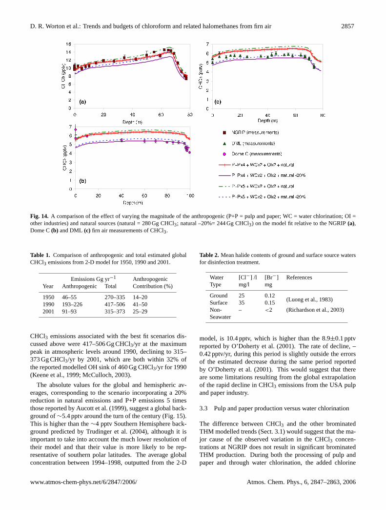
The closest fitting model trends are shown for NGRIP,Dome C and DML in Fig. 14. There are four best fit trendsthat correspond to slightly different emission scenarios, asdefined in the figure legends. The four scenarios shownincorporate either 4 or 5 times the reported P+P emissions(Aucott et al., 1999), double the reported WC and OI emis-sions (Aucott et al., 1999) and either natural emissions of280 Gg or 224 Gg (a reduction of 20%). The reduced nat-ural emissions where introduced to improve the fits to theAntarctic firn air data and are well within the estimated un-certainties reported by Khalil et al. (1999). The total anthro-pogenic emissions associated with these four scenarios are190–230 Gg at the peak in atmospheric CHCl3 around 1990.These anthropogenic emissions are significantly larger thanthe estimated 66 Gg CHCl3 reported by the RCEI (Aucott etal., 1999) and arise as a result of doubling the emissions fromWC and OI and multiplying those from the P+P industry bya factor of 4 or 5. These increases were necessary in orderto capture the magnitude of the variation observed within thefirn air at NGRIP. Invoking more northerly transport wouldslightly reduce the estimated magnitude of these emissions.

This modelling strongly suggests that the reported anthro-pogenic emission estimates are underestimated, especiallyfor the P+P industry. The incorporated values for the WCand OI industries are within the described uncertainties ofbetween a factor of 2 and 5 reported by Aucott (1997). How-

Fig. 13. A comparison of the effect on the model output atNGRIP for the four anthropogenic distributions shown in Fig. 12(RCEI=original latitudinal distribution determined from the re-ported (Aucott et al., 1999) grided inventory Sect. (3.2.2); max box1=maximum anthropogenic emissions in model box 1, i.e., mostnortherly box; max box 3 = maximum anthropogenic emissions inmodel box 3 etc.).

ever, the emission values used for the pulp and paper indus-try are outside the described uncertainties of a factor of 2reported by Aucott (1997). This would suggest that the emis-sion factors determined by Aucott (1997) to extrapolate theglobal emissions from the P+P industry are likely to be un-derestimated and need to be re-evaluated.

At NGRIP, three of the four best fit trends model themeasured maxima well. At Dome C and DML, the trendswhich incorporate natural emissions of 280 Gg over predictthe measurements although the general trend is well simu-lated (Fig. 14). However, reducing the natural emissions by20% to 224 Gg results in significant improvements in themodel fits to the majority of the data except the shallow-est firn where concentrations are slightly under estimated(Fig. 14).

3.2.7 Varying anthropogenic emissions

The contribution of anthropogenic sources to the total globalCHCl3 emissions at the peak in 1990 was likely to have been∼41–50% (Table 1) and is strongly dependent on exactlywhich values are chosen for the natural and anthropogenicemissions. What is clear is that this value is significantlylarger than the∼10–12% previously reported by Khalil etal. (1999) and McCulloch (2003) and slightly lower than the∼60% estimated by Trudinger et al. (2004). This contribu-tion declines between 1990 and 2001 as a result of the re-duced emissions from the P+P industry but is still predictedto be∼25–29% in 2001 (Table 1).

The atmospheric lifetime for CHCl3 determined fromthe model was 0.40.01 years, which is consistent withthat recently reported by Ko et al. (2003). The total



Fig. 14. A comparison of the effect of varying the magnitude of the anthropogenic (P+P = pulp and paper; WC = water chlorination; OI =other industries) and natural sources (natural = 280 Gg CHCl3; natural –20%= 244 Gg CHCl3) on the model fit relative to the NGRIP(a),Dome C(b) and DML (c) firn air measurements of CHCl3.

Table 1. Comparison of anthropogenic and total estimated globalCHCl3 emissions from 2-D model for 1950, 1990 and 2001.

Emissions Gg yr−1 AnthropogenicYear Anthropogenic Total Contribution (%)

1950 46–55 270–335 14–201990 193–226 417–506 41–502001 91–93 315–373 25–29

CHCl3 emissions associated with the best fit scenarios dis-cussed above were 417–506 Gg CHCl3/yr at the maximumpeak in atmospheric levels around 1990, declining to 315–373 Gg CHCl3/yr by 2001, which are both within 32% ofthe reported modelled OH sink of 460 Gg CHCl3/yr for 1990(Keene et al., 1999; McCulloch, 2003).

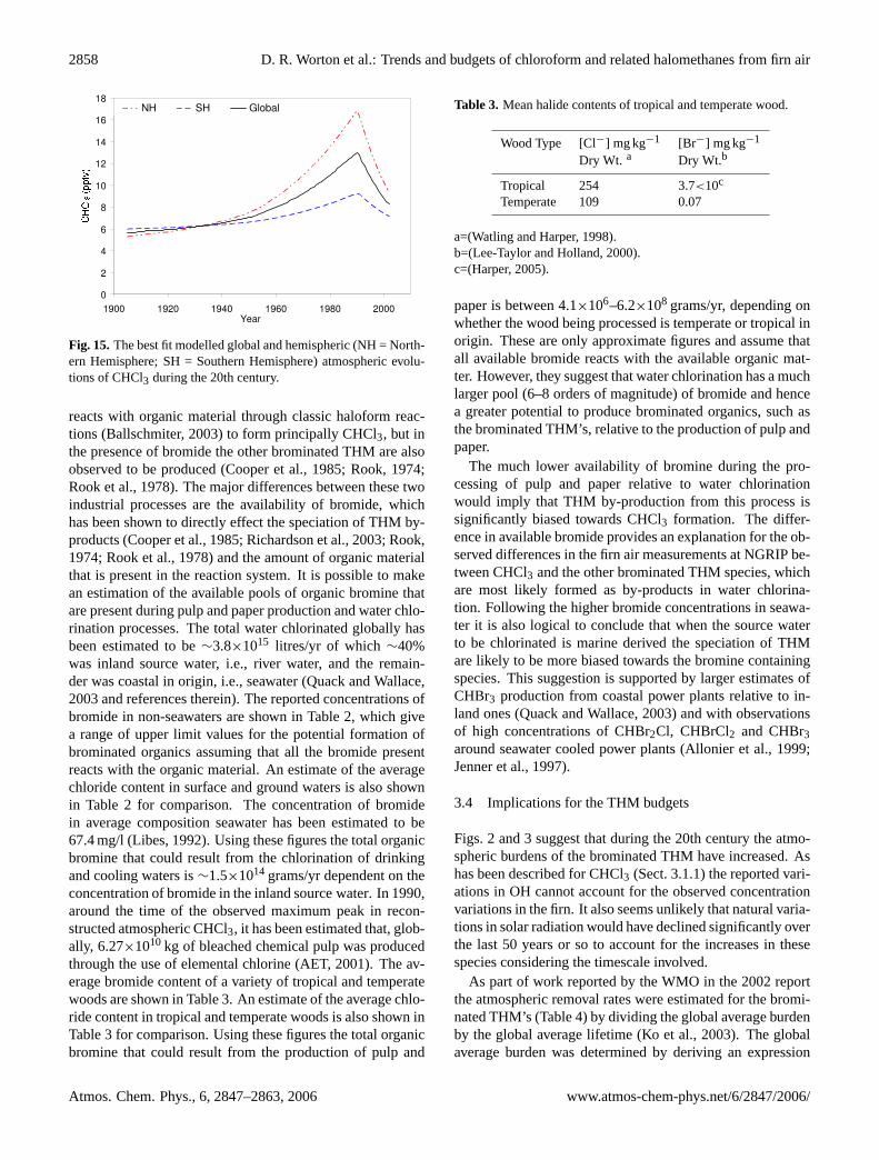
The absolute values for the global and hemispheric av-erages, corresponding to the scenario incorporating a 20%reduction in natural emissions and P+P emissions 5 timesthose reported by Aucott et al. (1999), suggest a global back-ground of∼5.4 pptv around the turn of the century (Fig. 15).This is higher than the∼4 pptv Southern Hemisphere back-ground predicted by Trudinger et al. (2004), although it isimportant to take into account the much lower resolution oftheir model and that their value is more likely to be rep-resentative of southern polar latitudes. The average globalconcentration between 1994–1998, outputted from the 2-D

Table 2. Mean halide contents of ground and surface source watersfor disinfection treatment.

Water [Cl−] /l [Br −] ReferencesType mg/l mg

Ground 25 0.12(Luong et al., 1983)Surface 35 0.15

Non- – <2 (Richardson et al., 2003)Seawater

model, is 10.4 pptv, which is higher than the 8.9±0.1 pptvreported by O’Doherty et al. (2001). The rate of decline, –0.42 pptv/yr, during this period is slightly outside the errorsof the estimated decrease during the same period reportedby O’Doherty et al. (2001). This would suggest that thereare some limitations resulting from the global extrapolationof the rapid decline in CHCl3 emissions from the USA pulpand paper industry.

3.3 Pulp and paper production versus water chlorination

The difference between CHCl3 and the other brominatedTHM modelled trends (Sect. 3.1) would suggest that the ma-jor cause of the observed variation in the CHCl3 concen-trations at NGRIP does not result in significant brominatedTHM production. During both the processing of pulp andpaper and through water chlorination, the added chlorine



Fig. 15.The best fit modelled global and hemispheric (NH = North-ern Hemisphere; SH = Southern Hemisphere) atmospheric evolu-tions of CHCl3 during the 20th century.

reacts with organic material through classic haloform reac-tions (Ballschmiter, 2003) to form principally CHCl3, but inthe presence of bromide the other brominated THM are alsoobserved to be produced (Cooper et al., 1985; Rook, 1974;Rook et al., 1978). The major differences between these twoindustrial processes are the availability of bromide, whichhas been shown to directly effect the speciation of THM by-products (Cooper et al., 1985; Richardson et al., 2003; Rook,1974; Rook et al., 1978) and the amount of organic materialthat is present in the reaction system. It is possible to makean estimation of the available pools of organic bromine thatare present during pulp and paper production and water chlo-rination processes. The total water chlorinated globally hasbeen estimated to be∼3.8×1015 litres/yr of which ∼40%was inland source water, i.e., river water, and the remain-der was coastal in origin, i.e., seawater (Quack and Wallace,2003 and references therein). The reported concentrations ofbromide in non-seawaters are shown in Table 2, which givea range of upper limit values for the potential formation ofbrominated organics assuming that all the bromide presentreacts with the organic material. An estimate of the averagechloride content in surface and ground waters is also shownin Table 2 for comparison. The concentration of bromidein average composition seawater has been estimated to be67.4 mg/l (Libes, 1992). Using these figures the total organicbromine that could result from the chlorination of drinkingand cooling waters is∼1.5×1014 grams/yr dependent on theconcentration of bromide in the inland source water. In 1990,around the time of the observed maximum peak in recon-structed atmospheric CHCl3, it has been estimated that, glob-ally, 6.27×1010 kg of bleached chemical pulp was producedthrough the use of elemental chlorine (AET, 2001). The av-erage bromide content of a variety of tropical and temperatewoods are shown in Table 3. An estimate of the average chlo-ride content in tropical and temperate woods is also shown inTable 3 for comparison. Using these figures the total organicbromine that could result from the production of pulp and

Table 3. Mean halide contents of tropical and temperate wood.

Wood Type [Cl−] mg kg−1 [Br−] mg kg−1

Dry Wt. a Dry Wt.b

Tropical 254 3.7<10c

Temperate 109 0.07

a=(Watling and Harper, 1998).b=(Lee-Taylor and Holland, 2000).c=(Harper, 2005).

paper is between 4.1×106–6.2×108 grams/yr, depending onwhether the wood being processed is temperate or tropical inorigin. These are only approximate figures and assume thatall available bromide reacts with the available organic mat-ter. However, they suggest that water chlorination has a muchlarger pool (6–8 orders of magnitude) of bromide and hencea greater potential to produce brominated organics, such asthe brominated THM’s, relative to the production of pulp andpaper.

The much lower availability of bromine during the pro-cessing of pulp and paper relative to water chlorinationwould imply that THM by-production from this process issignificantly biased towards CHCl3 formation. The differ-ence in available bromide provides an explanation for the ob-served differences in the firn air measurements at NGRIP be-tween CHCl3 and the other brominated THM species, whichare most likely formed as by-products in water chlorina-tion. Following the higher bromide concentrations in seawa-ter it is also logical to conclude that when the source waterto be chlorinated is marine derived the speciation of THMare likely to be more biased towards the bromine containingspecies. This suggestion is supported by larger estimates ofCHBr3 production from coastal power plants relative to in-land ones (Quack and Wallace, 2003) and with observationsof high concentrations of CHBr2Cl, CHBrCl2 and CHBr3around seawater cooled power plants (Allonier et al., 1999;Jenner et al., 1997).

3.4 Implications for the THM budgets

Figs. 2 and 3 suggest that during the 20th century the atmo-spheric burdens of the brominated THM have increased. Ashas been described for CHCl3 (Sect. 3.1.1) the reported vari-ations in OH cannot account for the observed concentrationvariations in the firn. It also seems unlikely that natural varia-tions in solar radiation would have declined significantly overthe last 50 years or so to account for the increases in thesespecies considering the timescale involved.

As part of work reported by the WMO in the 2002 reportthe atmospheric removal rates were estimated for the bromi-nated THM’s (Table 4) by dividing the global average burdenby the global average lifetime (Ko et al., 2003). The globalaverage burden was determined by deriving an expression



Table 4. Estimated lifetimes, removal rates/emission fluxes and associated uncertainties for the three brominated THM in the NorthernHemisphere only (Adapted from Ko et al. 2003).

Species Lifetime Estimated Removal Uncertainty in Estimated(years) Rate/Emission Flux Removal Rate/Emission

Average, [Range] (Gg Br yr−1) Flux(%)

CHBr3 0.07 100, [75–125] 55CHBr2Cl 0.19 4.1, [2.1–6.0] 66CHBrCl2 0.21 3.3, [3.1–3.5] 35

based on the median boundary layer mixing ratios measuredduring the TRACE-P, PEM tropics A and B campaigns cou-pled with the estimated altitudinal profiles (Ko et al., 2003).This expression assumed that removal in the stratospherewas negligible and that the atmospheric lifetime was uniformthroughout the troposphere. In order to estimate the emissionfluxes in the Northern Hemisphere only, the species were as-sumed to be in steady state such that the annual emissionflux was equivalent to the annual removal rate and that valuewas halved. The uncertainty, shown in Table 4, reflects boththe range in the estimated removal rates resulting from thedifferent median mixing ratios and the ranges in these mix-ing ratios used to determine the atmospheric burdens (Ko etal., 2003). It does not include any uncertainty in the averageglobal atmospheric lifetime.

It was possible to estimate the increase in fluxes for thethree brominated THM’s as a function of the observed in-creases from the NGRIP firn air measurements. This as-sumes that the concentrations at NGRIP are representativeof the Northern Hemisphere such that the observed increasesin the firn can be directly related to corresponding increasesin the annual northern hemispheric fluxes. Between the firnclose off depth and the depth (∼60 m) where the concen-trations are observed to “level off” the concentrations ofCHBr3, CHBr2Cl and CHBrCl2 are observed to increaseby 16–24% (Table 5), which would suggest similar percent-age increases in the annual fluxes reflecting the contributionfrom anthropogenic sources (Table 5). This depth interval inthe NGRIP firn represents approximately 40 years of history(∼1950–1990) according to dating based on the modelledand measured atmospheric evolution of CFC-12 (Sturges etal., 2001). The estimated uncertainty, shown in Table 5, re-flects the combined errors from determining the observed in-creases in the firn between the close off depth and 60 m andthe errors associated with the estimated removal rates.

CHBr3 has been reported to contribute∼95% (Allonier etal., 1999; Jenner et al., 1997) to the total THM’s measured incoastal power plant effluent such that this is reported to be thedominant source of anthropogenic CHBr3 (Quack and Wal-lace, 2003). As a result the contribution of the other bromi-nated THM’s (CHBr2Cl and CHBrCl2) are much smallerand this difference may account for the much smaller esti-mated fluxes of these species relative to CHBr3 (Table 5).

Table 5. Average observed Northern Hemisphere increases in thebrominated THM’s from NGRIP firn air measurements, the associ-ated uncertainties and the estimated anthropogenic fluxes based onthe observed increases.

Species Average Observed EstimatedIncrease (%) Anthropogenic

Flux (Gg Br yr−1)

CHBr3 16±6 16±8.9CHBr2Cl 16±5 0.66±0.43CHBrCl2 24±5 0.79±0.28

This is in agreement with the observations of CHBr2Cl andCHBrCl2 being present at concentrations approximately 4–7% of CHBr3 in a variety of coastal power plant effluents(Allonier et al., 1999; Jenner et al., 1997). Interestingly, theestimated fluxes of CHBr2Cl and CHBrCl2 (Table 5) are 4–5% of the CHBr3 flux, which would support the source ofthese species being the result of seawater chlorination.

The total global emission of bromoform from bothfresh and sea water chlorination has been estimated to be∼28 Gg Br yr−1 (Quack and Wallace, 2003) with the ma-jority (∼90%) being from sea water chlorination used incoastal power stations. Estimates of the hemispheric distri-bution of electricity production (WRI, 2004) would suggestthat >90% of these emissions (∼25 Gg Br yr−1) are likelyto be located in the Northern Hemisphere, which consider-ing the associated uncertainties results in good agreement tothe 16±8.9 Gg Br yr−1 estimated from this work (Table 5).However, it is important to note that our estimates are likelyto be upper limits and as such our study points towardsemissions that are lower than those reported by Quack andWallace (2003). Gschwend et al. (1985) reported the to-tal organobromines estimated to result from water chlorina-tion to be 4.6 Gg Br yr−1, which was considerably lower es-pecially considering that it also includes emissions of otherbromine containing gases. The most significant differencebetween the estimates of Quack and Wallace (2003) andGschwend et al. (1985) is that Quack and Wallace (2003)report that the chlorination of seawater is by far the largersource of CHBr3 (∼90%) whereas Gschwend et al. (1985)estimated that freshwater chlorination produces an order ofmagnitude more organobromines than seawater chlorination.



Our results show that, in the case of bromoform at least,seawater chlorination far outweighs freshwater as an anthro-pogenic source of bromoform, and the small apparent atmo-spheric fluxes of the bromochloromethanes, which are be-lieved to exceed emissions of bromoform in freshwater chlo-rination (Lepine and Archambault, 1992), also argues againsta significant impact of freshwater chlorination on observedatmospheric THM concentrations.

It should be stressed that our estimated anthropogenicfluxes in Table 5 are likely to be upper limits and that thesefluxes have been calculated using hemispheric average life-times. The emissions are likely to be mostly at mid-latitudeswith transport pathways to the Arctic firn sampling sites be-ing predominantly towards the north (Kahl et al., 1997). Therelevant lifetime may, therefore, be longer than the hemi-spheric average lifetime. Furthermore, the observed rise inconcentrations may be more representative of mid to highlatitudes, particularly in the case of bromoform which is suf-ficiently short-lived to not be well mixed in the NorthernHemisphere. Interestingly, the absolute magnitude of CHBr3and CHBr2Cl concentrations at NGRIP are reasonably com-parable to the concentrations detected during the TRACE-P and the PEM tropics A and B campaigns (Blake et al.,2001; Blake et al., 2003; Blake et al., 1999a; Blake et al.,1999b) that were used to determine the global burden (Ko etal., 2003).

The estimated anthropogenic fluxes for the brominatedTHM’s suggest, assuming they are entirely the result of sea-water chlorination, that seawater chlorination is a significantatmospheric source of these species accounting for∼10% ofthe estimated global fluxes (Ko et al., 2003). However, theseanthropogenic fluxes are less significant when compared tothe estimated natural flux of∼800 Gg Br yr−1 reported byQuack and Wallace (2003). Since there appears to be a mea-surable rise in concentrations at NGRIP this suggests that ifthe global flux were to be much larger than that estimated inthe WMO 2002 report, then the estimated anthropogenic fluxmight also be proportionately larger. Conversely, if much ofthe global flux were located in the tropics then it might be, asa result of the shorter lifetime of CHBr3 within the tropics,that the observations at NGRIP are relatively insensitive tothe magnitude of such a flux.

4 Summary

This work has presented polar firn air data for CHCl3 fromboth hemispheres that show excellent agreement betweensites in the same hemisphere. We also presented evidencefor changes in the CHCl3 burden over the last century, withthe greatest variations occurring in the Northern Hemisphere.With the aid of 2-D atmospheric chemistry model we haveshown that the contribution of anthropogenic emissions tothe total global CHCl3 budget was previously been under-estimated and was likely to have been as high as∼50% at

the maximum peak in atmospheric CHCl3 concentrations in1990. The 2-D model results indicate that anthropogenicsources dominate over natural emissions>20◦ N and suggestthat the global CHCl3 concentration has doubled over thelast century. From NGRIP firn air we have shown measure-ments of 5 brominated species (CHBr3, CHBr2Cl, CHBrCl2,CH2Br2 and CH2BrCl) and with the aid of firn diffusionmodel have shown that while CH2Br2 is entirely of nat-ural origin the brominated THM’s show evidence for in-creases in their atmospheric burdens over the 20th century.These increases are suggested to be predominantly the re-sult of the chlorination of seawater used as cooling water incoastal power stations and we estimate this source to con-tribute∼10% to the global budgets.

Acknowledgements.This work was funded by the CEC pro-grammes (EUK2-CT2001-00116 (CRYOSTAT) and ENV4-CT97-0406 (FIRETRACC)). The North GRIP project is directed andorganized by the Department of Geophysics at the Niels BohrInstitute for Astronomy, Physics and Geophysics, Universityof Copenhagen. It is being supported by Funding Agencies inDenmark (SNF), Belgium (FNRS-CFB), France (IFRTP andINSU/CNRS), Germany (AWI), Iceland (RannIs), Japan (MEXT),Sweden (SPRS), Switzerland (SNF) and the United States ofAmerica (NSF). The fieldwork at Dome C was supported by theFrench Polar Institute (IFRTP) and of the ENEA Antarctica Project(Italy). The authors would also like to thank Claire Reeves andKate Preston for assistance with the use of the 2-D atmosphericmodel.

Edited by: J. Williams

References

AET, Alliance for Environmental Technology: Trends in worldchemical bleached pulp production 1990–2001, (http://www.aet.org/reports/market/2001.pdf), 2001.

Allonier, A. S., Khalanski, M., Camel, V., and Bermond, A.: Char-acterization of chlorination by-products in cooling effluents ofcoastal nuclear power stations, Mar. Pollut. Bull., 38(12), 1232–1241, 1999.

Ariya, P. A., Dastoor, A. P., Amyot, M., Schroeder, W. H., Barrie,L., Anlauf, K., Raofie, F., Ryzhkov, A., Davignon, D., Lalonde,J., and Steffen, A.: The Arctic: a sink for mercury, Tellus B,56(5), 397–403, 2004.

Ashford, L. S., Haub, C., Kent, M. M., and Yinger, N. V.: Transi-tions in World Population, Population Reference Bureau, Wash-ington D.C., USA, 2004.

Aucott, M. L.: Chlorine atoms and the global biogeochemical chlo-rine cycle: Estimation of the global background troposphericconcentration of chlorine atoms and discussion of key aspectsof the chlorine cycle, PhD thesis, Rutgers University, NewBrunswick, 1997.

Aucott, M. L., McCulloch, A., Graedel, T. E., Kleiman,G., Midgley, P., and Li, Y. F.: Anthropogenic emis-sions of trichloromethane (chloroform, CHCl3) andchlorodifluoromethane (HCFC-22): Reactive Chlorine Emis-


http://www.aet.org/reports/market/2001.pdf

http://www.aet.org/reports/market/2001.pdf


sions Inventory, J. Geophys. Res., 104(D7), 8405–8415,1999.

AWWA, American Water Works Association: Brief Historyof Drinking Water (http://www.awwa.org/advocacy/learn/info/historyofdrinkingwater.cfm), 2004.

Ballschmiter, K.: Pattern and sources of naturally producedorganohalogens in the marine environment: biogenic formationof organohalogens, Chemosphere, 52(2), 313–324, 2003.

Barrie, L. A., Bottenheim, J. W., Schnell, R. C., Crutzen, P. J.,and Rasmussen, R. A.: Ozone destruction and photochemical-reactions at polar sunrise in the lower Arctic atmosphere, Nature,334(6178), 138–141, 1988.

Berg, W. W., Heidt, L. E., Pollock, W., Sperry, P. D., Cicerone, R.J., and Gladney, E. S.: Brominated Organic-Species in the ArcticAtmosphere, Geophys. Res. Lett., 11(5), 429–432, 1984.

Blake, N. J., Blake, D. R., Simpson, I. J., Lopez, J. P., Johnston,N. A. C., Swanson, A. L., Katzenstein, A. S., Meinardi, S., Sive,B. C., Colman, J. J., Atlas, E., Flocke, F., Vay, S. A., Avery,M. A., and Rowland, F. S.: Large-scale latitudinal and verticaldistributions of NMHCs and selected halocarbons in the tropo-sphere over the Pacific Ocean during the March–April 1999 Pa-cific Exploratory Mission (PEM-Tropics B), J. Geophys. Res.,106(D23), 32 627–32 644, 2001.

Blake, N. J., Blake, D. R., Swanson, A. L., Atlas, E., Flocke, F., andRowland, F. S.: Latitudinal, vertical, and seasonal variations ofC-1-C-4 alkyl nitrates in the troposphere over the Pacific Oceanduring PEM- Tropics A and B: Oceanic and continental sources,J. Geophys. Res., 108(D2), art. no. 8242, 2003.

Blake, N. J., Blake, D. R., Wingenter, O. W., Sive, B. C., Kang, C.H., Thornton, D. C., Bandy, A. R., Atlas, E., Flocke, F., Harris,J. M., and Rowland, F. S.: Aircraft measurements of the latitudi-nal, vertical, and seasonal variations of NMHCs, methyl nitrate,methyl halides, and DMS during the First Aerosol Characteriza-tion Experiment (ACE 1), J. Geophys. Res., 104(D17), 21 803–21 817, 1999a.

Blake, N. J., Blake, D. R., Wingenter, O. W., Sive, B. C., McKen-zie, L. M., Lopez, J. P., Simpson, I. J., Fuelberg, H. E., Sachse,G. W., Anderson, B. E., Gregory, G. L., Carroll, M. A., Alber-cook, G. M., and Rowland, F. S.: Influence of southern hemi-spheric biomass burning on midtropospheric distributions ofnonmethane hydrocarbons and selected halocarbons over the re-mote South Pacific, J. Geophys. Res., 104(D13), 16 213–16 232,1999b.

Butler, J. H., Battle, M., Bender, M. L., Montzka, S. A., Clarke,A. D., Saltzman, E. S., Sucher, C. M., Severinghaus, J. P., andElkins, J. W.: A record of atmospheric halocarbons during thetwentieth century from polar firn air, Nature, 399(6738), 749–755, 1999.

Cicerone, R. J., Heidt, L. E., and Pollock,W. H.: Measurements ofatmospheric methyl bromide and bromoform, J. Geophys. Res.,93(D4), 3745–3749, 1988.

Cooper, W. J., Zika, R. G., and Steinhauer, M. S.: Bromide oxidantinteractions and THM formation – a literature review, J. Am. Wa-ter Work Assoc., 77(4), 116–121, 1985.

Cox, M. L., Sturrock, G. A., Fraser, P. J., Siems, S. T., Krummel,P. B., and O’Doherty, S.: Regional sources of methyl chloride,chloroform and dichloromethane identified from AGAGE obser-vations at Cape Grim, Tasmania, 1998–2000, J. Atmos. Chem.,45(1), 79–99, 2003.

Daniel, J. S., Solomon, S., Portmann, R. W., and Garcia, R. R.:Stratospheric ozone destruction: The importance of bromine rel-ative to chlorine, J. Geophys. Res., 104(D19), 23 871–23 880,1999.

Dvortsov, V. L., Geller, M. A., Solomon, S., Schauffler, S. M., Atlas,E. L., and Blake, D. R.: Rethinking reactive halogen budgets inthe midlatitude lower stratosphere, Geophys. Res. Lett., 26(12),1699–1702, 1999.

Ebinghaus, R., Kock, H. H., Temme, C., Einax, J. W., Lowe, A.G., Richter, A., Burrows, J. P., and Schroeder, W. H.: Antarc-tic springtime depletion of atmospheric mercury, Environ. Sci.Technol., 36(6), 1238–1244, 2002.

Fabre, A., Barnola, J. M., Arnaud, L., and Chappellaz, J.: Determi-nation of gas diffusivity in polar firn: Comparison between ex-perimental measurements and inverse modeling, Geophys. Res.Lett., 27(4), 557–560, 2000.

FAOSTAT, Food and Agriculture Organisation of the United Na-tions: Online statistical servicehttp://faostat.fao.org/, Rome,2004.

Foster, K. L., Plastridge, R. A., Bottenheim, J. W., Shepson, P.B., Finlayson-Pitts, B. J., and Spicer, C. W.: The role of Br2and BrCl in surface ozone destruction at polar sunrise, Sci.,291(5503), 471–474, 2001.

Fraser, P. J., Oram, D. E., Reeves, C. E., Penkett, S. A., and Mc-Culloch, A.: Southern Hemispheric halon trends (1978–1998)and global halon emissions, J. Geophys. Res., 104(D13), 15 985–15 999, 1999.

Fuller, E. N., Schettle, P. D., and Giddings, J. C.: A new method forprediction of binary gas phase diffusion coeffecients, Industrialand Engineering Chemistry, 58(5), 19–27, 1966.

Gross, M. G.: Oceanography: A view of the Earth, Prentice-Hall,Old Tappan, New Jersey, 1972.

Gschwend, P. M., Macfarlane, J. K., and Newman, K. A.: Volatilehalogenated organic compounds released to seawater from tem-perate marine macroalgae, Sci., 227(4690), 1033–1035, 1985.

IUPAC: IUPAC subcommittee on gas kinetic data evaluation (http://www.iupac-kinetic.ch.cam.ac.uk), 2002.

Jenner, H. A., Taylor, C. J. L., van Donk, M., and Khalanski, M.:Chlorination by-products in chlorinated cooling water of someEuropean coastal power stations, Mar. Environ. Res., 43(4), 279–293, 1997.

Johnston, P. A., Stringer, R. L., Santillo, D., Stephenson, A.D., Labounskaia, I. P., and McCartney, H. M. A.: Towardszero-effluent pulp and paper production: The pivotal role 15of totally chlorine free bleaching (http://archive.greenpeace.org/toxics/reports/tcf/tcf.html), Greenpeace, 1996.

Kahl, J. D. W., Martinez, D. A., Kuhns, H., Davidson, C. I., Jaf-frezo, J. L., and Harris, J. M.: Air mass trajectories to Summit,Greenland: A 44-year climatology and some episodic events, J.Geophys. Res., 102(C12), 26 861–26 875, 1997.

Kaspers, K. A., van de Wal, R. S. W., de Gouw, J. A., Hofstede,C. M., van den Broeke, M. R., Reijmer, C. H., van der Veen, C.,Neubert, R. E. M., Meijer, H. A. J., Brenninkmeijer, C. A. M.,Karlof, L., and Winther, J. G.: Seasonal cycles of nonmethanehydrocarbons and methyl chloride, as derived from firn air fromDronning Maud Land, Antarctica, J. Geophys. Res., 109(D16),art. no.-D16306, 2004.

Keene, W. C., Khalil, M. A. K., Erickson, D. J., McCulloch, A.,Graedel, T. E., Lobert, J. M., Aucott, M. L., Gong, S. L., Harper,


http://www.awwa.org/advocacy/learn/info/historyofdrinkingwater.cfm

http://www.awwa.org/advocacy/learn/info/historyofdrinkingwater.cfm

http://faostat.fao.org/

http://www.iupac-kinetic.ch.cam.ac.uk

http://www.iupac-kinetic.ch.cam.ac.uk

http://archive.greenpeace.org/toxics/reports/tcf/tcf.html

http://archive.greenpeace.org/toxics/reports/tcf/tcf.html


D. B., Kleiman, G., Midgley, P., Moore, R. M., Seuzaret, C.,Sturges, W. T., Benkovitz, C. M., Koropalov, V., Barrie, L. A.,and Li, Y. F.: Composite global emissions of reactive chlo-rine from anthropogenic and natural sources: Reactive ChlorineEmissions Inventory, J. Geophys. Res., 104(D7), 8429–8440,1999.

Khalil, M. A. K., Moore, R. M., Harper, D. B., Lobert, J. M., Erick-son, D. J., Koropalov, V., Sturges, W. T., and Keene, W. C.: Nat-ural emissions of chlorine-containing gases: Reactive ChlorineEmissions Inventory, J. Geophys. Res., 104(D7), 8333–8346,1999.

Khalil, M. A. K. and Rasmussen, R. A.: The exchange of methylchloride and chloroform between the atmosphere and soils, Re-port 05-98, Department of Physics, Portland State University,Portland, Oreg., 1998.

Khalil, M. A. K. and Rasmussen, R. A.: Atmospheric chloroform,Atmos. Environ., 33(7), 1151–1158, 1999.

Khalil, M. A. K., Rasmussen, R. A., and Hoyt, S. D.: Atmosphericchloroform (CHCl3) – Ocean air exchange and global mass bal-ance, Tellus B, 35(4), 266–274, 1983.

Kindler, T. P., Chameides, W. L., Wine, P. H., Cunnold, D. M.,Alyea, F. N., and Franklin, J. A.: The fate of atmospheric phos-gene and the stratospheric chlorine loadings of its parent com-pounds – CCl4, C2Cl4, C2HCl3,CH3CCl3, and CHCl3, J. Geo-phys. Res., 100(D1), 1235–1251, 1995.

Ko, M. K. W., Poulet, G. (lead authors), Blake, D. R., Boucher, O.,Burkholder, J. H., Chin, M., Cox, R. A., George, C., Graf, H.-F.,Holton, J. R., Jacob, D. J., Law, K. S., Lawrence, M. G., Midg-ley, P. M., Seakins, P. W., Shallcross, D. E., Strahan, S. E., Wueb-bles, D. J., and Yokouchi, Y.: Very short lived halogen and sulfursubstances, Chapter 2, in Scientific Assessment of Ozone De-pletion: 2002, Global Ozone Research and Monitoring Project,World Meteorological Organization, Geneva, Switzerland, 2003.

Kourtidis, K., Borchers, R., and Fabian, P.: Dibromomethane(CH2Br2) measurements at the upper troposphere and lowerstratosphere, Geophys. Res. Lett., 23(19), 2581–2583, 1996.

Krol, M. C., Lelieveld, J., Oram, D. E., Sturrock, G. A., Penkett,S. A., Brenninkmeijer, C. A. M., Gros, V., Williams, J., andScheeren, H. A.: Continuing emissions of methyl chloroformfrom Europe, Nature, 421(6919), 131–135, 2003.

Lee-Taylor, J. M. and Holland, E. A.: Litter decomposition as apotential natural source of methyl bromide, J. Geophys. Res.,105(D7), 8857–8864, 2000.

Lepine, L. and Archambault, J. F.: Parts per trillion determination oftrihalomethanes in water by purge and trap gas chromatographywith electron capture detection, Anal. Chem., 64(7), 810–814,1992.

Libes, S. M.: Chapter 3, Seasalt is more than NaCl, in: An intro-duction to marine biogeochemistry, 30, John Wiley & Sons Inc.,New York, U.S., 1992.

Lindberg, S. E., Brooks, S., Lin, C. J., Scott, K. J., Landis, M. S.,Stevens, R. K., Goodsite, M., and Richter, A.: Dynamic oxida-tion of gaseous mercury in the Arctic troposphere at polar sun-rise, Environ. Sci. Technol., 36(6), 1245–1256, 2002.

Lobert, J. M., Keene, W. C., Logan, J. A., and Yevich, R.: Globalchlorine emissions from biomass burning: Reactive ChlorineEmissions Inventory, J. Geophys. Res., 104(D7), 8373–8389,1999.

Luong, T. V., Peters, C. J., and Perry, R.: Occurrence of bromide in

source and treated waters, Effluent & Water Treatment Journal,23(5), 192–198, 1983.

McCulloch, A.: Chloroform in the environment: occurrence,sources, sinks and effects, Chemosphere, 50(10), 1291–1308,2003.

Montzka, S. A., Butler, J. H., Hall, B. D., Mondeel, D. J., andElkins, J. W.: A decline in tropospheric organic bromine, Geo-phys. Res. Lett., 30(15), art. no.-1826, 2003.

Muthuramu, K., Shepson, P. B., Bottenheim, J. W., Jobson, B. T.,Niki, H., and Anlauf, K. G.: Relationships between Organic Ni-trates and Surface Ozone Destruction During Polar Sunrise Ex-periment 1992, J. Geophys. Res., 99(D12), 25 369–25 378, 1994.

Nielsen, J. E. and Douglass, A. R.: Simulation of bromoform’s con-tribution to stratospheric bromine, J. Geophys. Res., 106(D8),8089–8100, 2001.

O’Doherty, S., Simmonds, P. G., Cunnold, D. M., Wang, H. J., Stur-rock, G. A., Fraser, P. J., Ryall, D., Derwent, R. G., Weiss, R. F.,Salameh, P., Miller, B. R., and Prinn, R. G.: In situ chloroformmeasurements at Advanced Global Atmospheric Gases Experi-ment atmospheric research stations from 1994 to 1998, J. Geo-phys. Res., 106(D17), 20 429–20 444, 2001.

Oram, D. E., Reeves, C. E., Penkett, S. A., and Fraser, P. J.: Mea-surements of HCFC-142b and HCFC-141b in the Cape-Grim AirArchive – 1978–1993, Geophys. Res. Lett., 22(20), 2741–2744,1995.

Paperloop: PARS#23 (http://www.paperloop.com), 2004.Pfeilsticker, K., Sturges, W. T., Bosch, H., Camy-Peyret, C., Chip-

perfield, M. P., Engel, A., Fitzenberger, R., Muller, M., Payan,S., and Sinnhuber, B. M.: Lower stratospheric organic and inor-ganic bromine budget for the Arctic winter 1998/99, Geophys.Res. Lett., 27(20), 3305–3308, 2000.

Platt, U. and Honninger, G.: The role of halogen species in thetroposphere, Chemosphere, 52(2), 325–338, 2003.

Prinn, R. G., Huang, J., Weiss, R. F., Cunnold, D. M., Fraser, P.J., Simmonds, P. G., McCulloch, A., Harth, C., Salameh, P.,O’Doherty, S., Wang, R. H. J., Porter, L., and Miller, B. R.: Evi-dence for substantial variations of atmospheric hydroxyl radicalsin the past two decades, Sci., 292(5523), 1882–1888, 2001.

Quack, B. and Wallace, D. W. R.: Air-sea flux of bromoform: Con-trols, rates, and implications, Glob. Biogeochem. Cycle, 17(1),art. no.-1023, 2003.

Reeves, C. E.: Atmospheric budget implications of the temporaland spatial trends in methyl bromide concentration, J. Geophys.Res., 108(D11), art. no.-4343, 2003.

Reeves, C. E., Sturges, W. T., Sturrock, G. A., Preston, K., Oram,D. E., Schwander, J., Mulvaney, R., Barnola, J. M., and Chappel-laz, J.: Trends of halon gases in polar firn air: implications fortheir emission distributions, Atmos. Chem. Phys., 5, 2055–2064,2005,http://www.atmos-chem-phys.net/5/2055/2005/.

Richardson, S. D., Thruston, A. D., Rav-Acha, C., Groisman, L.,Popilevsky, I., Juraev, O., Glezer, V., McKague, A. B., Plewa,M. J., and Wagner, E. D.: Tribromopyrrole, brominated acids,and other disinfection byproducts produced by disinfection ofdrinking water rich in bromide, Environ. Sci. Technol., 37(17),3782–3793, 2003.

Robins, N. and Roberts, S.: Rethinking Paper Consumption (Adiscussion paper commissioned by the Ministry of Environ-ment, Norway as part of the Organisation for Economic Co-


http://www.paperloop.com

http://www.atmos-chem-phys.net/5/2055/2005/


operation and Development’s work programme on sustainableproduction and consumption), International Institute for Environ-ment and Development (IIED),http://www.poptel.org.uk/iied/smg/pubs/rethink1.html, 1996.

Rommelaere, V., Arnaud, L., and Barnola, J. M.: Reconstructingrecent atmospheric trace gas concentrations from polar firn andbubbly ice data by inverse methods, J. Geophys. Res., 102(D25),30 069–30 083, 1997.

Rook, J. J.: Formation of haloforms during chlorination of naturalwaters, Water Treatment Exam, 23(2), 234–243, 1974.

Rook, J. J., Gras, A. A., Vanderheijden, B. G., and Wee, J. D.:Bromide oxidation and organic substitution in water treatment,J. Environ. Sci., Health Part A-Environ. Sci. Eng., Toxic Hazard.Subst. Control, 13(2), 91–116, 1978.

Salawitch, R. J., Weisenstein, D. K., Kovalenko, L. J., Sioris, C.E.,Wennberg, P. O., Chance, K., Ko, M. K. W., and McLinden,C. A.: Sensitivity of ozone to bromine in the lower stratosphere,Geophys. Res. Lett., 32(5), art. no.-L05811, 2005.

Sander, R., Keene, W. C., Pszenny, A. A. P., Arimoto, R., Ayers,G. P., Baboukas, E., Cainey, J. M., Crutzen, P. J., Duce, R. A.,Honninger, G., Huebert, B. J., Maenhaut, W., Mihalopoulos, N.,Turekian, V. C., and Van Dingenen, R.: Inorganic bromine in themarine boundary layer: a critical review, Atmos. Chem. Phys., 3,1301–1336, 2003,http://www.atmos-chem-phys.net/3/1301/2003/.

Schauffler, S. M., Atlas, E. L., Blake, D. R., Flocke, F., Lueb, R. A.,Lee-Taylor, J. M., Stroud, V., and Travnicek, W.: Distributionsof brominated organic compounds in the troposphere and lowerstratosphere, J. Geophys. Res., 104(D17), 21 513–21 535, 1999.

Schauffler, S. M., Atlas, E. L., Flocke, F., Lueb, R. A., Stroud,V., and Travnicek, W.: Measurements of bromine containing or-ganic compounds at the tropical tropopause, Geophys. Res. Lett.,25(3), 317–320, 1998.

Schauffler, S. M., Heidt, L. E., Pollock, W. H., Gilpin, T. M., Ved-der, J. F., Solomon, S., Lueb, R. A., and Atlas, E. L.: Mea-surements of halogenated organic compounds near the tropicaltropopause, Geophys. Res. Lett., 20(22), 2567–2570, 1993.

Schroeder, W. H., Anlauf, K. G., Barrie, L. A., Lu, J. Y., Steffen, A.,Schneeberger, D. R., and Berg, T.: Arctic springtime depletion ofmercury, Nature, 394(6691), 331–332, 1998.

Schwander, J., Barnola, J. M., Andrie, C., Leuenberger, M., Ludin,A., Raynaud, D., and Stauffer, B.: The Age of the Air in theFirn and the Ice at Summit, Greenland, J. Geophys. Res., 98(D2),2831–2838, 1993.

Sturges, W. T., McIntyre, H. P., Penkett, S. A., Chappellaz, J.,Barnola, J. M., Mulvaney, R., Atlas, E., and Stroud, V.: Methylbromide, other brominated methanes, and methyl iodide in polarfirn air, J. Geophys. Res., 106(D2), 1595–1606, 2001.

Sturges, W. T., Oram, D. E. Carpenter, L. J., Penkett, S. A., and En-gel, A.: Bromoform as a source of stratospheric bromine, Geo-phys. Res. Lett., 27(14), 2081–2084, 2000.

Trudinger, C. M., Etheridge, D. M., Sturrock, G. A., Fraser, P. J.,Krummel, P. B., and McCulloch, A.: Atmospheric histories ofhalocarbons from analysis of Antarctic firn air: Methyl bromide,methyl chloride, chloroform, and dichloromethane, J. Geophys.Res., 109(D22), art. no.-D22310, 2004.

UN: Population Division of the Department of Economic and So-cial Affairs of the United Nations Secretariat, World Popula-tion Prospects: The 2004 Revision and World UrbanizationProspects: The 2003 Revision, (http://esa.un.org/unpp/), UnitedNations, New York, 2004.

UN: United Nations Millenium Report (http://www.unmillenniumproject.org/), 2005.

Vogt, R., Sander, R., Von Glasow, R., and Crutzen, P. J.: Iodinechemistry and its role in halogen activation and ozone loss in themarine boundary layer: A model study, J. Atmos. Chem., 32(3),375–395, 1999.

von Glasow, R., von Kuhlmann, R., Lawrence, M. G., Platt, U.,and Crutzen, P. J.: Impact of reactive bromine chemistry in thetroposphere, Atmos. Chem. Phys., 4, 2481–2497, 2004, SRef-ID: 1680-7324/acp/2004-4-2481.

Watling, R. and Harper, D. B.: Chloromethane production by wood-rotting fungi and an estimate of the global flux to the atmosphere,Mycol. Res., 102, 769–787, 1998.

WRI, World Resources Institute: EarthTrends: The EnvironmentalInformation Portal,(http://www.earthtrends.wri.org), World Re-sources Institute, Washington D.C., 2004.

Yokouchi, Y., Barrie, L. A., Toom, D., and Akimoto, H.: Theseasonal variation of selected natural and anthropogenic halo-carbons in the Arctic troposphere, Atmos. Environ., 30(10–11),1723–1727, 1996.

Yvon-Lewis, S. A. and Butler, J. H.: Effect of oceanic uptake onatmospheric lifetimes of selected trace gases, J. Geophys. Res.,107(D20), 4414, doi:10.1029/2001JD001267, 2002.


http://www.poptel.org.uk/iied/smg/pubs/rethink1.html

http://www.poptel.org.uk/iied/smg/pubs/rethink1.html

http://www.atmos-chem-phys.net/3/1301/2003/

http://esa.un.org/unpp/

http://www.unmillenniumproject.org/

http://www.unmillenniumproject.org/

http://www.earthtrends.wri.org

Date post:	20-Jan-2017
Category:	Documents
Upload:	nguyenkhue
View:	213 times
Download:	0 times

20th century trends and budget implications of chloroform and ...

Documents