Feature-Based Pronunciation Modeling for Automatic Speech Recognition by Karen Livescu S.M., Massachusetts Institute of Technology (1999) A.B., Princeton University (1996) Submitted to the Department of MASSACHUSETTS INSETrUE OF TECHNOLOGY MAR 2 8 2006 LIBRARIES Electrical Engineering and Computer Science in partial fulfillment of the requirements for the degree of Doctor of Philosophy in Electrical Engineering and Computer Science at the MASSACHUSETTS INSTITUTE OF TECHNOLOGY September 2005 () Massachusetts Institute of Technology 2005. All rights reserved. Author ......................... .........x........................ Department of Electrical Engineering and Computer Science August 31, 2005 Certified by....... James R. Glass Principal Accepted . . . .... ..... Accepted by ....... C ................ Research Scientist Thesis Supervisor -/ Arthur C......ith Arthur C. Smith Chairman, Department Committee on Graduate Students ARCHIVES ! i illll I I J II. __ L .... ..... N . - . .' . . 1. . '. -. . . . ! . ":"i ....
S.M., Massachusetts Institute of Technology (1999)
A.B., Princeton University (1996)
Submitted to the Departnment ofElectrical Engineering and Computer Science
on August 31, 2005, in partial fulfillment of therequirements for the degree of
Doctor of Philosophy in Electrical Engineering and Computer Science
AbstractSpoken language, especially conversational speech, is characterized by great variabil-ity in word pronunciation, including many variants that differ grossly from dictionaryprototypes. This is one factor in the poor performance of automatic speech recog-nizers on conversational speech. One approach to handling this variation consistsof expanding the dictionary with phonetic substitution, insertion, and deletion rules.Common rule sets, however, typically leave many pronunciation variants unaccountedfor and increase word confusability due to the coarse granularity of phone units.
We present an alternative approach, in which many types of variation are explainedby representing a pronunciation as multiple streams of linguistic features rather thana single stream of phones. Features may correspond to the positions of the speecharticulators, such as the lips and tongue, or to acoustic or perceptual categories. Byallowing for asynchrony between features and per-feature substitutions, many pro-nunciation changes that are difficult to account for with phone-based models becomequite natural. Although it is well-known that many phenomena can be attributedto this "semi-independent evolution" of features, previous models of pronunciationvariation have typically not taken advantage of this.
In particular, we propose a class of feature-based pronunciation models representedas dynamic Bayesian networks (DBNs). The DBN framework allows us to naturallyrepresent the factorization of the state space of feature combinations into feature-specific factors, as well as providing standard algorithms for inference and parameterlearning. We investigate the behavior of such a model in isolation using manuallytranscribed words. Compared to a phone-based baseline, the feature-based modelhas both higher coverage of observed pronunciations and higher recognition rate forisolated words. We also discuss the ways in which such a model can be incorporatedinto various types of end-to-end speech recognizers and present several examples ofimplemented systems, for both acoustic speech recognition and lipreading tasks.
Thesis Supervisor: James R. GlassTitle: Principal Research Scientist
3
4
AcknowledgmentsI would like to thank my advisor, Jim Glass, for his guidance throughout the past fewyears, for his seemingly infinite patience as I waded through various disciplines andideas, and for allowing me the freedom to work on this somewhat unusual topic. I amalso grateful to the other members of my thesis committee, Victor Zue, Jeff Bilmes,and Tommi Jaakkola. I thank Victor for his insightful and challenging questions foralways keeping the big picture in mind, and for all of his meta-advice and supportthroughout my time in graduate school. I am grateful to Tommi for his commentsand questions, and for helping me to keep the "non-speech audience" in mind.
It is fair to say that this thesis would have been impossible without Jeff's supportthroughout the past few years. Many of the main ideas can be traced back to con-versations with Jeff at the 2001 Johns Hopkins Summer Workshop, and since thenhe has been a frequent source of feedback and suggestions. The experimental workhas depended crucially on the Graphical Models Toolkit, for which Jeff has providedinvaluable support (and well-timed new features). I thank him for giving generouslyof his time, ideas, advice, and friendship.
I was extremely fortunate to participate in the 2001 and 2004 summer workshopsof the Johns Hopkins Center for Language and Speech Processing, in the projectson Discriminatively Structured Graphical Models for Speech Recognition, led by JeffBilmes and Geoff Zweig, and Landmark-Based Speech Recognition, led by MarkHasegawa-Johnson. The first of these resulted in my thesis topic; the second allowedme to incorporate the ideas in this thesis into an ambitious system (and resulted inSection 5.2 of this document). I am grateful to Geoff Zweig for inviting me to par-ticipate in the 2001 workshop, for his work on and assistance with the first versionof GMTK, and for his advice and inspiration to pursue this thesis topic; and to Jeffand Geoff for making the project a fun and productive experience. I thank MarkHasegawa-Johnson for inviting me to participate in the 2004 workshop, and for manyconversations that have shaped my thinking and ideas for future work. The excel-lent teams for both workshop projects made these summers even more rewarding;in particular, my work has benefitted from interactions with Peng Xu, Karim Filali,and Thomas Richardson in the 2001 team and Katrin Kirchhoff, Amit Juneja, KemalSonmez, Jim Baker, and Steven Greenberg in 2004. I am indebted to Fred Jelinekand Sanjeev Khudanpur of CLSP for making these workshops an extremely rewardingway to spend a summer, and for allowing me the opportunity to participate in bothprojects. The members of the other workshop teams and the researchers, students,and administrative staff of CLSP further conspired to make these two summers stim-ulating, fun, and welcoming. In particular, I have benefitted from interactions withJohn Blitzer, Jason Eisner, Dan Jurafsky, Richard Sproat, Izhak Shafran, ShankarKumar, and Brock Pytlik. Finally, I would like to thank the city of Baltimore forproviding the kind of weather that makes one want to stay in lab all day, and for allthe crab.
The lipreading experiments of Chapter 6 were done in close collaboration withKate Saenko and under the guidance of Trevor Darrell. The audio-visual speechrecognition ideas described in Chapter 7 are also a product of this collaboration.
5
This work was a fully joint effort. I am grateful to Kate for suggesting that we workon this task, for contributing the vision side of the effort, for making me think harderabout various issues in my work, and generally for being a fun person to talk to aboutwork and about life. I also thank Trevor for his support, guidance, and suggestionsthroughout this collaboration, and for his helpful insights on theses and careers.
In working on the interdisciplinary ideas in this thesis, I have benefitted fromcontacts with members of the linguistics department and the Speech Communicationgroup at MIT. Thanks to Janet Slifka and Stefanie Shattuck-Hufnagel for organizinga discussion group on articulatory phonology, and to Ken Stevens and Joe Perkellfor their comments and suggestions. Thanks to Donca Steriade, Edward Flemming,and Adam Albright for allowing me to sit in on their courses and for helpful litera-ture pointers and answers to my questions. In particular, I thank Donca for severalmeetings that helped to acquaint me with some of the relevant linguistics ideas andliterature.
In the summer of 2003, I visited the Signal, Speech and Language InterpretationLab at the University of Washington. I am grateful to Jeff Bilmes for hosting me,and to several SSLI lab members for helpful interactions during and outside this visit:Katrin Kirchhoff, for advice on everything feature-related, and Chris Bartels, KarimFilali, and Alex Norman for GMTK assistance.
Outside of the direct line of my thesis work, my research has been enriched bysummer internships. In the summer of 2000, I worked at IBM Research, under theguidance of George Saon, Mukund Padmanabhan, and Michael Picheny. I am gratefulto them and to other researchers in the IBM speech group-in particular, Geoff Zweig,Brian Kingsbury, Lidia Mangu, Stan Chen, and Mirek Novak-for making this apleasant way to get acquainted with industrial speech recognition research.
My first speech-related research experience was as a summer intern at AT&TBell Labs, as an undergraduate in the summer of 1995, working with Richard Sproatand Chilin Shih on speech synthesis. The positive experience of this internship, andespecially Richard's encouragement, is probably the main reason I chose to pursuespeech technology research in graduate school, and I am extremely thankful for that.
I am grateful to everyone in the Spoken Language Systems group for all of theways they have made life as a graduate student more pleasant. TJ Hazen, Lee Het-herington, Chao Wang, and Stefanie Seneff have all provided generous research adviceand assistance at various points throughout my graduate career. Thanks to Lee andScott Cyphers for frequent help with the computing infrastructure (on which my ex-periments put a disproportionate strain), and to Marcia Davidson for keeping theadministrative side of SLS running smoothly. Thanks to all of the SLS students andvisitors, past and present, for making SLS a lively place to be. A very special thanksto Issam Bazzi and Han Shu for always being willing to talk about speech recognition,Middle East peace, and life. Thanks to Jon Yi, Alex Park, Ernie Pusateri, John Lee,Ken Schutte, Min Tang, and Ghinwa Choueiter for exchanging research ideas and foranswering (and asking) many questions over the years. Thanks also to my officematesEd and Mitch for making the office a pleasant place to be.
Thanks to Nati Srebro for the years of support and friendship, for fielding mymachine learning and graphical models questions, and for his detailed comments on
6
parts of this thesis.Thanks to Marilyn Pierce and to the rest of the staff of the EECS Graduate Office,
for making the rules and requirements of the department seem not so onerous.Thanks to my family in Israel for their support over the years, and for asking
"nu....?" every once in a while. Thanks to Greg, for everything. And thanks to myparents, whom I can't possibly thank in words.
3.3 Implementation using dynamic Bayesian networks ...........3.4 Integrating with observations .....................3.5 Relation to previous work ........................
3.5.1 Linguistics and speech science ..................3.5.2 Automatic speech recognition ..................3.5.3 Related computational models ..................
3.6 Summary and discussion .........................
2-1 A phone-state HMM-based DBN for speech recognition ........ . 372-2 An articulatory feature-based DBN for speech recognition suggested by
Zweig Zwe98] ............................... 382-3 A midsagittal section showing the major articulators of the vocal tract. 392-4 Vocal tract variables and corresponding articulators used in articulatory
phonology ............................................. 402-5 Gestural scores for several words . ................... 41
3-1 DBN implementing a feature-based pronunciation model with three fea-tures and two asynchrony constraints ................... 55
3-2 One way of integrating the pronunciation model with acoustic observa-tions ..................................... 57
3-3 One way of integrating the pronunciation model with acoustic observa-tions ..................................... 58
3-4 One way of integrating the pronunciation model with acoustic obser-vations, using different feature sets for pronunciation modeling andacoustic observation modeling ....................... 62
4-1 A midsagittal section showing the major articulators of the vocal tract,reproduced from Chapter 2 ......................... 67
4-2 An articulatory phonology-based model .................. 684-3 Experimental setup ............................. 724-4 Spectrogram, phonetic transcription, and partial alignment for the ex-
ample everybody -+ eh r uw ay] .................... .......... . 754-5 Spectrogram, phonetic transcription, and partial alignment for the ex-
ample instruments - ihn s tcl ch em ih-n n s] ............ ...... . 764-6 Empirical cumulative distribution functions of the correct word's rank,
before and after training ................................... 794-7 Empirical cumulative distribution functions of the score margin, before
and after training ............................. 804-8 Spectrogram, phonetic transcription, and partial alignment for invest-
ment -+ [ih-n s tcl ch em ih-n n s] ............................. . 81
5-1 DBN used for experiments on the SVitchboard database ......... 875-2 Example of detected landmarks, reproduced from eaO4J] ...... 90
13
5-3 Example of a DBN combining a feature-based pronunciation model withlandmark-based classifiers of a different feature set ........ 91
5-4 Waveform, spectrogram, and some of the variables in an alignment ofthe phrase "I don't know" .............................. 96
6-1 Example of lip opening/rounding asynchrony. .............. 1006-2 Example of rounding/labio-dental asynchrony. ............. 1016-3 One frame of a DBN used for lipreading ................ ....... . 1026-4 CDF of the correct word's rank, using the visemic baseline and the
7-1 A Viterbi alignment and posteriors of the async variables for an in-stance of the word housewives, using a phoneme-viseme system .... 116
7-2 A Viterbi alignment and posteriors of the async variables for an in-stance of the word housewives, using a feature-based recognizer with the"LTG" feature set . . . . . . . . . . . . . . . . . . . . . . . . . . . . 117
14
List of Tables
1.1 Canonical and observed pronunciations of four example words found inthe phonetically transcribed portion of the Switchboard conversationalspeech database ............................................. 22
1.2 Canonical pronunciation of sense in terms of articulatory features. . . 261.3 Observed pronunciation #1 of sense in terms of articulatory features. 261.4 Observed pronunciation #2 of sense in terms of articulatory features. 26
3.1 An example observed pronunciation of sense from Chapter 1 . .. 483.2 Time-aligned surface pronunciation of sense . ............. 483.3 Frame-by-frame surface pronunciation of sense . ........... 493.4 A possible baseform and target feature distributions for the word sense. 503.5 Frame-by-frame sequences of index values, corresponding phones, un-
derlying feature values, and degrees of asynchrony between voicing,nasality} and {tongue body, tongue tip}, for a 10-frame production ofsense .................................... 51
3.6 Another possible set of frame-by-frame sequences for sense . ... 523.7 Frame-by-frame sequences of index values, corresponding phones, un-
derlying (U) and surface (S) feature values, and degrees of asynchronybetween voicing, nasality} and {tongue body, tongue tip}, for a 10-frame production of sense ........................ .......... . 53
3.8 Another possible set of frame-by-frame sequences for sense, resulting insense - s eh-n s .......................................... 54
4.1 A feature set based on IPA categories ................... 664.2 A feature set based on the vocal tract variables of articulatory phonology. 684.3 Results of Switchboard ranking experiment. Coverage and accuracy are
percentages ............................................. 734.4 Initial CPT for LIP-OPEN substitutions, p(SLO° ULO). . . . . . . . 744.5 Initial CPT for TT-LOC substitutions, p(STTLIUTTL) . . . . . . . . 764.6 Initial CPTs for the asynchrony variables ...................... . 774.7 Learned CPT for LIP-OPEN substitutions, p(SL°O I ULO°) . ..... 774.8 Learned CPT for TT-LOC substitutions, p(STTL IUTTL) . ...... 784.9 Learned CPTs for the asynchrony variables . ............. 78
5.1 Sizes of sets used for SVitchboard experiments .............. 865.2 SVitchboard experiment results ...................... 88
15
5.3 Learned reduction probabilities for the LIP-OPEN feature, p(SLO =sIUL° = u), trained from either the ICSI transcriptions (top) or actualSVM feature classifier outputs (bottom) . . . . . . . . . . . . . . . . 94
6.1 The lip-related subset of the AP-based feature set ........... . 1006.2 Feature set used in lipreading experiments ................ 1016.3 The mapping from visemes to articulatory features .......... ... . 1036.4 Mean rank of the correct word in several conditions ........... 1046.5 Stereo control commands .......................... 1076.6 Number of phrases, out of 40, recognized correctly by various models. . 107
A.1 The vowels of the ARPABET phonetic alphabet ............. 122A.2 The consonants of the ARPABET phonetic alphabet ......... . 123
B.1 Definition of the articulatory phonology-based feature set ........ 126B.2 Mapping from phones to underlying (target) articulatory feature values. 127B.3 Definition of feature values used in SVitchboard experiments ..... . 128B.4 Mapping from articulatory features to distinctive features ........ 129B.5 Mapping from articulatory features to distinctive features, continued. . 130
16
Nomenclature
AF articulatory feature
ANN artificial neural network
AP articulatory phonology
ASR automatic speech recognition
CPT conditional probability table
DBN dynamic Bayesian network
DCT discrete cosine transform
DF distinctive feature
EM expectation-maximization
GLOTTIS, G glottis opening degree
HMM hidden Markov model
ICSI International Computer Science Institute, UC Berkeley
IPA International Phonetic Alphabet
LIP-LOC, LL lip constriction location
LIP-OPEN, LO lip opening degree
MFCC Mel-frequency cepstral coefficient
PCA principal components analysis
SVM support vector machine
TB-LOC, TBL tongue body constriction location
TB-OPEN, TBO tongue body opening degree
TT-LOC, TTL tongue tip constriction location
TT-OPEN, TTO tongue tip opening degree
VELUM, V velum opening degree
17
18
Chapter 1
Introduction
Human speech is characterized by a great deal of variability. Two utterances of thesame string of words may produce speech signals that, on arrival at a listener's ear,may differ in a number of respects:
Pronunciation, or the speech sounds that make up each word. Two speakersmay use different variants of the same word, such as EE-ther vs. EYE-ther, orthey may have different dialectal or non-native accents. There are also speaker-independent causes, such as (i) speaking style-the same words may be pro-nounced carefully and clearly when reading but more sloppily in conversationalor fast speech; and (ii) the surrounding words-green beans may be pronounced"greem beans".
* Prosody, or the choice of amplitudes, pitches, and durations of different partsof the utterance. This can give the same sentence different meanings or em-phases, and may drastically affect the signal.
* Speaker-dependent acoustic variation, or "production noise", due to thespeakers' differing vocal tracts and emotional or physical states.
* Channel and environment effects. The same utterance may produce onesignal at the ear of a listener who is in the same room as the speaker, anothersignal in the next room, yet other signals for a listener on a land-line or cellularphone, and yet another for a listener who happens to be underwater. In addi-tion, there may be interfering signals in the acoustic environment, such as noiseor crosstalk.
The characterization of this variability, and the search for invariant aspects ofspeech, is a major organizing principle of research in speech science and technology(see, e.g., [PK86, JM97]). Automatic speech recognition (ASR) systems must accountfor each of these types of variability in some way. This thesis is concerned withvariability in pronunciation, and in particular speaker-independent variability. Thishas been identified in several studies [MGSN98, WTHSS96, FL99] as a main factorin the poor performance of automatic speech recognizers on conversational speech,
19
which is characterized by a larger degree of variability than read speech. Fosler-Lussier [FL99] found that words pronounced non-canonically, according to a manualtranscription, are more likely to be deleted or substituted by an automatic speechrecognizer of conversational speech. Weintraub et al. [WTHSS96] compared the errorrates of a recognizer on identical word sequences recorded in identical conditions butwith different styles of speech, and found the error rate to be almost twice higherfor spontaneous conversational speech than for the same sentences read by the samespeakers in a dictation style. McAllaster and Gillick [MGSN98] generated syntheticspeech with pronunciations matching the canonical dictionary forms, and found that itcan be recognized with extremely low error rates of around 5%, compared with around40% for synthetic speech with the pronunciations observed in actual conversationaldata, and 47% for real conversational speech.
Efforts to model pronunciation variability in ASR systems have often resultedin performance gains, but of a much smaller magnitude than these analyses wouldsuggest (e.g., [RBF+99, WWK+96, SC99, SK04, HHSL05]). In this thesis, we proposea new way of handling this variability, based on modeling the evolution of multiplestreams of linguistic features rather than the traditional single stream of phones.We now describe the main motivations for such an approach through a brief surveyof related research and examples of pronunciation data. We will then outline theproposed approach, the contributions of the thesis, and the remaining chapters.
1.1 Motivations
We are motivated in this work by a combination of (i) the limitations of existingASR pronunciation models in accounting for pronunciations observed in speech data,(ii) the emergence of feature-based acoustic observation models for ASR with nocorresponding pronunciation models, and (iii) recent work in linguistics and speechscience that supersedes the linguistic bases for current ASR systems. We describethese in turn, after covering a few preliminaries regarding terminology.
1.1.1 Preliminaries
The term pronunciation is a vague one, lacking a standard definition (see, e.g., effortsto define it in [SC99]). For our purposes, we define a pronunciation of a word as arepresentation, in terms of some set of linguistically meaningful sub-word units, of theway the word is or can be produced by a speaker. By a linguistically meaningful rep-resentation, we mean one that can in principle differentiate between words: Acousticvariations in the signal caused by the environment or the speaker's vocal tract char-acteristics are not considered linguistically meaningful; degrees of aspiration of a stopconsonant may be. Following convention in linguistics and speech research, we distin-guish between a word's (i) underlying (or target or canonical) pronunciations, the onestypically found in an English dictionary, and its (ii) surface pronunciations, the waysin which a speaker may actually produce the word. Underlying pronunciations aretypically represented as strings of phonemes, the basic sub-word units distinguishing
20
words in a language. For example, the underlying pronunciations for the four wordssense, probably, everybody, and don't might be written
* sense - /s eh n s/
* probably - /p r aa b ax b 1 iy/
* everybody -+ /eh v r iy b ah d iy/
* don't - /dow n t/ 1
Here and throughout, we use a modified form of the ARPABET phonetic alpha-bet [Sho80], described in Appendix A, and use the linguistic convention that phonemestrings are enclosed in "/ /".
While dictionaries usually list one or a few underlying pronunciations for a givenword, the same word may have dozens of surface pronunciations. Surface pronuncia-tions are typically represented as strings of phones, usually a somewhat more detailedlabel set, enclosed in square brackets ("[]") by convention. Table 1.1 shows all ofthe surface pronunciations of the above four words that were observed in a set ofphonetically-transcribed conversational speech. 2
1.1.2 The challenge of pronunciation variation
The pronunciations in Table 1.1 are drawn from a set of recorded American En-glish conversations consisting of approximately 10,000 spoken word tokens [GHE96].The exact transcriptions of spoken pronunciations are, to some extent, subjective. 3
However, there are a few clear aspects of the data in Table 1.1 that are worthy ofmention:
* There is a large number of pronunciations per word, with most pronunciationsoccurring only once in the data.
* The canonical pronunciation rarely appears in the transcriptions: It was notused at all in the two instances of sense, eleven of probably, and five of everybody,and used four times out of 89 instances of don't.
1We note that not all dictionaries agree on the pronunciations of these words. For example,Merriam-Webster's Online Dictionary [M-W] lists the pronunciations for sense as /s eh n s/ and/s eh n t s/, and for probably as /p r aa b ax b 1 iy/ and /p r aa (b) b iy/ (the latter indicatingthat there may optionally be two /b/s in a row). This appears to be unusual, however: Noneof the Oxford English Dictionary, Random House Unabridged Dictionary, and American Heritagedictionary list the latter pronunciations. [SW89, RHD87, AHD00]
2These phonetic transcriptions are drawn from the phonetically transcribed portion of the Switch-board corpus, described in Chapter 4. The surface pronunciations are somewhat simplified from theoriginal transcriptions for ease of reading; e.g., [dx] has been transcribed as [d] and [nx] as [n], andvowel nasalization is not shown.
3As noted by Johnson, "Linguists have tended to assume that transcription disagreements indi-cate ideolectal differences among speakers, or the moral degeneracy of the other linguist." [JohO2]
21
Table 1.1: Canonical and observed pronunciations of four example words foundin the phonetically transcribed portion of the Switchboard conversational speechdatabase GHE96]. The number of times each observed pronunciation appears inthe database is given in parentheses. Single-character labels are pronounced like thecorresponding English letters; the remaining labels are: ax], as in the beginning ofabout; faa], as in father; ay], as in bye; fahj, as in mud; ao], as in awe; el], asin bottle; owl, as in low; dh], as in this; fuh], as in book; ih], as in bid; iy], asin be; er], as in bird; ux, as in toot; and fuw, as in boom.
* Many observed pronunciations differ grossly from the canonical one, with entirephones or syllables deleted (as in probably -- [p r ay] and everybody -- [eh b ahiy]) or inserted (as in sense -4 s eh n t s]).
* Many observed pronunciations are the same as those of other English words. Forexample, according to this table, sense can sound like cents and sits; probablylike pry; and don't like doe, own, oh, done, a, new, tow, and dote. In otherwords, it would seem that all of these word sets should be confusable.
These four words are not outliers: For words spoken at least five times in this database,the mean number of distinct pronunciations is 8.8. 4 We will describe and analyzethis database further in Chapter 4.
4After dropping diacritics and collapsing similar phone labels.
22
sense probably everybody don'tcanonical seh n s praabaxbliy ehvriybaadiy downtobserved (1) seh n t s (2) p r aa b iy (1) eh v r ax b ax d iy (37) down
(1) sih t s (1) p r ay (1) eh v er b ah d iy (16) dow(1) p raw uh (1) eh ux b ax iy (6) own(1) p r ah b iy (1) eh r uway (4) downt(1) p r aa l iy (1) eh bah iy (3) d ow t(1) p r aa b uw (3) d ah n(1) p ow ih (3) ow(1) p aa iy (3) n ax(1) paa b uhbl iy (2) daxn(1) p aa ah iy (2) ax
(1) n uw(1) n(1) t ow
(1) d ow ax n(1) d el
(1) d ao(1) d al
(1) dh own(1) d uh n
.__ _ _ _ _ _ _ _ _ _ _ _ _ _ _ _ _ _ _ _ _ _ _ _ _ _ _ _(1 ) a x n g
Humans seem to be able to recognize these words in all of their many manifesta-tions. How can an automatic speech recognizer know which are the legal pronuncia-tions for a given word? For a sufficiently small vocabulary, we can imagine recordinga database large enough to obtain reliable estimates of the distributions of word pro-nunciations. In fact, for a very small vocabulary, say tens of words, we may dispensewith sub-word units entirely, instead modeling directly the signals corresponding toentire words. This is the approach used in most small-vocabulary ASR systems suchas digit recognizers (e.g., [HP00]). However, for larger vocabularies, this is infeasible,especially if we wish to record naturally occurring speech rather than read scripts: Inorder to obtain sufficient statistics for rare words, the database may be prohibitivelylarge. The standard approach is therefore to represent words in terms of smaller unitsand to model the distributions of signals corresponding to those units. The problemtherefore remains of how to discover the possible pronunciations for each word.
1.1.3 Previous work: Pronunciation modeling in ASROne approach used in ASR research for handling this variability is to start with adictionary containing only canonical pronunciations and add to it those alternate pro-nunciations that occur often in some database [SW96]. The alternate pronunciationscan be weighted according to the frequencies with which they occur in the data. Bylimiting the number of pronunciations per word, we can ensure that we have suf-ficient data to estimate the probabilities, and we can (to some extent) control thedegree of confusability between words. However, this does not address the problemof the many remaining pronunciations that do not occur with sufficient frequencyto be counted. Perhaps more importantly, for any reasonably-sized vocabulary andreasonably-sized database, most words in the vocabulary will only occur a handfulof times, and many will not occur at all. Consider the Switchboard database ofconversational speech [GHM92], from which the above examples are drawn, whichis often considered the standard database for large-vocabulary conversational ASR.The database contains over 300 hours of speech, consisting of about 3,000,000 spokenwords covering a vocabulary of 29,695 words. Of these 29,695 words, 18,504 occurfewer than five times. The prospects for robustly estimating the probabilities of mostwords' pronunciations are therefore dim.
However, if we look at a variety of pronunciation data, we notice that many of thevariants are predictable. For example, we have seen that sense can be pronounced seh n t s]. In fact, there are many words that show a similar pattern:
* defense - [d ih f eh n t s]
* prince - [p r ih n t s]
* insight [ih n t s ay t]
* expensive -- [eh k s p eh n t s ih v]
These can be generated by a phonetic rewrite rule:
23
0 -4 t / n - s,
read "The empty string () can become t in the context of an n on the left and s onthe right." There are in fact many pronunciation phenomena that are well-describedby rules of the form
P - P2 / Cl - Cr,
where Pl, P2, cl, and cr are phonetic labels. Such rules have been documented inthe linguistics, speech science, and speech technology literature (e.g., [Hef50, Sch73,LadO1, Kai85, OZW+75]) and are the basis for another approach that has been usedin ASR research for pronunciation modeling: One or a few main pronunciations arelisted for each word, and a bank of rewrite rules are used to generate additional pro-nunciations. The rules can be pre-specified based on linguistic knowledge [HHSL05],or they may be learned from data [FW97]. The probability of each rule "firing" canalso be learned from data [SH02]. A related approach is to learn, for each phoneme,a decision tree that predicts the phoneme's surface pronunciation depending on con-text [RL96].
This approach greatly alleviates the data sparseness issue mentioned above: In-stead of observing many instances of each word, we need only observe many instancesof words susceptible to the same rules. But it does not alleviate it entirely; there aremany possible phonetic sequences to consider, and many of them occur very rarely.When such rules are learned from data, therefore, it is still common practice to ex-clude rarely observed sequences. As we will show in Chapter 4, it is difficult to accountfor the variety of pronunciations seen in conversational speech with phonetic rewriterules.
The issue of confusability can also be alleviated by using a finer-grained phoneticlabeling of the observed pronunciations. For example, a more detailed transcriptionof the two instances of sense above would be
* s ehn n t s
* s ih-n t s
indicating that the two vowels were nasalized. Similarly, don't -+ [d ow t] is morefinely transcribed [d ow-n t]. Vowel nasalization, in which there is airflow throughboth the mouth and the nasal cavity, often occurs before nasal consonants (/m/, /n/,and /ng/). With this labeling, the second instance of sense is no longer confusablewith sits, and don't is no longer confusable with dote. The first sense token, however,is still confusable with cents.
1.1.4 Feature-based representationsThe presence of t] in the two examples of sense might seem a bit mysterious untilwe consider the mechanism by which it comes about. In order to produce an [n], thespeaker must make a closure with the tongue tip just behind the top teeth, as well aslower the soft palate to allow air to flow to the nasal cavity. To produce the following
24
[s], the tongue closure is slightly released and voicing and nasality are turned off. Ifthese tasks are not done synchronously, new sounds may emerge. In this case, voicingand nasality are turned off before the tongue closure is released, resulting in a segmentof the speech signal with no voicing or nasality but with complete tongue tip closure;this configuration of articulators happens to be the same one used in producing a [t].The second example of sense is characterized by more extreme asynchrony: Nasalityand voicing are turned off even before the complete tongue closure is made, leavingno [n] and only a [t].
This observation motivates a representation of pronunciations using, rather thana single stream of phonetic labels, multiple streams of sub-phonetic features such asnasality, voicing, and closure degrees. Tables 1.2 and 1.3 show such a representationof the canonical pronunciation of sense and of the observed pronunciation [s eh-n nt s], along with the corresponding phonetic string. Deviations from the canonicalvalues are marked (*). The feature set is described more fully in Chapter 3 and inAppendix B. Comparing each row of the canonical and observed pronunciations, wesee that all of the feature values are produced faithfully, but with some asynchronyin the timing of feature changes.
Table 1.4 shows a feature-based representation of the second example, [s ih-n t s].Here again, most of the feature values are produced canonically, except for slightlydifferent amounts of tongue opening accounting for the observed [ih n]. This contrastswith the phonetic representation, in which half of the phones are different from thecanonical pronunciation.
This representation allows us to account for the three phenomena seen in theseexamples-vowel nasalization, [t] insertion, and [n] deletion-with the single mech-anism of asynchrony, between voicing and nasality on the one hand and the tonguefeatures on the other. don't - [d ow-n t] is similarly accounted for, as is the commonrelated phenomenon of [p] insertion in words like warmth -4 [w ao r m p th].
In addition, the feature-based representation allows us to better handle the sense/centsconfusability. By ascribing the [t] to part of the [n] closure gesture, this analysis pre-dicts that a [t] inserted in this environment will be shorter than a "true" t]. This, infact, appears to be the case in at least some contexts [YB03]. This implies that wemay be able to distinguish sense -4 [s eh-n n t s] from cents based on the durationof the [t], without an explicit model of inserted [t] duration.
This is an example of the more general idea that we should be able to avoidconfusability by using a finer-grained representation of observed pronunciations. Thisis supported by Saraclar and Khudanpur [SK04], who show that pronunciation changetypically does not result in an entirely new phone but one that is intermediate in someway to the canonical phone and another phone. The feature-based representationmakes it possible to have such a fine-grained representation, without the explosion intraining data that would normally be required to train a phone-based pronunciationmodel with a finer-grained phone set. This also suggests that pronunciation modelsshould be sensitive to timing information.
25
feature | values voicing off on offnasality off on off
lips opentongue body mid/uvular mid/palatal mid/uvulartongue tip critical/alveolar mid/alveolar closed/alveolar critical/alveolar
phone [ s eh n s
Table 1.2: Canonical pronunciation of sense in terms of articulatory features.
feature T values
voicing off on offnasality off on off
lips opentongue body mid/uvular I mid/palatal I mid/uvulartongue tip critical/alveolar mid/alveolar closed/alveolar critical/alveolar
phone I[ s eh-n In t (*) I s
Table 1.3: Observed pronunciation #1 of sense in terms of articulatory features.
feature if values
voicing i off on I offnasality off on off
lips opentongue body mid/uvular I mid-narrow/palatal (*) mid/uvulartongue tip critical/alveolar mid-narrow/alveolar (*) closed/alveolar critical/alveolar
phone s ihn (*) t(*) s
Table 1.4: Observed pronunciation #2 of sense in terms of articulatory features.
1.1.5 Previous work: Acoustic observation modelingAnother motivation for this thesis is provided by recent work suggesting that, forindependent reasons, it may be useful to use sub-phonetic features in the acousticobservation modeling component of ASR systems [KFS00, MW02, EidO1, FK01].Reasons cited include the potential for improved pronunciation modeling, but alsobetter use of training data-there will typically be vastly more examples of eachfeature than of each phone--better performance in noise [KFS00], and generalizationto multiple languages [SMSW03].
One issue with this approach is that it now becomes necessary to define a mappingfrom words to features. Typically, feature-based systems simply convert a phone-based dictionary to a feature-based one using a phone-to-feature mapping, limitingthe features to their canonical values and forcing them to proceed synchronously in
26
phone-sized "bundles". When features stray from their canonical values or evolveasynchronously, there is a mismatch with the dictionary. These approaches havetherefore benefited from the advantages of features with respect to data utilizationand noise robustness, but may not have reached their full potential as a result of thismismatch. There is a need, therefore, for a mechanism to accurately represent theevolution of features as they occur in the signal.
1.1.6 Previous work: Linguistics/speech researchA final motivation is that the representations of pronunciation used in most currentASR systems are based on outdated linguistics. The paradigm of a string of phonemesplus rewrite rules is characteristic of the generative phonology of the 1960s and 1970s(e.g., [CH68]). More recent linguistic theories, under the general heading of non-linear or autosegmental phonology [Gol90], have done away with the single-stringrepresentation, opting instead for multiple tiers of features. The theory of articulatoryphonology [BG92] posits that most or all surface variation results from the relativetimings of articulatory gestures, using a representation similar to that of Tables 1.2-1.4. Articulatory phonology is a work in progress, although one that we will drawsome ideas from. However, the principle in non-linear phonology of using multiplestreams of representation for different aspects of speech is now standard practice.
1.2 Proposed approachMotivated by these observations, this thesis proposes a probabilistic approach topronunciation modeling based on representing the time course of multiple streams oflinguistic features. In this model, features may stray from the canonical representationin two ways:
* Asynchrony, in which different features proceed through their trajectories atdifferent rates.
* Substitution of values of individual features.
Unlike in phone-based models, we will not make use of deletions or insertions of fea-tures, instead accounting for apparent phone insertions or deletions as resulting fromfeature asynchrony or substitution. The model is defined probabilistically, enablingfine tuning of the degrees and types of asynchrony and substitution and allowingthese to be learned from data. We formalize the model as a dynamic Bayesian net-work (DBN), a generalization of hidden Markov models that allows for natural andparsimonious representations of multi-stream models.
1.3 Contributions
The main contributions of this thesis are:
27
* Introduction of a feature-based model for pronunciation variation, formalizingsome aspects of current linguistic theories and addressing limitations of phone-based models.
* Investigation of this model, along with a feature set based on articulatoryphonology, in a lexical access task using manual transcriptions of conversationalspeech. In these experiments, we show that the proposed model outperforms aphone-based one in terms of coverage of observed pronunciations and ability toretrieve the correct word.
* Demonstration of the model's use in complete recognition systems for (i) landmark-based ASR and (ii) lipreading applications.
1.4 Thesis outlineThe remainder of the thesis is structured as follows. In Chapter 2, we describe therelevant background: the prevailing generative approach to ASR (which we follow),several threads of previous research, and related work in linguistics and speech science.Chapter 3 describes the proposed model, its implementation as a dynamic Bayesiannetwork, and several ways in which it can be incorporated into a complete ASRsystem. Chapter 4 presents experiments done to test the pronunciation model inisolation, by recognizing individual words excised from conversational speech basedon their detailed manual transcriptions. Chapter 5 describes the use of the model intwo types of acoustic speech recognition systems. Chapter 6 describes how the modelcan be applied to lipreading and presents results showing improved performance usinga feature-based model over a viseme-based one. Finally, Chapter 7 discusses futuredirections and conclusions.
28
29
30
Chapter 2
Background
This chapter provides some background on the statistical formulation of automaticspeech recognition (ASR); the relevant linguistic concepts and principles; dynamicBayesian networks and their use in ASR; and additional description of previous workbeyond the discussion of Chapter 1.
2.1 Automatic speech recognition
In this thesis, we are concerned with pronunciation modeling not for its own sake,but in the specific context of automatic speech recognition. In particular, we willwork within the prevailing statistical, generative formulation of ASR, described below.The history of ASR has seen both non-statistical approaches, such as the knowledge-based methods prevalent before the mid-1970s (e.g., [Kla77]), and non-generativeapproaches, including most of the knowledge-based systems but also very recent non-generative statistical models [RSCJ04, GMAP05]. However, the most widely usedapproach, and the one we assume, is the generative statistical one. We will alsoassume that the task at hand is continuous speech recognition, that is, that we areinterested in recognition of word strings rather than of isolated words. Althoughmuch of our experimental work is in fact isolated-word, we intend for our approach toapply to continuous speech recognition and formulate our presentation accordingly.
In the standard formulation [Jel98], the problem that a continuous speech recog-nizer attempts to solve is: For a given input speech signal s, what is the most likelystring of words w* = {W1 , w 2, . .., WM} that generated it? In other words,1
w* = argmaxp(wls), (2.1)
where w ranges over all possible word strings W, and each word wi is drawn from afinite vocabulary V. Rather than using the raw signal s directly, we assume that allof the relevant information in the signal can be summarized in a set of acoustic ob-
lWe use the notation p(x) to indicate either the probability mass function Px(x) = P(X = x)when X is discrete or the probability density function fx(x) when X is continuous.
31
servations 2 o = {o1, 02, . . , oT}, where each oi is a vector of measurements computedover a short time frame, typically 5ms or 10ms long, and T is the number of suchframes in the speech signal . The task is now to find the most likely word stringcorresponding to the acoustic observations:
w* = argmaxp(wlo), (2.2)
Using Bayes' rule of probability, we may rewrite this as
w* = argmax p(olw)p(w) (2.3)
= argmaXp(olw)p(w), (2.4)
where the second equality arises because o is fixed and therefore p(o) does not affectthe maximization. The first term on the right-hand side of 2.4 is referred to as theacoustic model and the second term as the language model. p(olw) is also referred toas the likelihood of the hypothesis w.
2.1.1 The language model
For very restrictive domains (e.g., digit strings, command and control tasks), thelanguage model can be represented as a finite-state or context-free grammar. Formore complex tasks, the language model can be factored using the chain rule ofprobability:
M
p(w) = Il p(iW l,, Wi-1) (2.5)i=l
and it is typically assumed that, given the history of the previous n- words (forn = 2,3, or perhaps 4), each word is independent of the remaining history. That is,the language model is an n-gram model:
M
p(w) = fI p(Wi I Ji n+ l Wi-1 ) (2.6)i=1
2.1.2 The acoustic modelFor all but the smallest-vocabulary isolated-word recognition tasks, we cannot hopeto model p(olw) directly; there are too many possible o, w combinations. In general,the acoustic model is further decomposed into multiple factors, most commonly usinghidden Markov models. A hidden Markov model (HMM) is a modified finite-state
2 These are often referred to as acoustic features, using the pattern recognition sense of the term.We prefer the term observations so as to not cause confusion with linguistic features.
3Alternatively, acoustic observations may be measured at non-uniform time points or over seg-ments of varying size, as in segment-based speech recognition [GlaO3]. Here we are working withinthe framework of frame-based recognition as it is more straightforward, although our approachshould in principle be applicable to segment-based recognition as well.
32
machine in which states are not observable, but each state emits an observable outputsymbol with some distribution. An HMM is characterized by (a) a distribution overinitial state occupancy, (b) probabilities of transitioning from a given state to each ofthe other states in a given time step, and (c) state-specific distributions over outputsymbols. The output "symbols" in the case of speech recognition are the (usually)continuous acoustic observation vectors, and the output distributions are typicallymixtures of Gaussians. For a more in-depth discussion of HMMs, see [Jel98, RJ93].
For recognition of a limited set of phrases, as in command and control tasks, eachallowable phrase can be represented as a separate HMM, typically with a chain-likestate transition graph and with each state intended to represent a "steady" portionof the phrase. For example, a whole-phrase HMM may have as many states as phonesin its baseform; more typically, about three times as many states are used, in orderto account for the fact that the beginnings, centers, and ends of phone segmentstypically have different distributions. For somewhat less constrained tasks such assmall-vocabulary continuous speech recognition, e.g. digit string recognition, theremay be one HMM per word. To evaluate the acoustic probability for a given hy-pothesis w = Wl. ... , WM}, the word HMMs for w1,.. ., WM can be concatenated toeffectively construct an HMM for the entire word string. Finally, for larger vocabu-laries, it is infeasible to use whole-word models for all but the most common words,as there are typically insufficient training examples of most words; words are furtherbroken down into sub-word units, most often phones, each of which is modeled withits own HMM. In order to account for the effect of surrounding phones, differentHMMs can be used for phones in different contexts. Most commonly, the dependenceon the immediate right and left phones is modeled using triphone HMMs.
The use of context-dependent phones is a way of handling some pronunciationvariation. However, some pronunciation effects involve more than a single phoneand its immediate neighbors, such as the rounding of s] in strawberry. Jurafskyet al. [JWJ+01] show that triphones are in general adequate for modeling phonesubstitutions, but inadequate for handling insertions and deletions.
2.1.3 Decoding
The search for the most likely word string w is referred to as decoding. With thehypothesis w represented as an HMM, we can rewrite the speech recognition problem,making several assumptions (described below), as
w* argmaxp(olw)p(w) (2.7)
- argmax E p(olw, q)p(qlw)p(w) (2.8)q
argmax E p(ojq)p(qlw)p(w) (2.9)q
argmaxmaxp(olq)p(qlw)p(w) (2.10)w q
Targ max max I p(ot qt)P(qlw)p(w). (2.11)
t=1
33
(2.12)
where qt denotes the HMM state in time frame t. Eq. 2.9 is simply a re-writing ofEq. 2.8, summing over all of the HMM state sequences q that are possible realizationsof the hypothesis w. In going from Eq. 2.9 to Eq. 2.10, we have made the assumptionsthat the acoustics are independent of the words given the state sequence. To obtainEq. 2.11, we have assumed that there is a single state sequence that is much more likelythan all others, so that summing over q is approximately equivalent to maximizingover q. This allows us to perform the search for the most probable word stringusing the Viterbi algorithm for decoding [BJM83]. Finally, Eq. 2.12 arises directlyfrom the HMM assumption: Given the current state qt, the current observation ot isindependent of all other states and observations. We refer to p(ot qt) as the observationmodel. 4
2.1.4 Parameter estimationSpeech recognizers are usually trained, i.e. their parameters are estimated, using themaximum likelihood criterion,
* = arg maxp(w, ole),
where is a vector of all of the parameter values. Training data typically consistsof pairs of word strings and corresponding acoustics. The start and end times ofwords, phones, and states in the training data are generally unknown; in other words,the training data are incomplete. Maximum likelihood training with incomplete datais done using the Expectation-Maximization (EM) algorithm [DLR77], an iterativealgorithm that alternates between finding the expected values of all unknown variablesand re-estimating the parameters given these expected values, until some criterion ofconvergence is reached. A special case of the EM algorithm for HMMs is the Baum-Welch algorithm [BPSW70].
2.2 Pronunciation modeling for ASRWe refer to the factor p(qlw) of Eq. 2.12 as the pronunciation model. This is anonstandard definition: More typically, this probability is expanded as
p(qlw) = Ep(qju,w)p(ujw) (2.13)u
- maxp(qlu)p(uw) (2.14)
(2.15)
where u = {u, u2, .. ., UL} is a string of sub-word units, usually phones or phonemes,corresponding to the word sequence w, and the summation in Eq. 2.14 ranges over all
4This, rather than p(olw), is sometime referred to as the acoustic model.
34
possible phone/phoneme strings. To obtain Eq. 2.15, we have made two assumptions:That the state sequence q is independent of the words w given the sub-word unitsequence u, and that, as before, there is a single sequence u that is much more likelythan all other sequences, so that we may maximize rather than sum over u. Thesecond assumption allows us to again use the Viterbi algorithm for decoding.
In the standard formulation, p(ulw) is referred to as the pronunciation model,while p(qlu) is the duration model and is typically given by the Markov statistics ofthe HMMs corresponding to the ui. In Chapter 1, we noted that there is a dependencebetween the choice of sub-word units and their durations, as in the example of shortepenthetic [t]. For this reason, we do not make this split between sub-word units anddurations, instead directly modeling the state sequence q given the words w, wherein our case q will consist of feature value combinations (see Chapter 3).
2.3 Dynamic Bayesian networks for ASRHidden Markov models are a special case of dynamic Bayesian networks (DBNs), atype of graphical model. Recently there has been growing interest in the use of DBNs(other than HMMs) for speech recognition (e.g., [Zwe98, BZR+02, BilO3, SMDB04],and we use them in our proposed approach. Here we give a brief introduction tographical models in general, and DBNs in particular, and describe how DBNs canbe applied to the recognition problem. For a more in-depth discussion of graphicalmodels in ASR, see [BilO3].
2.3.1 Graphical models
Probabilistic graphical models [Lau96, Jor98] are a way of representing a joint prob-ability distribution over a given set of variables. A graphical model consists of twocomponents. The first is a graph, in which a node represents a variable and an edgebetween two variables means that some type of dependency between the variablesis allowed (but not required). The second component is a set of functions, one foreach node or some subset of nodes, from which the overall joint distribution can becomputed.
2.3.2 Dynamic Bayesian networksFor our purposes, we are interested in directed, dynamic graphical models, also re-ferred to as dynamic Bayesian networks [DK89, MurO2]. A directed graphical model,or Bayesian network, is one in which the graph is directed and acyclic, and the func-tion associated with each node is the conditional probability of that variable givenits parents in the graph. The joint probability of the variables in the graph is givenby the product of all of the variables' conditional probabilities:
N
p(xl, XN) = p(xilpa(xi) ), (2.16)i=1
35
where xi is the value of a variable in the graph and pa(xi) are the values of xi'sparents.
A dynamic directed graphical model is one that has a repeating structure, so asto model a stochastic process over time (e.g., speech) or space (e.g., images). Werefer to the repeating part of the structure as a frame. Since the number of framesis often not known ahead of time, a dynamic model can be represented by specifyingonly the repeating structure and any special frames at the beginning or end, and then"unrolling" the structure to the necessary number of frames. An HMM is a simpleDBN in which each frame contains two variables (the state and the observation) andtwo dependencies (one from the state to the observation, and one from the state inthe previous frame to the current state).
One of the advantages of representing a probabilistic model as a Bayesian net-work is the availability of standard algorithms for performing various tasks. A basic"subroutine" of many tasks is inference, the computation of answers to queries of theform, "Given the values of the set of variables XA (evidence), what are the distribu-tions or most likely values of variables in set XB?" This is a part of both decodingand parameter learning. Algorithms exist for doing inference in Bayesian networksin a computationally efficient way, taking advantage of the factorization of the jointdistribution represented by the graph [HD96]. There are also approximate inferencealgorithms [JGJS99, McK99], which provide approximations to the queried distri-butions, for the case in which a model is too complex for exact inference. Viterbidecoding and Baum-Welch training of HMMs are special cases of the correspondinggeneric DBN algorithms [Smy98].
Zweig [Zwe98] demonstrated how HMM-based speech recognition can be repre-sented as a dynamic Bayesian network. Figure 2-1 shows three frames of a phoneHMM-based decoder represented as a DBN. This is simply an encoding of a typicalHMM-based recognizer, with the hidden state factored into its components (word,phone state, etc.). Note that the model shown is intended for decoding, which cor-responds to finding the highest-probability settings of all of the variables and thenreading off the value of the word variable in each frame. For training, slightly differ-ent models with additional variables and dependencies are required to represent theknown word string.
Several extensions to HMMs have been proposed for various purposes, for exampleto make use of simultaneous speech and video [GPN02] or multiple streams of acous-tic observations [BD96]. Viewed as modifications of existing HMM-based systems,such extensions often require developing modified algorithms and new representa-tions. Viewed as examples of DBNs, they require no new algorithms or representa-tions, and can stimulate the exploration of a larger space of related models. It istherefore a natural generalization to use DBNs as the framework for investigationsin speech recognition. Bilmes [Bil99, BilOO] developed an approach for discriminativelearning of aspects of the structure of a DBN, and used this to generate extensionsof an HMM-based speech recognizer with additional learned dependencies betweenobservations.
There have been several investigations into using models similar to that of Fig-ure 2-1 with one or two additional variables to encode articulatory information [SMDB04,
36
frame i- I
Figure 2-1: A phone-state HMM-based DBN for speech recognition. The word vari-able is the identity of the word that spans the current frame; word trans is a binaryvariable indicating whether this is the last frame in the current word; phone state isthe phonetic state that spans the current frame (there are several states per phone);pos indicates the phonetic position in the current word, i.e. the current phone state isthe posth phone state in the word; phone trans is the analogue of word trans for thephone state; and 0 is the current acoustic observation vector.
Zwe98]. In [Zwe98], Zweig also suggested, but did not implement, a DBN using afull set of articulatory features, shown in Figure 2-2. A related model, allowing for asmall amount of deviation from canonical feature values, was used for a noisy digitrecognition task in [LGB03].
2.4 Linguistic background
We now briefly describe the linguistic concepts and theories relevant to current prac-tices in ASR and to the ideas we propose. We do not intend to imply that recognitionmodels should aim to faithfully represent the most recent (or any particular) linguistictheories, and in fact the approach we will propose is far from doing so. However, ASRresearch has always drawn on knowledge from linguistics, and one of our motivationsis that there are many additional ideas in linguistics to draw on than have been usedin recognition to date. Furthermore, recent linguistic theories point out flaws in olderideas used in ASR research, and it is worthwhile to consider whether these flaws merita change in ASR practice.
2.4.1 Generative phonology
Much of the linguistic basis of state-of-the-art ASR systems originates in the gen-erative phonology of the 1960s and 1970s, marked by the influential Sound Patternof English of Chomsky and Halle [CH68]. Under this theory, phonological represen-
37
frame i frame i+ I
ftan i-l
Figure 2-2: An articulatory feature-based DBN for speech recognition suggested byZweig Zwe98]. a are articulatory feature values; remaining variables are as in Fig-ure 2-1.
tations consist of an underlying (phonemic) string, which is transformed via a setof rules to a surface (phonetic) string. Speech segments (phonemes and phones) areclassified with respect to a number of binary features, such as voicing, nasality, tonguehigh/low, and so on, many of which are drawn from the features of Jakobson, Fant,and Halle [JFH52]. Rules can refer to the features of the segments they act on; forexample, a vowel nasalization rule may look like
x xn / -_ [+nasal]
However, features are always part of a "bundle" corresponding to a given segmentand act only as an organizing principle for categorizing segments and rules. In allcases, the phonological and phonetic representation of an utterance is a single stringof symbols. For this reason, this type of phonology is referred to as linear phonology.
In ASR research, these ideas form the basis of (i) the string-of-phones repre-sentation of words, (ii) clustering HMM states according to binary features of thecurrent/neighboring segments, and (iii) modeling pronunciation variation using rulesfor the substitution, insertion, and deletion of segments.
2.4.2 Autosegmental phonologyIn the late 1970s, Goldsmith introduced the theory of autosegmental phonology [Gol76,Gol90]. According to this theory, the phonological representation no longer consistsof a single string of segments but rather of multiple strings, or tiers, correspondingto different linguistic features. Features can be of the same type as the Jakobson,Fant, and Halle features, but can also include additional features such as tone. Thistheory was motivated by the observation that some phenomena of feature spreading
38
fram i
are more easily explained if a single feature value is allowed to span (what appearson the surface to be) more than one segment. Autosegmental phonology posits somerelationships (or associations) between segments in different tiers, which limit thetypes of transformations that can occur. We will not make use of the details ofthis theory, other than the motivation that features inherently lie in different tiers ofrepresentation.
2.4.3 Articulatory phonology
In the late 1980s, Browman and Goldstein proposed articulatory phonology [BG86,BG92], a theory that differs from previous ones in that the basic units in the lexiconare not abstract binary features but rather articulatory gestures. A gesture is essen-tially an instruction to the vocal tract to produce a certain degree of constriction ata given location with a given set of articulators. For example, one gesture might be"narrow lip opening", an instruction to the lips and jaw to position themselves so asto effect a narrow opening at the lips. Figure 2-3 shows the main articulators of thevocal tract to which articulatory gestures refer. We are mainly concerned with thelips, tongue, glottis (controlling voicing), and velum (controlling nasality).
Glott0s
Figure 2-3: A midsagittal section showing the major articulators of the vocal tract,reproduced from [oL04].
The degrees of freedom in articulatory phonology are referred to as tract variablesand include the locations and constriction degrees of the lips, tongue tip, and tonguebody, and the constriction degrees of the glottis and velum. The tract variables andthe articulators to which each corresponds are shown in Figure 2-4.
tract variable
LP lip protrusionLA lip aperture
TTCL ton sue tip constrictlocationTTCD tonsue tip constrictdeBree
TBCL tonsue body constrictlocationTBCD tongue body constrictdearee
VEL velic aperture
articulators involvewd
upper & lower lips, jawupper & lower lips. jaw
tDonB ue ip. o nue body. jawto n ue tip. to naue body. jaw
tDonue body. jawto na ue body. jaw
velum
Olottis
vdin
Vocal tract variables and corresponding articulators used inReproduced from BG92].
articulatory
In this theory, the underlying representation of a word consists of a gestural score,indicating the gestures that form the word and their relative timing. Examples ofgestural scores for several words are given in Figure 2-5. These gestural targets maybe modified through gestural overlap, changes in timing of the gestures so that agesture may begin before the previous one ends; and gestural reduction, changes frommore extreme to less extreme targets. The resulting modified gestural targets arethe input to a task dynamics model of speech production [SM89], which producesthe actual trajectories of the tract variables using a second-order damped dynamicalmodel of each variable.
Browman and Goldstein argue in favor of such a representation on the basis offast speech data of the types we have discussed, as well as articulatory measurementsshowing that underlying gestures are often produced faithfully even when overlap pre-vents some of the gestures from appearing in their usual acoustic form. For example,
Figure 2-5: Gestural scores for several words. Reproduced fromhttp://www. haskins. yale. edu/haskins/MISC/RESEARCH/GesturalModel. html.
they cite X-ray evidence from a production of the phrase perfect memory, in whichthe articulatory motion for the final t] of perfect appeared to be present despite thelack of an audible t].
Articulatory phonology is under active development, as is a system for speechsynthesis based on the theory [BGK+84]. We draw heavily on ideas from articulatoryphonology in our own proposed model in Chapter 3. We note that in the sense inwhich we use the term "feature", Browman and Goldstein's tract variables can beconsidered a type of feature set (although they do not consider these to be the basicunit of phonological representation). Indeed, the features we will use correspondclosely to their tract variables.
2.5 Previous ASR research using linguistic featuresThe automatic speech recognition literature is rife with proposals for modeling speechat the sub-phonetic feature level. Rose et al. [RSS94] point out that the primaryarticulator for a given sound often displays less variation than other articulators,suggesting that while phone-based models may be thrown off by the large amountof overall variation, the critical articulator may be more easily detected and used toimprove the robustness of ASR systems. Ostendorf [Ost99, Ost00] notes the large
41
distance between current ASR technology and recent advances in linguistics, andsuggests that ASR could benefit from a tighter coupling.
Although linguistic features have not yet found their way into mainstream, state-of-the-art recognition systems, they been used in various ways in ASR research. Wenow briefly survey the wide variety of related research. This survey covers work atvarious stages of maturity and is at the level of ideas, rather than of results. The goalis to get a sense for the types of models that have been proposed and used, and todemonstrate the need for a different approach.
An active area of work has been feature detection and classification, either as astand-alone task or for use in a recognizer [FK01, EidO1, WFK04, KFSOO, MW02,WROO]. Different types of classifiers have been used, including Gaussian mixture [Eid01,MW02] and neural network-based classifiers [WFK04, KFSOO]. In [WFK04], asyn-chronous feature streams are jointly recognized using a dynamic Bayesian networkthat models possible dependencies between features. In almost all cases in which theoutputs of such classifiers have been used in a complete recognizer [KFSOO, MW02,EidO1], it has been assumed that the features are synchronized to the phone and withvalues given deterministically by a phone-to-feature mapping.
There have been a few attempts to explicitly model the asynchronous evolutionof features. Deng et al. [DRS97], Erler and Freeman [EF94], and Richardson etal. [RBDOO] used HMMs in which each state corresponds to a combination of featurevalues. They constructed the HMM feature space by allowing features to evolve asyn-chronously between phonetic targets, while requiring that the features re-synchronizeat phonetic (or bi-phonetic) targets. This somewhat restrictive constraint was nec-essary to control the size of the state space. One drawback to this type of system isthat it does not take advantage of the factorization of the state space, or equivalentlythe conditional independence properties of features.
In [Kir96], on the other hand, Kirchhoff models the feature streams independentlyin a first pass, then aligns them to syllable templates with the constraint that theymust synchronize at syllable boundaries. Here the factorization into features is takenadvantage of, although the constraint of synchrony at syllable boundaries is perhapsa bit strong. Perhaps more importantly, however, there is no control over the asyn-chrony within a syllable, for example by indicating that a small amount of asynchronymay be preferable to a large amount.
An alternative approach, presented by Blackburn [Bla96, BY01], is analysis bysynthesis: A baseline HMM recognizer produces an N-best hypothesis for the inpututterance, and an articulatory synthesizer converts each hypothesis to an acousticrepresentation for matching against the input.
Bates [BatO4] uses the idea of factorization into feature streams in a model ofphonetic substitutions, in which the probability of a surface phone st, given its contextct (typically consisting of the underlying phoneme, previous and following phonemes,and some aspect of the word context), is the product of probabilities correspondingto each of the phone's N features ft,i, i = 1..N:
N
P(stct) = I P(ft,ilct) (2.17)i=l
42
Bates also considers alternative formulations where, instead of having a separatefactor for each feature, the feature set is divided into groups and there is a factor foreach group. This model assumes that the features or feature groups are independentgiven the context. This allows for more efficient use of sparse data, as well as featurecombinations that do not correspond to any canonical phone. Each of the probabilityfactors is represented by a decision tree learned over a training set of transcribedpronunciations. Bates applies a number of such models to manually transcribedSwitchboard pronunciations using a set of distinctive features, and finds that, whilethese models do not improve phone perplexity or prediction accuracy, they predictsurface forms with a smaller feature-based distance from ground truth than does aphone-based model. In this work, the values of features are treated as independent,but their time course is still dependent, in the sense that features are constrained toorganize into synchronous, phoneme-sized segments.
In addition, several models have been proposed in which linguistic and speechscience theories are implemented more faithfully. Feature-based representations havebeen, for a long time, used in the landmark-based recognition approach of Stevens [SteO2].In this approach, recognition starts by hypothesizing the locations of landmarks, im-portant events in the speech signal such as stop bursts and extrema of glides. Variouscues, such as voice onset times or formant trajectories, are then extracted aroundthe landmarks and used to detect the values of distinctive features such as voicing,stop place, and vowel height, which are in turn matched against feature-based wordrepresentations in the lexicon.
Recent work by Tang [TanO5] combines a landmark-based framework with a pre-vious proposal by Huttenlocher and Zue [HZ84] of using sub-phonetic features as away of reducing the lexical search space to a small cohort of words. Tang et al. uselandmark-based acoustic models clustered according to place and manner featuresto obtain the relevant cohort, then perform a second pass using the more detailedphonetic landmark-based acoustic models of the MIT SUMMIT recognizer [GlaO3] toobtain the final hypothesis. In this work, then, features are used as a way of definingbroad phonetic classes.
In Lahiri and Reetz's [LR02] featurally underspecified lexicon (FUL) model ofhuman speech perception, the lexicon is underspecified with respect to some features.Speech perception proceeds by (a) converting the acoustics to feature values and(b) matching these values against the lexicon, allowing for a no-mismatch conditionwhen comparing against an underspecified lexical feature. Reetz [Ree98] describes aknowledge-based automatic speech recognition system based on this model, involv-ing detailed acoustic analysis for feature detection. This system requires an errorcorrection mechanism before matching features against the lexicon.
Huckvale [Huc94] describes an isolated-word recognizer using a similar two-stagestrategy. In the first stage, a number of articulatory features are classified in eachframe using separate multi-layer perceptrons. Each feature stream is then separatelyaligned with each word's baseform pronunciations and an N-best list is derived foreach. Finally, the N-best lists are combined heuristically, using the N-best lists corre-sponding to the more reliable features first. As noted in [Huc94], a major drawbackof this type of approach is the inability to jointly align the feature streams with the
43
baseforms, thereby potentially losing crucial constraints. This is one problem thatour proposed approach corrects.
2.6 SummaryThis chapter has presented the setting in which the work in this thesis has comeabout. We have described the generative statistical framework for ASR and thegraphical modeling tools we will use, as well as the linguistic theories from whichwe draw inspiration and previous work in speech recognition using ideas from thesetheories. One issue that stands out from our survey of previous work is that therehas been a lack of computational frameworks that can combine the information frommultiple feature streams in a principled, flexible way: Models based on conventionalASR technology tend to ignore the useful independencies between features, whilemodels that allow for more independence typically provide little control over thisindependence. Our goal, therefore, is to formulate a general, flexible model of the jointevolution of linguistic features. The next chapter presents such a model, formulatedas a dynamic Bayesian network.
44
45
46
Chapter 3
Feature-based Modeling ofPronunciation Variation
This chapter describes the proposed approach of modeling pronunciation variation interms of the joint evolution of multiple sub-phonetic features. The main componentsof the model are (1) a baseform dictionary, defining the sequence of target valuesfor each feature, from which the surface realization can stray via the processes of(2) inter-feature asynchrony, controlled via soft constraints, and (3) substitutions ofindividual feature values.
In Chapter 1, we defined a pronunciation of a word as a representation, in termsof a set of sub-word units, of the way the word is or can be produced by a speaker.Section 3.1 defines the representations we use to describe underlying and surfacepronunciations. We next give a detailed procedure-a "recipe"-by which the modelgenerates surface feature values from an underlying dictionary (Section 3.2). Thisis intended to be a more or less complete description, requiring no background indynamic Bayesian networks. In order to use the model in any practical setting, ofcourse, we need an implementation that allows us to (a) query the model for therelative probabilities of given surface representations of words, for the most likelyword given a surface representation, or for the best analysis of a word given its surfacerepresentation; and to (b) learn the parameters of the model automatically from data.Section 3.3 describes such an implementation in terms of dynamic Bayesian networks.Since automatic speech recognition systems are typically presented not with surfacefeature values but with a raw speech signal, Section 3.4 describes the ways in whichthe proposed model can be integrated into a complete recognizer. Section 3.5 relatesour approach to some of the previous work described in Chapter 2. We close inSection 3.6 with a discussion of the main ideas of the chapter and consider someaspects of our approach that may bear re-examination.
3.1 Definitions
We define an underlying pronunciation of a word in the usual way, as a string ofphonemes. Closely related are baseform pronunciations, the ones typically stored in
47
an ASR pronouncing dictionary. These are canonical pronunciations represented asstrings of phones of various levels of granularity, depending on the degree of detailneeded in a particular ASR system.1 We will typically treat baseforms as our "un-derlying" representations, from which we derive surface pronunciations, rather thanusing true phonemic underlying pronunciations.
We define surface pronunciations in a somewhat unconventional way. In Sec-tion 1.1.4, we proposed a representation consisting of multiple streams of featurevalues, as in this example:
feature Jj values
voicing off on offnasality off on offlips opentongue body mid/uvular mid-narrow/palatal mid/uvulartongue tip critical/alveolar mid-narrow/alveolar closed/alveolar critical/alveolarphone R s ih-n t s
Table 3.1: An example observed pronunciation of sense from Chapter 1.
We also mentioned, but did not formalize, the idea that the representation shouldbe sensitive to timing information, so as to take advantage of knowledge such asthe tendency of [t]s inserted in a n] -_ s] context to be short. To formalize this,then, we define a surface pronunciation as a time-aligned listing of all of the surfacefeature values produced by a speaker. Referring to the discussion in Chapter 2, thismeans that we define qt as the vector of surface feature values at time t. Such arepresentation might look like the above, with the addition of time stamps (usingsome abbreviations for feature values):
voi. off .s on .2s off .5snas. off .s on .2s off .5slips open .5st. body m/u .ls m-n/p .2s m/u .5st. tip cr/a .ls m-n/a .2s cl/a .35s cr/a .5s
Table 3.2: Time-aligned surface pronunciation of sense.
In practice, we will assume that time is discretized into short frames, say of 10mseach. Therefore, for our purposes a surface pronunciation will be represented as inTable 3.3. This representation is of course equivalent to the one in Table 3.2 whenthe time stamps are discretized to multiples of the frame size.
1For example, a baseform for tattle may differentiate between the initial plosive [t] and thefollowing flap [dx]: [t ae dx el], although both are phonemically /t/; but the baseform for ninth maynot differentiate between the two nasals, although the first is typically alveolar while the second isdental.
voi. off off off off off off off off off off on ...
nas. off off off off off off off off off off on
lips I op op op op op op op op op op op ...t. body m/u m/u m/u m/u m/u m/u m/u m/u m/u m/u m-n/p ...t. tip Icr/a cr/a cr/a cr/a cr/a cr/a cr/a cr/a cr/a cr/a m-n/a
Table 3.3: Frame-by-frame surface pronunciation of sense.
3.2 A generative recipe
In this section, we describe a procedure for generating all of the possible surfacepronunciations of a given word, along with the relative likelihoods of the differentpronunciations. We denote the feature set, consisting of N features, F, 1 < i < N.A T-frame surface pronunciation in terms of these features is denoted St, 1 < i <N, 1 < t < T where St is the surface value of feature F i in time frame t.
Our approach begins with the usual assumption that each word has one or morebaseforms. Each baseform is then converted to a table of underlying, or target, featurevalues, using a phone-to-feature mapping table2 . For this purpose, dynamic phonesconsisting of more than one feature configuration are divided into multiple segments:Stops are divided into a closure and a release; affricates into a closure and a fricationportion; and diphthongs into the beginning and ending configurations. More precisely,the mapping from phones to feature values may be probabilistic, giving a distributionover the possible values for a given feature and phone. Table 3.4 shows what abaseform for sense and the corresponding underlying feature distributions might looklike. For the purposes of our example, we are assuming a feature set based on thelocations and opening degrees of the articulators, similarly to the vocal tract variablesof articulatory phonology [BG92]; however, our approach will not assume a particularfeature set. In the following experimental chapters, we will give fuller descriptions ofthe feature sets we use.
The top row of Table 3.4 is simply an index into the underlying phone sequence;it will be needed in the discussion of asynchrony. This is not to be confused with theframe number, as in Table 3.3: The index says nothing about the amount of timespent in a particular feature configuration. Note that it is assumed that all features gothrough the same sequence of indices (and therefore have the same number of targets)in a given word. For example, lips is assumed to have four targets, although they areall identical. This means that, for each phone in the baseform, and for each feature,there must be a span of time in the production of the word during which the featureis "producing" that phone. This is a basic assumption that, in practice, amounts to aduration constraint and makes it particularly easy to talk about feature asynchronyby referring to index differences. Alternatively, we could have a single index value foridentical successive targets, and a different way of measuring asynchrony (see below).
2 Here we are abusing terminology slightly, as the underlying features do not necessarily corre-spond to an underlying (phonemic) pronunciation.
49
index 1 2 13 4l
voicing |off on on offnasality off off on offlips wide wide wide widetongue body mid/uvular mid/palatal mid/uvular .5 mid/uvular
mid/velar .5 mid/uvulartongue tip critical/alveolar mid/alveolar closed/alveolar critical/alveolarphone ls s eh n |sl
Table 3.4: A possible baseforn and target feature distributions for the word sense.Expressions of the form "fi P " give the probabilities of different feature values; forexample, the target value for the feature tongue body for an n] is mid/velar ormid/uvular with probability 0.5 each. When no probability is given for a featurevalue, it is assumed to be 1.
This is an issue that warrants future re-examination.The baseform table does not tell us anything about the amount of time each
feature spends in each state; this is our next task.
3.2.1 Asynchrony
We assume that in the first time frame of speech, all of the features begin in index 1,indi = 1 Vi. In subsequent frames, each feature can either stay in the same state ortransition to the next one with some transition probability. The transition probabilitymay depend on the phone corresponding to the feature's current index: Phones withlonger intrinsic durations will tend to have higher transition probabilities. Featuresmay transition at different times. This is what we refer to as feature asynchrony. Wedefine the degree of asynchrony between two features F i and F j in a given time framet as the absolute difference between their indices in that frame:
asynci = lind - ind'1. (3.1)
Similarly, we define the degree of asynchrony between two sets of features FA and FBas the difference between the means of their indices, rounded to the nearest integer:
asynctA B = round ((mean (indt) - mean (indB) ) (3.2)
where A and B are subsets of {1, .. ,N} and F{il i2 } - {Fil, Fi2,. .}. For example,Tables 3.5 and 3.6 show two possible sets of trajectories for the feature indices in sense,assuming a 10-frame utterance.
The degree of asynchrony may be constrained: More "synchronous" configurationsmay be more probable (soft constraints), and there may be an upper bound on thedegree of asynchrony (hard constraints). For example, the sequence of asynchronyvalues in Table 3.5 may be preferable to the one in Table 3.6. We express this byimposing a distribution over the degree of asynchrony between features in each frame,
voi. phone s s eh n n n s s s fvoicing off off on on on on off offoff off
nas. index 1 1 2 3 3 3 4 4 4 4 4
nas. phone s s eh n n n s s s s snasality off off off on on on off off off off
t.b. index 1 1 2 2 2 3 3 4 4 4 l
t.b. phone s s eh eh eh n n ls / s s t. body m/u m/u /u m/p m/p /u m/ m /u m /u m/u m/ut.t. index 1 1 2 2 2 3 3 4 4 4
t.t. phone s s eh eh eh n n s s st. tip cr/a cr/a cr/a m/a m/a cl/a cl/a cr/a cr/a cr/a
I iasync o 0 0 [ 1 1 ° 0 [ |phone I s |s |eh ehn [ehn n In t Is s s s
Table 3.5: Frame-by-frame sequences of index values,ing feature values, and degrees of asynchrony betweenbody, tongue tip}, for a 10-frame production of sen
corresponding phones, underly-{voicing, nasality} and {tonguese. Where the underlying fea-
ture value is non-deterministic, only one of the values is shown for ease of viewing.The lips feature has been left off, as its index sequence does not make a difference tothe surface pronunciation. The bottom row shows the resulting phone transcriptioncorresponding to these feature values, assuming they are produced canonically.
. .~~~~~~~~)
p(async?'), or feature sets, p(asyncA'B). One of the design choices in using such amodel is which features or sets of features will have such explicit constraints. 3
3.2.2 SubstitutionGiven the index sequence for each feature, the corresponding frame-by-frame sequenceof underlying feature values, u, 1 < t < T is drawn according to the feature distri-butions in the baseform table (Table 3.4). However, a feature may fail to reach itstarget value, instead substituting another value. This may happen, for example, ifthe speaker fails to make a constriction as extreme as intended, or if a given featurevalue assimilates to neighboring values. One example of substitution is sense sih-n t s]; a frame-by-frame representation is shown in Table 3.7. Table 3.8 showswhat might happen if the alveolar closure of the n] is not made, i.e. if the tonguetip value of closed/alveolar is substituted with mid/alveolar. The result will be a sur-face pronunciation with a nasalized vowel but no closure, which might be transcribedphonetically as [s eh-n s]. This is also a common effect in words with post-vocalicnasals [Lad01].
We model substitution phenomena with a distribution over each surface featurevalue in a given frame given its corresponding underlying value, p(slu'). For the
3 There may also be some implicit constraints, e.g. the combination of a constraint on asynct
and another constraint on async:k will result in an implicit constraint on features i and k.
51
frame | 1 | 2 1 3 4 |5 6 7 ] 8 9 1 10
voi. index .1 2 3 3 3 4 4 4 4 4
voi. phone s eh n n n s s s s s
voicing .off on on on on off off off off off
nas. index 1 2 3 3 3 4 4 4 4 4
nas. phone .s eh n n n s s s s snasality off off off on on off off off off off
t.b. index 1 1 1 2 2 3 3 4 4 4
t.b. phone s s s eh eh n n s s st. body m/u m/u m/u m/p m/p m/u m/u m/u m/u m/u
t.t. index 1 1 1 2 2 3 3 4 4 4
t.t. phone fs s s eh eh n n s Is st. tip cr/a cr/a cr/a rn/a rn/a cl/a cl/a cr/a cr/a cr/aasync A :
11 0 1 1 2 1 [ 1 1 1 0 o0 0 ]phone 11s z z n eh ehn t t s s s
Table 3.6: Another possible set of frame-by-frame sequences for sense.
time being we model substitutions context-independently: Each surface feature valuedepends only on the corresponding underlying value in the same frame. However, itwould be fairly straightforward to extend the model with substitutions that dependon such factors as preceding and following feature values, stress, or syllable position.
3.2.3 SummaryTo summarize the generative recipe, we can generate all possible surface pronuncia-tions of a given word in the following way:
1. List the baseforms in terms of underlying features.
2. For each baseform, generate all possible combinations of index sequences, withprobabilities given by the transition and asynchrony probabilities.
3. For each such generated index sequence, generate all possible underlying featurevalues by drawing from the feature distributions at each index.
4. For each underlying feature value, generate the possible surface feature valuesaccording to p(st lut.
3.3 Implementation using dynamic Bayesian net-works
A natural framework for such a model is provided by dynamic Bayesian networks(DBNs), because of their ability to efficiently implement factored state representa-tions. Figure 3-1 shows one frame of the type of DBN used in our model. For ourpurposes, we will assume an isolated-word setup; i.e. we will only be recognizing one
52
frame 1 1 2 3 ] 4 5 ] 6 7 [8 9 10
voi. index 1 1 2 3 3 3 4 4 4 4
voi. phone s s eh n n n s S s svoicing (U) off off on on on on off off off off
voicing (S) || off off |on |on Ion [on [off [off off off
nas.index 1 1 2 3 3 3 4 4 4 4
nas. phone s s eh n n n s s s snasality (U) off off off n on on of off off off
nasality(S) 1 off [off [off on Jon [on [off off off off t.b. index 1 1 2 2 2 3 3 4 4 4
t.b. phone s s eh eh eh n n s s st. body (U) m/u m/u m/p m/p m/p m/u m/u m/u m/u m/ut. body (S) m/u J m/u J m-n/p r m-n/p J m-n/p [ m/u [m/u m/u m/u m/u ]
t.t. index 1 11 2 2 2 3 3 I4 I4 4
t.t. phone s s s eh eh eh n n s s s t. tip (U) cr/a cr/a m/a m/a m/a cl/a cl/a cr/a cr/a cr/at. tip (S) || cr/a cr/a | m-n/a [ m-n/a | m-n/a cl/a cl/a cr/a cr/a [ cr/a
[asyncA: 1 o I 1 o [ 1 o1 0 1 0 To 0
phone Ils Is i ihn ih ihn [n ft Is s ]s
Table 3.7: Frame-by-frame sequences of index values, corresponding phones, underly-ing (U) and surface (S) feature values, and degrees of asynchrony between {voicing,nasality} and {tongue body, tongue tip}, for a 10-frame production of sense. Wherethe underlying feature value is non-deterministic, only one of the values is shownfor ease of viewing. The lips feature has been left off and is assumed to be "wide"throughout. The bottom row shows the resulting phone transcription corresponding tothese feature values, assuming they are produced canonically.
word at a time. However, similar processes occur at word boundaries as do word-internally so that the same type of model could be used for multi-word sequences.
This example assumes a feature set with three features, and a separate DBN foreach word. The variables at time frame t are as follows:
baseformt - The current baseform at time t. For t = 1, its distribution is givenby the probability of each variant in the baseform dictionary; in subsequentframes, its value is copied from the previous frame.
indt - index of feature j at time t. ind = 0 Vj; in subsequent frames in4 isconditioned on inc 1, and phtt 1 (defined below).
ph14 - canonical phone corresponding to position ind of the current word and base-form. Deterministic.
phTVt - binary variable indicating whether this is the last frame of the currentphone.
- underlying value of feature j. Has a (typically) sparse distribution given phi.
S - surface value of feature j. p(St ut) encodes allowed feature substitutions.
53
frame ||1 2 3 1 4 5 6 7 8 9 [ 10
voi. index .1 1 2 3 3 3 3 4 4 4
voi. phone s s eh n n n s s svoicing (U) off off on on on on on off off off
voicing(S) D off [off Jon Jon Jon on loff Joff [off joff |nas.index 1 1 2 3 3 3 3 4 4 4
nas. phone s s eh n n n n s s snasality (U) off off off on on on on off off off
nasality(S) Doff Ioff Joff on Jon on 1off Joff [off [off t.b. index 1 1 2 2 2 3 3 4 4 4
t.b. phone is s eh eh eh n n s s st. body (U) m/u m/u m/p m/p m/p m/u m/u m/u m/u m/u
t. body (S) m/u r/u m/u m/p m/p m/p m/p m/p /u [ /u /u t.t. index 1 1 2 2 2 3 3 4 4 4
t.t. phone s s eh eh eh n n s s st. tip (U) cr/a cr/a m/a m/a m/a cl/a cl/a cr/a cr/a cr/at. tip (S) 1 cr/a cr/a m/a m/a m/a m/a m/a cr/a [ cr/a [ cr/a async A : 0 0 0 1 1 0 1 0 0 0
phone s eh eh-n ehn eh-n eh-n s s s
Table 3.8: Another possible set of frame-by-frame sequences for sense, resulting insense - fs eh-n s (using the convention that eh-n] refers to either a completely ora partially nasalized vowel).
wdTrt - binary variable indicating whether this is the last frame of the word. De-terministic and equal to one if all indi are at the maximum for the currentbaseform and all phTrt = 1.
asynA ;B and checkSynA ;B are responsible for implementing the asynchrony con-
straints. asyncA;B is drawn from an (unconditional) distribution over the inte-gers, while checkSyncA;B checks that the degree of asynchrony between A and
AB ;B is in fact equal to async ;B . To enforce this constraint, checkSyne;B is alwaysobserved with value 1 and is given deterministically by its parents' values, viathe distribution 4
4 We note that the asynchrony constraints could also be represented more concisely as undirectededges among the corresponding ind variables. We represent them in this way to show how theseconstraints can be implemented and their probabilities learned within the framework of DBNs.
54
Figure 3-1: DBN implementing a feature-based pronunciation model with three fea-tures and two asynchrony constraints. Edges without parents/children point from/tovariables in adjacent frames (see text).
Once we have expressed the model as a DBN, we can use standard DBN inferencealgorithms to answer such questions as:
* Decoding: Given a set of surface feature value sequences, what is the mostlikely word that generated them?
* Parameter learning: Given a database of words and corresponding surfacefeature values, what are the best settings of the conditional probability tables(CPT) in the DBN?
* Alignment: Given a word and a corresponding surface pronunciation, whatis the most likely way the surface pronunciation came about, i.e. what are themost likely sequences of indt and Ut?
There are many interesting issues in inference and learning for DBNs. Perhaps themost important is the choice of optimization criterion in parameter learning. Theseare, however, general questions equally applicable to any probabilistic model onemight use for ASR, and are an active area of research both within ASR [McDOO, DB03]and in the graphical models area in general [GGS97, LMP01, GD04]. These questions
are outside the scope of this thesis. For all experiments in this thesis, we will assumea maximum-likelihood learning criterion and will use the Expectation-Maximizationalgorithm [DLR77] for parameter learning. The observed variables during trainingcan be either the surface feature values, if a transcribed training set is available,or the acoustic observations themselves (see Section 3.4). One issue that would beparticularly useful to pursue in the context of our model is that of learning aspectsof the DBN structure, such as the groupings of features for asynchrony constraintsand possible additional dependencies between features. This, too, is a topic for futurework.
3.4 Integrating with observationsThe model as stated in the previous section makes no assumptions about the relation-ship between the discrete surface feature values and the (generally continuous-valued)acoustics, and therefore is not a complete recognizer. We now describe a number ofways in which the DBN of Figure 3-1 can be combined with acoustic models of varioustypes to perform end-to-end recognition. Our goal is not to delve deeply into thesemethods or endorse one over the others; we merely point out that there are a numberof choices available for using this pronunciation model in a complete recognizer.
We assume that the acoustic observations are frame-based as in most conventionalASR systems; that is, they consist of a list of vector of acoustic measurements corre-sponding to contiguous, typically equal-sized, segments of the speech signal. We donot address the integration of this model into segment-based recognizers such as theMIT SUMMIT system [GlaO3], in which the acoustic observations are defined as agraph, rather than a list, of vectors.
The integration method most closely related to traditional HMM-based ASRwould be to add a single additional variable corresponding to the acoustic obser-vations (say, Mel-frequency cepstral coefficients (MFCCs)) in each frame, as a childof the surface feature values, with a Gaussian mixture distribution conditioned on thefeature values. This is depicted in Figure 3-2. This is similar in spirit to the modelsof [DRS97, RBD00], except that we factor the state into multiple streams for explicitmodeling of asynchrony and substitution. In addition, we allow for asynchrony be-tween features throughout the course of a word, while [DRS97, RBD00] require thatfeatures synchronize at the target value for each sub-word unit (phone or bi-phone).
It is likely that different features affect different aspects of the acoustic signal; forexample, features related to degrees of constriction may be closely associated withthe amplitude and degree of noise throughout the signal, whereas nasality may affectmainly the lower frequencies. For this reason, it may be useful to extract differentacoustic measurements for different features, as in Figure 3-3.
Figure 3-3 also describes a related scenario in which separate classifiers are inde-pendently trained for the various features, whose outputs are then converted (perhapsheuristically) to scaled likelihoods, oc p(obs'[si), for use in a generative ASR system.As mentioned in Chapter 1, this has been suggested as a promising approach forfeature-based ASR because of the more efficient use of training data and apparent
56
Figure 3-2: One way of integrating the pronunciation model with acoustic observa-tions.
robustness to noise [KFS00]. One of our goals is to provide a means to combinethe information from the feature classifier outputs in such a system without mak-ing overly strong assumptions about the faithful production of baseform pronunci-ations. Scaled likelihoods can be incorporated via the mechanism of soft or virtualevidence [Pea88, Bil04]. In the language of DBNs, this can be represented by lettingeach obs' be a binary variable observed with constant value (say 1), and setting theCPT of obs' to
p(obs' = Is') = Cp(obs |s' ), (3.4)
where C is any scaling constant. This is identical to the mechanism used in hybridhidden Markov model/artificial neural network (HMM/ANN) ASR systems [BM94],in which a neural network is trained to classify phones, and its output is converted toa scaled likelihood for use in an HMM-based recognizer. We give examples of systemsusing such an approach in Chapters 5 and 6.
Figure 3-3: One way of integrating the pronunciation model with acoustic observa-tions.
Finally, we consider the case where we wish to use a set of feature classifiers orfeature-specific observations for a different set of features than is used in the pronun-ciation model. We have not placed any constraints on the choice of feature set usedin our model, and in fact for various reasons we may wish to use features that are notnecessarily the most acoustically salient. On the other hand, for the feature-acousticsinterface, we may prefer a more acoustically salient feature set. As long as there isa mapping from the feature set of the pronunciation model to that of the acousticmodel, we can construct such a system as shown in Figure 3-4. We give an exampleof this type of system in Chapter 5.
3.5 Relation to previous workAs mentioned previously, the idea of predicting the allowed realizations of a word bymodeling the evolution of feature streams (whether articulatory or more abstract) isnot new. Dynamic Bayesian networks and their use in ASR are also not new, althoughthe particular class of DBN we propose is. To our knowledge, however, this is thefirst computationally implemented feature-based approach to pronunciation modelingsuitable for use in an ASR system. We now briefly describe the relation of thisapproach to some of the previous work mentioned in Chapter 2.
3.5.1 Linguistics and speech science
The class of models presented in this chapter are inspired by, and share some charac-teristics with, previous work in linguistics and speech science. Most closely related isthe articulatory phonology of Browman and Goldstein [BG92]: Our use of asynchronyis analogous to their gestural overlap, and feature substitution is a generalization ofgestural reduction. Although substitutions can, in principle, include not only reduc-tions but also increases in gesture magnitude, we will usually constrain substitutionsto those that correspond to reductions (see Chapter 4.
The current approach differs from work in linguistics and speech science in its aim:Although we are motivated by an understanding of the human mechanisms of speechproduction and perception, our immediate goal is the applicability of the approach tothe problem of automatic speech recognition. Our models, therefore, are not tunedto match human perception in terms of such measures as types of errors made andrelative processing time for different utterances. We may also choose to omit certaindetails of speech production when they are deemed not to produce a difference inrecognition performance.
Because of this difference in goals, the current work also differs from previouslinguistic and speech science proposals in that it must (a) provide a complete repre-sentation of the lexicon, and (b) have a computational implementation. For example,we draw heavily on ideas from articulatory phonology (AP) [BG92]. However, to ourknowledge, there has to date been no reasonably-sized lexicon represented in termsof articulatory gestures in the literature on articulatory phonology, nor is there adescription of a mechanism for generating such a lexicon from existing lexica. We arealso not aware of a description of the set of articulatory gestures necessary for a com-plete articulatory phonology, nor a computational implementation of AP allowing forthe recognition of words from their surface forms. For our purposes, we must generatean explicit, complete feature set and lexicon, and a testable implementation of themodel. In some cases, we must make design choices for which there is little supportin the scientific literature, but which are necessary for a complete working model. Aparticular feature set and phone-to-feature mapping that we have developed for usein experiments are described in Chapter 4 and Appendix B. It is hoped that themodel, feature sets, and phone-to-feature mappings can be refined as additional dataand theoretical understandings become available.
There are also similarities between our approach and Fant's microsegments model [Fan73],
59
in which features may change values asynchronously and a new segment is definedeach time a feature changes value. Our vectors of surface feature values can be viewedas microsegments. The key innovation is, again, the introduction of a framework forperforming computations and taking advantage of inter-feature independencies.
3.5.2 Automatic speech recognitionIn the field of automatic speech recognition, a fair amount of research has been de-voted to the classification of sub-phonetic features from the acoustic signal, or tothe modeling of the signal in terms of features; in other words, to the problem offeature-based acoustic observation modeling. This has been done both in isolation,as a problem in its own right (e.g., [WFK04]), and as part of complete ASR sys-tems [KFS00, EidO1, MW02]. However, the problem of feature-based pronunciationmodeling has largely been ignored. In complete ASR systems using feature-basedacoustic models, the typical approach is to assume that the lexicon is representedin terms of phonemes, and that features will evolve synchronously and take on thecanonical values corresponding to those phonemes.
A natural comparison is to the work of Deng and colleagues [DRS97], Richardsonand Bilmes [RBD00], and Kirchhoff [Kir96]. In [DRS97] and [RBD00], multiple fea-ture streams are "compiled" into a single HMM with a much larger state space. Thisresults in data sparseness issues, as many states are seen very rarely in training data.These approaches, therefore, do not take advantage of the (conditional) independenceproperties between features. In addition, as previously mentioned, both [DRS97]and [RBD00] assume that features synchronize at the target configuration for eachsub-word unit. This is quite a strong assumption, as common pronunciation phe-nomena often involve asynchrony across a larger span. In [Kir96], on the other hand,features are allowed to desynchronize arbitrarily within syllables, and must synchro-nize at syllable boundaries. This approach takes greater advantage of the independentnature of the features, but assumes that all degrees of asynchrony within a syllableare equivalent. In addition, there are many circumstances in which features do notsynchronize at syllable boundaries.
3.5.3 Related computational modelsGraphical model structures with multiple hidden streams have been used in vari-ous settings. Ghahramani and Jordan introduced factorial HMMs and used speechrecognition as a sample application [GJ97]. Logan and Moreno [LM98] used factorialHMMs for acoustic modeling. Nock and Young [NY02] developed a general archi-tecture for modeling multiple asynchronous state streams with coupled HMMs andapplied it to the fusion of multiple acoustic observation vectors. Factorial HMMs,and related multistream HMM-type models, have received particularly widespreadapplication in the literature on multi-band HMMs [DFA03, ZDH+03], as well as inaudio-visual speech recognition [NLP+02, GSBB04]. Our approach is most similar tocoupled HMMs; the main differences are the more explicit modeling of asynchronybetween streams and the addition of substitutions.
60
3.6 Summary and discussionThis chapter has presented a general and flexible model of the evolution of multiplefeature streams for use in modeling pronunciation variation for ASR. Some pointsbear repeating, and some bear further examination:
* The only processes generating pronunciation variants in our approach are inter-feature asynchrony and per-feature substitution. In particular, we have notincluded deletions or insertions of feature values. This is in keeping with articu-latory phonology, the linguistic theory most closely related to our approach. Itwould be straightforward to incorporate deletions and insertions into the model.However, this would increase the complexity (i.e., the number of parameters)in the model, and based on our experiments thus far (see Chapter 4), there isno clear evidence that insertions or deletions are needed.
* Our approach does not assume a particular feature set, although certain featuresets may be more or less suitable in such a model. In particular, the featuresshould obey the properties of conditional independence assumed by the DBN.For example, our model would not be appropriate for binary feature systemsof the kind used by Stevens [SteO2] or Eide [Eid01]. Such feature sets arecharacterized by a great deal of dependence between feature values; in manycases, one feature value is given deterministically by other feature values. Whileit may be worthwhile to add some feature dependencies into our model, the levelthat would be required for this type of feature set suggests that they would bebetter modeled in a different way.
* We do not require that the features used in the pronunciation model be usedin the acoustic observation model as well, as long as there is an information-preserving mapping between the feature sets (see the discussion of Figure 3-4).This is important in the context of previous work on feature classification, whichhas typically concentrated on more acoustically-motivated features which maynot be the best choice for pronunciation modeling. We are therefore free to usewhatever feature sets best account for the pronunciation variation seen in data.
* We do not claim that all pronunciation variation is covered by the model. Weleave open the possibility that some phenomena may be related directly to theunderlying phoneme string, and may not be the result of asynchrony betweenfeatures or substitutions of individual feature values. For now we assume thatany such variation is represented in the baseform dictionary.
* So far, we have only dealt with words one at a time, and assumed that featuressynchronize at word boundaries. We know that this assumption does not hold,for example, in green beans - [g r iy m b iy n z]. This is a simplifying assumptionfrom a computational perspective, and one that should be re-examined in futurework.
In the following chapter, we implement a specific model using an articulatoryfeature set and investigate its behavior on a corpus of manually transcribed data.
61
Figure 3-4: One way of integrating the pronunciation model with acoustic observa-tions, using different feature sets for pronunciation modeling (S') and acoustic obser-vation modeling (Ai). In this example, A' is a function of S1 and A2 is a functionof S1 , S2, and S3 . As this example shows, the two feature sets are not constrained tohave the same numbers of features.
The previous chapter introduced the main ideas of feature-based pronunciation mod-eling and the class of DBNs that we propose for implementing such models. Inorder to use such a model, design decisions need to be made regarding the baseformdictionary, feature set, and synchrony constraints. In this chapter, we present an im-plemented model, propose a particular feature set, and study its behavior on a lexicalaccess task. We describe experiments performed to test the model in isolation. Inorder to avoid confounding pronunciation modeling successes and failures with thoseof the acoustic or language models, we test the model on an isolated-word recognitiontask in which the surface feature values are given. This gives us an opportunity toexperiment with varying model settings in a controlled environment.
4.1 Feature sets
In Chapter 2 we discussed several types of sub-phonetic feature sets used in previousresearch. There is no standard feature set used in feature-based ASR research ofwhich we are aware. The most common features used in research on feature-basedacoustic observation modeling or acoustics-to-feature classification are based on thecategories used in the International Phonetic Alphabet [Alb58] to distinguish phones.Table 4.1 shows such a feature set. Nil values are used when a feature does notapply; for example, front/back and height are used only for vowels (i.e., only whenmanner = vowel), while place is used only for consonants. The value sil is typicallyincluded for use in silence portions of the signal (a category that does not appearin the IPA). The state space of this feature set-the total number of combinations offeature values-is 7560 (although note that many combinations are disallowed, sincesome feature values preclude others).
Our first instinct might be to use this type of feature set in our model, so as toensure a good match with work in acoustic observation modeling. Using this featureset with our model, it is easy to account for such effects as vowel nasalization, asin don't -- [d ow-n n t], and devoicing, as in from -- [f r vl ah m], by allowing for
asynchronous onset of nasality or voicing with respect to other features. However, formany types of pronunciation variation, this feature set seems ill-suited to the task.We now re-examine a few examples that demonstrate this point.
One type of effect that does not seem to have a good explanation in terms ofasynchrony and substitutions of IPA-style features is stop insertion, as in sense -+
[s eh n t s]. Part of the explanation would be that the place feature lags behindvoicing and nasalization, resulting in a segment with the place of an n] but thevoicing/nasality of an s]. However, in order to account for the manner of the t], wewould need to assume that either (i) part of the /n/ has had its manner substitutedfrom a nasal to a stop, or (ii) part of the /s/ has had its manner substituted from africative to a stop. Alternatively, we could explicitly allow insertions in the model. Incontrast, we saw in Chapter 1 that such examples can be handled using asynchronyalone.
Another type of effect is the reduction of consonants to glides or vowel-like sounds.For example, a /b/ with an incomplete closure may surface as an apparent [w]. In-tuitively, however, there is only one dimension of change, the reduction of the con-striction at the lips. In terms of IPA-based features, however, this would involve alarge number of substitutions: The manner would change from stop to approximant,but in addition, the features front/back and height would change from nil to theappropriate values.
Motivated by such examples, we propose a feature set based on the vocal tractvariables of Browman and Goldstein's articulatory phonology (AP) [BG92]. We haveinformally used this type of features in examples in Chapters 1 and 3. We formalizethe feature set in Table 4.2. These features refer to the locations and degrees ofconstriction of the major articulators in the vocal tract, discussed in Chapter 2 andshown in Figure 4-1. The meanings of the feature values are given in Table B.1 ofAppendix B, and the mapping from phones to features in Table B.2. The state spaceof this feature set consists of 41,472 combinations of feature values.
This feature set was developed with articulatory phonology as a starting point.However, since neither the entire feature space nor a complete mapping from a phoneset to feature values are available in the literature, we have filled in gaps as necessary,using the guideline that the number of feature values should be kept as low as possible,
66
Glotts
Figure 4-1: A midsagittal section showing the major articulators of the vocal tract,reproduced from Chapter 2.
while differentiating between as many phones as possible. In constructing phone-to-feature mappings, we have consulted the articulatory phonology literature (in par-ticular, [BG86, BG89, BG90a, BG90b, BG921), phonetics literature ([Lad0l, Ste98]),and X-ray tracings of speech articulation [Per69].
4.2 Models
4.2.1 Articulatory phonology-based models
Figure 4-2 shows the structure of the articulatory phonology-based model used inour experiments. The structure of synchrony constraints is based on linguistic con-siderations. First, we make the assumption that the pairs TT-LOC, TT-OPEN;TB-LOC, TB-OPEN; and VELUM, GLOTTIS are always synchronized; for thisreason we use single variables for the tongue tip index indTT , tongue body indexindfB, and glottis/velum index indtv. We base this decision on the lack of evidenceof which we are aware for pronunciation variation that can be explained by asyn-chrony among these pairs. We impose a soft synchrony constraint on TT and TB,implemented using asyncTTTB. Another constraint is placed on the lips vs. tongue,
Table 4.2: A feature set based on the vocal tract variables of articulatory phonology.
using asynctLO;TT,TB . Asynchrony between these features is intended to account forsuch effects as vowel rounding before a labial consonant. We are not using LIP-LOC in these experiments. This helps to reduce computational requirements, andshould not have a large impact on performance since there are very few words inour vocabulary distinguished solely by LIP-LOG; this reduces the number of featurevalue combinations to 13,824. The last soft synchrony constraint is between the lipsand tongue on the one hand and the glottis and velum on the other, controlled byasyncLO ,TT ,TB;V'G. Asynchrony between these two sets of features is intended to allowfor effects such as vowel nasalization, stop insertion in a nasal context, and some nasaldeletions. The checkSync variables are therefore given as follows (refer to Eq. 3.3):
Figure 4-2: An articulatory phonology-based model.
4.2.2 Phone-based baselinesA phone-based model can be considered a special case of a feature-based one, wherethe features are constrained to be completely synchronized and no substitutions areallowed.1 We consider two baselines, one using the same baseform dictionary as thefeature-based models and one using a much larger set of baseforms, generated byapplying to the baseforms a phonological rule set developed for the MIT SUMMITrecognition system [HHSL05].
4.3 DataThe data sets for these experiments are drawn from the Switchboard corpus of conver-sational speech [GHM92]. This corpus consists of 5-10 minute telephone conversationsbetween randomly matched pairs of adult speakers of American English of variousgeographic origins within the United States. Each conversation revolves around anassigned topic, such as television shows or professional dress codes.
A small portion of this database was manually transcribed at a detailed pho-netic level at the International Computer Science Institute, UC Berkeley [GHE96].This portion consists of 72 minutes of speech, including 1741 utterances (sentencesor phrases) spoken by 370 speakers drawn from 618 conversations.2 The speakersare fairly balanced across age group and dialect region. The transcriptions weredone using a version of the ARPABET phonetic alphabet [Sho80], modified to in-clude diacritics indicating nasalization, frication (of a normally un-fricated segment),creaky voice, and several other phenomena. Appendix A describes the label set morefully. Greenberg et al. report an inter-transcriber agreement rate between 72% and80% [Gre99], and Saraclar reports the rate at 75.3% after mapping the labels to asmaller standard phone set [Sar00]. We acknowledge this disadvantage of using thesetranscriptions as ground truth but nevertheless find them useful as a source of in-formation on the types of variation seen in real speech. The examples in Chapter 1were drawn from these transcriptions, which we will henceforth refer to as the ICSItranscriptions.
For the experiments in this chapter, we use a 3328-word vocabulary, consisting ofthe 3500 most likely words in the "Switchboard I" training set [GHM92], excludingpartial words, non-speech, and words for which we did not have baseform pronun-ciations. This is much smaller than the full Switchboard vocabulary (of roughly20,000-30,000 words), but facilitates quick experimentation. All of our experimentshave been done on the "train-ws96-i" subset of the ICSI transcriptions. We use thetranscribed words in subsets 24-49 as training data; subset 20 as a held-out develop-
1There are two slight differences between this and a conventional phone-based model: (i) Themultiple transition variables mean that we are counting the same transition probability multipletimes, and (ii) when the U[ are not deterministic, there can be some added variability on a frame-by-frame basis. Our phone-to-feature mapping (see Table B.2 in Appendix B) is mostly deterministic.In any case, as the results will show, these details make little difference to the baseline performance.
2About three additional hours of speech were also phonetically transcribed and manually alignedat the syllable level, but the phonetic alignments were done by machine.
69
ment set; and subsets 21-22 as a final test set. The development set is used for tuningaspects of the model, whereas the test set is never looked at (neither the transcrip-tions nor the correct words). In addition, we manually corrected several errors in thedevelopment set transcriptions due to misalignments with the word transcriptions.For all three sets, we exclude partial words, words whose transcriptions contain non-speech noise, and words whose baseforms are four phones or shorter (where stops,affricates, and diphthongs are considered two phones each). 3 The length restriction isintended to exclude words that are so short that most of their pronunciation variationis caused by neighboring words. The resulting training set contains 2942 words, thedevelopment set contains 165, and the test set contains 236.
We prepared the data as follows. Each utterance comes with time-aligned wordand phone transcriptions. For each transcribed word, we extracted the portion ofthe phonetic transcription corresponding to it by aligning the word and phone timestamps. The marked word boundaries sometimes fall between phone boundaries. Insuch cases, we considered a phone to be part of a word's transcription if at least 10msof the phone is within the word boundaries. In addition, we collapsed the phonelabels down to a simpler phone set, eliminating diacritics other than nasalization. 4
Finally, we split stops, affricates, and diphthongs into two segments each, assigning2/3 of the original segment's duration to the first segment and the latter 1/3 to thesecond.
4.4 ExperimentsThe setup for the lexical access experiments is shown in Figure 4-3. The questionbeing addressed is: Supposing we had knowledge of the true sequences of surfacefeature values StVi, t for a word, how well could we guess the identity of the word?In this case, the "true" surface feature values are derived from the ICSI phonetictranscriptions, by assuming a deterministic mapping from surface phones to surfacefeatures values. 5 Recognition then consists of introducing these surface featurevalues as observations of S = StVi, t in the DBN for each word, and computing theposterior probability of the word,
p(wdj IS), 1 < j < V, (4.1)
where V is the vocabulary size. Figure 4-3 shows the few most likely words hypothe-sized for cents transcribed as s ah-n n t s, along with their log probabilities, in rankorder. The recognized word is the one that maximizes this posterior probability, in
3This means that, of the four example words considered in Chapter 1, sense is excluded whilethe remaining three are included.
4This was done for two reasons: First, we felt that there was somewhat less consistency in thelabeling of some of the more unusual phones; and second, this allows us to use the same transcriptionsin testing the baseline and proposed systems. In the future, we would like to return to this pointand attempt to take better advantage of the details in the transcriptions.
5This mapping is similar, but not identical, to the one used for p(Utlph') in the DBN; it isdeterministic and contains some extra phones found in the transcriptions but not in the baseforms.
70
this case cents. In general, depending on the model, many of the words in the vocab-ulary may have zero posterior probability for a given S, i.e. the model considers S tonot be an allowed realization of those words.
Maximum likelihood parameter learning is done using the EM algorithm, giventhe training set of observed word/S pairs. All DBN inference and parameter learningis done using the Graphical Models Toolkit (GMTK) [BZ02, GMT]. For these exper-iments, we use exact inference; this is feasible as long as the probability tables in theDBN are sparse (as we assume them to be), and it avoids the question of whetherdifferences in performance are caused by the models themselves or by approximationsin the inference.
We will mainly report two measures of performance. The coverage measures howwell a model predicts the allowable realizations of a word; it is measured as theproportion of a test set for which a model gives non-zero probability to the correctword. The accuracy is simply the classification rate on a given test set. We saythat a given surface pronunciation is covered by a model if the model gives non-zeroprobability to that pronunciation for the correct word. The coverage of a model on agiven set is an upper bound on the accuracy: A word cannot be recognized correctlyif the observed feature values are not an allowed realization of the word. Arbitrarilyhigh coverage can trivially be obtained by giving some positive probability to allpossible S for every word. However, this is expected to come at a cost of reducedaccuracy due to the added confusability between words.
For a more detailed look, it is also informative to consider the ranks and probabili-ties themselves. The correct word may not be top-ranked because of true confusabilitywith other words; it is then instructive to compare different systems as to their rel-ative rankings of the correct word. In a real-world recognition scenario, confusablewords may be disambiguated based on the linguistic and phonetic context (in thecase of connected speech recognition). The role of the pronunciation model is to giveas good an estimate as possible of the goodness of fit of each word to the observedsignal.
As the first two lines of Table 4.3 show, this task is not trivial: The baseforms-onlymodel (line (1)), which has on average 1.7 pronunciations per word, has a coverageof only 49.7% on the development set and 40.7% on the test set. All of the wordsthat are covered by the baseline model are recognized correctly; that is, the coverageand accuracy are identical. This is not surprising: The canonical pronunciations ofwords rarely appear in this database. A somewhat more surprising result is thatexpanding the baseforms with a large bank of phonological rules, giving a dictionarywith up to 96 pronunciations per word (3.6 on average), increases the coverage to only52.1%/44.5% (line (2)). The phonological rules improve both coverage and accuracy,but they do not capture many of the types of variation seen in this conversationaldata set.
We next ask how much we could improve performance by tailoring the dictionaryto the task. If we create a dictionary combining the baseline dictionary with allpronunciations in the training set (subsets 24-29 of the transcriptions), we obtain the
71
s s sah_n ah_n ah_nn n t t s s s
GLOTTIS op op op cr cr cr cr ...
VELUM cl cl cl op opop op ...
TT-LOC al al al pa papa al...
TT-OPEN cr cr cr wi wi wi cl ...
Figure 4-3: Experimental setup.
much-improved performance shown in line (3) of Table 4.36. If we could include thepronunciations in the test set (line (4)), we would obtain almost perfect coverage'and accuracy of 89.7%/83.9%. This is a "cheating" experiment in that we do not ingeneral have access to the pronunciations in the test set.
We next trained and tested an AP feature-based model, with the following hardconstraints on asynchrony:
6The baseline and training dictionaries were combined, rather than using the training pronunci-ations alone, to account for test words that do not appear in the training data.
'O0n the development set, one token (namely, number pronounced [n ah.n m b er]) is not covered,although the phonetic pronunciation does (by definition) appear in the dictionary. This is becausethe duration of the transcribed [b] segment, after chunking into frames, is only one frame. Since thedictionary requires both a closure and a burst for stops, each of which must be at least one framelong, this transcription cannot be aligned with the dictionary. This could be solved by making thedictionary sensitive to duration information, including both a closure and a burst only when a stopis sufficiently long.
1 cents -143.24
2 sent -159.95
3 tents -186.18
4 saint -197.46
1 ... I o .. I ..
dev set test setmodel coverage accuracy coverage accuracy(1) baseforms only 49.7 49.7 40.7 40.7(2) + phonological rules . 52.1 52.1 44.5 43.6
(3) all training pronunciations 72.7 64.8 66.1 53.8(4) + test pronunciations 99.4 89.7 100.0 83.9("cheating dictionary" )(5) AP feat-based, init 1 83.0 73.3 75.4 60.6(knowledge-based)
(6) + EM 83.0 73.9 75.4 61.0
(7) AP feat-based, init 2 83.0 27.9 75.4 23.7("sparse flat")(8) + EM 83.0 73.9 75.4 61.4
(9) async only 49.7 49.1 42.4 41.5(10) subs only 75.8 67.3 69.9 57.2
1. All four tongue features are completely synchronized,
asyncTT;TB 0asnj (4.2)
2. The lips can desynchronize from the tongue by up to one index value,
p(async o;TTTB > 1) = 0 (4.3)
This is intended to account for effects such as vowel rounding in the contextof a labial consonant. We ignore for now longer-distance lip-tongue asynchronyeffects, such as the rounding of s] in strawberry.
3. The glottis/velum index must be within 2 of the mean index of the tongue andlips,
p(asyncLO,TT,TB;GV > 2)= 0t~ ~ 2 (4.4)
This accounts for the typically longer-distance effects of nasalization, as in trying-+ [t r ay-n n].
In addition, we set many of the substitution probabilities to zero, based on the as-sumption that location features will not stray too far from their intended values, andthat constriction degrees may be reduced from more constricted to less constrictedbut generally not vice versa. These synchrony and substitution constraints are basedon both articulatory considerations and trial-and-error testing on the developmentset.
73
In order to get a sense of whether the model is behaving reasonably, we canlook at the most likely settings for the hidden variables given a word and its surfacerealization S, which we refer to as an alignment. This is the multi-stream analogue ofa phonetic alignment, and is the model's best guess for how the surface pronunciation"came about". Figures 4-4 and 4-5 show spectrograms and the most likely sequencesof a subset of the DBN variables for two example words from the development set,everybody - [eh r uw ay] and instruments [ih-n s tcl ch em ih n n s], computedusing the model described above.8 Multiple frames with identical variable values havebeen merged for ease of viewing.
Considering first the analysis of everybody, it suggests that (i) the deletion of the[v] is caused by the substitution critical wide in the LIP-OPEN feature, and(ii) the [uw] comes about through a combination of asynchrony and substitution: Thelips begin to form the closure for the [b] while the tongue is still in position for the[iy], and the lips do not fully close but reach only a narrow constriction. Lackingaccess to the speaker's intentions, we cannot be sure of the correct analysis; however,this analysis seems like a reasonable one given the phonetic transcription.
Turning to the example of instruments, the apparent deletion of the first n] andnasalization of both [ih]s is, as expected from the discussion in Chapter 1, explainedby asynchrony between the velum and other features. The replacement of /t r/ with[ch] is described as a substitution of a palato-alveolar TT-LOC for the underlyingalveolar and retroflex values.
In setting initial parameter values for EM training, we assumed that values closerto canonical-lower values of the async variables and values of St similar to Ut-arepreferable, and set the initial parameters accordingly. We refer to this initializationas the "knowledge-based" initialization. Tables 4.4-4.6 show some of the conditionalprobability tables (CPTs) used for initializing EM training, and Tables 4.7-4.9 showthe learned CPTs for the same variables. We note that some of the training examplesnecessarily received zero probability (due to the zeros in the CPTs) and thereforewere not used in training. Of the 2942 training words, 688 received zero probability.
_ _ closed critical narrow wide
closed 0.95 0.04 0.01 0
critical 0 0.95 0.04 0.01
narrow 0 0 0.95 0.05wide 0 0 0 1
Table 4.4: Initial CPT for LIP-OPEN substitutions, p(SL°OIUL°). SLO values cor-respond to columns, UL° values to rows.
8In looking at the spectrograms, we might argue that these are not the best phonetic transcrip-tions for these examples: The [uw] in everybody might be more [w]-like, and the [ch] of instrumentsmight be labeled as a retroflexed [t] in a finer-grained transcription. However, we still have intuitionsabout what constitutes a good analysis of these transcriptions, so that it is instructive to considerthe analyses produced by the model.
74
ph. trans.ind UP-OPEN
U LIP-OPEN
0 11 2 3 14161 6 7 ind Tr-LocAV Av U TT-LOC
Av T P-A my S T" -LO
Figure 4-4: Spectrogram, phonetic transcription, and partial alignment, including thevariables corresponding to LIP-OPEN and TT-LOC, for the example everybody-- [eh r uw ay]. Indices are relative to the underlying pronunciation /eh v r iy bcl bah dx iy/. Adjacent frames with identical variable values have been merged for easierviewing. Abbreviations used are: WI = wide; NA = narrow; CR = critical; CL =closed; ALV = alveolar; P-A = palato-alveolar; RET = retroflex.
Lines (5) and (6) of Table 4.3 show the coverage and accuracy of this model usingboth the initial and the trained parameters. We first note that coverage greatly in-creases relative to the baseline models as expected, since we are allowing vastly morepronunciations per word. As we previously noted, however, increased coverage comeswith the danger of increased confusability and therefore lower accuracy. Encourag-ingly, the accuracy also increases relative to the baseline models. Furthermore, allof the development set words correctly recognized by the baseforms-only baseline arealso correctly recognized by the feature-based model. Compared to the baseforms +rules model, however, two words are no longer correctly recognized: twenty --+ [t weh n iy] and favorite --+ [f ey v er t]. These examples point out shortcomings of ourcurrent model and feature set; we will return to them in Section 4.5.
It is interesting to note that the accuracy does not change appreciably after train-ing; the difference in accuracy is not significant according to McNemar's test [Die98].(Note that coverage cannot increase as a result of training, since it is determinedentirely by the locations of zeros in the CPTs.) This might make us wonder whetherthe magnitudes of the probabilities in the CPTs make any difference; perhaps it is thecase that for this task, it is possible to capture the transcribed pronunciations simplyby adding some "pronunciation noise" to each word, without increasing confusability.In other words, perhaps the only factor of importance is the locations of zeros in theCPTs (i.e. what is possible vs. impossible). To test this hypothesis, we tested themodel with a different set of initial CPTs, this time having the same zero/non-zero
Figure 4-5: Spectrogram, phonetic transcription, andvariables corresponding to VELUM and TT-LOC,[ih_n s tcl ch em ihn n s].
partial alignment, including thefor the example instruments -+
Table 4.5: Initial CPT for TT-LOC substitutions, p(STTLIUTTL). STTL values cor-respond to columns, UTTL values to rows.
structure as the knowledge-based initialization, but with uniform probabilities overthe non-zero values. We refer to this as the "sparse flat" initialization. In addition, totest the sensitivity of the parameter learning to initial conditions, we also re-trainedthe model using this new initialization. The results are shown in lines (7) and (8) ofTable 4.3.
The coverage is again trivially the same as before. The accuracies, however,are quite poor when using the initial model, indicating that the magnitudes of theprobabilities are indeed important. After training, the performance is the same as orbetter than when using the knowledge-based initialization, indicating that we neednot be as careful with the initialization.
The coverage and accuracy do not give the full picture, however. In an end-to-endrecognizer, the model's scores would be combined with the language and observationmodel scores. Therefore, it is important that, if the correct word is not top-ranked,its rank is as high as possible, and that the correct word scores as well as possiblerelative to competing words. Figure 4-6 shows the empirical cumulative distribution
async degree |0 |1 1 2 1 3+1
TT;TB 1 0 0 0
LO;TT,TB 0.67 0.33 0 0
LO,TT,TB;G,V 0.6 0.3 0.1 0
Table 4.6: Initial CPTs for the asynchrony variables.
Table 4.7: Learned CPT for LIP-OPEN substitutions, p(SL °O UL°). SL° valuescorrespond to columns, UL ° values to rows.
functions of the correct word's rank for the test set, using the frame-based modelwith both initializations, before and after training. Figure 4-7 shows the cumulativedistributions of the score margin-the difference in log probability between the correctword and its highest-scoring competitor-in the same conditions. The score marginis positive when a word is correctly recognized and negative otherwise. Since thecorrect word's score should be as far as possible from its competitors, we would likethis curve to be as flat as possible. These plots show that, although the accuracydoes not change after training when using the knowledge-based initialization, theranks and score margins do improve. The difference in both the rank distributionsand score margin distributions is statistically significant on the test set (accordingto a paired t-test [Die98]). On the development set, however, only the score margindifferences are significant.
Next, we ask what the separate effects of asynchrony and substitutions are. Lines(9) and (10) of Table 4.3 show the results of using only substitutions (setting theasynchrony probabilities to zero) and only asynchrony (setting the off-diagonal valuesin the substitution CPTs to zero). In both cases, the results correspond to the modelsafter EM training using the knowledge-based initialization, except for the additionalzero probabilities. The asynchrony-only results are identical to the phone baseline,while the substitution-only performance is much better. This indicates that virtuallyall non-baseform productions in this set include some substitutions, or else that moreasynchrony is needed. Anecdotally, looking at examples in the development set,we believe the former to be the case: Most examples contain some small amountof substitution, such as /ah/ --+ [ax]. However, asynchrony is certainly needed, asevidenced by the improvement from the substitution-only case to the asynchrony +substitution case; the improvement in accuracy is significant according to McNemar'stest (p = .003/.008 for the dev/test set). Looking more closely at the performanceon the development set, many of the tokens on which the synchronous models failed
Table 4.9: Learned CPTs for the asynchrony variables.
but the asynchronous models succeeded were in fact the kinds of pronunciations thatwe expect to arise from feature asynchrony, such as nasals replaced by nasalizationon a preceding vowel.
Finally, we may wonder how a model using IPA-style features would fare on thistask. We implemented an IPA-based model with synchrony constraints chosen so as tomirror those of the AP-based model to the extent possible. For example, voicing andnasality share an index variable, analogously to GLOTTIS and VELUM in theAP-based model, and the front/back-height soft synchrony constraint is analogousto the one on TT-TB. The remaining synchrony constraints are on the pairs height-place, place-mann, mann-round, and round-voi/nas. We imposed the followinghard constraints on asynchrony, also chosen to match as much as possible those ofthe AP-based model:
F;H =0p(asynct; > O) = 0p(asyncH;P > 1) = 0
p(async P ;M > 1) = 0p(asyncM;R > 1) = 0
p(asynct ;VN > 2) = 0
Lines (11) and (12) of Table 4.3 show the performance of this model in terms ofcoverage and accuracy, before and after training. Both measures are intermediate tothose of the baseline and AP-based models. This might be expected considering ourargument that IPA features can capture some but not all pronunciation phenomena inwhich we are interested. In addition, the IPA model committed eight errors on wordscorrectly recognized by the baseforms-only model. However, we note that this modelwas not tuned as carefully as the AP-based one, and requires further experimentation
Figure 4-6: Empirical cumulative distribution functions of the correct word's rank,before and after training.
before firm conclusions can be drawn.
4.5 Discussion
We look to problematic examples to guide us toward future improvements. We havenoted that the feature-based model failed to recognize the examples favorite -4 [f ey ver t] and twenty -- [t w eh n iy]. In the first example, our current model does not allowthe transformation /ax r ih/ -4 [er]. In order to properly model this, we may needto either consider retroflexion as a separate feature capable of desynchronizing fromothers, or else allow for context-dependent substitutions of tongue feature values.
In the second example, this is because although the model allows stops to benasalized, it still expects them to have a burst; however, when a stop is nasalized,there is no longer enough pressure built up behind the constriction to cause a burstwhen the constriction is released. This may indicate a general problem with ourmodeling of stops. One possible modification would be to consider a stop to bea closure only, with the burst occurring as a function of surrounding context. Wenote that this is an example for which allowing deletions might seem to be a naturalsolution. However, since the underlying phenomenon is not one of deletion but ratheran acoustic consequence of asynchrony, we prefer to improve our modeling of stopsto account for this.
We can gain insight not only from misrecognized words, but also from words whoseranks are inappropriate. For example, in Figure 4-5 we analyzed the realizationof instruments as [ih-n s tcl ch em ih-n n s]. While this example was correctlyrecognized, we may be surprised that the second-ranked word for this transcriptionwas investment. Figure 4-8 shows part of the model's analysis of this "realization" ofinvestment. The most disturbing aspect is the realization of the underlying critical
.. ... ..
-- init-- trained
' ,
I -- trained
(a) Knowledge-based initialization
EI1VC
CM
Ea-
EIIVc
Ea.
-5 0 5 10 -5 0 5 10m m
Figure 4-7: Empirical cumulative distribution functions of the score margin, beforeand after training.
lip closure for /v/ as a wide lip opening. We cannot disallow such a substitution inprinciple, as it is needed to explain such pronunciations as probably --+ [p r aa 1 iy].However, this is again a case of context-dependence: While a labial consonant cangreatly reduce in an unstressed syllable, it is much less likely to do so in a stressedsyllable as in investment. As long as the model does not account for the context-dependency of substitutions, such anomalous pronunciations are assigned unnaturallyhigh probability.
These types of examples indicate that adding context-dependency to our modelof substitutions is an important next step. We hypothesize that, in the constrainedsetting of lexical access experiments using manual transcriptions, recognition perfor-mance is not significantly impaired by the "over-permissiveness" of the substitutionmodeling because most of the more aberrant pronunciations are not seen in the data.In end-to-end recognition experiments, however, we are not given the surface formbut must instead rely on noisy observation models, and therefore expect that context-independent substitution modeling is inadequate. For this reason, when we turn toend-to-end recognition in Chapters 5 and 6, we allow asynchrony but, for the mostpart, disallow substitutions.
There are more general issues to be considered as well. There is a large spaceof synchrony structures and parameter initializations to be explored. Linguistic con-siderations have biased us toward the ones we have chosen. However, our linguisticknowledge is incomplete, so that it may be helpful to learn the synchrony constraintsfrom data.
(b) 'Sparse flat' initialization
Figure 4-8: Spectrogram, phonetic transcription, and partial alignment, including thevariables corresponding to LIP-OPEN and TT-LOC, for investment -+ [ihn s tclch em ihn n s]. Indices are relative to the underlying pronunciation /ih n s tcl t rax m ax n tcl t s/.
4.6 Summary
In this chapter we have investigated the performance of a particular feature-basedpronunciation model. We have developed a feature set and phone-to-feature mappingsbased on the vocal tract variables of articulatory phonology, and have argued thatthis is a more natural fit to a feature-based pronunciation model than the IPA-stylefeatures that prevail in acoustic observation modeling work. As noted in Chapter 3,the use of one feature set in the pronunciation model does not preclude the use of adifferent one in the observation model. In Chapter 5, we will describe such a system.In fact, since these experiments were based on phonetic transcriptions, they suggestthat we may see a benefit from a feature-based pronunciation model even when usingconventional phone-based observation models. We believe, however, that this wouldbe a handicap, as much detail is lost in the phone-based representation.
The main results from this chapter's experiments are that
1. A phone-based model, even when augmented with a large set of phonologicalrules, fails to allow for most of the variation seen in a set of manual phonetictranscriptions of conversational speech.
2. The proposed feature-based model has greatly increased coverage, while alsorecognizing words with higher accuracy. This is not simply due to the additionof "pronunciation noise" in combination with a constrained task: When wechange the non-zero probabilities in the model to uniform values, accuracydrops far below the baseline level.
· crli::::: -1 re
3. When learning the parameters of the feature-based model using EM, the samecoverage and accuracy are obtained for both a careful knowledge-based param-eter initialization and one in which only the structure of zero/non-zero CPTelements is determined in a knowledge-based way, while the non-zero probabil-ities are uniform.
4. For this data set, a model with asynchrony alone does not outperform the base-line; one with substitutions alone performs much better; and the combination ofboth significantly outperforms the substitution-only case. We hypothesize thatthis is because there are very frequent minor deviations from baseform phonesin the transcriptions, such as [ah] - [ax].
82
83
84
Chapter 5
Integration with the speech signal:Acoustic speech recognitionexperiments
As described in Chapter 3, there is a number of options for combining feature-basedpronunciation models with observation models:
1. Analogously to HMM-based recognition, using Gaussian mixture models overacoustic observations, conditioned on the current vector of surface feature val-ues.
2. Using feature-specific observations obs', and factoring
Np(obs', . . ., ob [ . . p(obs'ls') (5.1)
i=1
3. Using feature classifiers, with probabilistic outputs used as soft evidence in theDBN.
In the latter two cases, there is also the option of using a feature set for observationmodeling that differs from the lexical features, as long as there is a mapping from thelexical features to the acoustic ones.
Comparison of these approaches is outside the scope of this thesis. However,we have built several systems to demonstrate the use of feature-based pronunciationmodels using different observation modeling strategies. In this chapter, we describetwo systems applied to different tasks, one using Gaussian mixture-based observationmodels and one using distinctive features classified at various (non-uniformly spaced)points in the signal. For all experiments, the Graphical Models Toolkit [BZ02, GMT]was used for DBN training and testing.
85
set # utterances # one-word utterances # non-silence words length (hours) train (A-C) 8352 4506 16360 4.25
Table 5.1: Sizes of sets used for SVitchboard experiments.
5.1 Small-vocabulary conversational speech recog-nition with Gaussian mixture observation mod-els1
We first describe an experiment using a simple Gaussian mixture-based end-to-endrecognizer for a small-vocabulary conversational domain. The goal of this experimentis simply to determine how an end-to-end system using a feature-based pronunciationmodel would compare with a conventional HMM-based recognizer using the sametype of observation model and acoustic observation vectors. Although we believethat feature-based systems will benefit from feature-specific acoustic measurements,it is reasonable to ask how they would fare without them.
5.1.1 Data
The data set for these experiments is a portion of the beta version of SVitchboard, aSmall Vocabulary subset of Switchboard [KBBO5].2 SVitchboard consists of several"tasks", corresponding to different subsets of Switchboard with different vocabularysizes, ranging from 10 to 500 words (plus a silence word). Starting with a vocab-ulary of the five most frequent words in Switchboard, new words are added to thevocabulary one at a time, such that each new word maximizes the size of the result-ing data set containing only the current vocabulary. We use the 100-word task fromthe SVitchboard beta version, as a compromise between computation and variety ofwords. Most of the words are common function words (I, and, the, you, and so on),but some are longer content words (exactly, interesting, wonderful). In addition, morethan half of the utterances consist of only one word.
Each SVitchboard task is subdivided into five sets, A-E, corresponding to disjointsets of speakers. We use sets A-C for training, D as a held-out development set, andE for final testing. Table 5.1 gives some descriptive statistics for these sets.
1This section describes work done in collaboration with Jeff Bilmes. We gratefully acknowledgethe assistance of Chris Bartels and Simon King.
2 [KBBO5] describes the released version of SVitchboard, rather than the beta version. Theexperiments in this section were done before the official release of SVitchboard, so the data sets areslightly different from the published description.
86
5.1.2 Model
To minimize computation, we used a simplified version of the model presented inSection 4.2.1, shown in Figure 5-1. We allowed asynchrony but no substitutions, andassumed that the following sets of features are always completely synchronous:
1. LIP-LOC, LIP-OPEN
2. TT-LOC, TT-OPEN, TB-LOC, TB-OPEN
3. GLOTTIS, VELUM
Effectively, then, we have three features consisting of these combinations of features,which we will refer to as L, T, and G, respectively. Since we allow no substitutions orasynchrony within these subsets, the number of possible combinations of feature val-ues is also greatly reduced: six values for L, nineteen for T and three for G, resultingin a total of 342 possible states. Table B.3 of Appendix B lists the allowed values foreach feature. We used the hard synchrony constraints, similarly to Section 4.4, thatL and T must be within one state of each other and G must be within one state ofeither L or T. As in Chapter 4, we assumed that all features synchronize at the endof each word. Given these constraints and our vocabulary, 130 out of the possible 342states are actually used in the model.
The observation model, p(obstluL, uT , utG), is implemented as a mixture of Gaus-sians. We imposed a three-frame minimum duration for each segment in each featurestream.
Figure 5-1: DBN used for experiments on the SVitchboard database.
We compare this model to a baseline three-state context-independent monophoneHMM-based recognizer. The acoustic observations for both recognizers consisted ofthe first 13 Mel-frequency cepstral coefficients and their first and second differences,resulting in a 39-dimensional observation vector. This is a commonly used observationvector in ASR systems [RJ93].
Table 5.2: SVitchboard experiment results. S word substitution rate; I = wordinsertion rate; D = word deletion rate; WER = word error rate; SER = sentenceerror rate. All error rates are percentages.
5.1.3 Experiments
For both the baseline and feature-based models, we used diagonal Gaussian mixturesas the observation model. Each Gaussian mixture was initialized with a single Gaus-sian with random near-zero mean and equal variances for all 39 dimensions. EMtraining was done in several phases. In the first few EM iterations of each phase,mixture components with high weights are each split into two components (withidentical covariances and slightly offset means) and, optionally, ones with low weightsare removed. EM iterations then continue until convergence, defined as a < 2% rel-ative difference in the log likelihood between successive iterations. The recognizeris tested on the development set after each phase, and training is stopped after thefirst phase in which the word error rate does not decrease. The number of Gaussiansfor the baseline and feature-based systems may therefore differ, but each is chosento optimize that system's performance for a fair comparison (up to the limits of thistraining procedure). Once the number of Gaussians has been chosen, additional EMiterations are done on the combined training + development sets (i.e., sets A-D),with no splitting or vanishing of Gaussians, until convergence with a < 0.2% relativelog likelihood difference.
Table 5.2 shows the performance of the baseline and feature-based systems, in thelatter phases of training on the development set and on the final test set, in terms ofboth word and sentence error rates. The difference in sentence error rates on the testset is significant according to McNemar's test (p = 0.008). The language model is anunsmoothed bigram trained on the utterances in sets A-C.3 As is common in ASRsystems, an insertion penalty was imposed for each hypothesized word to account forthe recognizers' preference for deletions; the size of the penalty was manually tunedon the development set.
3In preliminary experiments not reported here, a smoothed bigram was found to produce higherword error rates.
88
5.1.4 DiscussionThe results of this experiment show that a very simple feature-based model has com-parable performance to a context-independent monophone HMM-based system. Amore extensive study is needed to determine whether additional asynchrony or substi-tutions would improve this performance further. The constraint that features synchro-nize at word boundaries is also an artificial one that should be relaxed in future work.To be competitive with state-of-the-art systems with highly context-dependent ob-servation models, a version of context-dependent modeling will be needed for feature-based models as well. Analogously with triphone-type systems, the context may bethe neighboring feature values or any combination thereof. An interesting directionfor further work would be to study the relative benefits of using different combinationsof feature contexts, as well as to automatically learn the most informative contexts.Finally, the use of context-dependent observation distributions would greatly increasethe number of distributions. This could be addressed using the commonly appliedstrategy of state clustering; the most useful contexts for clustering would also be aninteresting direction for future work.
5.2 Landmark-based speech recognition4
Stevens [SteO2] has proposed a method for speech recognition based on the acousticanalysis of important points in the signal, referred to as landmarks. Stevens' land-marks correspond to points of closure and release for consonants, vowel steady states,and energy dips at syllable boundaries. The first step of landmark-based recognitionis to locate the landmarks using various acoustic cues, which may differ for differenttypes of landmarks. At each detected landmark, a bank of classifiers hypothesize val-ues for a number of binary distinctive features. Distinctive features are acousticallyand articulatorily motivated features intended to be sufficient for word classification.Different features are classified at different landmarks, depending on the type of land-mark. The detected feature values are then matched against the lexicon, which is alsorepresented in terms of distinctive features.
Juneja and Espy-Wilson [JEW04] have implemented phonetic and small-vocabularyrecognizers based on these principles. They use support vector machine (SVM) classi-fiers to detect both landmarks and features. Figure 5-2 shows an example of detectedlandmarks. At each type of landmark, different features are classified; for example,there are separate vowel-related and consonant-related feature classifiers for the corre-sponding landmarks. In addition, when a certain feature applies to multiple types oflandmarks, different SVMs are trained for the same feature at different landmarks. Ingeneral, there is a hierarchical structure determining which classifiers are used in eachcontext, and each SVM is trained only on data from the corresponding context. This
4 This section describes work done at the 2004 Summer Workshop of the Johns Hopkins Univer-sity Center for Language and Speech Processing, as part of the project "Landmark-Based SpeechRecognition" led by Mark Hasegawa-Johnson. Jeff Bilmes provided assistance with GMTK for thisproject. Parts of this section have appeared in the workshop project final report [eaO4] and in [eaO5].All material appearing here, however, has been written by the author unless otherwise indicated.
89
results in a situation where the feature classifier outputs are not all "interpretable"in every frame; we return to this point later.
The SVM outputs are converted to posterior probabilities using a learned his-togram method [JEW04], and the final phone or word hypotheses are determinedusing a dynamic programming algorithm over the graph of possible landmark/featurevalues. In this work, a deterministic mapping is assumed between a phonetic lexiconand detected feature values.
Figure 5-2: Example of detected landmarks, reproduced from lea04]. VOP = voiceonset point; P = syllabic peak; F1 = fricative onset; SIL = silence onset; Son =sonorant onset; D = syllabic dip; B = stop burst.
One issue with this approach is that the surface feature values and landmarklocations may not neatly correspond to phonetic segments. Different features mayevolve at different rates and may not reach their target values, resulting in segmentsof speech that do not correspond to any phone in the English phonetic inventoryand in which boundaries between segments are not clearly defined. In order to relaxthis assumption, we have developed a recognizer based on combining SVM classifiersof landmarks and distinctive features with an articulatory feature-based pronuncia-tion model allowing for asynchrony and (limited) substitution of feature values. Inparticular, we use the AP-based pronunciation model described in Chapter 4.
This work was carried out in the context of a larger project using an isolated-wordlandmark-based recognizer to rescore word lattices produced by an HMM-based base-line recognizer [ea05]. The landmark and distinctive feature classification is describedin detail in [ea04J. Here we describe only the integration of the pronunciation modelwith the feature classifiers and give an example analysis of a difficult phrase. Thegoal is to show that it is possible to combine a feature-based pronunciation model ofthe type we have proposed with an observation modeling approach that may at firstseem incompatible.
5.2.1 From words to landmarks and distinctive features
Combining an AP-based pronunciation model with distinctive feature classifier out-puts involves two tasks: (1) conversion between articulatory features (AFs) and dis-
tinctive features (DFs), and (2) incorporation of likelihoods computed from SVMoutputs. Our solutions for both of these are depicted in Figure 5-3.
Figure 5-3: Example of a DBN combining a feature-based pronunciation model withlandmark-based classifiers of a different feature set. The actual model used in exper-iments is not shown, as it uses more than 70 additional variables to represent thecontext-specific distinctive features. However, for completeness, the mapping fromarticulatory to distinctive features is given in appendix Tables B.4-B.5.
For the first task, we simply used a deterministic mapping from articulatory todistinctive features, implemented by adding to the DBN a variable corresponding toeach DF and its associated dependencies; e.g., sonorant = 1 whenever the glottisis in the voiced state and either the lip and tongue openings are narrow or wider(a vowel, glide, or liquid) or there is a complete lip/tongue closure along with anopen velum (a nasal consonant). The AF-to-DF mapping can be complicated, butit need only be specified once for a given set of AFs and a given set of DFs. In thisway, pronunciations and acoustics can be modeled using completely different featuresets, as long as there is a deterministic mapping between the pronunciation model'sfeature set and the one used to model the acoustics. In the case of our feature sets,the mapping is almost deterministic; the main exceptions include the silence DF (forwhich there is no analogue in terms of articulatory features) and, possibly, the lateralDF (since the horizontal dimension of the tongue is not represented in the AF set).
II
I
I
I
I
I
I
I
II
II
I
I
In order to incorporate the outputs of the SVMs, we used the Bayesian networkconstruct of virtual (or soft) evidence [BilO4, Pea88]. This is used when a variable isnot observed, i.e. there is no hard evidence about it, but we have some informationabout it that causes us to favor some values over others; this is exactly what the SVMoutputs tell us about the values of the DFs. This is done by adding, for each DF, a"dummy" variable DDF, whose value is always 1 and whose distribution is constructedso that P(DDF = 1DF = f) is proportional to the likelihood for DF f. This"hybrid DBN/SVM" is the final DBN used for recognition.
The hierarchical organization of the SVMs gives rise to an interesting problem,however. Since each SVM is trained only in a certain context (e.g. separate Labialclassifiers are trained for stop-vowel, vowel-stop, fricative-vowel, and vowel-fricativeboundaries), only those SVM outputs relevant to the hypothesis being considered ina given frame are used. For example, the output of the "dental fricative" classifieris only meaningful in frames that correspond to fricatives. Which SVMs will beused in a given frame can be determined by the values of certain variables in theDBN. For example, if the current frame corresponds to a closure and the previousframe corresponds to a vowel (both of which can be determined by examining thevalues of LIP-OPEN, TT-OPEN, and TB-OPEN), the vowel-stop SVMs willbe used. This is implemented using the mechanism of switching dependencies (see,e.g., [BZR+02, BilOO, GH96]); e.g., LIP-OPEN, TT-OPEN, and TB-OPEN areswitching parents of the Labial SVM soft evidence "dummy" variables. Appendix B,Tables B.4-B.5, show the complete articulatory-to-distinctive feature mapping, alongwith the context (i.e. the values of the switching parents) in which each SVM islicensed. Such mapping tables were used to automatically generate a DBN structurefor a given set of articulatory and distinctive features.
The problem with this mechanism is that different hypotheses that are being com-pared during decoding may have different numbers of relevant SVMs, and thereforedifferent numbers of probabilities being multiplied to form the overall probability ofeach hypothesis. For example, the first and last frames of a fricative with an adja-cent vowel will license both the isolated Strident classifier and the Strident classifierspecific to a vowel-fricative or fricative-vowel landmark. For this reason, hypothesesthat license fewer SVMs will be preferred; e.g. we can imagine a situation where ahypothesis containing one long fricative will be preferred over one containing twofricatives with a short intervening vowel.
Our solution to this, for the time being, has been to score words in two passes:The manner SVMs silence, sonorant, continuant, and stop, which are interpretable inall frames, are used to obtain a manner segmentation, using either the Juneja/Espy-Wilson alignment system referred to above, or else the DBN itself with only themanner DF variables; the full DBN is then used along with the remaining SVMoutputs to compute a score conditioned on the manner segmentation, using eachSVM only in the context in which it is licensed. This issue, however, merits furtherstudy.
The DBN parameters (i.e., the entries in the various conditional probability tables)were estimated via EM, using as training data either a subset of the SwitchboardICSI transcriptions, as in Chapter 4, or the SVM outputs themselves. We used three
92
training conditions: (a) a 1233-word subset of the phonetic transcriptions, consistingof all words in the training set of Chapter 4 except for the ones to which the modelassigns zero probability; (b) the SVM outputs computed on this same 1233-word set;and (c) the SVM outputs for the entire training set of ICSI transcriptions, consistingof 2942 words. While these sets are small, the DBN has only several hundred trainableparameters.
For all experiments, all of the AFs besides LIP-LOC were used. LIP-LOC wasexcluded in order to limit the required computation, and because there is only onepair of phones ([aa] and [ao]) that are distinguished only by their LIP-LOC values.We imposed the same synchronization constraints as in Chapter 4, reproduced here:
1. All four tongue features are completely synchronized,
asyrnc T T ;T B = 0 (5.2)
2. The lips can desynchronize from the tongue by up to one index value,
p(async LO ;T T TB > 1) = 0 (5.3)
3. The glottis/velum index must be within 2 of the mean index of the tongue andlips,
p(asyncLOTTTB;GV > 2) 0 (5.4)
These constraints result in 3 free synchronization parameters to be learned:
P(asynLOTTTB 1) (5.5)
P(asyncLOTTTB;Gv 1) (5.6)
P(async °T T 'T B ;GV 2) (5.7)
the remaining asynchrony probabilities either are set to zero or can be computedfrom these three probabilities. This may seem like a very small amount of variation;however, this limited degree of asynchrony accounts for the majority of phenomenawe are aware of. The types of asynchrony phenomena that are not allowed underthese constraints are extreme spreading, as can sometimes happen with nasality (e.g.,problem - [p r aa n m]) or rounding (e.g., of the [s] in strawberry). When the DBNwas trained on the phonetic transcriptions, the learned asynchrony probabilities werefound to be: P(asyncLO;TTTB = 1) = 1.05 x 10⁻³; P(asyncLOTT T B ;GV - 1) =
7.20 x 10⁻⁴; and P(asyn L°TTTB;av= 2) = 3.00 x 10⁻²⁷.For most experiments, the only feature whose surface value was allowed to differ
from the underlying value was LIP-OPEN. This constraint was again intended toreduce computational requirements. LIP-OPEN was chosen because of the highfrequency of (anecdotally observed) reductions such as probably - [p r aw iy].We allowed LIP-OPEN to reduce from CL to CR or NA, and from CR to NAor WI; all other values were assumed to remain canonical. The learned reductionprobabilities, when training from either phonetic transcriptions or SVM outputs, areshown in Table 5.3.
93
S=CL S=CR S=NA S=WIU-CL 9.996 x 10- 1 2.555 x 10- 1 4.098 x 10- 4 0U=CR 0 7.933 x 10- 1 1.619 x 0- 35 2.067 x 10-
U=NA 0 0 1 0
U=WI 0 0 0 1
____S=CL S=CR S=NA S=WIU=CL 8.350 x 10- 1 1.102 x 10- 2 1.540 x 10⁻¹ 0U=CR 0 3.014 x 10- 1 3.030 x 10⁻¹ 3.955 x 10⁻¹U=NA 0 0 1 0
U=WI 0 0 0 1
Table 5.3: Learned reduction probabilities for the LIP-OPEN feature, P(SL =sIUL° = u), trained from either the ICSI transcriptions (top) or actual SVM featureclassifier outputs (bottom).
A final time-saving measure for these experiments was the use of relatively lowframe rates: All experiments used either 20ms or 15ms frames. Since the SVMs wereapplied every 5ms, their outputs were downsampled to match the frame rate of theDBN.
As a way of qualitatively examining the model's behavior, we can compute aViterbi "forced alignment" for a given waveform, i.e. the most probable values ofall of the DBN variables given the word identities and the SVM outputs. Figure 5-4 shows an alignment for the phrase "I don't know". In this example, both the/d/ and the /n t n/ sequence have been produced essentially as glides. In addition,the final /ow/ has been nasalized, which is accounted for by asynchrony betweenVEL and the remaining AFs. The fact that we can obtain reasonable alignments forsuch reduced pronunciations is an encouraging sign. Furthermore, this example sug-gests one reason for choosing an acoustically-motivated representation for observationmodeling and an articulatory one for pronunciation modeling: There is arguably littlehope of determining the locations and opening degrees of the various articulators inthis extremely reduced phrase; and there is also arguably little hope of predictingthe observed distinctive feature values based on transformations from an underlyingdistinctive feature-based lexical representation.
5.2.2 Discussion
We have only scratched the surface of the issues that need to be explored in a systemusing an articulatory pronunciation model with a landmark-based observation model.We are continuing to examine the proper way to account for the distinctive featurehierarchy. Additional issues to be investigated are:
5This figure was generated using an xwaves-based display tool developed at the JHU '04 workshopby Emily Coogan.
94
The weighting of the soft evidence relative to other probabilities in the DBN. Thisis analogous to the weighting of Gaussian mixture likelihoods and transitionprobabilities in a conventional HMM.
Iterative training of the DBN and SVMs. As currently implemented, there is amismatch between the DBN and SVMs, which are trained on phonetic tran-scriptions that do not contain the "non-phonetic" feature value combinationsthat are allowed in the DBN. Given the initial set of SVMs trained on pho-netic transcriptions, the DBN could be used to re-transcribe the training datain terms of feature values, and to use this re-transcribed data to retrain theSVMs. This process can be iterated, akin to Viterbi training in conventionalsystems.
Finally, there are some more general questions that this research brings up. Forexample, how does one choose the feature set and ranges of feature values? Thisproject has taken the position that articulatory features (rather than, e.g., distinctivefeatures) are natural units for modeling pronunciation variation, whereas distinctivefeatures are more natural for modeling the acoustic signal. It may be argued that theparticular choice of feature values is an arbitrary one, making for an inelegant model.However, phonetic units are arguably more arbitrary, as they have little justificationfrom a linguistic point of view and are a poor fit to highly reduced speech of thetype we have discussed. There is room, nevertheless, for research into the mostappropriate linguistic feature space for speech recognition, as this issue has not beenwidely studied to date.
5.3 SummaryIn this chapter we have presented two possible scenarios for the integration of acousticobservations with a feature-based pronunciation model. We have presented a simplemixture Gaussian-based system using features rather than phones, which performssimilarly to a baseline monophone system. We have also shown that we can combine afeature-based pronunciation model with acoustically-motivated landmark-based clas-sifiers, and we have seen an example that shows the benefits of using the two differentrepresentations in different parts of the recognizer.
Much work is required to make such systems competitive with state-of-the-art rec-ognizers. In Gaussian mixture-based systems, context dependency, state clustering,and the word synchronization constraint will need to be dealt with. For landmark-based recognition, there are more fundamental issues such as the problem of differentnumbers of feature classifiers for different hypotheses. However, a similar system inwhich all SVMs are trained on all frames would not have the same problem.
Figure 5-4: Waveform, spectrogram, and some of the variables in an alignment of the phrase "Idon't know". The notation in this figure differs slightly from the previously used variable names:The <feature>Position variables correspond to the ind variables in Figure 5-3; <feature>Phonecorrespond to the ph variables; <feature> is the underlying feature value U; actual<feature> isthe surface value S; and Light<DF> is the value of the distinctive feature DF ("Light" in frontof a DF name simply refers to the fact that the SVMLight package was used to train the SVM,as opposed to the other packages used in this project). While the underlying value for the tonguetip opening (TT-OPEN) is "closed" (CL) during the underlying /dcl/ and /n t n/, the surfacevalue (actualTT-OPEN) is "narrow" (NA). The effect of asynchrony can be seen, e.g., duringthe initial portion of the /ow/: This segment is nasalized, which is hypothesized to be the result ofasynchrony between the velum and remaining features.
97
98
Chapter 6
Lipreading with feature-basedmodels
Until now we have been treating speech as an acoustic signal. However, speech iscommunicated through both the acoustic and visual modalities, and similar modelscan be applied to both acoustic and visual speech recognition. In fact, in the visualmodality, there is a closer connection between the signal and the articulatory featureswe have discussed, because some of the features are directly measurable. In thischapter, we apply the ideas of feature-based modeling to visual speech recognition, orlipreading. Lipreading can be used in combination with acoustic speech recognition,for example to improve performance in noise [NLP+02]. We can also imagine scenarioswhere lipreading may be useful by itself, for example if there is sufficient acousticnoise, if the acoustic signal has been corrupted or lost, or if the acoustic environmentis highly variable and there is insufficient matched acoustic training data.
The sub-word unit of choice in most lipreading systems (or the lipreading com-ponents of audio-visual recognition systems) is the viseme, the visual analogue ofthe phoneme, defined as a set of visually indistinguishable phonemes (or, sometimes,phones). For example, in a lipreading lexicon, the words pan, ban, man, pad, bad,mad, pat, bat, and mat may all have the same pronunciation, e.g., [labial-closure low-front-vowel alveolar-consonant]. Different viseme sets have been defined for differentsystems, and they are often defined automatically through clustering [Haz]. In thischapter, we consider whether the single stream of states in visual recognition mayalso benefit from factoring into multiple semi-independent feature streams. In thefollowing sections we discuss two types of lipreading tasks: medium-vocabulary wordranking, which we can imagine using to enhance an acoustic speech recognizer indifficult acoustic conditions; and small-vocabulary isolated phrase recognition, whichcould be used as a stand-alone system, for example in a noisy car or kiosk environ-ment.
99
6.1 Articulatory features for lipreading
Our first task is to define a feature set. We make the simplifying assumption that theonly visible features are those associated with the lips. In general, the tongue andteeth may also be visible at times, but their frequent occlusion by the lips presents acomplication that we prefer not to introduce for the time being. We take as a startingpoint the articulatory phonology-based feature set defined in Chapter 4. The onlytwo relevant features are LIP-LOC and LIP-OPEN, whose values are listed againin Table 6.1 for convenience.
Table 6.1: The lip-related subset of the AP-based feature set.
Until now we have always constrained these features to be synchronous. Figure 6-1shows a situation in which they can be asynchronous. In this example, a labial closureis followed by a rounded (i.e., protruded) vowel, and the early onset of rounding affectsthe shape of the mouth during the closure.
177
Figure 6-1: Example of lip opening/rounding asynchrony. Compare the shape of themouth during the latter part of the [m] lip closure (i.e. the second image) in thewords milk (top) and morning (bottom) from the sentence "Greg buys fresh milk eachweekday morning."
One drawback of these features is that they do not allow for independent controlof labio-dental articulation and rounding. It is possible to produce a labio-dental ([f]or [v]) while protruding the lips, and in fact this happens in rounded contexts, asshown in Figure 6-2. This can be explained as asynchrony between the labio-dentaland rounded articulations, but is not allowed as long as labio-dental and protrudedare values of the same feature. For this reason, we have modified the feature setto separate these into two binary features, LAB-DENT (LD) and LIP-ROUND(LR).
Finally, we slightly modify the definition of LIP-OPEN, collapsing critical andnarrow into a single value and adding a medium opening value. The former is mo-tivated by the practical concern that the available image resolution is often too lowto distinguish between critical and narrow lip constrictions; the latter allows us todistinguish among a larger number of configurations (which, in the acoustic experi-ments, were distinguished using other features). Our final feature set for lipreadingexperiments is shown in Table 6.2.
100
Figure 6-2: Example of rounding/labio-dental asynchrony. Compare the shape of themouth during the [ff in the words breakfast (top) and four (bottom) from the sentence"He had four extra eggs for breakfast." (For example, frame 10 in the top and frame
In this section we experiment with a medium-vocabulary, isolated-word lipreadingsystem of the type that might be used in combination with an acoustic speech recog-nizer. For anything but a small, carefully-constructed vocabulary, recognizing wordsfrom lip images alone is impossible. However, the word scores provided by a lipread-ing system may still be useful in combination with an acoustic recognizer, even if thelipreading system alone is very poor. We therefore do not measure performance byerror rate but by the rank given to the correct word. The task is, therefore, given asequence of mouth images corresponding to a spoken word, to rank all of the wordsin the lexicon according to their posterior probabilities given the image sequence.
6.2.1 Model
We use a model architecture combining a feature-based DBN with the outputs ofSVM feature classifiers converted to soft evidence, as described in Section 3.4. Foreach feature, an SVM is trained to classify among the feature's values. The output ofeach SVM is converted to a posterior using a sigmoidal mapping. so that, for each lipimage x and each feature F, we have P(Ft = flXt = x). The posterior is convertedto a scaled likelihood by dividing by the feature priors: P(Xt = xzFt = f) oc P(Ft =flXt = x)/P(Ft = f). This scaled likelihood is then used as soft evidence in theDBN shown in Figure 6.2.1. P(obsF = 1|SF = f) is proportional to the likelihood
'This section describes joint work with Kate Saenko and Trevor Darrell [SLGD05]. The visualprocessing and SVM training are described in [SLGDO5]; here we focus on the modeling of the hiddenfeature dynamics.
101
P(Xt = xISF = f) computed from the SVM outputs. In these experiments, weconcentrate only on the effects of asynchrony between the features; in other words,we allow asynchrony but no feature changes (i.e. asynci can vary, but SF = UF). Forthis reason, the Sf variables have been dropped in Figure 6.2.1.
Figure 6-3: One frame of a DBN used for lipreading.
6.2.2 Data
For these experiments, we used 21 utterances taken from a single speaker in AV-TIMIT [Haz], a corpus of audio-visual recordings of subjects reading phoneticallybalanced sentences. Of these, 10 utterances were used for training and 11 for test-ing. To simulate the isolated-word task, utterances were split into words, resultingin a 70-word test set. Each visual frame was also manually transcribed with 3 AFvalues. The vocabulary contains 1793 words, and up to three baseforms are allowedper words.
6.2.3 Experiments
We have conducted experiments to investigate several questions that arise in usingthe proposed feature-based system. First, we would like to compare the effects ofusing feature-based versus viseme-based classifiers, as well as of using a feature-based
102
viseme LO I LR I LD I closed any no2 any any yes3 narrow rounded no4 medium unrounded any5 medium rounded any6 wide any any
Table 6.3: The mapping from visemes to articulatory features.
versus viseme-based pronunciation model. A viseme-based pronunciation model is aspecial case of our DBN in which the features are constrained to be completely syn-chronous (i.e. asynt is identically 0). Using viseme classifiers with a viseme-basedpronunciation model is similar to the conventional viseme-based HMM that is usedin most visual speech recognition systems, with the exception that the likelihoodsare converted from classifier outputs. In order to use a feature-based pronunciationmodel with viseme classifiers, we use a (many-to-one) mapping from surface features(SF) to visemes. Also, since we do not have ground truth articulatory feature labels,we investigate how sensitive the system is to the quality of the training labels andclassifiers using manual transcriptions of the data.2 In order to facilitate quick experi-mentation, these experiments focus on an isolated-word recognition task and use onlya small data set, with manual settings for the (small number of) DBN parameters.
The mapping between the six visemes and the feature values they correspond tois shown in Table 6.3. Although there are more than six possible combinations offeature values, only these six are represented in the manually labeled training data.
The details of SVM training and performance can be found in [SLGD05]. Herewe concentrate on the word ranking experiments. For each spoken word in the testset, we compute the Viterbi path for each word in the vocabulary and rank the wordsbased on the relative probabilities of their Viterbi paths. Our goal is to obtain as higha rank as possible for the correct word. Performance is evaluated both by the meanrank of the correct word over the test set and by examining the entire distribution ofthe correct word ranks.
In the models with asynchrony, LIP-ROUND and LIP-OPEN were allowed todesynchronize by up to one index, as were LIP-OPEN and LAB-DENT. Table 6.4summarizes the mean rank of the correct word in a number of experimental conditions,and Figure 6.2.3 shows the empirical cumulative distribution functions (CDFs) of thecorrect word ranks in several of these conditions. In the CDF plots, the closer thedistribution is to the top left corner, the better the performance. We consider thebaseline system to be the viseme-based HMM, i.e. the synchronous pronunciationmodel using the viseme SVM.
Table 6.4 also gives the significance (p-value) of the mean rank differences betweeneach model and the baseline, as given by a one-tailed paired t-test [Die98]. The
2 Thanks to Kate Saenko for these transcriptions.
103
Mean rank, Mean rank,Classifier unit Isync model async model
Feature, oracle | 113.0 (2 x 10- 5) 1109.7 (3 x 1 0 - 5 )
Table 6.4: Mean rank of the correct word in several conditions. The significance ofthe difference between each system and the baseline, according to a one-tailed pairedt-test Die98], is given in parentheses.
models using multiple feature-dependent classifiers always significantly outperformthe ones using viseme classifiers. For each type of classifier and training condition,the asynchronous pronunciation model outperforms the synchronous one, althoughthese differences are not significant on this test set. It may seem counterintuitive thatasynchrony should make a difference when viseme classifiers are used; however, it ispossible for certain apparently visemic changes to be caused by feature asynchrony;e.g., a [k] followed by an [uw] may look like an [ao] because of LIP-OPEN/LIP-ROUND asynchrony.
Next, the forced train vs. manual train comparison suggests that we could expecta sizable improvement in performance if we had more accurate training labels. Whileit may not be feasible to manually transcribe a large training set, we may be able toimprove the accuracy of the training labels using an iterative training procedure, inwhich we alternate training the model and using it to re-transcribe the training set.
To show how well the system could be expected to perform if we had ideal clas-sifiers, we replaced the SVM soft evidence with likelihoods derived from our manualtranscriptions. In this "oracle" test, we simulated soft evidence by assigning a veryhigh likelihood (0.95) to feature values matching the transcriptions and very lowlikelihood to the incorrect feature values.
We now describe experiments with a small-vocabulary, isolated-phrase visual speechrecognition system. In these experiments the phrase vocabulary has been designedto be, in principle at least, visually distinguishable given our feature set. With theseconstraints, it is feasible to have a stand-alone lipreading system whose performancecan be judged by error rate rather than by word ranks. The system described hereis part of a larger project on end-to-end visual detection and recognition of spokenphrases [SLS+05]; here we will concentrate on the task of recognizing a phrase given
3 This section describes joint work with Kate Saenko, Michael Siracusa, Kevin Wilson, and TrevorDarrell, described in [SLS+05].
104
IIV
72-
000(o€!)•..
a.
,0 500 1000 1500 2000r
Figure 6-4: CDF of the correct word's rank, using the visemic baseline and the pro-posed feature-based model. The rank r ranges from 1 (highest) to the vocabulary size(1793).
a sequence of mouth images.Here we experiment with a model that differs from the others we have considered
in two main ways:
1. Rather than using either per-feature classifiers (as in Sections 5.2 and 6.2) orobservation distributions conditioned on all feature values (as in Section 5.1),here we use per-feature observation vectors. These observations happen to bethe outputs of SVM feature classifiers, but they are used as observations andmodeled with Gaussian distributions.
2. It is a whole-phrase model, meaning that there are no explicit underlying phonesor feature values, only several streams of phrase-specific states. Whole-wordmodels typically outperform sub-word-based models on small-vocabulary tasks(e.g., [ZBR+O1]). However, we will compare the whole-phrase model to sub-word models, including the one of Section 6.2.
6.3.1 Model
Figure 6-5 shows the DBN used in our experiments. The model essentially consistsof three parallel HMMs per phrase, one per articulatory feature, where the jointevolution of the HMM states is constrained by synchrony requirements. For compar-ison, Figure 6-6 shows a conventional single-stream viseme HMM, which we use as abaseline in our experiments.
For each feature stream, the observations obsF consist of the continuous SVMoutputs for that feature (or for visemes, in the case of the baseline model). There
Figure 6-5: DBN for feature-based lipreading. indF is an index into the state sequenceof feature F, where F is one of {LO,LR,LD}.
Figure 6-6: DBN corresponding to a single-stream viseme HMM-based model.
is a separate DBN for each phrase in the vocabulary, with indF ranging from 1 tothe maximum number of states. Recognition is done by finding, for each DBN, theViterbi path, or the most likely settings of all variables given the observations, andchoosing the phrase whose DBN has the highest Viterbi score.
6.3.2 Data
We evaluated this recognizer on the task of isolated short phrase recognition. Inparticular, we used a set of 20 commands that could be used to control an in-car stereosystem (see Table 6.5). The data consists of video of two speakers saying these twentystereo control commands three times each. To test the hypothesis that coarticulationincreases in fast, sloppy speech, and that a DBN that allows articulator asynchronywill better account for co-articulation in faster test conditions, the three repetitionswere done at different speaking rates. During the first repetition, the speaker clearlyenunciated the phrases (slow condition), then spoke successively faster during thesecond and third repetitions (medium and fast conditions.)
SVM classifiers for both articulatory features and visemes were trained on aseparate data set, consisting of three speakers reading sentences from the TIMIT
6 "CD player on" 16 "stop scanning"7 "mute the volume" 17 "turn down the volume"8 "next station" 18 "turn off the radio"9 "normal play" 19 "turn on the radio"10 "pause play" 20 "turn up the volume"
Table 6.5: Stereo control commands.
train/test Isee dictionary-based whole-phrase 1] viseme+GM feature+SE feature+GM I viseme+GM } feature+GM I async feature+GM
Table 6.6: Number of phrases, out of 40, recognized correctly by various models. Thefirst column lists the speed conditions used to train and test the model. The next threecolumns show results for dictionary-based models. The last three columns show resultsfor whole-phrase models.
database [GLF+93]. Each frame in this set was manually annotated with values ofthe three features.
6.3.3 ExperimentsThe SVMs in these experiments use the one-vs.-all multi-class formulation, so thatthere are six classifiers for the three features: four for LO, one for LR, and onefor LD. To evaluate the viseme-based baseline, we use a six-viseme SVM classifiertrained on the same data, with feature labels converted to viseme labels. The mappingbetween visemes and features is the same as in Table 6.3. Again, only these six featurecombinations are represented in the manually labeled training data. For additionalinformation regarding the training and performance of these SVMs, as well as thedata preprocessing, see [SLS+05].
6.3.4 Phrase recognitionIn this section, we evaluate various phrase recognizers on the stereo control commandtask. The experimental setup is as follows. Recall that the two speakers spoke
107
each stereo control command at slow, medium and fast speeds. We repeat eachexperiment three times, training the system on two speed conditions and testing iton the remaining condition, and average the accuracies over the three trials.
The rightmost three columns of Table 6.6 (labeled whole-phrase) compare thefeature-based model of Figure 6-5 to the viseme-based HMM model of Figure 6-6,referred to as viseme+GM. We evaluate two versions of the feature-based model:
A;Bone with strict synchrony enforced between the feature streams, i.e. asynctA ;B -
OVA, B (feature+ GM), and one with some asynchrony allowed between the streams(async feature+--GM.) In the model with asynchrony, LR and LO are allowed tode-synchronize by up to one index value (one state), as are LO and LD. The two
LR;LO LODasynchrony probabilities, p(asynctRL = 1) and p(asynct L ° ;LD = 1), are learned fromthe training data. All three of the above systems use whole-phrase units and Gaus-sian models (GMs) of observations (in this case, single Gaussians with tied diagonalcovariance matrices.) On average, the models using feature classifiers outperformthe ones using viseme classifiers, and the asynchronous feature-based systems slightlyoutperform the synchronous ones.
Looking at each of the train and test conditions in more detail, we see that,when the training set includes the slow condition, the asynchronous feature modeloutperforms the synchronous one, which, in turn, outperforms the viseme baseline.(The McNemar significance levels p [Die98] for these differences are shown in thetable.) However, when the models are trained on faster speech and tested on slowspeech, the baseline slightly outperforms the feature-based models.
For comparison, the leftmost three columns of the table correspond to threedictionary-based models with the structure of Figure 6.2.1, using either soft evidence-based observation models (labeled SE) or Gaussians. In particular, the dictionary-based feature+SE model is the model of Section 6.2. The whole-phrase models out-perform the feature+-SE model by a large margin on this task. To evaluate therelative importance of the differences between the models, we modify the feature+SEbaseline to use single Gaussians with diagonal covariance over SVM outputs; this isthe feature-i-GM dictionary-based model. We can see that, while this improves per-formance over using soft evidence, it is still preferable to use whole-phrase modelsfor this task. Finally, we evaluate a dictionary-based version of the viseme HMMbaseline, viseme+GM. As was the case for whole-phrase models, the dictionary-basedmodel using feature classifiers outperforms the one using viseme classifiers.
6.4 SummaryIn both experiments presented in this chapter, we have found that lipreading modelsusing feature classifiers outperform viseme-based ones. We have also found that, ina real-world command recognition task, whole-phrase models outperform dictionary-based ones, and observation models consisting of Gaussians over SVM outputs out-perform soft evidence-based ones.
For the purpose of fast evaluation, this work has used a limited feature set con-sisting only of features pertaining to the lips, ignoring other visible features such as
108
tongue positions. Incorporating these additional features will require some care, asthey are often occluded, but may improve performance enough to make a system suchas the one of Section 6.3 practical to use.
As mentioned at the beginning of this chapter, lipreading is often intended not forstand-alone applications but for combination with acoustic speech recognition. Webelieve a promising area for further work is the application of feature-based models toaudio-visual recognition, where they can be used to address the well-known problemof audio-visual asynchrony [NLP+02]. We return to this idea when we consider futurework in greater depth in Chapter 7.
109
110
111
112
Chapter 7
Discussion and conclusions
In this thesis we have argued for a new class of models of pronunciation variation foruse in automatic speech recognition. The main distinguishing aspects of the proposedclass of models are
* A representation of words using multiple streams of linguistic features ratherthan a single stream of phones. Many common pronunciation effects can bedescribed in terms of small amounts of asynchrony and changes in individualfeature values. This is not a new idea; however, the use of this idea in apronunciation model is new.
* The direct modeling of the time course of sub-word units. Previous pronun-ciation models have always assumed that it is their job to produce the list ofsub-word units, but not their time alignment, leaving the modeling of sub-wordunit durations up to a separate duration model. We have argued that this isan artificial separation, and that sub-word units and time alignments should bemodeled jointly.
* A unified probabilistic description in terms of a graphical model. This allows usto (i) naturally represent the factorization of the state space defined by featurevalue combinations, leading to a parsimonious model; (ii) perform recognitionin a single pass, as opposed to the two-pass approaches used by some previousefforts at using multiple feature streams in recognition; and (iii) explore a poten-tially huge set of related models relatively quickly, using a unified computationalframework.
In this chapter we describe several possible directions for future work, includingrefinements and extensions to the basic model and applications to new tasks, andclose with our main conclusions.
7.1 Model refinementsIn Chapter 3, we presented a very basic class of models incorporating the ideas offeature asynchrony and feature substitutions, and in Chapter 4 we instantiated a
113
particular model using a feature set based on articulatory phonology. In these models,we have assumed that the distributions for both substitutions and asynchrony arecontext-independent: The asyncA;B variables have no parents in the graph, and eachsurface feature value St depends only on the corresponding underlying target Ut. It isclear from linguistic considerations that this is a very large assumption, and it wouldbe useful to study the use of additional dependencies, such as between surface featurevalues and neighboring underlying or surface values.
Studies of pronunciation variation in the ASR literature suggest some useful con-textual factors. For example, Greenberg et al. have studied pronunciation variation asa function of the position of a phone within a syllable, and found that the ends (codas)of syllables are far more likely to be realized non-canonically [Gre99]. Ostendorf etal. OBB+96] have shown that pronunciation variation depends on a "hidden mode"or speaking style, which may vary during the course of an utterance. Finally, Bellet al. [BJFL+03] have shown that pronunciation variants depend on contextual fac-tors such as nearby disfluencies (e.g., hesitations), word predictability, and utteranceposition. These studies are based on phone-based measurements of pronunciationvariation, so that we cannot extract specific implications for feature substitution orasynchrony modeling from them. However, it is clear that there are some effects ofmany contextual factors on pronunciation variation.
We have also assumed that the distribution of asynchrony is symmetrical: Theprobability of feature i being ahead of feature j by a certain amount is the same asthat of j being ahead of i. There are common examples of variation that cause us todoubt this assumption. For example, pre-nasalization of vowels appears to be morecommon than post-nasalization [BG92]. The existence of attested phenomena suchas football -[ f uh b ao 1] [GHE96] but not, as far as we know, of haptic -- [h ae p ihk] implies that tongue-lip asynchrony may also be asymmetric.
Browman and Goldstein use evidence from linguistic and articulatory data todevise specific ordering constraints among their vocal tract variables [BG92]. Wehave thus far also used such considerations in deciding on the constraints used in ourexperiments. However, in the absence of conclusive data on all variables of interest, itwould be useful to investigate the automatic learning of certain aspects of the model,such as the asynchrony structure. In addition, since this model is, after all, intendednot only to model pronunciation but to be part of a system that performs a specifictask-namely, automatic recognition of speech-it may be the case that the optimalstructure of the model for ASR purposes may differ from the "correct" linguisticinterpretation.
Finally, we have implemented the model within the standard approach to speechrecognition using a generative statistical model trained under the maximum likelihoodcriterion. This allows us to make immediate comparisons with existing baselines.However, recent work suggests that discriminative approaches may be preferable inmany contexts [McD00, DB03, LMP01, Bil99, BZR+02, GMAP05]. It should in prin-ciple be straightforward to adapt the proposed model to a discriminative framework.
114
7.2 Additional applications
7.2.1 A new account of asynchrony in audio-visual speechrecognition
One promising application for feature-based models is audio-visual speech recognition(AVSR). The modeling of audio-visual asynchrony has long been used in AVSR sys-tems to account for such effects as anticipatory lip rounding. The prevailing approachto audio-visual asynchrony modeling is to use two-stream HMMs, in which one statestream corresponds to the visual "state" while the other corresponds to the audio"state" [NLP+02]. This implicitly assumes that there are two separate hidden pro-cesses, one generating the acoustics and another generating the visual signal. This isdemonstrated in Figure 7-1, which shows a Viterbi alignment produced by this typeof AVSR system. The hidden acoustic state is the current phoneme, while the visualstate is the viseme. The word in this example is "housewives", and asynchrony can beseen in both the initial [h] and the medial [s]. The interpretation that this recognizergives to this example is that the visual "process" is "ahead" of the acoustic one atthe beginning of the word, giving the visual impression of an [ae] but the acousticimpression of an [h]. Similarly, in the middle of the word, the visual "process" isalready producing a [w] while the acoustic one is still in the [s] state.
However, since both signals are produced by the same speech articulators, thisis a rather artificial analysis. A more satisfying explanation can be given throughfeature-based considerations, as shown in the alignment of Figure 7-2 produced by afeature-based model. The system used here is similar to the one used in Section 5.1,with the addition of a visual observation variable depending on the visible articulatorsStL and StT. This alignment is more informative of the underlying processes: At thebeginning of the word, the lips and tongue are in position for the [ae] while the voicingstate is still [hh]; and in the middle of the word, the lips proceed ahead of the otherarticulators, giving rise to the rounded [s].
This analysis not only provides a more intuitive explanation, but, we believe,may also help to improve recognition performance. The phoneme-viseme approachdoes not take into account the fact that when the [s] is rounded, the acoustics arealso affected, as evidenced in the spectrogram by the lower cutoff frequency of themedial [s] than of the final [z]. Similarly, the spectrum of the initial [hh] also showsformant values appropriate for [ae]. While phoneme-viseme models can take some ofthis variation into account using context-dependent observation models, this requiresmore training data and, for typical training set sizes, cannot account for longer-distance effects such as the rounding of [s] in strawberry.
7.2.2 Application to speech analysis
More speculatively, we can imagine the type of model we have proposed having ap-plications in speech analysis, for both scientific exploration and more immediate ap-plications.
115
Figure 7-1: A Viterbi alignment and posteriors of the async variables for an instanceof the word housewives, using a phoneme-viseme system. From top to bottom, thepanels are: spectrogram; lip images; values of ph h and ph2~ ' in the best path; andposterior probability of asynch;vis.
One possible use of the model would be to make automatic articulatory transcrip-tions of large amounts of recorded speech, with some bootstrapping from existingarticulatory measurement data. The resulting larger transcribed set can be used tostudy articulation phenomena on a larger scale than is possible with existing corpora.In addition, the newly transcribed data could be recorded in a less invasive envi-ronment than is typical for articulatory measurement settings. Of course, we couldonly hope to measure phenomena allowed by the model. However, within the scopeof effects included in the model, we could learn new aspects those phenomena, forexample the relative timing of articulatory gestures or the probabilities of various re-ductions. Rather than building models of pronunciation phenomena from the groundup, by making measurements and devising a model that explains them, we may beable to use a bit of a priori knowledge to analyze much more data at once. Finally,the results of such analysis could be used to refine the model itself for ASR or otherpurposes.
As a more immediate application, we can imagine building a pronunciation anal-ysis tool, for example for correction of non-native pronunciations. This would involveusing a more detailed feature set in the model, including features that exist in boththe speaker's native tongue and the target language. In an articulatory measurementstudy, [BG92] show that speakers of different languages use different relative timingsin their articulatory movements. If successful, we can imagine such a system produc-ing advice, say for Italian learner of English, such as "When you make a [t] or a [d],try moving the tip of your tongue farther back. You should not be able to feel yourteeth with your tongue when you do this." This could provide a more time effectiveand comfortable language learning environment.
116
/, i i
Figure 7-2: A Viterbi alignment and posteriors of the async variables for an instanceof the word housewives, using a feature-based recognizer with the "LTG" feature set.From top to bottom, the panels are: spectrogram; lip images; values of pht phT, andphi in the best path; and posterior probabilities of asyncL T and asynctLT;G
7.3 Conclusions
The main contributions of this thesis are:
* Introduction of a flexible class of feature-based models for pronunciation varia-tion, with a unified computational implementation allowing for explicit model-ing of independencies in feature streams.
* Investigation of this model, along with a feature set based on articulatoryphonology, in a lexical access task using manual transcriptions of conversa-tional speech. In these experiments, we have shown that the proposed modeloutperforms a phone-based one in terms of coverage of observed pronunciationsand ability to retrieve the correct word.
* Demonstration of the model's use in complete recognition systems for (i) landmark-based ASR and (ii) lipreading applications.
Perhaps the most important of these is the unified computational implementation.While there have been previous efforts at using feature streams for similar purposes,they have typically been forced to make rigid assumptions, have not been able totake advantage of the parsimony of the factored state space, or have used multi-passapproaches for recognition. We have, of course, made some rather strong assumptionsin our initial experiments with the proposed class of models. However, it is straight-forward to refine or extend the model with additional variables and dependencies as
117
the need arises. The graphical model implementation means that, to a large extent,we need not write new algorithms for new model varieties, greatly facilitating exper-imentation. We have not attempted to provide a new state of the art in automaticspeech recognition, and it is likely that model refinements will be needed before sig-nificant ASR improvements on standard, well-studied tasks can be achieved. It is ourhope that the framework we have proposed will facilitate such future investigation.
118
119
120
Appendix A
Phonetic alphabet
121
[label |J description [example transcription][iy] high front tense sweet [s w iy t][ih] high front lax Bill [b ih 1][ey] middle front tense ate [ey t][eh] middle front lax head [h eh d][ae] low front lax after [ae f t er][er] high central lax r-colored (stressed) bird [b er d][axr] high central lax r-colored (unstressed) creature [k r iy ch axr][uh] middle central lax (stressed) butter [b uh dx axr][ax] middle central lax (unstressed) about [ax b aw t][ay] low central tense diphthong kite [k ay t][aw] low central lax flower [f aw er]
[aa] low back lax hot [h aa t][ow] middle back tense rounded goat [g ow t][oy] middle back tense rounded diphthong toy [t oy][ao] middle back lax rounded bought [b ao t][uw] high back tense rounded smooth [sm uw dh][uh] high back lax rounded wood [w uh d]
Table A.1: The vowels of the ARPABET phonetic alphabet,examples. Based on http://www. billnet. org/phon/arpabet.php
with descriptions and
122
label I description example transcription[p] voiceless bilabial stop put [p uh t][t] voiceless alveolar stop top [t aa p][k] voiceless velar stop crazy [k r ey z iy][b] voiced bilabial stop buy [b ay][d] voiced alveolar stop dull [d uh 1][g] voiced velar stop bug [b uh g][m] voiced bilabial nasal mouth [m aw th][n] voised alveolar nasal night [n ay t]
[ng] voiced velar nasal sing Is ih ng][f] voiceless labiao dental fricative find If ay n d][v] voiced labio dental fricative vine [v ay n][th] voiceless dental fricative cloth [k aa th][dh] voiced dental fricative clothe [k ow dh]
Is] voiceless alveolar fricative see Is iy]
[z] voiced alveolar fricative zoo [z uw][sh] voiceless palato-alveolar fricative cash [k ae sh][zh] voiced palato-alveolar fricative leisure [1 iy zh axr][ch] voiceless palato-alveolar affricate chicken [ch ih k ih n][jh] voiced palato-a;veolar affricate judge [jh uh jh][1] voiced alveolar lateral liquid [1 ih k w ih d][w] voiced bilabial approximant water [w ah dx axr][r] voiced alveolar approximate round [r aw n d][y] voiced velar approximant year [y iy r][h] voiceless glottal fricative happy [h ae p iy][q] voiceless glottal stop kitten [k ih q n][dx] voiceless tap (allophone of /t/) latter [1 ae dx er]
Table A.2: The consonants of the ARPABET phonetic alphabet, with descriptionsand examples. Based on http://www. billnet. org/phon/arpabet.php.
123
124
Appendix B
Feature sets and phone-to-featuremappings
125
Feature name ]] Description l # values value = meaningLIP-LOC position (roughly, horizontal 3 PRO = protruded (rounded)
displacement) of the lips LAB = labial (default/neutral position)DEN = dental (labio-dental position)
LIP-OPEN degree of opening of the lips 4 CL = closedCR = critical (labial/labio-dental fricative)NA = narrow (e.g., [w], [uw])WI = wide (all other sounds)
TT-LOC location of the tongue tip 4 DEN = inter-dental (e.g., [th], [dh])ALV = alveolar (e.g., [t], [n])P-A = palato-alveolar (e.g., [sh])RET - retroflex (e.g., [r])
TT-OPEN degree of opening of the 6 CL = closed (stop consonant)tongue tip CR = critical (fricative, e.g. s])
NA = narrow (e.g. [r] or alveolar glide)M-N = medium-narrowMID = mediumWI = wide
TB-LOC location of the tongue body 4 PAL = palatal (e.g. [sh], [y])VEL = velar (e.g., [k], [ng])UVU = uvular (default/neutral position)PHA = pharyngeal (e.g. [aa])
TB-OPEN degree of opening of the 6 CL closed (stop consonant)tongue body CR critical (e.g. fricated [g] in "legal")
NA = narrow (e.g. [y])M-N = medium-narrowMID = medium
_________ WI = wideVEL state of the velum 2 CL = closed (non-nasal)
OP = open (nasal)GLOT state of the glottis 3 CL = closed (glottal stop)
CR = critical (voiced).___________ _______OP = open (voiceless)
Table B.1: Definition of the articulatory phonology-based feature set.
126
phone LIPiLO LP- E N] - TT IT-OPEN TB-LOC ( TB-OPEN VEL
er AT W RE CR(.1),N(.8), VEL(.),UVU(.8), CL(.1),CR(.2), CL(.9),OP(.l) CM-N(.1) PHA(.1) M-N(.l),M .1),W(.5)
eyl LAB W L V M PAL M (9)O(.1 ) CR
ey2 LAB W V M-N PAL M-N CL( CR
f DEN__ -_ 7ALV M VEL M CL W
g LAB W P-A W VEL CR CL C
gcl LAB W - W VEL CL CL
hh LAB W ALV M UVU M C W
ih LAB9TX W ALV M-N PAL M-N CL(.9),OP(.l) CR
iy L AB W LV M- N PAL N CL.9),OP() CR
jh LAB W P -A CR PAL M CL
k AB W P-A W VEL CR CL W
kcl LAB W P-A W VEL CL CL W
F T~~~~~W ~~~W~~- 7-~~~~~tV~~~ 17 ___UVU N 9),ppiY _ ~LABW _ 7 ALW CL UVUCL(.
m L AB CL ALV M UVU M OP C
n LAB W ALV CL UVU M OP CR
ng LAB W - VEL CL OP C Rowl PRO WA W UVU M-N CL(.9),O(.1) CR
ow2 -PRO -A VEL N CL(.9),OP(.1)
oyl PR O W AL W UVU M-N CL(.9),OP(.1) CR
oy2 L AB W ALV M-N AL CL(.9),OP(.) CR
p LAB CR ALV M UVU W CL W
pci LAB CL ALV M UVU W CL W
rLAB W T CR(.1),N(.8), VEL(.1),UVU(.8), CL(.1),CR(.2), CL(.9),OP(.1) CRM-N(.) PHA(.) M-N(. 1),M (. 1),W(.5)
sLAB W A~LV CR UVU M CL W
sh LA W P-A PAL M-N CL W
t L A B W ALV C VEL M CL W
tcl LA B W - ALV CLT VEL CL W
th L A B W EN CR UVU M CL W
oh PRO W P-A W UVU M-N CL(.9),OP.1 / CR
uw PRO W VEL N CL(.),OP(.l) CR
v DEN CR ALV M VEL CL CR
wPR N PAW UVU N
y LAB W ALV M-N PAL N C C
z LAB W -- ALV C UVU_ M CL C
zh LAB W CR PAL CL CR
epi PRO CL N CL PAL N CL CL
sil DEN CL DEN CL PAL CL CL CL
dn L A W ALV CR- VEL M _ C L ( . ),OP(.1) C R
dcIn LAB W ALV CL VEL M _____OP.___
tn LAB W ALV C VEL M________ h.l W
tcEn LAB W ALV CL VEL M CL(.9),OP(.1) W
Table B.2: Mapping from phones to underlying (target) articulatory feature values.
Entries of the form "x(pl), y(p2), ... " indicate that the feature's value is x with proba-
bility P1, y with probability P2, and so on. Diphthongs have been split into two phones
each (e.g. [ayl] and [ay2]), corresponding to the starting and ending articulatory con-
figurations of the diphthong. [dcln], [dn], ftcln], and ftn] refer to post-nasal stops;
they are included to account for effects such as finding -+ ff ay n ih ng].
127
Table B.3: Definition of feature values used in SVitchboard experiments, in terms ofabbreviated feature value labels from Table B. 1 in the following orders: L = LL-LO; T= TTL-TTO-TBL-TBO; G = V-G. For example, L=O corresponds to protruded lipswith a narrow opening (as for a /w]); T=D-CR-U-M corresponds to an interdentaltongue tip with a critical opening, and tongue body in the uvular location with amedium opening (as for a th]).
Table B.4: Mapping from articulatory features to distinctive features. Each row rep-resents a variable. The first column indicates whether or not we have soft evidence forthe variable (in the form of likelihoods computed from SVM discriminant values). Thesecond column gives the name of the variable. The third column describes the contextin which the variable is relevant, expressed as a regular expression over time-indexedvariables. Finally, the fourth column contains a regular expression giving the value ofthe variable in terms of other previously-defined variables. For example, the variable"VStBoundary" is one for which we do not have soft evidence, it is relevant in allcontexts (indicated by "nil" in the context column), and its value is 1 when "clo" is 1in the current frame and "syl" is 1 in the previous frame; and "FricLabialPostvocalic"is a variable for which we do have a classifier, it is relevant in frames correspondingto vowel-fricative boundaries, and its value is if "actualLIP-OPEN" is 1 (critical) inthe current frame. The variables for which we do not have SVMs are simply "helper"variables, used to more concisely define regular expressions for other variables.
Table B.5: Mapping from articulatory features to distinctive features, continued.
130
Bibliography
[AHDOO] The American Heritage Dictionary of the English Language. HoughtonMifflin, Boston, fourth edition, 2000.
[Alb58] R. W. Albright. The international phonetic alphabet: Its backgroundand development. International journal of American linguistics, 24(1,part 3), 1958.
[BatO4] R. Bates. Speaker dynamics as a source of pronunciation variability forcontinuous speech recognition models. PhD dissertation, University ofWashington, Seattle, WA, 2004.
[BD96] H. Bourlard and S. Dupont. A new ASR approach based on indepen-dent processing and recombination of partial frequency bands. In Proc.ICSLP, Philadelphia, October 1996.
[BG86] C. P. Browman and L. Goldstein. Towards an articulatory phonology.Phonology Yearbook, 3:219-252, 1986.
[BG89] C. P. Browman and L. Goldstein. Articulatory gestures as phonologicalunits. Phonology, 6:201-251, 1989.
[BG90a] C. P. Browman and L. Goldstein. Gestural specification usingdynamically-defined articulatory structures. Journal of Phonetics,18:299-320, 1990.
[BG90b] C. P. Browman and L. Goldstein. Tiers in articulatory phonology, withsome implications for casual speech. In T. Kingston and M. E. Beck-man, editors, Papers in Laboratory Phonology I: Between the Grammarand Physics of Speech, pages 341-376. Cambridge University Press, Cam-bridge, UK, 1990.
[BG92] C. P. Browman and L. Goldstein. Articulatory phonology: An overview.Phonetica, 49:155-180, 1992.
[BGK+84] C. P. Browman, L. Goldstein, J. A. S. Kelso, P. Rubin, and E. Saltzman.Articulatory synthesis from underlying dynamics. JASA, 75:S22-S23,1984.
131
[Bil99] J. Bilmes. Natural Statistical Models for Automatic Speech Recognition.PhD dissertation, U. C. Berkeley, Berkeley, CA, 1999.
[Bil00] J. Bilmes. Dynamic Bayesian multinets. In 16th Conference on UAI,Stanford, CA, July 2000.
[Bil03] J. Bilmes. Graphical models and automatic speech recognition. InM. Johnson, S. P. Khudanpur, M. Ostendorf, and R. Rosenfeld, editors,Mathematical Foundations of Speech and Language Processing, The IMAVolumes in Mathematics and its Applications. Springer-Verlag, 2003.
[BilO4] J. A. Bilmes. On soft evidence in Bayesian networks. Technical ReportUWEETR-2004-0016, 2004, University of Washington Dept. of ElectricalEngineering, 2004.
[BJFL+03] A. Bell, D. Jurafsky, E. Fosler-Lussier, C. Girand, M. Gregory, andD. Gildea. Effects of disfluencies, predictability, and utterance positionon word form variation in english conversation. JASA, 113(2):1001-1024,2003.
[BJM83] L. R. Bahl, F. Jelinek, and R. L. Mercer. A maximum likelihood approachto continuous speech recognition. Proc. IEEE Trans. PAMI, 5(2):179-190, 1983.
[Bla96] S. Blackburn. Articulatory methods for speech production and recogni-tion. PhD dissertation, Cambridge University Engineering Department,Cambridge, UK, 1996.
[BM94] H. Bourlard and N. Morgan. Connectionist Speech Recognition - A HybridApproach. Kluwer Academic Publishers, 1994.
[BPSW70] L. E. Baum, T. Peterie, G. Souled, and N. Weiss. A maximization tech-nique occurring in the statistical analysis of probabilistic functions ofmarkov chains. Ann. Math. Statist., 41(1):164-171, 1970.
[BY01] C. Blackburn and S. Young. Enhanced speech recognition using an artic-ulatory production model trained on x-ray data. Computer Speech andLanguage, 15(3), 2001.
[BZ02] J. Bilmes and G. Zweig. The Graphical Models Toolkit: An open sourcesoftware system for speech and time-series processing. In Proc. ICASSP,Orlando, FL, May 2002.
[BZR+02] J. Bilmes, G. Zweig, T. Richardson, K. Filali, K. Livescu, P. Xu, K. Jack-son, Y. Brandman, E. Sandness, E. Holtz, J. Torres, and B. Byrne. Struc-turally discriminative graphical models for automatic speech recognition.In Proc. ICASSP, Orlando, FL, May 2002.
132
[CH68] N. Chomsky and M. Halle. The Sound Pattern of English. Harper &Row, New York, NY, 1968.
[DB03] V. Doumpiotis and W. Byrne. Lattice segmentation and minimum bayesrisk discriminative training for large vocabulary continuous speech recog-nition. In Proc. Eurospeech, Geneva, Switzerland, September 2003.
[DFA03] K. Daoudi, D. Fohr, and C. Antoine. Dynamic Bayesian networks formulti-band automatic speech recognition. Computer Speech and Lan-guage, 17(2-3):263-285, 2003.
[Die98] T. G. Dietterich. Approximate statistical tests for comparing supervisedclassification learning algorithms. Neural Computation, 10(7):1895-1924,1998.
[DK89] T. Dean and K. Kanazawa. A model for reasoning about persistence andcausation. Computational Intelligence, 5:142-150, 1989.
[DLR77] A. P. Dempster, N. M. Laird, and D. B. Rubin. Maximum likelihood fromincomplete data via the EM algorithm. Journal of the Royal StatisticalSociety, 39(1):1-38, 1977.
[DRS97] L. Deng, G. Ramsay, and D. Sun. Production models as a structuralbasis for automatic speech recognition. Speech Communication, 33:93-111, 1997.
[ea04] M. Hasegawa-Johnson et al. Landmark-based speech recognition: Finalreport. Technical report, JHU CLSP, 2004.
[eaO5] M. Hasegawa-Johnson et al. Landmark-based speech recognition. InICASSP, 2005.
[EF94] K. Erler and G. H. Freeman. An articulatory-feature-based hmm forautomated speech recognition. In Acoustical Society of America, 127thMeeting, June 1994.
[Eid0l] E. Eide. Distinctive features for use in an automatic speech recognitionsystem. In Proc. Eurospeech, Aalborg, Denmark, September 2001.
[Fan73] G. Fant. Speech Sounds and Features. Current studies in linguistics. MITPress, Cambridge, MA, 1973.
[FK01] J. Frankel and S. King. Asr - articulatory speech recognition. In Proc. Eu-rospeech, Aalborg, Denmark, September 2001.
[FL99] J. E. Fosler-Lussier. Dynamic Pronunciation Models for AutomaticSpeech Recognition. PhD dissertation, U. C. Berkeley, Berkeley, CA,1999.
133
[FW97] M. Finke and A. Waibel. Speaking mode dependent pronunciation mod-eling in large vcabulary conversational speech recognition. In Proc. Eu-rosepeech, Rhodes, Greece, September 1997.
[GD04] D. Grossman and P. Domingos. Learning bayesian network classifiers bymaximizing conditional likelihood. In Proc. ICML, Banff, Canada, July2004.
[GGS97] R. Greiner, A. Grove, and D. Schuurmans. Learning bayesian nets thatperform well. In Proc. UAI, Providence, RI, August 1997.
[GH96] D. Geiger and D. Heckerman. Beyond Bayesian networks: Similaritynetworks and Bayesian multinets. Artificial Intelligence, 82:45-74, 1996.
[GHE96] S. Greenberg, J. Hollenback, and D. Ellis. Insights into spoken lan-guage gleaned from phonetic transcription of the switchboard corpus. InProc. ICSLP, Philadelphia, October 1996.
[GHM92] J. J. Godfrey, E. C. Holliman, and J. McDaniel. SWITCHBOARD:Telephone speech corpus for research and development. In Proc. ICASSP,San Francisco, March 1992.
[GJ97] Z. Gharamani and M. I. Jordan. Factorial hidden Markov models. Ma-chine Learning, 29:245-273, 1997.
[Gla03] J. Glass. A probabilistic framework for segment-based speech recogni-tion. Computer Speech and Language, 17:137-152, 2003.
[GLF+93] J. S. Garofolo, L. F. Lamel, W. M. Fisher, J. G. Fiscus, D. S. Pallett,and N. L. Dahlgren. Darpa timit acoustic-phonetic continuous speechcorpus cd-rom, nist, 1993.
[GMAP05] A. Gunawardana, M. Mahajan, A. Acero, and J. C. Platt. Hidden condi-tional random fields for phone classification. In Proc. Interspeech, Lisbon,Portugal, September 2005.
[GMT] The Graphical Models Toolkit. http://ssli.ee.washington.edu/ bilmes/gmtk/.
[Gol76] J. A. Goldsmith. Autosegmental Phonology. PhD dissertation, MITDepartment of Linguistics, Cambridge, MA, 1976.
[Go90] J. A. Goldsmith. Autosegmental and metrical phonology. Basil Blackwell,Oxford, UK, 1990.
[GPN02] G. Gravier, G. Potamianos, and C. Neti. Asynchrony modeling for audio-visual speech recognition. In Proc. HLT, San Diego, CA, March 2002.
[Gre99] Steven Greenberg. Speaking in shorthand - a syllable-centric perspec-tive for understanding pronunciation variation. Speech Communication,29:159-176, 1999.
134
[GSBB04] J. N. Gowdy, A. Subramanya, C. Bartels, and J. Bilmes. DBN-based multi-stream models for audio-visual speech recognition. InProc. ICASSP, Montreal, Canada, May 2004.
[Haz] T. J. Hazen. Visual model structures and synchrony constraints foraudio-visual speech recognition. IEEE Trans. SAP. to appear.
[HD96] C. Huang and A. Darwiche. Inference in belief networks: A proceduralguide. J. Approximate Reasoning, 15(3):225-263, 1996.
[Hef50] R.-M. S. Heffner. General Phonetics. Foundations of Modern Linguistics.The University of Wisconsin Press, Madison, WI, 1950.
[HHSL05] Timothy J. Hazen, I. Lee Hetherington, Han Shu, and K. Livescu.Pronunciation modeling using a finite-state transducer representation.Speech Communication, 46(2):189-203, June 2005.
[HP00] H. G. Hirsch and D. Pearce. The Aurora experimental framework forthe performance evaluation of speech recognition systems under noisyconditions. In Proc. International Speech Communication AssociationWorkshop on Automatic Speech Recognition, Paris, September 2000.
[Huc94] M. A. Huckvale. Word recognition from tiered phonological models. InIOA Conference in Speech and Hearing, Windermere, November 1994.
[HZ84] D. Huttenlocher and V. Zue. A model of lexical access from partialphonetic information. In Proc. ICASSP, San Diego, CA, 1984.
[Jel98] F. Jelinek. Statistical Methods for Speech Recognition. MIT Press, Cam-bridge, MA, 1998.
[JEW04] A. Juneja and C. Espy-Wilson. Event-based system. In Sound2Sense,2004.
[JFH52] R. Jakobson, C. Gunnar M. Fant, and M. Halle. Preliminaries to speechanalysis: The distinctive features and their correlates. Technical Re-port 13, MIT Acoustics Laboratory, 1952.
[JGJS99] M. I. Jordan, Z. Ghahramani, T. S. Jaakkola, and L. K. Saul. An in-troduction to variational methods for graphical models. In M. I. Jordan,editor, Learning in Graphical Models. MIT Press, Cambridge, MA, 1999.
[JM97] K. Johnson and J. W. Mullennix, editors. Talker Variability in SpeechProcessing. Academic Press, San Diego, CA, 1997.
[JohO2] K. Johnson. Abstract, Speech Communication Group seminar, October2002.
[Jor98] M. I. Jordan. Learning in Graphical Models. MIT Press, Cambridge,MA, 1998.
135
[JWJ+01] D. Jurafsky, W. Ward, Z. Jianping, K. Herold, Y. Xiuyang, and Z. Sen.What kind of pronunciation variation is hard for triphones to model? InProc. ICASSP, Salt Lake City, UT, May 2001.
[Kai85] E. M. Kaisse. Connected Speech. Academic Press, Orlando, FL, 1985.
[KBB05] S. King, J. Bilmes, and C. Bartels. Svitchboard: Small-vocabulary tasksfrom switchboard. In Proc. Interspeech, Lisbon, Portugal, September2005.
[KFS00] K. Kirchhoff, G. A. Fink, and G. Sagerer. Combining acoustic and artic-ulatory feature information for robust speech recognition. Speech Com-munication, 37:303-319, 2000.
[Kir96] K. Kirchhoff. Syllable-level desynchronisation of phonetic features forspeech recognition. In Proc. ICSLP, Philadelphia, PA, October 1996.
[Kla77] D. Klatt. Review of the arpa speech understanding program. JASA,62:1345-1366, 1977.
[Lad01] P. Ladefoged. A Course in Phonetics. Harcourt, Brace, Jovanovich,2001.
[Lau96] S. Lauritzen. Graphical Models. Oxford University Press, Oxford, UK,1996.
[LGB03] K. Livescu, J. Glass, and J. Bilmes. Hidden feature models for automaticspeech recognition. In Proc. Eurospeech, 2003.
[LM98] B. T. Logan and P. J. Moreno. Factorial hmms for acoustic modeling.In Proc. ICASSP, Seattle, WA, May 1998.
[LMP01] J. Lafferty, A. McCallum, and F. Pereira. Conditional random fields:Probabilistic models for segmenting and labeling sequence data. InProc. ICML, Williams College, MA, July 2001.
[LR02] A. Lahiri and H. Reetz. Underspecified recognition. Laboratory Phonol-ogy VII, 2002.
[McD00] E. McDermott. Discriminative training for large vocabulary telephone-based name recognition. In Proc. ICASSP, Istanbul, Turkey, June 2000.
[McK99] D. McKay. An introduction to Monte Carlo methods. In M. I. Jordan,editor, Learning in Graphical Models. MIT Press, Cambridge, MA, 1999.
[MGSN98] D. McAllaster, L. Gillick, F. Scattone, and M. Newman. Fabricatingconversational speech data with acoustic models: a program to examinemodel-data mismatch. In Proc. ICSLP, Sydney, Australia, November-December 1998.
136
[Mur02] K. Murphy. Dynamic Bayesian Networks: Representation, Inference andLearning. PhD dissertation, U. C. Berkeley, Berkeley, CA, 2002.
[MW02] F. Metze and A. Waibel. A flexible stream architecture for ASR usingarticulatory features. In Proc. ICSLP, Denver, CO, September 2002.
[NLP+02] A. V. Nefian, L. Liang, X. Pi, L. Xiaoxiang, C. Mao, and K. Murphy.A coupled HMM for audio-visual speech recognition. In Proc. ICASSP,Orlando, FL, May 2002.
[NY02] H. J. Nock and S. J. Young. Modelling asynchrony in automatic speechrecognition using loosely-coupled HMMs. Cognitive Science, 26(3):283-301, may-jun 2002.
[OBB+96] M. Ostendorf, B. Byrne, M. Bacchiani, M. Finke, A. Gunawardana,K. Ross, S. Roweis, E. Shriberg, D. Talkin, A. Waibel, B. Wheatley,and T. Zeppenfeld. Modeling systematic variations in pronunciation viaa language-dependent hidden speaking mode. In Proc. ICSLP, 1996.(supplementary paper).
[oL04] The Ohio State University Department of Linguistics. Language Files.Ohio State University Press, Columbus, OH, seventh edition, 2004.
[Ost99] M. Ostendorf. Moving beyond the 'beads-on-a-string' model of speech.In Proc. IEEE ASRU Workshop, 1999.
[Ost00] M. Ostendorf. Incorporating linguistic theories of phonological vari-ation into speech recognition models. Phil. Trans. Royal Society,358(1769):1325-1338, 2000.
[OZW+75] B. Oshika, V. Zue, R. Weeks, H. Neu, and J. Aurbach. The role ofphonological rules in speech understanding research. IEEE Trans. ASSP,23(1):104-112, 1975.
[Pea88] J. Pearl. Probabilistic Reasoning in Intelligent Systems. Morgan Kauf-mann, San Mateo, CA, 1988.
[Per69] J. S. Perkell. Physiology of speech production: results and implicationsof a quantitative cineradiographic study. MIT Press, Cambridge, MA,1969.
[PK86] J. S. Perkell and D. H. Klatt, editors. Invariance and Variability inSpeech Processes. Lawrence Erlbaum Associates, Hillsdale, NJ, 1986.
[RBD00] M. Richardson, J. Bilmes, and C. Diorio. Hidden-articulator markovmodels for speech recognition. In Proc. International Training and Re-search Workshop on Automatic Speech Recognition, Paris, September2000.
137
[RBF+99] M. Riley, W. Byrne, M. Finke, S. Khudanpur, A. Ljolje, J. McDonough,H. Nock, M. Saraqlar, Charles Wooters, and George Zavaliagkos.Stochastic pronunciation modelling from hand-labelled phonetic corpora.Speech Communication, 29(2-4):209-224, November 1999.
[Ree98] H. Reetz. Automatic speecch recognition with features. PhD dissertation,University of the Saarland, Saarbriicken, Germany, 1998.
[RHD87] Random House Unabridged Dictionary. Random House, Inc., New York,second edition, 1987.
[RJ93] L. Rabiner and B.-H. Juang. Fundamentals of Speech Recognition.Prentice-Hall, Englewood Cliffs, NJ, 1993.
[RL96] M. D. Riley and Andrej Ljolje. Automatic generation of detailed pro-nunciation lexicons. In Chin-Hui Lee, Frank K. Soong, and Kuldip K.Paliwal, editors, Automatic Speech and Speaker Recognition, pages 285-302. Kluwer Academic Publishers, Boston, 1996.
[RSCJ04] B. Roark, M. Saraglar, M. Collins, and M. Johnson. Discriminativelanguage modeling with conditional random fields and the perceptronalgorithm. In Proc. 42nd meeting of the ACL, Barcelona, July 2004.
[RSS94] R. C. Rose, J. Schroeter, and M. M. Sondhi. An investigation of the po-tential role of speech production models in automatic speech recognition.In Proc. ICSLP, Yokohama, Japan, 1994.
[Sar00] M. Saraqlar. Pronunciation Modeling for Conversational Speech Recogni-tion. PhD dissertation, Johns Hopkins University, Baltimore, MD, 2000.
[SC99] H. Strik and C. Cucchiarini. Modeling pronunciation variation for asr: Asurvey of the literature. Speech Communication, 29(2-4):225-246, 1999.
[Sch73] S. A. Schane. Generative Phonology. Foundations of Modern Linguistics.Prentice-Hall, Inc., Englewood Cliffs, NJ, 1973.
[SH02] H. Shu and I. L. Hetherington. EM training of finite-state transducersand its application to pronunciation modeling. In Proc. ICSLP, Denver,CO, September 2002.
[Sho80] J. E. Shoup. Phonological aspects of speech recognition. In Trends inSpeech Recognition, pages 125-138. Prentice Hall, Englewood Cliffs, NJ,1980.
[SK04] M. Saraqlar and S. Khudanpur. Pronunciation change in conversationalspeech and its implications for automatic speech recognition. ComputerSpeech and Language, 18(4):375-395, October 2004.
138
[SLGD05] K. Saenko, K. Livescu, J. Glass, and T. Darrell. Multi-stream articula-tory feature model for visual speech recognition. In ICASSP, 2005.
[SLS+05] K. Saenko, K. Livescu, M. Siracusa, K. Wilson, J. Glass, and T. Darrell.Visual speech recognition with loosely synchronized feature streams. InICCV, Beijing, China, October 2005.
[SM89] E. Saltzman and K. G. Munhall. A dynamical approach to gesturalpatterning in speech production. Ecological Psychology, 1:333-382, 1989.
[SMDB04] T. A. Stephenson, M. Magimai-Doss, and H. Bourlard. Speech recogni-tion with auxiliary information. IEEE Trans. SAP, 12(3):189-203, 2004.
[SMSW03] S. Stuker, F. Metze, T. Schultz, and A. Waibel. Integrating multilin-gual articulatory features into speech recognition. In Proc. Eurospeech,Geneva, Switzerland, September 2003.
[Smy98] P. Smyth. Belief networks, hidden markov models, and markov randomfields: a unifying view. Pattern Recognition Letters, 1998.
[Ste98] K. N. Stevens. Acoustic Phonetics. MIT Press, Cambridge, MA, 1998.
[Ste02] K. N. Stevens. Toward a model for lexical access based on acousticlandmarks and distinctive features. JASA, 111:1872-1891, 2002.
[SW89] J. Simpson and E. Weiner, editors. The Oxford English Dictionary.Clarendon Press, second edition, March 1989.
[SW96] T. Sloboda and A. Waibel. Dictionary learning for spontaneous speechrecognition. In Proc. ICSLP, Philadelphia, October 1996.
[Tan05] M. Tang. Large vocabulary continuous speech recognition using linguisticfeatures and constraints. PhD dissertation, MIT Department of ElectricalEngineering and Computer Science, Cambridge, MA, 2005.
[WFK04] M. Wester, J. Frankel, and S. King. Asynchronous articulatory featurerecognition using dynamic bayesian networks. In Proc. IEICI BeyondHMM Workshop, Kyoto, Japan, December 2004.
[WR00] A. Wrench and K. Richmond. Continuous speech recognition using ar-ticulatory data. In Proc. ICSLP, 2000.
[WTHSS96] M. Weintraub, K. Taussig, K. Hunicke-Smith, and A. Snodgrass. Effectof speaking style on LVCSR performance. In Proc. ICSLP, Philadelphia,PA, October 1996.
[WWK+96] M. Weintraub, S. Wegmann, Y.-H. Kao, S. Khudanpur, C. Galles, E. Fos-ler, and M. Saralar. Automatic learning of word pronunciation fromdata. In Proc. ICSLP, Philadelphia, PA, October 1996.
139
[YB03] I. W. Yoo and B. Blankenship. Duration of epenthetic [t] in polysyllabicamerican english words. Journal of the International Phonetic Associa-tion, 33(2):153-164, 2003.
[ZBR+01] G. Zweig, J. Bilmes, T. Richardson, K. Filali, K. Livescu, P. Xu, K. Jack-son, Y. Brandman, E. Sandness, E. Holtz, J. Torres, and B. Byrne.Structurally discriminative graphical models for automatic speech recog-nition: final report. Technical report, Johns Hopkins University Centerfor Language and Speech Processing, 2001.
[ZDH+03] Y. Zhang, Q. Diao, S. Huang, W. Hu, C. Bartels, and J. Bilmes. DBNbased multi-stream models for speech. In Proc. ICASSP, Hong Kong,April 2003.
[Zwe98] G. Zweig. Speech recognition using dynamic Bayesian networks. PhDdissertation, U. C. Berkeley, Berkeley, CA, 1998.


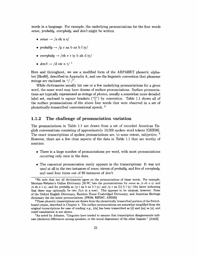


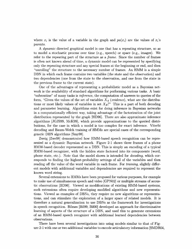


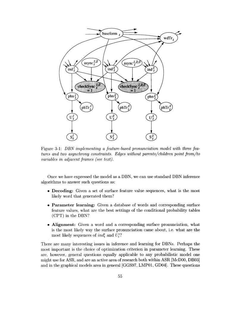


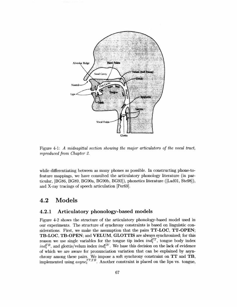


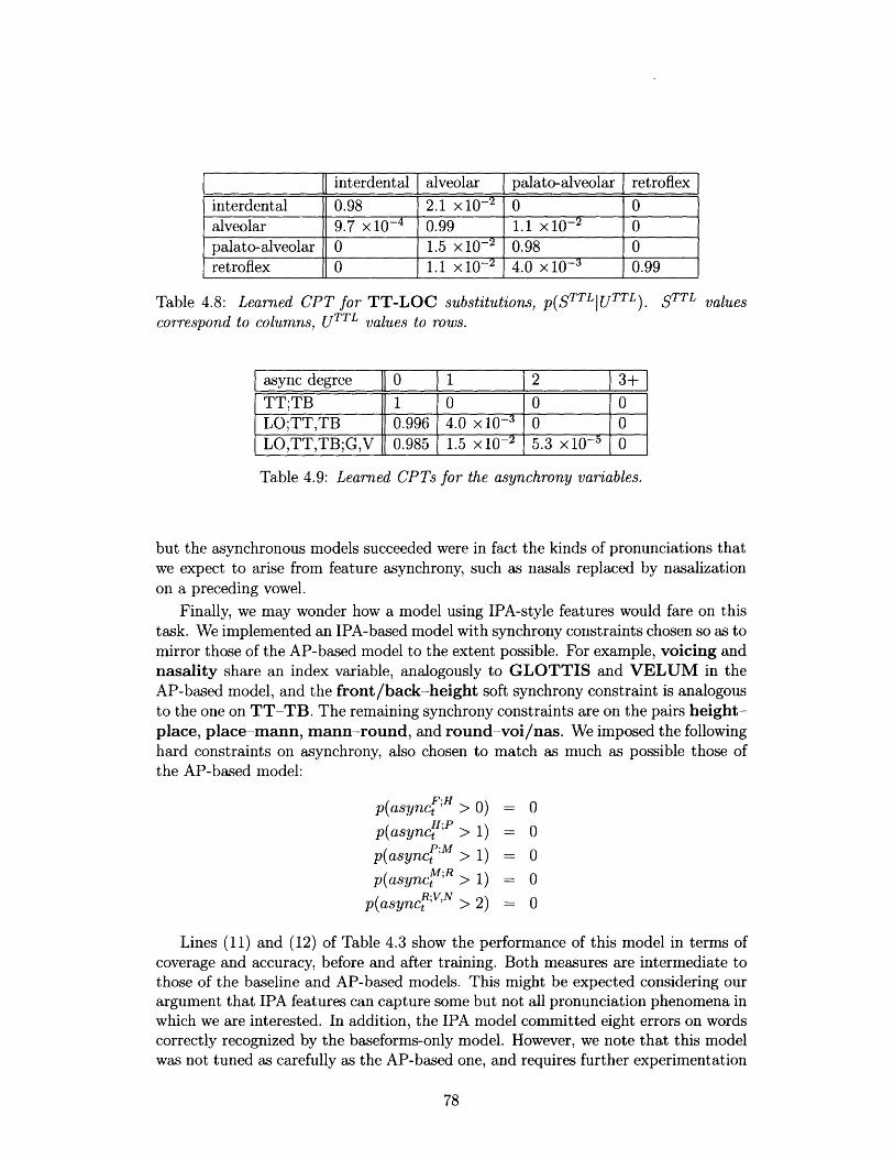


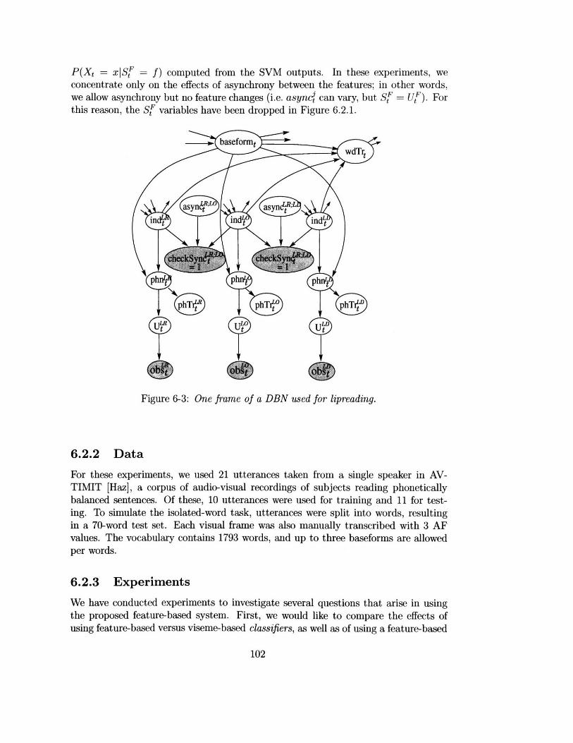

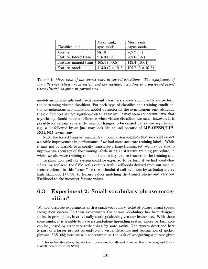


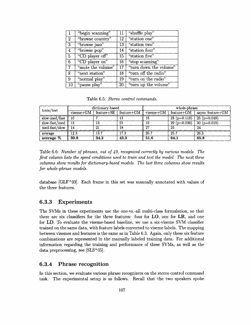


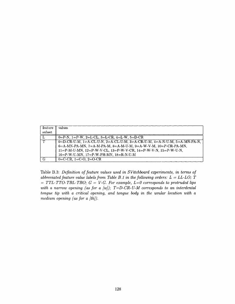


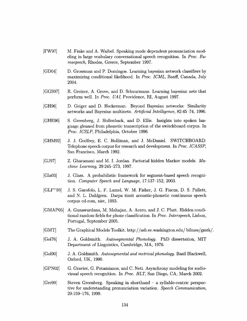


![Using Speech Recognition in Learning Primary School ... · 2.1. Windows Speech Recognition In general, a speech recognition process 14] consists of processing the speech which is](https://static.documents.pub/doc/80x56/603c385c36ee9629d81b13fc/using-speech-recognition-in-learning-primary-school-21-windows-speech-recognition.jpg)


