95 VOLUME V / INSTRUMENTS 2.5.1 Introduction A given amount of matter (usually called a system) can be characterized by uniform intensive properties in its whole volume or only in some of its parts; a portion of matter with uniform intensive properties is referred to as a phase. A heterogeneous system, therefore, consists of more than one phase: crossing the boundary separating two phases there is a sharp change in at least one intensive property (density, for example). Consequently single phase system and homogeneous system are, in this context, synonyms. Equilibrium conditions are particular conditions reached by a system fulfilling well-defined constraints (such as constant temperature and pressure) after some time (theoretically infinite) from which the system has no tendency to move. The state (defined as the ensemble of all the values of the thermodynamic variables of the system in a given condition; such thermodynamic variables are called state variables) of stable equilibrium is independent of time and previous system history, and it can resist minor fluctuations of its state variables. Such a definition distinguishes stable equilibrium conditions not only from every other non-equilibrium condition, whether stationary or not, but also from metastable equilibrium conditions. Systems in a state of equilibrium are much easier to describe than systems where transformations are being carried out. This a simplicity allows the equilibrium state to be described with a small number of state variables. These particular states (of equilibrium) are the field of application of the thermodynamic laws. These basic laws cannot be mathematically demonstrated; their validity relies on the absence of contrary experimental evidence. This chapter deals with equilibrium conditions in multi- phase multi-component systems without chemical transformations, meaning without any exchange of the atoms present in a system within the molecules of the various components. Since the fundamental work by Josiah Willard Gibbs at the end of the Nineteenth century (Gibbs, 1928) the theory which defines all the conditions for system equilibrium is well known. The main problem, which has not yet been completely resolved, for arriving at solutions in a numerical form suitable for practical applications is the representation of reality via models. In other words, the not yet satisfactory description of molecular interactions often does not allow the correct evaluation of the thermodynamic functions needed to characterize the equilibrium conditions of a real system. 2.5.2 General equilibrium conditions All systems, depending on the constraints they must fulfil, spontaneously proceed in a well-defined direction. It is common knowledge that the concept of entropy (a thermodynamic function which cannot be measured directly) must be introduced in order to take into account the direction in which real systems spontaneously proceed. Because entropy provides this information, it is also able to define the equilibrium state as that particular state from which the system has no tendency to spontaneously evolve. Entropy is an extensive state function defined in such a way that, following a spontaneous transformation in an isolated system, it can only increase. As a consequence, equilibrium conditions in an isolated system require entropy to assume the maximum value possible provided that all the constraints imposed by the system itself are fulfilled. Equilibrium states, as was mentioned earlier, can be defined by a small number of variables. In particular, it can be shown experimentally that the stable equilibrium extensive state (i.e. the value of all the extensive variables) of an isotropic single-phase multi-component system can be completely defined once the values of its internal energy U, volume V, and mole number n(n 1 , n 2 ,…) of each species are given. This is known as the first law of thermodynamics. Instead, the requirement of maximum entropy for equilibrium law of an isolated system is known as the second postulate of thermodynamics: there exists a function of the extensive variables of a system (U, V and n) called entropy, S, which is defined for all the equilibrium states and implies that the values of U, V and n, when no internal constraints are enforced in an isolated system, make the value of entropy maximum. As a consequence, when an isolated system is in equilibrium conditions the first differential of entropy must 2.5 Phase equilibria
Transcript
95VOLUME V / INSTRUMENTS
2.5.1 Introduction
A given amount of matter (usually called a system) can becharacterized by uniform intensive properties in its wholevolume or only in some of its parts; a portion of matter withuniform intensive properties is referred to as a phase. Aheterogeneous system, therefore, consists of more than onephase: crossing the boundary separating two phases there isa sharp change in at least one intensive property (density, forexample). Consequently single phase system andhomogeneous system are, in this context, synonyms.
Equilibrium conditions are particular conditions reachedby a system fulfilling well-defined constraints (such asconstant temperature and pressure) after some time(theoretically infinite) from which the system has notendency to move. The state (defined as the ensemble of allthe values of the thermodynamic variables of the system in agiven condition; such thermodynamic variables are calledstate variables) of stable equilibrium is independent of timeand previous system history, and it can resist minorfluctuations of its state variables. Such a definitiondistinguishes stable equilibrium conditions not only fromevery other non-equilibrium condition, whether stationary ornot, but also from metastable equilibrium conditions.
Systems in a state of equilibrium are much easier todescribe than systems where transformations are beingcarried out. This a simplicity allows the equilibrium state tobe described with a small number of state variables. Theseparticular states (of equilibrium) are the field of applicationof the thermodynamic laws. These basic laws cannot bemathematically demonstrated; their validity relies on theabsence of contrary experimental evidence.
This chapter deals with equilibrium conditions in multi-phase multi-component systems without chemicaltransformations, meaning without any exchange of the atomspresent in a system within the molecules of the variouscomponents.
Since the fundamental work by Josiah Willard Gibbs atthe end of the Nineteenth century (Gibbs, 1928) the theorywhich defines all the conditions for system equilibrium iswell known. The main problem, which has not yet beencompletely resolved, for arriving at solutions in a numericalform suitable for practical applications is the representation
of reality via models. In other words, the not yet satisfactorydescription of molecular interactions often does not allowthe correct evaluation of the thermodynamic functionsneeded to characterize the equilibrium conditions of a realsystem.
2.5.2 General equilibrium conditions
All systems, depending on the constraints they must fulfil,spontaneously proceed in a well-defined direction. It iscommon knowledge that the concept of entropy (athermodynamic function which cannot be measured directly)must be introduced in order to take into account the directionin which real systems spontaneously proceed. Becauseentropy provides this information, it is also able to define theequilibrium state as that particular state from which thesystem has no tendency to spontaneously evolve.
Entropy is an extensive state function defined in such away that, following a spontaneous transformation in anisolated system, it can only increase. As a consequence,equilibrium conditions in an isolated system require entropyto assume the maximum value possible provided that all theconstraints imposed by the system itself are fulfilled.
Equilibrium states, as was mentioned earlier, can bedefined by a small number of variables. In particular, itcan be shown experimentally that the stable equilibriumextensive state (i.e. the value of all the extensivevariables) of an isotropic single-phase multi-componentsystem can be completely defined once the values of itsinternal energy U, volume V, and mole numbern(n1,n2,…) of each species are given. This is known asthe first law of thermodynamics. Instead, therequirement of maximum entropy for equilibrium law ofan isolated system is known as the second postulate ofthermodynamics: there exists a function of the extensivevariables of a system (U, V and n) called entropy, S,which is defined for all the equilibrium states andimplies that the values of U, V and n, when no internalconstraints are enforced in an isolated system, make thevalue of entropy maximum.
As a consequence, when an isolated system is inequilibrium conditions the first differential of entropy must
2.5
Phase equilibria
be equal to zero. Since entropy is a state function, it has anexact differential and the following relation holds true:
[1]
A multi-phase system is constituted by manysingle-phase systems, for each of which all theaforementioned considerations must be fulfilled. Sinceentropy is an extensive variable, the system entropy can becalculated simply as the sum of the entropy of each phase.This can be put forward as the third law of thermodynamics: entropy is an extensive (in other words, theentropy of a system made up of several subsystems is givenby the sum of the entropies of the single subsystems),continuous and differentiable variable, which monotonicallyincreases with the internal energy. This allows the followingdefinitions:
[2]
[3]
[4]
As will be discussed below, T and P are the measurablevariables temperature and pressure, while mi is a chemicalpotential. The previous relation therefore becomes:
[5]
From this relation all the general equilibriumconditions among phases can easily be deduced. Allthermodynamic problems, including those of phaseequilibria, can be described by the general model of anisolated system represented by a container with rigid,adiabatic, impermeable walls divided by a wall into twosubsystems, A and B.
When the internal wall is impervious to matter (i.e. itdoes not allow mass exchange between the two subsystems),rigid (i.e. it does not allow work exchange between the twosubsystems), and non-adiabatic (i.e. it allows heat exchangebetween the two subsystems), both volume and mole numberof the two subsystems are constant and thereforedni
AdniBdVAdVB0. Moreover, as the whole system is
isolated the total internal energy is also constant; it followsthat the internal energy increase of a subsystem must beequal to the internal energy decrease of the other subsystem:dU AdU B. Since entropy is an extensive variable, usingthese relations it follows that:
[6]
which means that under equilibrium conditions necessarilyT AT B. Therefore, T has the physical meaning oftemperature and relation [6] requires the temperature of thesystems connected by a non-adiabatic boundary to be equalonce equilibrium conditions are attained. In other words, theequilibrium condition with respect to heat transfer is thattemperature is uniform, as experimentally verified.
Analogously, it is possible to deduce the equilibriumconditions with respect to work exchange. In this case theboundary separating the two subsystems is assumed to beimpervious to matter, but neither rigid nor adiabatic (thismeans that it allows heat and work exchange between thetwo subsystems). Along the same lines previously discussed,it can be demonstrated that: dni
AdniB0; dVA dVB;
dUAdUB. The maximum entropy requirement thusbecomes:
[7]
This relation implies that (seeing that TATB) PA mustbe equal to PB. Therefore, P has the physical meaning ofpressure and relation [7] requires the pressure of the systemsconnected by a non-rigid boundary to be equal onceequilibrium conditions are attained. In other words, theequilibrium condition with respect to work exchange is thatpressure is uniform, as experimentally verified.
Finally, equilibrium conditions with respect tomass transfer can be deduced. In this case theboundary separating the two subsystems is consideredto allow exchange of matter, heat and work. It isworthwhile noting that in this case the systems beingexamined can be thought of as two distinct phases inan isolated system. These different phases aresubsystems that can exchange mass and energy and soare separated by permeable, diathermal and mobilewalls. It follows that, analogously to what waspreviously discussed, dni
AdniB; dV AdV B;
dUAdUB and the equilibrium relation can be recastas the following:
[8]
+PAA
A
B
BA i
A
AiB
B iA
iTPT
dVT T
dn−
− −
=
µ µ
1
NN
∑ = 0
+ − = −
+=∑P
TdV
Tdn
T TdU
B
BB i
B
B iB
i
N
A BAµ
1
1 1
TdU P
TdV
TdnA
AA
AA i
A
A= + −1 µ
iiA
i
N
BB
TdU
=∑ + +
1
1
dS d S S dS dSA B A B= +( ) = + =
T TdU P
TPT
dA BA
A
A
B
B= −
+ −
1 1 VV A = 0
PT
dVT
dUA
AA
BB+ + +
1 PPT
dVB
BB =
dS d S S dS dST
dUA B A BA
A= +( ) = + = +1
TdU
T TB
B
A B+ = −
1 1 1
=dUA 0
dS d S S dS dST
dUA B A B
A
A= +( ) = + = +1
dSTdU
P
TdV
Tdni
ii
N
= + − ==∑1
01
µ
= −− ∂∂
∂∂
= −
≠
SU
Un TV i S V n
i
j i, , ,n
µ
∂∂
= → ∂
∂
=
≠ ≠
Un
Sni S V n
ii U V nj i j i, , , ,
µ
= − ∂∂
SU V ,, ,n n
∂∂
=UV
PTS
∂∂
= − → ∂∂
=UV
P SVS U, ,n n
∂∂
= → ∂∂
=US
T SU TV V, ,n n
1
Sni
+ ∂∂
=
≠=∑
U V ni
i
N
j i
dn, ,
01
dS SU
dU SV
dVV U
= ∂∂
+ ∂∂
+, ,n n
PHYSICAL AND CHEMICAL EQUILIBRIA
96 ENCYCLOPAEDIA OF HYDROCARBONS
This relation is fulfilled (TATB and PAPB beingin equilibrium conditions) when mi
AmiB. The variable
mi, whose physical meaning is less intuitive than that ofpressure and temperature, is usually referred to as thechemical potential. The chemical potential of the ith
species can be thought of as the internal energy changeinduced by adding to the system one mole of species iwhile keeping constant both the entropy and volume ofthe system, as well as the mole numbers of all the otherspecies.
Equation [8] requires, in equilibrium conditions, that thechemical potentials of each species in different subsystemsseparated by boundaries permeable to mass be equal. Sincethe previous equilibrium conditions with respect to heat andwork exchange require that also temperature and pressure bethe same, the general equilibrium condition between twomulti-component phases is:
[9]
where a and b represent two different phases, x being thecomposition and where a single value of both temperatureand pressure for both the phases has been explicitlyaccounted for. Note that the composition of the two phasescan be different. However, for single-component systems,meaning those containing only one pure species, thecomposition is constant and the previous relation becomes:
[10]
Relations [9] and [10] are, in practice, the first two stepsdescribed in the introduction for solving a problem usingthermodynamic tools. The problem of phase equilibria hasbeen expressed in the abstract terms of thermodynamics andthe solution has been found, represented by the equationswhich impose the equality of chemical potentials. Now theproblem is to bring these results ‘back to the real world’, inother words, to relate chemical potentials with thosemeasurable intensive variables of interest, such as pressure,temperature and the composition of the different phases.
It is useful to look at the problem first in terms ofdetermining the number of variables that need to be definedto identify the intensive state of a system, i.e. the value of allits intensive variables. In particular, the degree of freedom,or variance, of a system is the number of intensive variablesthat can be arbitrarily assigned.
Let us consider a system with F phases and Nspecies: the number of intensive variables required todefine the intensive state of each phase (temperature,pressure and composition) is equal to 2(N1)N1.Note that when composition is given as mole fractions, the number of mole fractions to be defined for each phase is equal to N1 since the Nth value can be calculatedusing the normalization relation: xN1i1
N1xi. Thenumber of intensive variables that must be given tocompletely characterize the intensive state of a systeminvolving F phases is therefore equal to F(N1).
The aforementioned equilibrium conditions requirethe temperature and pressure of each phase to be equal;the chemical potential of each species in the differentphases must be equal as well. Since chemical potential,which is an internal energy derivative, depends on theintensive variables of the system (temperature, pressureand composition), the relations linking these intensivevariables are the following:
[11]
Generally there are (F1)(F1)N(F1)(N2)(F1) equations involving F(N1) variables.In order for the system of equations to have a single root,in other words the number of independent equations mustbe equal to the number of variables, it is necessary todefine the values of F(N1)(N2)(F1)NF2variables, which is equal to the degree of freedom, ,of the system:
[12] N F 2
For instance, when a system involves two phases and twospecies it is necessary to give the values of 2 intensivevariables. When NF1, the previous relation gives 2which is the well-known experimental finding stating thatthe intensive state of a single-component single-phasesystem is completely defined once the values of twointensive variables are given.
Once the values of intensive variables are given, thevalues of all the other intensive variables can be calculatedthrough the assigned variables and the aforementionedequilibrium relations. How to use these relations, withparticular reference to the chemical potential equality, tocompute the values of the equilibrium intensive variablesvalues for a system involving F phases and N species will beexamined later. It is useful, however, to start with a briefdescription of the equilibrium conditions for closed systemssubject to conditions other than maintaining volume andinternal energy constant.
The first and second law of thermodynamics takentogether can provide the following general relation (here Vmeans volume) which is valid for spontaneoustransformations in closed systems:
[13]
For a system where volume and internal energy areconstant (i.e. an isolated system) dUdV0 and theprevious relation leads to:
[14]
which means that entropy can only increase and therefore, inequilibrium conditions, it must be maximum following thesecond law of thermodynamics. For a system where volumeand entropy are constant, dSdV0 and relation [13]becomes:
[15]
which means that internal energy can only decrease and,therefore, in equilibrium conditions, it must be minimum.For a system where volume and temperature are constant,dTdV0 and relation [13] becomes:
[16]
which means that Helmholtz free energy, A, can onlydecrease and, therefore, in equilibrium conditions, it must beminimum. Finally, for a system where pressure and
TdS dU PdV d TS dU d TS U dAT V
− − = ( )− = −( )=− ≥,
0
dUS V,
≤ 0
dSU V,
≥ 0
TdS dU PdV− − ≥ 0
T T FP P F
F
F
1
1
1
1
= = −= = −
...
...
relations
relations
µ11
1
1
1
1
= =
= =
−( )...
...
...
µ
µ µ
F
N NF
N F relationns
µ µα βi iT P T P( , ) ( , )=
µ µα α β βi iT P T P( , , ) ( , , )x x=
PHASE EQUILIBRIA
97VOLUME V / INSTRUMENTS
temperature are constant, dTdP0 and relation [13]becomes:[17]
which means that Gibbs free energy, G, can only decreaseand, therefore, in equilibrium conditions, it must beminimum.
2.5.3 Equilibrium betweensingle-component phases
A solid at a given temperature and pressure when heated atconstant pressure usually changes its temperature andmolar volume as shown in Fig. 1. At the beginning the solidis represented by point 1. When heated, its temperature andmolar volume increase until point 2, where it starts to melt:here a phase transition proceeds with the presence of both asolid and a liquid phase in equilibrium conditions. Thesolid phase molar volume is equal to v2
S, while the molarvolume of the liquid phase which is formed from meltingthe solid is equal to v3
L. Since the two phases are inequilibrium conditions, their temperatures must be equaland consequently the tie line connecting points 2 and 3 inequilibrium conditions is horizontal (all thesingle-component phase transitions proceed at constanttemperature and pressure). This also implies that at a givenpressure value, melting (or fusion) temperature of a purespecies (point 2) is equal to the freezing (or solidification)temperature (point 3): at a given pressure value there existsonly one temperature value where liquid and solid phasescan coexist, called melting or freezing temperature.Obviously, at a given temperature value, there exists onlyone pressure value where liquid and solid phases cancoexist, called melting or freezing pressure. This is evidentif one remembers that the degree of freedom of asingle-component system is equal to 3F; when twophases are involved the degree of freedom is equal to one:given the value of an intensive variable, for instancepressure, the values of all the other intensive variables,including temperature, are fixed.
When the partially melted species is heated further, theamount of liquid increases, as does the molar volume of thetwo-phase mixture (that is, the volume occupied by one moleof the species, partially solid and partially liquid) becausethe liquid molar volume is usually larger that that of thesolid. The molar volume of the two-phase mixture is inbetween the values of the liquid and solid molar volume inequilibrium conditions (points 2 and 3) and it isconsequently represented by a point on line 23. This valuecan be calculated from a weighted average (based on themole numbers) of the molar volumes values of the solid andliquid: (nLnS)vnLv3
LnSv2S. From this relation the molar
volume of a two-phase mixture can be expressed as afunction of the proportion of liquid in the mixture,xnL(nLnS):
[18]
This relation is fully general and permits the calculationof the value of a generic molar variable of a two-phasemixture, m, as mxmL(1x)mS.
The amount of heat required to completely melt onemole of compound is called molar latent heat of melting.Since this heat is exchanged at constant pressure, it is alsocalled molar melting enthalpy. The molar latent heat offreezing (or molar freezing enthalpy) is equal to the meltingvalue disregarding the sign, since in this case heat isremoved from, not added to, the system.
When all the matter is melted (point 3) the heat put intothe system increases the temperature and the molar volumeuntil point 4, and the species begins to boil. At this pointliquid and vapour in equilibrium conditions aresimultaneously present. The molar volume of the vapourphase is equal to v5
V, while that of the liquid phase is equal tov4
L. Since the two phases are in equilibrium they are at thesame temperature and therefore the tie line connecting point4 to point 5 is horizontal. As in the previous case ofliquid-solid equilibrium, at a given pressure value the boilingtemperature of a pure species (point 4) and its dew point(point 5) are equal. At a given pressure value there existsonly one temperature value where liquid and vapour inequilibrium conditions can exist, called boiling or dewtemperature. Obviously, at a given temperature value thereexists only one pressure value where liquid and vapour inequilibrium conditions can exist, called vapour pressure.
As in the solid-liquid phase transition, continuing to heatthe system leads to an increase in the amount of vapour, andconsequently the molar volume of the two-phase mixtureincreases since the molar volume of the vapour is larger thanthe molar volume of the liquid. The molar volume value of thetwo-phase mixture is in between the values of the liquid andvapour phases (points 4 and 5); it corresponds to one point onthe line 4-5 and can be calculated with a relation analogous to the one seen earlier as: vxv5
V(1x)v4L where xnV(nLnV)
is the vapour quality of the two-phase mixture. This relation isalso fully general and the value of any molar quantity of themixture, m, can be calculated as mxmV(1x)mL.
The amount of heat required to completely vaporize onemole of compound is called molar latent heat (or enthalpy)of vaporization, which corresponds (disregarding the sign) tothe molar latent heat (or enthalpy) of condensation. Heatingthe system further, its temperature and molar volumeincrease to point 6.
v nn n
v nn n
v xv x vL
L SL
S
L SS L S=
++
+= + −( )3 2 3 2
1
,
= − −( ) = − ≥d TS U PV dGT P
0
TdS dU PdV d TS dU d PV− − = ( ) − − ( ) =
PHYSICAL AND CHEMICAL EQUILIBRIA
98 ENCYCLOPAEDIA OF HYDROCARBONS
tem
pera
ture TbTd
TmTs
molar volume
solid
liquid
1
23
45
6
vapour
v2S v3
L v4L vV
5
Fig. 1. Trends of temperature and molar volume during heating of a pure species at constant pressure.
The same information can be summarized in a P-Tdiagram, as shown in Fig. 2. The three lines represent theboundaries of the regions where different phases exist(namely: solid, liquid and vapour): crossing each of theseboundaries indicates a phase transition. For instance, thevaporization boundary identifies the region where onlyvapour exists at a given value of temperature, T1, as theregion with pressure values lower than P°(T1), which is thevapour pressure at temperature equal to T1 for the consideredspecies. For pressure values larger than P°(T1) only the liquidphase can exist. Only when the pressure value is equal toP°(T1) can vapour and liquid phases exist simultaneously inequilibrium conditions. Similar conclusions can be derivedfrom the sublimation line (vapour-solid equilibrium) andfrom the melting line (liquid-solid equilibrium). Above thecritical temperature no phase transition can exist and theequilibrium line vanishes. In Fig. 2 the triple point is alsoidentified as the only point where three phases can existsimultaneously in equilibrium conditions. This point isunique (i.e. the pressure and temperature are fixed) in thatwhen the number of phases is equal to three the degrees offreedom is equal to zero and no intensive variables can bearbitrarily chosen.
Given that in equilibrium conditions two phases a and bmust necessarily have the same temperature and pressure,the equilibrium conditions for mass transport between thephases means that:
[19]
where P° is the unique value of pressure at which the twophases of the species in question can be present inequilibrium when the system temperature is equal to thegiven value.
It is known that the chemical potential is directly relatedto the Gibbs free energy, through the following differentialequation:
[20]
showing that the chemical potential is equal to the partialmolar Gibbs free energy.
Partial molar properties represent the change of ageneric mixture property M due to the addition of one moleof species i while keeping temperature, pressure and molenumber values of all the other species constant:Mi(Mni)T,P,nji
. An alternative meaning of partial molarproperties is the molar value of the property when thespecies is in a mixture. Consequently, all the mixtureproperties can be calculated through the values of the partialmolar properties and the mixture composition asM(T,P,n)N
i1M
i(T,P,x)ni or, in molar terms, asm(T,P,x)N
i1M
i(T,P,x)xi.Since for a pure species the partial molar Gibbs free
energy is equal to the molar Gibbs free energy, the chemicalpotential and the Gibbs free energy are related to each otherthrough the following relations:
[21]
The general equilibrium relation [19] for asingle-component system becomes, considering for the sakeof example the vapour-liquid equilibrium:
[22]
A system involving a liquid and a vapour phase inequilibrium conditions at temperature T1 and pressure P°(T1)is represented by point 1 in Fig. 2. When the systemtemperature increases by a small amount dT, the vapourpressure must also increase by a small amount dP in orderthat the two phases continue to exist in equilibriumconditions. The system evolves towards point 2 in Fig. 2.Both for the conditions of point 1 and of point 2 theequilibrium relation must be fulfilled:
[23]
Since for both the phases g[T1dT, P1°(T1)dP]g[T1, P°1(T1)]dg, it follows that dgLdgV. Using the molarGibbs free energy differential for a pure species:
[24]
an equation relating the vapour pressure to the temperaturethrough latent evaporation heat (∆hevhVhL) and the molarvolume change in the phase transition (∆vevvVvL), whichis known as the Clapeyron equation, can be deduced:
[25]
Similar equations can be deduced for all the other phasetransitions, that is, liquid-solid and vapour-solid, using theheat and molar volume changes corresponding to theconsidered phase transition.
Since the heat of evaporation, melting and sublimationare always positive, the slope (dP/dT ) of the equilibriumlines in Fig. 2 depends on the sign of ∆v. The molar volume
dP
dT
s s
v v
h h T
v v
h
T v
V L
V L
V L
V L
ev
ev
°=
−
−=
−( )−
=∆
∆
dg s dT v dP dg s dT v dPL L L V V V= − + = = − +
g T dT P TL1 1
,+ °(( )+ = + °( )+ dP g T dT P T dPV1 1
,
g T P T g T P TL V1 1 1 1, ,°( ) = °( )
g T P g T PL V, ,° °( ) = ( )
µ T( ,PP g T P) ( , ) ( )= purespecies
µii T P n
iT P Gn
G T Pj i
( , , ) ( , , )
, ,
x x=∂∂
=
≠
dG VdP SdT dni ii
N
= − +=∑µ
1
µ µα βT P T P, ,° °( ) = ( )
PHASE EQUILIBRIA
99VOLUME V / INSTRUMENTS
pres
sure
T1
P°(T1)dP
T1dT
dP
dT
P°(T1)
temperature
solid
liquid
melting line for species that reducetheir volume when melting
melting line for species thatincrease their volume when melting
critical point
triple point
evaporationline
sublimationline
vapour
1
2
Fig. 2. Phase diagram for a pure species.
change from liquid to vapour and from solid to vapour isalways positive and consequently the slope of theevaporation and sublimation lines is always positive. In otherwords, the vapour pressure of liquids and solids alwaysincreases with temperature. For many species ∆vfus0, thatis, the liquid molar volume is larger than the correspondingsolid molar volume in equilibrium. For these species dP/dTis positive also for the liquid-solid equilibrium boundary andthe melting temperature increases with pressure. However,for other species such as water, whose liquid molar volumeis smaller than the corresponding solid molar volume, theslope of the melting equilibrium line is negative and themelting temperature decreases as pressure increases.
For an evaporation curve when pressure values areneither too high nor too close to the critical point, theprevious relation can be approximated considering thevapour molar volume to be much greater than the liquidmolar volume and similar to that of an ideal gas,∆vevvVvLvVRTP, which provides to theClausius-Clapeyron equation:
[26]
This equation can be used to estimate the latentevaporation heat through two values of the vapour pressure,or to deduce the trend of the vapour pressure with respect totemperature. Neglecting the dependence of the evaporationheat on the temperature, a reasonable approximation in asmall temperature range, the previous relation can be recastas:
[27]
showing that the logarithm of the vapour pressure is linearlyrelated to the inverse of the temperature.
2.5.4 Equilibrium between multi-component phases
Having established that temperature and pressure in allequilibrium phases must be equal also for mixtures, to showmass transfer equilibrium conditions among the phases it isnecessary to relate the chemical potential of a species in amixture to measurable properties. Following the approachproposed by Gilbert Newton Lewis, fugacity, fi, is definedthrough the differential relation:
[28]
Since, as will be discussed below, for a mixture of idealgases the chemical potential is related to the partial pressureas:
[29]
and remembering that all fluids at sufficiently low pressurevalues behave like ideal gases, the previous fugacitydefinition is complemented by the following:
[30]
From these relations it is clear that the fugacity of anideal gas is equal to the partial pressure (or the total pressurefor a pure species). Considering a system containing twophases in equilibrium, defined as a and b, the previousrelation can be integrated between the conditions of the twophases in equilibrium:
[31]
Since in equilibrium conditions the chemical potentialsof each species in the two phases must be equal, this relationleads to the following condition for phase equilibrium,absolutely equivalent to the equality of chemical potential:
[32]
In order for a system to be in equilibrium with respect tomass transfer, the fugacity of each species must be the samein all the phases.
For a system involving N species and two phases, theintensive variables required to fully characterize the systemare temperature and pressure (two variables since we knowthat temperature and pressure of both the phases must beequal) and the mole fractions in each phase (N1 variablesfor each phase, since the Nth mole fraction can be calculatedfrom the other N1 mole fraction as a complement to one).The total number of intensive variables is therefore equal to2N. The degrees of freedom for this system is equal toN22N, and consequently N intensive variablesmust be given in order to compute the other N intensivevariables. The N equations required to compute the Nunknowns are relations [32], one for each species present inboth the phases. These equations are complemented by thetwo stoichiometric equations to compute the Nth molefraction in both the phases:
[33]
All the particular cases that will be discussed belowrequire the solution of the set of algebraic equations [32] and[33]. Obviously, the first problem to be faced refers to thecorrelation of fugacity to measurable properties, whichmeans that the solution of the problem is in trying to bringthe abstract language of thermodynamics down to the realworld.
Fugacity from equations of state: direct methodsDirect methods use as a reference an ideal gas mixture,
that is, a mixture without interactions between moleculeswhose behaviour is represented by the equation of statePvRT and by the Gibbs theorem (all the partial molarproperties, except for volume, of a species in an ideal gasmixture are equal to the corresponding molar properties of
x
x
ii
N
ii
N
α
β
=
=
∑
∑
=
=
1
1
1
1
ˆ ( , , ) ˆ ( , , )f T P f T Pi iα α β βx x=
x xx
µ µα α β βα α
− =i iiT P T P RTf T P
( , , ) ( , , ) lnˆ ( , , ))
ˆ ( , , )f T Piβ βx
d RT d fiT P
T P
iT P
T P
µα
β
α
β
α
β
α, , ,
, , ,
, , ,
, , ,
ln ˆ
x
x
x∫ =
xxβ
∫
P→
=0
limfP
i
i
1
d RTd Pi T iµ , ln=
d RTd fi T iµ , ln ˆ=
lnh
Rev→ =∆
PP T P T
T T
° °2 1
1 21 1
( ) ( ) −( )
lnP TP T
hR T T
ev°
°2
1 1 2
1 1( )( ) = −
→
∆
dPdT
P hRT
d PdT
hRT
ev ev° =°
→ ° =∆ ∆
2 2
ln
PHYSICAL AND CHEMICAL EQUILIBRIA
100 ENCYCLOPAEDIA OF HYDROCARBONS
the pure species at the mixture temperature but at a pressureequal to the partial pressure of the considered species in themixture): Mi
*(T,P,x)mi*(T,Pi), where M is a generic
thermodynamic property.The Gibbs theorem allows the calculation of all the
partial molar properties of an ideal gas mixture from themolar properties of the pure species, apart from the partialmolar volume which obviously is calculated Vi
*(T,P,x)(V *ni )T,P,nij
RTPvi*(T,P).
Using the Gibbs theorem it can be easily demonstratedthat there is a simple relation [29] between chemicalpotential and partial pressure for one component of amixture of ideal gases:
[34]
This equation for a pure species becomes:
[35]
So called direct methods, since they use as a referencean ideal gas mixture, introduce the fugacity coefficient /i, avariable that takes into account the departure of the systembehaviour from that of an ideal gas. This coefficient isdefined as the ratio of the fugacity of a species in a mixtureto the fugacity of the same species in an ideal gas mixtureunder the same conditions:
[36]
It is clear that the fugacity coefficient of a species in anideal gas mixture is equal to 1, while for a pure specie thefugacity coefficient becomes:
[37]
As a consequence, the problem of phase equilibriumcharacterization has been traced to the calculation ofchemical potentials to the fugacities and now finally to thefugacity coefficients. Direct methods deal with this lastproblem by relating the fugacity coefficients to the Gibbsfree energy. The calculation of the Gibbs free energy usingdirect methods is based on the calculation of the departure ofthe thermodynamic function of a real fluid, G, from that ofan ideal gas, G*, called departure function: GRGG*.Since the thermodynamic properties of an ideal gas can becalculated exactly, knowing either the Gibbs free energy orthe departure Gibbs free energy provides the sameinformation.
The dimensionless form of the departure molar Gibbsfree energy, gRRT, can be easily calculated from thefollowing differential relation:
[38]
where the relations dgvdPsdT and ghTs have beenused.
As usual, in thermodynamics the value of a statefunction is calculated following the easiest thermodynamicpattern. In this case, the value of gRRT can be easilycalculated through an isothermal path:
[39]
The zero value of the lower integration limit arises fromthe fact that all the fluids behave like an ideal gas when thepressure approaches zero, and consequently when thepressure approaches zero all the departure functions areequal to zero. The previous relation, introducing thedefinition of the compressibility factor ZPv/RT, leads tothe following equation:
[40]
The important implication of this equation is that, basedon a given Equation Of State (EOS), that is, the relationZ(T,P,x), deduced from experimental measurements P-v-T-x, the departure molar Gibbs free energy can becalculated, and thus the value of the Gibbs free energy. Thisplays a special role in the thermodynamics of mixtures, as itis possible to demonstrate that all the other variables inquestion can be derived from it: Gibbs free energy can beconsidered the foundation function of all thermodynamicproperties. This means that by using an EOS it is possible tocalculate all thermodynamic functions, confirming the greatimportance of EOS in thermodynamics.
For a real fluid the fugacity coefficient, /i, can be relatedto the departure partial molar Gibbs free energy andconsequently calculated through an EOS. Integrating thefugacity from an ideal gas state to a real fluid state itfollows:
[41]
Since the chemical potential of a species in a mixture isequal to the partial molar Gibbs free energy and introducingthe definition of departure function, the previous relationcan be recast in the following manner:
[42]
As a consequence, the fugacity coefficient of a speciesin a mixture can be calculated from the departure Gibbs freeenergy as:
[43]
P
i
n Z dPP
n=
∂ −( )
∂
∫ 10
=
≠T P nj i, ,
,
( , , )R
iT P
ng T P RT
n=
∂ ∂
x
,,nj i≠
=
ln ˆ ( , , )( , , )
φi
R
iT
T PG T P RT
nx
x=
∂ ∂
,, ,P nj i≠
=
RT Tiln ˆ ( ,= φ PP, )x
G T P G T P G T Pi i iR( , , ) ( , , ) ( , , )*x x x− = =
Tiµ ( ,PP T P RTfP
RTii
ii, ) ( , , ) ln
ˆln ˆ*x x− = =µ φ
d RT d fiT P
T P
iT P
T P
µ, , ,*
, ,
, , ,*
, ,
ln ˆ
x
x
x
x
∫ ∫=
Pv
RT= −
1ddP
PZ
dP
P
P P
0 0
1∫ ∫= −( )
g T P
RT
v v
RTdP
R P, *( )− =
−
=∫0
0
dg
RT
v
RTdP T
Rg P RT RPR
=
=∫ ∫
0 0
( )/
consttant
v
RTdP
h
RTdT
v
RTdP
h
RTdT
R R
2 2− −
= −
* *
dg
RTd
g
RTd
g
RT
v
RTdP
h
R
R
=
−
= −
*
TTdT
2−
φ T Pf T P
f T P
f T P
P,
,
,
,*
( ) = ( )( )
=( )
ˆ , ,ˆ , ,
ˆ , ,
ˆ , ,
*φi
i
i
iT Pf T P
f T P
f T Px
x
x
x( ) = ( )( ) =
( )PPxi
d T P RTd Pµ*( , ) ln=
d T P RTd Pi iµ*( , , ) lnx =
PHASE EQUILIBRIA
101VOLUME V / INSTRUMENTS
It should be noted that the dependence of Z on ni derivesfrom the mixing rules used in the EOS. For a pure species,the compressibility factor does not depend on composition;therefore, the previous relation becomes:
[44]
If an EOS is known, the integrals involved in theserelations can be calculated analytically (in the case of amixture, preceded by the derivative) and then computing thefugacity coefficient value.
One of the simplest EOS is that of the correspondingstates. This EOS states that the compressibility factor of allthe fluids depends only on the reduced temperature and thereduced pressure (which are defined as the ratio oftemperature or pressure and the related critical value:TRTTC and PRPPC); this means that ZZ0(TR,PR). Thisrelation in practice states that two fluids that are in twocorresponding states (i.e. characterized by the same reducedtemperature and reduced pressure) have the samecompressibility coefficient.
A large amount of work has been undertaken devoted toobtaining general correlations of the compressibility factoras a function of the reduced variables that are able tocorrectly reproduce the experimental results. The complexityof these correlations makes it more useful to provide theinformation in tables or graphs, such as the well-knowntables by B. I. Lee e M. G. Kesler (1975).
Apart from the region close to the saturation boundary orto the critical point, this EOS foresees the compressibilityfactor of low-polar species within 5%. On the other hand, forlarge-polar species or quantum gases (hydrogen, helium andneon) large differences with the experimental values of thecompressibility factor can be found. To increase theagreement with the experimental findings a third parameteris often introduced in the corresponding state equation, thePitzer acentric factor w:
[45]
In this relation (usually referred to as the generalizedcorresponding state equation) the value of Z1 (which is alsoavailable in a graph or a table as a function of the reducedvariables) is usually a small correction to the Z0 value, andconsequently it can often be ignored in a first analysis.
Fig. 3. Generalized diagramof fugacity coefficient as a function of reducedvariables (Sandler, 1989).
Using this EOS also allows the fugacity coefficientrelation for pure species to be generalized as:
[46]
It should be noted that the fugacity coefficient dependsonly on the reduced pressure and on the compressibilityfactor. Introducing the generalized corresponding stateequation it follows:
[47]
Both the integrals depend only on TR and PR, as well ason Z0(TR,PR) and Z1(TR,PR). It follows that the two termsln(/)0 and ln(/)1 depend only on the reduced variables andthey can be given in tabular or graphical form in the sameway as for the two functions Z0(TR,PR) and Z1(TR,PR).Analogously to the case of the compressibility factor, thefunction ln(/)1 represents a correction to the values of /0
and consequently it can often be ignored at first. The valuesof /0 as a function of the reduced temperature and reducedpressure, both for liquid phase and vapour phase, aresummarized in the graph in Fig. 3. Diagrams like this permita quick evaluation of the departure behaviour of a given fluidcompared to an ideal gas at given temperature and pressurevalues.
An important difference between pure fluids andmixtures is, in the case of mixtures, that Z does not dependonly on the reduced variables but also on the composition.This means that for mixtures, but not for pure fluids, it is notpossible to derive generalized correlations for computing thefugacity coefficients valid for any mixture as a function ofonly the reduced variables.
For pressure values that are not excessively high (lowerthan 15 bar) and for the gas phase, virial EOS truncated atthe second coefficient B, Z1BPRT, gives reasonablepredictions of the compressibility factor. Using this EOS thefollowing relation for the fugacity coefficient can bededuced:
[48]
Virial EOS can represent only the gas phase behaviour.When the liquid phase is involved, more complex EOS arerequired, such as cubic equations. The general equationrepresenting a cubic EOS for volume (or for thecompressibility factor) is the following:
[49]
where
[50]
The value or meaning of the symbols in these equations forsome common cubic EOS is summarized in Table 1. The previousrelation can be recast in terms of compressibility factor as:
[51]
The coefficients of this equation for some commoncubic EOS are also summarized in Table 1. Since cubic EOSgive the compressibility factor not as an explicit function ofpressure, but as an explicit function of volume, a change ofvariables is required in the integral in equation [44] in orderto compute, inserting relation [49], the fugacity coefficientwhich takes the general form:
[52]
Through the parameters e and s, given in Table 1 for thevarious cubic EOS, different operative relations forcomputing the fugacity coefficient values of both liquids andvapours can be deduced.
ln ln( )
( )lnφ
ε σσε
= − − − +−
++
Z v b Zv
abRT
v bv b
1
Z Z Z3 2 0+ + + =β γ δ
a TT RT
Pb
RTP
a c
c
b c
c
( )( , )
=( )
=Ω Ωα ω
2
Pv
RT
v
v b
a T v
RT v b v b=
−−
+( ) +( )( )
ε σ
lnφ = −( ) = + −
=∫ ∫Z
dP
P
BP
RT
dP
P
BP
RT
P P1 1 1
0 0
ω+ Z11
0
0 1dPP
TR
R
PR
∫ = ( ) + ( ) =ln lnφ ω φ constant
lnφ ω= + −( ) = −( ) +∫ ∫Z ZdPP
ZdPP
R
R
PR
R
PR R0 1
0
0
0
1 1
, ,ω= ( )− Z T Pd
R R 1PPP
TR
R
PR
=∫ constant0
lnφ = −( ) =∫ Z dPP
P
10
PHASE EQUILIBRIA
103VOLUME V / INSTRUMENTS
Table 1. Values or meaning of some symbols found in the general cubic EOS form for van der Waals (vdW),Redlich-Kwong (RK), Redlich-Kwong-Soave (RKS) and Peng-Robinson (PR). For all EOS AaP/(RT )2
except RK where AaP/[(RT)2T1/2] and BbP/(RT )
vdW RK RKS PR
a(T,w) 1 TR0.5 [1(0.4801.574w0.176w2)
(1TR0.5)]2
[1(0.374641.54266w0.26992w2(1TR
0.5)]2
e 0 0 0 0.414214
s 0 1 1 2.414214
Wa 27/64 0.42748 0.42748 0.457235
Wb 1/8 0.08664 0.08664 0.077796
b 1B 1 1 1B
g A ABB2 ABB2 A2B3B2
d AB AB AB ABB2B3
Given temperature and pressure values, the parameters inequations [51] and [52] can be calculated for a given EOS.Solving cubic equation [51] three roots are always found, butthe only roots with a physical meaning are the real andpositive roots. When more than one real positive root isfound, the larger value is retained when the pressure is lowerthan the vapour pressure at that temperature and so only thevapour phase is present, while the lower value is retainedwhen the pressure is larger than the vapour pressure at thattemperature and so only the liquid phase is present. Whenthe pressure is equal to the vapour pressure at the giventemperature both the phases exist in equilibrium conditionsand both the larger and the lower values must be retained.The central value does not represent a stable equilibriumstate and therefore it is never retained. Once the value of thecompressibility factor, Z, is calculated, the value of the molarvolume can be compute too, vZRTP, as well as the valueof the fugacity coefficient though equation [52].
In the case of mixtures, the same EOS can be usedprovided that the energetic and geometric parameter valuesused with these EOS refer to the given mixtures. Theseparameters can be calculated based on the parameter valuesfor pure species as well as on the mixture composition usingsuitable ‘mixing rules’ (which give the dependence on thecomposition) and ‘combination rules’ (which give thedependence on the pure-species parameters). Compositiondependence of the compressibility factor, which is requiredto compute the derivative in equation [43], is thereforeconfined to the mixing rules considered.
For the virial EOS truncated at the second term, themixing rule that gives the mixture coefficient:
[53]
In this relation the parameters characterized by thesame double subscript, Bii, are the second coefficients ofthe virial of the pure species and so account for two-bodyinteractions between like molecules. The parameterscharacterized by different subscripts, Bij, account for two-body interactions between different molecules. Since theseparameters account only for two-body interactions, theirvalues can be derived from experiments involving purespecies or, at most, mixtures of two components. Thebehaviour of mixtures with more than two componentscan be foreseen using only these parameters. Introducingthis mixing rule in general equation [43], the followingequation for computing the fugacity coefficient of aspecies in a mixture can be derived:
[54]
As previously seen for pure species, using cubic EOS itis possible to obtain the following general relation forcomputing the fugacity coefficient of a species in a mixture:
[55]
where the dependence on the composition is confined in thevalue of the derivatives with respect to the mole number ofthe ith species of both the geometric and energetic mixture
parameters, which in turn depend only on the particularmixing rule considered:
[56]
Usually, for cubic EOS quadratic (or van der Waals)mixing rules are used for any parameter p (which cancorrespond both to a and b); these mixing rules are equal tothe aforementioned mixing rule for the virial EOS:
[57]
Also in this case the parameters characterized by thesame double subscript account for two-body interactionsbetween like molecules, while the parameters characterizedby different subscripts account for two-body interactionsbetween different molecules. Assuming as a combinationrule a simple mean, pij(pipj)2, the quadratic mixing rulesimplifies to a linear mixing rule:
[58]
which is normally used for the geometric parameter b. Whenusing as a combination rule a geometric mean, pij
123
pi pj, thequadratic mixing rule reduces to:
[59]
which is normally used for the energetic parameter a. Thechoice of a geometric mean for the energetic parameterarises from the analogy with the rule used for computing theintramolecular potential between different molecules whenLondon dispersion forces prevail. As a consequence, thismixing rule is expected to perform correctly for mixtureswhen the London dispersion forces prevail. Using thequadratic mixing rule, explicit relations for the derivativesinvolved in the general relation for the fugacity coefficientscan be obtained:
[60]
from which the special cases arising from the two combination rules usually used for parameters a e b can be deduced:
[61]
Using the various EOS summarized in Table 1 severalrelations for computing the fugacity coefficient of a speciesin a mixture can be deduced. Quadratic mixing rules cannotcorrectly reproduce mixtures with strong intramolecularinteractions. Moreover, since EOS arise from the ideal gasequation of state, their predictions are more accurate for thegas phase than for the liquid phase.
Among the many alternative mixing rules proposed toremedy this problem, the Wong-Sandler rules areparticularly effective. These mixing rules try to make theEOS reproduce reliable results both in the region at highdensity (the liquid phase) and in the region at low density(the vapour phase). To achieve these results these mixingrules are derived requiring on the one hand that the EOS be
b b
a a a ai i
i i
=
= − + 2
pnp
np pi
i T n
jij
N
j i
=∂( )∂
= − +
≠
=∑,
21
p x pi ii
N= ( )=∑ 1
2
p x pi ii
N T= ==∑ 1
x p
p x x pi j ijj
N
i
N T= === ∑∑ 11
x xp
anan
bnbn
ii T n
ii T n
j i
j i
=∂( )∂
=∂( )∂
≠
≠
,
,
ε σa
bRT+
−( ) 1++ −
++
aa
bb
v bv b
i i lnσε
ln ˆ ( , , ) lnφiiT P
bb
Zv b Z
vx = −( ) − −( )
+1
ln ˆ ( , , )φi jij
NT P B B PRT
x = −( )=∑2 1
B x x Bi j ijj
N
i
N=
== ∑∑ 11
PHYSICAL AND CHEMICAL EQUILIBRIA
104 ENCYCLOPAEDIA OF HYDROCARBONS
able to reproduce correctly the excess Helmholtz free energyof the mixture (excess functions will be discussedextensively later; here it is sufficient to note that excessfunctions account for the departure of the behaviour of amixture, usually a liquid, from that of an ideal mixture wherethe intramolecular interactions between like and differentmolecules are the same) at infinite pressure, that is, in theregion at high density. This is carried out using theexperimental information available in terms of excess Gibbsfree energy, gE, at medium-low pressure. On the other hand,the mixing rules must also give the correct quadraticdependence of the second virial coefficient from thecomposition. This means that the EOS will perform correctlyalso where the virial EOS performs well, that is, in thelow-pressure region. The mixing rules arising from theseconstraints are the following:
[62]
where C is a parameter whose value depends on theparticular EOS considered. When using RKS(Redlich-Kwong-Soave) EOS the C parameter is equal to0.69315, while when using PR (Peng-Robinson) EOS it isequal to 0.62323. From these mixing rules, explicit relationsfor the derivatives in the general relation for the fugacitycoefficients can be easily obtained:
[63]
where gi is the activity coefficient, a parameter (which willbe fully discussed below) related to the excess Gibbs freeenergy. The binary interaction parameter kij can be estimatedby comparison with the same experimental data of theexcess Gibbs free energy used in the mixing rules.
Except for the mixing rules and the EOS used, theprocedure for computing the fugacity coefficient of a speciesin a mixture is the following: given the values oftemperature, pressure and mixture composition, for a givenEOS and a given mixing rule the values of the parametersinvolved in the general equations [51] and [55] can becalculated. By solving cubic equation [51] three roots arefound: also in this case the only roots with a physicalmeaning are the real, positive ones. When more than onereal, positive root is found, the larger value is consideredwhen dealing with a vapour phase, while the lower value is
retained when a liquid phase is involved. The central value ismeaningless since it does not represent a stable equilibriumcondition. Once the value of the compressibility factor, Z,has been calculated, the molar volume of the mixture can bealso calculated as vZRTP, and finally the fugacitycoefficient value is recovered from equation [55].
Condensed phases fugacity: indirect methodsIndirect methods use as a reference an ideal mixture, that
is, a mixture where mixing effects related to both volumeand enthalpy are nil. This means that the isobaric mixingprocess proceeds without volume and temperature changes.This approximation is reasonable when the components ofthe mixture are similar and therefore the intramolecularinteractions between like and different molecules are similar.This is the simplest model for liquid mixtures since forliquid mixtures it is not possible to neglect intramolecularinteractions as in the ideal gas model because the attractionsamong molecules that are responsible for condensation mustexist.
This behaviour is verified if the partial molar Gibbs freeenergy depends on the composition as does an ideal gasmixture:
[64]
This relation differs from that of an ideal gas mixturesince the molar Gibbs free energy of the pure species,gi(T,P), does not refer to the ideal gas state but to the realstate of the species at T and P, for example the liquid phase.In this way the difference between the behaviour of the idealgas and the condensed phase (which in departure functionsis evaluated via an appropriate EOS) is calculated throughthe Gibbs free energy of the pure species. This is the mainadvantage of this approach with respect to the direct use ofan EOS.
Fugacity computation of a species in an ideal mixture isquite simple since, integrating the fugacity definitionbetween the pure species state at T and P and the staterelated to a species in an ideal mixture at T, P and x itfollows that:
[65]
This relation, remembering that the chemical potential isequal to the partial molar Gibbs free energy that, in turn, forpure species is equal to the molar Gibbs free energy, can berecast into:
[66]
From equations [66] and [64] it follows that:
[67]
This relation, usually referred to as the Lewis-Randallrule, allows the calculation of the fugacity of a species in amixture through the value of the pure species fugacity in thesame phase and at the same temperature and pressure as themixture, as well as of the mixture composition. From thedefinition of the fugacity coefficient of a species in amixture it follows that:
ˆ , , ,f T P f T P xi i i• ( ) = ( )x
G T P g T P RTf T P
f T Pi ii
i
••
( ) − ( ) = ( )( ), , , ln
ˆ , ,
,x
x
T Piµ , , x• ( )) − ( ) = ( )( )
•
µii
i
T P RTf T P
f T P, ln
ˆ , ,
,
x
d RTd fiT P
T P
iT P
T P
µ,
, , ,
,
, , ,
ln ˆx x• •
∫ ∫=
G T P g T P RT xi i i• = +( , , ) ( , ) lnx
b RTx b b
a aRT
k
RT xi
j i ji j
ijj
N
k
=
+ −+
−( )
−
=∑ 1
1
aab
gC
bC
ab RT
RT xa
k
kk
N E
i i
i
k
=∑ +
−
−+ −
−
1
1lnγ
kk
kk
N E
ii
i
i i
bgC
a bRTa
b RT Ca
bb
=∑ +
= −
+ −
1
lnγ11
b RTx x b b
a aRT
ki j i ji j
ijj
N
i
=
+ −+
−( )== ∑
1
21
111
1
1
N
ii
ii
NE
ii
ii
NE
RT xab
gC
a b xab
gC
∑
∑
∑
− +
= −
=
=
PHASE EQUILIBRIA
105VOLUME V / INSTRUMENTS
[68]
This means that the fugacity coefficient of a species inan ideal mixture is equal to that of the pure species at thesame temperature and pressure as the mixture. This greatlysimplifies matters, even for all those mixtures in vapourphase that cannot be considered ideal gases, but whosebehaviour can be approximated as that of ideal mixtures.This allows the calculation of fugacity coefficients for thecomponents of the mixture using the simpler, pure-speciesrelations.
Indirect methods use an ideal mixture as areference point and so doing introduce a new parameterwhich accounts for the departure from the behaviour ofan ideal mixture: the activity coefficient, gi; it isdefined as the ratio of the fugacity of the species in themixture to the fugacity of the species in an idealmixture at the same conditions:
[69]
Clearly the activity coefficient in an ideal mixture isequal to one, as they are when the related mole fractionapproaches one (that is, the mixture approaches pure speciesbehaviour).
The problem of computing the equilibrium conditionshas thus been recast as that of computing the chemicalpotentials and the fugacities and, in turn, the activitycoefficients. Indirect methods deal with the calculation ofactivity coefficients, relating them to the Gibbs free energyof the mixture. The computation of the Gibbs free energythrough indirect methods is based on the calculation of thedeparture of the thermodynamic function of a real fluid fromits value when the mixture behaves ideally, called excessfunctions, GEGG•. Since thermodynamic properties ofan ideal mixture can be easily calculated, knowing the Gibbsfree energy or the excess Gibbs free energy provides thesame information.
Just as the fugacity coefficient is related to thedeparture partial molar Gibbs free energy, the activitycoefficient is also related to the excess partial molarGibbs free energy. By integrating the fugacity definitionfrom ideal to non-ideal mixture conditions the followingrelation can be deduced:
[70]
Remembering that the chemical potential of acomponent in a mixture is equal to the partial molar Gibbsfree energy and using the excess function definition, theprevious relation can be recast as:
[71]
from which the relation between activity coefficients andpartial excess molar Gibbs free energy is clear:
[72]
As a consequence
[73]
or, in molar terms:
[74]
As previously discussed, when the mole fraction of aspecies approaches one its activity coefficient also approachesone. Since in these conditions the mole fractions of all theother species approach zero, the following relation holds true:
[75]
To describe non-ideal mixture behaviour, the activitycoefficients or, equally valid, the excess Gibbs free energymust be known. On the other hand, the knowledge of thefugacity of the pure species at the same temperature andpressure as the mixture is required to describe the behaviourof the ideal mixture. This problem will be discussed first;then some models to represent the excess Gibbs free energywill be presented.
As discussed previously, cubic EOS permit the calculationof pure-species fugacity through direct methods. On the otherhand, EOS usually predict the gas phase behaviour moreaccurately than the liquid phase. An alternative approach forcomputing the condensed-phase fugacity that does not requirethe use of EOS for the condensed phase involves the use offurther experimental information, i.e. vapour pressure.
In liquid-vapour equilibrium conditions the fugacity valuesof a pure species in the two phases must be the same. Moreover,at a given temperature the two phases coexist in equilibrium atonly one pressure value, the vapour pressure at the giventemperature, where the following relation must be fulfilled:
[76]
As a consequence, the fugacity of the compound in theliquid phase at a pressure value equal to P°(T) can becalculated by multiplying the vapour pressure value timesthe fugacity coefficient in the vapour phase, that is, withoutusing the EOS for the condensed phase. The fugacity valueat a different pressure value (but at the same temperature)can be calculated through the general relation:
[77]
By integrating between the vapour pressure value and ageneric pressure value for a component in the liquid-phase,the following relation which gives the fugacity dependenceon pressure is obtained:
[78]
The exponential term in this relation is usually called thePoynting factor. In conditions far from critical and for
f T P f T P T vRT
dPL LL
T P T
T P, , exp
, ( )
,( ) = °( )
°∫
d RTd f dg vdPT Tµ = = =ln
P T T P TV ,= ° ( ) ° ( )φ
f T P T f T P TL V, ,° ( ) = ° ( ) =
gRT
x i NE
i= = =0 1 1if ,...,
g
RTx
E
i ii
N=
=∑ lnγ1
G
RT
n G
RTnG
RTn
Ei i
Ei
N
iiE
i
Ni ii
N= = ==
= =
∑ ∑ ∑11 1
lnγ
lnγ iiEG
RT=
RT T Piln ( ,= γ ,, )x
G T P G T P G T Pi i iE( , , ) ( , , ) ( , , )x x x− = =•
( , , ) lnˆ , ,
ˆ , ,T P RT
f T P
f T Pii
i
xx
x− =
( )(
••
µ )) = RT ilnγ
d RT d f TiT P
T P
iT P
T P
iµ µ, , ,
, ,
, , ,
, ,
ln ˆ (x
x
x
x
• •∫ ∫= → ,, , )P x −
γ iiL
iL
iL
T Pf T P
f T P
f T P, ,
ˆ , ,
ˆ , ,
ˆ , ,x
x
x
x( ) = ( )( ) =•
(( )( )f T P xi
Li,
if T=
,,,
PP
T Pi
( )= ( )φ
ˆ , ,ˆ , , ,
φii
i
i i
i
T Pf T P
Pf T P x
Px•
•
( ) = ( )=
( )=x
x
PHYSICAL AND CHEMICAL EQUILIBRIA
106 ENCYCLOPAEDIA OF HYDROCARBONS
minimal pressure changes, the molar volume of thecondensed phase can be considered constant and the previousrelation, along with the relation that supplies the fugacity ofthe liquid phase in equilibrium conditions becomes:
[79]
This relation permits the calculation of the fugacity of aliquid pure species at any temperature and pressure valuesusing an EOS only for the vapour phase and the introductionof one more experimental information is required: thevapour pressure value. As a consequence, the reliability ofthis approach for computing the liquid-phase fugacity of apure species is usually better than that of the direct methods.
Since the numeric value of the liquid molar volume isusually small, the Poynting factor can usually be ignored formoderate pressure changes. Moreover, when the fluid in gasphase at T and P°(T ) behaves like an ideal gas, its fugacitycoefficient is equal to one and consequently the liquid-phasefugacity value approaches the vapour pressure value:f L(T,P)P°(T ).
In the same way a similar expression for the solid-phasefugacity of a compound can be deduced, using thesolid-vapour equilibrium conditions and, therefore, thevapour pressure of the solid. In this case the approximatedfinal relation (disregarding the Poynting factor andapproximating the behaviour of the gas phase as an idealgas) is: f S(T,P)P°S(T ), where P°S(T ) is the vapour pressureof the solid at the given temperature. This approach, for puresolid species, is useful for conditions when the vapourpressure of the solid is not negligible, as it is for manysolids. In this case a different indirect approach is moresuitable to compute the solid-phase fugacity of a purespecies. This approach relates the solid-phase fugacity to theliquid fugacity instead of relating it to the vapour-phasefugacity. By integrating the fugacity definition from asolid-phase pure species to a liquid one at the sametemperature and pressure we obtain:
[80]
Since the chemical potential for a pure species is equalto the molar Gibbs free energy this relation becomes:
[81]
The change in the molar Gibbs free energy acrossthe phase transition from liquid to solid (freezing isindicated by the subscript sol, while the opposite phasetransition from liquid to solid, melting, is indicated bythe subscript fus) at a given temperature and pressure canbe calculated as ∆gsol(T,P)∆hsol(T,P)T∆ssol(T,P).
Molar freezing enthalpy and entropy at (T,P) cannot beexperimentally measured since, at a given pressurevalue, the two phases can exist simultaneously inequilibrium only at the melting temperature and not atthe generic temperature where the fugacity should becalculated. However, since both enthalpy and entropy arestate functions, their values can be calculated using thepath shown in Fig. 4 since their variation depends only onthe initial state and the final state and not on thetransformation followed to pass from one state to theother. It follows that, referring to Fig. 4:
[82]
[83]
and therefore:
[84]
In conclusion, the solid-phase fugacity of a compound canbe calculated from the fugacity of the pure species in liquidphase (which can be calculated as previously discussed):
[85]
Lf T Ph
≈ ( ), exp∆ ffus
fR T T1 1−
c+ PP
LPS
f fcR
TT
TT
−− −
≈1 ln
f T P f T PhR T T
S L fus
f
, , exp( ) = ( ) −
+
∆ 1 1
c c T TPL
PS
f+ −( ) − −−
T
TT
fln
∆ ∆g T P h TTsol fus
f
,( ) = − −
+1
PL fc
TT
≈
ln −− +
∆h TT
c TT
fus f
fPS
f
( )ln
cT
dTPL
T
=TT
sol f
f
PS
T
Tf
f
h TT
cT
dT∫ ∫+ + ≈∆ ( )
∆ ∆ ∆ ∆ ∆s T P s s s ssol a d a b b c c d,( ) = = + + =→ → → →
c T T h TPL
f fus f≈ −( ) − ∆ ( ))+ −( )c T TPS
f
c dTPL
T
T
=ff
f
h T c dTsol f PS
T
T
∫ ∫+ + ≈∆ ( )
∆ ∆ ∆ ∆ ∆h T P h h h hsol a d a b b c c d,( ) = = + + =→ → → →
gsexp=
∆ ool fusT PRT
g T PRT
,exp
,( )=
− ( )∆
f T P
f T P
g T P g T PRT
S
L
S L,
,exp
, ,( )( ) =
( ) − ( )=
T P TS Lµ µ, ,( ) − PP RTf T P
f T P
S
L( ) = ( )( )ln
,
,
d RT d fT P L
T P S
T P L
T P S
µ, ,
, ,
, ,
, ,
ln∫ ∫=
= °( ) °( ) − ° P T T P T
v P P TVL
φ , exp( )
RRT
f T P f T P Tv P P T
RTL L
L
, , exp( )( )≈ °( )
− °
=
PHASE EQUILIBRIA
107VOLUME V / INSTRUMENTS
tem
pera
ture
T
Tf
phase
a d
b c
liquid solid
Fig. 4. Path used for computing molar solidification enthalpy and entropy at (T,P). Tf is the melting temperature at pressure P.
In this relation the difference between specific molar heatvalues of the liquid and solid phases is usually small andconsequently the second term in the exponential argumentcan often be ignored with respect to the first term containingthe fusion enthalpy.
If the behaviour of the mixture is not ideal, to representits behaviour beyond the fugacity of the pure compound theactivity coefficients are also required. This is usuallyachieved through excess Gibbs free energy models whoseparameters are calibrated to the experimental data oftwo-component mixtures. Just as generally happens for theEOS, the parameters present in these models usually accountonly for two-body interactions.
The experimental measurement of the activitycoefficient values can be carried out using a suitableEOS for pure fluid species in the vapour phase andusing experimental PvTx measurements ofbinary mixtures in liquid-vapour equilibriumconditions. Considering a container that holds amixture separated into a liquid phase and a vapourphase in equilibrium conditions, it is possible tomeasure the temperature, the pressure and thecomposition of both phases.
If the system is in equilibrium conditions, the generalphase-equilibrium relation between the two phases must befulfilled:
[86]
Once T and P, the liquid – phase composition, x, andthe vapour phase composition, y, have been measuredexperimentally, it is possible to calculate using a suitableEOS, the vapour-phase fugacity coefficient of a speciesin the mixture as previously discussed. Analogously,once the vapour pressure is known, the liquid-phasefugacity of the pure species can be calculated viaindirect methods. Experimentally measuring the liquid-phase composition, x, as well, the previous relationpermits the calculation of the activity coefficient frommeasurable properties. For instance, when the vapourphase behaves like an ideal gas and the Poynting factor isnegligible the previous relation gives the followingequation for the calculation of the activity coefficientsfrom measurable properties:
[87]
The measured values of the activity coefficients have tobe interpreted using suitable models which take into accounttheir dependence on temperature, pressure and composition.However, while pressure dependence is usually minimal,dependence on temperature and composition is much morepronounced.
Several excess Gibbs free energy (and consequentlyactivity coefficient) models have been developed whichrepresent the dependence on composition. Some of thesemodels are essentially empirical, while others are based ontheory.
Considering the simple case of a binary mixture (wherethe stoichiometric constraint requires x21x1), a simplemodel able to fulfil the constraint arising from equation [75]is gE(RT )x1x2F(x), where F(x) is a generic composition
function. A flexible form of the F(x) function is following,known as the Redlich-Kister expansion:
[88]
Considering a different number of terms in thisexpansion, different models of activity coefficients can bededuced. When all the terms are equal to zero, the excessGibbs free energy is also equal to zero and this representsthe situation of an ideal mixture. When only the first termdiffers from zero the relation becomes gE(x1x2RT)B, fromwhich the one-parameter Margules model can be deducedusing equation [72]:
[89]
The behaviour of this model as a function of x1 isrepresented in Fig. 5. In can be noted that gE(x1x2RT ) isobviously constant and equal to B, while gERT issymmetrical with respect to x10.5 and the twoactivity-coefficient trends are symmetrical. The parameter Brepresents two-body interactions and can be consequentlyestimated by comparison with experimental data of binarymixtures. When B0 also gE and ln gi are positive, thesystem is said to show positive deviations from the idealmixture behaviour. Analogously, when B0 gE and ln gi arealso negative and the system is said to show negativedeviations from the ideal mixture behaviour. The activitycoefficient values at infinite dilution (that is, in a mixturewhere the mole fraction of the considered speciesapproaches zero) are both equal to B, since it can bedemonstrated that the function gE(x1x2RT) remains finiteeven when x10 or x20; in particular it follows thatlimx1 0
(gEx1x2RT )ln g1 and lim
x2 0(gEx1x2RT )ln g2
. When the two first terms in the Redlich-Kister
expansion differ from zero the general relation leads to:
ln
ln
, ,
γ
γ
1
1
2
2
2
2
=∂( )
∂
=
=∂
ng RTn
Bx
ng
E
T P n
EE
T P n
RTn
Bx( )
∂
=2
1
2
1, ,
F gx x RT
B C x x D x xE
( ) ...x = = + −( ) + −( ) +1 2
1 2 1 2
2
γ ii
i i
T PPy
P T x( , , )
( )x =
0
ˆ ( , , )Py T P fi iV
iLy→ =φ (( , ) ( , , )T P x T Pi iγ x
ˆ ( , , ) ˆ ( , , )f T P f T PiV
iLy x= →
PHYSICAL AND CHEMICAL EQUILIBRIA
108 ENCYCLOPAEDIA OF HYDROCARBONS
B
mole fraction
gE/(x1x2RT)
gE/(RT)
lng1
lng2
0 0.5 1
Fig. 5. Trends of the various functions related to the excess Gibbs free energy as predicted by the one-parameter Margules model.
[90]
where A12BC and A21BC. In this case gE(x1x2RT) isno longer constant but depends linearly on x1. From thisrelation together with equation [72] the two-parameterMargules model arises:
[91]
The infinite dilution values of the activity coefficientsare ln g1
A12 and ln g2A21. This model is usually used for
symmetrical systems, that is for systems where A12A21.When A12A21 the two-parameters Margules modelbecomes equal to the one-parameter Margules model.
Excess Gibbs free energy models have also beendeveloped in an effort to represent the behaviour of theliquid mixtures based on intra-molecular forces. Anexample of this approach was developed by JohannesJacobus van Laar, a student of van der Waals. Thisapproach assumes that both the excess volume andentropy are equal to zero (mixtures fulfilling theseconstraints were later called regular solutions byHildebrand). Through these hypotheses the excess Gibbsfree energy equals the excess internal energy that can beestimated using the van der Waals EOS:
[92]
leading to the following relations for the activitycoefficients:
[93]
Parameters A and B depend on the pure-species van derWaals parameters, a and b:
[94]
This model allows the prediction of the activitycoefficients from pure-species parameters. However,such an approach inherently involves all the limitationsof using an EOS when trying to predict condensed phasebehaviour. As a consequence, the predictions of the vanLaar model are not extremely accurate; for instance, thefact that parameters A and B are positive implies that themodel can only predict positive deviations from the idealmixture behaviour. On the other hand, the van Laarmodel is often used to correlate experimental data (thus
obtaining the values of the parameters A and B not fromthe previous relations but from the comparison withexperimental data of two-species mixtures) of non-symmetrical systems where AB2, even it is not able torepresent the behaviour of systems where lngi shows aminimum or a maximum as a function of xi.
The intrinsic limits due to the use of the van der WaalsEOS were later eliminated by George Scatchard and JoelHenry Hildebrand introducing the so-called solubilityparameter, d, defined as the square root of the cohesiveenergy density:
[95]
where a parameter related to the condensed-phase propertiesis involved, ∆ui
ev, which is the variation in internal energyneeded for the complete evaporation of one mole ofsaturated pure liquid into an ideal gas. This value can beapproximated by the molar vaporization enthalpy. Therelation thus obtained for the activity coefficients of amixture, introducing the volume fraction Fixivi
Nj1xjvj
and a mean solubility parameter dNi1diFi (the Hildebrand
model), is the following:
[96]
This model involves quadratic mixing rules for two-bodyinteraction parameters, which implies that the Londonintramolecular dispersion forces prevail. As a consequence,the model is useful for predicting activity coefficients formixtures of non-polar species. However, the predictions ofthis model in terms of activity coefficients are often betterthan expected thanks to error cancellation in the excessGibbs free energy computation.
The liquid phase can be thought of as anintermediate state between the solid and the vapourphase. A liquid theory can be therefore developed basedon gaseous EOS and introducing modification torepresent the behaviour of the liquid phase (as in the vanLaar or Hildebrand models), or by approximating theliquid behaviour as that of a solid where the moleculesare free to move around, but tend to remain in a smallvolume. One of the first applications of this approachdeals with mixtures of markedly different species, suchas polymer-solvent solutions. Assuming that the excessenthalpy is nil (such mixtures are called athermicsolutions), Paul John Flory and Maurice Loyal Hugginsdeduced the following relation for activity coefficients ofthe solvent in a polymer-solvent solution:
[97]
where m is a parameter related to the relative molecularsizes, usually assumed equal to the ratio of the molarvolumes of the polymer to the solvent. For solutions whichare not exactly athermic the previous relation is usuallymodified introducing a semi-empirical parameter, referred toas the Flory interaction parameter, χ:
[98] ln lnγ χ1 2 2
1 11
11= − −
+ −
+m m
Φ Φ Φ22
2
ln lnγ1 2 2
1 11
11= − −
+ −
m m
Φ Φ
lnγ δ δii
iv
RT= −( )2
δiiev
i
u
v=
∆
AbRT
ab
ab
BbRT
ab
ab
= −
= −
1 1
1
2
2
2
2 1
1
2
2
2
ln
ln
γ
γ
1
1
2
2
2
2
1
2
1
1
=
+
=
+
A
AB
xx
B
BA
xx
gx x b b
x b x b
a
b
a
bE =
+−
1 2 1 2
1 1 2 2
1
1
2
2
2
ln
ln
γ
γ1 2
2
12 21 12 1
2 1
2
12 2
2
2
= + −( ) = +
x A A A x
x A A11 12 2−( ) A x
g
x x RTB C x x A x A x
E
1 2
1 2 21 1 12 2= + −( ) = +
PHASE EQUILIBRIA
109VOLUME V / INSTRUMENTS
This approach was later modified by G. M. Wilsonusing essentially semi-empirical arguments to account notonly for the different molecular sizes but also for thedifferent intramolecular interactions introducing the idea oflocal composition. This composition differs from theaverage mixture composition due to the short-range forcesand the non-random molecular orientation. The relationarising from this idea (the Wilson model) is the following:
[99]
Model parameters, Lii1 and LijLji, depend ontemperature through an approximate relation involving themolar volumes of the pure species:
[100]
where aij is a constant independent of temperature. Asusual, these relations contain, even for a mixture with Nspecies, only binary parameters, that is, dealing with pairsof compounds. These parameters can be estimated bycomparison with binary-mixture experimental data. TheWilson model cannot represent systems where the lngifunction presents minimum or maximum values or forsystems where there is liquid-liquid equilibrium (seebelow).
Following the Wilson approach other relations, such asthe NRTL (Non Random Two Liquid) model and theUNIQUAC (UNIversal QUAsi Chemical) model have beendeveloped by the John M. Prausnitz group. The UNIQUACmodel equations for the activity coefficients are:
[101]
with
[102]
The parameters of this model to be calibrated tobinary-mixture experimental data are (ujiuii), while theparameters ri and qi refer to pure species. NRTL model hasno particular advantages for moderately non-ideal mixtures,but it can correctly represent the behaviour of stronglynon-ideal or only partially miscible solutions. TheUNIQUAC model can be used even for mixtures of specieswith large differences in molecular dimensions.
2.5.5 Vapour-liquid equilibrium
For a two-component multi-phase system the degrees offreedom are equal to 4F and, seeing that the systemmust have at least one phase present, the maximum value isequal to 3. It follows that the intensive state of such a systemcan be represented on a T-P-x1 (or y1) 3-D diagram. Thishelps the illustration of the main qualitative behaviours ofthe system and it is the reason why in the following, as anexample, binary mixtures will be discussed.
In the single-phase regions (either liquid or vapour) thedegrees of freedom are equal to three and consequently threeintensive variables (T, P, and x1 or y1) must be given in orderto identify a point in the T-P-x1 (or y1) space representing amono-phase intensive state. For instance, point F in Fig. 6represents an undercooled liquid mixture, while point Grepresents a superheated vapour mixture.
When there are two phases in equilibrium conditions thedegrees of freedom are equal to 2 and so, given two intensivevariables, the third one must be fixed. This means that in theT-P-x1 (or y1) space a surface representing the two-phaseequilibrium points must exist. This surface is similar to thelines separating the regions where different phases can existin the T-P diagram of a pure fluid and allows, once given thevalues of two intensive variable, (e.g. T and x1) the value ofthe third intensive variable to be identified (in this case thepressure where the liquid mixture of composition x1 and attemperature T is in equilibrium with its vapours). Since onthe composition axis both the liquid (x1) and vapour (y1)compositions are reported, there exist two surfaces, the firstone refers to the saturated liquid (that is, the liquid inequilibrium with its own vapours) and links the three
si j jij
N
j
==∑ 1θ τ
τ iiji ii
ii i
j jj
N
u u
RT
q x
q x
= −−( )
==∑
exp
θ1
Lq
q xi
i
j jj
N==∑ 1
Jr
r xi
i
j jj
N==∑ 1
+ − −
=∑q s
si i jij
jj
N1
1ln θ
τ
ln ln lnγ i i i ii
i
i
i
J J qJL
JL
= − + − − +
1 5 1
+
Λiji
j
ijv
v
a
RT≈ −
exp
ln lnγ i j ijj
N k ki
j kjj
Nk
Nx
x
x= − ( ) −=
=
=∑∑
∑11
1
1Λ
Λ
Λ
PHYSICAL AND CHEMICAL EQUILIBRIA
110 ENCYCLOPAEDIA OF HYDROCARBONS
criticalline
isobaricplane
isothermalplane
pres
sure
mole fraction (x1 ,y
1 )
tempera
ture
C2
B2
A2 VF
Z
L
W
G
C1
B1
A1
saturated liquidsurface
saturated vapoursurface
Fig. 6. Phase diagram T-P-x1 (or y1) for a binary mixture.
variables T-P-x1 in equilibrium conditions, while the secondrefers to the saturated vapour (that is, the vapour inequilibrium with its own liquid) and links the three variablesT-P-y1 in equilibrium conditions. In the diagram of Fig. 6,the upper surface refers to the saturated liquid, while thelower surface refers to the saturated vapour. The region inbetween the two surfaces represents the two-phase region.No phase can exist in an intensive state that has a pointinside this region. When mixing two species in a ratio suchthat, at a given temperature and pressure, the mixturecomposition is inside the two-phase region, these aredivided, at the same temperature and pressure, between theliquid phase and the vapour phase with the differentcompositions located on the surfaces of the saturated liquidand the saturated vapour respectively.
The vertical planes at x10 and x11 represent purespecies 2 and pure species 1, respectively. Line A2B2C2therefore represents the vapour pressure curve of purespecies 2, while line A1B1C1 represents the vapour pressurecurve of pure species 1. Points C1 and C2 are the criticalpoints of the two pure species 1 and 2, respectively. LineC1C2 is the locus of mixture critical points, defined as thepoints where the differences of the properties of liquid andvapour mixtures in equilibrium disappear.
The fact that the liquid and vapour saturation surfacesare different implies that a mixture with a given compositionand at a given pressure boils at a temperature different fromthat at which a vapour mixture with the same compositionand at the same pressure condenses. In other words, theboiling point (defined as the temperature or the pressure atwhich the first vapour bubble forms in the liquid) and thedew point (defined as the temperature or the pressure atwhich the first drop of liquid forms in the liquid) are usuallydifferent.
If you take an undercooled liquid mixture identified bypoint F in Fig. 6 and reduce the pressure at constanttemperature in a closed system, the composition obviouslydoes not change (at least as long as only one phase ispresent) and the process is represented by a vertical line.When the pressure reaches the liquid saturation surface atpoint L, it meets the plane of the saturated liquid and thefirst vapour bubble forms in the bulk of liquid. This pressurevalue is called bubble pressure (usually indicated by Pb) ofthat mixture at the given temperature. The vapour bubble,being in equilibrium with the liquid phase represented bypoint L, must have the same temperature and pressure andmust lie on the vapour saturation surface: as a consequenceit is represented by point V. Lines connecting two phases inequilibrium conditions (such as line LV) are called tie lines.Reducing the pressure further until the vapour saturationsurface is reached at point W, all the mixture, except the lastdrop, is vaporized. The pressure value at this point is calleddew pressure (usually indicated by Pd) of that mixture at thegiven temperature. In the same way as for the bubble point,this drop of liquid, being in equilibrium with the vapourphase represented by point W, must have the sametemperature and pressure as the vapour phase and must lieon the liquid saturation surface: as a consequence it isrepresented by point Z. Further reducing the pressure, themono-phase superheated vapour region is entered (point G).
The same behaviour can be represented on a 2-Ddiagram at constant temperature or pressure, which can bededuced from the previous T-P-x1 (or y1) diagram by the
intersection of the liquid and vapour saturation surfaces witheither a vertical plane at constant temperature or anhorizontal pane at constant pressure. These phase diagramscan have different shapes; one referring to an ideal mixtureis shown as an example in Fig. 7.
Isothermal vaporization of an undercooled liquidmixture indicated by point F in Fig. 7, whose composition isequal to xF, follows a similar behaviour to the one describedpreviously. Lowering the pressure at constant temperature,the system reaches the liquid saturation curve (point L) andthe first vapour bubble appears. This bubble is in equilibriumconditions with the liquid mixture of point L and, therefore,it will have the same pressure and will lie on the vapoursaturation line, that is, it will be identified by point V, withcomposition yV. Further reducing the pressure, point M isreached which is between the liquid saturation line andvapour saturation line: this means that a single phase cannotexist at this point. The system separates into two phases that,being in equilibrium conditions, are connected by ahorizontal tie line passing through point M. The compositionof the two phases is represented by point MV (withcomposition yMV
) for the saturated vapour and by point ML(with composition xML
) for the saturated liquid. A furtherreduction of the pressure leads the system to the vapoursaturation line at point W, where all the mixture is vaporizedexcept for one last drop. As happens with the ‘boiling point’bubble, the last drop of liquid, being in equilibriumconditions with the vapour-phase mixture represented bypoint W, will have the same pressure and will lie on theliquid saturation line: it will be represented by point Z withcomposition xZ. Any further reduction of the pressure bringsthe system into the single-phase superheated vapour region,point G.
From this diagram the vapour pressure values of the twopure species at the given temperature, P°1 and P°2, can be alsoidentified; in this case species 1 is the more volatile; in otherwords, its vapour pressure value is larger.
Analogously, the vaporization path at constant pressurecan be followed on a 2-D diagram at constant pressure which
PHASE EQUILIBRIA
111VOLUME V / INSTRUMENTS
pres
sure
P°2
P°1
mole fraction (x1,y1)
liquidsaturatedliquid line
saturatedvapour lineV
L
F
MV
ML M
WZ
vapour
0 0.5xZ xF yVxML
1
G
yMV
Fig. 7. Constant temperature phase diagram P-x1 (or y1) for a binary ideal mixture.
can be obtained by the intersection of the T-P-x1 (or y1)diagram with an horizontal plane at constant pressure.Increasing the temperature (for diagrams at constanttemperature) or the pressure (for those at constant pressure)the saturation lines move upward. When the criticaltemperature (for constant temperature diagrams) or thecritical pressure (for the constant pressure diagrams) ofspecies 1 is exceeded (assuming that species 1 has a lowercritical temperature and pressure than species 2), thesaturation lines cannot reach the x11 limit as shown in Fig. 8 for a constant pressure diagram. The mixture criticalpoint has horizontal tangent (point C in Fig. 8) since the tielines connecting the two phases in equilibrium conditions arehorizontal. When temperature (or pressure) is greater thanthe critical values of both the species, the saturation linescannot reach even point x10.
The constant temperature diagram reported in Fig. 7refers to an ideal liquid mixture and a gas vapour mixturethat behaves like an ideal gas. For these mixtures (see below)bubble pressure changes linearly with the mole fraction andconsequently the liquid saturation line on a P-x1 diagram is astraight line connecting the pure-species vapour pressurevalues. When the liquid mixture behaviour is not ideal, thebubble lines are no longer linear. For positive deviationsfrom the behaviour of an ideal mixture, the bubble line liesabove the straight line as shown in Fig. 9 A. When thisdeviation becomes large enough with respect to thedifference between the pure-species vapour pressure values,the bubble line shows a maximum, as shown in Fig. 9 B. Inthis case, the dew point line also shows a maximum at thesame point where the composition of the two phases is thesame. At this point, called azeotrope, bubble and dew lineshave the same horizontal tangent line. The opposite is found
to happen for negative deviations from the behaviour of anideal mixture, as shown in Figs. 9 C and 9 D.
Positive deviations from ideal mixture behaviour arisefrom intramolecular forces between like molecules strongerthan those between different molecules. In this case theazeotrope will be more volatile than both the pure species.The opposite is true for negative deviations.
Similar behaviour can also be found on the T-x1 (or y1)diagrams; obviously, minimum pressure azeotropes appearas maximum temperature azeotropes, and vice-versa.
Generally for a system involving two phases and Nspecies it is necessary to give the values of N intensivevariables to compute the other N intensive variablesthrough the N equilibrium relations. From a practicalpoint of view, given the composition of a phase and thetemperature (or the pressure), the unknowns to becalculated are the pressure (or temperature) at which thatphase has its bubble point (for a liquid phase) or dewpoint (for a vapour phase), as well as the composition ofthe first bubble (or drop) of the other phase inequilibrium conditions. As previously discussed, theanswer to this problem requires the solution, in thesimplest cases analytically, otherwise numerically, of thesystem of algebraic equations made up of equation [32]and one of the two equations [33], namely the onereferring to the phase with the unknown composition.So, for the computation of the bubble point thecomposition of the liquid phase is given and so theequation N
i1yi1 is used, while for the computation ofthe dew point the composition of the vapour phase isgiven and, so, the equation N
i1yi1 is used.For medium-low pressure values it is customary to
use indirect methods to compute liquid-phase fugacity,while the vapour-phase fugacity is calculated throughdirect methods. This approach is usually referred to as
PHYSICAL AND CHEMICAL EQUILIBRIA
112 ENCYCLOPAEDIA OF HYDROCARBONS
tem
pera
ture
mole fraction (x1,y1)0 0.5 1
liquid
liquid saturationvapour saturationliquid saturation linevapour saturation line
vapour
P2
P3
C
C
C
P1
Fig. 8. Constant pressure phase diagram T-x1 (or y1) at various pressure values (P3PC2P2PC1P1) for a binary mixture.
pres
sure
(x1,y1)0 0.5 1
liquid
vapour
pres
sure
(x1,y1)0 0.5 1
liquid
vapour
pres
sure
(x1,y1)0 0.5 1
liquid
vapour
pres
sure
(x1,y1)0 0.5 1
liquid
vapour
Az
Az
A B
C D
Fig. 9. Constant temperature phase diagrams P-x1 (o y1) for non-ideal binary mixtures. Broken line refers to the bubblepoint of an ideal mixture. Az is the azeotrope.
the g-/ method. The fundamental vapour-liquidequilibrium relation becomes:
[103]
This relation is often recast, introducing the so-called Kfactor, defined as the ratio between the mole fraction valuesof the two phases:
[104]
Fugacity coefficients, all referring to the vapour phase,can be calculated through an EOS, while activity coefficientscan be calculated using suitable excess Gibbs free energymodels, as previously discussed.
This approach is usually used for medium-low pressurevalues since in these conditions the Poynting factor isgenerally negligible, expvi
L[PPio(T )]RT1, and the
ratio of the two fugacity coefficients is usually close to one, /i
V(T, P, y)/iV[T, Pi
o(T )]1. This last approximation is oftentrue even when the two vapour phases do not behave like anideal gas. Introducing these approximations the equilibriumrelation further simplifies to:
[105]
When dealing with ideal liquid mixtures this relation canbe further simplified since the activity coefficient values areequal to one:
[106]
This last relation is referred to as the Raoult law. Thisis the reason why equation [105] is usually referred to as
the modified Raoult law. The Raoult law is the simplestvapour-liquid equilibrium relation. Relations arising fromintermediate approximation levels are summarized inTable 2 in terms of equilibrium relations and in Table 3 interms of K factors. These relations can be used to resolvethe problem of equilibrium between vapour and liquidphases dealt with above.
For bubble point computation, the liquid phase, x, isgiven and therefore the stoichiometric relation referring tothe vapour phase, N
i1yi1, is used with one of the relationssummarized in Table 2 for each component of the mixture.The simplest case is represented by the Raoult law. In thiscase the system to be solved becomes:
[107]
This system can be algebraically manipulated to give asingle equation in one unknown, which is simpler to solvewith compared to a system of N1 algebraic equations.Extrapolating the yi values from the first equation, andsubstituting them in the second one, the following equationcan be deduced:
[108]
which is one equation in one unknown, which can beeither the bubble temperature (when the pressure is given)or the bubble pressure (when the temperature is given). Inparticular, when temperature is fixed this relationexplicitly gives the bubble pressure value as a weightedaverage on the mole fraction values of the vapour pressurevalues at the given temperature: PN
i1Pio(T)xi. When
pressure is fixed, the previous relation is a non-linearalgebraic equation with temperature as unknown, onwhich vapour pressures depend, usually through Antoine-like relations: Pi
o(T)AiBi (CiT). This non-linearalgebraic equation has to be solved numerically. Oncepressure and temperature values are known, vapour phase
P T x
Pio
ii
N ( )− =
=∑ 11 0
Py P T x
y
i io
i
ii
N
= ( )=
=∑ 11
Py P T xi io
i≈ ( )
Py P T x T Pi io
i i≈ ( ) ( )γ , , x
Kyx
P T T P T
P T Pii
i
io
iV
io
iV
= =( ) ( )
( ) ⋅φ
φ
,
ˆ , ,
e
y
xxp( )
, ,v P P T
RTT Pi
Lio
i
−
( )γ x
viL
expPP P T
RTx T Pi
o
i i
−
( )( )
, ,γ x
Py T P P T T P Ti iV
io
iV
ioˆ , , ,φ φy( ) = ( ) ( ) ⋅
PHASE EQUILIBRIA
113VOLUME V / INSTRUMENTS
Table 2. Liquid-vapour equilibrium relations deduced using different approximations
Hypotheses Equilibrium relation
None
Negligible Poynting factor
Negligible Poynting factor and ideal vapour mixture
Negligible Poynting factor and ideal gas(or ratio between fugacity factors equal to one)
Negligible Poynting factor, ideal liquid mixture and ideal gas (or ratio between fugacity factors equal to one)
Py T P P T T P Tv P
i iV
io
iV
io i
L
ˆ , , , expφ φy( ) = ( ) ( ) −−
( )P T
RTx T Pi
o
i i
( ), ,γ x
Py T P P T T P T x T Pi iV
io
iV
io
i iˆ , , , ,φ φ γy( ) = ( ) ( ) ,, x( )
Py T P P T T P T x T Pi iV
io
iV
io
i iφ φ γ, , , ,( ) = ( ) ( ) ( x))
Py P T x T Pi io
i i= ( ) ( )γ , , x
Py P T xi io
i= ( )
composition can be easily calculated through theequilibrium relations: yiPi
o(T )xi P.The algorithm of the solution to the problem is
analogous when using the modified Raoult law anddisregarding, as is usually permitted, the pressuredependence of the activity coefficients on pressure. In thiscase, the system of equations to be solved is:
[109]
from which is extrapolated, similarly to what wasdiscussed previously for the Raoult Law, the mole fraction ofthe vapour phase that, substituted in the stoichiometricrelation, leads to the following equation:
[110]
When temperature is given the bubble pressure value canbe calculated as: PN
i1Pio(T )xigi(T, x).
When instead pressure is given, the bubbletemperature requires a numerical search for the root of anon-linear algebraic equation. In both the cases, once thepressure and temperature values are known, the vapourphase composition can be calculated from the equilibriumrelations.
When the Poynting factor is negligible and the vapourphase mixture is ideal, the computation becomescomplicated by the evaluation of the fugacity coefficientsdealing, however, only with pure species. Proceeding in ananalogous manner, the equation to be solved is:
[111]
which must be resolved numerically with the unknownsbeing pressure or temperature, depending on which one hasbeen given. It is not possible in this case to extrapolate ananalytical solution not even from the pressure, since thepressure is non-linear in the expression of the fugacitycoefficient. Once the pressure and temperature values areknown, the vapour-phase composition can then be calculatedfrom the equilibrium relations.
Finally, when the gaseous mixture cannot be consideredideal, it is no longer possible to resolve the system ofequations by resolving a single non-linear equation, since ananalytical relation for the vapour-phase mole fractionscannot be deduced from the equilibrium relations. Here, yappears non-linearly in the expression of the fugacitycoefficient of the species in mixture. In this case, then, thesystem of non-linear algebraic equations must be solvednumerically:
[112]
If instead the vapour-phase composition is fixed, theproblem of the calculation of the dew point arises. In thiscase the vector y is known and consequently thestoichiometric relation for the liquid phase, N
i1 xi1, isused with one of the equilibrium relations summarized inTable 2 for each species. The solution of the various systemsof algebraic equations arising from the set of differentequilibrium relations shown in Table 2 proceeds along thesame lines previously outlined for bubble point computation.
Py T P P T T P T
v P
i iV
io V
io
L
ˆ , , ,
exp
φ φy( ) − ( ) ( ) ⋅
− PP T
RTx T P
y
io
i i
ii
N
( ), ,
( ) =
=∑
γ x 0
1−− =
1 0
P T T P T x T
P T Pio V
io
i i
iVi
N ( ) ( ) ( )( )=∑
φ γ
φ
, ,
,
x1
−− =1 0
P T x TP
io
i ii
N ( ) ( )− =
=∑γ , x
11 0
Py P T x T
y
i io
i i
ii
N
= ( ) ( )=
=∑γ , x
11
PHYSICAL AND CHEMICAL EQUILIBRIA
114 ENCYCLOPAEDIA OF HYDROCARBONS
Table 3. Liquid-vapour equilibrium factor, K, relations deduced using different approximations
Negligible Poynting factor and ideal vapour mixture
Negligible Poynting factor and ideal gas (or ratio between fugacity factors equal to one)
Negligible Poynting factor, ideal liquid mixture and ideal gas (or ratio between fugacity factors equal to one)
P T T P Tv P P T
RTio
iV
io i
Lio
( ) ( ) −
φ , exp( )
( )
( )
γ
φ
i
iV
T P
P T P
, ,
ˆ , ,
x
y
P T T P T T P
P T Pio
iV
io
i
iV
( ) ( ) ( )( )
φ γ
φ
, , ,
ˆ , ,
x
y
P T T P T T P
P T Pio
iV
io
i
iV
( ) ( ) ( )( )
φ γ
φ
, , ,
,
x
P T T PP
io
i( ) ( )γ , , x
P T
Pio ( )
When the system pressure is large it is more useful touse a direct method also for the evaluation of theliquid-phase fugacity. This approach is usually referred to asthe /-/ method. The basic equilibrium relation for liquid-vapour equilibrium thus becomes:
[113]
which can be recast in terms of K factor as:
[114]
The main advantage of this approach is that EOS areintrinsically able to account for the influence of bothpressure and temperature on fugacity. Obviously, thisapproach can be also used at medium-low pressure values,but it has the limitation of being much more demanding tocalculate. For a given EOS, the solution of a system of Nalgebraic equations [113] and one of the stoichiometricequations also requires the root-finding of the cubic EOS inorder to calculate the fugacity coefficients.
The solution of a system of non-linear algebraic equationscan be accomplished via various numerical methods. For thesake of example, the flow diagram of an iterative method forbubble pressure computation is given below: • The values of T and x are given. • The first trial values for P and y (which are the
unknowns) are assumed. • The cubic EOS of the mixture using these T, P and x
values is solved; if three real, positive roots are found thelowest value of Z is selected since a liquid phase isinvolved; using this value of Z, the value of /i
L(T, P, x)for all the species is calculated.
• The cubic EOS of the mixture using the given T, P and yvalues is solved; if three real, positive roots are found thehighest value of Z is selected since a vapour phase isinvolved; using this value of Z the value of /i
V(T, P, y)for all the species is calculated.
• The value of Ki/iL(T, P, x)/i
V(T, P, y) for all thespecies is calculated.
• The value of SNi1yiN
i1Ki xi is calculated.• A new estimation of yiKixi S for all the species is
calculated and using these y values the roots of the cubicEOS for the mixture are found; if three real positiveroots are found the largest value of Z is selected since avapour phase is involved; using this value of Z the valueof /i
V(T, P, y) for all the species is calculated; the newvalue of Ki/i
L(T, P, x)/iV(T, P, y) for all the species is
calculated and then the new value ofSN
i1yiNi1Ki xi; if the new S value is close to the
previous value this means that the y values used for thenew computation are equal to those used for the oldcomputation and therefore equations [114], which wereused to calculate y, are fulfilled; otherwise the previousprocedure is iterated until convergence is reached.
• Now it is necessary to verify that the stoichiometricequation has also been fulfilled; if S1 the currentvalues of P and y used are correct and the calculation isterminated; otherwise new value of PPS is selectedand the procedure is repeated from the third point untilconvergence is reached.Dew pressure, bubble temperature and dew temperature
can be calculated in a similar way. Obviously, more efficientnumerical methods for the root-finding of systems of
algebraic equations are used in practice rather than theiterative method presented here for the sake of example.
2.5.6 Liquid-gas equilibrium
Systems where the critical temperature of one speciesof a mixture is lower than the system temperature atmedium-low pressure deserve a special discussion. Inthis case the problem is that the equilibrium relationsinvolved in the indirect method require the knowledgeof the vapour pressure of the pure species at themixture temperature. When the critical temperature ofone species is lower than the mixture temperature, itsvapour pressure at that temperature obviously cannotbe calculated. This is the common situation of gasesdissolved in liquid. Therefore, it is necessary to lookfor experimental information alternative to the vapourpressure for computing the liquid pure-speciesfugacity at the same temperature and pressure as thesystem.
The general trend of the fugacity of a liquid-phasespecies at a certain temperature as a function of compositioncan be calculated from experimentally measured T-P-x-yvalues, as shown for the sake of example in Fig. 10. Thevalue at x11 is, obviously, the liquid pure-species fugacityat the same temperature as the mixture; furthermore, it canbe proved that the slope of the curve at x11 corresponds tothe linear Lewis-Randall law for ideal mixtures.If the critical temperature of pure species 1 is lower thanthe mixture temperature, its fugacity in the liquidmixture cannot be measured in the composition intervalbetween 0 and 1 since species 1 cannot exist asa pure liquid at the temperature of the mixture. In otherwords, the line shown in Fig. 10 starts from x10 (wherethe fugacity of species 1 in solution is equal to zero),but it stops before reaching x11. This means that,as previously mentioned, the experimental informationf1
L(T,P) (which is roughly equal to the pure-speciesvapour pressure at the system temperature) is missing,and so it must be replaced by different experimentalinformation. Since for supercritical species generally onlythe left part of the line in Fig. 10 is experimentally available,the slope of this line at x10 can be measured.This value is usually referred to as the Henry constant, Hi:
[115]
This relation, like the Lewis-Randall law for idealmixtures, represents a limiting linear law for computing thefugacity of a species in a mixture:
[116]
The Henry constant depends on temperature andpressure, but not on the mole fraction of species 1 which isclose to zero. It depends instead, obviously, on thecomposition of the mixture in which the supercritical speciesis dissolved, i.e. on the mole fractions of the othercomponents in the mixture. For binary mixtures (one gas andone solvent), the Henry constant of the gas depends on the
ˆ , ,, ,
,f T P
H T P x x x
f T P xiL i j i i i
iL
i
x( ) = ( ) →
( )≠ if
i
0
ff xi →
1
limˆ , , ˆ
x
iL
i
iL
i x
ii
i
f T Px
dfdx
H T→
=
( )=
=
0
0
x,, ,P x j i≠( )
Kyx
T PT Pi
i
i
iL
iV= =( )( )
ˆ , ,
ˆ , ,
φφ
xy
Py T P Px T Pi iV
i iLˆ , , ˆ , ,φ φy x( ) = ( )
PHASE EQUILIBRIA
115VOLUME V / INSTRUMENTS
solvent in which it is dissolved.The solution of the phase equilibrium problem requires a
relation that permits the computation of using the Henryconstant instead of f1
L(T,P) using the vapour pressure. Thisrelation arises from the definition of infinite dilution activitycoefficient:
[117]
The pressure value where this relation holds true is theequilibrium value when the mole fraction of species 1 goesto zero. For a binary mixture it is equal to the vapourpressure of pure species 2. Since the Poynting factor canusually be ignored at medium-low values, the fugacity value(or the activity coefficient) does not change significantlywith pressure. Therefore the required relation between pureliquid species fugacity and the Henry constant can beobtained: fi
L(T,P)Hi gi.
The fugacity of a supercritical species in a liquid mixturecan thus be calculated as:
[118]
The ratio gi(T, P, x)gi(T, P) can be also defined as a new
activity coefficient, gi(T, P, x)gi(T, P, x)gi
(T, P), which isnormalized as lim
xi 0(gi
)limxi 0
(gigi)gi
gi1.
This differs from the activity coefficients considered tillnow which are normalized in the opposite way,that is lim
xi 1gi(T, P, x)1.
For a mixture containing supercritical species as well assubcritical species, liquid-vapour equilibrium relationsremain unchanged for the subcritical species, while forsupercritical species they become:
[119]
2.5.7 Liquid-liquid equilibrium
In equilibrium conditions at constant pressure andtemperature the Gibbs free energy of the system mustassume a minimum value while fulfilling the givenconstraints. Therefore, the mixing process of two or morespecies at constant temperature and pressure can proceedspontaneously only when accompanied by a reduction in theGibbs free energy. In other words, if the Gibbs free energy ofthe mixture is lower than the sum of the Gibbs free energy ofall the pure species, these will mix spontaneously; if insteadthe Gibbs free energy of the mixture is larger than the sum ofthe Gibbs free energy of all the pure species, then these willnot mix spontaneously and they are, therefore, completelyimmiscible. However, intermediate situations also existwhere species are only partially miscible: they can be mixedin some proportions but not in others. In other words, themixture can exist only within well-defined compositionranges.
The trend of the molar Gibbs free energy of an idealbinary mixture as a function of composition g•(T, P, x)N
i1xiG
i(T, P, x)g1(T, P)x1g2(T, P)x2RT(x1ln x1x2ln x2)is shown in Fig. 11. Mixing different amounts of twomixtures with composition x1
a and x1b respectively, the
molar Gibbs free energy of the system made up of the twoseparate mixtures is between ga and gb, as represented bya point on the dashed straight line connecting point a topoint b. However, when the two mixtures are put togetherand they mix completely, the composition of the resultingmixture is between x1
a and x1b and its molar Gibbs free
energy is represented by a point on the solid lineconnecting point a to point b. For any relative amount ofthe two mixtures a and b the sum of the molar Gibbs freeenergy of the two separate mixtures is always larger thanthat of the completely mixed system. In other words, idealmixtures always mix completely and an ideal mixturecannot ‘de-mix’.
The trend of the molar Gibbs free energy of a binarynon-ideal mixture as a function of composition can be,instead, completely different, as shown for the sake ofexample in Fig. 12. In this case there is a fundamentaldifference with respect to the aforementioned situation foran ideal mixture. Considering again two mixtures ofcomposition x1
a and x1b, the molar Gibbs free energy of the
system made up of different quantities of the two separatemixtures is represented in Fig. 12 by a point on the dashedline connecting point a to point b. However, when the twomixtures are put together and they mix completely, thecomposition of the resulting mixture is between x1
a and x1b
and its molar Gibbs free energy is represented by a point onthe solid line connecting point a to point b. Contrary to the
Py T P H T P x xT PTi i
Vi j i i
i
i
ˆ , , , ,, ,
,φ
γγ
yx( ) = ( ) ( )
≠ ∞ PP( )
= ( )≠
γi j i i
iH T P x xT P
, ,, ,,
,
x( )( )∞γ i T P
, ,H T P xi j i= ≠(( )( ) ( ) =∞γ
γi
i iT Px T P
,, , x
ˆ , , , , ,f T P f T P x T PiL
iL
i ix x( ) = ( ) ( ) =γ
iL x
iL
if T Pf T P
x
H
i,lim
ˆ , ,≈ ( )
( )=
→
1
0
x ii j i
iL
T P x
f T P
, ,
,
≠( )( )
lim , , limˆ , ,
x i i x
iL
i i
T P Tf T Pf→
∞
→( ) = ( ) = ( )
0 0γ γx
x
iiL
iT P x,( ) ≈
PHYSICAL AND CHEMICAL EQUILIBRIA
116 ENCYCLOPAEDIA OF HYDROCARBONS
mole fraction (x1)
Henry
Lewis-Randall
0 0.5 1
Hi (T, P)
fi (T, P)
fuga
city
Fig. 10. Fugacity behaviour of a species in a liquid mixture as a function of composition. Also shown are the linear trends corresponding to Lewis-Randall and Henry laws.
previous case for ideal mixtures, in this case for any relativeamount of the two mixtures a and b the sum of the freeenergy of the two separate mixtures is always lower than thatof the completely mixed system. In other words, whenmixing the two species so that they form a mixture with acomposition inside the range x1
a-x1b, two different phases in
equilibrium conditions separate: the first one with acomposition equal to x1
a and the other with a compositionequal to x1
b. This behaviour is completely analogous to thesituation when mixing two species and the composition ofthe resulting mixture lies between the composition of theliquid phase and the vapour phase in equilibrium at the giventemperature and pressure: the system splits into two phasesin equilibrium conditions: one liquid and one vapour.
Liquid mixtures can be partially miscible, that is, forcomposition values in between 0 and x1
a or x1b and 1 the
system can be completely mixed, while it can not forcomposition values in the range x1
ax1x1b. In other words,
the system has a gap in miscibility for compositions betweenx1
a and x1b. Obviously, the size of this miscibility gap changes
with temperature.
It is worthwhile stressing that not all models that havebeen developed to represent excess Gibbs free energy canmathematically reproduce the behaviour shown in Fig. 12.For instance, the Wilson model cannot represent thisbehaviour and consequently it is unable to predict the ‘de-mixing’ of two liquid phases.
Similarly to the situation for liquid-vapourequilibrium, liquid-liquid equilibrium for a binary mixturecan be represented on constant pressure diagrams showingthe mole fraction of a species as a function of temperature,called solubility diagrams. The most general case is thatshown in Fig. 13, where the region inside the closed line isthe miscibility gap. The line which delimits the miscibilitygap is the locus of equilibrium points: line UaL representsliquid a phase (i.e. the one with the highest concentrationin species 2), while line UbL represents liquid b phase(i.e. the one with the highest concentration in species 1).Since the line which delimits the miscibility gap is thelocus of equilibrium points between the phases andremembering that two phases in equilibrium conditionsmust have the same temperature, it follows that the tielines on this diagram are represented by horizontal straightlines. When mixing a given amount of two species so thatthe composition of the resulting mixture, at the giventemperature and pressure, is inside the miscibility gap, thesystem thus separates into two phases whose compositionis defined by the intersection between a horizontal line atthe system temperature and the two branches of theequilibrium line.
The same figure also shows two critical temperatures:for temperature values larger than the first (called UCST,Upper Critical Solution Temperature) or lower than thesecond (called LCST, Lower Critical Solution Temperature)the two species are always completely miscible. Quite oftenthe equilibrium line between the two phases crosses adifferent phase-transition line at temperature values largerthan LCST (in this case the mixture freezes before reachingLCST) or lower than UCST (in this case the mixture boilsbefore reaching UCST).
PHASE EQUILIBRIA
117VOLUME V / INSTRUMENTS
mole fraction (x1)
mol
ar G
ibbs
fre
e en
ergy
0 0.5 1
g1(T, P)
g2(T, P)
ga(T, P)a
bgb(T, P)
x1a x1
b
Fig. 11. Molar Gibbs free energy behaviour as a function of composition for an ideal binary mixture.
mole fraction (x1)
mol
ar G
ibbs
fre
e en
ergy
0 0.5 1
ga(T, P) a
bgb(T, P)
x1a x1
b
Fig. 12. Molar Gibbs free energy behaviour as a function of composition for a non-ideal binary mixture.
tem
pera
ture
LCST
UCST
one liquid phase
U
L
twoliquidphases
one liquid phase
tie line
equilibriumline
a liquid phase b liquid phase
mole fraction (x1)0 0.5 1x1
a x1b
a b
Fig. 13. Liquid-liquid solubility diagram at constant pressure for a binary mixture exhibiting both LCST and UCST.
The computation of liquid-liquid equilibrium conditionscan be carried out as previously discussed for vapour-liquidequilibrium. Using an indirect approach, the generalequilibrium relation to be coupled with the suitablestoichiometric relation for one of the two phases becomes:
[120]
which reduces to the simpler relation:
[121]
Activity coefficients in this relation arise from the sameexcess Gibbs free energy model and are different onlybecause they are calculated at different composition values,that of phase a and phase b, respectively.
2.5.8 Solid-liquid equilibrium
Depending on the behaviour of the two phases (liquid and solid) many different qualitative trends arepossible. In the following only the case with relevantpractical implications of a liquid solution free of miscibilitygaps and completely immiscible solid compounds will bediscussed in detail.
Considering for the sake of example a binary system,the phase rules prescribe that the degrees of freedom,when three phase are present (two solid phases, since thesolid species cannot mix, and one liquid) be equal toone. For a given pressure value it follows that thetemperature and the compositions of the three phasessystem are fixed and consequently on a phase diagramthere is only one point where three phases can coexist inequilibrium, which is called eutectic. The constant-pressure diagram for a binary mixture whosecomponents cannot mix in the solid phase is shown inFig. 14, where point E (at temperature TE andcomposition xE) is the only point where two solid phasesand one liquid phase can exist in equilibrium conditions.For temperature values lower than TE there exist twosolid phases, while for temperature values higher than TEthe liquid phase also exists. The two curves represent thefreezing lines of the liquid phase, while the horizontalline at TE is the melting line of the solid phases. Thebehaviour shown in Fig. 14 is obviously anapproximation that can be valid in the limit conditionswhere the two pure solids cannot mix. TE represents themelting line for a binary system. The two pure specieshave, obviously, melting and freezing temperature valuesthat are equal to each other. In other words, the meltingline is horizontal for all the composition values wherex10 and x11; it becomes vertical and joins thefreezing line where x10 and x11.
Considering the cooling of the liquid mixturerepresented by point A in Fig. 14, the mixture remains inthe liquid phase until it reaches the freezing line (point B),where the first solid particle separates from the liquidbulk. The composition of the solid that forms is inequilibrium with the liquid mixture represented by point Band consequently it has the same temperature and lies onthe melting line. In this region of the diagram the meltingline is represented by the vertical line at x11 andconsequently the solid that forms is the pure species 1(point BS).
Further reducing the temperature to point C, which isbetween the melting and freezing lines, the two-phaseregion is entered where a single phase cannot exist.Therefore, the mixture separates into two phases inequilibrium conditions, connected by a horizontal tie linepassing through point C: the pure solid 1 (point CS) andthe liquid mixture with composition xCL
(point CL).Reducing the temperature again, the value reaches TE,where three phases can exist in equilibrium conditions: aliquid with composition xE and two pure solids. Furtherreducing the temperature (point D) the undercooled solidregion is entered where the two pure immiscible speciescoexist.
When the composition of the starting mixture instead ofbeing larger than xE (point A) is lower (point F), thequalitative behaviour when reducing the temperature issimilar; the only relevant difference is that in this case puresolid 2 is formed instead of pure solid 1. The FGHI path isconsequently similar to the ABCD path previouslydiscussed.
The general equilibrium relation to be coupled with asuitable stoichiometric equation is the following:
[122]
From this relation the solubility of a species in amixture, defined as the maximum concentration of a speciesthat can be dissolved in a liquid mixture in equilibriumconditions when the species is also present as a pure solid,can be calculated as:
f T PhR Ti
L i fus
f
, exp,= ( ) ∆ 1
ii
PiL
PiS
fi fi
T
c cR
TT
TT
−
+
+−
− −
1
1 ln
f T P x T PiL
i i, , ,( ) ( ) =γ x
x T P x T Pi i i iα α β βγ γ( , , ) ( , , )x x=
f T P x T P f T P x T PiL
i i iL
i i( , ) ( , , ) ( , ) ( , , )α α β βγ γx x=
PHYSICAL AND CHEMICAL EQUILIBRIA
118 ENCYCLOPAEDIA OF HYDROCARBONS
mole fraction (x1)
tem
pera
ture
TE
Tf2
HL CLCSHS
H C
T N
MS
Tf1
species 1 and 2 (one liquid phase)
species 1 e 2(two solid phases)
F
GGSBSB
A
E
DI
0 0.5 1xF xAxE xCL
xHL
Fig. 14. Solid-liquid solubility diagram at constant pressure for a binary mixture involving two species completely miscible in the liquid phase and completely immiscible in the solid phase.
[123]
This relation can be simplified using the approximatedrelation for the fugacity of a pure solid:
[124]
The previous relations allow the calculation of theequilibrium lines on the pressure-constant diagrams, asshown for the sake of example in Fig. 14. For computing theequilibrium line between x10 and x1xE the equilibriumrelation for species 2 must be used (since in this region thebinary liquid mixture and pure solid species 2 are inequilibrium conditions), while for the equilibrium linebetween x1xE and x11 the equilibrium relation for species1 must be used.
2.5.9 Diluted systems
The aforementioned equilibrium relations can be often recastin much simpler forms for the particular case of relevantpractical importance of the so-called diluted systems, that is,systems where the mole fraction of a species is very small.These simplified relations of equilibrium correspond to lawsempirically deduced before thermodynamics of phaseequilibria was formalized.
Freezing point depressionConsidering a solid (solute, species 1) dissolved in a
liquid (solvent, species 2) the solid-liquid equilibriumdiagram takes the form already discussed and shown inFig. 14. On this diagram the value x10 corresponds tothe pure solvent. Starting from a state where the puresolvent exists (point S), its freezing temperature (wherethe pure solid solvent separates out) is Tf 2. When into theoriginal solvent a small amount of solute is dissolved(point M) and the temperature is lowered, the pure solidsolvent separates out at point N, that is, at a temperaturevalue lower than the freezing temperature of the puresolvent. Therefore, the effect of adding a small amount ofsolute to a solvent is to lower the temperature at which thesolvent starts to solidify.
When solute concentration is small (x10) that of the
solvent is close to one (x21) and, therefore, also its
activity coefficient is close to one (g21). The equilibrium
relation for the solvent becomes:
[125]
where ∆Tf Tf 2T is the lowering of the freezing point ofthe solvent. Introducing some approximations, which arereasonable when x1
0, lnx2x1 and TTf 2T 2f 2, the
previous relation leads to the following expression for thesolvent freezing point depression:
[126]
which shows that the solvent freezing point depression doesnot depend on the kind of solute and changes linearly withthe solute mole fraction (van’t Hoff law of solvent freezingpoint depression). The values of the ratio RT 2
f 2∆h2, fus arecharacteristic of each solvent and can be found in technicalmanuals as freezing point depression constants.
Boiling point elevationConsidering a mixture of two species (solute and
solvent) of which only one (the solvent, species 2) can bepresent in the vapour phase in equilibrium conditions, thegeneral liquid-vapour equilibrium relation can be writtenonly for the solvent and becomes:
[127]
Using an indirect approach analogous to the onepreviously discussed for correlating the fugacity of a purespecies solid to the fugacity of a pure species liquid at thesame temperature and pressure, it is possible to show that thefugacity of a pure species vapour can be correlated to thefugacity of the pure species liquid at the same temperatureand pressure with the expression:
[128]
Introducing this relation into the previous one leads to,for diluted systems where x1
0, x21, and g2
1:
[129]
where ∆TbTTb2 is the solvent boiling temperatureelevation. Proceeding in the same way as in the previouscase for freezing point depression, the following relation canbe deduced:
[130]
That establishes that the solvent boiling point elevationdoes not depend on the kind of solute and changes linearlywith the solute mole fraction (van’t Hoff law of solventboiling point elevation). The values of the ratio RT 2
b2∆h2,evare characteristic of each solvent and can be found intechnical manuals as boiling point elevation constants.
Solute partition into two solventsWhen a third species (solute, species 3) is added to a
system made up of two completely immiscible liquidsolvents (solvents 1 and 2), it can separate into twophases: phase a, made up of species 1 and 3, and phaseb, made up of species 2 and 3. The general liquid-liquid
∆∆
TRT
hxb
b
ev
≈ 22
2
1
,
,hR
T TTT
ev b2 2= −−∆
bb
ev b
b
hR
TTT
2
2
2
= −∆ ∆,
ln,x
hR T T
ev
b2
2
2
1 1= − −
=
∆
= ( ) − −
f T PhR T T
L ev
b2
2
2
1 1, exp
,∆
f T P f T PhR T T
V L cond
b2 2
2
2
1 1, , exp
,( ) ≈ ( ) −
∆
=
f T P x T P f T PL V2 2 2 2
( , ) ( , , ) ( , )γ x =
∆∆
TRT
hxf
f
fus
≈ 22
2
1
,
,hR
T TTT
fus f2 2=−∆
ff
fus f
f
hR
TTT
2
2
2
= −∆ ∆
,
ln,x
hR T T
fus
f2
2
2
1 1= −
=
∆
xT P
hR T Ti
i
i fus
fi
≈ ( ) −
1 1 1
γ , ,exp
,
x
∆
xT P
hR T Ti
i
i fus
fi
= ( ) −
+
1 1 1
γ , ,exp
,
x∆
ln+−
− −
c cR
TT
TT
PiL
PiS
fi fi1
PHASE EQUILIBRIA
119VOLUME V / INSTRUMENTS
equilibrium relation can be written only for the solute(being the only species which is present in both thephases) as:
[131]
When the solute concentration is small (x3a0; x3
b0),the solvent concentrations in the two phases are close to one(x1
a1; x2b1) and therefore the solute activity
coefficients in the two phases are equal to their values atinfinite dilution (g3
ag3a,; g3
bg3b,). The equilibrium
relation for the solute becomes in this case:
[132]
This relation states that the partition (that is, the ratio ofconcentrations) of a solute in two solvents is constant at agiven temperature and pressure, as predicted by the Nernstpartition law. The values of the ratio K3
abg3b,g3
a, arecharacteristic of each solute-solvent-solvent system and canbe found in technical literature as partition coefficients.
Solubility of gases in liquidsConsidering a binary liquid mixture where one of the
species (the gas, species 1) is supercritical, while the otherspecies (the solvent, species 2) is subcritical, the generalgas-liquid equilibrium relation becomes:
[133]
When the gas concentration in the mixture is very low(x1
0) the activity coefficient of the gas is equal to thevalue at infinite dilution (g1g1
). In this case, if it isassumed that the behaviour of the gas is similar to an idealgas, the equilibrium relation for the solute becomes (Henry’slaw):
[134]
stating that gas solubility in a liquid changes linearly withgas partial pressure.
Bibliography
Perry R.H., Green D.W. (1998) Perry’s chemical engineers’handbook,New York, McGraw-Hill.
Prausnitz J.M. et al. (1999) Molecular thermodynamics of fluid phaseequilibria, Upper Saddle River (NJ), Prentice Hall.
Sandler S.I. (edited by) (1994) Models for thermodynamic and phaseequilibria calculations, New York, Marcel Dekker.
Sengers J.V. et al. (edited by) (2000) Equations of state for fluids andfluid mixtures, Amsterdam, Elsevier.
References
Gibbs J.W. (1928) Collected works, New York, Longmans, 2v.
LEE B.I., KESLER M.G. (1975) A generalized thermodinamyc correlationbased on three-parameter corresponding states, «American Instituteof Chemical Engineers Journal», 21, 510-527.
SANDLER S.I. (1989) Chemical engineering thermodynamics, NewYork, John Wiley.
List of symbols
a energy coefficient of cubic EOS a activityA Helmholtz free energyA, B cubic EOS coefficientsA, B, C Antoine equation constantsA12, A21 van Laar equation constantsb geometric coefficient of cubic EOSB second virial coefficient B Margules model constantf fugacity fi fugacity of ith species in mixtureF number of phasesg molar Gibbs free energy G Gibbs free energy Gi
_partial molar Gibbs free energy
h molar enthalpy H enthalpy H Henry constant k cubic EOS parameterK vapour - liquid equilibrium constantKi
ab Nernst partition coefficient of ith species between twophases a and b
n mole number N species numberP pressure P° vapour pressure Pi partial pressure PC critical pressure R ideal gas constant s molar entropy S entropy t time T thermodynamic temperature TC critical temperature TR reduced temperature u molar internal energy U internal energy u, w cubic EOS parametersv molar volume V volume degrees of freedomx vapour quality x mole fractiony mole fraction Z compressibility factor
Greek lettersa, b, g cubic EOS parametersg activity coefficientm chemical potential/ fugacity coefficient/i fugacity coefficient of ith species in mixturew Pitzer acentric factor
Superscripts• ideal mixture * ideal gas
Py H x1 1 1=
Py T P H T P xT PT P
V1 1 1 1
1
1
ˆ , , ,, ,
,φ
γγ
yx( ) = ( ) ( )
( )∞
x
x
T P
T PK3
3
3
3
3
α
β
β
α
αβγ
γ= =
∞
∞
,
,
( , )
( , )
f T P x T P f T P x T PL L3 3 3 3 3 3
( , ) ( , , ) ( , ) ( , , )α α β βγ γx x=
PHYSICAL AND CHEMICAL EQUILIBRIA
120 ENCYCLOPAEDIA OF HYDROCARBONS
A, B, … subsystem A, B, …E excessL liquidR departureS solidV vapour asymmetric infinite dilutiona, b, … phase a, b, …
Subscriptsb bubbleC critical
cond condensation d dewE eutecticev evaporationf, fus meltingi, j, … species i, j, …R reduced
Renato Rota
Dipartimento di Chimica, Materialie Ingegneria Chimica ‘Giulio Natta’

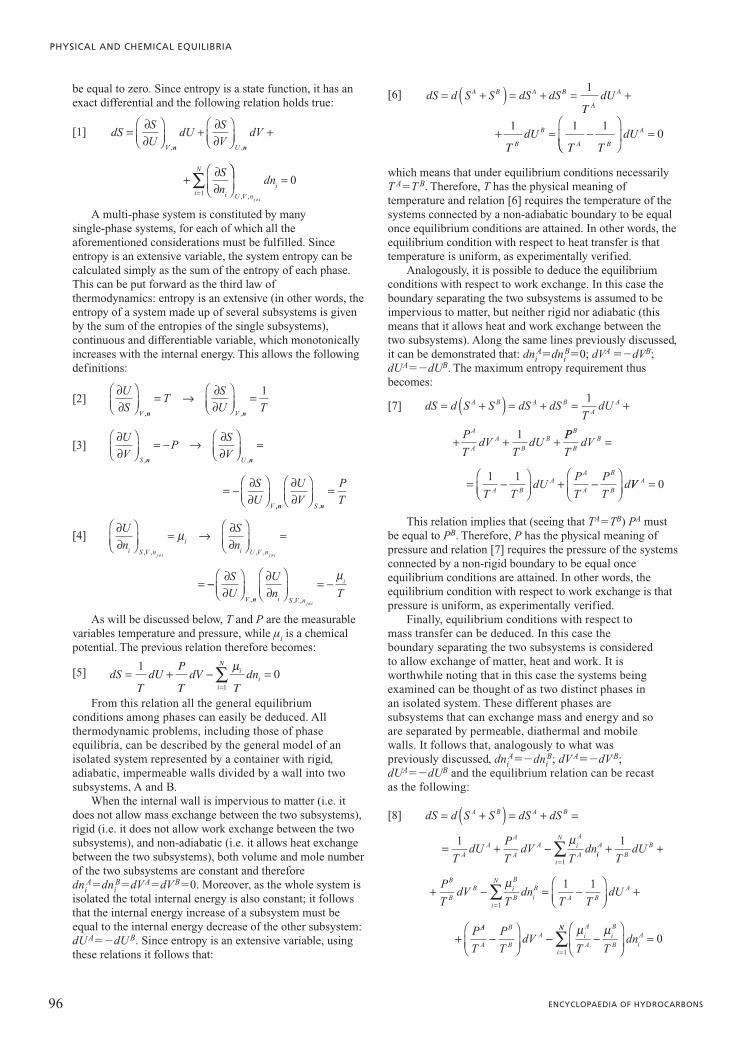
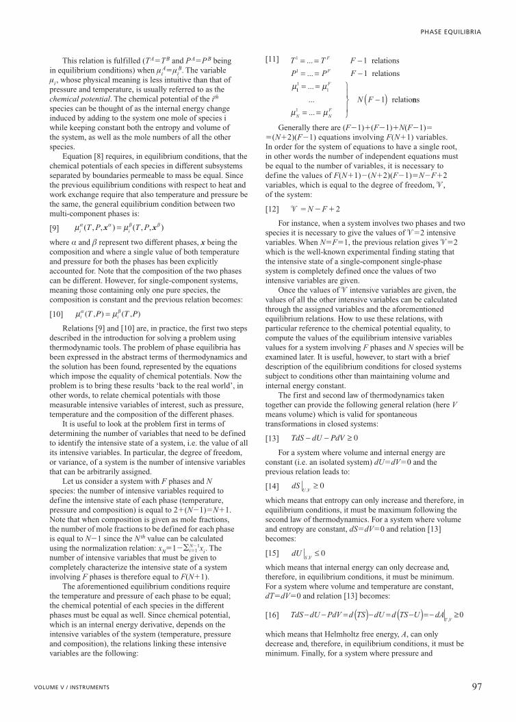

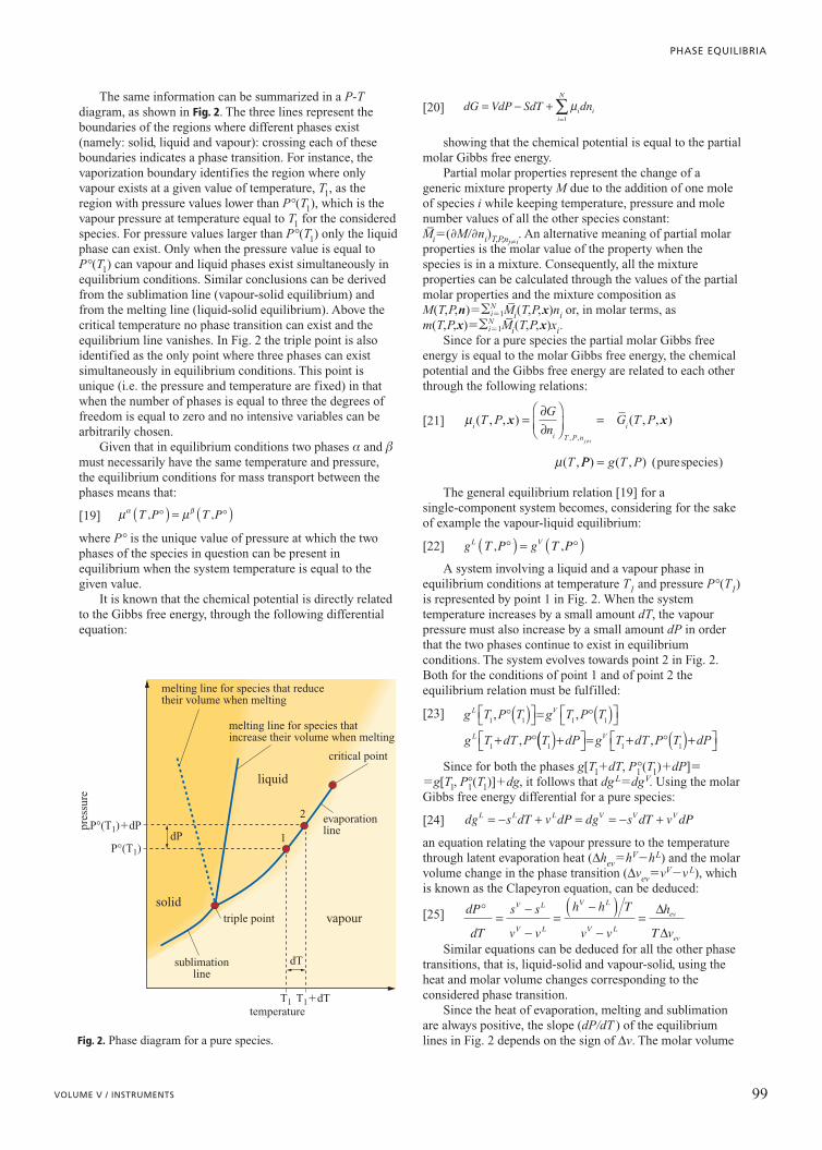
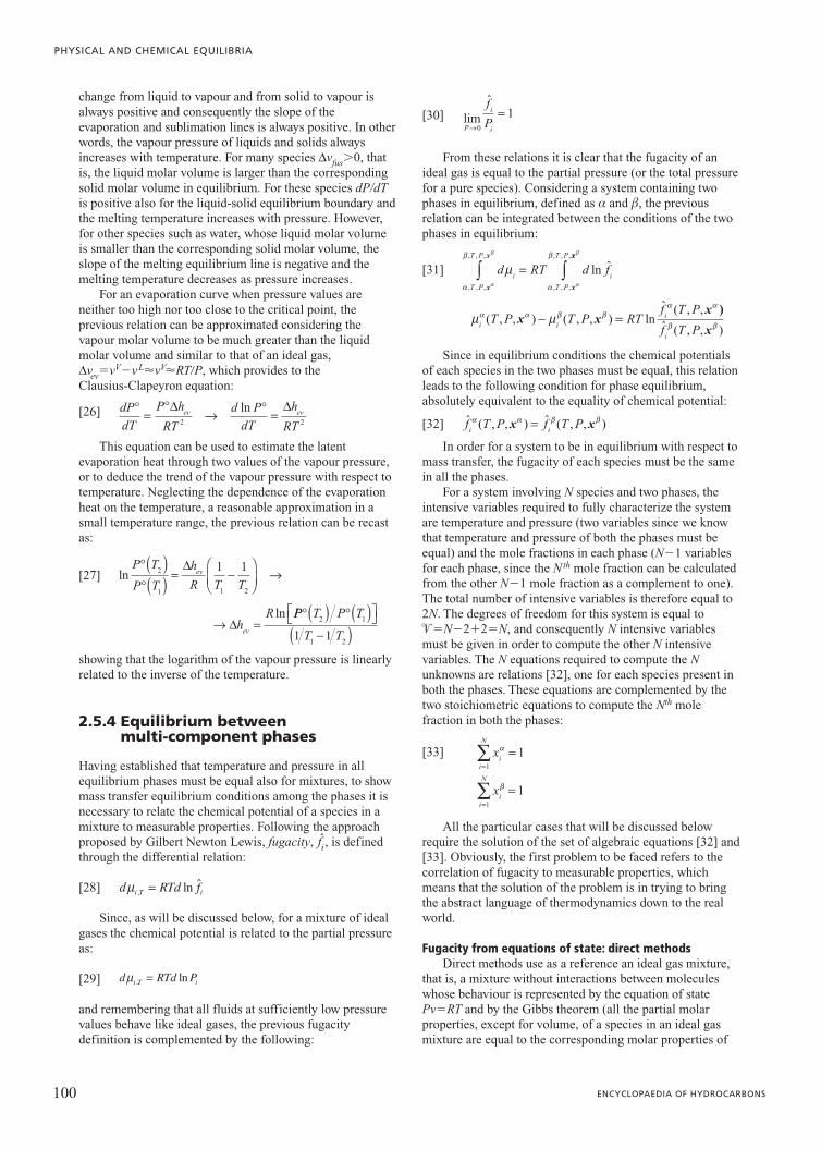

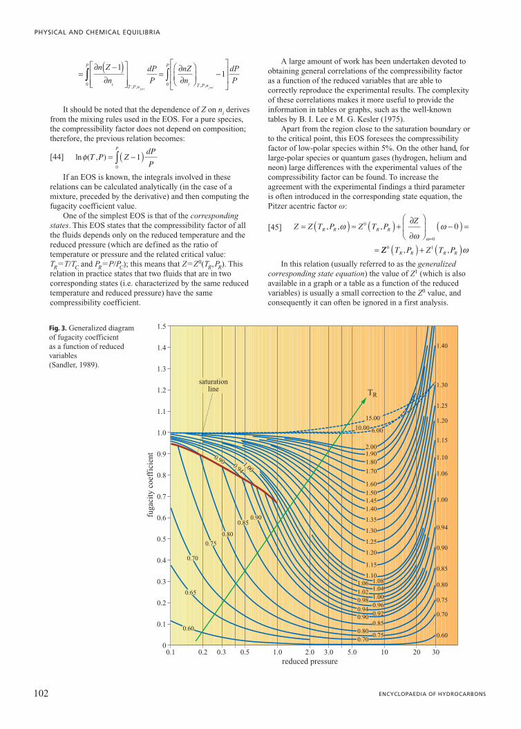
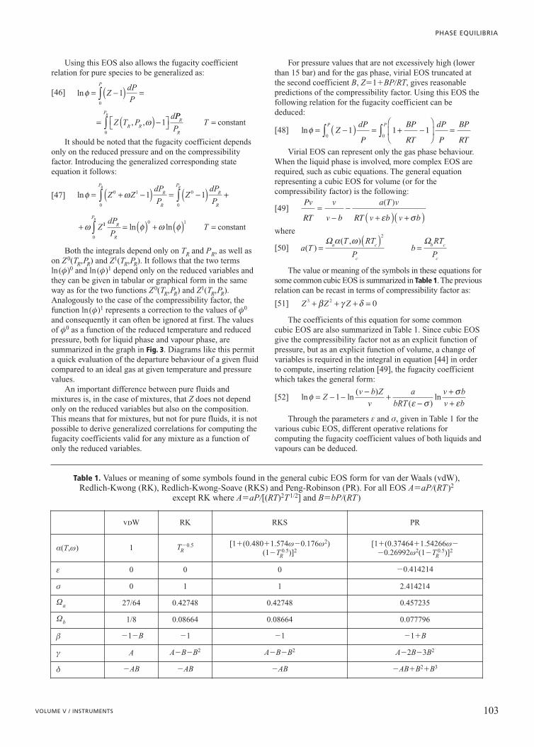


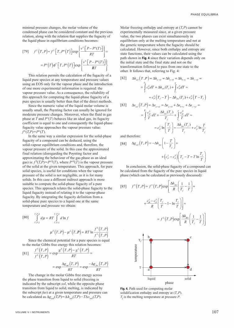


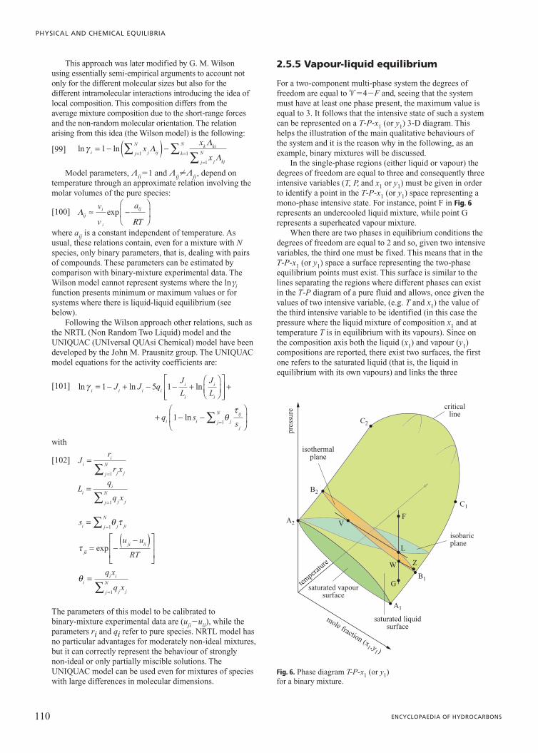

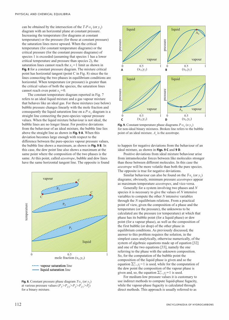


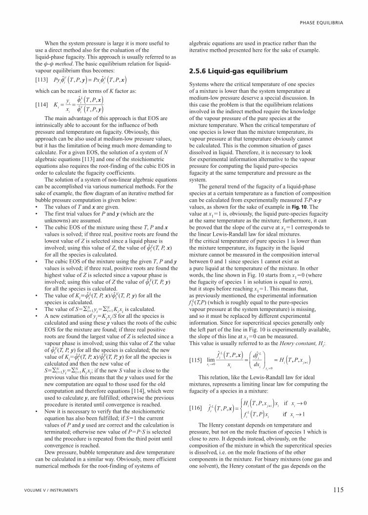
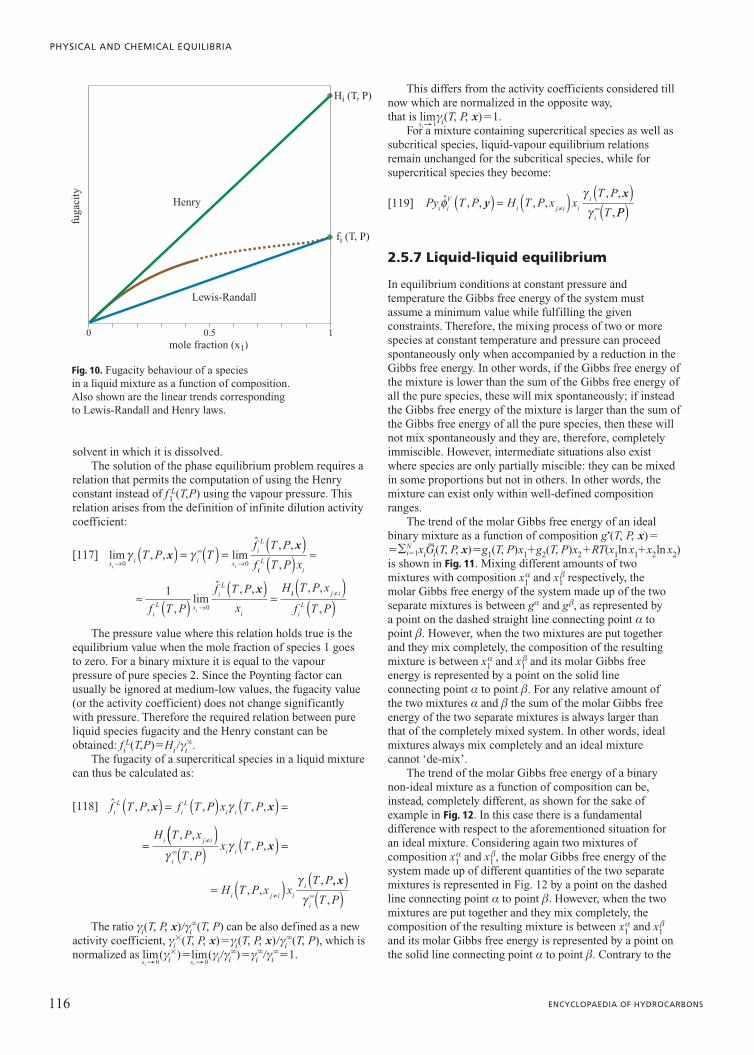


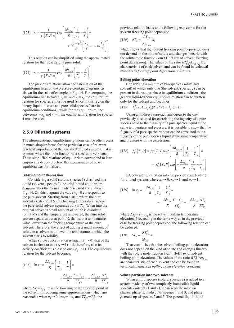


![[Mats Hillert] Phase Equilibria, Phase Diagrams an(BookZZ.org)](https://static.documents.pub/doc/80x56/577c808b1a28abe054a92807/mats-hillert-phase-equilibria-phase-diagrams-anbookzzorg.jpg)


