- 1 - 3. Continuous Random Variables 1) Continuous Distribution If, conceptually, the measurements could come from an interval of possible outcomes, we call them data from a continuous-type population, or more simply, continuous-type data. ‣ Histogram A histogram is a graphical display of tabular frequencies, shown as adjacent rectangles. We assume that a sample of n observations, x 1 , ... , x n , from a distribution are observed. If we have cutpoints for class intervals: , then each rectangle has an area equal to the relative frequency f i /n of the observations for the class. That is, the function is defined by for . ※ With a sample size of ≥ , the histogram is an adequate estimate of the distribution that produced your data. Larger provides better accuracy.
Transcript
- 1 -
3. Continuous Random Variables
1) Continuous DistributionIf, conceptually, the measurements could come from an interval of possible outcomes, we call them data from a continuous-type population, or more simply, continuous-type data.
‣ HistogramA histogram is a graphical display of tabular frequencies, shown as adjacent rectangles. We assume that a sample of n observations, x1, ... , xn, from a distribution are observed. If we have cutpoints for class intervals:
,
then each rectangle has an area equal to the relative frequency fi/n of the observations for the class. That is, the function is defined by
for .
※ With a sample size of ≥ , the histogram is an adequate estimate of the distribution that produced your data. Larger provides better accuracy.
- 2 -
Histogram with 5 bins
x
Den
sity
-4 -2 0 2 4 6
0.0
0.1
0.2
0.3
0.4
0.5
Histogram with 10 bins
x
Den
sity
-4 -2 0 2 4
0.0
0.1
0.2
0.3
0.4
0.5
Histogram with 25 bins
x
Den
sity
-4 -2 0 2 4
0.0
0.1
0.2
0.3
0.4
0.5
Histogram with 50 bins
x
Den
sity
-2 0 2 4
0.0
0.1
0.2
0.3
0.4
0.5
- 3 -
93 77 67 72 52 83 66 84 59 63
75 97 84 73 81 42 61 51 91 87
34 54 71 47 79 70 65 57 90 83
58 69 82 76 71 60 38 81 74 69
68 76 85 58 45 73 75 42 93 65
Stems Leaves Frequency Depths
3 4 8 2 2
4 2 7 5 2 4 6
5 2 9 1 4 7 8 8 7 13
6 7 6 3 1 5 9 0 9 8 5 10 23
7 7 2 5 3 1 9 0 6 1 4 6 3 5 13 (13)
8 3 4 4 1 7 3 2 1 5 9 14
9 3 7 1 0 3 5 5
We assume that a sample of n observations, x1, ... , xn, from a distribution are observed.
‣ Empirical rule: If we let and s be a sample mean and a sample standard deviation respectively, and the histogram of these data is bell shaped, then
a) Approximately 68% of the data are in the interval ( ― s, + s).
b) Approximately 95% of the data are in the interval ( ― 2s, + 2s).
c) Approximately 99.7% of the data are in the interval ( ― 3s, + 3s).
‣ Stem-and-leaf displaySay we have the following 50 test scores on a mid term of Math Stat I:
If the leaves are carefully aligned vertically, the table has the same effect as a histogram, but the original numbers are not lost.
- 4 -
** In the depths column, the frequencies are added together from the low end and the high end until the row is reached that contains the median in the ordered display.
‣ Order statisticsFor a sample of n observations (x1, ... , xn), when the observations are ordered from small to large, the resulting ordered data are called the order statistics. The smallest observation is called the first order statistics and the ith smallest observation is called the ith order statistics.
‣ (100p)th sample percentiles (= sample quantile of order p)If (n+1)p is not an integer but is equal to r plus some proper fraction - say, a/b, the (100p)th sample percentile is yr + (a/b) (yr+1 ― yr) = (1 ― a/b)yr + (a/b)yr+1 where n is the number of sample and yr is the rth order statistics.
※ With a sample size of ≥ , the quantiles are adequate estimates, making the qq plot reasonably trustworthy. Larger provides better accuracy.
Example: When there are 50 samples,50th percentile: 51×0.5 = 25.5 and the median is (1 ― 0.5)y25 + 0.5y26.25th percentile: 51×0.25 = 12.75 and the first quartile is (1 ― 0.75)y12 + 0.75y13.
- 5 -
‣ If there are n observations and yr indicates the rth order statistics,midrange : 0.5 (y1 + yn)Trimean : 0.25 (1st quartile) + 0.5 (2nd quartile) + 0.25 (3rd quartile)Range : yn ― y1
Interquartile range (IQR) : (3rd quartile) ― (1st quartile)
‣ (100p)th percentiles of a population (= a population quantile of order p)(100p)th percentile of a population (or quantile of a population) is a number πp such that the area under f(x) to the left of πp is p. The rth order statistic, yr, from n measurements is the 100r/(n+1)th percentile.
p
- 6 -
Example The time X in months until failure of a certain product has the pdf (of the Weibull type):
exp
∞.
Its distribution function is
exp
∞.
Then, the 30th percentile, π0.3, is given by F(π0.3)=0.3 and
exp
⇒
ln
Example The following data were obtained from the Internet data and story library, or DASL, with URL http://lib.stat.cmu.edu/DASL/ at the time of writing this book. The data are scores given by taste testers on cheese, as follows: 12.3,20.9,39,47.9,5.6,25.9,37.3,21.9,18.1,21,34.9,57.2,0.7,25.9,54.9,40.9,15.9,6.4,18,38.9,14,15.2,32,56.7,16.8,11.6,26.5,0.7,13.4, and 5.5.Find a sample quantile of 0.5 order (, 50th percentile or median), and a population quantile of 0.5 order for the corresponding normal distribution.(sol) (i) 50th sample percentile: 20.95 (15th ordered: 20.9 & 16th ordered: 21 & )
- 7 -
(ii) , ⇒ a population quantile of 0.5 : 24.5
‣ quantile-quantile plot (q-q plot).We assume that there are n measurements from some distribution. If we let the rth order statistics be yr and p = r/(n+1), the plot of (πp, yr)for several values of r is called the q-q plot.
※ Remark (Interpreting quantile-quantile plot). a) Compare the data to the straight line. The closer they are to the line, the more they appear as
if produced by the assumed model. b) Data points higher than the line in the upper right suggest that the pdf that produced the data
tends to give more extreme values in the upper tail than does the assumed distribution. c) Data points lower than the line in the upper right suggest that the pdf that produced the data
tends to give less extreme values in the upper tail than does the assumed distribution. d) Pronounced horizontal lines are evidence of discreteness.
- 8 -
Example (q-q plot): theoretical quantiles are calculated under the normality.
-3 -2 -1 0 1 2 3
-3-2
-10
12
Measurements from Normal dist
Theoretical Quantiles
Sam
ple
Qua
ntile
s
-3 -2 -1 0 1 2 3
0.0
0.2
0.4
0.6
0.8
1.0
Measurements from unif dist
Theoretical Quantiles
Sam
ple
Qua
ntile
s*** q-q plot can be used to confirm the assumed distribution.
- 9 -
2) Properties of pdfs
a) ≤ ∞ ∞ ; b) ∞
∞
c) ≤
;
d) ≤ ≤ ≤ ≤
Example Suppose has the following pdf, find the value of ,
ow .
(sol)
. Thus c = 1/4.
Example Suppose that a pdf for is given by
∞
ow.
Confirm the properties of pdfs: (a), (b) and .
- 10 -
(sol) (a)
∞ ≥
(b) ∞
∞
∞
lim→∞
exp
(c)
∞
∞
lim→∞
exp
** We can change the definition of a pdf of a random variable of the continuous type at a finite (actually countable) number of points without altering the distribution of probability.
3) Transformations ‣ support : support of ⇔ , : pdf of
: support of ⇔ , : pdf of
‣ transformation: method 1
- 11 -
Method I to obtain pdf of : cdf technique
, ≤ ≤
Example
: the distance of the selected point from the origin of a circle of radius 1. Let . Find the support of and the cdf of .
(sol) ≤ ≤ ≤ ≤ ≤
SX = { 1 > y > 0 }
Example Let X have the distribution function F(x) of the continuous type that is strictly increasing on
the support a < x < b. Then if Y = F(X), Find a distribution function of Y. (sol) Since F(a) = 0 and F(b) = 1,
‣ transformation: method 2 Method II to obtain pdf of : transformation Suppose that : pdf of and : differentiable function
a) when is a one-to-one differentiable function on
⋅
for ∈ ow
and ∈ (Proof) If it is strictly increasing,
≤ ≤
because g is increasing and
is positive.If it is strictly decreasing,
- 13 -
≤ ≤ ≥
Thus,
because g is decreasing and
is negative.
Example
ow If we define log , find the support of , the Jacobian, pdf of .
(sol) ⋅
Thus, and SY = { y > 0 }
b) Transformation in general cases
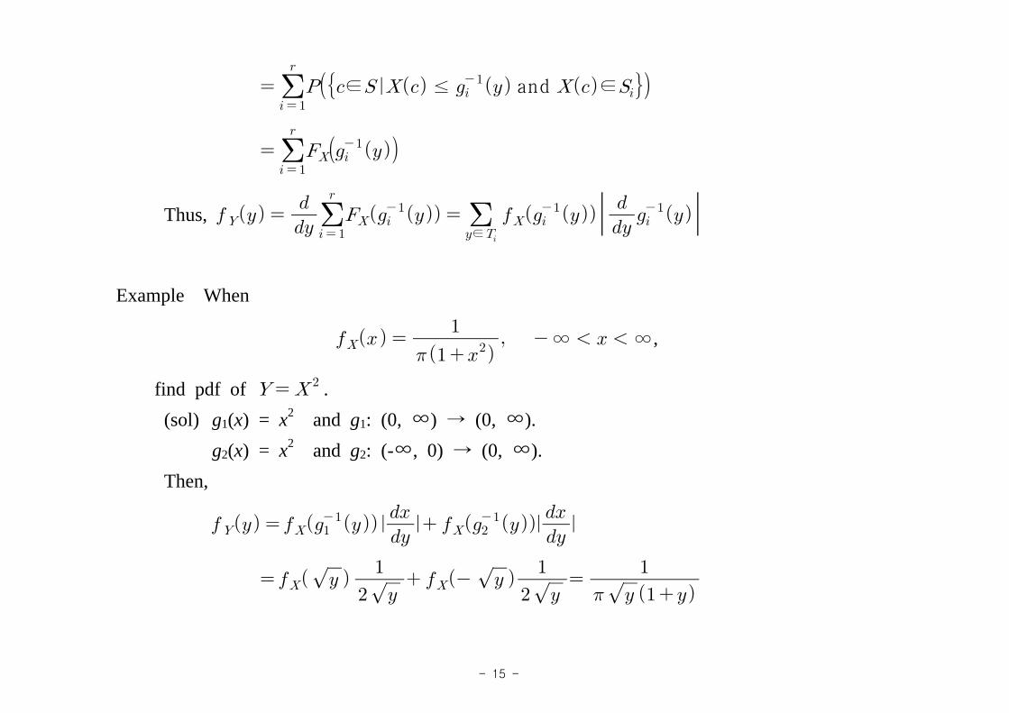
- 14 -
: that is, may be a -to- .
Suppose:
(i) : partition of , ∪
where ∈ and ∈(ii) is a one-to-one function from to (iii) For ∈ , and : differentiable on ,
then,
∈
for ∈
ow.
(Proof) ≤
≤ ∩
∈ ≤ and ∈
∈ ≤ and ∈
- 15 -
∈ ≤ and ∈
Thus,
∈
Example When
∞ ∞,
find pdf of .(sol) g1(x) = x2 and g1: (0, ∞) → (0, ∞).
g2(x) = x2 and g2: (-∞, 0) → (0, ∞).Then,
- 16 -
4) Expectation of a Random Variable
‣ Definition of Expectation : continuous
If has a pdf and ∞
∞
∞ ,
∞
∞
Example Let have the pdf
ow
Find .
(sol)
‣ Expectation of
a) : continuous with pdf
- 17 -
If ∞
∞
∞,
∞
∞
‣ Properties of Expectation a) b)
c) ≥ ⇒ ≥
Example: Let have the pdf
ow Calculate .
(sol)
- 18 -
Example: Divide, at random, a horizontal line segment of length 5 into two parts. If and are the length of the left-hand and right-hand parts respectively, calculate as well as reasonable pdfs of and .
(sol) ≤
,
‣ Mean, Variance, Standard deviation a) Definition
- 19 -
mean :
variance :
standard deviation :
skewness :
kurtosis :
b) Properties (1) ≥
(2)
∵
(3)
Example When have the following pdf, find the mean and the variance,
⋅.
(sol)
- 20 -
- 21 -
Example (example where the mean of does not exist)
⋅∞.
∞
∞
lim
→∞
∞
‣ moment generating function (mgf)
• th moment : • Definition of mgf of :
Let be a continous r.v. such that ∞ for some and . Then,
mgf of :
∞
∞
‣ Relationship between mgf and moment ( )
,
∞
, for some
where exists.
- 22 -
‣ Uniqueness of mgf for some and
⇔ ∀∈
Example Let have the mgf , ∞ ∞. Find the moments of .
(sol)
,
×
Because ′
′′ ,
we can have that
and .
Example Let have the pdf ∞. Then find the mgf of .
(sol)
∞
∞
lim→∞
i f
- 23 -
‣ Remarks: For both the discrete and continuous cases, note that if the rth moment E(Xr) exists and is finite, then the same is true of all lower order moments, E(Xk), k = 1, 2, ..., r ― 1. However, the converse is not true. Moreover, if E(etX) exists and is finite for ―h < t < h, then all moments exist and are finite, but the converse is not necessarily true.
(sol) (i) Let us assume that E(Xk+1) exists, which indicates E|Xk+1| < ∞.
If ≤ , ≤ . If , ≤ .
Thus, ≤ ⇒ ≤ ≤ ∞.
Therefore, if E|Xk+1| < ∞, E|Xk| < ∞ because ≤ ≤ ∞.
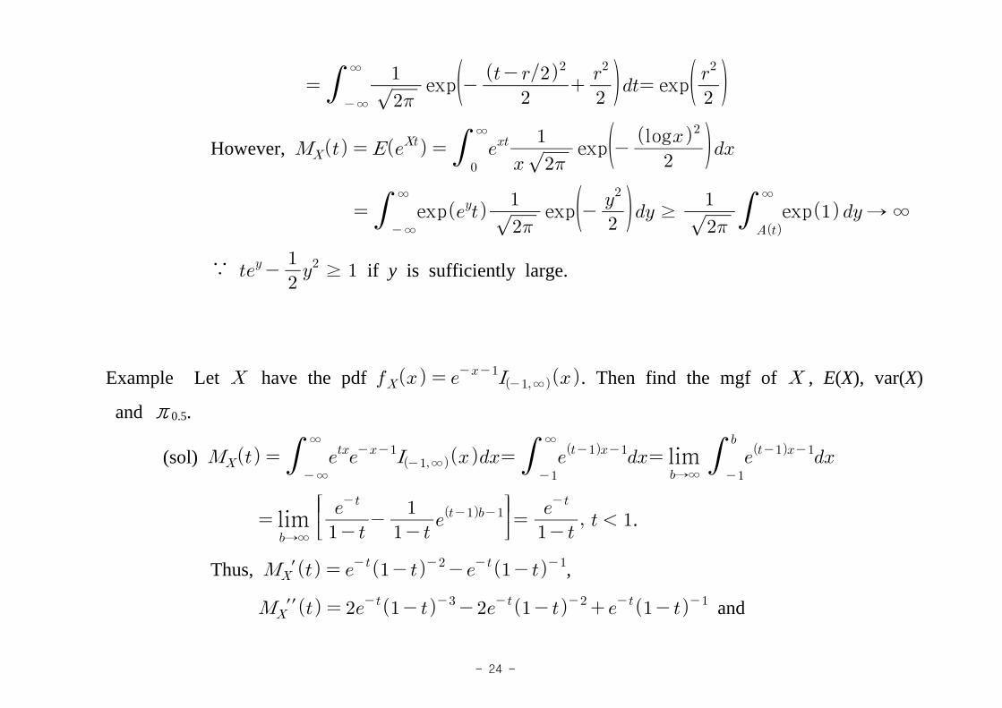
In addition, ≤ ≤ and if ∞ ∞.(ii) If E(etX) exists, we can calculate the rth moment for any r because
.
If follows a log-normal distribution with 0 mean and 1 variance,
explog ∞ .
Then,
∞
explog
∞
∞ exp exp
- 24 -
∞
∞
exp
exp
However,
∞
explog
∞
∞ exp exp
≥
∞ exp → ∞
∵ ≥ if y is sufficiently large.
Example Let have the pdf ∞. Then find the mgf of , E(X), var(X)
and π0.5.
(sol) ∞
∞
∞
∞
lim
→∞
lim→∞
.
Thus, ′ ,′′ and
- 25 -
E(X) = 0 and var(X) = E(X2) - (EX)2 =1.
∞
Thus, and ln .
- 26 -
5) Several distributiona) Uniform distribution ‣ Let the random variable X denote the outcome when a point is selected at random from
∞ ∞. The probability that the point is selected from the interval is
≤
≤
and its pdf is . The random variable X has a uniform distribution and
denoted as U(a, b).
‣ Let X follow U(a, b). Then
and
≠
.
- 27 -
Exponential dist Exp
b) Exponential distribution ‣ We are interested in the waiting times between successive changes. We assume that the number
of changes follows the Possion (λ). If we let W be the waiting time until the first change, the
pdf of W is . If we let
, ∞ and it is called
exponential distribution, ∼Exp .
(sol) ≤ P(a single or more than a change occur in [0, x])
1 ― P(No of changes occuring in [0, x])
and
.
※ Please make sure that the number of changes in [0, x] follows Poisson with xλ.
- 28 -
‣ Let ∼Exp . Then, and
.
(sol)
∞
∞
lim→∞
lim
→∞
′
and′′
. Thus, .
Example Customers arrive in a certain shop according to an approximate Possion process at a mean rate of 20 per hour. What is the probability that the shopkeeper will have to wait more than 5 minutes for the arrival of the first customer?(sol) X ~ P(20) per hour and X ~ P(20/60) per a min. W ~ Exp(3) and
∞
.
Example (no memory property) Suppose that a certain type of electronic component has an
- 29 -
exponential distribution with a mean life of 500 hours. If X denotes the life of this comonent (or the time to failure of this component), then calculate P(X > 900 | X > 300).(sol) X ~ Exp(500).
∞
∞
** The exponential and geometric distribution are the distributions with this forgetfulness property because P(X > b | X > a) = P(X > b - a)
c) Gamma distribution ‣ We are interested in the waiting times until the α changes occurs. We assume that the number
of changes follows the Possion (λ). If we let W be the waiting time, the pdf of W is ≤ P(α or more than α changes occur in [0, x])
1 ― P(fewer than α changes occur in [0, x])
- 30 -
※ Please make sure that the number of changes in [0, x] follows Poisson with λx.
If w < 0, then FW(x) = 0 and fW(x) = 0. The random variable W is said to have a gamma distribution with parameters .
‣ gamma function
∞
for
-
- and - for n: positive integer(sol) (i) From the integration by part,
∞
∞
∞
(ii)
- 31 -
∞
let y = x2/2
∞
∞
∞
(iii) From (i) and (ii),
∞
‣ definition (gamma distribution) ∼ for
⇔
, ∞
• mgf : ,
• mean :
• variance :
• Exp
- 32 -
Gamma dist
(sol) (i) ∞
∞
∞
∞
∞
(let )
(ii) ∞
∞
∞
∞
- 33 -
∞
∞
,
Example Suppose the number of customers per hour arriving at a shop follows a Poisson process with mean 30. That is, if a minute is our unit, then λ = 0.5. What is the probability that the shopkeeper will wait more than 5 minutes until the second customer arrives?
(sol)
∞
∞
∞
or
Example Telephone calls arrive at a switchboard at a mean rate of λ = 2 per minute according to a Poisson process. Let X denote the waiting time in minutes until the fifth call arrives. Then what is the mean and the variance of X?
(sol) ∼. Thus
- 34 -
Chi-square dist
d) Chi-square distribution: a special case of the gamma distribution
‣ definition
∼ for : positive integer ⇔ ∼
⇔
exp , ∞
• mgf : , • mean : • variance :
- 35 -
Example Let have the pdf
∞
ow Find the mean, variance, and mgf.
(sol) ∼ ×
e) The Normal Distribution ‣ definition (normal distribution)
∼, ⇔
exp
, ∞ ∞
• mgf : exp
• mean :
• variance :
• skewness : If the absolute of sample skewness is larger than or equal to 2, the distribution is markedly different from a normal distribution in its asymmetry.
- 36 -
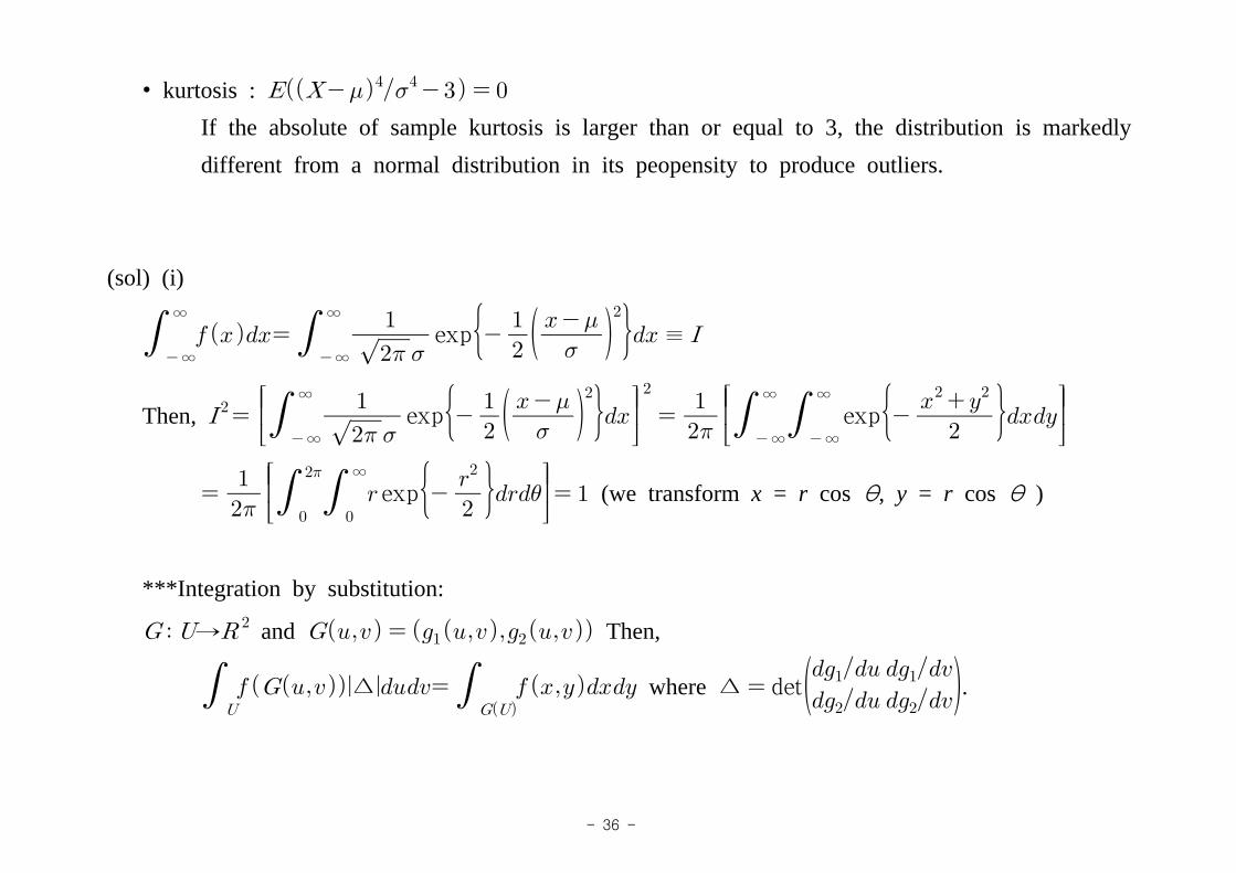
• kurtosis : If the absolute of sample kurtosis is larger than or equal to 3, the distribution is markedly different from a normal distribution in its peopensity to produce outliers.
(sol) (i)
∞
∞
∞
∞
exp
≡
Then,
∞
∞
exp
∞
∞
∞
∞ exp
∞
exp
(we transform x = r cos θ, y = r cos θ )
***Integration by substitution:
→ and Then,
∆
where ∆ det
.
- 37 -
(ii) ∞
∞
exp
∞
∞
exp
∞
∞
exp
exp
∞
∞
exp
exp
∞
∞
exp
‣ standard normal distribution: ∼
,
• cdf : ∞
exp
(sol) exp
- 38 -
⇒
exp
⇒
exp
exp
⇒ exp
exp
⇒ exp
exp
exp
exp
Therefore, ,
Example If X is N(μ, σ2), then find a pdf for Z = (X ― μ)/σ and Z2 = [(X ― μ)/σ]2.
(sol) (i) ≤
≤ ≤
∞
exp
If w = (w ― μ)/σ,
∞
exp
and
exp
(ii)
≤ ≤ ≤
exp
exp
- 39 -
As a result,
exp
exp
exp
Example If X is N(25,36), what is a constant c such that P(|X ― 25| < c) = 0.9544?(sol) P(|X ― 25| < c) = P(―c/6 < (X ― 25)/6 < c/6) = P(―c/6 < Z < c/6)
= FZ(c/6) ― [1 ― FZ(c/6)] = 2FZ(c/6) ― 1 = 0.9544Thus, FZ(c/6) = 0.9772 and c = 12
Example If the cdf of X is
∞
exp ∞ ∞, then what is the mgf of X?
(sol) exp ∵
- 40 -
‣ Mixed type of random variable: the distribution function that is a combination of those for the discrete and continuous types.
‣ Definition of Expectation : continuous on [c1, d1], ... , [cn, dn] and pdf is fj(x) on x ∈ (cj, dj), j = 1, ... , n discrete on {x1, x2, ...} and pmf for each point is p(xi) on xi
Then,
∞
Example Let X have a distribution function defined by
≤ ≤ ≤ ≤
What are the pdf, expectation, and variance of X?
- 41 -
(sol) (i)
≤ As a results, if X = 1 or 2, the X is a discrete type
and the probabilities at X = 1 and 2 are 1/4 and 1/6 respectively. If 0< X < 3 and X is not 1 and 2, the X is a continuous type and its pdf is
≤
.
(ii) ×
×
×
×
Example Consider the following game: An unbiased coin is tossed. If the outcome is a head, the player receives $2. If the outcome is a tail, the player spins a balanced spinner that has a scale from 0 to 1. The player then receives that fraction of a dollar associated with the point selected by the spinner. If X denotes the amount received, what are the cdf, pdf, expectation and variance of X?
- 42 -
(sol) Let Y be the outcome of coin tossing. ≤ ≤ ≤ ≤
≤ ≤ ≤
Thus, ≤
As a results, if X = 2, X is a discrete type and the probability at X = 2 is 1/2. If 0< X < 2, X is a continuous type and its pdf is
≤ ≤ .
×
×
×
×
and
- 43 -
6) Important Inequalities
‣ Let a r.v. and be a positive integer and suppose ∞ .
: integer and ≤ ⇒ ∞ . ‣ Markov's inequality Let ≥ as a function of r.v. ,
≥ ≤ for ∀
(sol) We assume that r.v. is continuous but it can be shown for discrete r.v. by the same way.Let ≥ . Then,
∞
∞
Because ≥
, we can have
≥
≥
- 44 -
‣ Chebyshev's inequality: special case of Makov's inequality
Let , and ∞ ,
≥ ≤
for ∀ .
(sol) In markov inequality, we assume that and . Then
≥ ≥ ≤
Example For any random variable with finite variance, ≤ ≤ . Therefore,
: At most 75% of the data will be within ±2 standard deviations of the mean. : At most 88.9% of the data will be within ±3 standard deviations of the mean. : At most 93.75% of the data will be within ±4 standard deviations of the mean.
‣ Definition (convex function)A function on , ∞≤ ≤∞ is said to be a convex function if
≤ for all ∈ and all .If the above inequality is strict, strictly convex. If is twice differentiable on (a, b), then is convex if and only if ″ ≥ , for all a < x < b.
- 45 -
‣ Jensen's inequality If is convex on an open interval , ≤ . (sol) We assume that has a second derivative. The convexity of means that