Dummy Variables-1 3. DUMMY VARIABLES, NONLINEAR VARIABLES AND SPECIFICATION [1] DUMMY VARIABLES (1) Motivation: • We wish to estimate effects of qualitative regressors on a dependent variable. • Data (GPA1.WF1 or GPA1.TXT from Wooldridge’s Web site): Obs: 141 1. age in years; 2. soph =1 if sophomore 3. junior =1 if junior; 4. senior =1 if senior 5. senior5 =1 if fifth year senior; 6. male =1 if male 7. campus =1 if live on campus; 8. business =1 if business major 9. engineer =1 if engineering major 10. colGPA MSU (Michigan State Univ.) GPA 11. hsGPA high school GPA; 12. ACT 'achievement' score 13. job19 =1 if job <= 19 hours; 14. job20 =1 if job >= 20 hours 15. drive =1 if drive to campus; 16. bike =1 if bicycle to campus 17. walk =1 if walk to campus; 18. voluntr =1 if do volunteer work 19. PC =1 of pers computer at sch 20. greek =1 if fraternity or sorority 21. car =1 if own car 22. siblings =1 if have siblings 23. bgfriend =1 if boy- or girlfriend 24. clubs =1 if belong to MSU club 25. skipped avg lectures missed per week 26. alcohol avg # days per week drink alcohol 27. gradMI =1 if Michigan high school 28. fathcoll =1 if father college grad 29. mothcoll =1 if mother college grad
Transcript
Dummy Variables-1
3. DUMMY VARIABLES, NONLINEAR VARIABLES AND SPECIFICATION
[1] DUMMY VARIABLES
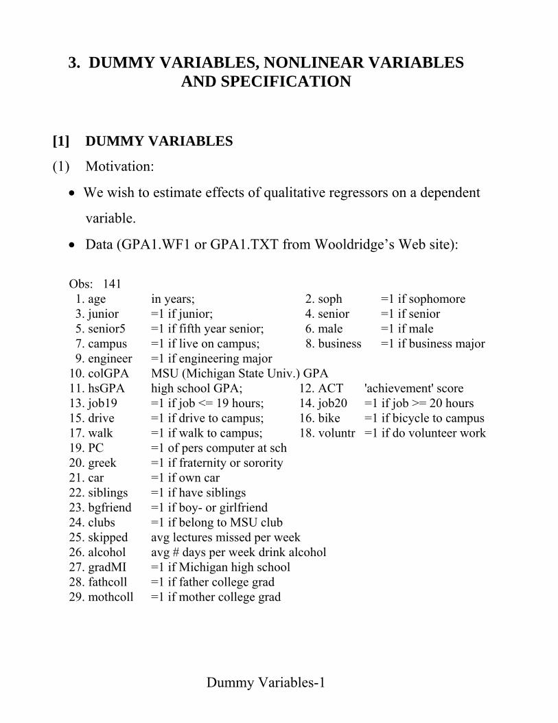
(1) Motivation:
• We wish to estimate effects of qualitative regressors on a dependent
variable.
• Data (GPA1.WF1 or GPA1.TXT from Wooldridge’s Web site):
Obs: 141 1. age in years; 2. soph =1 if sophomore 3. junior =1 if junior; 4. senior =1 if senior 5. senior5 =1 if fifth year senior; 6. male =1 if male 7. campus =1 if live on campus; 8. business =1 if business major 9. engineer =1 if engineering major 10. colGPA MSU (Michigan State Univ.) GPA 11. hsGPA high school GPA; 12. ACT 'achievement' score 13. job19 =1 if job <= 19 hours; 14. job20 =1 if job >= 20 hours 15. drive =1 if drive to campus; 16. bike =1 if bicycle to campus 17. walk =1 if walk to campus; 18. voluntr =1 if do volunteer work 19. PC =1 of pers computer at sch 20. greek =1 if fraternity or sorority 21. car =1 if own car 22. siblings =1 if have siblings 23. bgfriend =1 if boy- or girlfriend 24. clubs =1 if belong to MSU club 25. skipped avg lectures missed per week 26. alcohol avg # days per week drink alcohol 27. gradMI =1 if Michigan high school 28. fathcoll =1 if father college grad 29. mothcoll =1 if mother college grad
Dummy Variables-2
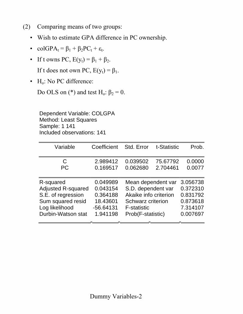
(2) Comparing means of two groups:
• Wish to estimate GPA difference in PC ownership.
• colGPAt = β1 + β2PCt + εt.
• If t owns PC, E(yt) = β1 + β2.
If t does not own PC, E(yt) = β1.
• Ho: No PC difference:
Do OLS on (*) and test Ho: β2 = 0.
Dependent Variable: COLGPA Method: Least Squares Sample: 1 141 Included observations: 141
Variable Coefficient Std. Error t-Statistic Prob.
C 2.989412 0.039502 75.67792 0.0000
PC 0.169517 0.062680 2.704461 0.0077
R-squared 0.049989 Mean dependent var 3.056738Adjusted R-squared 0.043154 S.D. dependent var 0.372310S.E. of regression 0.364188 Akaike info criterion 0.831792Sum squared resid 18.43601 Schwarz criterion 0.873618Log likelihood -56.64131 F-statistic 7.314107Durbin-Watson stat 1.941198 Prob(F-statistic) 0.007697
Dummy Variables-3
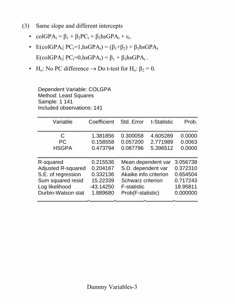
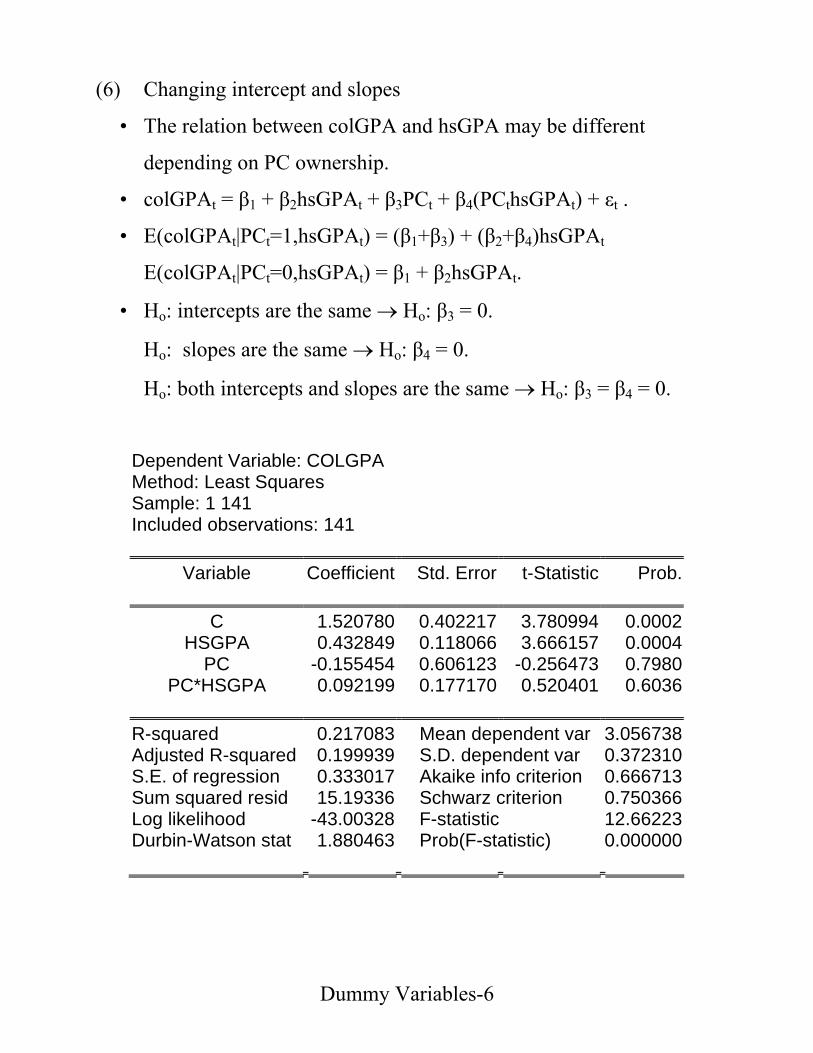
(3) Same slope and different intercepts
• colGPAt = β1 + β2PCt + β3hsGPAt + εt.
• E(colGPAt| PCt=1,hsGPAt) = (β1+β2) + β3hsGPAt
E(colGPAt| PCt=0,hsGPAt) = β1 + β3hsGPAt .
• Ho: No PC difference → Do t-test for Ho: β2 = 0.
Dependent Variable: COLGPA Method: Least Squares Sample: 1 141 Included observations: 141
Variable Coefficient Std. Error t-Statistic Prob.
C 1.381856 0.300058 4.605289 0.0000
PC 0.158558 0.057200 2.771989 0.0063HSGPA 0.473794 0.087796 5.396512 0.0000
R-squared 0.215536 Mean dependent var 3.056738Adjusted R-squared 0.204167 S.D. dependent var 0.372310S.E. of regression 0.332136 Akaike info criterion 0.654504Sum squared resid 15.22339 Schwarz criterion 0.717243Log likelihood -43.14250 F-statistic 18.95811Durbin-Watson stat 1.889680 Prob(F-statistic) 0.000000
Dummy Variables-4
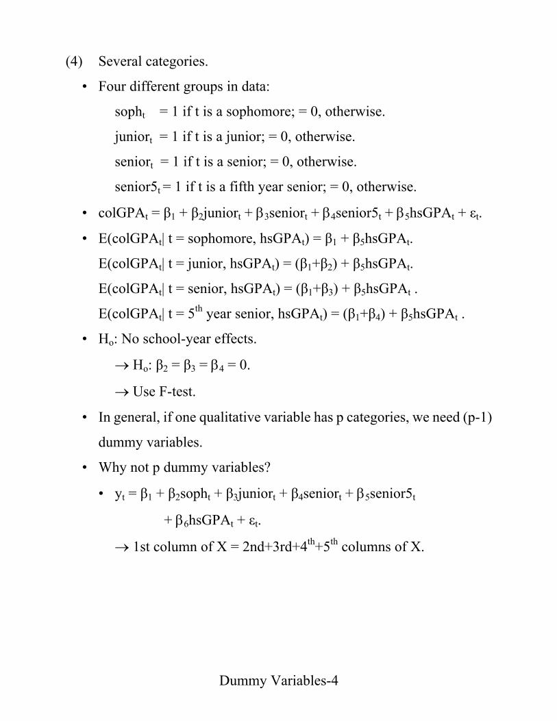
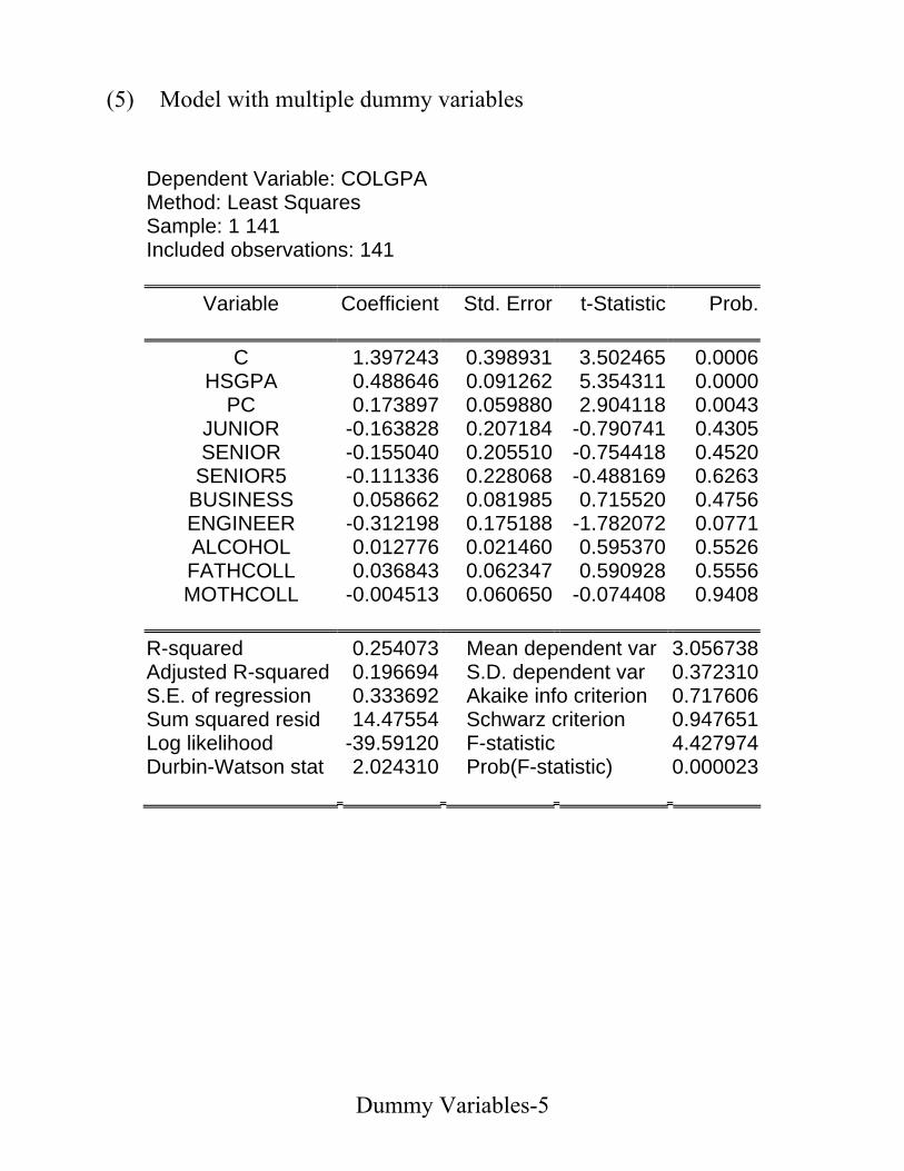
(4) Several categories.
• Four different groups in data:
sopht = 1 if t is a sophomore; = 0, otherwise.
juniort = 1 if t is a junior; = 0, otherwise.
seniort = 1 if t is a senior; = 0, otherwise.
senior5t = 1 if t is a fifth year senior; = 0, otherwise.
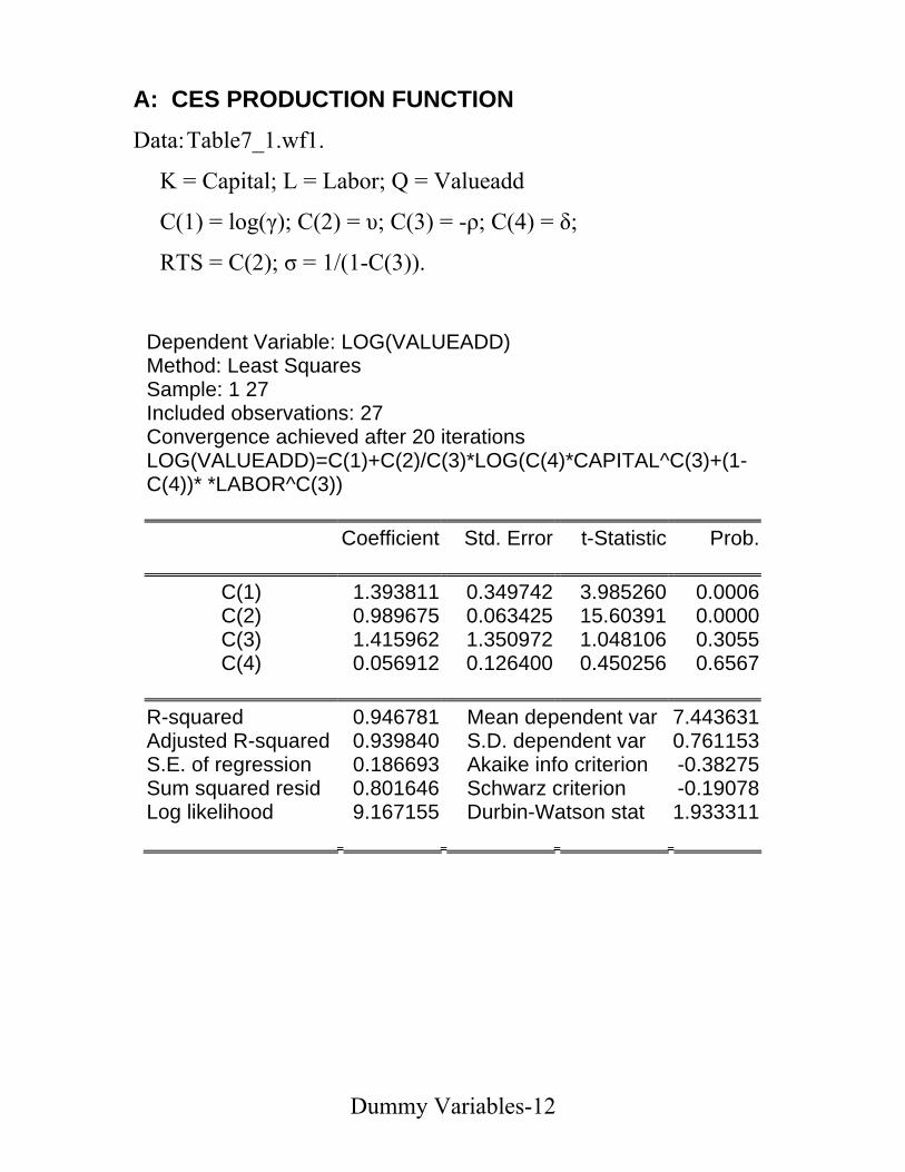
R-squared 0.946781 Mean dependent var 7.443631Adjusted R-squared 0.939840 S.D. dependent var 0.761153S.E. of regression 0.186693 Akaike info criterion -0.38275Sum squared resid 0.801646 Schwarz criterion -0.19078Log likelihood 9.167155 Durbin-Watson stat 1.933311
Dummy Variables-13
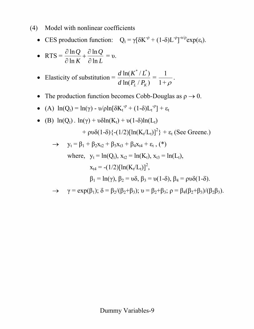
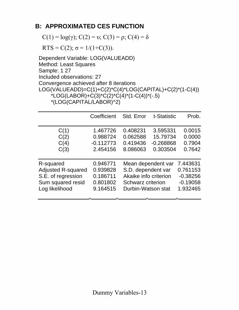
B: APPROXIMATED CES FUNCTION
C(1) = log(γ); C(2) = υ; C(3) = ρ; C(4) = δ
RTS = C(2); σ = 1/(1+C(3)). Dependent Variable: LOG(VALUEADD) Method: Least Squares Sample: 1 27 Included observations: 27 Convergence achieved after 8 iterations LOG(VALUEADD)=C(1)+C(2)*C(4)*LOG(CAPITAL)+C(2)*(1-C(4)) *LOG(LABOR)+C(3)*C(2)*C(4)*(1-C(4))*(-.5) *(LOG(CAPITAL/LABOR)^2)
R-squared 0.946771 Mean dependent var 7.443631Adjusted R-squared 0.939828 S.D. dependent var 0.761153S.E. of regression 0.186711 Akaike info criterion -0.38256Sum squared resid 0.801802 Schwarz criterion -0.19058Log likelihood 9.164515 Durbin-Watson stat 1.932465
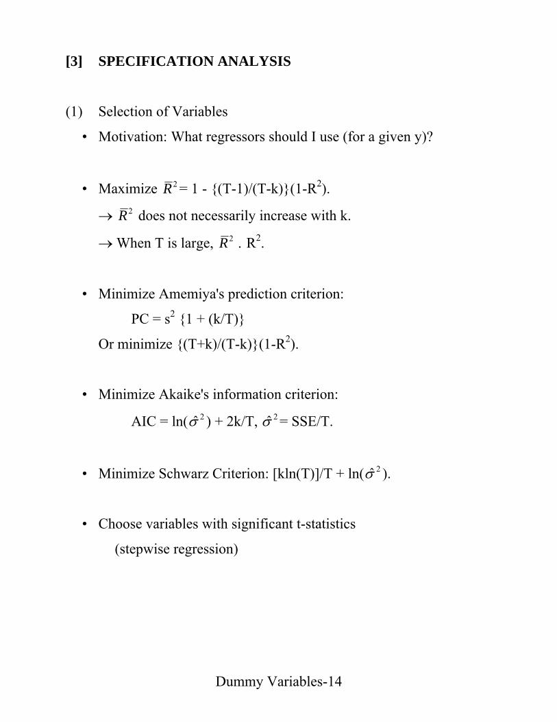
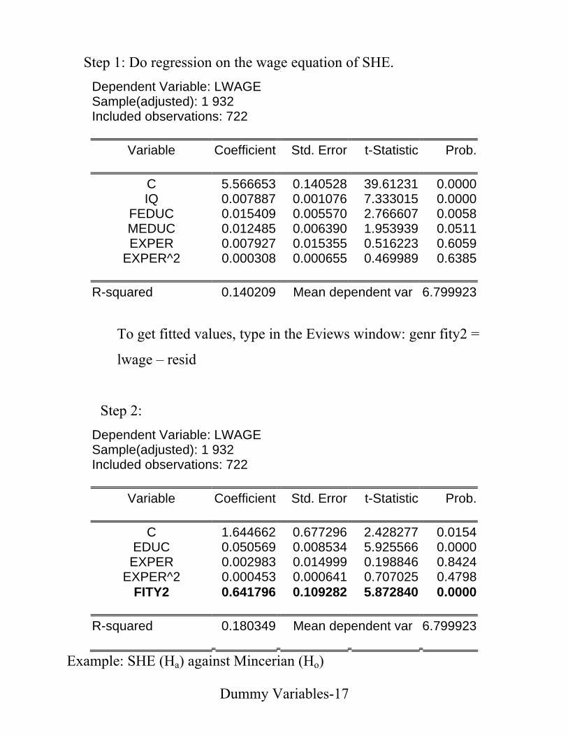
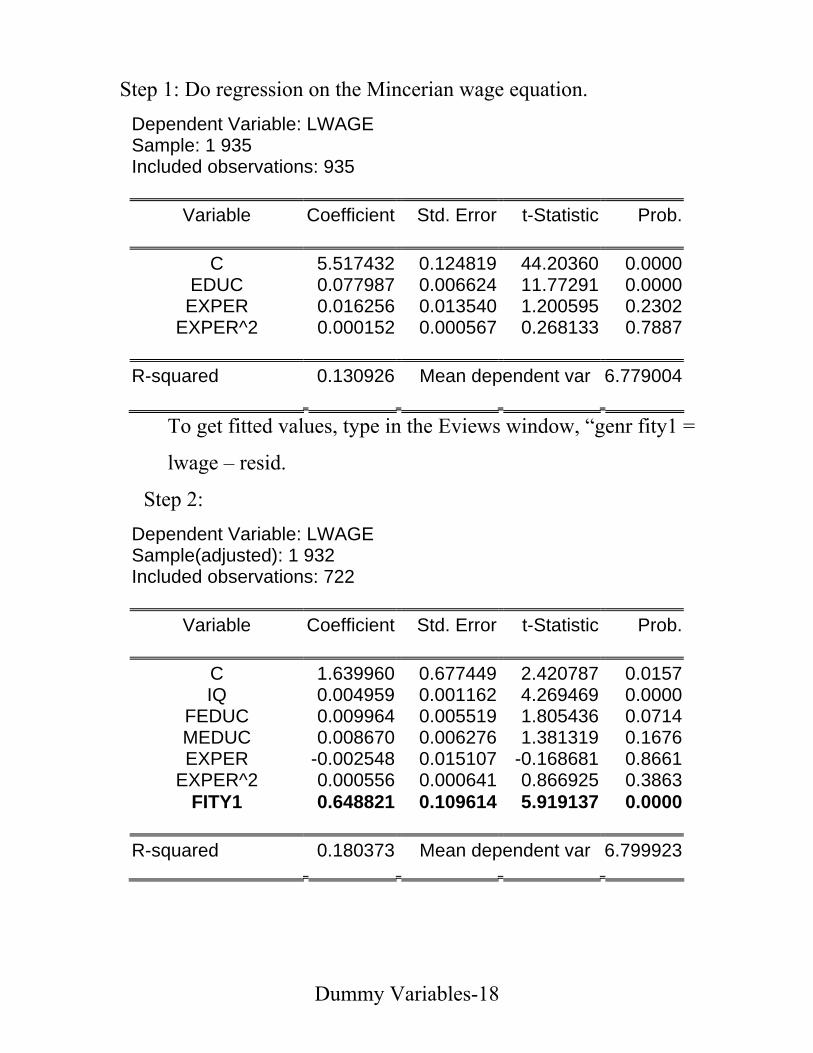
[3] SPECIFICATION ANALYSIS
(1) Selection of Variables
• Motivation: What regressors should I use (for a given y)?
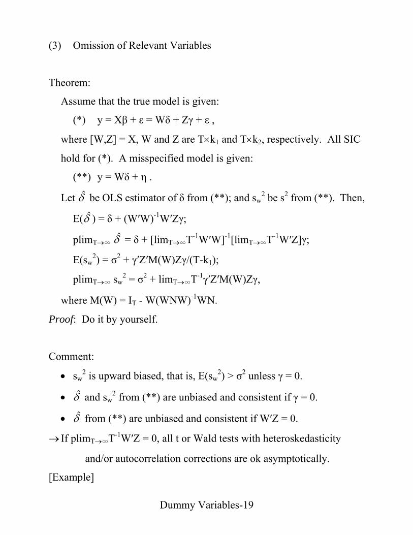
where [W,Z] = X, W and Z are T×k1 and T×k2, respectively. All SIC
hold for (*). A misspecified model is given:
(**) y = Wδ + η .
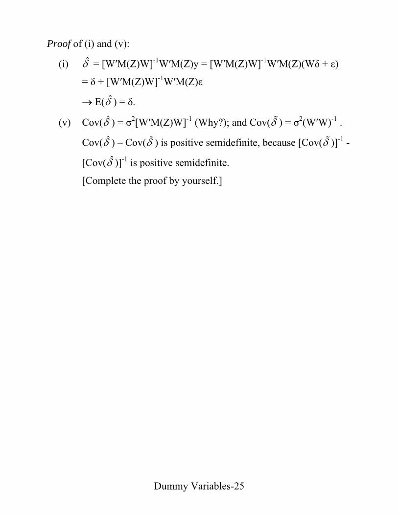
Let δ̂ be OLS estimator of δ from (**); and sw2 be s2 from (**). Then,
E(δ̂ ) = δ + (W′W)-1W′Zγ;
plimT→∞ δ̂ = δ + [limT→∞T-1W′W]-1[limT→∞T-1W′Z]γ;
E(sw2) = σ2 + γ′Z′M(W)Zγ/(T-k1);
plimT→∞ sw2 = σ2 + limT→∞T-1γ′Z′M(W)Zγ,
where M(W) = IT - W(WΝW)-1WΝ.
Proof: Do it by yourself.
Comment:
• sw2 is upward biased, that is, E(sw
2) > σ2 unless γ = 0.
• δ̂ and sw2 from (**) are unbiased and consistent if γ = 0.
• δ̂ from (**) are unbiased and consistent if W′Z = 0.
→ If plimT→∞T-1W′Z = 0, all t or Wald tests with heteroskedasticity
and/or autocorrelation corrections are ok asymptotically.
[Example]
Dummy Variables-19
Dummy Variables-20
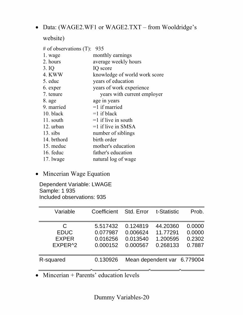
• Data: (WAGE2.WF1 or WAGE2.TXT – from Wooldridge’s
website) # of observations (T): 935 1. wage monthly earnings 2. hours average weekly hours
3. IQ IQ score 4. KWW knowledge of world work score 5. educ years of education
6. exper years of work experience 7. tenure years with current employer 8. age age in years 9. married =1 if married 10. black =1 if black 11. south =1 if live in south 12. urban =1 if live in SMSA 13. sibs number of siblings 14. brthord birth order 15. meduc mother's education 16. feduc father's education 17. lwage natural log of wage
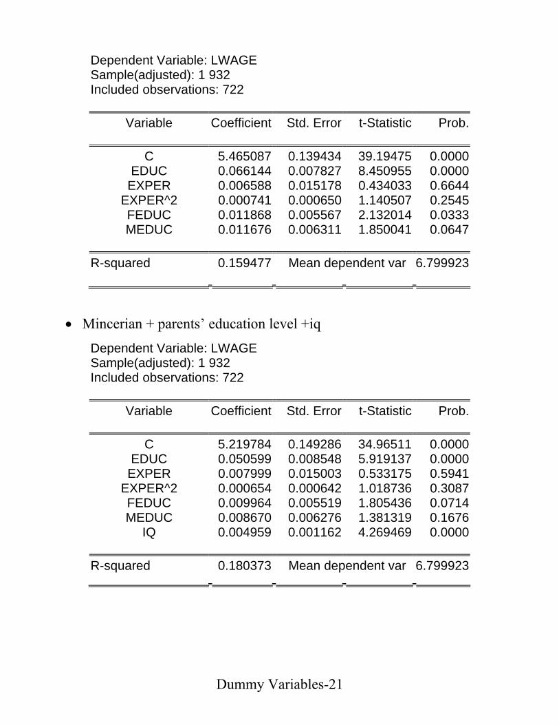
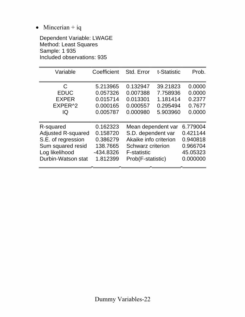
• Mincerian Wage Equation
Dependent Variable: LWAGE Sample: 1 935 Included observations: 935