Class 20: Thurs., Nov. 18

• Specially Constructed Explanatory Variables– Dummy variables for categorical variables– Interactions involving dummy variables

• I will e-mail you HW8 tomorrow. It will be due Tuesday, Nov. 30th.

• Schedule:– Tuesday, Nov. 23rd: One-way ANOVA– Tuesday, Nov. 30th: Review– Thursday, Dec. 2nd: Midterm II– Tuesday, Dec. 7th, Thursday, Dec. 9th: Two-way

ANOVA

Categorical variables

• Categorical (nominal) variables: Variables that define group membership, e.g., sex (male/female), color (blue/green/red), county (Bucks County, Chester County, Delaware County, Philadelphia County).

• How to use categorical variables as explanatory variables in regression analysis:– If the variable has two categories (e.g., sex

(male/female), rain or not rain, snow or not snow), we have defined a variable that equals 1 for one of the categories and 0 for the other category.

Predicting Emergency Calls to the AAA Club

Response Calls Summary of Fit RSquare 0.692384 RSquare Adj 0.584719 Root Mean Square Error 1735.151 Mean of Response 4318.75 Observations (or Sum Wgts)

28

Parameter Estimates Term Estimate Std Error t Ratio Prob>|t| Intercept 3628.7902 2153.788 1.68 0.1076 Average Temperature

-35.63182 51.52383 -0.69 0.4972

Range 133.30434 50.85675 2.62 0.0164 Rain forecast 429.70588 1211.933 0.35 0.7266 Snow forecast 548.80038 1342.27 0.41 0.6870 Weekday -1603.1 876.7378 -1.83 0.0824 Sunday -1847.152 1212.612 -1.52 0.1433 Subzero 3857.6004 1489.803 2.59 0.0175

Rain forecast=1 if rain is in forecast, 0 if notSnow forecast=1 if snow is inforecast, 0 if notWeekday=1 if weekday, 0 ifnot

Comparing Toy Factory Managers

• An analysis has shown that the time required to complete a production run in a toy factory increases with the number of toys produced. Data were collected for the time required to process 20 randomly selected production runs as supervised by three managers (A, B and C). Data in toyfactorymanager.JMP.

• How do the managers compare?

Marginal Comparison

• Marginal comparison could be misleading. We know that large production runs with more toys take longer than small runs with few toys.

Tim

e fo

r R

un

150

200

250

300

a b c

Manager

Oneway Analysis of Time for Run By Manager

• How can we be sure that Manager c’s advantage is not due to simply having supervised smaller production runs?

• Solution: Run a multiple regression in which we include size of the production run as an explanatory variable, along with manager, in order to control for size of the production run.

Run

Siz

e

50

100

150

200

250

300

350

a b c

Manager

Oneway Analysis of Run Size By Manager

Including Categorical Variable in Multiple Regression: Wrong

Approach • We could assign codes to the managers, e.g., Manager

A = 0, Manager B=1, Manager C=2.

• This model says that for the same run size, Manager B is 31 minutes faster than Manager A and Manager C is 31 minutes faster than Manager B.

• This model restricts the difference between Manager A and B to be the same as the difference between Manager B and C – we have no reason to do this.

• If we use a different coding for Manager, we get different results, e.g., Manager B=0, Manager A=1, Manager C=2

Parameter Estimates Term Estimate Std Error t Ratio Prob>|t| Intercept 211.92804 7.212609 29.38 <.0001 Run Size 0.2233844 0.029184 7.65 <.0001 Managernumber -31.03612 3.056054 -10.16 <.0001

Parameter Estimates Term Estimate Std Error t Ratio Prob>|t| Intercept 188.63636 12.73082 14.82 <.0001 Run Size 0.2103122 0.048921 4.30 <.0001 Managernumber2 -5.008207 5.122956 -0.98 0.3324

Manager A 5 min.faster than Manager B

Including Categorical Variable in Multiple Regression: Right

Approach• Create an indicator (dummy) variable for

each category.• Manager[a] = 1 if Manager is A 0 if Manager is not A • Manager[b] = 1 if Manager is B 0 if Manager is not B• Manager[c] = 1 if Manager is C 0 if Manager is not C

• For a run size of length 100, the estimated time for run of Managers A, B and C are

• For the same run size, Manager A is estimated to be on average 38.41-(-14.65)=53.06 minutes slower than Manager B and

38.41-(-23.76)=62.17 minutes slower than Manager C.

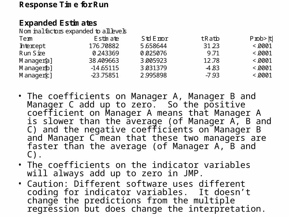
Response Time for Run Expanded Estimates Nominal factors expanded to all levels Term Estimate Std Error t Ratio Prob>|t| Intercept 176.70882 5.658644 31.23 <.0001 Run Size 0.243369 0.025076 9.71 <.0001 Manager[a] 38.409663 3.005923 12.78 <.0001 Manager[b] -14.65115 3.031379 -4.83 <.0001 Manager[c] -23.75851 2.995898 -7.93 <.0001

1*76.230*65.140*41.38100*24.071.176),100|(ˆ

0*76.231*65.140*41.38100*24.071.176),100|(ˆ

0*76.230*65.141*41.38100*24.071.176),100|(ˆ

cManagerRunsizeTimeE

bManagerRunsizeTimeE

aManagerRunsizeTimeE

Categorical Variables in Multiple Regression in JMP

• Make sure that the categorical variable is coded as nominal. To change coding, right clock on column of variable, click Column Info and change Modeling Type to nominal.

• Use Fit Model and include the categorical variable into the multiple regression.

• After Fit Model, click red triangle next to Response and click Estimates, then Expanded Estimates (the initial output in JMP uses a different, more confusing, coding of the dummy variables).

• The coefficients on Manager A, Manager B and Manager C add up to zero. So the positive coefficient on Manager A means that Manager A is slower than the average (of Manager A, B and C) and the negative coefficients on Manager B and Manager C mean that these two managers are faster than the average (of Manager A, B and C).

• The coefficients on the indicator variables will always add up to zero in JMP.

• Caution: Different software uses different coding for indicator variables. It doesn’t change the predictions from the multiple regression but does change the interpretation.

Response Time for Run Expanded Estimates Nominal factors expanded to all levels Term Estimate Std Error t Ratio Prob>|t| Intercept 176.70882 5.658644 31.23 <.0001 Run Size 0.243369 0.025076 9.71 <.0001 Manager[a] 38.409663 3.005923 12.78 <.0001 Manager[b] -14.65115 3.031379 -4.83 <.0001 Manager[c] -23.75851 2.995898 -7.93 <.0001

Equivalence of Using One 0/1 Dummy Variable and Two 0/1 Dummy

Variables when Categorical Variable has two categories

• Parameter Estimates Term Estimate Std Error t Ratio Prob>|t| Intercept 3628.7902 2153.788 1.68 0.1076 Average Temperature

-35.63182 51.52383 -0.69 0.4972

Range 133.30434 50.85675 2.62 0.0164 Rain forecast 429.70588 1211.933 0.35 0.7266 Snow forecast 548.80038 1342.27 0.41 0.6870 Weekday -1603.1 876.7378 -1.83 0.0824 Sunday -1847.152 1212.612 -1.52 0.1433 Subzero 3857.6004 1489.803 2.59 0.0175

Expanded Estimates Nominal factors expanded to all levels Term Estimate Intercept 4321.7173 Average Temperature -35.63182 Range 133.30434 Rain forecast[0] -214.8529 Rain forecast[1] 214.85294 Snow forecast[0] -274.4002 Snow forecast[1] 274.40019 Weekday[0] 801.55002 Weekday[1] -801.55 Sunday[0] 923.57625 Sunday[1] -923.5762 Subzero[0] -1928.8 Subzero[1] 1928.8002

Two models give equivalent predictions. The difference in mean number of Emergency calls between a day with a rain forecast and a day without a rain forecastholding all other variables fixed is 429.71=214.85-(-214.85).

Effect Tests

• Effect test for manager: vs. Haa: not all manager[a],manager[b],manager[c] equal. Null hypothesis is that all : not all manager[a],manager[b],manager[c] equal. Null hypothesis is that all

managers are the same (in terms of mean run time) when run size is held fixed, managers are the same (in terms of mean run time) when run size is held fixed, alternative hypothesis is that not all managers are the same (in terms of mean run alternative hypothesis is that not all managers are the same (in terms of mean run time) when run size is held fixed.time) when run size is held fixed.

• p-value for Effect Test <.0001. Strong evidence that not all managers are the same p-value for Effect Test <.0001. Strong evidence that not all managers are the same when run size is held fixed. when run size is held fixed.

• Note: equivalent to Note: equivalent to because JMP has constraint that manager[a]+manager[b]+manager[c]=0.• Effect test for Run size tests null hypothesis that Run Size coefficient is 0 versus

alternative hypothesis that Run size coefficient isn’t zero. Same p-value as t-test.

Effect Tests Source Nparm DF Sum of Squares F Ratio Prob > F Run Size 1 1 25260.250 94.1906 <.0001 Manager 2 2 44773.996 83.4768 <.0001

Expanded Estimates Nominal factors expanded to all levels Term Estimate Std Error t Ratio Prob>|t| Intercept 176.70882 5.658644 31.23 <.0001 Run Size 0.243369 0.025076 9.71 <.0001 Manager[a] 38.409663 3.005923 12.78 <.0001 Manager[b] -14.65115 3.031379 -4.83 <.0001 Manager[c] -23.75851 2.995898 -7.93 <.0001

][][][:0 cManagerbManageraManagerH

0][][][: cmanagerbmanageramanagerHa

][][][:0 cManagerbManageraManagerH

• Effect tests shows that managers are not equal.• For the same run size, Manager C is best (lowest mean

run time), followed by Manager B and then Manager C.• The above model assumes no interaction between

Manager and run size – the difference between the mean run time of the managers is the same for all run sizes.

Effect Tests Source Nparm DF Sum of Squares F Ratio Prob > F Run Size 1 1 25260.250 94.1906 <.0001 Manager 2 2 44773.996 83.4768 <.0001 Expanded Estimates Nominal factors expanded to all levels Term Estimate Std Error t Ratio Prob>|t| Intercept 176.70882 5.658644 31.23 <.0001 Run Size 0.243369 0.025076 9.71 <.0001 Manager[a] 38.409663 3.005923 12.78 <.0001 Manager[b] -14.65115 3.031379 -4.83 <.0001 Manager[c] -23.75851 2.995898 -7.93 <.0001

Interaction ModelResponse Time for Run Expanded Estimates Nominal factors expanded to all levels Term Estimate Std Error t Ratio Prob>|t| Intercept 179.59191 5.619643 31.96 <.0001 Run Size 0.2344284 0.024708 9.49 <.0001 Manager[a] 38.188168 2.900342 13.17 <.0001 Manager[b] -13.5381 2.936288 -4.61 <.0001 Manager[c] -24.65007 2.887839 -8.54 <.0001 Manager[a]*(Run Size-209.317) 0.0728366 0.035263 2.07 0.0437 Manager[b]*(Run Size-209.317) -0.097651 0.037178 -2.63 0.0112 Manager[c]*(Run Size-209.317) 0.0248147 0.032207 0.77 0.4444

)317.209(*073.0188.38*234.059.179

)317.209(*0*025.0)317.209(*0*098.0)317.209(*1*073.0

0*651.240*538.131*188.38*234.059.179

),|__(ˆ

xx

xxx

x

AManagerxrunsizerunfortimeE

xCManagerxrunsizerunfortimeE

xBManagerxrunsizerunfortimeE

xAManagerxrunsizerunfortimeE

*025.0234.0()317.209*025.0651.2459.179(),|__(ˆ

*)098.0234.0()317.209*098.0538.1359.179(),|__(ˆ

*)073.0234.0()317.209*073.0188.3859.179(),|__(ˆ

Interaction Model in JMP

• To add interactions involving categorical variables in JMP, follow the same procedure as with two continuous variables. Run Fit Model in JMP, add the usual explanatory variables first, then highlight one of the variables in the interaction in the Construct Model Effects box and highlight the other variable in the interaction in the Columns box and then click Cross in the Construct Model Effects box.

Interaction Model• Interaction between run size and Manager: The effect on mean run time

of increasing run size by one is different for different managers.

• Effect Test for Interaction:

• Manager*Run Size Effect test tests null hypothesis that there is no interaction (effect on mean run time of increasing run size is same for all managers) vs. alternative hypothesis that there is an interaction between run size and managers. p-value =0.0333. Evidence that there is an interaction.

259.0025.0234.0),(ˆ),1|__(ˆ

136.0098.0234.0),(ˆ),1|__(ˆ

307.0073.0234.0),(ˆ),1|__(ˆ

CManagerxrunsizeECManagerxrunsizerunfortimeE

BManagerxrunsizeEBManagerxrunsizerunfortimeE

AManagerxrunsizeEAManagerxrunsizerunfortimeE

Effect Tests Source Nparm DF Sum of Squares F Ratio Prob > F Run Size 1 1 22070.614 90.0192 <.0001 Manager 2 2 43981.452 89.6934 <.0001 Manager*Run Size 2 2 1778.661 3.6273 0.0333

• The runs supervised by Manager A appear abnormally time consuming. Manager b has higher initial fixed setup costs than Manager c (186.565>149.706) but has lower per unit production time (0.136<0.259).

xCManagerxrunsizerunfortimeE

xBManagerxrunsizerunfortimeE

xAManagerxrunsizerunfortimeE

*259.0706.149),|__(ˆ

*136.0565.186),|__(ˆ

*307.0498.202),|__(ˆ

Interaction Profile Plot

150

200

250

300

Tim

e

for

Run

150

200

250

300

Tim

e

for

Run

Run Size

a

bc

100 150 200 250 300 350 400

58

345

Manager

a b c

Run S

izeM

anager

Lower left hand plot shows mean time for run vs. run size for the three managersa, b and c.

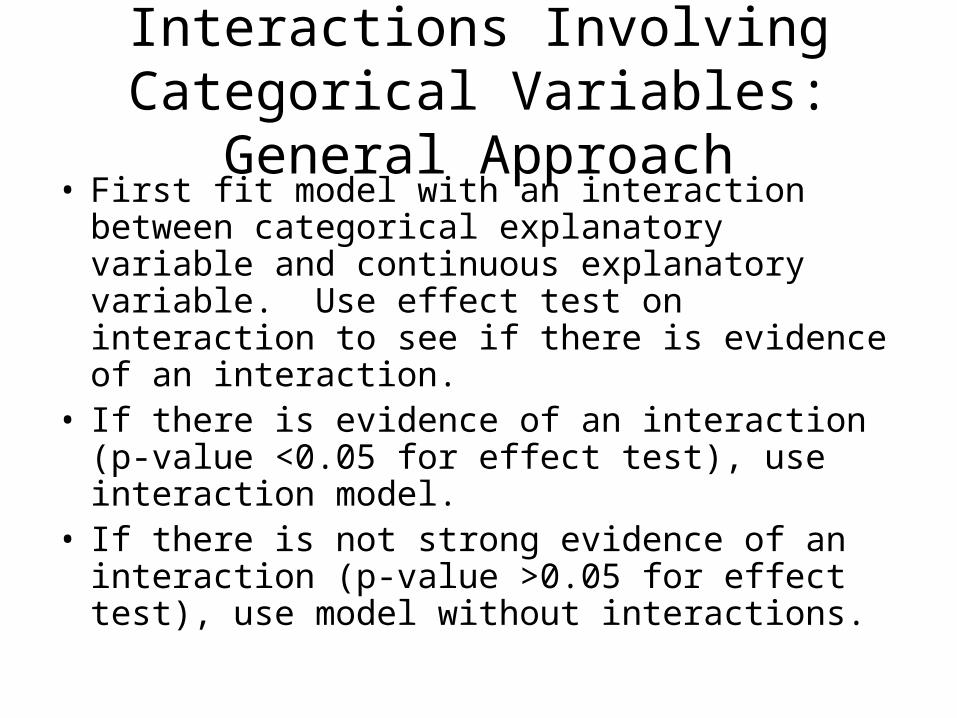
Interactions Involving Categorical Variables: General Approach

• First fit model with an interaction between categorical explanatory variable and continuous explanatory variable. Use effect test on interaction to see if there is evidence of an interaction.

• If there is evidence of an interaction (p-value <0.05 for effect test), use interaction model.

• If there is not strong evidence of an interaction (p-value >0.05 for effect test), use model without interactions.

Example: A Sex Discrimination Lawsuit

• Did a bank discriminatorily pay higher starting salaries to men than to women. Harris Trust and Savings Bank was sued by a group of female employees who accused the bank of paying lower starting salries to women. The data in harrisbank.JMP are the starting salaries for all 32 male and all 61 female skilled, entry-level clerical employees hired by the bank between 1969 and 1977, as well as the education levels and sex of the employees.

• No evidence of an interaction between Sex and Education. Fit model without interactions.

Expanded Estimates Nominal factors expanded to all levels Term Estimate Std Error t Ratio Prob>|t| Intercept 4257.893 422.8744 10.07 <.0001 EDUC 98.923456 31.79614 3.11 0.0025 SEX[FEMALE] -322.6792 68.97647 -4.68 <.0001 SEX[MALE] 322.67916 68.97647 4.68 <.0001 SEX[FEMALE]*(EDUC-12.5054) -36.7929 31.79614 -1.16 0.2503 SEX[MALE]*(EDUC-12.5054) 36.792897 31.79614 1.16 0.2503 Effect Tests Source Nparm DF Sum of Squares F Ratio Prob > F EDUC 1 1 3159890.9 9.6794 0.0025 SEX 1 1 7144342.4 21.8847 <.0001 SEX*EDUC 1 1 437120.8 1.3390 0.2503

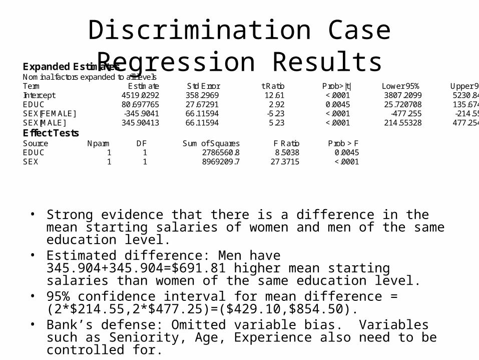
Discrimination Case Regression Results

• Strong evidence that there is a difference in the mean starting salaries of women and men of the same education level.

• Estimated difference: Men have 345.904+345.904=$691.81 higher mean starting salaries than women of the same education level.

• 95% confidence interval for mean difference = (2*$214.55,2*$477.25)=($429.10,$854.50).

• Bank’s defense: Omitted variable bias. Variables such as Seniority, Age, Experience also need to be controlled for.

Expanded Estimates Nominal factors expanded to all levels Term Estimate Std Error t Ratio Prob>|t| Lower 95% Upper 95% Intercept 4519.0292 358.2969 12.61 <.0001 3807.2099 5230.8486 EDUC 80.697765 27.67291 2.92 0.0045 25.720708 135.67482 SEX[FEMALE] -345.9041 66.11594 -5.23 <.0001 -477.255 -214.5533 SEX[MALE] 345.90413 66.11594 5.23 <.0001 214.55328 477.25498 Effect Tests Source Nparm DF Sum of Squares F Ratio Prob > F EDUC 1 1 2786560.8 8.5038 0.0045 SEX 1 1 8969209.7 27.3715 <.0001