3. The Fractional Quantum Hall E↵ect We’ve come to a pretty good understanding of the integer quantum Hall e↵ect and the reasons behind it’s robustness. Indeed, some of the topological arguments in the previous chapter are so compelling that you might think the Hall resistivity of an insulator has to be an integer. But each of these arguments has a subtle loophole and ultimately they hold only for non-interacting electrons. As we will now see, much more interesting things can happen when we include interactions. As with the integer quantum Hall e↵ect, these interesting things were first discovered by experimenters rather than theorists. Indeed, it came as a great surprise to the community when, in 1982, plateaux in the Hall resistivity were seen at non-integer filling fractions. These plateaux were first seen at filling fraction ⌫ = 1 3 and 2 3 , and later at ⌫ = 1 5 , 2 5 , 3 7 , 4 9 , 5 9 , 3 5 ,... in the lowest Landau level and ⌫ = 4 3 , 5 3 , 7 5 , 5 2 , 12 5 , 13 5 ,... in higher Landau levels, as well as many others. There are now around 80 quantum Hall plateaux that have been observed. A number of these are shown below 13 : There’s two things that we can say immediately. First, the interactions between elec- trons must be playing some role. And second, the answer to why these plateaux form is likely to be very hard. Let’s see why. Suppose, for the sake of argument, that we have ⌫ < 1 so that the lowest Landau level is partially filled. Each Landau level can house N = AB/Φ 0 (spin polarised) 13 This data is from R. Willett, J. P. Eisenstein, H. L. Stormer, D. C. Tsui, A. C. Gossard and H. English “Observation of an Even-Denominator Quantum Number in the Fractional Quantum Hall E↵ect”, Phys. Rev. Lett. 59, 15 (1987). – 74 –
Transcript
3. The Fractional Quantum Hall E↵ect
We’ve come to a pretty good understanding of the integer quantum Hall e↵ect and
the reasons behind it’s robustness. Indeed, some of the topological arguments in the
previous chapter are so compelling that you might think the Hall resistivity of an
insulator has to be an integer. But each of these arguments has a subtle loophole and
ultimately they hold only for non-interacting electrons. As we will now see, much more
interesting things can happen when we include interactions.
As with the integer quantum Hall e↵ect, these interesting things were first discovered
by experimenters rather than theorists. Indeed, it came as a great surprise to the
community when, in 1982, plateaux in the Hall resistivity were seen at non-integer
filling fractions. These plateaux were first seen at filling fraction ⌫ = 1
3
and 2
3
, and
later at ⌫ = 1
5
, 25
, 37
, 49
, 59
, 35
, . . . in the lowest Landau level and ⌫ = 4
3
, 53
, 75
, 52
, 12
5
, 13
5
, . . .
in higher Landau levels, as well as many others. There are now around 80 quantum
Hall plateaux that have been observed. A number of these are shown below13:
There’s two things that we can say immediately. First, the interactions between elec-
trons must be playing some role. And second, the answer to why these plateaux form
is likely to be very hard. Let’s see why.
Suppose, for the sake of argument, that we have ⌫ < 1 so that the lowest Landau
level is partially filled. Each Landau level can house N = AB/�0
(spin polarised)
13This data is from R. Willett, J. P. Eisenstein, H. L. Stormer, D. C. Tsui, A. C. Gossard andH. English “Observation of an Even-Denominator Quantum Number in the Fractional Quantum HallE↵ect”, Phys. Rev. Lett. 59, 15 (1987).
– 74 –
E E
Figure 25: Density of states in the lowest
Landau level without interactionsFigure 26: ...and with interactions (with
only a single gap at ⌫ = 1/3 shown.
electrons, where B is the magnetic field and A is the area of the sample. This is a
macroscopic number of electrons. The number of ways to fill ⌫N of these states is� N⌫N
�which, using Stirling’s formula, is approximately
�1
⌫
�⌫N �1
1�⌫
�(1�⌫)N
. This is a
ridiculously large number: an exponential of an exponential. The ground state of any
partially filled Landau level is wildly, macroscopically degenerate.
Now consider the e↵ect of the Coulomb interaction between electrons,
VCoulomb
=e2
4⇡✏0
|ri � rj|(3.1)
On general grounds, we would expect that such an interaction would lift the degen-
eracy of ground states. But how to pick the right one? The approach we’re taught
as undergraduates is to use perturbation theory. But, in this case, we’re stuck with
extraordinarily degenerate perturbation theory where we need to diagonalise a macro-
scopically large matrix. That’s very very hard. Even numerically, no one can do this
for more than a dozen or so particles.
We can, however, use the experiments to intuit what must be going on. As we
mentioned above, we expect the the electron interactions to lift the degeneracy of the
Landau level, resulting in a spectrum of states of width ⇠ ECoulomb
. The data would
be nicely explained if this spectrum had gaps at the filling fractions ⌫ where Hall states
are seen. In the picture above, we’ve depicted just a single gap at ⌫ = 1/3. Presumably
though there are many gaps at di↵erent fractions: the more prominent the plateaux,
the larger the gap.
Then we can just re-run the story we saw before: we include some disorder, which
introduces localised states within the gap, which then gives rise both to the plateaux
– 75 –
in ⇢xy and the observed ⇢xx = 0. The bigger the gap, the more prominent the observed
plateaux. This whole story requires the hierarchy of energy scales,
~!B � ECoulomb
� Vdisorder
We will assume in what follows that this is the case. The question that we will focus
on instead is: what is the physics of these fractional quantum Hall states?
In what follows, we will take advantage of the di�culty of a direct theoretical attack
on the problem to give us license to be more creative. As we’ll see, the level of rigour
in the thinking about the fractional quantum Hall e↵ect is somewhat lower than that
of the integer e↵ect. Instead, we will paint a compelling picture, using a number of
di↵erent approaches, to describe what’s going on.
3.1 Laughlin States
The first approach to the fractional quantum Hall e↵ect was due to Laughlin14, who
described the physics at filling fractions
⌫ =1
m
with m an odd integer. As we’ve explained above, it’s too di�cult to diagonalise the
Hamiltonian exactly. Instead Laughlin did something very bold: he simply wrote down
the answer. This was motivated by a combination of physical insight and guesswork.
As we will see, his guess isn’t exactly right but, it’s very close to being right. More
importantly, it captures all the relevant physics.
3.1.1 The Laughlin Wavefunction
Laughlin’s wavefunction didn’t come out of nowhere. To motivate it, let’s start by
considering an illuminating toy model.
Two Particles
Consider two particles interacting in the lowest Landau level. We take an arbitrary
central potential between them,
V = V (|r1
� r2
|)
Recall that in our first courses on classical mechanics we solve problems like this by
using the conservation of angular momentum. In quantum physics, this means that we
14The original paper is “Anomalous quantum Hall e↵ect: An Incompressible quantum fluid withfractionally charged excitations” , Phys. Rev. Lett. 50 (1983) 1395.
– 76 –
work with eigenstates of angular momentum. As we saw in Section 1.4, if we want to
talk about angular momentum in Landau levels, we should work in symmetric gauge.
The single particle wavefunctions in the lowest Landau level take the form (1.30)
m ⇠ zme�|z|2/4l2B
with z = x � iy. These states are localised on a ring of radius r =p2mlB. The
exponent m of these wavefunctions labels the angular momentum. This can be seen by
acting with the angular momentum operator (1.31),
J = i~✓x@
@y� y
@
@x
◆= ~(z@ � z@) ) J m = ~m m
Rather remarkably, this information is enough to solve our two-particle problem for
any potential V ! As long as we neglect mixing between Landau levels (which is valid
if ~!B � V ) then the two-particle eigenstates for any potential must take the form
= (z1
+ z2
)M(z1
� z2
)me�(|z1|2+|z2|2)/4l2B
where M,m are non-negative integers, with M determining the angular momentum of
the centre of mass, and m the relative angular momentum. Note that here, and below,
we’ve made no attempt to normalise the wavefunctions.
It’s surprising that we can just write down eigenfunctions for a complicated potentials
V (r) without having to solve the Schrodinger equation. It’s even more surprising that
all potentials V (r) have the same energy eigenstates. It is our insistence that we lie in
the lowest Landau level that allows us to do this.
Many-Particles
Unfortunately, it’s not possible to generalise arguments similar to those above to
uniquely determine the eigenstates for N > 2 particles. Nonetheless, on general
grounds, any lowest Landau level wavefunction must take the form,
(z1
, . . . , zn) = f(z1
, . . . , zN)e�
PN
i=1 |zi|2/4l2B (3.2)
for some analytic function f(z). Moreover, this function must be anti-symmetric under
exchange of any two particle zi $ zj, reflecting the fact that the underlying electrons
are fermions.
– 77 –
Laughlin’s proposal for the ground state wavefunction at filling fraction ⌫ = 1/m is:
(zi) =Yi<j
(zi � zj)me�
Pn
i=1 |zi|2/4l2B (3.3)
Clearly this is anti-symmetric when m is an odd integer. For m an even integer, it
can be thought of as a quantum Hall state for bosons. The pre-factor vanishes with
a zero of order m whenever two electrons come together. Meanwhile, the exponential
factor decreases quickly whenever the electrons get too far away from the origin. The
wavefunction is peaked on configurations that balance these two e↵ects.
Let’s first show that the wavefunction has the desired filling fraction. To do this,
focus on what the wavefunction is telling us about a single particle, say z1
. The terms
that depend on z1
in the pre-factor of the Laughlin wavefunction are
Yi<j
(zi � zj)m ⇠
NYi=2
(z1
� zi)m
which tells us that there are m(N � 1) powers of z1
. This, in turn, tells us that the
maximum angular momentum of the first particle is m(N � 1) and so its maximum
radius is R ⇡p2mNlB. Correspondingly, the area of the droplet is A ⇡ 2⇡mNl2B
(where we’ve replaced N � 1 with N). Recall that the number of states in the full
Landau level is AB/�0
= A/2⇡l2B ⇡ mN . This argument gives us the filling fraction
⌫ =1
m(3.4)
as promised.
It can be shown numerically that, at least for small numbers of particles, this wave-
function has greater than 99% overlap with the true ground state arising arising from
both the Coulomb repulsion (3.1) as well as a number of other repulsive potentials V .
Heuristically this occurs because the wavefunction has a zero of order m whenever two
electrons coincide. Of course, a single zero is guaranteed by Pauli exclusion, but the
Laughlin wavefunction does more. It’s as if each electron carves out a space around it
which helps it minimise the for repulsive potentials.
The high numerical overlap with the true ground state is often put forward as strong
evidence for the veracity of the Laughlin wavefunction. While it’s certainly impressive,
this isn’t the reason that the Laughlin wavefunction is interesting. Finding the ground
state numerically is di�cult and can only be done for a couple of dozen particles. While
this may provide 99.99% overlap with the Laughlin wavefunction, by the time we get
– 78 –
to 1011 particles or so, the overlap is likely to be essentially zero. Instead, we should
think of the Laughlin wavefunctions as states which lie in the same “universality class”
as the true ground state. As we explain in more detail in Section 3.2, this means that
the states have the same fractional excitations and the same topological order.
The Fully Filled Landau Level
From the arguments above, the Laughlin state (3.3) with m = 1 should describe a
completely filled Landau level. But this is something we can compute in the non-
interacting picture and it provides a simple check on the Laughlin ansatz.
Let us first review how to build the many-particle wavefunction for non-interacting
electrons. Suppose that N electrons sit in states i(x), with 1 = 1, . . . , N . Because
the electrons are fermions, these states must be distinct. To build the many-particle
wavefunction, we need to anti-symmetrise over all particles. This is achieved by the
Slater determinant,
(xi) =
�����������
1
(x1
) 1
(x2
) . . . 1
(xN)
2
(x1
) 2
(x2
) . . . 2
(xN)...
...
N(x1
) N(x2
) . . . N(xN)
�����������(3.5)
We can now apply this to the lowest Landau level, with the single-particle states built
up with successive angular momentum quantum numbers
m(z) ⇠ zm�1e�|z|2/4l2B m = 1, . . . , N
The resulting Slater determinant gives a state of the general form (3.2), with f(zi)
given by a function known as the Vandermonde determinant,
f(zi) =
�����������
z01
z02
. . . z0N
z1
z2
. . . z3
......
zN�1
1
zN�1
2
. . . zN�1
N
�����������=Yi<j
(zi � zj)
To see that the determinant is indeed given by the product factor, note thatQ
i<j(zi�zj)
is the lowest order, fully anti-symmetric polynomial (because any such polynomial must
have a factor (zi�zj) for each pair i 6= j). Meanwhile, the determinant is also completely
anti-symmetric and has the same order as the product factor. This ensures that they
must be equal up to an overall numerical factor which can be checked to be 1. We see
that m = 1 Laughlin state does indeed agree with the wavefunction for a completely
filled lowest Landau level.
– 79 –
The Competing Phase: The Wigner Crystal
The Laughlin state should be thought of as a liquid phase of electrons. In fact, strictly
speaking, it should be thought of as an entirely new phase of matter, distinguished by
a property called topological order which we’ll discuss in Section 3.2.4. But, if you’re
looking for a classical analogy, a liquid is the best.
There is a competing solid phase in which the electrons form a two-dimensional
triangular lattice, known as a Wigner crystal. Indeed, before the discovery of the
quantum Hall e↵ect, it was thought that this would be the preferred phase of electrons
in high magnetic fields. It’s now known that the Wigner crystal has lower energy than
the Laughlin state only when the densities of electrons are low. It is observed for filling
fractions ⌫ . 1
7
3.1.2 Plasma Analogy
The Laughlin wavefunctions (3.3) are very easy to write down. But it’s hard to actually
compute with them. The reason is simple: they are wavefunctions for a macroscopic
number of particles which means that if we want to compute expectation values of
operators, we’re going to have to do a macroscopic number of integralsRd2zi. And
that’s di�cult.
For example, suppose that we want to figure out the average density of the quantum
Hall droplet. We need to compute the expectation value of the density operator
n(z) =NXi=1
�(z � zi)
This is given by
h |n(z)| i =R QN
i=1
d2zi n(z)P [zi]QNi=1
d2zi P [zi](3.6)
where we’ve introduced the un-normalised probability density associated to the Laugh-
lin wavefunction
P [zi] =Yi<j
|zi � zj|2ml2mB
e�P
i
|zi
|2/2l2B (3.7)
The integrals in (3.6) are hard. How to proceed?
– 80 –
The key observation is that the expectation value (3.6) has the same formal structure
as the kind of things we compute in classical statistical mechanics, with the denominator
interpreted as the partition function,
Z =NYi=1
d2zi P [zi]
Indeed, we can make this analogy sharper by writing the probability distribution (3.7)
so it looks like a Boltzmann distribution function,
P [zi] = e��U(zi
)
with
�U(zi) = �2mXi<j
log
✓|zi � zj|
lB
◆+
1
2l2B
NXi=1
|zi|2
Of course, this hasn’t helped us do the integrals. But the hope is that perhaps we can
interpret the potential U(zi) as something familiar from statistical physics which will
at least provide us with some intuition for what to expect. And, indeed, this does turn
out to be the case, but only if we pick � — which, in a statistical mechanics context is
interpreted as inverse temperature — to take the specific value
� =2
m(3.8)
I stress that the quantum Hall state isn’t placed at a finite temperature. This is an
auxiliary, or fake, “temperature”. Indeed, you can tell it’s not a real temperature
because it’s dimensionless! To compensate, the potential is also dimensionless, given
by
U(zi) = �m2
Xi<j
log
✓|zi � zj|
lB
◆+
m
4l2B
NXi=1
|zi|2 (3.9)
We’ll now show that this is the potential energy for a plasma of charged particles
moving in two-dimensions, where each particle carried electric charge q = �m.
The first term in (3.9) is the Coulomb potential between two particles of charge
q when both the particle and the electric field lines are restricted to lie in a two-
dimensional plane. To see this, note that Poisson equation in two dimensions tells us
that the electrostatic potential generated by a point charge q is
�r2� = 2⇡q�2(r) ) � = �q log
✓r
lB
◆The potential energy between two particles of charge q is then U = q�, which is indeed
the first term in (3.9).
– 81 –
The second term in (3.9) describes a neutralising background of constant charge. A
constant background of charge density ⇢0
would have electrostatic potential obeying
�r2� = 2⇡⇢0
. Meanwhile, the second term in the potential obeys
�r2
✓|z|24l2B
◆= � 1
l2B
which tells us that each electron feels a background charge density
⇢0
= � 1
2⇡l2B(3.10)
Note that this is equal (up to fundamental constants) to the background flux B in the
quantum Hall sample.
Now we can use our intuition about this plasma. To minimise the energy, the plasma
will want to neutralise, on average, the background charge density. Each particle carries
charge q = �m which means that the compensating density of particles n should be
mn = ⇢0
, or
n =1
2⇡l2Bm
This is the expected density of a state at filling fraction ⌫ = 1/m. This argument has
also told us something new. Naively, the form of the Laughlin wavefunction makes it
look as if the origin is special. But that’s misleading. The plasma analogy tells us that
the average density of particles is constant.
The plasma analogy can also help answer more detailed questions about the variation
of the density (3.6) on shorter distance scales. Intuitively, we might expect that at
low temperatures (keeping the density fixed), the plasma forms a solid, crystal like
structure, while at high temperatures it is a liquid. Alternatively, at low densities
(keeping the temperature fixed) we would expect it to form a solid while, at high
densities, it would be a liquid. To determine the structure of the Laughlin wavefunction,
we should ask which phase the plasma lies in at temperature � = 2/m and density
n = 1/2⇡l2Bm.
This is a question which can only be answered by numerical work. It turns out that
the plasma is a solid when m & 70. For the low m of interest, in particular m = 3 and
5, the Laughlin wavefunction describes a liquid. (Note that this is not the same issue as
whether the Wigner crystal wavefunction is preferred over the Laughlin wavefunction:
it’s a question of whether the Laughlin wavefunction itself describes a liquid or solid).
– 82 –
3.1.3 Toy Hamiltonians
The Laughlin state (3.3) is not the exact ground state of the Hamiltonian with Coulomb
repulsion. However, it is possible to write down a toy Hamiltonian whose ground state
is given by the Laughlin state. Here we explain how to do this, using some tools which
will also provide us with a better understanding of the general problem.
Let’s go back to the problem of two particles interacting through a general central
potential V (|r1
� r2
|). As we saw in Section 3.1.1, in the lowest Landau level the
eigenstates for any potential are the same, characterised by two non-negative integers:
the angular momentum of the centre of mass M and the relative angular momentum
m,
|M,mi ⇠ (z1
+ z2
)M(z1
� z2
)me�(|z1|2+|z2|2)/4l2B
We should take m odd if the particles are fermions, m even if they are bosons.
The eigenvalues of the potential V are given by
vm =hM,m|V |M,mihM,m|M,mi (3.11)
These eigenvalues are sometimes referred to as Haldane pseudopotentials. For central
potentials, they do not depend on the overall angular momentum M .
These eigenvalues capture a crude picture of the spatial profile of the potential. This
is because, as we have seen, the wavefunctions |M,mi are peaked on a circle of radius
r ⇡p2mlB. Correspondingly, the eigenvalues are roughly
vm ⇡ V (r =p2mlB) (3.12)
This means that typically the vm are positive for a repulsive potential and negative for
an attractive potential, in each case falling o↵ as V (r) as m increases.
Importantly, however, the eigenvalues are discrete. This simple fact is telling us
some interesting physics: it means that each of the states |M,mi can be thought of
as a bound state of two particles, even if the potential is repulsive! This is in stark
contrast to quantum mechanics in the absence of a magnetic field where there are no
discrete-energy bound states for a repulsive potential, only scattering states with a
continuous spectrum. But the magnetic field changes this behaviour.
– 83 –
Given the eigenvalues vm, we can always reconstruct the potential V . In this lowest
Landau level, there is no kinetic energy and the potential is the only contribution to
the Hamiltonian. It’s useful to write it as
H =Xm0
vm0Pm0 (3.13)
where Pm is the operator which projects onto states in which the two particles have
relative angular momentum m.
Now we can just pick whatever vm we like to design our own Hamiltonians. Of course,
they may not be very realistic when written in terms of V (r) but we won’t let that
bother us too much. In this spirit, consider the choice
vm0 =
(1 m0 < m
0 m0 � m(3.14)
This Hamiltonian means that you pay an energy cost if the relative angular momentum
of the particles dips below some fixed value m. But it costs you nothing to have a high
angular momentum. In position space, the equation (3.12) tells us that there’s a finite
energy cost if the particles get too close.
Toy Hamiltonians for Many Particles
We can also use the pseudopotentials to construct Hamiltonians for N particles. To
do this, we introduce the operator Pm(ij). This projects the wavefunction onto the
state in which the ith and jth particles have relative angular momentum m. We then
construct the Hamiltonian as
H =1X
m0=1
Xi<j
vm0Pm0(ij) (3.15)
Note, however, that Pm(ij) and Pm(kj) do not commute with each other. This is what
makes these many-particle Hamiltonians di�cult to solve.
Now consider the many-particle Hamiltonian with vm0 given by (3.14). This time,
you pay an energy cost whenever the relative angular momentum of any pair of particles
is less than m. You can avoid this energy cost by including a factor of (zi � zj)m for
each pair of particles, and writing down a wavefunction of the form
(zi) = s(zi)Yi<j
(zi � zj)m e�
Pi
|zi
|2/4l2B (3.16)
where s(zi) can be any symmetric polynomial in the zi to preserve the statistics of the
particles. All such wavefunctions have the vanishing energy.
– 84 –
So far this doesn’t pick out the Laughlin state, which has s(zi) = 1, as the ground
state. But there is something special about this state: among all states (3.16), it is the
most compact. Indeed, we saw in Section 3.1.1 that it takes up an area A = 2⇡mNl2B.
Any state with s(zi) 6= 1 necessarily spreads over a larger spatial area. This means that
the Laughlin wavefunction will be the ground state if we also add a confining potential
to the system.
We can state this in a slightly di↵erent way in terms of angular momentum. We know
that states with higher angular momentum sit at larger radius. This means that we
can take the total angular momentum operator J as a proxy for the confining potential
and consider the Hamiltonian
H =m�1Xm0
=1
Xi<j
Pm0(ij) + !J (3.17)
The Laughlin wavefunction has the lowest energy: E0
= 1
2
!mN(N�1). Any wavefunc-
tion of the form (3.16) with s(zi) 6= 1 has spatial extent larger than the ground state,
and hence higher angular momentum, and so costs extra energy due to the second
term; any wavefunction with spatial extent smaller than the Laughlin wavefunction
necessarily has a pair of particles with relative angular momentum less than m and so
pays an energy cost due to the first term.
The fact that it costs a finite energy to squeeze the wavefunction is expected to
hold for more realistic Hamiltonians as well. It is usually expressed by saying that
the quantum Hall fluid is incompressible. This is responsible for the gap in the bulk
spectrum described in the introduction of this section. However, it turns out that the
dynamics of states with s(zi) 6= 1 contains some interesting information. We’ll return
to this in Section 6.1.
3.2 Quasi-Holes and Quasi-Particles
So far, we’ve only discussed the ground state of the ⌫ = 1/m quantum Hall systems.
Now we turn to their excitations. There are two types of charged excitations, known
as quasi-holes and quasi-particles. We discuss them in turn.
Quasi-Holes
The wavefunction describing a quasi-hole at position ⌘ 2 C is
hole
(z; ⌘) =NYi=1
(zi � ⌘)Yk<l
(zk � zl)m e�
Pn
i=1 |zi|2/4l2B (3.18)
– 85 –
We see that the electron density now vanishes at the point ⌘. In other words, we have
created a “hole” in the electron fluid. More generally, we can introduce M quasi-holes
in the quantum Hall fluid at positions ⌘j with j = 1, . . . ,M , with wavefunction
M�hole
(z; ⌘) =MYj=1
NYi=1
(zi � ⌘j)Yk<l
(zk � zl)m e�
Pn
i=1 |zi|2/4l2B (3.19)
The quasi-hole has a remarkable property: it carries a fraction of the electric charge of
the electron! In our convention, the electron has charge �e; the quasi-hole has charge
e⇤ = +e/m.
A heuristic explanation of the fractional charge follows from noting that if we place
m quasi-holes at the same point ⌘ then the wavefunction becomes
m�hole
(z; ⌘) =NYi=1
(zi � ⌘)mYk<l
(zk � zl)m e�
Pn
i=1 |zi|2/4l2B
If ⌘ was a dynamical variable, as opposed to a parameter, this is just the original
wavefunction with an extra electron at position ⌘. But because ⌘ is not a dynamical
variable, but instead a parameter, it’s really a Laughlin wavefunction that describes a
deficit of a single electron at position ⌘. This means that m holes act like a deficit of a
single electron, so a single quasi-hole is 1/mth of an electron. It should therefore carry
charge +e/m.
We can make exactly the same argument in the context of the plasma analogy for
the quasi-hole wavefunction (3.18). The resulting plasma potential energy has an extra
term compared to (3.9),
U(zi) = �m2
Xi<j
log
✓|zi � zj|
lB
◆�m
Xi
log
✓|zi � ⌘|
lB
◆+
m
4l2B
NXi=1
|zi|2
This extra term looks like an impurity in the plasma with charge 1. The particles
in the plasma are expected to swarm around and screen this impurity. Each particle
corresponds to a single electron, but has charge q = �m in the plasma. The impurity
carries �1/m the charge of the electron. So the e↵ective charge that’s missing is +1/m;
this is the charge of the quasi-hole.
The existence of fractional charge is very striking. We’ll discuss this phenomenon
more in the following section, but we’ll postpone a direct derivation of fractional charge
until Section 3.2.3 where we also discuss the related phenomenon of fractional statistics.
– 86 –
Quasi-Particles
There are also excitations of the quantum Hall fluid which carry charge e⇤ = �e/m,
i.e. the same sign as the charge of an electron. These are quasi-particles.
It seems to be somewhat harder to write down quasi-particle eigenstates compared
to quasi-hole eigenstates. To see the problem, note that we want to increase the density
of electrons inside the Hall fluid and, hence, decrease the relative angular momentum
of some pair of electrons. In the case of the quasi-hole, it was simple enough to increase
the angular momentum: for example, for a hole at the origin we simply need to multiply
the Laughlin wavefunction by the factorQ
i zi. But now that we want to decrease the
angular momentum, we’re not allowed divide byQ
i zi as the resulting wavefunction
is badly singular. Nor can we multiply byQ
i zi because, although this will decrease
the angular momentum, the resulting wavefunction no longer sits in the lowest Landau
level. Instead, a simple way to reduce the degree of a polynomial is to di↵erentiate.
This leads us to a candidate wavefunction for the quasi-particle,
particle
(z, ⌘) =
"NYi=1
✓2@
@zi� ⌘
◆Yk<l
(zk � zl)m
#e�
Pn
i=1 |zi|2/4l2B (3.20)
Here the derivatives act only on the polynomial pre-factor; not on the exponential. The
factor of 1/2 in front of the position of the quasi-particle comes from a more careful
analysis.
The quasi-particle wavefunction (3.20) is not quite as friendly as the quasi-hole wave-
function (3.18). For a start, the derivatives make it harder to work with and, for this
reason, we will mostly derive results for quasi-holes in what follows. Further, the quasi-
hole wavefunction (3.18) is an eigenstate of the toy Hamiltonian (3.15) (we’ll see why
shortly) while (3.20) is not. In fact, as far as I’m aware, the quasi-particle eigenstate
of the toy Hamiltonain is not known.
Neutral Excitations
Before we proceed, we mention in passing that there are also neutral, collective exci-
tations of the quantum Hall fluid in which the density and charge ripples in wave-like
behaviour over large distances. These are similar to the phonon excitations in super-
fluids, except the energy cost does not vanish as the momentum ~k ! 0. The fact
that these modes are gapped at k = 0 is the statement that the quantum Hall liquid
is incompressible. In both cases, the energy-momentum dispersion relation exhibits
a minimum at some finite wavevector k, referred to as a roton in superfluids and a
magneto-roton in quantum Hall fluids. In both cases this is indicating the desire of the
– 87 –
E
k
roton
phonon
E
k
magneto−roton
Figure 27: A cartoon of the dispersion
relation in superfluids...
Figure 28: ...and for neutral excitations
in quantum Hall fluids.
liquid to freeze to a solid – which, for the quantum Hall fluid is a Wigner crystal. In
both cases, this desire is ultimately thwarted by quantum fluctuations.
In the quantum Hall fluid, the minimum occurs at momentum k ⇠ 1/lB. In recent
years, experiment has shown there is a rich structure underlying this. In particular, at
other filling fractions (which we will discuss in Section 3.3) more than one minima is
observed. We will not discuss these neutral excitations in these lectures.
3.2.1 Fractional Charge
The existence of an object which carries fractional electric charge is rather surprising.
In this section, we’ll explore some consequences.
Hall Conductivity Revisited
The most basic question we should ask of the Laughlin state is: does it reproduce the
right Hall conductivity? To see that it does, we can repeat the Corbino disc argument
of Section 2.2.2. As before, we introduce a flux �(t) into the centre of the ring which
we slowly increase from zero to �0
. This induces a spectral flow so that when we reach
� = �0
we sit in a new eigenstate of the Hamiltonian in which the angular momentum
of each electron increased by one. This is achieved by multiplying the wavefunction
by the factorQ
i zi. We could even do this procedure in the case where both the inner
circle and the inserted solenoid become vanishingly small. In this case, multiplying byQi zi gives us precisely the quasi-hole wavefunction (3.18) with ⌘ = 0.
As an aside, note that we can also make the above argument above tells us that
the quasi-hole wavefunction with ⌘ = 0 must be an eigenstate of the toy Hamiltonian
(3.17), and indeed it is. (The wavefunction with ⌘ 6= 0 is also an eigenstate in the
presence of the confining potential if we replace ⌘ ! ⌘ei!t, which tells us that the
confining potential causes the quasi-hole to rotate).
– 88 –
We learn that as we increase � from zero to �0
, a particle of charge �e/m is trans-
ferred from the inner to the outer ring. This means that a whole electron is transferred
only when the flux is increased by m�0
units. The resultant Hall conductivity is
�xy =e2
2⇡~1
m
as expected.
One can also ask how to reconcile the observed fractional Hall conductivity with
the argument for integer quantisation based on Chern numbers when the Hall state is
placed on a torus. This is slightly more subtle. It turns out that the ground state of the
quantum Hall system on a torus is degenerate, hence violating one of the assumptions
of the computation of the Chern number. We’ll discuss this more in Section 3.2.4.
Measuring Fractional Electric Charge
It’s worth pausing to describe in what sense the quasi-particles of the quantum Hall
fluid genuinely carry fractional charge. First, we should state the obvious: we haven’t
violated any fundamental laws of physics here. If you isolate the quantum Hall fluid
and measure the total charge you will always find an integer multiple of the electron
charge.
Nonetheless, if you inject an electron (or hole) into the quantum Hall fluid, it will
happily split into m seemingly independent quasi-particles (or quasi-holes). The states
have a degeneracy labelled by the positions ⌘i of the quasi-objects. Moreover, these
positions will respond to outside influences, such a confining potentials or applied elec-
tric fields, in the sense that the you can build solutions to the Schrodginer equation by
endowing the positions with suitable time dependence ⌘i(t). All of this means that the
fractionally charged objects truly act as independent particles.
Indeed, the fractional charge can be seen experimentally in shot noise experiments.
This is a randomly fluctuating current, where the fluctuations can be traced to the
discrete nature of the underlying charge carriers. This allows a direct measurement15.
of the charge carriers which, for the ⌫ = 1/3 state, were shown to indeed carry charge
e? = e/3
15The experiment was first described in R. de-Picciotto, M. Reznikov, M. Heiblum, V. Umansky,G. Bunin, and D. Mahalu, “Direct observation of a fractional charge”, Nature 389, 162 (1997). cond-mat/9707289.
– 89 –
3.2.2 Introducing Anyons
We’re taught as undergrads that quantum particles fall into two categories: bosons
and fermions. However, if particles are restricted to move in a two-dimensional plane
then there is a loophole to the usual argument and, as we now explain, much more
interesting things can happen16.
Let’s first recall the usual argument that tells us we should restrict to boson and
fermions. We take two identical particles described by the wavefunction (r1
, r2
).
Since the particles are identical, all probabilities must be the same if the particles are
exchanged. This tells us that | (r1
, r2
)|2 = | (r2
, r1
)|2 so that, upon exchange, the
wavefunctions di↵er by at most a phase
(r1
, r2
) = ei⇡↵ (r2
, r1
) (3.21)
Now suppose that we exchange again. Performing two exchanges is equivalent to a
rotation, so should take us back to where we started. This gives the condition
(r1
, r2
) = e2i⇡↵ (r1
, r2
) ) e2⇡i↵ = 1
This gives the two familiar possibilities of bosons (↵ = 0) or fermions (↵ = 1).
So what’s the loophole in the above argument? The weak point is the statement that
when we rotate two particles by 360� we should get back to where we came from. Why
should this be true? The answer lies in thinking about the topology of the worldlines
particles make in spacetime.
In d = 3 spatial dimensions (and, if you’re into string theory, higher), the path that
the pair of particles take in spacetime can always be continuously connected to the
situation where the particles don’t move at all. This is the reason the resulting state
should be the same as the one before the exchange. But in d = 2 spatial dimensions,
this is not the case: the worldlines of particles now wind around each other. When
particles are exchanged in an anti-clockwise direction, like this
16This possibility was first pointed out by Jon Magne Leinaas and Jan Myrheim, “On the Theoryof Identical Particles”, Il Nuovo Cimento B37, 1-23 (1977). This was subsequently rediscovered byFrank Wilczek in “Quantum Mechanics of Fractional-Spin Particles”, Phys. Rev. Lett. 49 (14) 957(1982).
– 90 –
the worldlines get tangled. They can’t be smoothly continued into the worldlines of
particles which are exchanged clockwise, like this:
Each winding defines a di↵erent topological sector. The essence of the loophole is that,
after a rotation in the two-dimensions, the wavefunction may retain a memory of the
path it took through the phase. This means that may have any phase ↵ in (3.21). In
fact, we need to be more precise: we will say that after an anti-clockwise exchange, the
wavefunction is
(r1
, r2
) = ei⇡↵ (r2
, r1
) (3.22)
After a clockwise exchange, the phase must be e�i⇡↵. Particles with ↵ 6= 0, 1 are referred
to as anyons. This whole subject usually goes by the name of quantum statistics or
fractional statistics. But it has less to do with statistics and more to do with topology.
The Braid Group
Mathematically, what’s going on is that in dimensions d � 3, the exchange of parti-
cles must be described by a representation of the permutation group. But, in d = 2
dimensions, exchanges are described a representation of the braid group.
Suppose that we have n identical particles sitting along a line. We’ll order them
1, 2, 3, . . . , n. The game is that of a street-magician: we shu✏e the order of the parti-
cles. The image that their worldlines make in spacetime is called a braid. We’ll only
distinguish braids by their topological class, which means that two braids are consid-
ered the same if we can smoothly change one into the other without the worldlines
crossing. All such braidings form an infinite group which we call Bn
We can generate all elements of the braid group from a simple set of operations,
R1
, . . . , Rn�1
where Ri exchanges the ith and (i + 1)th particle in an anti-clockwise
direction. The defining relations obeyed by these generators are
RiRj = RjRi |i� j| > 2
together with the Yang-Baxter relation,
RiRi+1
Ri = Ri+1
RiRi+1
i = 1, . . . , n� 1
This latter relation is most easily seen by drawing the two associated braids and noting
that one can be smoothly deformed into the other.
– 91 –
R1
R2
R1
R2
R1
R2
Figure 29: The left hand-side of the
Yang-Baxter equation...
Figure 30: ...is topologically equivalent
to the right-hand side.
In quantum mechanics, exchanges of particles act as unitary operators on the Hilbert
space. These will form representations of the braid group. The kind of anyons that
we described above form a one-dimensional representation of the braid group in which
each exchange just gives a phase: Ri = ei⇡↵i . The Yang-Baxter equation then requires
ei⇡↵i = ei⇡↵i+1 which simply tells us that all identical particles must have the same
phase.
One dimensional representation of the braid group are usually referred to as Abelian
anyons. As we’ll show below, these are the kind of anyons relevant for the Laughlin
states. However, there are also more exotic, higher-dimensional representations of the
braid group. These are called non-Abelian anyons. We will discuss some examples in
Section 4.
3.2.3 Fractional Statistics
We will now compute the quantum statistics of quasi-holes in the ⌫ = 1/m Laughlin
state. In passing, we will also provide a more sophisticated argument for the fractional
charge of the quasi-hole. Both computations involve the Berry phase that arises as
quasi-holes move17.
We consider a state of M quasi-holes which we denote as |⌘1
, . . . , ⌘Mi. The wave-
function is (3.19)
hz, z|⌘1
, . . . , ⌘Mi =MYj=1
NYi=1
(zi � ⌘j)Yk<l
(zk � zl)m e�
Pn
i=1 |zi|2/4l2B
17The structure of this calculation was first described in Daniel Arovas, John Schrie↵er and FrankWilczek, “Fractional statistics and the quantum Hall e↵ect”, Phys. Rev. Lett. 53, 772 (1984), althoughthey missed the importance of working with normalised wavefunctions. This was subsequently clarifiedby M. Stone. in the collection of reprints he edited called, simply, “The Quantum Hall E↵ect”.
– 92 –
However, whenever we compute the Berry phase, we should work with the normalised
states. We’ll call this state | i, defined by
| i = 1pZ|⌘
1
, . . . , ⌘Mi
where the normalisation factor is defined as Z = h⌘1
, . . . , ⌘M |⌘1
, . . . , ⌘Mi, which reads
Z =
Z Yd2zi exp
Xi,j
log |zi � ⌘j|2 +mXk,l
log |zk � zl|2 �1
2l2B
Xi
|zi|2!
(3.23)
This is the object which plays the role of the partition function in the plasma analogy,
now in the presence of impurities localised at ⌘i.
The holomorphic Berry connection is
A⌘(⌘, ⌘) = �ih | @@⌘
| i = i
2Z
@Z
@⌘� i
Zh⌘| @
@⌘|⌘i
But because |⌘i is holomorphic, and correspondingly h⌘| is anti-holomorphic, we have@Z@⌘
= @@⌘h⌘|⌘i = h⌘| @
@⌘|⌘i. So we can write
A⌘(⌘, ⌘) = � i
2
@logZ
@⌘
Meanwhile, the anti-holomorphic Berry connection is
A⌘(⌘, ⌘) = �ih | @@⌘
| i = +i
2
@logZ
@⌘
So our task in both cases is to compute the derivative of the partition function (3.23).
This is di�cult to do exactly. Instead, we will invoke our intuition for the behaviour
of plasmas.
Here’s the basic idea. In the plasma analogy, the presence of the hole acts like
a charged impurity. In the presence of such an impurity, the key physics is called
screening18. This is the phenomenon in which the mobile charges – with positions zi– rearrange themselves to cluster around the impurity so that its e↵ects cannot be
noticed when you’re suitably far away. More mathematically, the electric potential
due to the impurity is modified by an exponential fall-o↵ e�r/� where � is called the
Debye screening length and is proportional topT . Note that, in order for us to use
this argument, it’s crucial that the artificial temperature (3.8) is high enough that the
plasma lies in the fluid phase and e�cient screening can occur.
18You can read about screening in the final section of the lecture notes on Electromagnetism.
– 93 –
Whenever such screening occurs, the impurities are e↵ectively hidden at distances
much greater than �. This means that the free energy of the plasma is independent of
the positions of the impurities, at least up to exponentially small corrections. This free
energy is, of course, proportional to logZ which is the thing we want to di↵erentiate.
However, there are two ingredients missing: the first is the energy cost between the
impurities and the constant background charge; the second is the Coulomb energy
between the di↵erent impurities. The correct potential energy for the plasma with M
impurities should therefore be
U(zk; ⌘i) = �m2
Xk<l
log
✓|zk � zl|
lB
◆�m
Xk,i
log
✓|zi � ⌘i|
lB
◆�Xi<j
log
✓|⌘i � ⌘j|
lB
◆
+m
4l2B
NXk=1
|zk|2 +1
4l2B
MXi=1
|⌘i|2 (3.24)
The corrected plasma partition function is thenZ Yd2zi e
��U(zi
;⌘) = exp
� 1
m
Xi<j
log |⌘i � ⌘j|2 +1
2ml2B
Xi
|⌘i|2!Z
As long as the distances between impurities |⌘i � ⌘j| are greater than the Debye length
�, the screening argument tells us that this expression should be independent of the
positions ⌘i for high enough temperature. In particular, as we described previously, the
temperature � = 2/m relevant for the plasma analogy is high enough for screening as
long as m . 70 . This means that we must have
Z = C exp
1
m
Xi<j
log |⌘i � ⌘j|2 �1
2ml2B
Xi
|⌘i|2!
for some constant C which does not depend on ⌘i. This gives some idea of the power
of the plasma analogy. It looks nigh on impossible to perform the integrals in (3.23)
directly; yet by invoking some intuition about screening, we are able to write down the
answer, at least in some region of parameters.
The Berry connections over the configuration space of M quasi-holes are then simple
to calculate: they are
A⌘i
= � i
2m
Xj 6=i
1
⌘i � ⌘j+
i⌘i4ml2B
(3.25)
– 94 –
η3
η2
η1 η
3η
1
η2
Figure 31: The path taken to compute
the fractional charge of the quasi-hole...
Figure 32: ...and the path to compute
the fractional statistics.
and
A⌘i
= +i
2m
Xj 6=i
1
⌘i � ⌘j� i⌘i
4ml2B(3.26)
where we stress that these expressions only hold as long as the quasi-holes do not get
too close to each other where the approximation of complete screening breaks down.
We can now use these Berry connections to compute both the charge and statistics of
the quasi-hole.
Fractional Charge
Let’s start by computing the charge of the anyon. The basic idea is simple. We pick
one of the quasi-holes — say ⌘1
⌘ ⌘ — and move it on a closed path C. For now we
choose a path which does not enclose any of the other anyons. This ensures that only
the second term in the Berry phase contributes,
A⌘ =i⌘
4ml2Band A⌘ = � i⌘
4ml2B
After traversing the path C, the quasi-hole will return with a phase shift of ei�, given
by the Berry phase
ei� = exp
✓�i
IC
A⌘d⌘ +A⌘d⌘
◆(3.27)
This gives the Berry phase
� =e�
m~ (3.28)
where � is the total magnetic flux enclosed by the path C. But there’s a nice interpre-
tation of this result: it’s simply the Aharonov-Bohm phase picked up by the particle.
As described in Section 1.5.3, a particle of charge e? will pick up phase � = e?�/~.Comparing to (3.28), we learn that the charge of the particle is indeed
e? =e
m
as promised.
– 95 –
Fractional Statistics
To compute the statistics, we again take a particular quasi-hole — say ⌘1
— on a
journey, this time on a path C which encloses one other quasi-hole, which we’ll take
to be ⌘2
. The phase is once again given by (3.27) where, this time, both terms in the
expressions (3.25) and (3.26) for A⌘ and A⌘ contribute. The second term once again
gives the Aharonov-Bohm phase; the first term tells us about the statistics. It is
ei� = exp
✓� 1
2m
IC
d⌘1
⌘1
� ⌘2
+ h.c.
◆= e2⇡i/m
This is the phase that arises from one quasi-hole encircling the other. But the quantum
statistics comes from exchanging two objects, which can be thought of as a rotating by
180� rather than 360�. This means that, in the notation of (3.22), the phase above is
e2⇡i↵ = e2⇡i/m ) ↵ =1
m(3.29)
Note that for a fully filled Landau level, with m = 1, the quasi-holes are fermions.
(They are, of course, actual holes). But for a fractional quantum Hall state, the quasi-
holes are anyons.
Suppose now that we put n quasi-holes together and consider this as a single object.
What are its statistics? If we exchange two such objects, then each quasi-hole in the
first bunch gets exchanged with each quasi-hole in the second bunch. The net result is
that the statistical parameter for n quasi-holes is ↵ = n2/m (recall that the parameter
↵ is defined mod 2). Note that ↵ does not grow linearly with n. As a check, suppose
that we put m quasi-holes together to reform the original particle that underlies the
Hall fluid. We get ↵ = m2/m = m which is a boson for m even and a fermion for m
odd.
There’s a particular case of this which is worth highlighting. The quasi-particles in
the m = 2 bosonic Hall state have statistical parameter ↵ = 1/2. They are half-way
between bosons and fermions and sometimes referred to as semions. Yet two semions
do not make a fermion; they make a boson.
More generally, it’s tempting to use this observation to argue that an electron can
only ever split into an odd number of anyons. This argument runs as follow: if an
electron were to split into an even number of constituents n, each with statistical
parameter ↵, then putting these back together again would result in a particle with
statistical parameter n2↵. The argument sounds compelling. However, as we will see
in Section 4, there is a loop hole!
– 96 –
While the fractional charge of quasi-holes has been measured experimentally, a direct
detection of their fractional statistics is more challenging. There have been a number of
proposed (and performed) experiments using interferometry to demonstrate but their
conclusions remain open to interpretation.
A Slightly Di↵erent Viewpoint
There is a slightly di↵erent way of presenting the calculation. It will o↵er nothing
new here, but often appears in the literature as it proves useful when discussing more
complicated examples. The idea is that we consider a wavefunction that already has
the interesting ⌘ dependence built in. So, instead of (3.19), we work with
=Ya<b
(⌘a � ⌘b)1/m
NYa,i
(zi � ⌘a)Yk<l
(zk � zl)m e�
Pi
|zi
|2/4l2B
�P
a
|⌘a
|2/4ml2B (3.30)
This wavefunction is cooked up so that the associated probability distribution is given
precisely by the partition function with energy (3.24) and hence has no dependence
on ⌘ and ⌘. This means that the Berry connection for this wavefunction has only the
second terms in (3.25) and (3.26), corresponding to the Aharonov-Bohm e↵ect due to
the background magnetic field. The term in the Berry connection that was responsible
for fractional statistics is absent. But this doesn’t mean that the physics has changed.
Instead, this phase is manifest in the form of the wavefunction itself, which is no longer
single-valued in ⌘a. Indeed, if ⌘1
encircles a neighbouring point ⌘2
, the wavefunction
pick up a phase e2⇡i/m, so exchanging two quasi-holes gives the phase ei⇡/m.
Of course, this approach doesn’t alleviate the need to determine the Berry phase
arising from the exchange. You still need to compute it to check that it is indeed zero.
3.2.4 Ground State Degeneracy and Topological Order
In this section we describe a remarkable property of the fractional quantum Hall states
which only becomes apparent when you place them on a compact manifold: the number
of ground states depends on the topology of the manifold. As we now explain, this is
intimately related to the existence of anyonic particles.
Consider the following process on a torus. We create from the vacuum a quasi-
particle – quasi-hole pair. We then separate this pair, taking them around one of the
two di↵erent cycles of the torus as shown in the figure, before letting them annihilate
again. We’ll call the operator that implements this process T1
for the first cycle and T2
for the second.
– 97 –
T1
T2
Figure 33: Taking a quasi-hole (red) and
quasi-particle (blue) around one cycle of
the torus
Figure 34: ...or around the other.
Now suppose we take the particles around one cycle and then around the other.
Because the particles are anyons, the order in which we do this matters: there is a
topological di↵erence between the paths taken. Indeed, you can convince yourself that
T1
T2
T�1
1
T�1
2
is equivalent to taking one anyon around another: the worldlines have
linking number one. This means that the Ti must obey the algebra
T1
T2
= e2⇡i/m T2
T1
(3.31)
But such an algebra of operators can’t be realised on a single vacuum state. This imme-
diately tells us that the ground state must be degenerate. The smallest representation
of (3.31) has dimension m, with the action
T1
|ni = e2⇡ni/m|niT2
|ni = |n+ 1i
The generalisation of this argument to a genus-g Riemann surface tells us that the
ground state must have degeneracy mg. Notice that we don’t have to say anything
about the shape or sizes of these manifolds. The number of ground states depends only
on the topology!
It is also possible to explicitly construct the analog of the Laughlin states on a torus
in terms of Jacobi theta functions and see that there are indeed m such states.
Before we proceed, we note that this resolves a puzzle. In Section 2.2.4, we described
a topological approach to the integer quantum Hall e↵ect which is valid when space
is a torus. With a few, very mild, assumptions, we showed that the Hall conductivity
is equal to a Chern number and must, therefore, be quantised. In particular, this cal-
culation made no assumption that the electrons were non-interacting: it holds equally
well for strongly interacting many-body systems. However, one of the seemingly mild
assumptions was that the ground state was non-degenerate. As we’ve seen, this is not
true for fractional quantum Hall states, a fact which explains how these states avoid
having integer Hall conductivity.
– 98 –
Topological Order
We’ve seen in this section that the Laughlin states have a number of very special
properties. One could ask: how can we characterise these states? This is an old
and venerable question in condensed matter physics and, for most systems, has an
answer provided by Landau. In Landau’s framework, di↵erent states of matter are
characterised by their symmetries, both those that are preserved by the ground state
and those that are broken. This is described using order parameters of the kind that
we met in the lectures on Statistical Physics when discussing phase transitions.
However, the quantum Hall fluids fall outside of this paradigm. There is no symmetry
or local order parameter that distinguishes quantum Hall states. It turns out that there
is a non-local order parameter, usually called “o↵-diagonal long-range order” and this
can be used to motivate a Ginzburg-Landau-like description. We will describe this in
Section 5.3.2 but, as we will see, it is not without its pitfalls.
Instead, Wen19 suggested that we should view quantum Hall fluids as a new type of
matter, characterised by topological order. The essence of the proposal is that quantum
states can be characterised their ground state degeneracy and the way in which these
states transform among themselves under operations like (3.31).
3.3 Other Filling Fractions
So far, we have only described the quantum Hall states at filling fraction ⌫ = 1/m.
Clearly there are many more states that are not governed by the Laughlin wavefunction.
As we now show, we can understand many of these by variants of the ideas above.
A Notational Convention
Before we proceed, let’s quickly introduce some new notation. All wavefunctions in the
lowest Landau level come with a common exponential factor. It gets tiresome writing
it all the time, so define
(z, z) ⇠ (z)e�P
n
i=1 |zi|2/4l2B
where (z) is a holomorphic function. In what follows we will often just write (z).
Be warned that many texts drop the exponential factor in the wavefunctions but don’t
give the resulting object a di↵erent name.
19The original paper is Xiao-Gang Wen, “Topological Orders in Rigid States”, Int. J. Mod. Phys.B4, 239 (1990), available at Xiao-Gang’s website.
– 99 –
3.3.1 The Hierarchy
We saw in Section 3.2.1 how one can induce quasi-hole (or quasi-particle) states by
introducing a local excess (or deficit) of magnetic field through a solenoid. We could
also ask what happens if we change the magnetic field in a uniform manner so that the
system as a whole moves away from ⌫ = 1/m filling. For definiteness, suppose that we
increase B so that the filling fraction decreases. It seems plausible that for B close to
the initial Laughlin state, the new ground state of the system will contain some density
of quasi-holes, arranged in some, perhaps complicated, configuration. The key idea of
this section is that these quasi-holes might themselves form a quantum Hall state. Let’s
see how this would work.
We know that Laughlin states take the form
⇠Yi<j
(zi � zj)m
wherem is odd for fermions and even for bosons. What would a Laughlin state look like
for anyons with positions ⌘i and statistical parameter ↵? To have the right statistics,
the wavefunctions must take the form
⇠NYi<j
(⌘i � ⌘j)2p+↵
with p a positive integer. As we’ve seen, above the ⌫ = 1/m state, quasi-holes have
statistics ↵ = 1/m while quasi-particles have statistics ↵ = �1/m. It’s simple to
repeat our previous counting of the filling fraction, although now we need to be more
careful about what we’re counting. The maximum angular momentum of a given quasi-
excitation is N(2p ± 1
m) so the area of the droplet is A ⇡ 2⇡(2p ± 1
m)N(ml2B) where
the usual magnetic length l2B = ~/eB is now replaced by ml2B because the charge of the
quasi-excitations is q = ±e/m. The number of electron states in a full Landau level is
AB/�0
and each can be thought of as made of m quasi-things. So the total number of
quasi-thing states in a full Landau level is mAB/�0
= (2p± 1
m)m2N .
The upshot of this is that the quasi-holes or quasi-particles give a contribution to
the filling of electron states
⌫quasi
= ⌥ 1
2pm2 ±m
where the overall sign is negative for holes and positive for particles. Adding this to
the filling fraction of the original ⌫ = 1/m state, we have
⌫ =1
m⌥ 1
2pm2 ±m=
1
m± 1
2p
(3.32)
– 100 –
Note that the filling fraction is decreased by quasi-holes and increased by quasi-particles.
Let’s look at some simple examples. We start with the ⌫ = 1/3 state. The p = 1
state for quasi-particles then gives ⌫ = 2/5 which is one of the more prominent Hall
plateaux. The p = 1 state for quasi-hole gives ⌫ = 2/7 which has also been observed;
while not particularly prominent, it’s harder to see Hall states at these lower filling
fractions.
Now we can go further. The quasi-objects in this new state can also form quantum
Hall states. And so on. The resulting fillings are given by the continuous fractions
⌫ =1
m±1
2p1
±1
2p2
± · · ·
(3.33)
For example, building on the Hall state ⌫ = 1/3, the set of continuous fractions for
quasi-particles with pi = 1 leads to the sequence ⌫ = 2/5 (which is the fraction (3.32)),
followed by ⌫ = 3/7, 4/9, 5/11 and 6/13. This is precisely the sequence of Hall
plateaux shown in the data presented at the beginning of this chapter.
3.3.2 Composite Fermions
We now look at an alternative way to think about the hierarchy known as composite
fermions20. Although the starting point seems to be logically di↵erent from the ideas
above, we will see the same filling fractions emerging. Moreover, this approach will
allow us to go further ending, ultimately, in Section 3.3.3 with a striking prediction for
what happens at filling fraction ⌫ = 1/2.
First, some motivation for what follows. It’s often the case that when quantum
systems become strongly coupled, the right degrees of freedom to describe the physics
are not those that we started with. Instead new, weakly coupled degrees of freedom
may emerge. Indeed, we’ve already seen an example of this in the quantum Hall e↵ect,
where we start with electrons but end up with fractionally charged particles.
20This concept was first introduced by Jainendra Jain in the paper“Composite-Fermion Approachto the Fractional Quantum Hall E↵ect”, Phys. Rev. Lett. 63 2 (1989). It is reviewed in some detailin his book called, appropriately, “Composite Fermions”. A clear discussion can also be found in thereview “Theory of the Half Filled Landau Level” by Nick Read, cond-mat/9501090.
– 101 –
The idea of this section is to try to find some new degrees of freedom — these are
the “composite fermions”. However, for the most part these won’t be the degrees of
freedom that are observed in the system. Instead, they play a role in the intermediate
stages of the calculations. (There is an important exception to this statement which is
the case of the half-filled Landau level, described in Section 3.3.3, where the observed
excitations of the system are the composite fermions.) Usually it is di�cult to identify
the emergent degrees of freedom, and it’s no di↵erent here. We won’t be able to
rigorously derive the composite fermion picture. Instead, we’ll give some intuitive and,
in parts, hand-waving arguments that lead us to a cartoon description of the physics.
But the resulting cartoon is impressively accurate. It gives ansatze for wavefunctions
which are in good agreement with the numerical studies and it provides a useful and
unified way to think about di↵erent classes of quantum Hall states.
We start by introducing the idea of a vortex. Usually a vortex is a winding in some
complex order parameter. Here, instead, a vortex will mean a winding in the wavefunc-
tion itself. Ultimately we will be interested in vortices in the Laughlin wavefunction,
but to understand the key physics it’s simplest to revisit the quasi-hole whose wave-
function includes the factor Yi
(zi � ⌘)
Clearly the wavefunction now has a zero at the position ⌘. This does two things. First,
it depletes the charge there. This, of course, is what gives the quasi-hole its fractional
charge e/m. But because the lowest Landau level wavefunction is holomorphic, there
is also fixed angular dependence: the phase of the wavefunction winds once as the
position of any particle moves around ⌘. This is the vortex.
The winding of the wavefunction is really responsible for the Berry phase calculations
we did in Section 3.2.3 to determine the fractional charge and statistics of the quasi-
hole. Here’s a quick and dirty explanation. The phase of the wavefunction changes by
2⇡ as a particle moves around the quasi-hole. Which means that it should also change
by 2⇡ when the quasi-hole moves around the particle. So if we drag the quasi-hole
around N = ⌫�/�0
particles, then the phase changes by � = 2⇡N = ⌫e�/~. This is
precisely the result (3.28) that we derived earlier. Meanwhile, if we drag one quasi-hole
around a region in which there is another quasi-hole, the charge inside will be depleted
by e/m, so the e↵ective number of particles inside is now N = ⌫�/�0
�1/m. This gives
an extra contribution to the phase � = �2⇡/m which we associate the statistics of the
quasi-holes: � = 2⇡↵ = 2⇡/m so ↵ = 1/m, reproducing our earlier result (3.29). We
stress that all of these results really needed only the vortex nature of the quasi-hole.
– 102 –
Now let’s turn to the Laughlin wavefunction itself
m(z) ⇠Yi<j
(zi � zj)m
For now we focus on m odd so that the wavefunction is anti-symmetric and we’re
dealing with a Hall state of fermions. One striking feature is that the wavefunction
has a zero of order m as two electrons approach. This means that each particle can
be thought of as m vortices. Of course, one of these zeros was needed by the Pauli
exclusion principle. Moreover, we needed m zeros per particle to get the filling fraction
right. But nothing forced us to have the other m� 1 zeros sitting at exactly the same
place. This is something special about the Laughlin wavefunction.
Motivated by this observation, we define a composite fermion to be an electron (which
gives rise to one vortex due to anti-symmetry) bound to m � 1 further vortices. The
whole thing is a fermion when m is odd. You’ll sometimes hear composite fermions
described as electrons attached to flux. We’ll describe this picture in the language of
Chern-Simons theory in Section 5 but it’s not particular useful in the present context. In
particular, it’s important to note that the composite fermions don’t carry real magnetic
flux with them. This remains uniform. Instead, as we will see later, they carry a
di↵erent, emergent flux.
Let’s try to treat this as an object in its own right and see what behaviour we find.
Consider placing some density n = ⌫B/�0
of electrons in a magnetic field and subse-
quently attaching these vortices to make composite fermions. We will first show that
these composite fermions experience both a di↵erent magnetic field B? and di↵erent
filling fraction ⌫? than the electrons. To see this, we repeat our Berry phase argument
where we move the composite fermion along a path encircling an area A. The resulting
Berry phase has two contributions,
� = 2⇡
✓AB
�0
� (m� 1)nA
◆(3.34)
with n the density of electrons. The first term is the usual Aharonov-Bohm phase due
to the total flux inside the electron path. The second term is the contribution from the
electron encircling the vortices: there are m � 1 such vortices attached to each of the
⇢A electrons.
When we discussed quasi-holes, we also found a di↵erent Aharonov-Bohm phase. In
that context, we interpreted this as a di↵erent charge of quasi-particles. In the present
context, one usually interprets the result (3.34) in a di↵erent (although ultimately
– 103 –
ν =1∗
ν=1/3
ν =2∗
ν=2/5
Figure 35: The composite fermion picture describes a hierarchy of plateaux around, starting
with ⌫ = 1/3, in terms of the integer quantum Hall e↵ect for electrons bound to two vortices.
equivalent) way: we say that the composite fermions experience a di↵erent magnetic
field which we call B?. The Aharonov-Bohm phase should then be
� =2⇡AB?
�0
) B? = B � (m� 1)n�0
(3.35)
Because there is one electron per composite fermion, the density is the same. But
because the magnetic fields experienced by electrons and composite fermions di↵er, the
filling fractions must also di↵er: we must have n = ⌫?B?/�0
= ⌫B/�0
. This gives
⌫ =⌫?
1 + (m� 1)⌫?(3.36)
This is an interesting equation! Suppose that we take the composite fermions to com-
pletely fill their lowest Landau level, so that ⌫? = 1. Then we have
⌫? = 1 ) ⌫ =1
m
In other words, the fractional quantum Hall e↵ect can be thought of as an integer
quantum Hall e↵ect for composite fermions. That’s very cute! Indeed, we can even see
some hint of this in the Laughlin wavefunction itself which we can trivially rewrite as
m(z) ⇠Yi<j
(zi � zj)m�1
Yk<l
(zk � zl) (3.37)
The second term in this decomposition is simply the wavefunction for the fully-filled
lowest Landau level. We’re going to think of the first term as attaching m� 1 vortices
to each position zi to form the composite fermion.
So far we’ve said a lot of words, but we haven’t actually derived anything new from
this perspective. But we can extract much more from (3.36). Suppose that we fill the
– 104 –
Figure 36: The fractional Hall plateaux....again
first ⌫? Landau levels of to get an integer quantum Hall e↵ect for composite fermions
with ⌫? > 1. (The Landau levels for composite fermions are sometimes referred to
⇤ levels.) Then we find filling fractions that are di↵erent from the Laughlin states.
For example, if we pick m = 3, then the sequence of states arising from (3.36) is
⌫ = 1/3, 2/5, 3/7, 4/9, . . .. These is the same sequence that we saw in the hierarchy
construction and is clearly visible in the data shown in the figure. Inspired by the form
of (3.37), we will write down a guess for the wavefunction, usually referred to as Jain
states,
⌫(z) = PLLL
"Yi<j
(zi � zj)m�1 ⌫?(z, z)
#(3.38)
Here ⌫? is the wavefunction for ⌫? 2 Z fully-filled Landau levels while theQ(zi�zj)m�1
factor attaches the (m � 1) vortices to each electron. The wavefunction ⌫? can be
easily constructed by a Slater determinant of the form (3.5) except that, this time, we
run into a problem. The electrons have filling fraction ⌫ < 1 and so are supposed to
lie in the lowest Landau level. Meanwhile, the integer quantum Hall states ⌫? are
obviously not lowest Landau level wavefunctions: they depend on zi as well as zi. This
is what the mysterious symbol PLLL is doing in the equation (3.38): it means “project
to the lowest Landau level”.
– 105 –
We should define operationally what PLLL actually does in this equation. It does not
mean “take the state in [. . .] and project onto the component of the wavefunction which
sits in the lowest Landau level”. This is because there is no part of the wavefunction in
[. . .] which sits in the lowest Landau level! Instead PLLL means “take the state in [. . .]
and artificially massage it so that it sits in the lowest Landau level”. This is a brutal
operation and there is no unique way to do it. The most straightforward is to move all
factors of zi in [. . .] to the left. We then make the substitution
zi ! 2l2B@
@zi(3.39)
Note that this is the same kind of substitution we made in constructing the quasi-
particle wavefunction (3.20). For a small number of particles (N ⇡ 10 or so) one
can compute numerically the exact wavefunctions in di↵erent filling fractions: the
wavefunctions (3.38) built using the procedure described above have an overlap of
around 99% or so.
Note that it’s also possible to have B? < 0. In this case, we have ⇢ = �⌫?B?/�0
and
the relationship (3.36) becomes
⌫ =⌫?
(m� 1)⌫? � 1
Then filling successive Landau levels ⌫? 2 Z gives the sequence ⌫ = 1, 2/3, 3/5, 4/7, 5/9, . . .
which we again see as the prominent sequence of fractions sitting to the left of ⌫ = 1/2
in the data.
We can also use the projection trick (3.38) to construct excited quasi-hole and quasi-
particle states in these new filling fractions. For each, we can determine the charge and
statistics. We won’t do this here, but we will later revisit this question in Section 5.2.4
from the perspective of Chern-Simons theory.
3.3.3 The Half-Filled Landau Level
The composite fermion construction does a good job of explaining the observed plateaux.
But arguably its greatest success lies in a region where no quantum Hall state is ob-
served: ⌫ = 1/2. (Note that the Laughlin state for m = 2 describes bosons at half
filling; here we are interested in the state of fermions at half filling). Looking at the
data, there’s no sign of a plateaux in the Hall conductivity at ⌫ = 1/2. In fact, there
seems to be a distinct absence of Hall plateaux in this whole region. What’s going on?!
– 106 –
The composite fermion picture gives a wonderful and surprising answer to this. Con-
sider a composite fermion consisting of an electron bound to two vortices. If ⌫ = 1/2, so
that the electrons have density n = B/2�0
then the e↵ective magnetic field experienced
by the composite fermions is (3.35)
B? = B � 2n�0
= 0 (3.40)
According to this, the composite fermions shouldn’t feel a magnetic field. That seems
kind of miraculous. Looking at the data, we see that the ⌫ = 1/2 quantum Hall state
occurs at a whopping B ⇡ 25 T or so. And yet this cartoon picture we’ve built up of
composite fermions suggests that the electrons dress themselves with vortices so that
they don’t see any magnetic field at all.
So what happens to these fermions? Well, if they’re on experiencing a magnetic
field, then they must pile up and form a Fermi sea. The resulting state is simply the
compressible state of a two-dimensional metal. The wavefunction describing a Fermi
sea of non-interacting fermions is well known. If we have N particles, with position
ri, and the N lowest momentum modes are ki, then we place particles in successive
plane-wave states eiki
·ri and subsequently anti-symmetrise over particles. The resulting
slater determinant wavefunction is
Fermi Sea
= det�eiki
·rj
�(3.41)
The Fermi momentum is defined to be the highest momentum i.e. kF ⌘ |kN |. Once
again, this isn’t a lowest Landau level wavefunction since, in complex coordinates,
k · r = 1
2
(kz + kz). This is cured, as before, by the projection operator giving us the
ground state wavefunction at ⌫ = 1/2,
⌫= 12= PLLL
"Yi<j
(zi � zj)2 det
�eikm
·rl
�#(3.42)
where, as before, the (zi � zj)2 factor captures the fact that each composite fermion
contains two vortices. This state, which describes an interacting Fermi sea, is sometimes
called the Rezayi-Read wavefunction. (Be warned: we will also describe a di↵erent
class of wavefunctions in Section 4.2.3 which are called Read-Rezayi states!). There
is a standard theory, due to Landau, about what happens when you add interactions
to a Fermi sea known as Fermi liquid theory. The various properties of the state at
⌫ = 1/2 and its excitations were studied in this context by Halperin, Lee and Read,
and is usually referred to as the HLR theory21.
21The paper is “Theory of the half-filled Landau level”, Phys. Rev. B 47, 7312 (1993).
– 107 –
There is overwhelming experimental evidence that the ⌫ = 1/2 state is indeed a Fermi
liquid. The simplest way to see this comes when we change the magnetic field slightly
away from ⌫ = 1/2. Then the composite fermions will experience a very small magnetic
field B? as opposed to the original B. We can then see the Fermi surface and measure
kF through standard techniques such as de Haas-van Alphen oscillations. Perhaps the
cleanest demonstration is then to look at excitations above the Fermi surface. Using
simple classical physics, we expect that the particles will move in the usual cyclotron
circles, with x + iy = Rei!t where ! = eB?/m?. The slight problem here is that we
don’t know m?. But if we di↵erentiate, we can relate the radius of the circle to the
momentum of the particle which, in the present case, we can take to be ~kF . We then
get the simple prediction
R =~kFeB?
which has been confirmed experimentally.
The Dipole Interpretation
Usually when we build a Fermi sea by filling successive momentum states, it’s obvious
where the momentum comes from. But not so here. The problem is that the electrons
are sitting in the lowest Landau level where all kinetic energy is quenched. The entire
Hamiltonian is governed only by the interactions between electrons,
H = Vint
(|ri � rj|)
Typically we take this to be the Coulomb repulsion (3.1) or some toy Hamiltonian of
the kind described in Section 3.1.3. How can we get something resembling momentum
out of such a set-up?
A potential answer comes from looking at the wavefunction (3.41) in more detail.
The plane wave state is ei
2 (¯kz+kz). Upon making the substitution (3.39), this includes
the term
exp
✓ikl2B
@
@z
◆But this is simply a translation operator. It acts by shifting z ! z + ikl2B. It means
that in this case we can rewrite the wavefunction (3.42) explicitly in holomorphic form,
⌫= 12= A
"Yi
ei¯ki
zi
�|zi
|2/4l2B
#Yi<j
⇣(zi + ikil
2
B)� (zj + ikjl2
B)⌘2
– 108 –
d
k
−e +e
d
k
+e/2−e/2
Figure 37: The composite fermion is a
dipole like this.
Figure 38: Or perhaps like this.
where A is what’s left of the determinant, and means that we should anti-symmetrise
over all di↵erent ways of pairing up ki and zi. Note that, for once, we’ve written the
wavefunction including the exponential factor. The net result is that the zeros of the
wavefunction — which are the vortices — are displaced by a distance |kl2B| from the
electron, in the direction perpendicular to ~k.
As with much of the discussion on composite fermions, the ideas above are no more
than suggestive. But they have turned out to be useful. Now that we have an extended
object, thinking in terms of a reduced magnetic field is perhaps not so useful since the
two ends can experience di↵erent magnetic fields. Instead, we can return to our original
quasi-hole interpretation in which the vortices carry charge. One end then has a two
vortices, each with charge +e/2. The other end consists of an electron with charge �e.
The net result is the symmetric, dipole configuration shown in the figure with a dipole
moment ~d, with magnitude proportional to ~k, such that ~d · ~k = 0 and |~d| = ekl2B.
The energy needed to produce such a dipole separation now comes entirely from the
Coulomb interaction V (|d|) which we now interpret as V (|~k|). On rotational grounds,
the expansion of the potential energy should start with a term ⇠ |~d|2 for small ~d. This
is the origin of the kinetic energy. The electron will drift along equipotentials of V |~k|),while the vortices experience it as a magnetic field. The net e↵ect is that both ends of
the dipole move in the same direction, ~k with velocity @V/@~k as expected.
We note that, more recently it’s been suggested that it’s better to think of the
displacement as acting on just one of the two vortices bound to the electron22. This
can be justified on the grounds that each electron always accompanies a single zero
because of Pauli exclusion. The end with a single vortex has charge +e/2, while the
end that consists of an electron bound to a single vortex has charge �e+ e/2 = �e/2.
We get the same qualitative physics as before, but with |~d| = ekl2B/2 as shown in the
22This was proposed by Chong Wang and Senthil in “Half-filled Landau level, topological insulatorsurfaces, and three dimensional quantum spin liquids”, arXiv:1507.08290.
– 109 –
figure. The only di↵erence between these two possibilities lies in the Berry phase that
the dipole acquires as it moves around the Fermi surface. This helps resolve an issue
about particle-hole symmetry at half-filling which we will discuss briefly in Section
5.3.3.
3.3.4 Wavefunctions for Particles with Spin
Until now we’ve neglected the role of spin in the quantum Hall states, arguing that
the Zeeman e↵ect is su�cient to polarise the spin of the electron. Here we describe a
simple generalisation of the Laughlin wavefunction for particles that carry spin23.
We split our particles into two sets. The first set has spin-up, with positions
z1
, . . . zN" . The second set has spin-down, with positions w1
, . . . , wN# . Note that each
electron has a fixed spin which is an eigenvalue of Sz: we don’t allow the spin to
fluctuate, nor do we allow the spin to be misaligned from the z-axis. We’ll relax this
condition shortly.
If the two sets of particles didn’t talk to each other, we can trivially take the product
of two Laughlin wavefunctions,
(z, w) =N"Yi<j
(zi � zj)m1
N#Yk<l
(wk � wl)m2 e�
P|z
i
|2/4l2B
�P
|!i
|2/4l2B
Such a state would have filling fraction ⌫" = 1/m1
and ⌫# = 1/m2
, giving total filling
fraction ⌫ = ⌫" + ⌫#.
Clearly there’s nothing new in these wavefunctions. What’s more, they miss the
interesting physics. As we saw above, the Coulomb interactions are what drives the
state to the Laughlin wavefunction. But these Coulomb interactions are blind to spin.
They must also give correlations between the two sets of electrons. Halperin proposed
to capture this with the simple wavefunction
(z, w) =N"Yi<j
(zi � zj)m1
N#Yk<l
(wk � wl)m2Yi,k
(zi � wk)n (3.43)
where now means that we’re dropping the exponential factors for both variables.
This set of wavefunctions are characterised by the three integers and usually referred
to as the (m1
,m2
, n) states, or sometimes as Halperin states.
23These wavefunctions were first introduced by Bert Halperin in “Theory of the quantized Hallconductance”, Helv. Phys. Acta, 56 (1983).
– 110 –
These wavefunctions have very similar properties to the Laughlin states. In particu-
lar, the relative angular momentum is never less thanm1
between two spin-up particles,
never less than m2
for two down-spin particles and never less than n for particles of
opposite spin. This kind of intuition allows us to build toy Hamiltonians, similar to
those of Section 3.1.3, which have these wavefunctions as ground states.
Let’s now compute the filling fractions of these wavefunctions. Following our calcu-
lation in Section 3.1.1, we’ll look at the highest power of a given spin-up electron, say
z1
. We see that this has maximum angular momentum m1
N" + nN# and hence fills
out an area
A" = 2⇡(m1
N" + nN#)l2B
Meanwhile, the same computation for the spin-down particles gives us the area
A# = 2⇡(m2
N# + nN")l2B
If we want to focus on the places where both spin-up and spin-down particles intermin-
gle, we should take A" = A#. Clearly for a given state (m1
,m2
, n) this puts a constraint
on, say, N# given N". The filling fractions are then
⌫" =N"
m1
N" + nN# =m
2
� n
m1
m2
� n2
⌫# =N#
m2
N# + nN" =m
1
� n
m1
m2
� n2
where, in the second equality, we have used the constraint that follows from choosing
A" = A#. The total filling fraction is then
⌫ = ⌫" + ⌫# =m
1
+m2
� 2n
m1
m2
� n2
(3.44)
The most prominent states of this kind have the form (m,m, n). These have filling
fractions ⌫" = ⌫# = ⌫/2 with
⌫ =2
m+ n(3.45)
Interesting examples include
• (3, 3, 1) with ⌫ = 1/2. Note that this is a genuine quantum Hall state at ⌫ = 1/2,
as opposed to the Fermi liquid state described in Section 3.3.3. It has been seen
in bi-layer samples, in which the z and w coordinate refer to the positions of
particles in the two di↵erent layers24.24See Y. Suen et. al, “Observation of a ⌫ = 1/2 Fractional Quantum Hall State in a Double-Layer
Electron System”, Phys. Rev. Lett 68 9 (1992).
– 111 –
• (3, 3, 2) with ⌫ = 2/5. This state competes with the spin-polarised Jain state
that occurs at the same filling.
Given these states, we could now start to construct quasi-hole and quasi-particle
states for these multi-component wavefunctions. The quasi-holes in the (m,m, n) state
turn out to have charge e/(m+ n). We’ll postpone this discussion to Section 5, where
we’ll see that we can describe both the (m1
,m2
, n) states and the Jain states of Section
3.3.2 in a unified framework.
Putting Spin Back In
So far, we’ve been calling the di↵erent sets of particles “spin-up” and “spin-down”, but
the wavefunctions (3.43) don’t really carry the spin information. For example, there’s
no way to measure the spin of the particle in along the x-axis, as opposed to the z-
axis. However, there’s a simple way to remedy this. We just add the spin information,
� =" or # for each particle and subsequently anti-symmetrise (for fermions) over all
N = N" +N# particles. For (m,m, n) states, with m > n and N" = N# = N/2, this is
written as
(z, �) = A
24 NYi<j
(zi � zj)nY
1<i<j<N/2
(zi � zj)m�n
YN/2+1<k<l<N
(zk � zl)m�n | " . . . " # . . . #i
35where A stands for anti-symmetrise over all particles, exchanging both positions and
spins. Since the spin state above is symmetric in the first N/2 spins and the second
N/2 spins, we must have m odd. (For bosons we could symmetrise over all particles
providing m is even).
A particularly interesting class of wavefunction are spin singlets. Given a bunch of
N spins, one simple way to form a spin singlet state is to choose a pairing of particles
— say (12) and (34) and so on — and, for each pair, forming the spin singlet
|12i = 1p2
⇣| "
1
#2
i � | #1
"2
i⌘
Then the spin state | i = |12i|34i . . . |N � 1, Ni is a spin singlet.
An Aside: Of course, the spin singlet constructed above is not unique. The number
of spin singlet states is given by the Catalan number, N !/(N"+1)!N"! where N = 2N".
– 112 –
We now want to write a spin singlet quantum Hall wavefunction. (Note that this is
the opposite limit to the Laughlin wavefunctions which were fully spin polarised). Since
the spin singlet state is itself anti-symmetric, we now require, in addition to having m
odd, that n is even. It is then straightforward to construct a spin singlet version of the
(n+ 1, n+ 1, n) Halperin state by writing
(z, w, �) = A"
NYi<j
(zi � zj)nY
i<j odd
(zi � zj)Y
k<l even
(zk � zl) |12i|34i . . . |N � 1, Ni#
It can be seen to be a spin singlet because the last two factors are just Slater determi-
nants for spin up and spin down respectively, which is guaranteed to form a spin singlet.
Meanwhile, the first factor is a symmetric polynomial and doesn’t change the spin. A
stronger statement, which would require somewhat more group theory to prove, is that
the (n+ 1, n+ 1, n) Halperin states are the only spin singlets.
There is much more interesting physics in these quantum Hall states with spin. In
particular, for the case m = n, the Halperin states become degenerate with others
in which the spins do not lie in along the z-direction and the spin picks up its own
dynamics. The resulting physics is much studied and associated to the phenomenon of


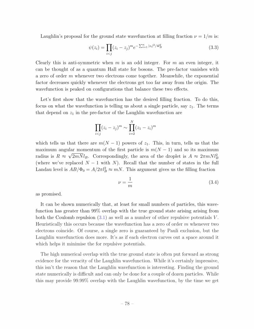


![Tunneling Experiments in the Fractional Quantum Hall E ect … · 2007-11-15 · The Quantum Hall e ect, and in particular the Fractional Quantum Hall e ect [4], have completely renewed](https://static.documents.pub/doc/80x56/5fa493c7a6ea3c531e644349/tunneling-experiments-in-the-fractional-quantum-hall-e-ect-2007-11-15-the-quantum.jpg)
