1 Composite Fermions And The Fractional Quantum Hall Effect: A Tutorial I. PRELIMINARIES The phenomenon of the fractional quantum Hall effect (FQHE) occurs when electrons are confined to two dimen- sions, cooled to near absolute zero temperature, and exposed to a strong magnetic field. It is one of the most important phenomena discovered during the last three decades. When one considers the scope and richness of phenomenology and the new physical principles required for its understanding, the FQHE rivals the phenomena of superconductivity and superfluidity. These lecture notes present an introduction to the essential aspects of the composite fermion (CF) theory of the FQHE, based on a set of lectures at a 2011 summer school in Bangalore, India, which, in turn, borrowed heavily from Ref. 1. The books 1–3 and review articles 4–9 listed at the end should be consulted for further details, more advanced topics, and references to the original papers. II. BACKGROUND This section contains some standard results. The missing derivations can be found in the literature. A. Definitions We collect here certain relevant units that will be useful below: flux quantum = φ 0 = hc e (1) magnetic length = ‘ = ~c eB 1/2 ≈ 25 p B[T] nm , (2) cyclotron energy = ~ω c = ~ eB m b c ≈ 20B[T] K , (3) Coulomb scale = V C ≡ e 2 ‘ ≈ 50 p B[T] K , (4) Zeeman splitting = E Z =2gμ B B · S = g 2 m b m e ~ω c ≈ 0.3B[T] K. (5) The last term in Eq. (2) quotes the magnetic length in nm. The last terms in Eqs. (3), (4), and (5) give the energy (in Kelvin) for parameters appropriate for GaAs (which has produced the best data so far). The magnetic field B[T] is in units of Tesla. The Zeeman splitting is defined as the energy required to flip a spin. B. Landau levels The Hamiltonian for a non-relativistic electron moving in two-dimensions in a perpendicular magnetic field is given by H = 1 2m b p + eA c 2 . (6) Here, e is defined to be a positive quantity, the electron’s charge being -e. For a uniform magnetic field, ∇ × A = B ˆ z . (7)
Transcript
1
Composite Fermions And The Fractional Quantum Hall Effect: A Tutorial
I. PRELIMINARIES
The phenomenon of the fractional quantum Hall effect (FQHE) occurs when electrons are confined to two dimen-sions, cooled to near absolute zero temperature, and exposed to a strong magnetic field. It is one of the most importantphenomena discovered during the last three decades. When one considers the scope and richness of phenomenologyand the new physical principles required for its understanding, the FQHE rivals the phenomena of superconductivityand superfluidity.
These lecture notes present an introduction to the essential aspects of the composite fermion (CF) theory of theFQHE, based on a set of lectures at a 2011 summer school in Bangalore, India, which, in turn, borrowed heavily fromRef. 1. The books1–3 and review articles4–9 listed at the end should be consulted for further details, more advancedtopics, and references to the original papers.
II. BACKGROUND
This section contains some standard results. The missing derivations can be found in the literature.
A. Definitions
We collect here certain relevant units that will be useful below:
flux quantum = φ0 =hc
e(1)
magnetic length = ` =(
~ceB
)1/2
≈ 25√B[T]
nm , (2)
cyclotron energy = ~ωc = ~eB
mbc≈ 20B[T] K , (3)
Coulomb scale = VC ≡ e2
ε`≈ 50
√B[T] K , (4)
Zeeman splitting = EZ = 2gµBB · S =g
2mb
me~ωc ≈ 0.3B[T] K. (5)
The last term in Eq. (2) quotes the magnetic length in nm. The last terms in Eqs. (3), (4), and (5) give the energy(in Kelvin) for parameters appropriate for GaAs (which has produced the best data so far). The magnetic field B[T]is in units of Tesla. The Zeeman splitting is defined as the energy required to flip a spin.
B. Landau levels
The Hamiltonian for a non-relativistic electron moving in two-dimensions in a perpendicular magnetic field is givenby
H =1
2mb
(p+
eA
c
)2
. (6)
Here, e is defined to be a positive quantity, the electron’s charge being −e. For a uniform magnetic field,
∇×A = Bz . (7)
2
The vector potentialA is a linear function of the spatial coordinates. It follows that H is a generalized two-dimensionalharmonic oscillator Hamiltonian which is quadratic in both the spatial coordinates and in the canonical momentump = −i~∇, and, therefore, can be diagonalized exactly.
We will use the symmetric gauge
A =B × r
2=B
2(−y, x, 0) . (8)
Taking the units of length as the magnetic length ` =√
~c/eB = 1, and the units of energy the cyclotron energy~ωc = ~eB/mbc = 1, and defining (notice the non-standard definitions)
z = x− iy = re−iθ, z = x+ iy = reiθ , (9)
the Hamiltonian becomes:
H =12
[−4
∂2
∂z∂z+
14zz − z ∂
∂z+ z
∂
∂z
]. (10)
We define the following sets of ladder operators:
b =1√2
(z
2+ 2
∂
∂z
)(11)
b† =1√2
(z
2− 2
∂
∂z
)(12)
a† =1√2
(z
2− 2
∂
∂z
)(13)
a =1√2
(z
2+ 2
∂
∂z
), (14)
which have the property that
[a, a†] = 1 , [b, b†] = 1 , (15)
and all the other commutators are zero. In terms of these operators the Hamiltonian can be written as
H = a†a+12. (16)
The Landau level (LL) index n is the eigenvalue of a†a. The z component of the angular momentum operator isdefined as
L = −i~ ∂
∂θ= −~(b†b− a†a) ≡ −~m (17)
with
m = −n,−n+ 1, · · · 0, 1, · · · (18)
in the nth Landau level. The application of b† increases m by one unit while preserving n, whereas a† simultaneouslyincreases n and decreases m by one unit.
The analogy to the Harmonic oscillator problem immediately gives the solution:
H|n,m〉 = En|n,m〉 (19)
En =(n+
12
)(20)
|n,m〉 =(b†)m+n√(m+ n)!
(a†)n√n!|0, 0〉 , (21)
3
The single particle orbital at the bottom of the two ladders defined by the two sets of raising and lowering operatorsis
〈r|0, 0〉 ≡ η0,0(r) =1√2π
e−14 zz , (22)
which satisfies
a|0, 0〉 = b|0, 0〉 = 0 . (23)
The single-particle states are especially simple in the lowest Landau level (n = 0):
η0,m = 〈r|0,m〉 =
(b†)m
√m!
η0,0 =zme−
14 zz√
2π2mm!, (24)
where we have used Eqs. (12) and (22). Aside from the ubiquitous Gaussian factor, a general state in the lowestLandau level is simply given by a polynomial of z. It does not involve any z. In other words, apart from the Gaussianfactor, the lowest Landau level (LLL) wave functions are analytic functions of z.
The LL degeneracy can be obtained by considering a region of radius R centered at the origin, and asking howmany states lie inside it. For the lowest Landau level, the eigenstate |0,m〉 has its weight located at the circle of radiusr =√
2m · `. Thus the largest value of m for which the state falls inside our circular region is given by m = R2/2`2,which is also the total number of eigenstates in the lowest Landau level that fall inside the disk (ignoring order onecorrections). Thus, the degeneracy per unit area is
degeneracy per unit area =B
φ0=
12π`2
(25)
which is the number of flux quanta penetrating the sample through a unit area.The filling factor is equal to the number of electrons per flux quantum, given by
ν =ρ
B/φ0= 2πl2ρ , (26)
where ρ is the 2D density of electrons. The filing factor is the nominal number of filled Landau levels.
C. Spherical geometry
F.D.M. Haldane introduced the spherical geometry for the study of the FQHE, wherein the two dimensional sheetcontaining electrons is wrapped around the surface of a sphere, and a perpendicular (radial) magnetic field is generatedby placing a Dirac magnetic monopole at the center of the sphere. The magnetic field
B =2Qφ0
4πR2r (27)
is produced by the vector potential
A = −~cQeR
cot θ φ . (28)
This geometry has played an important role in testing various theoretical conjectures. Two reasons for the popularityof this compact geometry are: First, it does not have edges, which makes it suitable for an investigation of the bulkproperties. Second, Landau levels have a finite degeneracy (for a finite magnetic field), which is useful in identifyingincompressible states for finite systems. In particular, filled Landau levels are unambiguously defined. (In the planargeometry, a finite number of electrons cannot fill a Landau level.) The spherical geometry has been instrumentalin establishing the validity of the theory of the FQHE, and provides the cleanest proofs for many properties. Wesummarize here some essential spherical facts, which will be very useful in the discussion below.
• The magnetic flux through the surface of the sphere, measured in units of the flux quantum, is quantized to bean integer for consistency, denoted by 2Q. The quantity Q, called the monopole strength, can be a positive ora negative integer or a half integer. The filling factor is defined by
ν = limN→∞
N
2Q. (29)
4
• The orbital angular momentum and its z component are good quantum numbers, denoted by l and m, respec-tively. Their allowed values are:
l = |Q|, |Q|+ 1, ... (30)
m = −l,−l + 1, ..., l . (31)
Each combination occurs precisely once. Note that the minimum value of l is |Q|, and l can be either an integeror a half-integer.
• Different angular momentum shells are the Landau levels in the spherical geometry. The degeneracy of eachLandau level is equal to the total number of m values, i.e., 2l + 1, increasing by two units for each successiveLandau level. In contrast to the planar geometry, the degeneracy is finite in the spherical geometry, due to itscompact nature. For the lowest Landau level, the degeneracy is 2|Q|+ 1; for the next it is 2|Q|+ 3; and so on.The lowest filled Landau level is obtained when N = 2|Q|+ 1. In general, the state with n filled Landau levelsis obtained when Q and N are related as
Q = ±N − n2
2n. (32)
• The single particle eigenstates are called monopole harmonics, denoted by YQlm(Ω), which are a generalizationof the familiar spherical harmonics. (The former reduces to the latter for Q = 0.) Ω represents the angularcoordinates θ and φ on the sphere. In the lowest Landau level, the monopole harmonics are given by
YQQm =[
2Q+ 14π
(2Q
Q−m)]1/2
(−1)Q−mvQ−muQ+m . (33)
with
u = cos(θ/2)eiφ/2, v = sin(θ/2)e−iφ/2. (34)
• The product of two single particle wave functions at Q and Q′ produces a wave function at Q + Q′. In otherwords, we have
YQlm(Ω)YQ′l′m′(Ω) =∑l”
Cl”YQ+Q′,l”,m+m′(Ω) . (35)
• Complex conjugation is equivalent to changing the sign of Q (or the magnetic field).
D. General LLL wave function
A many body wave function in the LLL has the form
Ψ = FA[zj] exp
[−1
4
∑i
|zi|2]
(36)
where FA[zj] is an antisymmetric polynomial of the zj . The LLL wave function has the property that the polynomialpart has no zj ’s, i.e., it is an analytic function. It is sometimes helpful to view FA[zj] as a polynomial in one ofthe coordinates, say z1, treating the other coordinates as variables. From the fundamental theorem of algebra, thenumber of zeroes is determined is equal to the degree of the polynomial, i.e. the largest exponent of z1. That is alsothe largest occupied orbital. Therefore, the number of zeroes is equal, modulo O(1) terms, to the number of fluxquanta penetrating the “sample.” The total number of zeroes of z1 is seen to be equal to N/ν, the angular momentumof the outermost occupied orbital. Furthermore, each zero is actually a vortex, in the sense that a closed loop of z1
around it produces a phase of 2π.The wave functions that involve the lowest n LLs contain at most (n − 1) factors of zj . Because FA is no longer
analytic, no simple statements can be made regarding the number of zeroes, which can now be vortices or anti-vortices.
5
E. Wave functions for filled Landau levels
For a general filling factor, for non-interacting electrons in the absence of disorder, the ground state is highlydegenerate, because electrons in the partially filled topmost Landau level can be arranged in a large number of ways.For an integral filling factor, ν = n, the ground state is unique, containing n fully occupied Landau levels. Its wavefunction is denoted by Φn. In the disk geometry, without a confinement potential there are an infinite number ofsingle particle orbitals; we will view a Landau level as “full” if all states inside a radius R are occupied.
The wave functions of filled Landau levels (in which all states inside a disk of some radius are filled) are uniquelydetermined; these are Slater determinants formed from the occupied single particle orbitals. The wave function of thelowest filled Landau level, Φ1 is given by (apart from a normalization factor):
Φ1 =
∣∣∣∣∣∣∣∣∣1 1 1 . .z1 z2 z3 . .z2
1 z22 z2
3 . .. . . . .. . . . .
∣∣∣∣∣∣∣∣∣ exp
[−1
4
∑i
|zi|2]
(37)
This is the so-called Vandermonde determinant, which has a particularly simple form:
Φ1 =∏j<k
(zj − zk) exp
[−1
4
∑i
|zi|2]
. (38)
F. Integer quantum Hall effect
When plotted as a function of the magnetic field B, the Hall resistance exhibits numerous plateaus. On any givenplateau, RH is precisely quantized at values given by
RH =h
ne2, (39)
where n is an integer. This phenomenon, discovered by Klaus von Klitzing, is referred to as the “integral quantumHall effect.” The RH = h/ne2 plateau occurs in the vicinity of ν ≡ Be/ρhc = n, where ν is the “filling factor,” i.e.,the number of filled Landau levels. In the plateau region, the longitudinal resistance exhibits an Arrhenius behavior:
Rxx ∼ exp(− ∆
2kBT
). (40)
This gives an energy scale ∆, which is interpreted as a gap in the excitation spectrum. Rxx vanishes in the limitT → 0, indicating dissipationless transport.
It is customary at first to neglect the Coulomb interaction in the treatment of the integral quantum Hall effect(IQHE). In general, the ground state at a non-integer filling factor is highly degenerate, because all arrangements ofelectrons in the topmost partially occupied LL have the same energy. However, unique ground state solutions areobtained at integer fillings. These are separated from excited states by a gap equal to the cyclotron energy. In otherwords, the system is incompressible. Including Coulomb interaction does not change this physics in the limit of largegaps.
R. B. Laughlin explained that the IQHE requires two ingredients: (i) the presence of a gap in a pure system atν = n, and (ii) weak disorder. The latter, which is always present in experiment, produces a reservoir of localizedstates in the gap, needed for the establishment of quantized plateaus.
6
Exercises
♣ Confirm that the eigenstates for magnetic field pointing in the −z direction are complex conjugates of the abovewave functions.♣ Show that the polynomial part of the single particle wave function (i.e. the factor multiplying the gaussian) ofthe nth LL involve at most n powers of z.♣ Obtain the second LL wave function |1,m〉.♣ Derive Eq. 38.♣ Show that the wave function of a lowest filled LL with a hole in the m = 0 state is given by
Φhole1 =
∏j
zj
Φ1 (41)
♣ Show that the wave function of a lowest filled LL with an additional electron in the second LL in the m = −1state (smallest angular momentum in the second LL) is given by
Φparticle1 =
N∑i=1
′∏j
(zi − zj)−1
zi Φ1 (42)
where the prime denotes the condition j 6= i.♣ Show that the wave function for two filled LLs is given by
Φ2 =
∣∣∣∣∣∣∣∣∣∣∣∣∣∣∣∣∣∣∣∣∣∣∣
1 1 1 . .z1 z2 z3 . .z2
1 z22 z2
3 . .. . . . .. . . . .
zN/2−11 z
N/2−12 z
N/2−13 . .
z1 z2 z3 . .z1z1 z2z2 z3z3 . .z1z
21 z2z
22 z3z
23 . .
. . . . .
. . . . .
z1zN/2−11 z2z
N/2−12 z3z
N/2−13 . .
∣∣∣∣∣∣∣∣∣∣∣∣∣∣∣∣∣∣∣∣∣∣∣
exp
[−1
4
∑i
|zi|2]. (43)
♣ Show that
φη(r) =1√2π
exp[
12ηz − 1
4|z|2 − 1
4|η|2]
(44)
is a coherent state, i.e. is an eigenstate of the angular momentum lowering operator b. Show that it represents agaussianly localized wave packet at η. Also show, using latter operators, that the coherent state in the nth LL is givenby
φ(n)η (r) ∼ (z − η)n exp
[12ηz − 1
4|z|2 − 1
4|η|2]. (45)
♣ Obtain the solution for an electron in a parabolic confinement potential in the presence of a magnetic field
H =1
2mb
(p+
e
cA)2
+12mbω
20(x2 + y2) (46)
where ω0 is a measure of the strength of the confinement. The solutions are known as Fock-Darwin levels.♣ Show that the in the spherical geometry, the wave function of the lowest filled LL is given by
Φ1 =∏j<k
(ujvk − vjuk) (47)
7
♣ Write the explicit wave function Φhole1 in the spherical geometry by leaving vacant the single particle orbital
centered at the north pole.♣ Confirm Eq. 35 for the product of two LLL wave functions at different flux values.♣ Show that
L+ = −u ∂∂v, L− = −v ∂
∂u, Lz =
12
(u∂
∂u− v ∂
∂v
), (48)
satisfy the standard angular momentum algebra, and produce the expected values when applied on YQQm.
8
III. THE FQHE PROBLEM
A. Phenomenology
The phenomenon of the FQHE, discovered by D.C. Tsui, H.L. Stormer and A.C. Gossard, refers to the observationof plateaus in the Hall resistance where it is quantized at
RH =h
fe2, (49)
where f is a fraction. The plateau characterized by the fraction f is centered at the filling factor ν = f . As inIQHE, the longitudinal resistance exhibits activated behavior in the plateau region, vanishing exponentially as thetemperature goes to zero, indicating the presence of a gap in the spectrum.
A great many experimental facts have been established. Beginning with 1/3, more than 70 fractions have beenobserved, to date, in the lowest Landau level, and ∼ 15 in the second Landau level. The number of FQHE statesis greater than the number of observed fractions, because states with many different spin polarizations have beenobserved at several fractions. One can list the observed fractions, but that will not be useful at this point. We willsee that the these fractions fall into a neat order once we understand their origin. (The situation can be likenedto organizing the atoms into the periodic table, which encapsulates deep connections between classes of atoms.) Inaddition to the fractionally quantized Hall resistance, many other properties have been measured, such as: excitationgaps; spin polarizations and transitions between differently spin polarized states as a function of the Zeeman energy;collective mode dispersions of neutral excitations with and without spin reversal; finite wave vector conductivity; andso on.
B. Questions for theory
We will neglect disorder in what follows and assume that, as in IQHE, the presence of a gap at a fractional fillingfactor ν = f for an ideal, disorder-free system, leads to a plateau quantized at RH = h/fe2 with the help of disorderinduced localization. The model of non-interacting electrons results in gaps only at integer fillings. We must thereforenow deal with the problem of interacting electrons in a strong magnetic field. The gap at fractional fillings mustoriginate from a collective behavior of the electron system.
The most important question that a candidate theory must address is: What is the mechanism of the FQHE? Theextensive phenomenology imposes stringent constraints on theory. Specifically, a candidate theory must explain: Whydo gaps open in a partially filled Landau level? Whey do fractions appear not in isolation but in certain sequences,such as f = n/(2n + 1) = 1/3, 2/5, 3/7, 4/9, 5/11, · · · ? What determines the order of stability of the fractions?(Order of stability refers to the fact that as samples are made purer and temperature is lowered, the fractions appearin certain order.) What different spin polarizations are possible at various fractions? Why does FQHE prominentlyoccur at certain odd-denominator fractions? Why is FQHE absent at ν = 1/2? What is the physics of the state atν = 1/2? Why does FQHE occur at 5/2? Why is FQHE much less prominent in the second Landau level comparedto that in the lowest Landau level?
In addition to the qualitative facts, we would like a candidate theory to provide a quantitative account of thephenomenon. It should be able to calculate gaps, collective mode dispersions, phase diagram of the spin polarization,and various response functions.
C. A nonperturbative many-body problem
The Schrodinger equation for interacting electrons in a magnetic field is given by
HΨ = EΨ , (50)
where
H =∑j
12mb
[~i∇j +
e
cA(rj)
]2
+e2
ε
∑j<k
1|rj − rk| +
∑j
U(rj) + gµB · S . (51)
9
U(r) is a one-body potential incorporating the effects of the uniform positive background and disorder, and the lastterm is the Zeeman energy. We will consider the limit of large magnetic fields such that
e2/ε`
~ωc=
e2/ε`
EZeeman= 0 (52)
In this limit all electrons have the same spin and occupy the LLL; their kinetic and Zeeman energies are constant,which we drop. We also forget about disorder, and suppress the background term. In units of the Coulomb energye2/ε`, the Hamiltonian becomes (with ` = 1)
H =∑j<k
1|rj − rk| (lowest Landau level) , (53)
which is to be solved in the LLL subspace. We refer to this as the “ideal” limit, because in this limit many parametersthat are not relevant to the FQHE physics drop out. In particular, none of the answers in the ideal limit may dependon the electron band mass, which is not a parameter of the ideal Hamiltonian; the energies of the ideal Hamiltonianwill depend only on the Coulomb scale VC.
Do not let the simplicity of H in Eq. 53 deceive you. This Hamiltonian actually shows that the FQHE problem isa nontrivial one, because it contains no small parameter – in fact, the ideal FQHE Hamiltonian has no parameters,period. To describe a system of interacting electrons we usually begin with a reference state, namely the exact groundstate of a suitably chosen H0. For example, Landau’s Fermi liquid theory treats interaction perturbatively aroundthe non-interacting Fermi sea, while the BCS theory finds an instability of the non-interacting Fermi sea state due toa weak attractive interaction. In the case of the FQHE, there is no H0. Switching off the interaction does not providea unique ground state but an exponentially large number of degenerate ground states. The ground state degeneracyis (
N/ν
N
), (54)
which is equal to the number of distinct arrangements of N electrons in N/ν single particle orbitals. This is of coursea very large number.
Experiments are telling us that when the Coulomb interaction is switched on, the exponentially large degeneracy iscompletely eliminated at some special filling factors to produce a gapped system with a non-degenerate ground statethat is some linear combination of the
(N/νN
)basis states. The effect of interaction is fundamentally non-perturbative,
because the opening of the gap is not related to the strength of the Coulomb interaction, which only sets the energyscale – an arbitrarily weak Coulomb interaction (as can be arranged by taking a very large dielectric constant ε) willopen a gap.
What physical mechanism underlying this drastic reorganization of the low energy behavior? How does it lead todramatic phenomena? What else does it produce?
10
IV. LAUGHLIN’S THEORY OF ν = 1/m STATE
Laughlin proposed the following elegant wave function for the correlated ground state at ν = 1/m:
Ψ1/m =∏j<k
(zj − zk)m exp
[−1
4
∑i
|zi|2]
. (55)
The exponent m must be an odd integer to satisfy the Pauli principle. Laughlin’s wave function was motivated by theJastrow ansatz used previously in the studies of helium superfluidity, and has been confirmed in exact diagonalizationstudies (results shown below). In addition to writing the wave function in Eq. 55, Laughlin also wrote an ansatzwave function for the quasihole excitations as a vortex in the wave function. He developed a mapping into a 2D onecomponent plasma, using which he showed that the wave function in Eq. 55 implies a uniform charge density withfilling factor 1/m, and that the quasiholes accumulate a fraction 1/m of the electron charge. It was subsequentlyshown by Arovas, Schrieffer and Wilczek that the quasiholes also acquire a fractional Berry phase when they windaround one another, i.e. obey fractional braid statistics.
If no other fractions had been discovered, then this article would end here. However, a great many fractions wereobserved subsequent to Laughlin’s work, a large majority of which do not fit into Laughlin’s theory.
What follows below is the CF theory of the FQHE, which was originally motivated by the analogy between theFQHE and the IQHE. It introduces a new kind of particles, called “composite fermions.” Composite fermions arepostulated to be the fundamental building blocks with which all FQHE states and their excitations are constructed,just as electrons are the fundamental building blocks for the IQHE states and their excitations. The CF theoryexplains the prominent FQHE as the IQHE of composite fermions, obtaining whole sequences of fractions at once.We will see that with the CF theory, the essential phenomenology of the FQHE can be understood without writingany wave functions. However, the CF physics also naturally suggests wave functions for all FQHE states and theirexcitations, which have been shown to be very accurate and allow quantitative calculations that can be comparedto laboratory and computer experiments. Laughlin’s wave function is recovered for ν = 1/m, but is seen to be apart of a larger structure and is understood as ν = 1 IQHE of composite fermions. Composite fermions also havemanifestations outside of the FQHE. The CF theory allows a general derivation of fractional charge and fractionalbraid statistics of the localized excitations.
We therefore defer the discussion of fractional charge and fractional braid statistics to a later stage, where we derivethem by methods that are applicable to all FQHE states, which we find to be conceptually more satisfying. The readerinterested in Laughlin’s motivation for writing the wave function in Eq. 55 and its mapping into a one componentclassical plasma is asked to consult the literature.
11
V. COMPOSITE FERMION THEORY
The CF theory begins with the anticipation that the FQHE and the IQHE are related and can be unified. Ex-perimentally, there is no qualitative distinction between the observations of different plateaus, be they integral orfractional, and therefore it does not seem unreasonable to expect that their physics might be similar. To be sure, theyall arise from the presence of a gap, but we are looking for a deeper connection.
A unification of the FQHE and the IQHE would imply that the FQHE be understood as the IQHE of certainemergent fermions. The search for a unified theory thus leads us to suspect the formation of some weakly interactingfermions. If such fermions can be identified, they will form the basis for exploring the detailed properties of the manybody state, because weakly interacting particles are what we understand best – perhaps the only thing we reallyunderstand. The emergent fermions of the FQHE state are obviously not electrons, because electrons exhibit only theintegral plateaus. What are they, then?
These fermions are called composite fermions. We begin by defining composite fermions:
a composite fermion = an electron + an even number of quantized vortices (56)
The vortex, by definition, is an object that produces a phase of 2π for a closed loop around it. The microscopicmeaning of this bound state is seen below. A less accurate but more pictorial way of defining a composite fermion is
a composite fermion = an electron + an even number of flux quanta (57)
where the vortex is modeled as a flux quantum φ0, which also has the property that a closed loop around it producesan Aharonov Bohm phase of precisely 2π. Care must be exercised not to take the second definition literally; no realfluxes are bound to electrons. The composite fermions are depicted as electrons with vertical arrows attached to them,each arrow representing a quantized vortex (or a flux quantum).
We note that the bound state of a fermion and a fraction of φ0 was used as a model for “anyon” had been introducedby J. M. Leinaas, J. Myrheim and F. Wilczek. The braid statistics depends on the value of the bound flux; bindingof an even number of flux quanta to fermions gives fermions, but with extra windings. A BEC-like description of theLaughlin 1/m state had been developed by Girvin and MacDonald, Zhang, Hansson and Kivelson, and Read in termsof electrons bound to an odd number of flux quanta, which satisfy bosonic statistics.
A. Accessing FQHE from IQHE through composite fermionization
The motivation for the above definition comes from the following mean field theory that seeks to obtain FQHEstates by “composite fermionizing” the IQHE states. I quote here from Ref. 1:
Step I: Let us consider non-interacting electrons at ν∗ = n. The many-particle energy spectrum is shown in theleft panel of Fig. (1). The ground state has n full Landau levels, shown schematically in the left column of Fig. (4 a)for ν∗ = 3. The lowest energy excited state is a particle-hole pair, or an exciton, shown in the left column of Fig. (2d). These diagrams have precise wave functions associated with them. We denote the magnetic field by B∗, whichcan be either positive or negative. It is related to the filling factor by ν∗ = ρφ0/|B∗| = n.
ch!*"
ener
gy
quantum number
ener
gy
#"
quantum number
FIG. 1: Left: The general structure of the energy spectrum of the many-body system at an integral filling, ν∗ = n. The x-axislabel is a convenient quantum number. The CF mean-field theory predicts that the low-energy spectrum at fractional fillingsν = n/(2pn ± 1) has similar structure, except that the states at ν are quasi-degenerate and the cyclotron gap evolves into aninteraction gap ∆.
The long range rigidity in the system at an integral filling factor (manifested by the presence of the gap) is causedsolely by the Fermi statistics. Thinking in the standard Feynman path-integral language is useful. The partition
12
FIG. 2: Panel (a) on the left shows the ground state at ν∗ = 3 with three filled LLs. The panels (b), (c) and (d) on the leftshow a particle, a hole, and a particle-hole excitations. The panels on the right schematically demonstrate the state obtainedafter the mean field theory, interpreted as the ground state (a) and the CF-quasiparticle, CF-quasihole and CF-quasiparticlequasihole excitations (b, c, and d, respectively.) Horizontal lines in the left column depict Landau levels of electrons, and thoseon right depict Λ levels of composite fermions; the dots are electrons and the dots adorned with two arrows represent compositefermions. The CF diagrams on the right are a pictorial representation of precise microscopic wave functions discussed in thetext.
function gets contributions from all closed paths in the configuration space for which the initial and the final positionsof electrons are identical, although the paths may involve fermion exchanges. Some examples are: a path in whichone electron moves in a loop while others are held fixed; or a cooperative ring exchange path in which the closedloop involves many electrons, with each electron moving to the position earlier occupied by the next one. Thephase associated with each closed path has two contributions: the Aharonov-Bohm phase which depends on the fluxenclosed by the loop; and the statistical phase, which is +1 or −1, depending on whether the final state is related tothe initial one by an even or an odd number of pairwise electron exchanges. The incompressibility at integral fillingsis presumably caused by some special correlations built in the phase factors of various paths. These correlations arenot easily identifiable in the path integral language, but we know they are present.
Step II: Now we attach to each electron a massless, infinitely thin, massless magnetic solenoid carrying 2p fluxquanta pointing in +z direction. This converts electrons into composite fermions. The flux added in this manner isunobservable, because it does not alter the phase factors associated with any closed Feynman paths. The excess ordeficit of an integral number of flux quanta through any closed path is physically unobservable, and the fermionicnature of particles guarantees that the phase factors of paths involving particle exchanges also remain intact. Inother words, the new problem defined in terms of composite fermions is identical to the original problem of non-interacting electrons at B∗. We have thus transformed an incompressible state of electrons into an incompressiblestate of composite fermions.
Step III. This exact reformulation prepares the problem for a mean-field approximation that was not available inthe original language. Let us adiabatically (i.e., slowly compared to ~/∆, where ∆ is the gap) spread the flux attached
13
to each electron until it becomes a part of the uniform magnetic field. (Because the initial state has a uniform electrondensity, the additional flux, tied to the density, produces a uniform magnetic field.) At the end, we obtain particlesmoving in an enhanced magnetic field B, given by
B = B∗ + 2pρφ0 . (58)
The relation |B∗| = ρφ0/n implies that B is always positive (pointing in the +z direction). The corresponding fillingfactor is given by
ν =n
2pn± 1, (59)
which follows from the relations ν = ρφ0/B and ν∗ = n = ρφ0/|B∗|. The + (−) sign in the denominator correspondsto B∗ pointing in the +z (−z) direction.
Let us now make the crucial assumption that the gap does not close during the flux smearing process, i.e., thereis no phase transition. To be sure, quantitative changes will occur. The gap and the wave functions will undergo acomplex evolution. (Recall that the IQHE gap is equal to the cyclotron energy, but the FQHE gap may not dependon the electron band mass; the flux spreading will not simply renormalize the value of the gap, but will have tochange its energy scale itself.) Nonetheless, if our assumption is correct, then Fig. (1) also represents, qualitatively,the spectrum at B.
The absence of a phase transition is an assumption that remains to be verified, and will surely not be valid for alln and p. If it is valid for some parameters, however, then the above construction gives a possible way of seeing howa gap can result at the fractions of Eq. (59). Three remarkable features already provide a strong hint that we are onthe right track: these fractions are precisely the observed fractions; they have odd-denominators; and we naturallyobtain sequences of fractions.
FIG. 3: CF mean field construction for deriving FQHE from IQHE. We begin with an IQHE state (a); attach to each electrontwo magnetic flux quanta to convert it into a composite fermion (b); and spread out the attached flux to obtain electrons in ahigher magnetic field, which is a FQHE state (c).
The three steps are depicted schematically in Fig. (3). The net effect, in a manner of speaking, is that each electronhas absorbed 2p flux quanta from the external magnetic field to transform into a composite fermion. Compositefermions experience the residual magnetic field B∗.
This can be generalized to arbitrary filling factors. For a general ν∗ we have a band of degenerate ground states fornon-interacting electrons. Proceeding as above, we first attach flux quanta to electrons to convert them into compositefermions, and then delocalize the flux to obtain electrons in magnetic field B = B∗ + 2pρφ0. If there are no levelcrossings, the mean field theory now predicts a quasi-degenerate band of ground states at B that has a one-to-onecorrespondence with the ground state band at ν∗.
B. Chern-Simons formulation of composite fermions
Chern-Simons approach has been used in the study of anyons (Laughlin); for a bosonic description of the 1/mground state (S.M. Girvin and A.H. MacDonald; S.C. Zhang, T.H. Hansson, and S.A. Kivelson); and for compositefermions (Jain; A. Lopez and E. Fradkin; B.I. Halperin, P.A. Lee and N. Read).
We started above with electrons at B∗, added 2p flux quanta to each electron, and then made a mean-field approx-imation to end up with fermions at B. In a time-reversed approach, we begin with electrons at B, attach 2p fluxquanta pointing in the direction opposite to B, and then perform a mean field approximation to cancel part of theexternal field, producing fermions at B∗ in the end. We consider the Schrodinger equation[
12mb
∑i
(pi +
e
cA(ri)
)2
+ V
]Ψ = EΨ , (60)
14
where V is the interaction. Through an exact singular gauge transformation defined by
Ψ =∏j<k
(zj − zk|zj − zk|
)2p
ΨCS , (61)
known as the Chern-Simons transformation, the eigenvalue problem can be expressed as
H ′ΨCS = EΨCS (62)
H ′ =
[1
2mb
∑i
(pi +
e
cA(ri)− e
ca(ri)
)2
+ V
](63)
a(ri) = 2pφ01
2π
′∑j
∇iθij , (64)
The vector potential −a amounts to attaching a point flux of strength −2pφ0 to each electron (exercise). TheLagrangian corresponding to this Hamiltonian contains the familiar Chern-Simons term ∼ εµναaµ∂νaα for 2 + 1dimensions; a is the Chern-Simons vector potential.
Further progress is not possible without making approximations. The usual approach is to make a “mean-field”approximation, which amounts to spreading the CS flux on each composite fermion into a uniform CS magnetic field,and assuming that, to zeroth order, the particles respond to the sum of CS and external fields. Formally, we write
A− a ≡ A∗ + δA , (65)
∇×A∗ = B∗z , (66)
B∗ = B − 2pρφ0 , (67)
where B∗ is the effective magnetic field experienced by composite fermions. The transformed Hamiltonian can nowbe written as:
H ′ =1
2mb
∑i
(pi +
e
cA∗(ri)
)2
+ V + V ′ = H ′0 + V + V ′ . (68)
V ′ contains terms proportional to δA. The solution to H ′0 is trivial, describing free fermions in an effective magneticfield B∗. We have thus decomposed the Hamiltonian into two parts: H ′0 can be solved exactly and the remainder,V + V ′, is to be treated perturbatively.
Let us neglect V + V ′ for a moment. Then, specializing to ν = n/(2pn+ 1), we get eigenfunctions
Ψαν (B) =
∏j<k
(zj − zk|zj − zk|
)2p
Φαn(B∗) , (69)
where Φαn are the solutions of non-interacting fermions at B∗ labeled by index α, with energies the same as those atB∗; in particular, the gap is given by
∆ = ~ω∗c = ~eB∗
mbc=
~(2pn+ 1)
eB
mbc, (70)
with B∗ = B/(2pn+1). This solution is far from the actual one. The actual energy gap is proportional to e2/ε` ∼ √B,the only energy scale in the LLL problem, and is independent of the electron mass, which is not a parameter of theLLL Hamiltonian. The mean-field wave function does not build favorable correlations between electrons, because itactually has the same probability amplitude as the uncorrelated IQHE wave function Φn. The wave function ΨMF alsoinvolves significant mixing with higher Landau levels, and at ν = 1/m, m odd, it does not reduce to Laughlin’s wavefunction. The perturbation theory program faces the formidable challenge, without a small parameter, of producingrepulsive correlations and of getting rid of the electron mass. It is not known what Feynman diagrams will accomplishthat. How do we proceed further, then?
B. I. Halperin, P. A. Lee and N. Read replace the electron band mass by an effective mass, which is to be determinedfrom other considerations and interpreted as the mass of composite fermions, and treat the above theory as an effectivemodel of composite fermions. We refer the reader to Refs. 6 and 7 for a review and references.
15
C. Wave functions for composite fermions
Further progress has been made by constructing trial wave functions for composite fermions based on the abovephysics. The problems mentioned above can be redressed to a large extent by boldly throwing away the denominatoron the right hand side of Eq. 69: the new wave function has good correlations, produces Laughlin’s wave function atν = 1/m, and resides predominantly in the LLL (as shown by explicit calculation). Because the denominator doesnot produce any Berry phases, the removal of the denominator does not alter the topological structure of the wavefunction; it simply converts the point flux quanta bound to electrons into vortices. In what follows, we will presentthis as our starting postulate, and then explore its various consequences.
The CF theory makes the postulate:
To minimize the interaction energy, each electron in the LLL captures an even number (2p)of quantum mechanical vortices to transform into entities called composite fermions, whichthemselves can be treated as weakly interacting fermions to a good first approximation.
In other words, the only essential role of interactions is to create composite fermions. As seen below, due to the Berryphases originating from the bound vortices, composite fermions experience an effective magnetic field
B∗ = B − 2pρφ0 (71)
They form Landau-like levels in the reduced magnetic field, called Λ levels, and their filling factor ν∗ = ρφ0/|B∗| isgiven by
ν =ν∗
2pν∗ ± 1(72)
The system of strongly interacting electrons in magnetic field B thus transforms into a system of weakly interactingcomposite fermions in an effective magnetic field B∗. The magnetic field B∗ and filling ν∗ are a direct consequenceof the formation of composite fermions.
Let us now define mathematically what various terms mean in the preceding paragraph. The meaning of electrons’capturing vortices implies the following form for the wave function:
ΨCF = Φ∏j<k
(zj − zk)2p (73)
where Φ is an antisymmetric wave function for electrons. The Jastrow factor∏j<k(zj − zk)2p ensures that each
particle sees 2p vortices on every other particle. The bound state of the electron and the vortices is interpreted as aparticle, called composite fermion.
Why would electrons capture vortices? It is easy to see that ΨCF is very efficient in keeping electrons away from oneanother, i.e. has good correlations in the presence of repulsive interactions. The probability of finding two electronsat a short distance r vanishes as r2(p+1) for ΨCF, which is much faster than the r2 behavior required by the Pauliprinciple. Of course, this is not a proof that binding vortices to electrons is the best way of minimizing interactions;we cannot rule out that nature would find a cleverer way. The validity of this ansatz must be ascertained by testingits consequences.
The meaning of “weakly interacting composite fermions” is that we take the wave function Φ to be the wavefunction of weakly- or non- interacting fermions, say at filling factor ±ν∗, where ± represents the direction of themagnetic field, and Φ−ν∗ ≡ [Φ+ν∗ ]∗ (complex conjugation of the wave function is equivalent to reversing the directionof the magnetic field). This explains the statement that the only role of interactions is to bind vortices to electronsto create composite fermions. The right hand side of Eq.73 has a dual interpretation: either as the wave function ofweakly interacting composite fermions at filling ν∗, or as a wave function of strongly correlated electrons at a fillingν (determined below).
An important conceptual ingredient is to allow Φ to occupy higher Landau levels (LLs), i.e., to allow the presenceof z’s in the wave function. Even though the wave function on the right hand side is not strictly in the LLL, explicitcalculations have shown that it is largely in the LLL, and is adequate for many qualitative purposes. However, becausethe limit of LLL, appropriate in the limit of very large magnetic fields, is a nice and convenient limit to consider,we would also like to have strictly LLL wave functions, which can be obtained by an “adiabatic continuation” ofthe above wave function to the LLL. We assume that can be accomplished by a straight LLL projection of the wavefunction, i.e. throwing away the part of this wave function that resides in higher Landau levels. We also assume that
16
this does not fully destroy the nice correlations built into the “unprojected” ΨCF of Eq. 73. This gives us the “final”expression for the wave function:
ΨCFν = PLLLΦ±ν∗
∏j<k
(zj − zk)2p (74)
with
Φ−ν∗ ≡ [Φν∗ ]∗ (75)
where PLLL represents LLL projection. We show below that ν is given by Eq. 72. Eq. 74 thus relates the wavefunctions of interacting electrons at ν, which we don’t know, with those of non-interacting fermions at ν∗, which wedo know. It is important to appreciate that ΨCF is not a single wave function, but gives wave functions for groundand excited states at all filling factors ν by analogy to the corresponding known states at ν∗. In particular, for theground state and the quasihole at ν = 1/m it reproduces Laughlin’s wave function (exercise). The mapping in Eq. 74assigns precise wave functions to the diagrams such as those shown in the right panels of Fig. 2 in terms of the knownwave functions in the left panels. Composite fermions are the building blocks of the FQHE in the same manner aselectrons are for the IQHE.
A remarkable feature of ΨCFν is that it gives the ground state at |ν∗| = n uniquely
ΨCFn
2pn±1= PLLLΦ±n
∏j<k
(zj − zk)2p (76)
with no adjustable parameters (e.g. Fig. 2a for ν∗ = 3). The same is true of the lowest neutral excitation, whosewave function is also fixed by symmetry for any given wave vector (Fig. 2d). The formation of composite fermions issuch a powerful constraint that once we assume the form of the wave function, the exponentially large degeneracy ofthe original problem is eliminated and no further variational freedom remains. Could one seriously expect these wavefunctions to capture the complex correlations of the FQHE state?
The relation between ν and ν∗ (Eq. 72), or the equivalent one between B and B∗ (Eq. 71), can be obtained inseveral ways. The simplest is power counting. Defining the size of the disk by the largest occupied orbital, which hasan angular momentum mmax, we have mmax + 1 flux quanta passing through the disk. The inverse filling factor isthen given by ν−1 = mmax/N , neglecting O(1) terms. For ΨCF
ν the largest occupied angular momentum is given by2p(N − 1)±N/ν∗, with the two terms on the right coming from the Jastrow factor and Φ±ν∗ . This gives the fillingfactor in Eq. 72. The magnetic field dependence comes through the magnetic length in the gaussian part of Φ±ν∗ . Ifwe keep the magnetic length fixed, the size of the QHE droplet increases upon multiplication by the Jastrow factorto produce a state with smaller density and thus a smaller filling factor.
Next we show that the effective magnetic field for composite fermions results because the Berry phases producedby the bound vortices partly cancel the Aharonov-Bohm phases due to the external magnetic field. For this purpose,we need to calculate the Berry phase of a vortex defined by the wave function
Ψη = NR∏j
(zj − η)Ψ , (77)
where Ψ is the wave function for the incompressible ground state in question and η = Re−iθ is the location of thevortex. Electrons avoid the point η, creating a hole there, which has a positive charge relative to the incompressiblestate. The normalization factor NR depends on the amplitude of η, but can be chosen to be independent of the angleθ. Let us now take η in a circular loop of radius R by slowly varying θ from 0 to 2π while holding R constant. (Weare treating η as a parameter in the Hamiltonian, which could be an impurity potential located at η that binds the
17
vortex.) Following Arovas, Schrieffer and Wilczek, the Berry phase associated with this path is given by
γ =∮
dt⟨
Ψη|i ddt
Ψη
⟩=∮
dθ⟨
Ψη|i ddθ
Ψη
⟩=∮
dθ(−i)dηdθ
⟨Ψη|
∑j
1zj − η |Ψη
⟩
=∮
(−i)dη∫
d2r1
z − η 〈Ψη|ρ(r)|Ψη〉
= 2π∫r<R
d2rρη(r)
= 2πNenc . (78)
In the above, we have used: ρ(r) =∑j δ
(2)(rj − r), ρη(r) = 〈Ψη|ρ(r)|Ψη〉, and Nenc is the number of particles insidethe closed loop. (Because of the definition z = x − iy, the residue for a contour integral differs from the usual bya sign.) The Berry phase of a vortex thus simply counts the number of particles inside the loop, with each particlecontributing 2π.
The net phase associated with a closed loop traversed by a composite fermion enclosing an area A is given by
Φ∗ = −2π(BA
φ0− 2pNenc
)(79)
where the first term is the Aharanov-Bohm phase of the electron and the second term is the Berry phase of the 2pvortices bound to the composite fermions. For uniform density states, we replace Nenc in Eq. 79 by its averagevalue ρA, where ρ is the electron or the CF density (this is a mean field approximation), and equate the entire phaseto the AB phase −2πB∗A/φ0 due to an effective magnetic field B∗. That produces the relation Eq. 71. We havederived this relation for the unprojected wave functions, but it should carry over to the projected wave function ifour assumption of adiabatic continuity is valid; direct numerical calculation of the Berry phase have confirmed Eq.79 for the projected wave functions.
It should be noted that the term vortex here is being used in a different sense than in a superconductor. For thelatter, it is the order parameter field that supports a vortex, which has associated with it circulating currents thatproduce a localized magnetic flux of hc/2e. For composite fermions there is no order parameter; the vortex structurebelongs to the the microscopic wave function, and has no magnetic flux or circulating currents associated with it.Also, the partial cancellation of the external magnetic field is not caused by an induced current (as for Meissner effectin a superconductor), but by induced Berry phases, and has a purely quantum mechanical origin. The cancellation isinternal to composite fermions. An external magnetometer will assess the full applied magnetic field. The only wayto measure the effective magnetic field is to use composite fermions themselves for the measurement.
D. Composite fermions on a sphere
We construct the wave function ΦQ∗ of non-interacting electrons at an effective flux Q∗, and multiply by a Jastrowfactor to obtain the wave function of composite fermions. The Jastrow factor of the planer geometry translates into∏
j<k
(zj − zk)2p →∏j<k
(ujvk − vjuk)2p = Φ2p1 (80)
where Φ1 is the wave function of the lowest filled LL. With LLL projection, this produces
ΨCFQ = PLLLΦQ∗
∏j<k
(ujvk − vjuk)2p = PLLLΦQ∗ Φ2p1 (81)
As noted earlier, the monopole strength of the product is the sum of monopole strengths. The monopole strength forΦ1 is Q1 = (N − 1)/2, because the LLL degeneracy here is 2Q1 + 1 = N , which gives
Q∗ = Q− p(N − 1) (82)
18
This equation is the spherical analog of Eq. 71: B∗ = B−2pρφ0. With ν = limN→∞N/2Q and ν∗ = limN→∞N/2|Q∗|,this relation reduces to Eq. 72 in the thermodynamic limit.
As in the planer geometry, we can construct wave functions for ground states as well as excitations. In the sphericalgeometry the exact many particle eigenstates are angular momentum multiplets. A nice property of Eq. 81 is that itpreserves the angular momentum quantum numbers in going from Q∗ to Q.
Proof: To see this, let us assume that ΦQ∗ is an eigenstate of the total angular momentum operators L2 and Lzwith eigenvalues L(L+ 1) and M . Write
L2 = L2z +
12
(L2+ + L2
−) (83)
where L+ = Lx + iLy and L− = Lx − iLy. The wave function Φ1 has L = 0, so it satisfies
LzΦ1 = L+Φ1 = L−Φ1 = 0 . (84)
Noting that all Lz, L+, and L− involve at most first order derivatives, we can commute them through the factor Φ1.Thus,
LzΦ21ΦQ∗ = Φ2
1LzΦQ∗ = MΦ21ΦQ∗ (85)
L2Φ21ΦQ∗ = Φ2
1L2ΦQ∗ = L(L+ 1)Φ2
1ΦQ∗ (86)
That the angular momentum is not altered upon projection into the lowest Landau level is seen most straightforwardlyby writing the projection operator, following Rezayi and MacDonald, as
PLLL =N∏i=1
PiLLL, PiLLL =∞∏
l=Q+1
l(l + 1)−L2i
l(l + 1)−Q(Q+ 1)(87)
where L2i is the angular momentum operator for the ith electron. That PLLL indeed is the projection operator is
seen by noting that PiLLL produces a zero when applied to any single particle state in a higher Landau level, and onewhen applied to any state in the lowest Landau level. Given that the total angular momentum operators L2 and Lzcommute with the L2
i of an individual electron, they also commute with the projection operator PLLL.The state with an integer number of filled ΛLs has L = 0, i.e. is invariant under rotation. Rotational invariance
in the spherical geometry is equivalent to translational invariance in the planar geometry. This implies, in particular,that the state ΨCF with L = 0 has uniform density. (This is one example of how the spherical geometry makes manyproperties essentially obvious; the demonstration of uniform density for ΨCF in the planar geometry requires somework.)
E. LLL projection
The LLL projection is given by (Exercise)
PLLLe−14 zz zmzs = e−
14 zz
(2∂
∂z
)mzs (88)
In other words, to project a wave function into the LLL requires us to write it in a “normal ordered” form by bringingall zj ’s to the left of the zj ’s, and making the replacement
zj → 2∂
∂zj(89)
with the understanding that the derivatives do not act on the gaussian part. Eq. 88 can be proved by noting that byrotational symmetry the only LLL state into which the projection is nonzero is ηo,m−s and evaluating its coefficient byusing the orthonormality of the single particle orbitals. The LLL projected CF wave functions can thus be explicitlywritten as
ΨCFν = PLLLΦ±ν∗
∏j<k
(zj − zk)2p =: Φ±ν∗(zj → 2∂/∂zj) :∏j<k
(zj − zk)2p (90)
19
Here : : is the normal ordering symbol, and the derivatives do not act on the gaussian part. (This method forprojection is not practical for very large systems; there a slightly different prescription for obtaining LLL statesproves more useful, but that is a technicality we will not go into here.) The same prescription works for the projectionof an operator V (z, z):
PLLLV (z, z)PLLL ≡ Vp(z, z) =: V(z → 2
∂
∂z, z
): (91)
Analogous expressions can be obtained for LLL projection in the spherical geometry, which we will not show explicitlyhere.
F. Energetics: CF diagonalization
For the most interesting states, namely the ground states and low energy excitations at ν = n/(2pn± 1), the wavefunctions ΨCF are determined completely by symmetry (examples are given below). The predictions for the groundstate energy and the CF exciton dispersion are obtained by evaluating the expectation value of the Hamiltonian withrespect to these wave functions. Because these are strictly in the LLL, the kinetic energy part is the same for allstates at a given ν and the energy differences depend only on the Coulomb scale VC, as must be the case in the LLL.
In general, for ν∗ 6= n, the CF construction gives several states in the lowest energy band, which are treated ascorrelated basis functions. The CF spectrum is obtained by diagonalizing the Coulomb interaction in this basis. Thesimplification is that the dimension of the CF basis is exponentially small compared to that of the full LLL basis. Thecomplication is that the CF basis functions are rather complicated, and also not necessarily orthogonal. The evaluationof the CF spectrum requires what is known as “CF diagonalization,” which involves LLL projection, Gram-Schmidtorthogonalization, evaluation of the Hamiltonian matrix, and diagonalization. This can be done exactly for smallsystems. Efficient Monte Carlo methods have been developed for CF diagonalization for fairly large N , which givethe CF spectra and CF eigenstates with high precision. Through these methods the CF theory allows quantitativecalculations on rather large systems, involving up to 50-200 composite fermions depending on the filling factor, whichenables reliable estimates of the thermodynamic values for various gaps, dispersions, and phase transitions.
20
Exercises
♣ Show that the vector potential a = (φ/2π)∇θ produces a flux tube of strength φ at the origin, i.e. ∇×a = φδ(r).♣ Evaluate the Berry phase for the localized wave packet given in Eq. 44 for a circular loop and show that it isequal to the Aharonov-Bohm phase.♣ Show that the ground state wave function of one filled Λ level of composite fermions (ν∗ = 1) is identical toLaughlin’s wave function of Eq. 55 at ν = 1/(2p+ 1). No LLL projection is needed in this case.♣ We derived the wave functions for the hole and particle of ν = 1 state. Construct the corresponding wavefunctions for the CF-quasihole and the CF-quasiparticle at ν∗ = 1. Then go ahead and construct the wave functionsfor two CF-quasiholes and two CF-quasiparticles in the innermost angular momentum states.♣ Prove that V and Vp in Eq. 91 have identical matrix elements within the LLL, but when applied to a LLL state,Vp causes no mixing with higher LLs.♣ Show that xp and yp, the projected coordinates, obey the commutator
[xp, yp] = i`2 (92)
The LLL space is said to be non-commutative.♣ Prove Eq. 88 by two methods. (i) Noting that the projection is nonzero only for the LLL orbital with angularmomentum s−m, evaluate its coefficient by using completeness relation. (ii) Consider zmφ, where φ is an arbitrarylowest Landau level wave function. Express z in terms of ladder operators and show that the LLL projection produces(√
2b)mφ.
21
VI. EXPLANATION OF THE PROMINENT FQHE
FIG. 4: Schematic view of the electron ground state at ν∗ = n (left column). The columns on the right show the CF view ofthe ground states at ν = n/(2n+ 1), as ν∗ = n filled Λ levels of composite fermions.
Due to the formation of composite fermions, the LLL splits into Λ levels of composite fermions that are analogousto LLs of electrons in an effective magnetic field. Gapped states are obtained when the CF filling is integer, i.e. ν∗ = n(Fig. 4), which corresponds to the electron filling factors given by
ν =n
2pn± 1(93)
Within the LLL, we can equally well express the original problem in terms of holes by using the exact particle holesymmetry. Composite fermionization of holes produces hole filling factors of Eq. 93, which correspond to electronfilling factors given by
ν = 1− n
2pn± 1(94)
In other words:
FQHE of electrons = IQHE of composite fermions (95)
The understanding of the FQHE of electrons as the IQHE of composite fermions explains the following observations:
• Only odd denominator fractions are obtained.
• Fractions appear in sequences, because they are all derived from the sequence of integers.
• The fractions given by Eq. 93 are indeed the prominent fractions observed in experiments. For example, thedata in Fig. 5 show the sequences:
n
2n+ 1=
13,
25,
37,
49,
511, · · · (96)
n
2n− 1=
23,
35,
47,
59, · · · (97)
The fractions belonging to the sequences n/(4n + 1) and n/(4n − 1) are seen at higher magnetic fields, in therange 1/3 < ν ≤ 1/5. Fig. 7 shows all observed fractions that are understood as IQHE of composite fermions.
22
FIG. 5: The Hall and the longitudinal resistances, RH and R, respectively. The fractions associated with the plateaus (or theresistance minima) are indicated. Source: Willet et al. Phys. Rev. B 37, 8476(1988).
14_
12_
123465 2
3_
49_
35_
59_
37_4
7_
52_ 1
3_p
2p±1113_7
2_
415_
313_
417_
p4p±1
14_
12_
113_7
2_
415_
313_
417_
p4p±12
3_
49_
35_
59_
37_4
7_
52_ 1
3_p
2p±1
0 6 12 18Magnetic Field (T)
FIG. 6: Plotting FQHE data as a function of the effective magnetic field by shifting the magnetic field axis by 2ρφ0 demonstratesits similarity to the IQHE. Source: H.L. Stormer.
• The CF theory explains the similarity of the FQHE data, plotted as a function of the effective field, with theIQHE (see Fig. 6). Although obvious in retrospect, it had not been noticed prior to the CF theory. Thecomparisons show that just as transitions from one integral plateau to another occur as the Fermi level passesthrough LLs, so do transitions from one fraction to the next as the Fermi level crosses Λ levels.
• The exactness of the Hall quantization results because the number of vortices bound to composite fermions (2p)and the number of filled ΛLs (n) are both integers; consequently, the right hand side of f = n/(2pn± 1) is notsusceptible to continuous variations of parameters.
23
ν =n
2n + 1=
1
3,2
5,3
7,4
9,
5
11,
6
13,
7
15,
8
17,
9
19,10
21
ν =n
2n− 1=
2
3,3
5,4
7,5
9,
6
11,
7
13,
8
15,
9
17,10
19
ν = 2− n
2n− 1=
4
3,7
5,10
7,13
9,16
11,19
13,22
15
ν = 2− n
2n + 1=
5
3,8
5,11
7,14
9,17
11,20
13,23
15
ν =n
4n + 1=
1
5,2
9,
3
13,
4
17,
5
21,
6
25
ν = 1 +n
4n + 1=
6
5,11
9
ν = 1− n
4n + 1=
4
5,7
9,10
13
ν = 2− n
4n + 1=
9
5
ν =n
4n− 1=
2
7,
3
11,
4
15,
5
19,
6
23
ν = 1− n
4n− 1=
5
7,
8
11,11
15
ν = 1 +n
4n− 1=
9
7
ν = 2− n
4n− 1=
12
7
ν =n
6n + 1=
1
7,
2
13,
3
19
ν =n
6n− 1=
2
11,
3
17
ν =n
8n + 1=
1
9,
2
17
ν =n
8n− 1=
2
15
1
FIG. 7: The observed fractions in the lowest Landau level (0 ≤ ν ≤ 2) that correspond to IQHE of composite fermions [Stormer,private communication]. Additionally, there exists evidence for 4/11, 5/13, 4/13, 7/11, 5/17, 6/17, and indications also for3/8 and 3/10 [Pan et al. (2003)], which are not explicable as IQHE of composite fermions. Many of the above fractions havebeen seen only in the longitudinal resistance Rxx; it is probable that the corresponding Hall plateaus will eventually be seenunder sufficiently improved experimental conditions. The fractions for composite fermions with vorticity 2p = 6 and 2p = 8appear only under somewhat elevated temperatures [Pan et al. (2002)], presumably above the melting temperature of thecrystal ground state. Source: H. L. Stormer, private communication; W. Pan, H. L. Stormer, D. C. Tsui, L. N. Pfeiffer, K. W.Baldwin, and K. W. West, Phys. Rev. Lett. 90, 016801 (2003).; W. Pan, H. L. Stormer, D. C. Tsui, L. N. Pfeiffer, K. W.Baldwin, and K. W. West, Phys. Rev. Lett. 88, 176802 (2002).
• It is tempting to model the system in terms of non-interacting composite fermions with an effective mass m∗.Then the CF cyclotron energy is given by
~ω∗c = ~eB∗
m∗c= ~
eB
(2pn± 1)m∗c≡ C
2pn± 1e2
ε`(98)
Here we have assumed filling factor ν = n/(2pn ± 1) for which B∗ = B/(2pn ± 1). We have also used thefact that the cyclotron energy must eventually be proportional to the Coulomb interaction, which requires thatm∗ ∼ √B. This is all based on several assumptions, but the theoretically obtained gaps do indeed appear tofollow this behavior. The experimental gaps behave as
∆ n2n±1
=C
2pn± 1e2
ε`− Γ (99)
where Γ is interpreted as the disorder induced broadening of the ΛLs. This provides an experimental determi-nation of the CF mass. The CF mass is roughly filling factor independent. This mass m∗ has no relation to the
24
electron band mass; it arises purely due to interactions. This also provides an insight into the extraordinarystability of FQHE along the sequences n/(2pn± 1), because the gaps decay very slowly with increasing n.
The FQHE and the IQHE are thus unified. We also now have a physical understanding of the origin of gaps in apartially filled Landau level: when composite fermions are formed, the LLL splits into Λ levels (ΛLs) of compositefermions, and incompressible states are obtained when an integral number of ΛLs are full.
25
VII. SPIN PHYSICS
In our discussion above we have considered fully spin-polarized states, as appropriate in the limit of very largeZeeman energies. Partially spin polarized or spin single FQHE states become possible at low Zeeman energies. Let usassume that composite fermions are formed even at low Zeeman splittings, and can be taken as nearly independentparticles. Their IQHE occurs at ν∗ = n = n↑+n↓, where n↑ and n↓ are the number of occupied spin-up and spin-downΛ levels. This corresponds to electron fillings
ν =n
2pn± 1=
n↑ + n↓2p(n↑ + n↓)± 1
. (100)
The spin polarization of the state is given by
γe =n↑ − n↓n↑ + n↓
, (101)
E z
(4,0) (3,1) (2,2)
FIG. 8: Schematic view of the evolution of the FQHE state at ν = 4/9 or 4/7, which maps into ν∗ = 4 filled Λ levels, as afunction of the Zeeman energy, EZ. The three different possible states are (n↑, n↓) = (4, 0), (3, 1), and (2, 2).
experimental confirmation
Kukushkin et al.
AlAs quantum wells
Park and Jain, 1998
Padmanabhan et al. Bishop et al.Du et al.
Du
Kukushkin
TheoryTheory
FIG. 9: Spin transitions are seen in transport by varying the Zeeman energy by tilting the field while keeping the perpendicularcomponent fixed (upper left) and by optical means (upper right). The upper middle plot shows transitions for a system withtwo valleys. The lower plots compare the measured positions of the transitions with that predicted by theory for spin transitions(lower left) and valley transitions (lower middle). Source: I. V. Kukushkin, K. v. Klitzing, and K. Eberl, Phys. Rev. Lett. 82,3665 (1999); R. R. Du, A. S. Yeh, H. L. Stormer, D. C. Tsui, L. N. Pfeiffer, and K. W. West, Phys. Rev. Lett. 75, 3926 (1995);Medini Padmanabhan, T. Gokmen, and M. Shayegan, Phys. Rev. B 80, 035423 (2009); N. C. Bishop, M. Padmanabhan, K.Vakili, Y. P. Shkolnikov, E. P. De Poortere, and M. Shayegan, Phys. Rev. Lett. 98, 266404 (2007); K. Park and J. K. Jain,Phys. Rev. Lett. 80, 4237 (1998).
Thus, the FQHE occurs at the same fractions as before (Eq. 93) but many states with different spin polarizationare possible at each fraction. The possible states for ν = 4/7 or 4/9 are illustrated in Fig. (8). As the Zeeman energyis lowered, the FQHE system undergoes magnetic phase transitions from one incompressible state to another.
26
Some typical examples are:
• The state at ν = 1/3, which corresponds to ν∗ = 1 filled Λ level, is always fully spin polarized, no matter howsmall the Zeeman energy. This physics is analogous to the spontaneous polarization of the ν = 1 state.
• The states at 2/3, 2/5 etc., which corresponds to ν∗ = 2 filled Λ levels, can be either spin singlet or fully spinpolarized. (Note that the fully spin polarized state at 2/3 can be understood in two ways: either as the holepartner of 1/3 or as ν∗ = 2 of composite fermions with reverse flux attachment. These two give same quantumnumbers and almost the same wave functions, and are thus equivalent. However, only the latter understandingbrings out the spin singlet state.)
• The states at 3/7, 3/5, etc., which correspond to ν∗ = 3 can be fully polarized or partially polarized (but notunpolarized).
• The states with even numerators can be spin singlet, whereas those with odd numerators will not have spinsinglet FQHE.
The Zeeman energy can be varied, for example, by application of an additional magnetic field parallel to the layer(i.e. by tilting the sample while holding the perpendicular component of the field fixed), which affects the Zeemanenergy but, to the lowest order, not the interaction energy. The above physics has been confirmed by transportand optical experiments, with some experiments shown in Fig. 9. Phase transitions have been observed and theZeeman splittings where they occur agree well with the theoretical predictions. The spin polarizations have also beenmeasured and agree with the expression in Eq. 101. Interestingly, the spin physics of the FQHE is richer than thatof the IQHE (in GaAs) because the Zeeman energy is very small compared to the electron cyclotron energy (thusproducing the state with the smallest spin polarization), but it is typically comparable to the FQHE gaps (interpretedas the cyclotron energy of composite fermions).
The results in this section also apply to experimentally observed FQHE in multivalley systems, such as the onein AlAs quantum wells, with the two valleys playing the role of the two spin components. These consideration canbe extended to situations where each electron has four components, e.g. graphene where the electron has two valleyindices (called K and K’ points) and two spin indices. See Fig. 9 for experiments on AlAs quantum wells.
27
VIII. HALF FILLED LANDAU LEVEL: THE DOG THAT DID NOT BARK
Magnetic focusing (Goldman; Smet)
Antidot resonances (Kang)SAW (Willett, 1993)
B*
B
Cyclotron radius
e
CF
Effective magnetic field B*
FIG. 10: A collection of some experiments that measure the CF Fermi sea through a measurement of the cyclotron orbit ofthe fundamental current carriers. Source: R. L. Willett, R. R. Ruel, K. W. West, and L. N. Pfeiffer, Phys. Rev. Lett. 71,3846 (1993); W. Kang, H. L. Stormer, L. N. Pfeiffer, K. W. Baldwin, and K. W. West, Phys. Rev. Lett. 71, 3850 (1993); V.J. Goldman, B. Su, and J. K. Jain, Phys. Rev. Lett. 72, 2065 (1994); J. H. Smet, D. Weiss, R. H. Blick, G. Lutjering, K. vonKlitzing, R. Fleischmann, R. Ketzmerick, T. Geisel, and G. Weimann, Phys. Rev. Lett. 77, 2272 (1996).
One of the mysteries had been the lack of FQHE at ν = 1/2, which is the simplest fraction. If composite fermionsare relevant at ν = 1/2, where B = 2pρφ0, they would experience no effective magnetic field, i.e. we have B∗ = 0.Halperin, Lee and Read made the proposal that composite fermions form a Fermi sea here:
1/2 filled LL = CF Fermi sea (102)
Because the Fermi sea has no gap, no FQHE may occur here insofar as the model of non-interacting composite fermionsis valid. Of course, one cannot rule out that the residual interaction between composite fermions may open a gap, butshould that happen, the resulting state is expected to be much weaker than the IQHE states of composite fermions.The absence of FQHE at ν = 1/2 down to the lowest available temperatures indicates that residual interactionsbetween composite fermions only cause perturbative corrections to a very good approximation.
The FQHE sequence n/(2n±1) terminates into 1/2 in the limit n→∞. The state with an infinite number of filledΛ levels is nothing but a Fermi sea of composite fermions, just as an infinite number of filled LLs is another name forthe Fermi sea of electrons. The same conclusion is reached by noting that the effective magnetic field B∗ = B − 2ρφ0
vanishes at ν = 1/2 because B = ρφ0/ν. The following observations confirm the CF Fermi sea1,4,8,9:
• The state remains compressible down to the currently lowest attainable temperatures.
• The current carrying objects execute semiclassical cyclotron orbits in the vicinity of ν = 1/2 that have beenmeasured in several experiments. The measured radius is consistent with
R∗c =~k∗FeB∗
, (103)
with k∗F =√
4πρ, as appropriate for a fully polarized CF Fermi sea. The radius is much larger than that of theorbit an electron would execute in the external magnetic field.
• Quantum oscillations, the telltale signature of a Fermi sea, have been observed, and are well described bystandard expressions developed for an ordinary Fermi sea.
• The temperature dependence of the spin polarization of the 1/2 state is consistent with that of a Fermi sea ofnon-interacting fermions.
28
IX. COMPUTER EXPERIMENTS
From a microscopic perspective, the CF theory makes detailed quantitative predictions about the low energy sectorof the energy spectrum of interacting electrons in the LLL. To summarize:
The CF theory predicts that the exact spectrum of interacting electrons contains a low energyband of states separated from the rest by a gap; further it predicts the quantum numbers,wave functions, and energies, for all states in this band, at all filling factors, by analogy to thelow energy band of noninteracting fermions at the corresponding effective filling factor.
This is best illustrated by taking two examples. The spherical geometry is the most convenient for this purpose.Example (i): Consider a system of N = 10 electrons at flux 2Q = 21. Here, in the absence of interactions we have(
2210
)degenerate ground states, which can be chosen as angular momentum eigenstates, with ML degenerate multiplets
at each allowed L. The structure of the Hilbert space is given by
As explained below, the CF theory predicts that with interactions the low energy part of the spectrum splits intomini bands of composite fermions with the structure:
(the reason why 1 is crossed out is explained below). According to Eq. 82, choosing 2p = 2, this system maps intoa system of weakly interacting fermions at Q∗ = 1.5. What do we know about this system? The LLL is an l = 3/2shell with 2l + 1 = 4 orbitals, the second LL is an l = 5/2 shell with 6 orbitals, the third LL is an l = 7/2 shell with8 orbitals, and so on. With 10 particles the ground state is non-degenerate, obtained by filling the lowest two LLs.(This state is thus a finite size representation of ν∗ = 2 of composite fermions, or ν = 2/5 of electrons.) Being a filledshell state, it has total orbital angular momentum L = 0. The lowest energy excited states are CF excitons, obtainedby promoting a fermion from the l = 5/2 shell to the l = 7/2 shell. The allowed angular momenta for the excitonthus are L = 1, 2, 3, 4, 5, 6, with a single multiplet at each of these values. Furthermore, we can write the explicitwave functions of these states at Q∗, from which we can construct ΨCF
Q for interacting electrons at Q. With the wavefunctions, the energies are obtained by taking expectation value of the Coulomb interaction; this requires some work,but is in principle straightforward.
Being a single state, the wave function ΦQ∗ is determined uniquely by group theory for the ground state or theexciton, and hence ΨCF
LLL has no dependence on the interaction either for these states. As mentioned above, thisremains the case for arbitrarily large N for systems that map into filled shells at the effective flux, which are the mostinteresting states, namely the incompressible states responsible for the FQHE.
Finally, a somewhat subtle point ought to be noted: some state at Q∗ might not produce a state at Q, becausethe wave function may be annihilated upon LLL projection. For the lowest energy band, no such annihilations areknown to occur; each state at Q∗ produces a state at Q. Such one-to-one correspondence between Q∗ and Q is lostfor higher bands, however (as it must, given that there are only a finite number of LLL states at Q but an infinitenumber of state at Q∗ where we allow all LLs). The first example is the L = 1 exciton state, which is annihilated byLLL projection.
Example (ii): Consider next a system of N = 8 electrons at 2Q = 18. Here, for non-interacting electrons we have
To see how this is arrived at, first notice that the system maps into 8 weakly interacting fermions at Q∗ = 2. TheLLL accommodates 2Q∗ + 1 = 5 fermions, which can be treated as inert. We are thus left with three fermions inthe angular momentum l = 3 shell, where they can occupy lz = −3,−2,−1, 0, 1, 2, 3 orbitals. The allowed L valuescan be obtained from elementary group theory. The simplest method is to list all distinct configurations for variousvalues of Lz consistent with the Pauli principle. This gives us 5, 4, 4, 3, 2, 1, 1 distinct configurations at Lz =0, 1,2, 3, 4, 5, 6, respectively. Noting that each L multiplet produces one state at Lz = −L,−L+ 1, · · ·L, we obtain theallowed L values quoted in Eq. 107. Again, the wave functions of these states can be constructed (no more than asingle state occurs at each L value at the effective flux 2Q∗, and therefore the wave function ΦQ∗ is determined at
29
0 2 4 6 8 10 12L
-0.442
-0.441
-0.440
-0.439
-0.438
-0.437
-0.436
-0.435
-0.434
E [
e2/!l]
N=12, 2Q=29
-0.45
-0.44
-0.43
-0.42
-0.41
31
42
101
111
168
175
227
230
277
-0.49
-0.48
-0.47
-0.46
-0.45
-0.44
52
83
179
212
304
328
416
8 8 21
22
35
33
0 3 6 9 12
-0.51
-0.50
-0.49
-0.48
-0.47
-0.46
L
127
263
493
621
952
744
1182
0 3 6 9 12
L
8 8 21
22
35
33
45
-0.46
-0.45
-0.44
-0.43
-0.42
-0.41
N=8, 2Q = 19
31
42
101
111
168
175
227
230
277
N=8, 2Q = 20
126
0 3 6 9 12-0.48
-0.47
-0.46
-0.45
-0.44
-0.43
L
N=8, 2Q = 17
12
10
32
30
51
48
0 3 6 9 12
L
N=8, 2Q = 18
13
17
42
75
111
70
91
FIG. 11: Top left: Comparison of exact spectra (dashes) and CF spectra (dots) for Coulomb interaction. Top two spectracorrespond to (N, 2Q) = (10, 27) and (8, 21); middle two spectra correspond to (N, 2Q) = (10, 21) and (8, 16); and bottomtwo spectra correspond to (N, 2Q) = (12, 23) and (9, 16). Source: Chapter 1 by J.K. Jain and R.K. Kamilla, in Ref. 2. Topright: Comparisons for larger systems at 1/3, 2/5 and 3/7. The dark dots are exact spectra and the light dots are CF spectra.Source: A. Wojs. Bottom left: Comparison for (N, 2Q) = (12, 29), which is a finite size representation of ν = 4/11; only the lowenergy part of the spectrum is shown. (Source: J.K. Jain, C.-C. Chang, G.-S. Jeon, and M.R. Peterson, Solid State Commun.127, 809 (2003).) Bottom right: Comparisons for several eight particle systems between 1/3 and 2/5 (Source: Chapter 1by J.K. Jain and R.K. Kamilla, in Ref. 2). The energies (per particle) are given in units of e2/εl. The spherical geometryis assumed, in which electrons move on the surface of a sphere in the presence of a radial magnetic field. The eigenstatesare organized according to their total orbital angular momentum L, which is a good quantum number in this geometry. TheHilbert space is restricted to the lowest Landau level. Only the very low energy part of the spectrum is shown; the number oflinearly independent multiplets in each L sector is shown at the top. With the exception of the labels of the top right panels,all energies shown are energies per particle and include interaction with the background.
each L uniquely from group theory alone) and their Coulomb energies evaluated by straightforward (albeit sometimescumbersome) methods.
We compare in this section results from two independent sets of calculations. (a) One calculation obtains the exactCoulomb spectra and exact Coulomb eigenstates of N interacting electrons at flux 2Q by a brute force numericaldiagonalization. (b) In the second calculation, we obtain the spectra predicted by the CF theory, again without makingany approximations. For this purpose, we enumerate all degenerate ground states and their quantum numbers (e.g.the orbital angular momentum) of free fermions at 2Q∗ = 2Q − 2(N − 1). The CF theory predicts that these arethe quantum numbers of the low energy states at 2Q. We then construct the CF wave functions according Eq. 74.When the wave function is uniquely determined, as is the case for the filled ΛL ground state at ν∗ = n and its CFexciton, all that we need to do is evaluate the expectation value of its Coulomb energy. In general, we perform aCF diagonalization to obtain the CF spectrum. Because both calculations are exact with no adjustable parameters,
30
FIG. 12: This figure shows a comparison between the energies predicted by the CF theory (dots) and the exact Coulombenergies (dashes), both obtained without any adjustable parameters. The spectra shown are for (a) 14 electrons exposed to39 flux quanta, (b) 16 electrons exposed to 36 flux quanta, and (c) 18 electrons exposed to 37 flux quanta; these are finitesize representations of the 1/3, 2/5 and 3/7 states. The dots show the Coulomb energies of the CF wave functions for theground states and the neutral excitations (the CF wave function for the 1/3 ground state at L = 0 coincides with Laughlin’swave function). The energies (per particle) are given in units of e2/εl, and include the interaction with the uniform positivelycharged background. The spherical geometry is assumed, in which electrons move on the surface of a sphere in the presence ofa radial magnetic field. The eigenstates are organized according to their total orbital angular momentum L, which is a goodquantum number in this geometry. The Hilbert space is restricted to the lowest Landau level. Only the very low energy partof the spectrum is shown; the number of linearly independent multiplets in each L sector is shown at the top. Source: A. C.Balram, A. Wojs, J. K. Jain, Phys. Rev. B 88, 205312 (2013), which also contains many comparisons for systems away fromthe special fractions n/(2n+ 1).
the comparisons are unbiased. (For ΨCF we can obtain the energy either exactly or by the Monte Carlo method forevaluating multi-dimensional integrals; the latter gives results as accurately as we please by running the computerlong enough, but we typically settle for four significant figure accuracy.)
We put the exact and the predicted spectra on the same plot in Figs. 11 and 12 for 18 different systems labeled by(N, 2Q). The following features can be noted:
• The exact many body spectrum indeed contains a low energy band of states. This low energy structure arisespurely due to interactions; all LLL states would be degenerate in the absence of interactions.
• The structure of the low-energy band depends on 2Q and N in a seemingly haphazard manner, but is seen tohave a one-to-one correspondence with that of noninteracting fermions at 2Q∗, as predicted by the CF theory.(These quantum numbers were worked out above in Sec. IX and are left for exercises.)
• The quantum numbers of the exciton band are also predicted correctly.
• The energies obtained from ΨCF are very accurate. They are typically within 0.1% of the exact energy for thesystems studied.
• The wave functions ΨCF have a near unity overlap with the corresponding exact eigenstates (Table I).
To assess the significance of these comparisons, we note that each eigenstate is a linear combination of a largenumber of basis functions, shown at the top of several panels, and therefore an agreement for even a single eigenstateis nontrivial, especially in view of the parameter-free nature of the theory. Figs. 11 and 12 show comparisons for∼150 eigenstates. The CF theory has been compared with exact results for a large number of other (N, 2Q) systemsin the LLL that are accessible to numerical diagonalization. These studies have demonstrated that the CF theorygives a close to exact description for all incompressible ground states at ν = n/(2pn ± 1), their neutral excitations,and for all lowest band states at all filling factors in between, in the filling factor range where the FQHE is observed.For the lowest band, the CF theory does not miss any state, nor does it predict any spurious state. Notably, eventhough ΨCF were motivated by a mean field approximation, they turn out, remarkably, to be essentially the exactsolution of the problem.
A comparison of the exact and the CF spectra is shown in Fig. 13 for several systems in the range 1/3 > ν ≥ 1/5,where composite fermions have four vortices bound to them. Even though the CF theory is quantitatively less accuratethan it is in the range 2/3 > ν ≥ 1/3, it is still very accurate (the ground state energies are off by less than ∼ 0.2%),and captures the qualitative physics. The somewhat larger deviation between the exact results and the predictions
31
TABLE I: Overlaps of the wave functions ΨCF with the corresponding exact (Coulomb) ground state wave functions for severalincompressible states. Results are taken from G. Fano, F. Ortolani, and E. Colombo, Phys. Rev. B 34, 2670 (1986) for ν = 1/3;G. Dev and J.K. Jain, Phys. Rev. Lett. 69, 2843 (1992) for ν = 2/5; and X.G. Wu, G. Dev, and J.K. Jain, Phys. Rev. Lett.71, 153 (1993) for ν = 3/7 and 2/3.
ν n N overlap13
1 7 0.99648 0.99549 0.9941
25
2 6 0.99988 0.9996
37
3 9 0.999423
-2 6 0.99658 0.998210 0.9940
FIG. 13: Comparing CF and exact spectra for states of composite fermions of vorticity 2p = 4. Source: A. Wojs.
from the “non-interacting” CF theory indicates stronger residual interaction between composite fermions in this range.The somewhat large deviation between the exact and predicted energies of the ground state at 1/5 can be attributedto the proximity to a crystal phase.
At yet lower fillings (i.e. for ν < 1/5), the CF liquid becomes unstable, presumably into a CF crystal (below),which manifests as an insulator in transport studies. (The crystal state is pinned by disorder and does not conduct.)
These successes establish a deep and satisfying connection between the FQHE and the IQHE not only at thequalitative level, as seen from the phenomenology and the similarity between the spectra at B and B∗, but also at amicroscopic level, through a direct relation between their quantum mechanical wave functions.
32
Exercises
♣ Obtain the L quantum numbers of states in the lowest energy bands of (N, 2Q) = (8,17), (8,19), (8,20), (10,27),(12,23), (12,29).♣ Obtain the relation between N and 2Q for ν = 2/5 and 3/7.♣ The 2/3 state can be obtained in two ways: from 1/3 by using particle hole symmetry, or from ν = 2 by compositefermionization with reverse flux attachment. Show that both occur at the same flux and produce the same L valuesfor the exciton. (Explicit calculations show that the wave functions obtained from these two methods are essentiallyidentical, so they represent two equivalent ways of looking at the same state.)
33
X. CHARGED EXCITATIONS
0
0.2
0.4
0.6
0.8
1
0 1 2 3 4 5 6 7
ρ(r)/
ρ 0
r/l
ν=2/5N=9, 2Q=18
CF-Quasiparticle
ExactCF
0
0.2
0.4
0.6
0.8
1
0 1 2 3 4 5 6 7
ρ(r)/
ρ 0
r/l
ν=2/5N=9, 2Q=19
CF-Quasihole
ExactCF
0
0.2
0.4
0.6
0.8
1
0 1 2 3 4 5 6 7
ρ(r)/
ρ 0
r/l
ν=1/3N=8, 2Q=20
CF-Quasiparticle
ExactCF
0
0.2
0.4
0.6
0.8
1
0 1 2 3 4 5 6 7
ρ(r)/
ρ 0
r/l
ν=1/3N=8, 2Q=22
CF-Quasihole
ExactCF
FIG. 14: Charged excitations at 1/3 and 2/5. Solid lines are exact densities, and dashed are calculated from the appropriateΨCF. The densities are quoted in units of ρ0 = (2π`2)−1. The overlaps with the exact wave functions are 0.990 and 0.998(quasiparticles at 1/3 and 2/5), and 0.988 and 0.992 (quasiholes at 1/3 and 2/5). Source: C.-C. Chang and J.K. Jain,unpublished.
The excitations of all FQHE states are simply excited composite fermions. The charged excitations of all ν =n/(2pn±1) states are either additional composite fermions in the (n+1)th Λ level (see Fig. 2 b) or missing compositefermions in the nth Λ level (Fig. 2 c), sometimes referred to as CF quasiparticles or CF quasiholes. The activationenergy deduced from the temperature dependence of the longitudinal resistance is identified with the energy requiredto create a far separated CF-quasiparticle and CF-quasihole.
We gave above a qualitative picture for the energy gap as a CF cyclotron energy in Eq. 98. It is possible to obtainthe energies directly from the appropriate microscopic wave functions. First of all, the comparisons like those inFig. 14 show that the CF description of the quasiparticle and quasihole excitations is very accurate. Within the CFtheory, the energy gaps have been evaluated for many FQHE states by determining the energies for finite but fairlylarge systems (up to several hundred particles) and obtaining the thermodynamic limits from an extrapolation to thelimit N−1 → 0 (where N is the particle number). These calculations have confirmed the behavior in Eq. 98 for thestates at n/(2n+ 1).
Even though the CF theory provides a simple physical picture for them, the CF quasiparticles and quasiholesare collective objects with complicated density profiles, as seen in Fig. 14. Certain properties of the excitations arequalitatively obvious by analogy to the corresponding excitations of the IQHE state even without detailed calculations:There is no particle hole symmetry between quasiparticles and quasiholes at a given fraction, because they reside indifferent ΛLs. A quasiparticle costs larger energy than a quasihole because of the effective cyclotron energy costassociated with its creation.
34
XI. NEUTRAL EXCITATIONS
for transducers with different periodicities downto 120 nm (24 GHz). By driving these trans-ducers in a contactless fashion at double thefrequency in order to preferentially excite theirsecond harmonic (24), it is possible to covermomenta up to 10.4 × 10⁸ m–1. (ii) A secondhigh-frequency generator irradiates the active-device region with a wave at frequency fexc.When the photon energy hfexc matches theenergy of an excitation at wave vector kSAW ofthe 2DES, resonant absorption may occur.Resonant absorption heats up the system andcauses a thermal redistribution of chargecarriers. (iii) Incident laser light at a wavelengthof 780 nm triggers luminescence. Its spectrum issensitive to the thermal distribution of thecharge carriers. By comparing the luminescencein the absence and presence of the microwaveradiation fexc, we built the differential spectrumso as to reveal the resonant absorption profile.The integral of the absolute value of thedifferential spectrum across the recorded spec-tral range serves as a measure of the absorptionstrength.
This technique (and its derivatives) canalso be applied to detect the electron-spinresonance and the composite fermion cyclo-tron resonance mode at a large nonzero wavevector (26, 27). Studies on the well-knownmagnetoplasmon excitations at moderate mag-netic fields have confirmed that with thistechnique, excitations are triggered at a wavevector with magnitude kSAW. A typical exam-ple of such investigations has been included assupporting online material (SOM) text. Theinfluence of the SAW seems to be limited to
aiding the transfer of momentum. Apparently,no absorption of the SAW phonon takes place,as is demonstrated in the SOM for theelectron-spin resonance (SOM text). Figure 2plots an example of the microwave absorptionstrength as a function of the applied magneticfield and the incident microwave frequencyfexc at large magnetic fields around fillingfactor 1/2. Figure 2A displays a color renditioncovering the magnetic field and frequencyparameter space, and Fig. 2B highlightsselected line scans at fixed values of themagnetic field. At low values of the effectivemagnetic field, two resonances or maxima inthe absorption strength appear for each fre-quency fexc. They are symmetrically arrangedaround filling factor 1/2. They have a widthof ~10 GHz or less (which corresponds to40 meV) and can be attributed to the cyclo-tron resonance of composite fermions at thenonzero wave vector defined by the SAW(26). The frequency drops approximately lin-early to zero as these resonances approachfilling factor 1/2. It reflects the linear de-pendence of the composite fermion cyclo-tron frequency wc,CF on the effective magneticfield.
Further away from filling factor 1/2, how-ever, deviations from a linear dependence areapparent in Fig. 2A. The resonance frequencystarts to oscillate as the effective magnetic fieldincreases. Some prominent fractional fillingshave been marked in Fig. 2A and reveal thatthe largest deviations from a linear dependenceoccur at fields in which the 2DES is expectedto condense into a fractional quantum Hall
fluid. Figure 3A depicts a smaller region of the(B , fexc)–parameter space. It has been recordedwith longer accumulation times and with asmaller magnetic field step size in order tobetter bring out the oscillatory features. For theparameters of the experiment, the maxima atfillings 2/5, 3/7, and 4/9 are the opticalsignatures for the formation of an incom-pressible fractional quantum Hall state thatcan be interpreted as an integer quantum Hallstate of composite fermions. The resonancefrequency yields the energy gap, which is theenergy cost required to create a neutral quasiparticle–quasi hole excitation at momentumkSAW. The strongest fractional filling factor, 1/3,is out of reach because the energy gap ex-ceeds the maximum accessible frequency fexcof 50 GHz.
We emphasize that the oscillatory features inthe absorption due to the correlation-driven con-densation of composite fermions in incompres-sible states are only observable at the lowesttemperatures. These features vanish for the 4/9and 3/7 fractional quantum Hall states upon in-creasing the temperature (T ) to 300 mK, whereasthe feature is strongly reduced for the 2/5 state.This temperature-dependent behavior is illus-trated in Fig. 3B. Even though the increase in Tto 300 mK destroyed the formation of the morefragile fractional quantum Hall states, the com-posite particles themselves survive because at thecyclotron resonance frequency, resonant absorp-tion can be observed up to considerably highertemperatures. Further temperature-dependentfeatures of the resonances are deferred to theSOM text.
A B CFig. 4. Roton dispersionat filling factors 2/5, 3/7,and 4/9. (A) Resonantabsorption frequency asa function of the appliedmagnetic field for two dif-ferent momentum valueskSAW = 2.6 × 10⁷ m–1 and3.9 × 107 m–1 at anelectron density of 5.1 ×1010 cm–2 and a temper-ature of 30 mK. (B) Reso-nance frequency at fillingfactor 3/7 as a function ofmomentum kSAW for twodifferent values of thecarrier density. (C) Dis-persion of the resonancefrequency at filling factors 2/5, 3/7, and 4/9 on normalized energy and momentum axes. Datapoints originate from measurements taken with three different transducer periodicities (at thefundamental and second harmonic) and a large set of densities ranging from approximately 3 ×10¹⁰ to 7 × 1010 cm–2. Data points collected at different electron densities but for one and thesame kSAW transducer have the same color. Solid curves are smooth fits to Monte Carlosimulations described previously (28).
22 MAY 2009 VOL 324 SCIENCE www.sciencemag.org1046
REPORTS
FIG. 15: The solid lines are the predicted dispersions for neutral CF excitons for ν = 2/5, 3/7 and 4/9. The colored dots areexperimentally measured dispersions of the neutral modes. Source: I. V. Kukushkin, J. H. Smet, V. W. Scarola, V. Umansky,and K. von Klitzing, Science 324, 1044 (2009).
The neutral excitations are naturally understood as particle hole pairs of composite fermions, i.e. CF excitons (Fig.2 d). Figs. 11 and 12 show that this provides an essentially exact description of the neutral excitons for n/(2n ± 1)states. The large wave vector limit (which corresponds to large L limit in the spherical geometry) corresponds totwo far separated CF particle and hole, and the dispersion at low wave vectors (small L) arises due to an interactionbetween them. The theory thus accurately captures the interaction between the CF quasiparticle and CF quasihole.Note that the dispersion has a filling factor specific structure.
Again, the thermodynamic limits for the dispersions of the neutral modes can be obtained by studying large CFsystems. Fig. 15 shows a comparison between theory and experiment for the neutral excitations of the n/(2n + 1)states. The theory successfully predicts the positions of the “roton” minima in the dispersion. (The roton minimumwas first predicted by Girvin and MacDonald in a single mode approximation.) The experimental energies are lowerthan the theoretical ones, but given the close agreement of the CF theory with exact diagonalization studies, one istempted to assign the quantitative deviation in Fig. 15 to corrections due to finite thickness, Landau level mixing, ordisorder. Subtracting a phenomenological energy Γ from the theoretical energies, as in Eq. 99, produces a very goodagreement.
Note that for ν = 1/5 in Fig. 13, there is an anomalously large deviation between the exact and the CF excitonmodes at small wave vectors (small L). This arises because the exact neutral excitation here is made of two CFexcitons, with an energy approximately equal to twice the minimum energy of the single exciton.
35
XII. FQHE OF COMPOSITE FERMIONS
If composite fermions were strictly non-interacting, all states of the lowest CF band would be degenerate and theCF exciton would be flat. The splitting of states in the lowest band and the dispersion of the CF exciton are asignature of the residual interaction between composite fermions. As noted above, even though ΨCF are constructedfrom the wave functions of non-interacting electrons, they accurately capture the physics of the residual interactionbetween composite fermions. (Composite fermions are weakly interacting in the sense that the splitting between thestates in the lowest band is small compared to the gap separating them from other states.)
New physics can arise from the residual interaction between composite fermions for non-integer values of ν∗, justas new physics arises from Coulomb interaction for non-integer values of ν. Theoretically, a system of interactingcomposite fermions with n − 1 < ν∗ < n can be treated in two ways. (i) We construct ΨCF for a system with n − 1filled ΛLs and two additional composite fermions in the nth ΛL. The energy as a function of the distance between thetwo composite fermions gives the effective interaction between them. This has a complex form in general, but canbe used as an input for the study of a system of many composite fermions in the nth ΛL, assuming that the threeand higher body interaction is negligible for composite fermions. (ii) A more accurate method is to construct the CFbasis for all lowest band state at ν∗ and diagonalize the Coulomb interaction in this basis. This is what was done inthe lower left panel of Fig. 11 to obtain the spectrum.
The residual interaction between composite fermions can cause new states with even more complex structures.One obvious consequence of such an interaction is a fractional QHE of composite fermions. In principle, the statesf = n/(4n± 1), which are interpreted as the IQHE of composite fermions carrying four vortices, can also be viewedas the FQHE of composite fermions carrying two vortices (see Fig. 6). New fractions can also appear. Consider, forexample, the FQHE at ν = 4/11 (observed by Pan et al., PRL 2002) which maps into CF filling of 4/3:
ν =411↔ ν∗ =
43
(108)
Three states are possible for composite fermions at 4/3 (in a hopefully self-explanatory notation):(1 ↑ +
13↑),
(1 ↑ +
13↓),
(2 ↑↓ −2
3↑↓)
(109)
where the first is fully spin polarized (0↑ ΛL fully occupied and 1↑ ΛL one-third full), the second is partially spinpolarized (0↑ ΛL fully occupied and 1↓ ΛL one-third full), and the last is spin singlet (hole partner of the spin-singlet2/3 state).
These states have been studied by exact diagonalization and also CF diagonalization. The partially spin polarizedand the spin singlet states have the standard form. However, the fully spin polarized state brings out a new mechanismfor FQHE. The interaction between composite fermions in the 1↑ ΛL has a peculiar form – it is maximum in the relativeangular momentum three channel. That does not stabilize the Laughlin wave function, but rather a topologicallydistinct state known as the Wojs-Yi-Quinn state. (We know that it is topologically distinct from the Laughlinstate because it occurs at a different shift, and also because we cannot go from one state to another by tuning theHamiltonian without the gap vanishing at some point.) A satisfactory wave function for the Wojs-Yi-Quinn state isnot yet known.
FQHE at 4/11, 5/13 etc. has been seen and is understood as the FQHE of composite fermions. These states aremuch more delicate than the nearby FQHE states at 1/3 and 2/5, because the interaction between composite fermionsis much weaker than that between electrons.
36
XIII. 5/2 AND OTHER FRACTIONS IN THE SECOND LL
The matrix elements of the Coulomb interaction are different in different LLs. Because of the insensitivity of theFQHE on the interaction, one might expect that the FQHE in the second LL should have the same origin as that inthe LLL, with the wave functions of the two related by a simple change of the LL index. However, the following factsindicate that the physics in the second LL requires further conceptual input:
• A FQHE state is observed at the half filled second LL (ν = 5/2) as opposed to the compressible CF Fermi seaat the half filled LLL.
• Many fewer fractions are observed in the second LL, which are also more delicate than those in the LLL, requiringhigher quality samples and lower temperatures.
• The other observed fractions, such as 2 + 1/3, 2 + 2/5, etc. correspond to those seen in the LLL. However,computer calculations show that the actual Coulomb ground states at these fractions have poor overlaps withΨCF, indicating physics beyond weakly interacting composite fermions.
It is appealing to attempt to model the second LL FQHE states in terms of interacting composite fermions. Forν = 5/2, Moore and Read have proposed the following wave function for the ground state:
ΨPf1/2 = Pf
(1
zi − zj
)∏i<j
(zi − zj)2 exp
[−1
4
∑k
|zk|2]
(110)
The Pfaffian of an antisymmetric matrix M , defined as
Pf(Mij) = A(M12M34 · · ·MN−1,N ), (111)
where A is the antisymmetrization operator, is nothing but the BCS wave function for sully spin polarized electrons:
with Mij = 1/(zi − zj) identified with the pair wave function φ0(ri − rj). Because the Jastrow factor composite-fermionizes the Pfaffian in Eq. 110, ΨPf
1/2 is interpreted as the p-wave paired state of composite fermions carryingtwo vortices. The quasiparticles of this state are believed to obey non-Abelian braid statistics, which is a subject ofcurrent theoretical and experimental investigation. Various interesting proposals have been advanced for the othersecond LL FQHE states.
37
XIV. CF CRYSTALS
The FQHE was discovered when the experimentalists were looking for a Wigner crystal. The expectation was thatonce the kinetic energy degree of freedom is quenched by forcing all electrons into the LLL, the interaction energywould govern the physics and induce a WC. Experiments have showed, however, that in a range of filling factors, theinteraction energy favors the formation of composite fermions instead, which form a liquid state. At sufficiently low ν,however, a crystal is expected. Experiments show an insulating phase at filling factors below 1/5, which is interpretedin terms a pinned crystal.
Explicit calculations have shown that the crystal is not a crystal of electrons but of composite fermions, called a CFcrystal. Essentially, electrons take advantage of both the CF and crystal correlations to find the lowest energy stateby binding less than the maximum number of vortices available to them, and using the remaining degree of freedomto form a crystal. The most remarkable consequence of this physics is that the crystal phase is not a single phasebut contains several different kinds of crystals formed from composite fermions of different vorticity. There is someexperimental evidence for the formation of CF crystals.
In the vicinity of ν∗ = integer, the extra composite fermion particles or holes (in the partially filled ΛL) also canform a crystal, which is called Type-II crystal of composite fermions. This state is a FQHE state insofar as transportis concerned, but a crystalline structure should, in principle, be observable in density measurements. (The Type-IICF crystals are to be contrasted with the above Type-I CF crystals, which are insulators in the presence of disorderthat pins them.) Fig. 16 shows the density profiles of some Type-I and Type-II crystals in the filling factor range1/5 < ν < 2/9. Experimental evidence exists for Type-II crystals in the vicinity of 1/3.
FIG. 16: The top left column shows a crystal of electrons in the lowest LL at ν = 1/5 + 0.0188. The top right column showsa Type-I crystal of 2CFs at ν = 1/5 + 0.0188. The bottom two panels show Type-II crystals of 4CFs at ν = 1/5 + 0.0188 andν = 1/5 + 0.0103, where only the 4CFs in the partially filled second ΛL form a crystal. All crystals are modeled in terms ofthe so-called Thomson crystal on the surface of a sphere, for which the lattice sites minimize the Coulomb energy of chargedclassical particles on a sphere. Source: A. C. Archer, K. Park, and J. K. Jain, Phys. Rev. Lett. 111, 146804 (2013).
38
XV. FUNDAMENTAL PROPERTIES OF COMPOSITE FERMIONS
The defining properties of composite fermions are that they are fermions, experience an effective magnetic field,and form Landau-like Λ Levels in this effective magnetic field. All experimental observations mentioned above arefundamentally intertwined with these properties. It is worth listing them briefly:
A. Fermionic statistics
The statistics of particles is not a minor effect but responsible for all of their properties. For example, all of quantumchemistry and condensed matter physics (metals with Fermi sea, insulators, superconductivity, QHE, etc.) is built onthe fermionic nature of electrons. The following are experimental manifestations of the fermionic nature of compositefermions:
• Observation of the principal sequences n/(2pn± 1), which are IQHE states of composite fermions.
• Fermi sea is at ν = 1/2.
• The level counting in exact diagonalization spectra is precisely that predicted for fermions in an effective field.
B. Effective magnetic field
The following observations confirm that composite fermions experience an effective magnetic field B∗:
• The dynamics of interacting electrons at B resembles that of weakly interacting fermions at B∗, as seen in Fig. 6.
• The prominent FQHE arises at the sequences n/(2pn± 1).
• A Fermi sea is seen at ν = 1/2, where the effective field B∗ vanishes.
• The radius of the semiclassical cyclotron orbits matches with that expected from B∗.
• The quantum numbers of the energy levels are precisely those of fermions in an effective field B∗.
C. Λ levels
While composite fermions and their ΛLs are analogous to electrons and LLs, there is a conceptual difference. TheLLs can be derived at the level of a single electron, but such a derivation is not possible for ΛLs. The concept of asingle composite fermion itself is nonsensical, as there can be no vortex without other electrons. ΛLs are an emergententity that aim to provide a single-particle-like description of an inherently interacting many-body system. The onlyway to confirm the formation of ΛLs is to postulate them, derive their consequences, and then ask how they matchwith experiments and exact diagonalization studies.
• From an experimental perspective, ΛLs are as real as Landau levels, as seen in Fig. 6.
• The CF-IQHE is an evidence for ΛLs.
• Various kinds of excitations have been successfully interpreted in terms of excitations of composite fermionsacross ΛLs. In particular, excitations across more than one ΛL have been observed.
• The ΛL structure is clearly identified in spectra obtained from exact diagonalization.
39
XVI. FRACTIONAL QUANTUM NUMBERS
In this section we show how fractional local charge and fractional braid statistics of the excitations can be derivedfrom the CF theory. It should be stressed that the existence of these fractional quantum numbers follows fromincompressibility at a fractional filling factor. In fact, just the assumption of incompressibility at a fractional fillingputs strong constraints on the allowed values of these quantum numbers. These quantities are thus not needed foran explanation of the FQHE (indeed, we saw above how FQHE can be explained without any consideration of thesefractional quantum numbers), but rather are a consequence of incompressibility.
The fact that the CF theory produces these fractional quantum numbers is thus not surprising. Any theory of theFQHE must. More nontrivial is the fact that the CF theory tells us what these objects are, in that it gives us theirwave functions and energies very accurately.
A. Fractional local charge
The charge access or deficiency associated with a charged excitation, called its local charge, is a precise fractionof the electron charge, as first demonstrated by Laughlin in the context of f = 1/m FQHE. We derive below thefractional charge by several methods. Even though the excitations of all FQHE states are composite fermions, theirlocal charge will not be the same because of the different screening properties of the FQHE states.
Method 1: To stress that the fractional charge is a direct consequence of incompressibility at a fractional fillingfactor, let us first give, following Laughlin, a theory independent derivation of the fractional charge. An adiabaticinsertion of a flux quantum through a point in the interior of an incompressible state produces an exact eigenstatewhich has a charge excess or deficiency at that point, the value of which can be ascertained by noting that Faraday’slaw implies an azimuthal electric field Eφ = − 1
2πrdφdt , and therefore a radial current density jr = σHEφ, where
σH = νe2/h is the Hall conductivity. The charge leaving the area defined by a circle of radius r per unit time is 2πrjr.The total charge leaving this area in the adiabatic process is
eφ =∫
2πrjrdt = −σHφ0 = −νe . (113)
This establishes that objects with fractional charge νe exist. However, this excitation can in general be a combinationof several elementary excitations. We obtain the charge e∗ of the quasihole following an argument put forth by W.P. Su. Let us specialize to ν = n/(2pn ± 1) and assume that eφ is a collection of an integral number of elementaryexcitations of charge e∗. It is also reasonable to demand that an integer number of elementary excitations make anelectron. The largest value of e∗ consistent with these requirements is
|e∗| = e
2pn± 1(114)
Thus, the presence of a gap at a fractional filling factor not only implies fractional charge, but is a sufficiently powerfulrestriction to essentially fix the value of the charge. While this argument tells us the value of the local charge, it istoo crude for a microscopic description of this object.
(The above argument is incomplete. We also need to show that a collection of 2pn± 1 elementary excitations hasthe same braid properties as an electron. That turns out to be the case at f = n/(2pn± 1), as shown in an exercise.It is not always true, however; for example, the braid consistency would tell us that at ν = 1/2 the largest allowedvalue of local charge is |e∗| = 1/4.)
Method 2: The local charge of a CF-quasiparticle at ν = n/(2pn+ 1) can be ascertained by noting that it is thebound state of an electron and 2p vortices:
e∗ = −e+ 2peφ = −e+2pn
2pn+ 1e = − e
2pn+ 1. (115)
For ν = n/(2pn− 1), the local charge is obtained by the replacement 2p→ −2p.Method 3: Let us ask what happens to an incompressible FQHE system when an electron is added to it. Let us
consider the ground state at ν = n/(2pn+ 1) in the spherical geometry, which maps into n filled Λ levels of compositefermions. I.e., the effective flux
Q∗ = Q− p(N − 1) (116)
40
is such that the total number of single particle states in the lowest n Λ levels is precisely N . Now add one electron tothis state without changing the real external flux Q. The new state of N ′ = N + 1 particles corresponds to a modifiedeffective flux
Q′∗ = Q− p(N ′ − 1) = Q∗ − p . (117)
At Q′∗ the degeneracy of each Λ level is reduced by 2p compared to Q∗. Thus 2p composite fermions from each of then Λ levels must be pushed up to the (n+ 1)st Λ level. Including the added particle, the (n+ 1)st Λ level has 2pn+ 1CF-quasiparticles. These are identical, can move independently, and can be removed far from one another. Since anet charge −e was added, each CF-quasiparticle must carry an excess charge of precisely
−e∗ = − e
2pn+ 1. (118)
The additional electron thus creates a correlation hole around it while turning into a composite fermion, which forces2pn additional CF-quasiparticles out of the FQHE vacuum. One may say that the added electron splits into 2pn+ 1fractionally charged objects. (Of course, the full state is still composed of unit charge electrons.)
Method 4: A direct method is to take the wave function of a single excitation, and obtain its local charge bydirect integration of its density. While this does give the correct value, it does not bring out why the charge wouldnot change upon variations in the wave function. The previous counting arguments are more powerful in that respect.
How do we know that the objects with charge e∗ = e/(2pn± 1) are indeed elementary? If they were not, the wholestructure of the above theory would fall apart; in particular, the counting of the low energy states would change,which would not be consistent with either exact results or experiments.
B. Fractional braid statistics
Halperin first realized that the quasiparticles and quasiholes of the FQHE obey fractional braid statistics, whichwas confirmed in a microscopic calculation by Arovas, Schrieffer and Wilczek for the quasihole at ν = 1/3. The Berryphase associated with a closed loop of a CF-quasiparticle encircling an area A is given by Eq. (79). The averagechange in the phase due to the insertion of another CF quasiparticle inside the loop is given by
∆Φ∗ = 2π2p∆〈Nenc〉 = 2π · 2p · e∗
e= 2π
2p2pn+ 1
. (119)
We have used that the change in the average number of electrons due to an extra CF-quasiparticle is ∆〈Nenc〉 =e∗/e = 1/(2pn + 1), which is valid so long as the two CF-quasiparticles do not overlap at any point of the closedtrajectory. This path independent phase is interpreted in terms of fractional braid statistics. With ∆Φ∗ = 2πα, thebraid statistics parameter is the product of the local charge (e∗/e) and the vorticity (2p) of a CF quasiparticle:
αqp = 2p · e∗
e=
2p2pn+ 1
. (120)
Essentially, even though each electron carries an even number of vortices, the expectation value of the electron numberinside the loop has changed by a fraction, which amounts to the addition of a fractional number of vortices, thusproducing a fractional braid statistics. The fractional braid statistics is a direct descendant of the fractional localcharge.
41
Exercises
♣ The form in Eq. 81 suggests a generalized class of wave functions (Jain 1989) Ψν = PLLL
∏mj=1 Φnj
, where nj areintegers, Φn denotes the Slater determinant wave function of n filled Landau levels, and m is an odd integer to ensureantisymmetry for Ψ. (These wave functions in general do not have have a CF interpretation.) Obtain the relationbetween the filling factor ν and the integers nj . What excitation has the smallest local charge? Construct a stateat ν = 1/2 and determine the magnitude of the smallest local charge. (If this state could be realized, its excitationswould obey nonabelian braid statistics.)♣ Obtain the relative braid statistics of a quasiparticle going around a quasihole. Assuming that an excitonproduces no statistical phase, deduce the braid statistics for quasiholes. Finally, show that a bound state of 2pn± 1quasiparticles has the same charge and braid statistics as an electron.♣ Construct the spherical version of ΨPf
1/2 and obtain the relation between Q and N for this wave function.
42
XVII. MISCELLANEOUS REMARKS
• Previous quantum liquids, such as the 4He superfluid, the 3He superfluid, or a BCS superconductor, are all BoseEinstein condensates. The FQHE is not a BEC. The FQHE state has no spontaneously broken symmetry, nooff-diagonal-long range order, and no order parameter in the sense of Landau. It constitutes a distinct paradigmfor macroscopic quantum behavior. It is a quantum fluid, because quantum mechanical phases play a centralrole in determining its macroscopic behavior, but these phases enter in the form of quantized vortices, whichare captured by electrons to produce new particles that experience a reduced effective magnetic field.
• The FQHE state is a topological state. This is clarified from the observation that composite fermions arethemselves topological particles because the vortex is a topological object: a closed loop around a vortex producesa phase of 2π independent of the shape or the size of the loop. (This is why we can count the number of vortices.)All states of composite fermions are thus topological. In fact, the FQHE is doubly topological. Recall that theIQHE state is a topological state because, electrons fill topological bands (Landau levels) characterized by non-zero Chern numbers. In FQHE, topological particles form topological bands (Λ levels). The two topologicalquantum numbers are 2p, the CF vorticity, and n, the number of filled Λ levels.
• The FQHE state is an example of the general principle (“duality”) that a strongly interacting system of onekind of particles is equivalent to a weakly interacting system of another kind of particles. Nature eliminatesdegeneracy by producing new emergent particles.
• A mass is generated due to interactions in a theory without mass: the “massless” electrons turn into massivecomposite fermions by swallowing flux quanta.
43
XVIII. FREQUENTLY ASKED QUESTIONS
This section addresses some questions that I have often encountered on this topic.
i. In what sense are composite fermions particles?
A vortex∏Nj=1(zj − η) is an emergent collective variable in which all electrons participate. Each composite
fermion is thus made up of all electrons. In spite of this complexity, experiments have shown that compositefermions are legitimate particles in the same sense as other emergent particles of condensed matter (e.g. phonons,magnons, Cooper pairs, or Landau quasiparticles): they are weakly interacting objects with well defined charge,spin, statistics and other nice properties that we associate with particles, and they exhibit many phenomenathat are expected of any self-respecting fermionic particles, such as a Fermi sea, cyclotron orbits, Shubnikov deHaas oscillations, IQHE, FQHE, pairing, excitons, etc.
ii. Why must we think about higher Landau levels in a theory of electrons in high magnetic fields?
While the LLL restriction is convenient for theory, it is not necessary for the phenomenon of the FQHE. LLmixing is, in fact, always present in experiments, and causes no measurable correction to the Hall quantization,which is an experimental proof that the phase diagram of the FQHE state contains regions with some amountof LL mixing. The job of theory is to identify a point inside the FQHE phase where the physics is the simplest,and approach the physical point perturbatively starting from there. Because we do not know a priori where thephysics would be most transparent, it is best not to disallow LL mixing at the very outset.
Within the LLL space, at filling ν = 1/m we have a simple prescription due to Laughlin: here the numberof vortices per electron, ν−1, is precisely an odd integer, and attaching all of them to electrons, as allowed byantisymmetry, gives a unique solution. For other values of ν, after we have tied an odd number of vorticesto each electron (only the Pauli vortex is allowed for ν > 1/3), we are clueless about what to do with theremaining vortices. What the CF theory has shown is that “unique” wave functions can be constructed for alarger set of fractions ν = n/(2pn±1) by allowing some amount of LL mixing; these wave functions become verycomplicated when projected into the LLL, and no simple structure emerges for vortices, but they demonstrablyprovide an excellent representation of the actual eigenstates. In other words, while the FQHE wave functionsin the LLL are very complicated, they are adiabatically connected to some simple wave functions that involvesome admixture with higher LLs, which, in turn, allow us to “read off” the physics of composite fermions in aneffective magnetic field.
Experiments have shown that the analogy to higher LLs is not just a mathematical trick but contains the essentialphysics of the FQHE. It is a fact that the low-energy spectrum of interacting electrons at ν, as determined incomputer experiments, resembles that of weakly interacting fermions at ν∗ (which is in general greater than 1),and that the FQHE resembles IQHE when plotted as a function of the effective magnetic field. That makes theanalogy to higher LLs rather natural and also physical.
We finally note that the idea of extending the Hilbert space in search of a simple solution is a standard one.In many instances, such as large N , large S, slave bosons and Schwinger boson formulations, one extends theHilbert space into even unphysical directions in search for guidance, but of course, the theory must always beprojected back into the physical sector at the end of the day.
iii. How do we know that the repulsive correlations built in the unprojected wave functions of Eq. 73 surviveprojection?
Explicit calculations have shown that even without LLL projection, the wave functions of the type given in Eq.73 are predominantly in the LLL. A simple way of seeing why that might be true is to notice that while thefactor multiplying the gaussian is not analytic (as required for a LLL wave function), it is “almost analytic,”in that it contains up to O(N) powers of z whereas only up to n powers up to z, where n is the number ofoccupied Λ levels. As a result, one may expect that LLL projection might not change the correlations drastically.Nonetheless, the real proof comes only from comparing the LLL projected wave functions against the Coulombeigenstates, which shows that they do as good a job of keeping repulsive correlations as possible within thephase space constraints of the LLL.
iv. What is the size of a composite fermion?
The density profile of a CF quasiparticle can be evaluated from the CF theory (see Fig. 14 for example), fromwhich its size can be estimated. The size of the CF quasiparticle at ν = n/(2pn± 1) is roughly equal to the sizeof a localized electron in the (n+1)th LL, and is thus governed by the effective magnetic length `∗ =
√~c/e|B∗|
rather than the real magnetic length, diverging as we approach 1/2.
44
v. Are the wave functions ΨCF written in terms of some effective coordinates?
No. They represent the actual electron wave functions of the FQHE in the quantum chemistry sense.
vi. Isn’t it a serious problem that the CF wave functions do not depend on the interaction parameters?
One might have thought so at first, because a variational parameter would have given us a knob which we couldtune to improve the solution. However, given how close ΨCF are to the exact solution, their parameter freenature actually turns into a virtue, because it allows a test of the theory without any “fudging.” The readermight be relieved to know that when we improve ΨCF by allowing for ΛL mixing, the improved wave functionwill depend, albeit only slightly, on the form of the electron-electron interaction.
vii. Why are the incompressible FQHE wave functions so insensitive to the actual form of the interaction?
The fact that the FQHE wave functions are insensitive to the form of the interaction is seen in exact diago-nalization studies, and is indeed a surprising, though fortunate, aspect of the FQHE. Some insight into it canbe gained from the CF theory by analogy to the more obvious fact that the IQHE wave functions are weaklydependent on interaction provided it is small compared to the cyclotron energy gap. The robustness of theFQHE wave functions is an evidence that the residual interaction between composite fermion is weak comparedto the energy gap.
viii. What is the Hamiltonian for composite fermions?
The Coulomb Hamiltonian in the lowest Landau level. We have seen that ΨCF are a faithful representation ofthe low-energy Coulomb eigenstates. Numerical calculations show that any Hamiltonian with sufficiently strongshort range interaction produces composite fermions in the LLL.
ix. Is there a Hamiltonian for which ΨCF are exact?
No simple Hamiltonian with such property is known. Such a Hamiltonian has been constructed for Laughlin’swave function, which happens to have a particularly simple form. But in general ΨCF are so complicated thatit is unlikely, in my opinion, that a simple Hamiltonian will be found for which they are the exact solutions.
It must be noted, however, that the confirmation of theory comes not from the ability to construct such Hamil-tonians but rather its comparison to the solutions of the Coulomb interaction. Many wave functions can beconstructed which are exact solutions for certain Hamiltonians but do not apply to the real world. We also notethat the model Hamiltonians for FQHE are not solvable in any real sense. For example, the model Hamiltonianfor which Laughlin’s wave function is exact was constructed after the wave function was known, and the onlything we know about this Hamiltonian is that Laughlin’s wave function is its exact zero energy ground state –no non-zero energy eigenstates of this Hamiltonian can be derived.
x. How can the CF quasiparticles be charge-one composite fermions and fractionally charged anyons at the sametime?
The CF quasiparticles are of course what they are – we know their precise microscopic wave functions withoutany ambiguity. However, apparently different physical interpretations arise when viewed them from differentperspectives, that is, relative to different reference states, also called “vacua.” Consider the state at ν∗ = n+ε. Ifwe take our vacuum to be the state with no particles, then all composite fermions are charge one fermions, witha wave function that is antisymmetric under the exchange of any two composite fermions. Indeed, the physicsof the IQHE of composite fermions or their Fermi sea relies fundamentally on their fermionic statistics. On theother hand, if we take the incompressible state at ν∗ = n as the reference state, we must “integrate out” thecomposite fermions in the filled ΛLs to obtain an effective description in terms of only the composite fermionsin the (n + 1)th Λ level. This produces fractionally charged objects that have fractional braid statistics. Thereason is that, unlike in the IQHE, the vacuum is not a passive spectator; a composite fermion in the (n+ 1)th
Λ level sees 2p vortices on all other composite fermions, including those we have decided to incorporate intothe vacuum. (The Jastrow factor in Eq. 74 contains all CF coordinates.) The fractional charge arises from ascreening of the unit charge by the vacuum, and the fractional braid statistics encapsulates the average effectof the Berry phases arising from the composite fermions in the vacuum.
xi. How can pairing arise in a model without attractive forces?
There is a strong Coulomb repulsion between electrons, but we must remember that the objects that pair upare not electrons but composite fermions. The interaction between composite fermions is weak, and there isno reason, in principle, why it can sometimes not be weakly attractive. The Coulomb interaction is screenedthrough the binding of vortices to electrons, which creates a correlation hole around each electron. Since thenumber of bound vortices cannot change continuously, it should not be surprising that such a binding can
45
overscreen the Coulomb interaction for certain parameters, which seems to be what is happening at 5/2. Wenote that Kohn and Luttinger have shown that even ordinary electrons in a structureless jellium background(with no phonons) subject to the Coulomb repulsion are ultimately unstable to pairing due to screening of theCoulomb interaction that produces attractive interaction in some large angular momentum channel.
xii. Is there a small parameter for composite fermions? Can we perturbatively improve the CF theory?
While there is no small parameter for electrons, a small parameter can be identified for composite fermions: theΛL mixing. We know it is small because the wave functions ΨCF
ν , which neglect ΛL mixing, are almost exact.The wave functions ΨCF can be systematically improved by successively allowing mixing with higher and higherΛLs, which is done by CF diagonalization in a larger and larger CF basis. Fortunately, for many purposes thezeroth order states are already so accurate that there is no need to implement such perturbation theory, whichrequires extensive Monte Carlo. Such perturbative scheme can in principle be used to estimate the accuracyof ΨCF without recourse to comparisons with exact diagonalization results. (An example where ΛL mixing issomewhat larger than usual is given by L = 2 exciton at 1/3 (see Fig. 11), Here, the exact state comes veryclose to higher excited states, which results in a relatively larger ΛL mixing, causing a larger deviation betweenthe exact energy and the energy of the “unperturbed” CF exciton.)
xiii. What is the origin of the odd-denominator rule?
There is no fundamental principle of nature that precludes FQHE at odd denominator fractions, as provenby the observation of 5/2. Most observed fractions have odd denominators because non-interacting compositefermions produce only odd-denominator fractions. Even denominator fractions can occur only because of theweak residual interaction between composite fermions, and are therefore expected to be much weaker.
xiv. Won’t all fractions eventually be observed with purer samples and lower temperatures?
No. Even though one can construct candidate incompressible states for all odd and even denominator fractions,the Coulomb interaction will realize but a finite number of them. Many examples where FQHE could occurbut does not are already known: the FQHE state is not relevant in high LLs (a Hartree-Fock stripe or bubblecrystal is energetically preferred) or at very low fillings in the LLL (where the Wigner crystal is favored); it isalso quite likely that no states other than n/(2n ± 1) occur for ν∗ ≥ 3, given that only integers are observedeven for electrons beyond the third LL.
46
XIX. FURTHER READING
1 “Composite Fermions,” Jainendra K. Jain, Cambridge University Press, 2007.2 “Composite Fermions,” O. Heinonen (editor), World Scientific, 1998.3 “Perspectives in Quantum Hall Effects,” S. Das Sarma and A. Pinczuk (editors), Wiley, 1997.4 “Composite Fermions in the Fractional Quantum Hall Effect,” H.L. Stormer and D.C. Tsui in Ref. 3.5 “The composite fermion: A quantum particle and its quantum fluids,” J.K. Jain, Physics Today, 53, 39 (2000).6 “Composite fermions and the Fermion-Chern-Simons Theory,” B. I. Halperin, Physica E 20, 71-78 (2003).7 “Fermion Chern-Simons Theory and the Unquantized Quantum Hall Effect,” B. I. Halperin in Ref. 3.8 “Composite fermions – experimental findings,” R. L. Willett in Ref. 2.9 “Ballistic transport of composite fermions in semiconductor nanostructures,” J. H. Smet in Ref. 2.

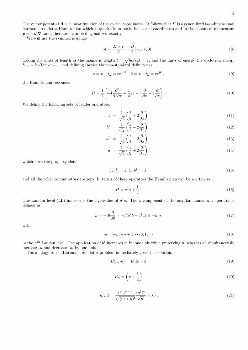

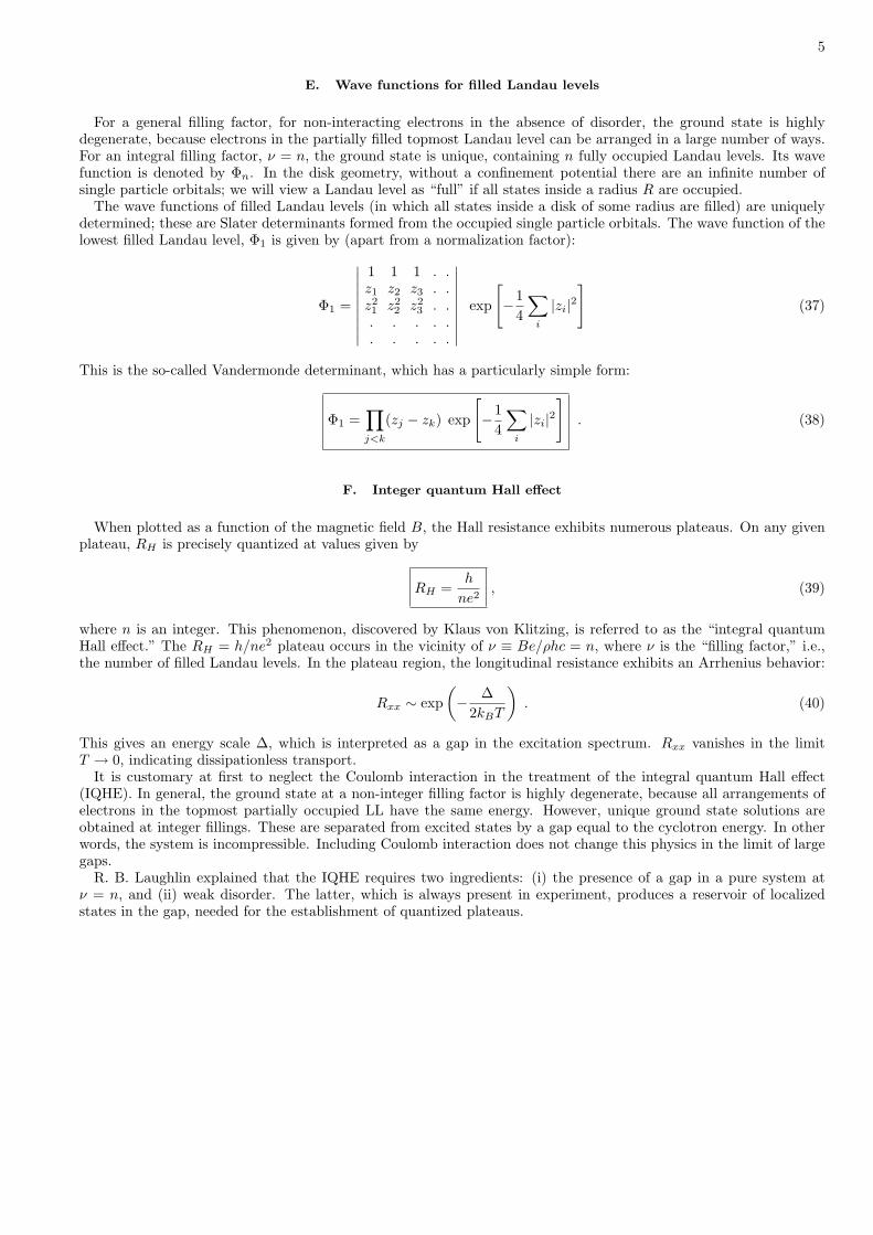


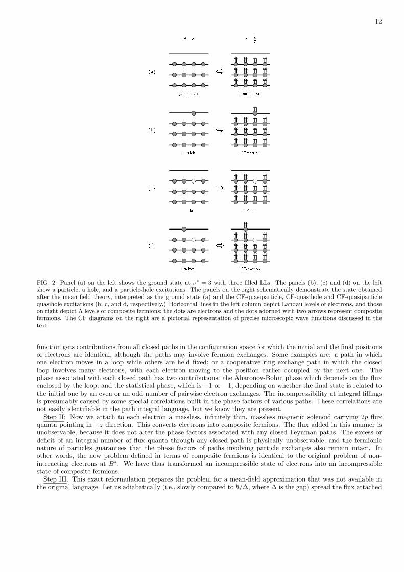


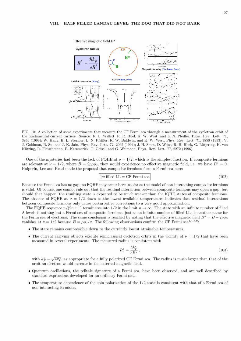


![Fractional Cascading Fractional Cascading I: A Data Structuring Technique Fractional Cascading II: Applications [Chazaelle & Guibas 1986] Dynamic Fractional.](https://static.documents.pub/doc/80x56/56649ea25503460f94ba64dd/fractional-cascading-fractional-cascading-i-a-data-structuring-technique-fractional.jpg)


