3.1 Measures of Central Tendency: Mode, Median, and Mean 3...

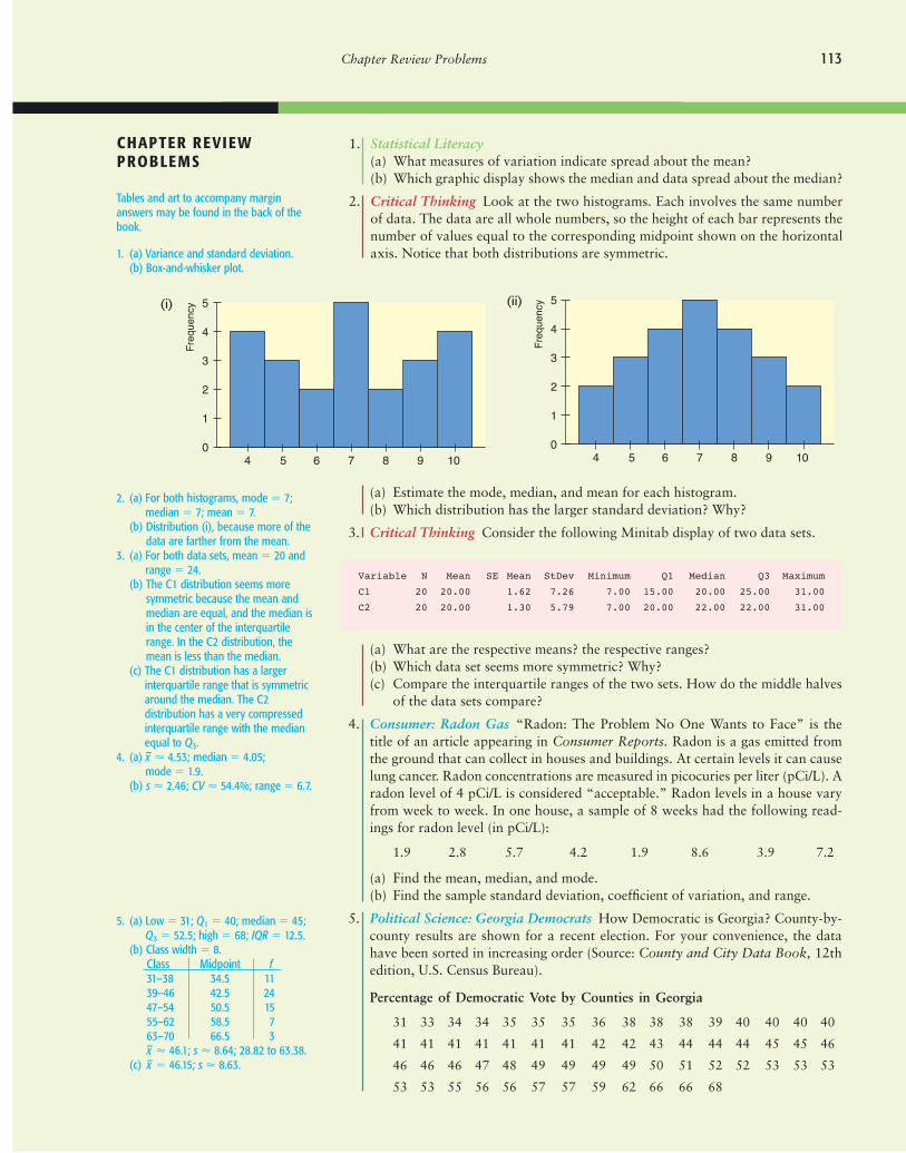
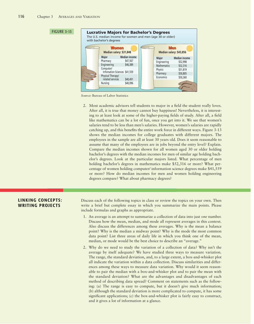
Sherlock Holmes spoke these words to hiscolleague Dr. Watson as the two wereunraveling a mystery. The detective wasimplying that if a single member is drawnat random from a population, we cannotpredict exactly what that member will look

like. However, there are some “average” features ofthe entire population that an individual is likely topossess. The degree of certainty with which we wouldexpect to observe such average features in any indi-vidual depends on our knowledge of the variationamong individuals in the population. SherlockHolmes has led us to two of the most important sta-tistical concepts: average and variation.

While the individual man is an insolvable

puzzle, in the aggregate he becomes a

mathematical certainty. You can, for

example, never foretell what any one man

will do, but you can say with precision

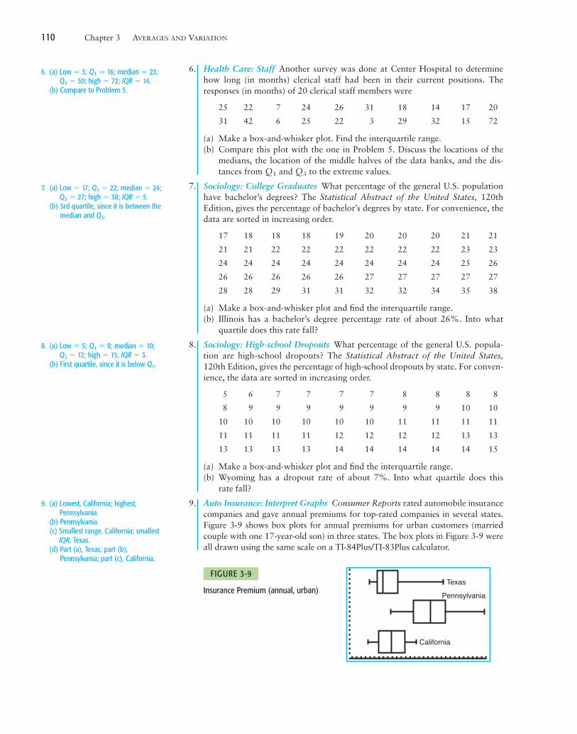
what an average number will be up to.

—Arthur Conan Doyle,The Sign of Four

33.1 Measures of Central Tendency: Mode, Median,

and Mean

3.2 Measures of Variation

3.3 Percentiles and Box-and-Whisker Plots

74

For on-line student resources, visit math.college.hmco.com/students and follow theStatistics links to the Brase/Brase, Understandable Statistics,9th edition web site.

1020437_Ch03_p074-121 7/13/07 4:55 AM Page 74

F O C U S P R O B L E M

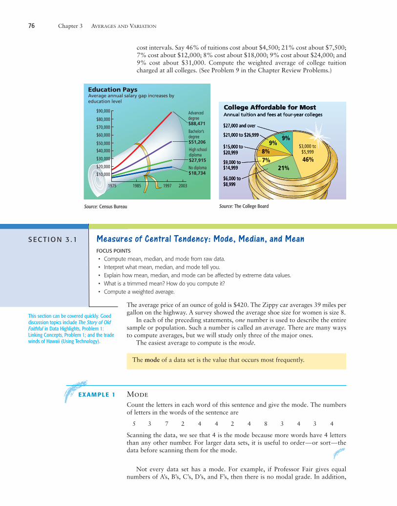
The Educational AdvantageIs it really worth all the effort to get a college degree? From a philosophicalpoint of view, the love of learning is sufficient reason to get a college degree.However, the U.S. Census Bureau also makes another relevant point.Annually, college graduates (bachelor’s degree) earn onaverage $23,291 more than high school graduates. Thismeans college graduates earn about 83.4% more thanhigh school graduates, and according to “EducationPays” on the next page, the gap in earnings is increas-ing. Furthermore, as the College Board indicates, formost Americans college remains relatively affordable.

After completing this chapter, you will be able toanswer the following questions.

(a) Does a college degree guarantee someone an 83.4%increase in earnings over a high school degree?Remember, we are using only averages from censusdata.

(b) Using census data (not shown in “EducationPays”), it is estimated that the standard deviationof college-graduate earnings is about $8,500.Compute a 75% Chebyshev confidence intervalcentered on the mean ($51,206) for bachelor’sdegree earnings.

(c) How much does college tuition cost? That depends,of course, on where you go to college. Construct aweighted average. Using the data from “CollegeAffordable for Most,” estimate midpoints for the

P R E V I E W Q U EST I O N S

What are commonly used measures of central tendency? What do they tell you? (SECTION 3.1)

How do variance and standard deviation measure data spread? Why is this important? (SECTION 3.2)

How do you make a box-and-whisker plot, and what does it tell about the spread of the data? (SECTION 3.3)

75

Averages and Variation

1020437_Ch03_p074-121 7/13/07 4:55 AM Page 75

Education PaysAverage annual salary gap increases byeducation level

Bachelor’sdegree$51,206

High schooldiploma$27,915

No diploma$18,734

$60,000

$70,000

$50,000

$90,000

$80,000

$40,000

$30,000

$20,000

$10,000

1975 1985 1997 2003

Advanceddegree$88,471

$3,000 to$5,999

9%9%

8%7%

21%46%

Source: Census Bureau Source: The College Board

cost intervals. Say 46% of tuitions cost about $4,500; 21% cost about $7,500;7% cost about $12,000; 8% cost about $18,000; 9% cost about $24,000; and9% cost about $31,000. Compute the weighted average of college tuitioncharged at all colleges. (See Problem 9 in the Chapter Review Problems.)

76 Chapter 3 AVERAGES AND VARIATION

S EC T I O N 3 . 1 Measures of Central Tendency: Mode, Median, and MeanFOCUS POINTS

• Compute mean, median, and mode from raw data.• Interpret what mean, median, and mode tell you.• Explain how mean, median, and mode can be affected by extreme data values.• What is a trimmed mean? How do you compute it?• Compute a weighted average.

The average price of an ounce of gold is $420. The Zippy car averages 39 miles pergallon on the highway. A survey showed the average shoe size for women is size 8.

In each of the preceding statements, one number is used to describe the entiresample or population. Such a number is called an average. There are many waysto compute averages, but we will study only three of the major ones.

The easiest average to compute is the mode.

The mode of a data set is the value that occurs most frequently.

EXAMPLE 1 ModeCount the letters in each word of this sentence and give the mode. The numbersof letters in the words of the sentence are

5 3 7 2 4 4 2 4 8 3 4 3 4

Scanning the data, we see that 4 is the mode because more words have 4 lettersthan any other number. For larger data sets, it is useful to order—or sort—thedata before scanning them for the mode.

Not every data set has a mode. For example, if Professor Fair gives equalnumbers of A’s, B’s, C’s, D’s, and F’s, then there is no modal grade. In addition,

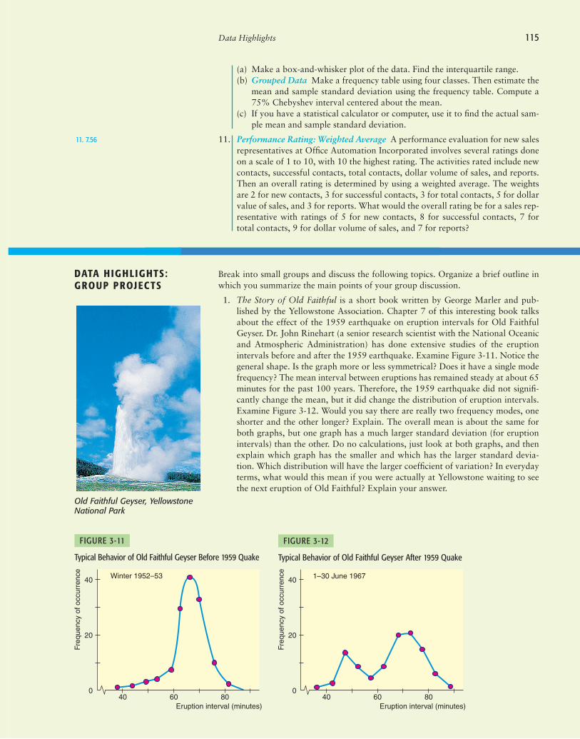
This section can be covered quickly. Gooddiscussion topics include The Story of OldFaithful in Data Highlights, Problem 1:Linking Concepts, Problem 1; and the tradewinds of Hawaii (Using Technology).

1020437_Ch03_p074-121 7/13/07 4:55 AM Page 76

the mode is not very stable. Changing just one number in a data set can changethe mode dramatically. However, the mode is a useful average when we want toknow the most frequently occurring data value, such as the most frequentlyrequested shoe size.

Another average that is useful is the median, or central value, of an ordereddistribution. When you are given the median, you know there are an equal num-ber of data values in the ordered distribution that are above it and below it.

Section 3.1 Measures of Central Tendency: Mode, Median, and Mean 77

Median

PROCEDURE HOW TO FIND THE MEDIAN

The median is the central value of an ordered distribution. To find it,

1. Order the data from smallest to largest.

2. For an odd number of data values in the distribution,

Median ! Middle data value

3. For an even number of data values in the distribution,

Median !Sum of middle two values

2

EXAMPLE 2 MedianWhat do barbecue-flavored potato chips cost? According to Consumer Reports,Volume 66, No. 5, the prices per ounce in cents of the rated chips are

19 19 27 28 18 35

(a) To find the median, we first order the data, and then note that there are an evennumber of entries. So the median is constructed using the two middle values.

18 19 19 27 28 35

middle values

(b) According to Consumer Reports, the brand with the lowest overall taste rat-ing costs 35 cents per ounce. Eliminate that brand, and find the medianprice per ounce for the remaining barbecue-flavored chips. Again order thedata. Note that there are an odd number of entries, so the median is simplythe middle value.

18 19 19 27 28↑⎟

middle value

Median ! middle value ! 19 cents

(c) One ounce of potato chips is considered a small serving. Is it reasonable tobudget about $10.45 to serve the barbecue-flavored chips to 55 people?

Yes, since the median price of the chips is 19 cents per small serving. Thisbudget for chips assumes that there is plenty of other food!

Median !19 " 27

2! 23 cents

The notation x– (read “x tilde”) is sometimesused to designate the median of a data set.

1020437_Ch03_p074-121 7/13/07 4:55 AM Page 77

The median uses the position rather than the specific value of each data entry.If the extreme values of a data set change, the median usually does not change.This is why the median is often used as the average for house prices. If one man-sion costing several million dollars sells in a community of much-lower-pricedhomes, the median selling price for houses in the community would be affectedvery little, if at all.


G U I D E D E X E R C I S E 1 Median and mode

(a) Organize the data from smallest to largestnumber of credit hours.

(b) Since there are an (odd, even) numberof values, we add the two middle values anddivide by 2 to get the median. What is themedian credit hour load?

(c) What is the mode of this distribution? Is itdifferent from the median? If the budgetcommittee is going to fund the school accordingto the average student credit hour load (moremoney for higher loads), which of these twoaverages do you think the college will use?

12 12 12 12 12 12 12 12 12 12

13 13 13 13 14 14 14 14 15 15

15 15 15 15 16 16 16 16 17 17

17 17 17 18 18 18 19 19 20 20

There are an even number of entries. The twomiddle values are circled in part (a).

The mode is 12. It is different from the median.Since the median is higher, the school will probablyuse it and indicate that the average being used is themedian.

Median !15 " 15

2! 15

Belleview College must make a report to the budget committee about the average credit hour loada full-time student carries. (A 12-credit-hour load is the minimum requirement for full-time status.For the same tuition, students may take up to 20 credit hours.) A random sample of 40 studentsyielded the following information (in credit hours):

17 12 14 17 13 16 18 20 13 12

12 17 16 15 14 12 12 13 17 14

15 12 15 16 12 18 20 19 12 15

18 14 16 17 15 19 12 13 12 15

Note: For small ordered data sets, we can easily scan the set to find the loca-tion of the median. However, for large ordered data sets of size n, it is convenientto have a formula to find the middle of the data set.

For an ordered data set of size n,

For instance, if then the middle value is the or 50th data valuein the ordered data. If then tells us that the twomiddle values are in the 50th and 51st positions.

(100 " 1)/2 ! 50.5n ! 100,(99 " 1)/2n ! 99,

Position of the middle value !n " 1

2

1020437_Ch03_p074-121 7/13/07 4:55 AM Page 78

An average that uses the exact value of each entry is the mean (sometimescalled the arithmetic mean). To compute the mean, we add the values of all theentries and then divide by the number of entries.

The mean is the average usually used to compute a test average.

Mean !Sum of all entriesNumber of entries


Mean

Most students will recognize thecomputation procedure for the mean as theprocess they follow to compute a simpleaverage of test grades.

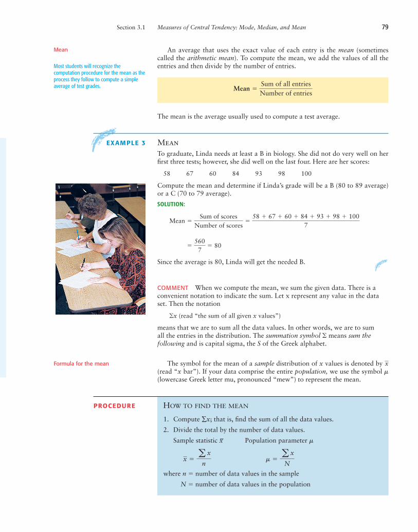
EXAMPLE 3 MeanTo graduate, Linda needs at least a B in biology. She did not do very well on herfirst three tests; however, she did well on the last four. Here are her scores:

58 67 60 84 93 98 100

Compute the mean and determine if Linda’s grade will be a B (80 to 89 average)or a C (70 to 79 average).

SOLUTION:

Since the average is 80, Linda will get the needed B.

COMMENT When we compute the mean, we sum the given data. There is aconvenient notation to indicate the sum. Let x represent any value in the dataset. Then the notation

!x (read “the sum of all given x values”)

means that we are to sum all the data values. In other words, we are to sumall the entries in the distribution. The summation symbol ! means sum thefollowing and is capital sigma, the S of the Greek alphabet.

The symbol for the mean of a sample distribution of x values is denoted by(read “x bar”). If your data comprise the entire population, we use the symbol m(lowercase Greek letter mu, pronounced “mew”) to represent the mean.

x

!5607

! 80

Mean !Sum of scores

Number of scores!

58 " 67 " 60 " 84 " 93 " 98 " 1007

PROCEDURE HOW TO FIND THE MEAN

1. Compute ∑x; that is, find the sum of all the data values.

2. Divide the total by the number of data values.

Sample statistic x– Population parameter m

where n ! number of data values in the sample

N ! number of data values in the population

m !a x

Nx !

a x

n

Formula for the mean

1020437_Ch03_p074-121 7/13/07 4:55 AM Page 79

CALCULATOR NOTE It is very easy to compute the mean on any calculator:Simply add the data values and divide the total by the number of data.However, on calculators with a statistics mode, you place the calculator inthat mode, enter the data, and then press the key for the mean. The key isusually designated . Because the formula for the population mean is the sameas that for the sample mean, the same key gives the value for m.

We have seen three averages: the mode, the median, and the mean. For laterwork, the mean is the most important. A disadvantage of the mean, however, isthat it can be affected by exceptional values.

A resistant measure is one that is not influenced by extremely high or low datavalues. The mean is not a resistant measure of center because we can make themean as large as we want by changing the size of only one data value. Themedian, on the other hand, is more resistant. However, a disadvantage ofthe median is that it is not sensitive to the specific size of a data value.

A measure of center that is more resistant than the mean but still sensitive tospecific data values is the trimmed mean. A trimmed mean is the mean of the datavalues left after “trimming” a specified percentage of the smallest and largest datavalues from the data set. Usually a 5% trimmed mean is used. This implies thatwe trim the lowest 5% of the data as well as the highest 5% of the data. A simi-lar procedure is used for a 10% trimmed mean.

x


Resistant measure

This is a good time to review calculatorprocedures with students, with particularemphasis on order of operations.

Trimmed mean

PROCEDURE HOW TO COMPUTE A 5% TRIMMED MEAN


2. Delete the bottom 5% of the data and the top 5% of the data. Note: Ifthe calculation of 5% of the number of data values does not produce awhole number, round to the nearest integer.

3. Compute the mean of the remaining 90% of the data.

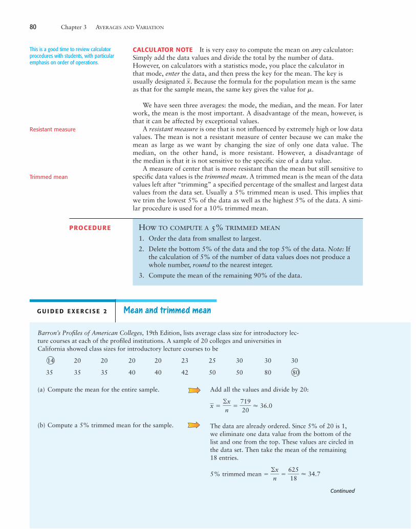
G U I D E D E X E R C I S E 2 Mean and trimmed mean

(a) Compute the mean for the entire sample.

(b) Compute a 5% trimmed mean for the sample.

Add all the values and divide by 20:

The data are already ordered. Since 5% of 20 is 1,we eliminate one data value from the bottom of thelist and one from the top. These values are circled inthe data set. Then take the mean of the remaining18 entries.

5% trimmed mean !!xn

!62518

" 34.7

x !!xn

!71920

" 36.0

Barron’s Profiles of American Colleges, 19th Edition, lists average class size for introductory lec-ture courses at each of the profiled institutions. A sample of 20 colleges and universities inCalifornia showed class sizes for introductory lecture courses to be

14 20 20 20 20 23 25 30 30 30

35 35 35 40 40 42 50 50 80 80

Continued

1020437_Ch03_p074-121 7/13/07 4:55 AM Page 80

TECH NOTES Minitab, Excel, and TI-84Plus/TI-83Plus calculators all provide the mean and medianof a data set. Minitab and Excel also provide the mode. The TI-84Plus/TI-83Pluscalculators sort data, so you can easily scan the sorted data for the mode. Minitabprovides the 5% trimmed mean, as does Excel.

All this technology is a wonderful aid for analyzing data. However, a measure-ment has no meaning if you do not know what it represents or how a change in datavalues might affect the measurement. The defining formulas and procedures forcomputing the measures tell you a great deal about the measures. Even if you use acalculator to evaluate all the statistical measures, pay attention to the informationthe formulas and procedures give you about the components or features of themeasurement.


(c) Find the median for the original data set.

(d) Find the median of the 5% trimmed data set.Does the median change when you trim thedata?

(e) Is the trimmed mean or the original mean closerto the median?

Note that the data are already ordered.

The median is still 32.5. Notice that trimming thesame number of entries from both ends leaves themiddle position of the data set unchanged.

The trimmed mean is closer to the median.

Median !30 " 35

2! 32.5

G U I D E D E X E R C I S E 2 continued

CRITICALTHINKING In Chapter 1, we examined four levels of data: nominal, ordinal, interval, and

ratio. The mode (if it exists) can be used with all four levels, including nominal.For instance, the modal color of all passenger cars sold last year might be blue.The median may be used with data at the ordinal level or above. If we ranked thepassenger cars in order of customer satisfaction level, we could identify themedian satisfaction level. For the mean, our data need to be at the interval orratio level (although there are exceptions in which the mean of ordinal-level datais computed). We can certainly find the mean model year of used passenger carssold or the mean price of new passenger cars.

Another issue of concern is that of taking the average of averages. For instance,if the values $520, $640, $730, $890, and $920 represent the mean monthly rentsfor five different apartment complexes, we can’t say that $740 (the mean of thefive numbers) is the mean monthly rent of all the apartments. We need to know thenumber of apartments in each complex before we can determine an average basedon the number of apartments renting at each designated amount.

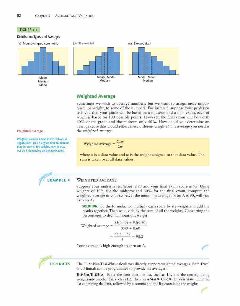
In general, when a data distribution is mound-shaped symmetrical, the val-ues for the mean, median, and mode are the same or almost the same. Forskewed-left distributions, the mean is less than the median and the median is lessthan the mode. For skewed-right distributions, the mode is the smallest value,the median is the next largest, and the mean is the largest. Figure 3-1 shows thegeneral relationships among the mean, median, and mode for different types ofdistributions.

Data types and averages

Distribution shapes and averages

The ideas at the right can be used to reviewlevels of measurement and link some ofthose concepts to the material in thissection.

1020437_Ch03_p074-121 7/13/07 4:55 AM Page 81

Weighted AverageSometimes we wish to average numbers, but we want to assign more impor-tance, or weight, to some of the numbers. For instance, suppose your professortells you that your grade will be based on a midterm and a final exam, each ofwhich is based on 100 possible points. However, the final exam will be worth60% of the grade and the midterm only 40%. How could you determine anaverage score that would reflect these different weights? The average you need isthe weighted average.

where x is a data value and w is the weight assigned to that data value. Thesum is taken over all data values.

Weighted average !!xw!w


Weighted average

(a) Mound-shaped symmetric

MeanMedianMode

(b) Skewed left

ModeMeanMedian

(c) Skewed right

Mode MeanMedian

Distribution Types and Averages

FIGURE 3-1

EXAMPLE 4 Weighted averageSuppose your midterm test score is 83 and your final exam score is 95. Usingweights of 40% for the midterm and 60% for the final exam, compute theweighted average of your scores. If the minimum average for an A is 90, will youearn an A?

SOLUTION: By the formula, we multiply each score by its weight and add theresults together. Then we divide by the sum of all the weights. Converting thepercentages to decimal notation, we get

Your average is high enough to earn an A.

!33.2 " 57

1! 90.2

Weighted average !8310.402 " 9510.602

0.40 " 0.60

Weighted averages have many real-worldapplications. This is a good time to mentionthat the sum of the weights may or maynot be 1, depending on the application.

TECH NOTES The TI-84Plus/TI-83Plus calculators directly support weighted averages. Both Exceland Minitab can be programmed to provide the averages.

TI-84Plus/TI-83Plus Enter the data into one list, such as L1, and the correspondingweights into another list, such as L2. Then press Stat ➤ Calc ➤ 1: 1-Var Stats. Enter thelist containing the data, followed by a comma and the list containing the weights.

1020437_Ch03_p074-121 7/13/07 4:55 AM Page 82


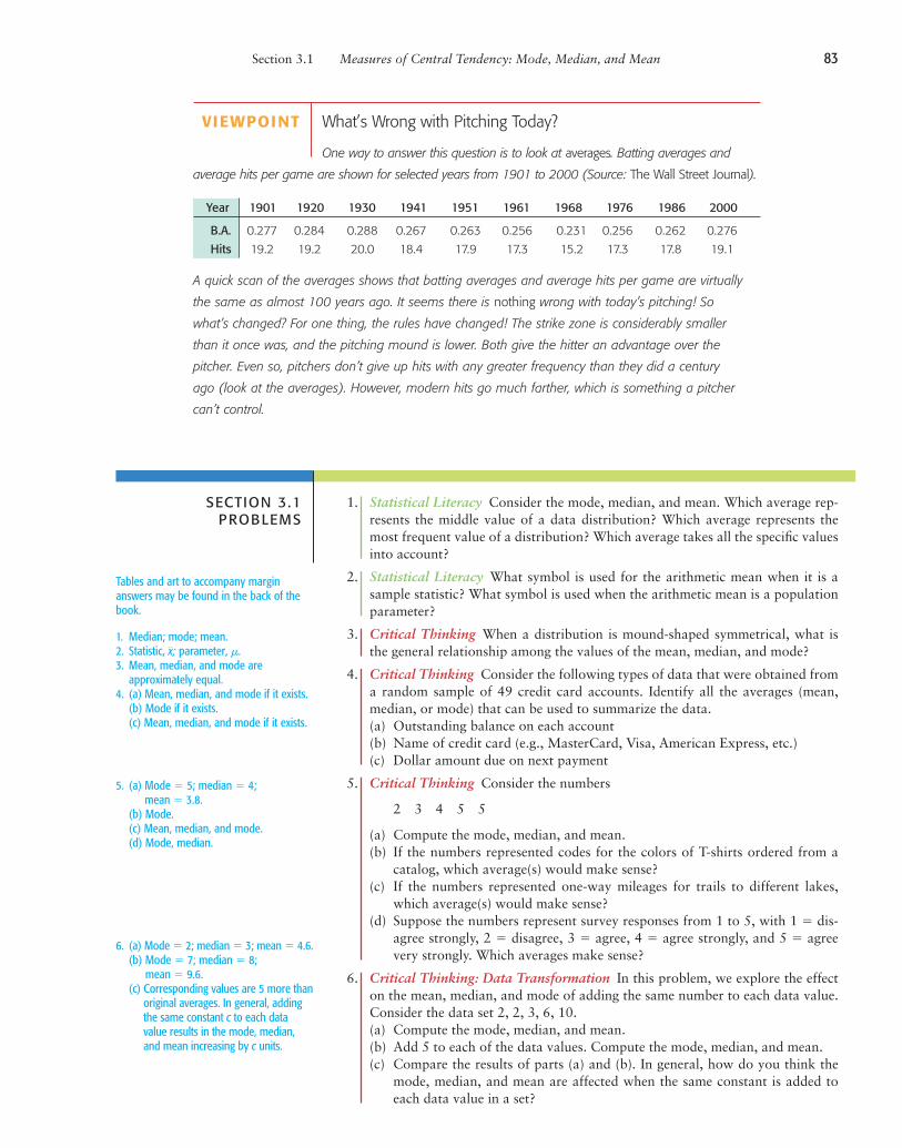
VIEWPOINT What’s Wrong with Pitching Today?

One way to answer this question is to look at averages. Batting averages and

average hits per game are shown for selected years from 1901 to 2000 (Source: The Wall Street Journal).

Year 1901 1920 1930 1941 1951 1961 1968 1976 1986 2000

B.A. 0.277 0.284 0.288 0.267 0.263 0.256 0.231 0.256 0.262 0.276Hits 19.2 19.2 20.0 18.4 17.9 17.3 15.2 17.3 17.8 19.1

A quick scan of the averages shows that batting averages and average hits per game are virtually

the same as almost 100 years ago. It seems there is nothing wrong with today’s pitching! So

what’s changed? For one thing, the rules have changed! The strike zone is considerably smaller

than it once was, and the pitching mound is lower. Both give the hitter an advantage over the

pitcher. Even so, pitchers don’t give up hits with any greater frequency than they did a century

ago (look at the averages). However, modern hits go much farther, which is something a pitcher

can’t control.

SECTION 3.1 PROBLEMS

1. Statistical Literacy Consider the mode, median, and mean. Which average rep-resents the middle value of a data distribution? Which average represents themost frequent value of a distribution? Which average takes all the specific valuesinto account?

2. Statistical Literacy What symbol is used for the arithmetic mean when it is asample statistic? What symbol is used when the arithmetic mean is a populationparameter?

3. Critical Thinking When a distribution is mound-shaped symmetrical, what isthe general relationship among the values of the mean, median, and mode?

4. Critical Thinking Consider the following types of data that were obtained froma random sample of 49 credit card accounts. Identify all the averages (mean,median, or mode) that can be used to summarize the data.(a) Outstanding balance on each account(b) Name of credit card (e.g., MasterCard, Visa, American Express, etc.)(c) Dollar amount due on next payment

5. Critical Thinking Consider the numbers

2 3 4 5 5

(a) Compute the mode, median, and mean.(b) If the numbers represented codes for the colors of T-shirts ordered from a

catalog, which average(s) would make sense?(c) If the numbers represented one-way mileages for trails to different lakes,

which average(s) would make sense?(d) Suppose the numbers represent survey responses from 1 to 5, with 1 ! dis-

agree strongly, 2 ! disagree, 3 ! agree, 4 ! agree strongly, and 5 ! agreevery strongly. Which averages make sense?

6. Critical Thinking: Data Transformation In this problem, we explore the effecton the mean, median, and mode of adding the same number to each data value.Consider the data set 2, 2, 3, 6, 10.(a) Compute the mode, median, and mean.(b) Add 5 to each of the data values. Compute the mode, median, and mean.(c) Compare the results of parts (a) and (b). In general, how do you think the

mode, median, and mean are affected when the same constant is added toeach data value in a set?

Tables and art to accompany marginanswers may be found in the back of thebook.

1. Median; mode; mean.2. Statistic, ; parameter, m.3. Mean, median, and mode are

approximately equal.4. (a) Mean, median, and mode if it exists.

(b) Mode if it exists.(c) Mean, median, and mode if it exists.

x

5. (a) Mode ! 5; median ! 4; mean ! 3.8.

(b) Mode.(c) Mean, median, and mode.(d) Mode, median.

6. (a) Mode ! 2; median ! 3; mean ! 4.6.(b) Mode ! 7; median ! 8;

mean ! 9.6.(c) Corresponding values are 5 more than

original averages. In general, addingthe same constant c to each datavalue results in the mode, median,and mean increasing by c units.

1020437_Ch03_p074-121 7/13/07 4:55 AM Page 83

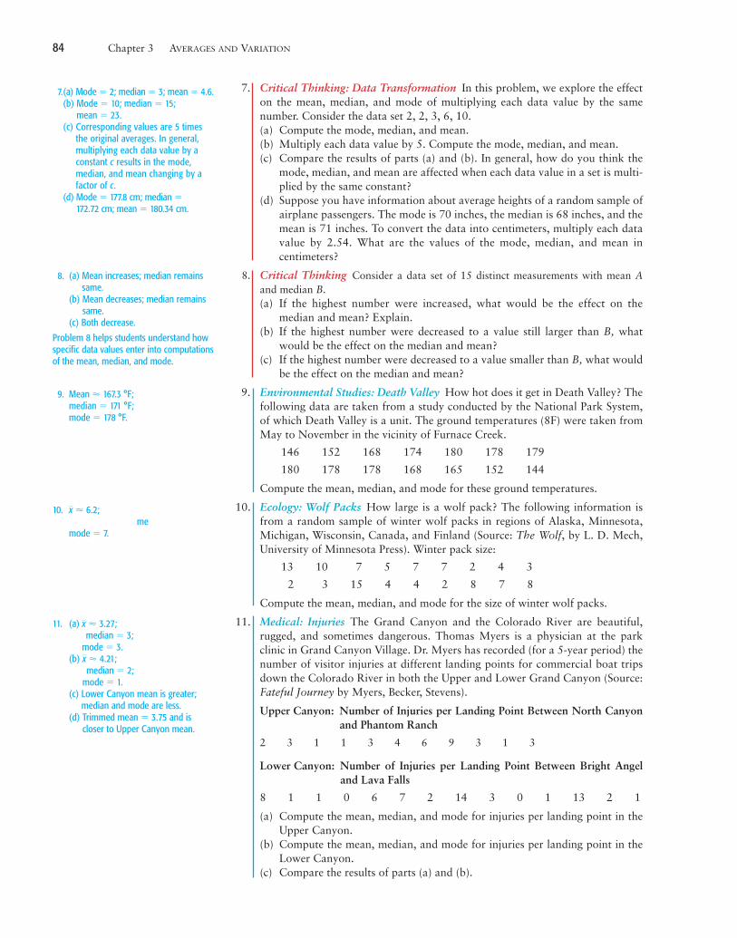
7. Critical Thinking: Data Transformation In this problem, we explore the effecton the mean, median, and mode of multiplying each data value by the samenumber. Consider the data set 2, 2, 3, 6, 10.(a) Compute the mode, median, and mean.(b) Multiply each data value by 5. Compute the mode, median, and mean.(c) Compare the results of parts (a) and (b). In general, how do you think the

mode, median, and mean are affected when each data value in a set is multi-plied by the same constant?

(d) Suppose you have information about average heights of a random sample ofairplane passengers. The mode is 70 inches, the median is 68 inches, and themean is 71 inches. To convert the data into centimeters, multiply each datavalue by 2.54. What are the values of the mode, median, and mean incentimeters?

8. Critical Thinking Consider a data set of 15 distinct measurements with mean Aand median B.(a) If the highest number were increased, what would be the effect on the

median and mean? Explain.(b) If the highest number were decreased to a value still larger than B, what

would be the effect on the median and mean?(c) If the highest number were decreased to a value smaller than B, what would

be the effect on the median and mean?

9. Environmental Studies: Death Valley How hot does it get in Death Valley? Thefollowing data are taken from a study conducted by the National Park System,of which Death Valley is a unit. The ground temperatures (8F) were taken fromMay to November in the vicinity of Furnace Creek.

146 152 168 174 180 178 179

180 178 178 168 165 152 144

Compute the mean, median, and mode for these ground temperatures.

10. Ecology: Wolf Packs How large is a wolf pack? The following information isfrom a random sample of winter wolf packs in regions of Alaska, Minnesota,Michigan, Wisconsin, Canada, and Finland (Source: The Wolf, by L. D. Mech,University of Minnesota Press). Winter pack size:

13 10 7 5 7 7 2 4 3

2 3 15 4 4 2 8 7 8

Compute the mean, median, and mode for the size of winter wolf packs.

11. Medical: Injuries The Grand Canyon and the Colorado River are beautiful,rugged, and sometimes dangerous. Thomas Myers is a physician at the parkclinic in Grand Canyon Village. Dr. Myers has recorded (for a 5-year period) thenumber of visitor injuries at different landing points for commercial boat tripsdown the Colorado River in both the Upper and Lower Grand Canyon (Source:Fateful Journey by Myers, Becker, Stevens).

Upper Canyon: Number of Injuries per Landing Point Between North Canyonand Phantom Ranch

2 3 1 1 3 4 6 9 3 1 3

Lower Canyon: Number of Injuries per Landing Point Between Bright Angeland Lava Falls

8 1 1 0 6 7 2 14 3 0 1 13 2 1

(a) Compute the mean, median, and mode for injuries per landing point in theUpper Canyon.

(b) Compute the mean, median, and mode for injuries per landing point in theLower Canyon.

(c) Compare the results of parts (a) and (b).


7.(a) Mode ! 2; median ! 3; mean ! 4.6.(b) Mode ! 10; median ! 15;

mean ! 23.(c) Corresponding values are 5 times

the original averages. In general,multiplying each data value by aconstant c results in the mode,median, and mean changing by afactor of c.

(d) Mode ! 177.8 cm; median !172.72 cm; mean ! 180.34 cm.

8. (a) Mean increases; median remainssame.

(b) Mean decreases; median remainssame.

(c) Both decrease.Problem 8 helps students understand howspecific data values enter into computationsof the mean, median, and mode.

9. Mean " 167.3 °F;median ! 171 °F;mode ! 178 °F.

10. " 6.2;me

mode ! 7.

x

11. (a) " 3.27;median ! 3;

mode ! 3.(b) " 4.21;

median ! 2;mode ! 1.

(c) Lower Canyon mean is greater;median and mode are less.

(d) Trimmed mean ! 3.75 and iscloser to Upper Canyon mean.

x

x

1020437_Ch03_p074-121 7/13/07 4:55 AM Page 84

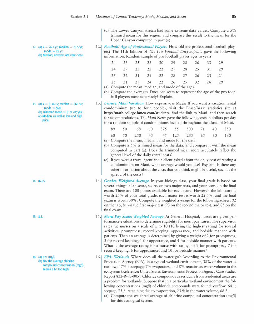
(d) The Lower Canyon stretch had some extreme data values. Compute a 5%trimmed mean for this region, and compare this result to the mean for theUpper Canyon computed in part (a).

12. Football: Age of Professional Players How old are professional football play-ers? The 11th Edition of The Pro Football Encyclopedia gave the followinginformation. Random sample of pro football player ages in years:

24 23 25 23 30 29 28 26 33 29

24 37 25 23 22 27 28 25 31 29

25 22 31 29 22 28 27 26 23 21

25 21 25 24 22 26 25 32 26 29(a) Compute the mean, median, and mode of the ages.(b) Compare the averages. Does one seem to represent the age of the pro foot-

ball players most accurately? Explain.

13. Leisure: Maui Vacation How expensive is Maui? If you want a vacation rentalcondominium (up to four people), visit the Brase/Brase statistics site athttp://math.college.hmco.com/students, find the link to Maui, and then searchfor accommodations. The Maui News gave the following costs in dollars per dayfor a random sample of condominiums located throughout the island of Maui.

89 50 68 60 375 55 500 71 40 350

60 50 250 45 45 125 235 65 60 130(a) Compute the mean, median, and mode for the data.(b) Compute a 5% trimmed mean for the data, and compare it with the mean

computed in part (a). Does the trimmed mean more accurately reflect thegeneral level of the daily rental costs?

(c) If you were a travel agent and a client asked about the daily cost of renting acondominium on Maui, what average would you use? Explain. Is there anyother information about the costs that you think might be useful, such as thespread of the costs?

14. Grades: Weighted Average In your biology class, your final grade is based onseveral things: a lab score, scores on two major tests, and your score on the finalexam. There are 100 points available for each score. However, the lab score isworth 25% of your total grade, each major test is worth 22.5%, and the finalexam is worth 30%. Compute the weighted average for the following scores: 92on the lab, 81 on the first major test, 93 on the second major test, and 85 on thefinal exam.

15. Merit Pay Scale: Weighted Average At General Hospital, nurses are given per-formance evaluations to determine eligibility for merit pay raises. The supervisorrates the nurses on a scale of 1 to 10 (10 being the highest rating) for severalactivities: promptness, record keeping, appearance, and bedside manner withpatients. Then an average is determined by giving a weight of 2 for promptness,3 for record keeping, 1 for appearance, and 4 for bedside manner with patients.What is the average rating for a nurse with ratings of 9 for promptness, 7 forrecord keeping, 6 for appearance, and 10 for bedside manner?

16. EPA: Wetlands Where does all the water go? According to the EnvironmentalProtection Agency (EPA), in a typical wetland environment, 38% of the water isoutflow; 47% is seepage; 7% evaporates; and 8% remains as water volume in theecosystem (Reference: United States Environmental Protection Agency Case StudiesReport 832-R-93-005). Chloride compounds as residuals from residential areas area problem for wetlands. Suppose that in a particular wetland environment the fol-lowing concentrations (mg/l) of chloride compounds were found: outflow, 64.1;seepage, 75.8; remaining due to evaporation, 23.9; in the water volume, 68.2.(a) Compute the weighted average of chlorine compound concentration (mg/l)

for this ecological system.


12. (a) " 26.3 yr; median ! 25.5 yr;mode ! 25 yr.

(b) Median; answers are very close.

x

13. (a) ! $136.15; median ! $66.50;mode ! $60.

(b) Trimmed mean " $121.28; yes.(c) Median, as well as low and high

price.

x

14. 87.65.

15. 8.5.

16. (a) 67.1 mg/l.(b) No; the average chlorine

compound concentration (mg/l)seems a bit too high.

1020437_Ch03_p074-121 7/13/07 4:55 AM Page 85

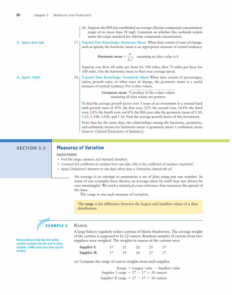
(b) Suppose the EPA has established an average chlorine compound concentrationtarget of no more than 58 mg/l. Comment on whether this wetlands systemmeets the target standard for chlorine compound concentration.

17. Expand Your Knowledge: Harmonic Mean When data consist of rates of change,such as speeds, the harmonic mean is an appropriate measure of central tendency.

Harmonic mean assuming no data value is 0

Suppose you drive 60 miles per hour for 100 miles, then 75 miles per hour for100 miles. Use the harmonic mean to find your average speed.

18. Expand Your Knowledge: Geometric Mean When data consist of percentages,ratios, growth rates, or other rates of change, the geometric mean is a usefulmeasure of central tendency. For n data values,

Geometric mean assuming all data values are positive

To find the average growth factor over 5 years of an investment in a mutual fundwith growth rates of 10% the first year, 12% the second year, 14.8% the thirdyear, 3.8% the fourth year, and 6% the fifth year, take the geometric mean of 1.10,1.12, 1.148, 1.038, and 1.16. Find the average growth factor of this investment.

Note that for the same data, the relationships among the harmonic, geometric,and arithmetic means are: harmonic mean # geometric mean # arithmetic mean(Source: Oxford Dictionary of Statistics).

2n product of the n data values

!n

! 1x,


17. Approx. 66.67 mph.

18. Approx. 1.09247.

S EC T I O N 3 . 2 Measures of VariationFOCUS POINTS

• Find the range, variance, and standard deviation.• Compute the coefficient of variation from raw data. Why is the coefficient of variation important?• Apply Chebyshev’s theorem to raw data. What does a Chebyshev interval tell us?

An average is an attempt to summarize a set of data using just one number. Assome of our examples have shown, an average taken by itself may not always bevery meaningful. We need a statistical cross-reference that measures the spread ofthe data.

The range is one such measure of variation.

The range is the difference between the largest and smallest values of a datadistribution.

EXAMPLE 5 RangeA large bakery regularly orders cartons of Maine blueberries. The average weightof the cartons is supposed to be 22 ounces. Random samples of cartons from twosuppliers were weighed. The weights in ounces of the cartons were

Supplier I: 17 22 22 22 27

Supplier II: 17 19 20 27 27

(a) Compute the range of carton weights from each supplier.

Range ! Largest value $ Smallest valueSupplier I range ! 27 $ 17 ! 10 ounces

Supplier II range ! 27 $ 17 ! 10 ounces

Most professors find that this sectioncontains concepts that are new to manystudents. A little more class time may beneeded.

1020437_Ch03_p074-121 7/13/07 4:55 AM Page 86

(b) Compute the mean weight of cartons from each supplier. In both cases themean is 22 ounces.

(c) Look at the two samples again. The samples have the same range and mean.How do they differ? The bakery uses one carton of blueberries in each blue-berry muffin recipe. It is important that the cartons be of consistent weight sothat the muffins turn out right.

Supplier I provides more cartons that have weights closer to the mean. Or, putanother way, the weights of cartons from Supplier I are more clustered aroundthe mean. The bakery might find Supplier I more satisfactory.

As we see in Example 5, although the range tells the difference between thelargest and smallest values in a distribution, it does not tell us how much othervalues vary from one another or from the mean.

Variance and Standard DeviationWe need a measure of the distribution or spread of data around an expectedvalue (either or m). The variance and standard deviation provide suchmeasures. Formulas and rationale for these measures are described in the nextProcedure display. Then, examples and guided exercises show how to computeand interpret these measures.

As we will see later, the formulas for variance and standard deviation differslightly depending on whether we are using a sample or the entire population.

PROCEDURE HOW TO COMPUTE THE SAMPLE VARIANCE AND SAMPLESTANDARD DEVIATION

x

Section 3.2 Measures of Variation 87

Blueberry patch

Quantity Description

x The variable x represents a data value or outcome.Mean This is the average of the data values, or what you ”expect” to

happen the next time you conduct the statistical experiment. Notethat n is the sample size.This is the difference between what happened and what youexpected to happen. This represents a “deviation” away from whatyou “expect” and is a measure of risk.The expression is called the sum of squares. The

quantity is squared to make it nonnegative. The sum isover all the data. If you don’t square , then the sum

because the negative values cancel thepositive values. This occurs even if some values are large,indicating a large deviation or risk.

Sum of squares This is an algebraic simplification of the sum of squares thatis easier to compute.

or The defining formula for the sum of squares is the upper one.The computation formula for the sum of squares is the lowerone. Both formulas give the same result.

Sample variance The sample variance is s2. The variance can be thought of as a kind of average of the values. However, for technical

reasons, we divide the sum by the quantity n $ 1 rather than n.or This gives us the best mathematical estimate for the sample

variance.s2 !

!x2 $ (!x)2%nn $ 1

(x $ x)2s2 !

!(x $ x )2

n $ 1

! x 2 $

(! x)2

n

!(x $ x )2

(x $ x)!(x $ x) is equal to 0

(x $ x)(x $ x)

!(x $ x)2!(x $ x )2

x $ x

x !! xn

Continue

Variance and standard deviation

There are many ways to measure dataspread, and s is only one way (the range isanother way). However, just as standardtime is the time to which most people refer,standard deviation is the measure of dataspread to which most people refer.

1020437_Ch03_p074-121 7/13/07 4:55 AM Page 87

The defining formula for the variance is the upper one. Thecomputation formula for the variance is the lower one. Bothformulas give the same result.

Sample standard This is sample standard deviation, s. Why do we take the squaredeviation root? Well, if the original x units were, say, days or dollars, then the

s2 units would be days squared or dollars squared (wow, what’sthat?). We take the square root to return to the original units of thedata measurements. The standard deviation can be thought of as a

or measure of variability or risk. Larger values of s imply greater variabil-ity in the data.

The defining formula for the standard deviation is the upperone. The computation formula for the standard deviation is the

s ! v!x2 $ (!x)2%nn $ 1

s ! v!( x $ x )2

n $ 1


P R O C E D U R E continued

COMMENT Why is s called a sample standard deviation? First, it is com-puted from sample data. Then why do we use the word standard in thename? We know s is a measure of deviation or risk. You should be awarethat there are other statistical measures of risk that we have not yet men-tioned. However, s is the one that everyone uses, so it is called the “stan-dard” (like standard time).

In statistics, the sample standard deviation and sample variance are used todescribe the spread of data about the mean The next example shows how tofind these quantities by using the defining formulas. Guided Exercise 3 showshow to use the computation formulas.

As you will discover, for “hand” calculations, the computation formulas fors2 and s are much easier to use. However, the defining formulas for s2 and semphasize the fact that the variance and standard deviation are based on the dif-ferences between each data value and the mean.

x.

Some students have trouble comprehendingthe information contained in a formula. Itmay be useful to verbalize the formula for s.It says to compare each data value to themean, square the difference, sum thesquares of the differences, then divide by thequantity (n $ 1) and, finally, take thesquare root of the result.

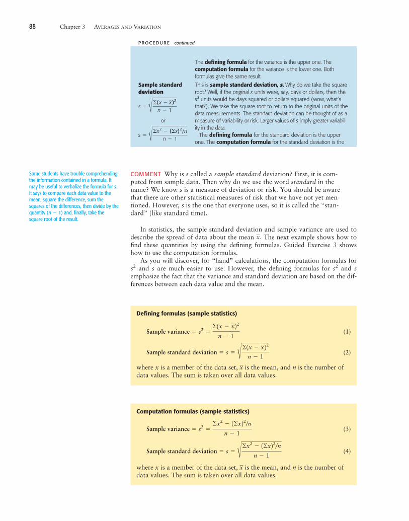
Defining formulas (sample statistics)

(1)

(2)

where x is a member of the data set, is the mean, and n is the number ofdata values. The sum is taken over all data values.

x

Sample standard deviation ! s ! v!1x $ x22n $ 1

Sample variance ! s2 !!1x $ x22

n $ 1

Computation formulas (sample statistics)

(3)

(4)

where x is a member of the data set, is the mean, and n is the number ofdata values. The sum is taken over all data values.

x

Sample standard deviation ! s ! v!x2 $ 1!x22%nn $ 1

Sample variance ! s2 !!x2 $ 1!x22%n

n $ 1

1020437_Ch03_p074-121 7/13/07 4:55 AM Page 88


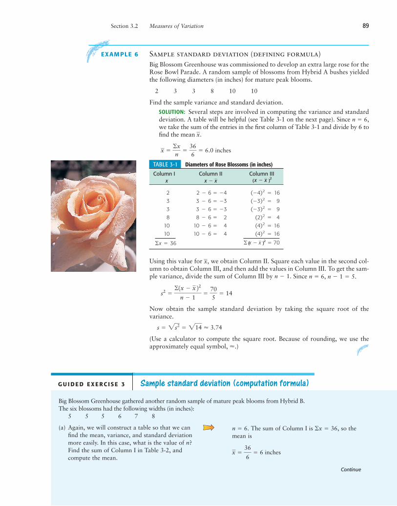
EXAMPLE 6 Sample standard deviation (defining formula)Big Blossom Greenhouse was commissioned to develop an extra large rose for theRose Bowl Parade. A random sample of blossoms from Hybrid A bushes yieldedthe following diameters (in inches) for mature peak blooms.

2 3 3 8 10 10

Find the sample variance and standard deviation.SOLUTION: Several steps are involved in computing the variance and standarddeviation. A table will be helpful (see Table 3-1 on the next page). Since we take the sum of the entries in the first column of Table 3-1 and divide by 6 tofind the mean

x !!xn

!366

! 6.0 inches

x.

n ! 6,

TABLE 3-1 Diameters of Rose Blossoms (in inches)

Column I Column II Column III x

2 2 $ 6 ! $4 ($4)2 ! 163 3 $ 6 ! $3 ($3)2 ! 93 3 $ 6 ! $3 ($3)2 ! 98 8 $ 6 ! 2 (2)2 ! 4

10 10 $ 6 ! 4 (4)2 ! 1610 10 $ 6 ! 4 (4)2 ! 16

!x ! 36 !(x $ x )2 ! 70

(x $ x)2x $ x

Using this value for we obtain Column II. Square each value in the second col-umn to obtain Column III, and then add the values in Column III. To get the sam-ple variance, divide the sum of Column III by Since

Now obtain the sample standard deviation by taking the square root of thevariance.

(Use a calculator to compute the square root. Because of rounding, we use theapproximately equal symbol, ".)

s ! 2s2 ! 214 " 3.74

s2 !!1x $ x 22

n $ 1!

705

! 14

n $ 1 ! 5.n ! 6,n $ 1.

x,

G U I D E D E X E R C I S E 3 Sample standard deviation (computation formula)Big Blossom Greenhouse gathered another random sample of mature peak blooms from Hybrid B.The six blossoms had the following widths (in inches):

5 5 5 6 7 8

(a) Again, we will construct a table so that we canfind the mean, variance, and standard deviationmore easily. In this case, what is the value of n?Find the sum of Column I in Table 3-2, andcompute the mean.

Continue

n ! 6. The sum of Column I is !x ! 36, so themean is

x !36

6! 6 inches

1020437_Ch03_p074-121 7/13/07 4:55 AM Page 89

Let’s summarize and compare the results of Guided Exercise 3 and Example6. The greenhouse found the following blossom diameters for Hybrid A andHybrid B:

Hybrid A: Mean, 6.0 inches; standard deviation, 3.74 inchesHybrid B: Mean, 6.0 inches; standard deviation, 1.26 inches

In both cases, the means are the same: 6 inches. But the first hybrid has a largerstandard deviation. This means that the blossoms of Hybrid A are less consistentthan those of Hybrid B. If you want a rosebush that occasionally has 10-inchesblooms and 2-inches blooms, use the first hybrid. But if you want a bush thatconsistently produces roses close to 6 inches across, use Hybrid B.

ROUNDING NOTE Rounding errors cannot be completely eliminated, even ifa computer or calculator does all the computations. However, software and cal-culator routines are designed to minimize the error. If the mean is rounded, thevalue of the standard deviation will change slightly depending on how much themean is rounded. If you do your calculations “by hand” or reenter intermediatevalues into a calculator, try to carry one or two more digits than occur in theoriginal data. If your resulting answers vary slightly from those in this text,do not be overly concerned. The text answers are computer- or calculator-generated.

In most applications of statistics, we work with a random sample of data ratherthan the entire population of all possible data values. However, if we have data for



This is a good time to discuss rounding ofcalculated answers.

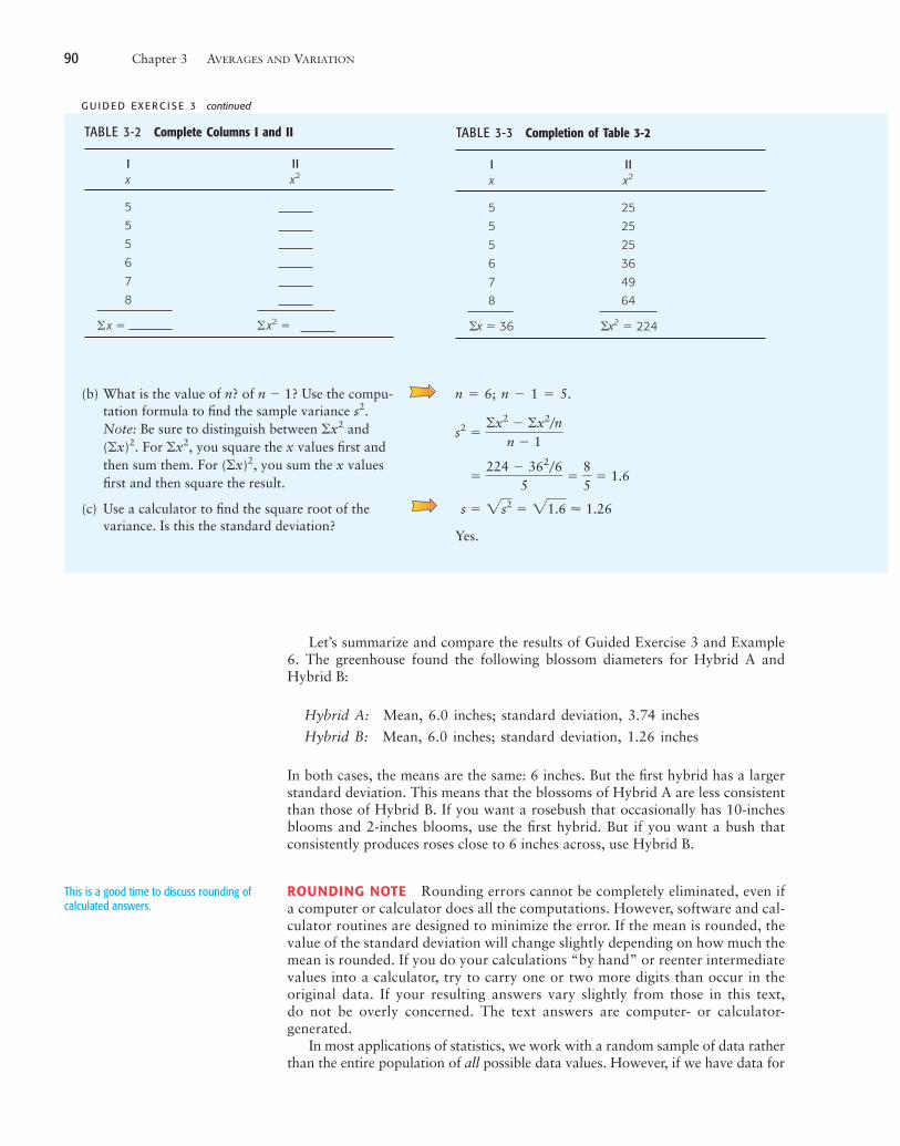
(b) What is the value of n? of n $ 1? Use the compu-tation formula to find the sample variance s2.Note: Be sure to distinguish between and

For , you square the x values first andthen sum them. For you sum the x valuesfirst and then square the result.

(c) Use a calculator to find the square root of thevariance. Is this the standard deviation?

n ! 6; n $ 1 ! 5.

Yes.

s ! 2s2 ! 21.6 " 1.26

!224 $ 362%6

5!

85

! 1.6

s2 !!x2 $ !x2%n

n $ 1

(!x)2,!x2(!x)2.

!x2

TABLE 3-2 Complete Columns I and II

I IIx x2

555678

! x ! ! x2 !

TABLE 3-3 Completion of Table 3-2

I IIx x2

5 255 255 256 367 498 64

!x2 ! 224!x ! 36

1020437_Ch03_p074-121 7/13/07 4:55 AM Page 90

the entire population, we can compute the population mean m, population variances2, and population standard deviation s (lowercase Greek letter sigma) using thefollowing formulas:

Population Parameters

where N is the number of data values in the population and x represents theindividual data values of the population.

We note that the formula for m is the same as the formula for (the sample mean)and the formulas for s2 and s are the same as those for s2 and s (sample varianceand sample standard deviation), except that the population size N is used insteadof n $ 1. Also, m is used instead of in the formulas for s2 and s.

In the formulas for s and s we use n $ 1 to compute s, and N to compute s.Why? The reason is that N (capital letter) represents the population size,whereas n (lowercase letter) represents the sample size. Since a random sam-ple usually will not contain extreme data values (large or small), we divide byn $ 1 in the formula for s to make s a little larger than it would have been hadwe divided by n. Courses in advanced theoretical statistics show that this proce-dure will give us the best possible estimate for the standard deviation s. In fact,s is called the unbiased estimate for s. If we have the population of all data val-ues, then extreme data values are, of course, present, so we divide by N insteadof N $ 1.

COMMENT The computation formula for the population standard deviation is

We’ve seen that the standard deviation (sample or population) is a measure ofdata spread. We will use the standard deviation extensively in later chapters.

s ! v!x2 $ 1!x22%NN

x

x

Population standard deviation ! s ! v!1x $ m22N

Population variance ! s2 !!(x $ m)2

N

Population mean ! m !!xN


This is a good time once again to stress thedifference between sample data andpopulation data. It is interesting to note thatthe concept of population variance s2 wasborrowed from classical mechanics. If youcheck a college physics textbook, you willfind that the formula for s2 is essentiallythe same formula physicists use for thesecond moment.

Population mean variance andstandard deviation

TECH NOTE Most scientific or business calculators have a statistics mode and provide the meanand sample standard deviation directly. The TI-84Plus/TI-83Plus calculators, Excel,and Minitab provide the median and several other measures as well.

Many technologies display only the sample standard deviation s. You can quicklycompute s if you know s by using the formula

The mean given in displays can be interpreted as the sample mean or the populationmean m as appropriate.

The following three displays show output for the hybrid rose data of GuidedExercise 3.

TI-84Plus/TI-83Plus Display Press STAT ➤ CALC ➤ 1:1-Var Stats. Sx is the sample stan-dard deviation. sx is the population standard deviation.

x

s ! svn $ 1n

In Chapter 6 we will use the standarddeviation to study standard z values andareas under normal curves. In Chapters 8and 9 we will use it to study the inferentialstatistics topics of estimation and testing.The standard deviation will appear again inour study of regression and correlation.

1020437_Ch03_p074-121 7/13/07 4:55 AM Page 91

Excel Display Menu choices: Tools ➤ Data Analysis ➤ Descriptive Statistics. Check thesummary statistics box. The standard deviation is the sample standard deviation.

Minitab Display Menu choices: Stat ➤ Basic Statistics ➤ Display Descriptive Statistics.StDev is the sample standard deviation. TrMean is a 5% trimmed mean.

N Mean Median TrMean StDev SE Mean6 6.000 5.500 6.000 1.265 0.516Minimum Maximum Q1 Q35.000 8.000 5.000 7.250

MeanStandard ErrorMedianModeStandard DeviationSample VarianceKurtosisSkewnessRangeMinimumMaximumSumCount

Column 1

60.516398

5.55

1.2649111.6

–0.781250.889391

358

366


Now let’s look at two immediate applications of the standard deviation. The firstis the coefficient of variation, and the second is Chebyshev’s theorem.

Coefficient of VariationA disadvantage of the standard deviation as a comparative measure of varia-tion is that it depends on the units of measurement. This means that it is diffi-cult to use the standard deviation to compare measurements from differentpopulations. For this reason, statisticians have defined the coefficient of varia-tion, which expresses the standard deviation as a percentage of the sample orpopulation mean.

If and s represent the sample mean and sample standard deviation, respec-tively, then the sample coefficient of variation CV is defined to be

CV !sx

! 100

xA good class discussion topic about CV canbe found in Linking Concepts, Problem 3(robin eggs and elephants). See also DataHighlights, Problem 1 (Old Faithful).

Coefficient of variation

1020437_Ch03_p074-121 7/13/07 4:55 AM Page 92

If m and s represent the population mean and population standard deviation,respectively, then the population coefficient of variation CV is defined to be

Notice that the numerator and denominator in the definition of CV have thesame units, so CV itself has no units of measurement. This gives us the advantageof being able to directly compare the variability of two different populationsusing the coefficient of variation.

In the next example and guided exercise, we will compute the CV of a popu-lation and of a sample and then compare the results.

CV !s

m! 100


EXAMPLE 7 Coefficient of variationThe Trading Post on Grand Mesa is a small, family-run store in a remote part ofColorado. The Grand Mesa region contains many good fishing lakes, so theTrading Post sells spinners (a type of fishing lure). The store has a very limitedselection of spinners. In fact, the Trading Post has only eight different types ofspinners for sale. The prices (in dollars) are

2.10 1.95 2.60 2.00 1.85 2.25 2.15 2.25

Since the Trading Post has only eight different kinds of spinners for sale, we con-sider the eight data values to be the population.

(a) Use a calculator with appropriate statistics keys to verify that for the TradingPost data, m " $2.14 and s " $0.22.

SOLUTION: Since the computation formulas for and m are identical, most cal-culators provide the value of only. Use the output of this key for m. Thecomputation formulas for the sample standard deviation s and the populationstandard deviation s are slightly different. Be sure that you use the key for s(sometimes designated as sn or sx).

(b) Compute the CV of prices for the Trading Post and comment on the meaningof the result.

SOLUTION:

The coefficient of variation can be thought of as a measure of the spread ofthe data relative to the average of the data. Since the Trading Post is verysmall, it carries a small selection of spinners that are all priced similarly. TheCV tells us that the standard deviation of the spinner prices is only 10.28%of the mean.

CV !s

m& 100 !

0.222.14

& 100 ! 10.28%

xx

G U I D E D E X E R C I S E 4 Coefficient of variationCabela’s in Sidney, Nebraska, is a very large outfitter that carries a broad selection of fishing tackle.It markets its products nationwide through a catalog service. A random sample of 10 spinners fromCabela’s extensive spring catalog gave the following prices (in dollars):

1.69 1.49 3.09 1.79 1.39 2.89 1.49 1.39 1.49 1.99

Continue

1020437_Ch03_p074-121 7/13/07 4:55 AM Page 93

Chebyshev’s TheoremFrom our earlier discussion about standard deviation, we recall that the spread ordispersion of a set of data about the mean will be small if the standard deviationis small, and it will be large if the standard deviation is large. If we are dealingwith a symmetrical bell-shaped distribution, then we can make very definite state-ments about the proportion of the data that must lie within a certain number ofstandard deviations on either side of the mean. This will be discussed in detail inChapter 6 when we talk about normal distributions.

However, the concept of data spread about the mean can be expressed quitegenerally for all data distributions (skewed, symmetric, or other shape) by usingthe remarkable theorem of Chebyshev.

Chebyshev’s theorem

For any set of data (either population or sample) and for any constant kgreater than 1, the proportion of the data that must lie within k standarddeviations on either side of the mean is at least

Results of Chebyshev’s theorem

For any set of data:

• at least 75% of the data fall in the interval from m $ 2s to m " 2s.

• at least 88.9% of the data fall in the interval from m $ 3s to m " 3s.

• at least 93.8% of the data fall in the interval from m $ 4s to m " 4s.

The results of Chebyshev’s theorem can be derived by using the theorem anda little arithmetic. For instance, if we create an interval k ! 2 standard deviationson either side of the mean, Chebyshev’s theorem tells us that

is the minimum percentage of data in the m $ 2s to m " 2m interval.

1 $1

22! 1 $

14

!34

or 75%

1 $1

k2


(a) Use a calculator with sample mean and samplestandard deviation keys to compute and s.

(b) Compute the CV for the spinner prices atCabela’s.

(c) Compare the mean, standard deviation, and CVfor the spinner prices at the Grand Mesa TradingPost (Example 7) and Cabela’s. Comment on thedifferences.

and s " $0.62.

CV !sx

& 100 !0.621.87

& 100 ! 33.16%

x ! $1.87x


The CV for Cabela’s is more than three times theCV for the Trading Post. Why? First, because ofthe remote location, the Trading Post tends to havesomewhat higher prices (larger m). Second, theTrading Post is very small, so it has a ratherlimited selection of spinners with a smallervariation in price.

Chebyshev’s theorem is a little abstract andmay require some extra class time. Stressthe completely general nature ofChebyshev’s theorem. A good classdiscussion topic can be found in LinkingConcepts, Problem 4 (butterflies and theorbits of the planets).

1020437_Ch03_p074-121 7/13/07 4:55 AM Page 94

Notice that Chebyshev’s theorem refers to the minimum percentage of datathat must fall within the specified number of standard deviations of the mean. Ifthe distribution is mound-shaped, an even greater percentage of data will fall intothe specified intervals (see the Empirical Rule in Section 6.1).


EXAMPLE 8 Chebyshev’s theoremStudents Who Care is a student volunteer program in which college studentsdonate work time to various community projects such as planting trees.Professor Gill is the faculty sponsor for this student volunteer program. Forseveral years, Dr. Gill has kept a careful record of x ! total number of workhours volunteered by a student in the program each semester. For a randomsample of students in the program, the mean number of hours was ! 29.1hours each semester, with a standard deviation of s ! 1.7 hours each semester.Find an interval A to B for the number of hours volunteered into which at least75% of the students in this program would fit.

SOLUTION: According to results of Chebyshev’s theorem, at least 75% of thedata must fall within 2 standard deviations of the mean. Because the mean is

! 29.1 and the standard deviation is s ! 1.7, the interval is

25.7 to 32.5

At least 75% of the students would fit into the group that volunteered from 25.7to 32.5 hours each semester.

29.1 $ 211.72 to 29.1 " 211.72x $ 2s to x " 2s

x

x

G U I D E D E X E R C I S E 5 Chebyshev interval

Determine a Chebyshev interval about the mean inwhich at least 88.9% of the data fall.

By Chebyshev’s theorem, at least 88.9% of the datafall into the interval

to

Because and s ! 30, the interval is

or from 435 to 615 responses per ad.

525 $ 31302 to 525 " 31302x ! 525

x " 3sx $ 3s

The East Coast Independent News periodically runs ads in its own classified section offering amonth’s free subscription to those who respond. In this way, management can get a sense aboutthe number of subscribers who read the classified section each day. Over a period of 2 years,careful records have been kept. The mean number of responses per ad is with standarddeviation s ! 30.

x ! 525

CRITICALTHINKING

Averages such as the mean are often referred to in the media. However, an aver-age by itself does not tell much about the way data are distributed about themean. Knowledge about the standard deviation or variance, along with the mean,gives a much better picture of the data distribution.

1020437_Ch03_p074-121 7/13/07 4:55 AM Page 95


VIEWPOINT Socially Responsible Investing

Make a difference and make money! Socially responsible mutual funds tend to

screen out corporations that sell tobacco, weapons, and alcohol, as well as companies that are

environmentally unfriendly. In addition, these funds screen out companies that use child labor in

sweatshops. There are 68 socially responsible funds tracked by the Social Investment Forum. For more

information, visit the Brase/Brase statistics site at http://math.college.hmco.com/students and find the link

to social investing.

How do these funds rate compared to other funds? One way to answer this question is to study the

annual percent returns of the funds using both the mean and standard deviation. (See Problem 14 of

this section.)


1. Statistical Literacy Which average, mean, median, or mode, is associated withthe standard deviation?

2. Statistical Literacy What is the relationship between the variance and the stan-dard deviation for a sample data set?

3. Statistical Literacy When computing the standard deviation, does it matterwhether the data are sample data or data comprising the entire population?Explain.

4. Statistical Literacy What symbol is used for the standard deviation when it is asample statistic? What symbol is used for the standard deviation when it is apopulation parameter?

5. Critical Thinking Each of the following data sets has a mean of x– ! 10.

(i) 8 9 10 11 12 (ii) 7 9 10 11 12 (iii) 7 8 10 11 12

(a) Without doing any computations, order the data sets according to increasingvalue of standard deviations.

(b) Why do you expect the difference in standard deviations between data sets(i) and (ii) to be greater than the difference in standard deviations betweendata sets (ii) and (iii)? Hint: Consider how much the data in the respectivesets differ from the mean.

6. Critical Thinking: Data Transformation In this problem, we explore the effecton the standard deviation of adding the same constant to each data value in adata set. Consider the data set 5, 9, 10, 11, 15.(a) Use the defining formula, the computation formula, or a calculator to

compute s.(b) Add 5 to each data value to get the new data set 10, 14, 15, 16, 20.

Compute s.


1. Mean.2. The standard deviation s is the square

root of the variance s2.3. Yes. For the sample standard deviation s,

the sum ∑(x $ )2 is divided by n $ 1,where n is the sample size. For thepopulation standard deviation s, thesum ∑(x $ m)2 is divided by N, whereN is the population size.

4. Sample statistic: s. Populationparameter: s.

5. (a) (i), (ii), (iii).(b) The data change between data sets

(i) and (ii) increased the squareddifference (x $ )2 by 9, whereasthe data change between data sets(ii) and (iii) increased the squareddifference (x $ )2 by only 4.

6. (a) s " 3.6.(b) s " 3.6.

x

x

x

Chebyshev’s theorem tells us that no matter what the data distribution lookslike, at least 75% of the data will fall within 2 standard deviations of the mean.As we will see in Chapter 6, when the distribution is mound-shaped and symmet-ric, about 95% of the data are within 2 standard deviations of the mean. Datavalues beyond 2 standard deviations from the mean are less common than thosecloser to the mean.

In fact, one indicator that a data value might be an outlier is that it is morethan 2.5 standard deviations from the mean (Oxford Dictionary of Statistics,Oxford University Press).

1020437_Ch03_p074-121 7/13/07 4:55 AM Page 96

(c) Compare the results of parts (a) and (b). In general, how do you think thestandard deviation of a data set changes if the same constant is added toeach data value?

7. Critical Thinking: Data Transformation In this problem, we explore the effecton the standard deviation of multiplying each data value in a data set by thesame constant. Consider the data set 5, 9, 10, 11, 15.(a) Use the defining formula, the computation formula, or a calculator to com-

pute s.(b) Multiply each data value by 5 to obtain the data new set 25, 45, 50, 55, 75.

Compute s.(c) Compare the results of parts (a) and (b). In general, how does the standard

deviation change if each data value is multiplied by a constant c?(d) You recorded the weekly distances you bicycled in miles and computed the

standard deviation to be s ! 3.1 miles. Your friend wants to know the stan-dard deviation in kilometers. Do you need to redo all the calculations?Given 1 mile " 1.6 kilometers, what is the standard deviation in kilometers?

8. Critical Thinking: Outliers One indicator of an outlier is that an observation ismore than 2.5 standard deviations from the mean. Consider the data value 80.(a) If a data set has mean 70 and standard deviation 5, is 80 a suspect outlier?(b) If a data set has mean 70 and standard deviation 3, is 80 a suspect outlier?

9. General Concepts: Variance, Standard Deviation Given the sample data

x: 23 17 15 30 25

(a) Find the range.(b) Verify that and (c) Use the results of part (b) and appropriate computation formulas to com-

pute the sample variance s2 and sample standard deviation s.(d) Use the defining formulas to compute the sample variance s2 and sample

standard deviation s.(e) Suppose the given data comprise the entire population of all x values.

Compute the population variance and population standard deviation

10. Investing: Stocks and Bonds Do bonds reduce the overall risk of an investmentportfolio? Let x be a random variable representing annual percent return forVanguard Total Stock Index (all stocks). Let y be a random variable representingannual return for Vanguard Balanced Index (60% stock and 40% bond). For thepast several years, we have the following data (Reference: Morningstar ResearchGroup, Chicago).

x: 11 0 36 21 31 23 24 $11 $11 $21

y: 10 $2 29 14 22 18 14 $2 $3 $10

(a) Compute and (b) Use the results of part (a) to compute the sample mean, variance, and stan-

dard deviation for x and for y.(c) Compute a 75% Chebyshev interval around the mean for x values and also

for y values. Use the intervals to compare the two funds.(d) Compute the coefficient of variation for each fund. Use the coefficients of

variation to compare the two funds. If s represents risks and representsexpected return, then can be thought of as a measure of risk per unit ofexpected return. In this case, why is a smaller CV better? Explain.

11. Space Shuttle: Epoxy Kevlar epoxy is a material used on the NASA SpaceShuttle. Strands of this epoxy were tested at the 90% breaking strength. The fol-lowing data represent time to failure (in hours) for a random sample of 50 epoxystrands (Reference: R. E. Barlow, University of California, Berkeley). Let x be arandom variable representing time to failure (in hours) at 90% breaking

s% xx

!y2.!y,! x2,! x,

s.s2

! x2 ! 2568.! x ! 110


(c) In general, adding a constant c toeach data value in a set does notchange the standard deviation. Thedistribution shifts by c units but thespread between data values doesnot change.

7. (a) s " 3.6.(b) s " 18.0.(c) When each data value is multiplied

by 5, the standard deviation is fivetimes greater than that of the originaldata set. In general, multiplying eachdata value by the same constant cresults in the standard deviationbeing |c| times as large.

(d) No. Multiply 3.1 miles by 1.6kilometers/mile to obtain s " 4.96kilometers.

8. (a) No.(b) Yes, since 80 is more than 2.5

standard deviations above themean.

10. (a) ∑x ! 103; ∑x2 ! 4607; ∑y ! 90; ∑y2 ! 2258.

(b) For total stock: ! 10.3; s2 " 394.0; s "

19.85.For balanced: y– ! 9; s2 " 160.8; s " 12.68.

(c) For total stock x, $29.4 to 50; forbalanced y, $16.36 to 34.36; 75%of the returns for the balanced fundfall within a narrower range thanthose of the stock fund. Inparticular, the low returns for thebalanced fund are not as low asthose of the stock fund. However,the stock fund returns range tohigher values than the balancedfund returns.

(d) For the stock fund, CV " 192.7%; forthe balanced fund, CV " 140.9%.For each unit of return, the balanced

x

9. (a) 15.(b) Use a calculator.(c) 37; 6.08.(d) 37; 6.08.(e) s2 " 29.59; s " 5.44.

11. (a) 7.87.(b) Use a calculator.(c) " 1.24; s2 " 1.78; s " 1.33.

(d) CV " 107%. The standarddeviation of the time to failure isjust slightly larger than the average

x

1020437_Ch03_p074-121 7/13/07 4:55 AM Page 97

strength. Note: These data are also available with other software on thestatSpace CD-ROM.

0.54 1.80 1.52 2.05 1.03 1.18 0.80 1.33 1.29 1.11

3.34 1.54 0.08 0.12 0.60 0.72 0.92 1.05 1.43 3.03

1.81 2.17 0.63 0.56 0.03 0.09 0.18 0.34 1.51 1.45

1.52 0.19 1.55 0.02 0.07 0.65 0.40 0.24 1.51 1.45

1.60 1.80 4.69 0.08 7.89 1.58 1.64 0.03 0.23 0.72

(a) Find the range.(b) Use a calculator to verify that and (c) Use the results of part (b) to compute the sample mean, variance, and stan-

dard deviation for the time to failure.(d) Use the results of part (c) to compute the coefficient of variation. What does

this number say about time to failure? Why does a small CV indicate moreconsistent data, whereas a larger CV indicates less consistent data? Explain.

12. Archaeology: Ireland The Hill of Tara in Ireland is a place of great archaeolog-ical importance. This region has been occupied by people for more than 4,000years. Geomagnetic surveys detect subsurface anomalies in the earth’s magneticfield. These surveys have led to many significant archaeological discoveries.After collecting data, the next step is to begin a statistical study. The followingdata measure magnetic susceptibility (centimeter-gram-second & 10$6) on twoof the main grids of the Hill of Tara (Reference: Tara: An Archaeological Surveyby Conor Newman, Royal Irish Academy, Dublin).

Grid E: x variable

13.20 5.60 19.80 15.05 21.40 17.25 27.45

16.95 23.90 32.40 40.75 5.10 17.75 28.35

Grid H: y variable

11.85 15.25 21.30 17.30 27.50 10.35 14.90

48.70 25.40 25.95 57.60 34.35 38.80 41.00

31.25

(a) Compute and (b) Use the results of part (a) to compute the sample mean, variance, and stan-

dard deviation for x and for y.(c) Compute a 75% Chebyshev interval around the mean for x values and also

for y values. Use the intervals to compare the magnetic susceptibility on thetwo grids. Higher numbers indicate higher magnetic susceptibility. However,extreme values, high or low, could mean an anomaly and possible archaeo-logical treasure.

(d) Compute the sample coefficient of variation for each grid. Use the CV’s tocompare the two grids. If s represents variability in the signal (magnetic sus-ceptibility) and represents the expected level of the signal, then can bethought of as a measure of the variability per unit of expected signal.Remember, a considerable variability in the signal (above or below average)might indicate buried artifacts. Why, in this case, would a large CV be better,or at least more exciting? Explain.

13. Wildlife: Mallard Ducks and Canada Geese For mallard ducks and Canadageese, what percentage of nests are successful (at least one offspring survives)?Studies in Montana, Illinois, Wyoming, Utah, and California gave the follow-

s% xx

!y2.!y,!x2,!x,

! x2 " 164.23.! x ! 62.11


12. (a) ∑x ! 284.95; ∑x2 " 7046.80; ∑y ! 421.5; ∑y2 " 14,562.29.

(b) For Grid E, " 20.35; s2 " 96; s " 9.79; for Grid H,

! 28.1; s2 " 194; s " 13.93.

(c) For Grid E, 0.77 to 39.93; for Grid H,0.24 to 55.96. Grid H shows a wider75% range of values.

(d) For Grid E, CV " 48%; for Grid H,CV " 50%. Grid H demonstratesslightly greater variability perexpected signal. The CV, togetherwith the confidence interval,indicates that Grid H might havemore buried artifacts.

yx

1020437_Ch03_p074-121 7/13/07 4:55 AM Page 98

ing percentages of successful nests (Reference: The Wildlife Society Press,Washington, D.C.).

x: Percentage success for mallard duck nests

56 85 52 13 39

y: Percentage success for Canada goose nests

24 53 60 69 18

(a) Use a calculator to verify that and

(b) Use the results of part (a) to compute the sample mean, variance, and stan-dard deviation for x, the percent of successful mallard nests.

(c) Use the results of part (a) to compute the sample mean, variance, and stan-dard deviation for y, the percent of successful Canada goose nests.

(d) Use the results of parts (b) and (c) to compute the coefficient of variation forsuccessful mallard nests and Canada goose nests. Write a brief explanationof the meaning of these numbers. What do these results say about the nest-ing success rates for mallards compared to Canada geese? Would you sayone group of data is more or less consistent than the other? Explain.

14. Investing: Socially Responsible Mutual Funds Pax World Balanced is a highlyrespected, socially responsible mutual fund of stocks and bonds (see Viewpoint).Vanguard Balanced Index is another highly regarded fund that represents theentire U.S. stock and bond market (an index fund). The mean and standard devi-ation of annualized percent returns are shown below. The annualized meanand standard deviation are based on the years 1993 through 2002 (Source:Morningstar).

Pax World Balanced: ! 9.58%; s ! 14.05%Vanguard Balanced Index: ! 9.02%; s ! 12.50%

(a) Compute the coefficient of variation for each fund. If represents return ands represents risk, then explain why the coefficient of variation can be takento represent risk per unit of return. From this point of view, which fundappears to be better? Explain.

(b) Compute a 75% Chebyshev interval around the mean for each fund. Use theintervals to compare the two funds. As usual, past performance does notguarantee future performance.

15. Medical: Physician Visits In some reports, the mean and coefficient of variationare given. For instance, in Statistical Abstract of the United States, 116thEdition, one report gives the average number of physician visits by males peryear. The average reported is 2.2, and the reported coefficient of variation is1.5%. Use this information to determine the standard deviation of the annualnumber of visits to physicians made by males.

x

xx

12,070.!y2 !

!y ! 224;!x2 ! 14,755;!x ! 245;


Expand Your Knowledge: Grouped data

When data are grouped, such as in a frequency table or histogram, we canestimate the mean and standard deviation by using the following formulas.Notice that all data values in a given class are treated as though each ofthem equals the midpoint x of the class.

Sample mean for a frequency distribution

(5)x !!xfn

Grouped data

Approximating x– and s fromgrouped data

13. (a) Use a calculator.(b) ! 49; s2 " 687.49; s " 26.22.

(c) ! 44.8; s2 " 508.50; s "22.55.

(d) Mallard nest CV " 53.5%; Canadagoose nest CV " 50.3%. The CVgives the ratio of the standarddeviation to the mean; the CV for

yx

14. (a) Pax, CV " 146.7%; Vanguard, CV " 138.6%. Vanguard fund hasslightly less risk per unit of return.

(b) Pax, $18.52% to 37.68%; Vanguard,$15.98% to 34.02%. Vanguard hasa narrower range of returns, withless downside, but also less upside.

15. Since CV ! s/ , then s ! CV (x–). s ! 0.033.

x

1020437_Ch03_p074-121 7/13/07 4:55 AM Page 99

Sample standard deviation for a frequency distribution

(6)

Computation formula for the sample standard deviation

(7)

where

x is the midpoint of a class,

f is the number of entries in that class,

n is the total number of entries in the distribution, and n ! !f.

The summation ! is over all classes in the distribution.

s ! v!x2f $ 1!xf 22%nn $ 1

s ! v!1x $ x22fn $ 1


Use formulas (5) and (6) or (5) and (7) to solve Problems 16–19. To use formulas (5)and (6) to evaluate the sample mean and standard deviation, use the followingcolumn heads:

Midpoint x Frequency f xf

For formulas (5) and (7), use these column heads:

Midpoint x Frequency f xf

Note: On the TI-83 calculator, enter the midpoints in column L1 and the frequenciesin column L2. Then use 1-VarStats L1, L2.

16. Anthropology: Navajo Reservation What was the age distribution of prehis-toric Native Americans? Extensive anthropologic studies in the southwesternUnited States gave the following information about a prehistoric extendedfamily group of 80 members on what is now the Navajo Reservation in north-western New Mexico. (Source: Based on information taken from Prehistory inthe Navajo Reservation District, by F. W. Eddy, Museum of New MexicoPress.)

Age range (years) 1–10* 11–20 21–30 31 and overNumber of individuals 34 18 17 11

*Includes infants.

For this community, estimate the mean age expressed in years, the sample vari-ance, and the sample standard deviation. For the class 31 and over, use 35.5 asthe class midpoint.

17. Crime: Shoplifting What is the age distribution of adult shoplifters (21 years ofage or older) in supermarkets? The following is based on information takenfrom the National Retail Federation. A random sample of 895 incidents ofshoplifting gave the following age distribution:

Age range (years) 21–30 31–40 41 and overNumber of shoplifters 260 348 287

Estimate the mean age, sample variance, and sample standard deviation for theshoplifters. For the class 41 and over, use 45.5 as the class midpoint.

x2 fx2

(x $ x)2 f(x $ x)2(x $ x)

Sometimes grouped data are the only datawe can get our hands on. In othersituations, it is easier first to group the dataand then to estimate the mean andstandard deviation.

16. " 16.1; s2 " 119.9; s " 10.95.x

17. " 35.8; s2 " 61.1; s " 7.82.x

1020437_Ch03_p074-121 7/13/07 4:55 AM Page 100

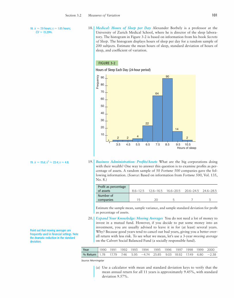
18. Medical: Hours of Sleep per Day Alexander Borbely is a professor at theUniversity of Zurich Medical School, where he is director of the sleep labora-tory. The histogram in Figure 3-2 is based on information from his book Secretsof Sleep. The histogram displays hours of sleep per day for a random sample of200 subjects. Estimate the mean hours of sleep, standard deviation of hours ofsleep, and coefficient of variation.

19. Business Administration: Profits/Assets What are the big corporations doingwith their wealth? One way to answer this question is to examine profits as per-centage of assets. A random sample of 50 Fortune 500 companies gave the fol-lowing information. (Source: Based on information from Fortune 500, Vol. 135,No. 8.)

Profit as percentage of assets 8.6–12.5 12.6–16.5 16.6–20.5 20.6–24.5 24.6–28.5Number of companies 15 20 5 7 3

Estimate the sample mean, sample variance, and sample standard deviation for profitas percentage of assets.

20. Expand Your Knowledge: Moving Averages You do not need a lot of money toinvest in a mutual fund. However, if you decide to put some money into aninvestment, you are usually advised to leave it in for (at least) several years.Why? Because good years tend to cancel out bad years, giving you a better over-all return with less risk. To see what we mean, let’s use a 3-year moving averageon the Calvert Social Balanced Fund (a socially responsible fund).


Hours of Sleep Each Day (24-hour period)

FIGURE 3-2

3.5

2 2 2

90

80

70

60

50

40

30

20

10

Freq

uenc

y

Hours of sleep4.5 5.5

4

6.5

22

7.5 8.5

64

90

9.5

14

10.5

Point out that moving averages arefrequently used in financial settings. Notethe dramatic reduction in the standarddeviation.

Year 1990 1991 1992 1993 1994 1995 1996 1997 1998 1999 2000% Return 1.78 17.79 7.46 5.95 $4.74 25.85 9.03 18.92 17.49 6.80 $2.38

(a) Use a calculator with mean and standard deviation keys to verify that themean annual return for all 11 years is approximately 9.45%, with standarddeviation 9.57%.

18. " 7.9 hours; s " 1.05 hours; CV " 13.29%.

x

Source: Morningstar

19. " 15.6; s2 " 23.4; s " 4.8.x

1020437_Ch03_p074-121 7/13/07 4:55 AM Page 101

(b) To compute a 3-year moving average for 1992, we take the data values for1992 and the prior two years and average them. To compute a 3-year mov-ing average for 1993, we take the data values for 1993 and the prior twoyears and average them. Verify that the following 3-year moving averagesare correct.

(c) Use a calculator with mean and standard deviation keys to verify that for the3-year moving average, the mean is 10.68% with sample standard deviation4.53%.

(d) Compare the results of parts (a) and (c). Suppose we take the point of viewthat risk is measured by standard deviation. Is the risk (standard deviation)of the 3-year moving average considerably smaller? This is an example of ageneral phenomenon that will be studied in more detail in Chapter 6.

21. Brain Teaser: Sum of Squares If you like mathematical puzzles or love algebra,try this! Otherwise, just trust that the computational formula for the sum ofsquares is correct. We have a sample of x values. The sample size is n. Fill in thedetails for the following steps.

! !x2 $1!x22

n

! !x2 $ 2nx 2 " nx

2

!1x $ x 22 ! !x2 $ 2 x !x " nx 2


Year 1992 1993 1994 1995 1996 1997 1998 1999 20003-year moving average 9.01 10.40 2.89 9.02 10.05 17.93 15.15 14.40 7.30

20. (d) The 3-year moving average has amuch lower standard deviation.

S EC T I O N 3 . 3 Percentiles and Box-and-Whisker PlotsFOCUS POINTS

• Interpret the meaning of percentile scores.• Compute the median, quartiles, and five-number summary from raw data.• Make a box-and-whisker plot. Interpret the results.• Describe how a box-and-whisker plot indicates spread of data about the median.

We’ve seen measures of central tendency and spread for a set of data. The arith-metic mean and the standard deviation s will be very useful in later work.However, because they each utilize every data value, they can be heavily influ-enced by one or two extreme data values. In cases where our data distributionsare heavily skewed or even bimodal, we often get a better summary of the distri-bution by utilizing relative position of data rather than exact values.

Recall that the median is an average computed by using relative position ofthe data. If we are told that 81 is the median score on a biology test, we knowthat after the data have been ordered, 50% of the data fall at or below themedian value of 81. The median is an example of a percentile; in fact, it is the50th percentile. The general definition of the Pth percentile follows.

For whole numbers P (where 1 # P # 99), the Pth percentile of a distribution isa value such that P% of the data fall at or below it and (100 $ P)% of the datafall at or above it.

In Figure 3-3, we see the 60th percentile marked on a histogram. We see that60% of the data lie below the mark and 40% lie above it.

x

This is a conceptually important section onwhich it is worth spending a little extra timein class discussion. See Linking Conceptsand Using Technology.

Percentile

1020437_Ch03_p074-121 7/13/07 4:55 AM Page 102

Section 3.3 Percentiles and Box-and-Whisker Plots 103

A Histogram with the 60th Percentile Shown

FIGURE 3-3

Percentiles

FIGURE 3-4

Lowest Highest1st1%

2nd 3rd 4th 5th…

99th98thPercentiles

1% 1% 1% 1% 1% 1% 1%

G U I D E D E X E R C I S E 6 Percentiles

(a) If your score is at the 89th percentile, whatpercentage of scores are at or below yours?

(b) If the scores ranged from 1 to 100 and your raw score is 95, does this necessarily mean that your score is at the 95th percentile?

You took the English achievement test to obtain college credit in freshman English byexamination.

The percentile means that 89% of the scores are at orbelow yours.

No, the percentile gives an indication of relativeposition of the scores. The determination of yourpercentile has to do with the number of scores at orbelow yours. If everyone did very well and only 80%of the scores fell at or below yours, you would be atthe 80th percentile even though you got 95 out of 100points on the exam.

There are 99 percentiles, and in an ideal situation, the 99 percentiles dividethe data set into 100 equal parts. (See Figure 3-4.) However, if the number of dataelements is not exactly divisible by 100, the percentiles will not divide the datainto equal parts.

There are several widely used conventions for finding percentiles. They lead toslightly different values for different situations, but these values are closetogether. For all conventions, the data are first ranked or ordered from smallest tolargest. A natural way to find the Pth percentile is to then find a value such thatP% of the data fall at or below it. This will not always be possible, so we take thenearest value satisfying the criterion. It is at this point that there are a variety ofprocesses to determine the exact value of the percentile.

1020437_Ch03_p074-121 7/13/07 4:55 AM Page 103

We will not be very concerned about exact procedures for evaluating per-centiles in general. However, quartiles are special percentiles used so frequentlythat we want to adopt a specific procedure for their computation.

Quartiles are those percentiles that divide the data into fourths. The firstquartile Q1 is the 25th percentile, the second quartile Q2 is the median, and thethird quartile Q3 is the 75th percentile. (See Figure 3-5.)

Again, several conventions are used for computing quartiles, but the follow-ing convention utilizes the median and is widely adopted.


Quartiles

FIGURE 3-5

PROCEDURE HOW TO COMPUTE QUARTILES


2. Find the median. This is the second quartile.

3. The first quartile Q1 is then the median of the lower half of the data;that is, it is the median of the data falling below the Q2 position (andnot including Q2).

4. The third quartile Q3 is the median of the upper half of the data; that is,it is the median of the data falling above the Q2 position (and notincluding Q2).

In short, all we do to find the quartiles is find three medians.The median, or second quartile, is a popular measure of the center utilizing

relative position. A useful measure of data spread utilizing relative position is theinterquartile range (IQR). It is simply the difference between the third and firstquartiles.

Interquartile range ! Q3 $ Q1

The interquartile range tells us the spread of the middle half of the data. Now let’slook at an example to see how to compute all of these quantities.

It is helpful to remind students that themedian itself does not fall into either thelower or upper half of the data. In the caseof an even number of data, however, thetwo values used to compute the medianare included in the lower and upper halvesof the data, respectively.

EXAMPLE 9 QuartilesIn a hurry? On the run? Hungry as well? How about an ice cream bar as a snack?Ice cream bars are popular among all age groups. Consumer Reports did a studyof ice cream bars. Twenty-seven bars with taste ratings of at least “fair” werelisted, and cost per bar was included in the report. Just how much will an icecream bar cost? The data, expressed in dollars, appear in Table 3-4. As you cansee, the cost varies quite a bit, partly because the bars are not of uniform size.

1020437_Ch03_p074-121 7/13/07 4:55 AM Page 104

(a) Find the quartiles.

SOLUTION: We first order the data from smallest to largest. Table 3-5 showsthe data in order. Next, we find the median. Since the number of data valuesis 27, there are an odd number of data, and the median is simply the center or14th value. The value is shown boxed in Table 3-5.

Median ! Q2 ! 0.50

There are 13 values below the median position, and Q1 is the median of these val-ues. It is the middle or seventh value and is shaded in Table 3-5.

First quartile ! Q1 ! 0.33

There are also 13 values above the median position. The median of these isthe seventh value from the right end. This value is also shaded in Table 3-5.

Third quartile ! Q3 ! 1.00

(b) Find the interquartile range.

SOLUTION:IQR ! Q3 $ Q1

! 1.00 $ 0.33

! 0.67

This means that the middle half of the data has a cost spread of 67¢.

(b) The experiment involved two plots at each station. The plot that was notfenced represents the control plot. This is the plot on which a


TABLE 3-4 Cost of Ice Cream Bars (in dollars)0.99 1.07 1.00 0.50 0.37 1.03 1.07 1.070.97 0.63 0.33 0.50 0.97 1.08 0.47 0.841.23 0.25 0.50 0.40 0.33 0.35 0.17 0.380.20 0.18 0.16

TABLE 3-5 Ordered Cost of Ice Cream Bars (in dollars)0.16 0.17 0.18 0.20 0.25 0.33 0.33 0.350.37 0.38 0.40 0.47 0.50 0.50 0.50 0.630.84 0.97 0.97 0.99 1.00 1.03 1.07 1.071.07 1.08 1.23

G U I D E D E X E R C I S E 7 QuartilesMany people consider the number of calories in an ice cream bar as important as, if not moreimportant than, the cost. The Consumer Reportsarticle also included the calorie count of the ratedice cream bars (Table 3-6). There were 22 vanilla-flavored bars rated. Again, the bars varied in size,and some of the smaller bars had fewer calories.The calorie counts for the vanilla bars follow.

(a) Our first step is to order the data. Do so.

TABLE 3-6 Calories in Vanilla-Flavored Ice Cream Bars

342 377 319 353 295234 294 286 377 182310 439 111 201 182197 209 147 190 151131 151

TABLE 3-7 Ordered Data

111 131 147 151 151 182182 190 197 201 209 234286 294 295 310 319 342353 377 377 439

Continue

1020437_Ch03_p074-121 7/13/07 4:55 AM Page 105

Box-and-Whisker PlotsThe quartiles together with the low and high data values give us a very usefulfive-number summary of the data and their spread.

Five-number summary

Lowest value, Q1, median, Q3, highest value

We will use these five numbers to create a graphic sketch of the data called abox-and-whisker plot. Box-and-whisker plots provide another useful techniquefrom exploratory data analysis (EDA) for describing data.


(b) There are 22 data values. Find the median. Average the 11th and 12th data values boxedtogether in Table 3-7.

(c) How many values are below the medianposition? Find Q1.

(d) There are the same number of data above asbelow the median. Use this fact to find Q3.

(e) Find the interquartile range and comment on itsmeaning.

Since the median lies halfway between the 11th and12th values, there are 11 values below the medianposition. Q1 is the median of these values.

Q1 ! 182

Q3 is the median of the upper half of the data. Thereare 11 values in the upper portion.

Q3 ! 319

IQR ! Q3 $ Q1

! 319 $ 182

! 137

The middle portion of the data has a spread of 137 calories.


! 221.5

Median !209 " 234

2

Five-number summary

Box-and-whisker plot

A good class discussion topic can be foundin Linking Concepts, Problem 2. Thisproblem compares earlier concepts of thischapter with the box-and-whisker plot. It isgood to emphasize that the box-and-whisker plot is easy to construct andcontains a lot of information at a glance.

PROCEDURE HOW TO MAKE A BOX-AND-WHISKER PLOT

1. Draw a vertical scale to include the lowest and highest data values.

2. To the right of the scale, draw a box from Q1 to Q3.

3. Include a solid line through the box at the median level.

4. Draw vertical lines, called whiskers, from Q1

to the lowest value and from Q3 to the highest value.

Box-and-Whisker Plot

FIGURE 3-6Use the five-number summary and steps 1to 4 for making a box-and-whisker plot as akind of mental flowchart to help studentsorganize their work.

It is helpful to point out that a box-and-whisker plot serves the function of adescription of data spread about themedian, while the standard deviation is ameasure of spread about the mean.

The next example demonstrates the process of making a box-and-whisker plot.

1020437_Ch03_p074-121 7/13/07 4:55 AM Page 106

EXAMPLE 10 Box-and-whisker plotUsing the data from Guided Exercise 7, make a box-and-whisker plot showingthe calories in vanilla-flavored ice cream bars. Use the plot to make observationsabout the distribution of calories.

(a) In Guided Exercise 7, we ordered the data (see Table 3-7) and found the val-ues of the median, Q1, and Q3. From this previous work we have the follow-ing five-number summary:

low value ! 111; Q1 ! 182; median ! 221.5; Q3 ! 319; high value ! 439

(b) We select an appropriate vertical scale and make the plot (Figure 3-7).

(c) A quick glance at the box-and-whisker plot reveals the following:

(i) The box tells us where the middle half of the data lies, so we see that halfof the ice cream bars have between 182 and 319 calories, with aninterquartile range of 137 calories.

(ii) The median is slightly closer to the lower part of the box. This means thatthe lower calorie counts are more concentrated. The calorie counts abovethe median are more spread out, indicating that the distribution is slightlyskewed toward the higher values.

(iii) The upper whisker is longer than the lower, which again emphasizesskewness toward the higher values.


Box-and-Whisker Plot for Calories inVanilla-Flavored Ice Cream Bars

FIGURE 3-7

COMMENT In exploratory data analysis, hinges rather than quartiles areused to create the box. Hinges are computed in a manner similar to themethod used to compute quartiles. However, in the case of an odd number ofdata values, include the median itself in both the lower and upper halves ofthe data (see Applications, Basics, and Computing of Exploratory DataAnalysis, by Paul Velleman and David Hoaglin, Duxbury Press). This has theeffect of shrinking the box and moving the ends of the box slightly toward themedian. For an even number of data, the quartiles as we computed them equalthe hinges.

450

400

350

300

250

200

150

100

Calories

439.0

319.0

221.5182.0

111.0

G U I D E D E X E R C I S E 8 Box-and-whisker plot

(a) From Figure 3-8, estimate the median andextreme values of salaries of alumni graduating 2years ago. In what range are the middle half ofthe salaries?

The Renata College Development Office sent salary surveys to alumni who graduated 2 and 5 yearsago. The voluntary responses received are summarized in the box-and-whisker plots shown inFigure 3-8.

The median seems to be about $44,000. The extremesare about $33,000 and $54,000. The middle half ofthe salaries fall between $40,000 and $47,000.

1020437_Ch03_p074-121 7/13/07 4:55 AM Page 107

CRITICAL THINKING Box-and-whisker plots provide a graphic display of the spread of data about the

median. The box shows the location of the middle half of the data. One quarterof the data are located along each whisker.

To the extent that the median is centered in the box and the whiskers areabout the same length, the data distribution is symmetric around the median. Ifthe median line is near one end of the box, the data are skewed toward the otherside of the box.

We have developed the skeletal box-and-whisker display. Other variationsinclude fences, which are marks placed on either side of the box to represent vari-ous portions of data. Values that lie beyond the fences are outliers. Problem 10 ofthis section discusses some criteria for locating fences and identifying outliers.


(b) From Figure 3-8, estimate the median and theextreme values of salaries of alumni graduating 5 years ago. What is the location of the middlehalf of the salaries?

(c) Compare the two box plots and make commentsabout the salaries of alumni graduating 2 and5 years ago.

The median seems to be $47,000. The extremes are$34,000 and $58,000. The middle half of the dataare enclosed by the box with low side at $41,000and high side at $50,000.

The salaries of the alumni graduating 5 years agohave a larger range. They begin slightly higher thanand extend to levels about $4,000 above the salariesof those graduating 2 years ago. The middle half ofthe data are also more spread out, with higherboundaries and a higher median.


Box-and-Whisker Plots for Alumni Salaries (inthousands of dollars)

FIGURE 3-8

TECH NOTES Box-and-Whisker Plot

Both Minitab and the TI-84Plus/ TI-83Plus calculators support box-and-whiskerplots. On the TI-84Plus/ TI-83Plus, the quartiles Q1 and Q3 are calculated as we cal-culate them in this text. In Minitab and Excel, they are calculated using a slightly dif-ferent process.

TI-84Plus/TI-83Plus Press STATPLOT ➤ On. Highlight box plot. Use Trace and thearrow keys to display the values of the five-number summary. The display shows theplot for calories in ice cream bars.

1020437_Ch03_p074-121 7/13/07 4:55 AM Page 108

Excel Does not produce plot. Paste Function ➤ Statistics ➤ Quartiles gives thefive-number summary.

Minitab Press Graph ➤ Boxplot. In the dialogue box, set Display to IQRange Box.

fx

Med=221.5


VIEWPOINT Is Shorter Higher?

Can you estimate a person’s height from the pitch of his or her voice? Is a

soprano shorter than an alto? Is a bass taller than a tenor? A statistical study of singers in the New York

Choral Society provided information. For more information, visit the Brase/Brase statistics site at

http://math.college.hmco.com/students and find the link to DASL, the Carnegie Mellon University Data

and Story Library. From the Data Subjects, select music and then singers. Methods of this chapter can

be used with new methods we will learn in Chapters 8 and 9 to examine such questions from a

statistical point of view.


1. Statistical Literacy Angela took a general aptitude test and scored in the 82ndpercentile for aptitude in accounting. What percentage of the scores were at orbelow her score? What percentage were above?

2. Statistical Literacy One standard for admission to Redfield College is that thestudent must rank in the upper quartile of his or her graduating high schoolclass. What is the minimal percentile rank of a successful applicant?

3. Critical Thinking The town of Butler, Nebraska, decided to give a teacher-com-petency exam and defined the passing scores to be those in the 70th percentile orhigher. The raw test scores ranged from 0 to 100. Was a raw score of 82 neces-sarily a passing score? Explain.

4. Critical Thinking Clayton and Timothy took different sections of Introductionto Economics. Each section had a different final exam. Timothy scored 83 out of100 and had a percentile rank in his class of 72. Clayton scored 85 out of 100but his percentile rank in his class was 70. Who performed better with respect tothe rest of the students in the class, Clayton or Timothy? Explain your answer.

5. Health Care: Nurses At Center Hospital there is some concern about the highturnover of nurses. A survey was done to determine how long (in months) nurseshad been in their current positions. The responses (in months) of 20 nurses were

23 2 5 14 25 36 27 42 12 8

7 23 29 26 28 11 20 31 8 36

Make a box-and-whisker plot of the data. Find the interquartile range.


1. 82% at or below; 18% above.2. 75th percentile.3. No, it might have a percentile rank less

than 70.

5. Low ! 2; Q1 ! 9.5; median ! 23; Q3 ! 28.5; high ! 42; IQR ! 19.

4. Timothy; Timothy’s percentile score is higher.

1020437_Ch03_p074-121 7/13/07 4:55 AM Page 109

6. Health Care: Staff Another survey was done at Center Hospital to determinehow long (in months) clerical staff had been in their current positions. Theresponses (in months) of 20 clerical staff members were

25 22 7 24 26 31 18 14 17 20

31 42 6 25 22 3 29 32 15 72

(a) Make a box-and-whisker plot. Find the interquartile range.(b) Compare this plot with the one in Problem 5. Discuss the locations of the

medians, the location of the middle halves of the data banks, and the dis-tances from Q1 and Q3 to the extreme values.

7. Sociology: College Graduates What percentage of the general U.S. populationhave bachelor’s degrees? The Statistical Abstract of the United States, 120thEdition, gives the percentage of bachelor’s degrees by state. For convenience, thedata are sorted in increasing order.

17 18 18 18 19 20 20 20 21 21

21 21 22 22 22 22 22 22 23 23

24 24 24 24 24 24 24 24 25 26

26 26 26 26 26 27 27 27 27 27

28 28 29 31 31 32 32 34 35 38

(a) Make a box-and-whisker plot and find the interquartile range.(b) Illinois has a bachelor’s degree percentage rate of about 26%. Into what

quartile does this rate fall?

8. Sociology: High-school Dropouts What percentage of the general U.S. popula-tion are high-school dropouts? The Statistical Abstract of the United States,120th Edition, gives the percentage of high-school dropouts by state. For conven-ience, the data are sorted in increasing order.

5 6 7 7 7 7 8 8 8 8

8 9 9 9 9 9 9 9 10 10

10 10 10 10 10 10 11 11 11 11

11 11 11 11 12 12 12 12 13 13

13 13 13 13 14 14 14 14 14 15

(a) Make a box-and-whisker plot and find the interquartile range.(b) Wyoming has a dropout rate of about 7%. Into what quartile does this

rate fall?

9. Auto Insurance: Interpret Graphs Consumer Reports rated automobile insurancecompanies and gave annual premiums for top-rated companies in several states.Figure 3-9 shows box plots for annual premiums for urban customers (marriedcouple with one 17-year-old son) in three states. The box plots in Figure 3-9 wereall drawn using the same scale on a TI-84Plus/TI-83Plus calculator.


Pennsylvania

California

TexasInsurance Premium (annual, urban)

FIGURE 3-9

6. (a) Low ! 3; Q1 ! 16; median ! 23;Q3 ! 30; high ! 72; IQR ! 14.

(b) Compare to Problem 5.

7. (a) Low ! 17; Q1 ! 22; median ! 24;Q3 ! 27; high ! 38; IQR ! 5.

(b) 3rd quartile, since it is between themedian and Q3.

8. (a) Low ! 5; Q1 ! 9; median ! 10; Q3 ! 12; high ! 15; IQR ! 3.

(b) First quartile, since it is below Q1.

9. (a) Lowest, California; highest,Pennsylvania.

(b) Pennsylvania.(c) Smallest range, California; smallest

IQR, Texas.(d) Part (a), Texas; part (b),

Pennsylvania; part (c), California.

1020437_Ch03_p074-121 7/13/07 4:55 AM Page 110

(a) Which state has the lowest premium? the highest?(b) Which state has the highest median premium?(c) Which state has the smallest range of premiums? the smallest interquartile

range?(d) Figure 3-10 gives the five-number summaries generated on the TI-84Plus/TI-

83Plus calculators for the box plots of Figure 3-9. Match the five-numbersummaries to the appropriate box plots.

10. Expand Your Knowledge: Outliers Some data sets include values so high or solow that they seem to stand apart from the rest of the data. These data are calledoutliers. Outliers may represent data collection errors, data entry errors, or sim-ply valid but unusual data values. It is important to identify outliers in the dataset and examine the outliers carefully to determine if they are in error. One wayto detect outliers is to use a box-and-whisker plot. Data values that fall beyondthe limits

Lower limit: Q1 $ 1.5 & (IQR)

Upper limit: Q3 " 1.5 & (IQR)

where IQR is the interquartile range, are suspected outliers. In the com-puter software package Minitab, values beyond these limits are plotted withasterisks (*).

Students from a statistics class were asked to record their heights in inches.The heights (as recorded) were

65 72 68 64 60 55 73 71 52 63 61 74

69 67 74 50 4 75 67 62 66 80 64 65

(a) Make a box-and-whisker plot of the data.(b) Find the value of the interquartile range (IQR).(c) Multiply the IQR by 1.5 and find the lower and upper limits.(d) Are there any data values below the lower limit? above the upper limit? List

any suspected outliers. What might be some explanations for the outliers?


Five-Number Summaries for Insurance Premiums

FIGURE 3-10

10. (a) Low ! 4; Q1 ! 61.5; median !65.5;Q3 ! 71.5; high ! 80.

(b) IQR ! 10.(c) Lower limit, 46.5; upper, 86.5.(d) Yes, 4 is below the lower limit and is

probably an error.

This problem gives one criterion sometimesused to identify outliers in a data set.

1020437_Ch03_p074-121 7/13/07 4:55 AM Page 111


VIEWPOINT The Fujita Scale

How do you measure a tornado? Professor Fujita and Allen Pearson

(Director of the National Severe Storm Forecast Center) developed a measure based on wind

speed and type of damage done by a tornado. The result is an excellent example of both descriptive

and inferential statistical methods. For more information, visit the Brase/Brase statistics site at

http://math.college.hmco.com/students and find the link to the tornado project. Then look up Fujita

scale. If we group the data a little, the scale becomes

where FS represents Fujita scale; WS, wind speed in miles per hour; and %, percentage of all tornados.

Out of 100 tornados, what would you estimate for the mean and standard deviation of wind speed?

To characterize numerical data, we use bothmeasures of center and of spread.

• Commonly used measures of center are thearithmetic mean, the median, and the mode.The weighted average and trimmed mean arealso used as appropriate.

• Commonly used measures of spread are thevariance, the standard deviation, and therange. The variance and standard deviationare measures of spread about the mean.

• Chebyshev’s theorem enables us to estimatethe data spread about the mean.

• The coefficient of variation lets us comparethe relative spreads of different data sets.

• Other measures of data spread include per-centiles, which indicate the percentage ofdata falling at or below the specified per-centile value.

• Box-and-whisker plots show how the data aredistributed about the median and the locationof the middle half of the data distribution.

In later work, the average we will use mostoften is the mean; the measure of variation wewill use most often is the standard deviation.

Chapter Review

Section 3.1AverageModeMedianMeanSample mean, Population mean, mSummation symbol, !Resistant measureTrimmed meanWeighted averageGeometric meanHarmonic mean

Section 3.2RangeSum of squares, !(x $ )2

Sample standard deviation, sSample variance, s2

Population standard deviation, sPopulation size, NCoefficient of variation, CVChebyshev’s theoremMean of grouped dataStandard deviation of grouped data

Section 3.3PercentileQuartileInterquartile range, IQRFive-number summaryBox-and-whisker plotWhiskerOutlierx

x

SUMMARY

IMPORTANTWORDS ANDSYMBOLS

FS WS %

F0 & F1 40–112 67F2 & F3 113–206 29F4 & F5 207–318 4

1020437_Ch03_p074-121 7/13/07 4:55 AM Page 112

CHAPTER REVIEW PROBLEMS

Chapter Review Problems 113

1. Statistical Literacy(a) What measures of variation indicate spread about the mean?(b) Which graphic display shows the median and data spread about the median?

2. Critical Thinking Look at the two histograms. Each involves the same numberof data. The data are all whole numbers, so the height of each bar represents thenumber of values equal to the corresponding midpoint shown on the horizontalaxis. Notice that both distributions are symmetric.

Fre

quen

cy

4 5

5

4

3

2

1

06 7 8 9 10

Fre

quen

cy

4 5

5

4

3

2

1

06 7 8 9 10

(a) Estimate the mode, median, and mean for each histogram.(b) Which distribution has the larger standard deviation? Why?

3. Critical Thinking Consider the following Minitab display of two data sets.

Variable N Mean SE Mean StDev Minimum Q1 Median Q3 Maximum

C1 20 20.00 1.62 7.26 7.00 15.00 20.00 25.00 31.00

C2 20 20.00 1.30 5.79 7.00 20.00 22.00 22.00 31.00

(a) What are the respective means? the respective ranges?(b) Which data set seems more symmetric? Why?(c) Compare the interquartile ranges of the two sets. How do the middle halves

of the data sets compare?

4. Consumer: Radon Gas “Radon: The Problem No One Wants to Face” is thetitle of an article appearing in Consumer Reports. Radon is a gas emitted fromthe ground that can collect in houses and buildings. At certain levels it can causelung cancer. Radon concentrations are measured in picocuries per liter (pCi/L). Aradon level of 4 pCi/L is considered “acceptable.” Radon levels in a house varyfrom week to week. In one house, a sample of 8 weeks had the following read-ings for radon level (in pCi/L):

1.9 2.8 5.7 4.2 1.9 8.6 3.9 7.2

(a) Find the mean, median, and mode.(b) Find the sample standard deviation, coefficient of variation, and range.

5. Political Science: Georgia Democrats How Democratic is Georgia? County-by-county results are shown for a recent election. For your convenience, the datahave been sorted in increasing order (Source: County and City Data Book, 12thedition, U.S. Census Bureau).

Percentage of Democratic Vote by Counties in Georgia

31 33 34 34 35 35 35 36 38 38 38 39 40 40 40 40

41 41 41 41 41 41 41 42 42 43 44 44 44 45 45 46

46 46 46 47 48 49 49 49 49 50 51 52 52 53 53 53

53 53 55 56 56 57 57 59 62 66 66 68

(i) (ii)

2. (a) For both histograms, mode ! 7;median ! 7; mean ! 7.

(b) Distribution (i), because more of thedata are farther from the mean.

3. (a) For both data sets, mean ! 20 andrange ! 24.

(b) The C1 distribution seems moresymmetric because the mean andmedian are equal, and the median isin the center of the interquartilerange. In the C2 distribution, themean is less than the median.

(c) The C1 distribution has a largerinterquartile range that is symmetricaround the median. The C2distribution has a very compressedinterquartile range with the medianequal to Q3.

4. (a) x– " 4.53; median ! 4.05; mode ! 1.9.

(b) s " 2.46; CV " 54.4%; range ! 6.7.

1. (a) Variance and standard deviation.(b) Box-and-whisker plot.


5. (a) Low ! 31; Q1 ! 40; median ! 45;Q3 ! 52.5; high ! 68; IQR ! 12.5.

(b) Class width ! 8.Class Midpoint f31–38 34.5 1139–46 42.5 2447–54 50.5 1555–62 58.5 763–70 66.5 3x– " 46.1; s " 8.64; 28.82 to 63.38.

(c) x– ! 46.15; s " 8.63.

1020437_Ch03_p074-121 7/13/07 4:55 AM Page 113

(a) Make a box-and-whisker plot of the data. Find the interquartile range.(b) Grouped Data Make a frequency table using five classes. Then estimate the

mean and sample standard deviation using the frequency table. Compute a75% Chebyshev interval centered about the mean.

(c) If you have a statistical calculator or computer, use it to find the actual samplemean and sample standard deviation. Otherwise, use the values and

to compute the sample mean and sample standard deviation.

6. Grades: Weighted Average Professor Cramer determines a final grade based onattendance, two papers, three major tests, and a final exam. Each of these activi-ties has a total of 100 possible points. However, the activities carry differentweights. Attendance is worth 5%, each paper is worth 8%, each test is worth15%, and the final is worth 34%.(a) What is the average for a student with 92 on attendance, 73 on the first

paper, 81 on the second paper, 85 on test 1, 87 on test 2, 83 on test 3, and 90on the final exam?

(b) Compute the average for a student with the above scores on the papers, tests,and final exam, but with a score of only 20 on attendance.

7. General: Average Weight An elevator is loaded with 16 people and is at its loadlimit of 2500 pounds. What is the mean weight of these people?

8. Agriculture: Harvest Weight of Maize The following data represent weights inkilograms of maize harvest from a random sample of 72 experimental plots onSt. Vincent, an island in the Caribbean (Reference: B. G. F. Springer, Proceedings,Caribbean Food Corps. Soc., Vol. 10, pp. 147–152). Note: These data are alsoavailable with other software on the statSpace CD-ROM. For convenience, thedata are presented in increasing order.

7.8 9.1 9.5 10.0 10.2 10.5 11.1 11.5 11.7 11.8

12.2 12.2 12.5 13.1 13.5 13.7 13.7 14.0 14.4 14.5

14.6 15.2 15.5 16.0 16.0 16.1 16.5 17.2 17.8 18.2

19.0 19.1 19.3 19.8 20.0 20.2 20.3 20.5 20.9 21.1

21.4 21.8 22.0 22.0 22.4 22.5 22.5 22.8 22.8 23.1

23.1 23.2 23.7 23.8 23.8 23.8 23.8 24.0 24.1 24.1

24.5 24.5 24.9 25.1 25.2 25.5 26.1 26.4 26.5 26.7

27.1 29.5

(a) Compute the five-number summary.(b) Compute the interquartile range.(c) Make a box-and-whisker plot.(d) Discuss the distribution. Does the lower half of the distribution show more

data spread than the upper half?

9. Focus Problem: The Educational Advantage Solve the focus problem at thebeginning of this chapter.

10. Agriculture: Bell Peppers The pathogen Phytophthora capsici causes bell pepperplants to wilt and die. A research project was designed to study the effect of soilwater content and the spread of the disease in fields of bell peppers (Source:Journal of Agricultural, Biological, and Environmental Statistics, Vol. 2, No. 2).It is thought that too much water helps spread the disease. The fields weredivided into rows and quadrants. The soil water content (percent of water byvolume of soil) was determined for each plot. An important first step in such aresearch project is to give a statistical description of the data.

Soil Water Content for Bell Pepper Study

15 14 14 14 13 12 11 11 11 11 10 11 13 16 10

9 15 12 9 10 7 14 13 14 8 9 8 11 13 13

15 12 9 10 9 9 16 16 12 10 11 11 12 15 6

10 10 10 11 9

! x2 ! 132,179! x ! 2769


9. (a) No.(b) $34,206 to $68,206.(c) $10,875.

10. (a) Low ! 6; Q1 ! 10; median ! 11; Q3 ! 13; high ! 16; IQR ! 3.

(b) Class width ! 3.Class Midpoint f6–8 7 49–11 10 24

12–14 13 1515–17 16 7

" 11.5; s " 2.52; 6.46 to 16.54.(c) " 11.48; s "2x

x

8. (a) Low ! 7.8; Q1 ! 14.2; median ! 20.25; Q3 ! 23.8; high ! 29.5.

(b) IQR ! 9.6 kilograms.(d) Yes, the lower half shows slightly

more spread.

7. 156.25 pounds.

6. (a) 85.77.(b) 82.17.

1020437_Ch03_p074-121 7/13/07 4:55 AM Page 114

(a) Make a box-and-whisker plot of the data. Find the interquartile range.(b) Grouped Data Make a frequency table using four classes. Then estimate the

mean and sample standard deviation using the frequency table. Compute a75% Chebyshev interval centered about the mean.

(c) If you have a statistical calculator or computer, use it to find the actual sam-ple mean and sample standard deviation.

11. Performance Rating: Weighted Average A performance evaluation for new salesrepresentatives at Office Automation Incorporated involves several ratings doneon a scale of 1 to 10, with 10 the highest rating. The activities rated include newcontacts, successful contacts, total contacts, dollar volume of sales, and reports.Then an overall rating is determined by using a weighted average. The weightsare 2 for new contacts, 3 for successful contacts, 3 for total contacts, 5 for dollarvalue of sales, and 3 for reports. What would the overall rating be for a sales rep-resentative with ratings of 5 for new contacts, 8 for successful contacts, 7 fortotal contacts, 9 for dollar volume of sales, and 7 for reports?

Data Highlights 115

DATA H IGHLIGHTS:GROUP PROJECTS

Break into small groups and discuss the following topics. Organize a brief outline inwhich you summarize the main points of your group discussion.

1. The Story of Old Faithful is a short book written by George Marler and pub-lished by the Yellowstone Association. Chapter 7 of this interesting book talksabout the effect of the 1959 earthquake on eruption intervals for Old FaithfulGeyser. Dr. John Rinehart (a senior research scientist with the National Oceanicand Atmospheric Administration) has done extensive studies of the eruptionintervals before and after the 1959 earthquake. Examine Figure 3-11. Notice thegeneral shape. Is the graph more or less symmetrical? Does it have a single modefrequency? The mean interval between eruptions has remained steady at about 65minutes for the past 100 years. Therefore, the 1959 earthquake did not signifi-cantly change the mean, but it did change the distribution of eruption intervals.Examine Figure 3-12. Would you say there are really two frequency modes, oneshorter and the other longer? Explain. The overall mean is about the same forboth graphs, but one graph has a much larger standard deviation (for eruptionintervals) than the other. Do no calculations, just look at both graphs, and thenexplain which graph has the smaller and which has the larger standard devia-tion. Which distribution will have the larger coefficient of variation? In everydayterms, what would this mean if you were actually at Yellowstone waiting to seethe next eruption of Old Faithful? Explain your answer.

11. 7.56

Old Faithful Geyser, YellowstoneNational Park

Typical Behavior of Old Faithful Geyser Before 1959 Quake

FIGURE 3-11

Typical Behavior of Old Faithful Geyser After 1959 Quake

FIGURE 3-12

1020437_Ch03_p074-121 7/13/07 4:55 AM Page 115


LINKING CONCEPTS:WRITING PROJECTS

Discuss each of the following topics in class or review the topics on your own. Thenwrite a brief but complete essay in which you summarize the main points. Pleaseinclude formulas and graphs as appropriate.

1. An average is an attempt to summarize a collection of data into just one number.Discuss how the mean, median, and mode all represent averages in this context.Also discuss the differences among these averages. Why is the mean a balancepoint? Why is the median a midway point? Why is the mode the most commondata point? List three areas of daily life in which you think one of the mean,median, or mode would be the best choice to describe an “average.”

2. Why do we need to study the variation of a collection of data? Why isn’t theaverage by itself adequate? We have studied three ways to measure variation.The range, the standard deviation, and, to a large extent, a box-and-whisker plotall indicate the variation within a data collection. Discuss similarities and differ-ences among these ways to measure data variation. Why would it seem reason-able to pair the median with a box-and-whisker plot and to pair the mean withthe standard deviation? What are the advantages and disadvantages of eachmethod of describing data spread? Comment on statements such as the follow-ing: (a) The range is easy to compute, but it doesn’t give much information;(b) although the standard deviation is more complicated to compute, it has somesignificant applications; (c) the box-and-whisker plot is fairly easy to construct,and it gives a lot of information at a glance.

2. Most academic advisors tell students to major in a field the student really loves.After all, it is true that money cannot buy happiness! Nevertheless, it is interest-ing to at least look at some of the higher-paying fields of study. After all, a fieldlike mathematics can be a lot of fun, once you get into it. We see that women’ssalaries tend to be less than men’s salaries. However, women’s salaries are rapidlycatching up, and this benefits the entire work force in different ways. Figure 3-13shows the median incomes for college graduates with different majors. Theemployees in the sample are all at least 30 years old. Does it seem reasonable toassume that many of the employees are in jobs beyond the entry level? Explain.Compare the median incomes shown for all women aged 30 or older holdingbachelor’s degrees with the median incomes for men of similar age holding bach-elor’s degrees. Look at the particular majors listed. What percentage of menholding bachelor’s degrees in mathematics make $52,316 or more? What per-centage of women holding computer/ information science degrees make $41,559or more? How do median incomes for men and women holding engineeringdegrees compare? What about pharmacy degrees?

Men

FIGURE 3-13

Source: Bureau of Labor Statistics

1020437_Ch03_p074-121 7/13/07 4:55 AM Page 116

3. Why is the coefficient of variation important? What do we mean when we saythat the coefficient of variation has no units? What advantage can there be inhaving no units? Why is relative size important?

Consider robin eggs; the mean weight of a collection of robin eggs is 0.72ounce and the standard deviation is 0.12 ounce. Now consider elephants; themean weight of elephants in the zoo is 6.42 tons, with a standard deviation 1.07tons. The units of measurement are different and there is a great deal of differ-ence between the size of an elephant and that of a robin’s egg. Yet the coefficientof variation is about the same for both. Comment on this from the viewpoint ofthe size of the standard deviation relative to the mean.

4. What is Chebyshev’s theorem? Suppose you have a friend who knows very littleabout statistics. Write a paragraph or two in which you describe Chebyshev’stheorem for your friend. Keep the discussion as simple as possible, but be sure toget the main ideas across to your friend. Suppose he or she asks, “What is thisstuff good for?” and suppose you respond (a little sarcastically) that Chebyshev’stheorem applies to everything from butterflies to the orbits of the planets! Wouldyou be correct? Explain.

Linking Concepts 117

1020437_Ch03_p074-121 7/13/07 4:55 AM Page 117

Using Technology

Raw Data

ApplicationUsing the software or calculator available to you, do thefollowing.

1. Trade winds are one of the beautiful features of islandlife in Hawaii. The following data represent total airmovement in miles per day over a weather station inHawaii as determined by a continuous anemometerrecorder. The period of observation is January 1 toFebruary 15, 1971.

26 14 18 14 113 50 13 22

27 57 28 50 72 52 105 138

16 33 18 16 32 26 11 16

17 14 57 100 35 20 21 34

18 13 18 28 21 13 25 19

11 19 22 19 15 20

Source: United States Department of Commerce, NationalOceanic and Atmospheric Administration, Environmental DataService. Climatological Data, Annual Summary, Hawaii, Vol. 67,No. 13. Asheville: National Climatic Center, 1971, pp. 11, 24.

(a) Use the computer to find the sample mean, median,and (if it exists) mode. Also, find the range, samplevariance, and sample standard deviation.

(b) Use the five-number summary provided by thecomputer to make a box-and-whisker plot of totalair movement over the weather station.

(c) Four data values are exceptionally high: 113, 105,138, and 100. The strong winds of January 5 (113reading) brought in a cold front that dropped snowon Haleakala National Park (at the 8000 ft eleva-tion). The residents were so excited that they droveup to see the snow and caused such a massive trafficjam that the Park Service had to close the road. Thewinds of January 15, 16, and 28 (readings 105,138, and 100) accompanied a storm with funnelclouds that did much damage. Eliminate these val-ues (i.e., 100, 105, 113, and 138) from the databank and redo parts (a) and (b). Compare your re-sults with those previously obtained. Which averageis most affected? What happens to the standard de-viation? How do the two box-and-whisker plotscompare?

Technology Hints: Raw DataTI-84Plus/TI-83Plus, Excel, Minitab

The Tech Note of Section 3.2 gives brief instructionsfor finding summary statistics for raw data using theTI-84Plus/TI-83Plus calculators, Excel, and Minitab. TheTech Note of Section 3.3 gives brief instructions for con-structing box plots using the TI-84Plus/TI-83Pluscalculators and Minitab.

118

1020437_Ch03_p074-121 7/13/07 4:55 AM Page 118

more complete list of summary statistics is available withthe menu choices Analyze ➤ Descriptive Statistics ➤Frequencies. Click the Statistics button and check thesummary statistics you wish to display.

For box-and-whisker plots, use the menu optionsGraphs ➤ Interactive ➤ Boxplot. In the dialogue box,place the variable containing your data in the box alongthe vertical axis. After selecting the options you want,click OK.

119

SPSSMany commands in SPSS provide an option to displayvarious summary statistics. A direct way to displaysummary statistics is to use the menu choices Analyze ➤Descriptive Statistics ➤ Descriptives. In the dialoguebox, move the variable containing your data into thevariables box. Click Options... and then check the sum-mary statistics you wish to display. Click Continue andthen OK. Notice that the median is not available. A

1020437_Ch03_p074-121 7/13/07 4:55 AM Page 119

Critical Thinking and Literacy

1. Consider the following measures:mean, median, variance, standarddeviation, percentile.(a) Which measures utilize relative

position of the data values?(b) Which measures utilize actual data values regard-

less of relative position?

2. Describe how the presence of possible outliers might beidentified on(a) histograms.(b) dotplots.(c) stem-and-leaf displays.(d) box-and-whisker plots.

3. Consider two data sets A and B. The sets are identicalexcept that the high value of data set B is three timesgreater than the high value of data set A.(a) How do the medians of the two data sets compare?(b) How do the means of the two data sets compare?(c) How do the standard deviations of the two data

sets compare?(d) How do the box-and-whisker plots of the two data

sets compare?

4. You are examining two data sets involving test scores,set A and set B. The score 86 appears in both data sets.In which of the following data set does 86 represent ahigher score? Explain.(a) The percentile rank of 86 is higher in set A than in

set B.(b) The mean is the same in both data sets, but set A

has a higher standard deviation.

In West Texas, water is extremely important. The fol-lowing data represent pH levels in ground water for a

random sample of 102 West Texas wells. A pH less than 7 isacidic and a pH above 7 is alkaline. Scanning the data, you

can see that water in this region tends to be hard (alkaline).Too high a pH means the water is unusable or needs expen-sive treatment to make it useable (Reference: C. E. Nicholsand V. E. Kane, Union Carbide Technical Report K/UR-1).These data are also available with other software on thestatSpace CD-ROM. For convenience, the data are pre-sented in increasing order.

Cumulative Review ProblemsCHAPTERS 1–3

120

x: pH of Ground Water in 102 West Texas Wells

7.0 7.0 7.0 7.0 7.0 7.0 7.0 7.0 7.1 7.1 7.1 7.1

7.1 7.1 7.1 7.1 7.1 7.1 7.2 7.2 7.2 7.2 7.2 7.2

7.2 7.2 7.2 7.2 7.3 7.3 7.3 7.3 7.3 7.3 7.3 7.3

7.3 7.3 7.3 7.4 7.4 7.4 7.4 7.4 7.4 7.4 7.4 7.4

7.5 7.5 7.5 7.5 7.5 7.5 7.5 7.5 7.6 7.6 7.6 7.6

7.6 7.6 7.6 7.6 7.6 7.7 7.7 7.7 7.7 7.7 7.7 7.8

7.8 7.8 7.8 7.8 7.9 7.9 7.9 7.9 7.9 8.0 8.1 8.1

8.1 8.1 8.1 8.1 8.1 8.2 8.2 8.2 8.2 8.2 8.2 8.2

8.4 8.5 8.6 8.7 8.8 8.8

Tables and art to accompany margin answers may be found in the back ofthe book.1. (a) Median, percentile.

(b) Mean, variance, standard deviation.2. (a) Gap between first bar and rest of bars or between last bar and rest

of bars.(b) Large gap between data on far-left or far-right side and rest of data.(c) Several empty stems after stem including lowest values or before stem

including highest values.(d) Data beyond fences placed at Q1 $ 1.5 (IQR) and Q3 " 1.5(IQR).

3. (a) Same.(b) Set B has a higher mean.(c) Set B has a higher standard deviation.(d) Set B has a much longer whisker beyond Q3.

4. (a) Set A because 86 is the relatively higher score, since a largerpercentage of scores fall below it.

(b) Set B because 86 is more standard deviations above the mean.

1020437_Ch03_p074-121 7/13/07 4:55 AM Page 120

5. Write a brief description in which you outline how youwould obtain a random sample of 102 West Texaswater wells. Explain how random numbers would beused in the selection process.

6. Is the given data nominal, ordinal, interval, or ratio?Explain.

7. Make a stem-and-leaf display. Use five lines per stem sothat leaf values 0 and 1 are on one line, 2 and 3 are onthe next line, 4 and 5 are on the next, 6 and 7 are onthe next, and 8 and 9 are on the last line of the stem.

8. Make a frequency table, histogram, and relative-frequency histogram using five classes. Recall that fordecimal data, we “clear the decimal” to determineclasses for whole number data and then reinsert thedecimal to obtain the classes for the frequency table ofthe original data.

9. Make an ogive using five classes.

10. Compute the range, mean, median, and mode for thegiven data.

11. (a) Verify that and (b) Compute the sample variance, sample standard

deviation, and coefficient of variation for the givendata. Is the sample standard deviation small relativeto the mean pH?

12. Compute a 75% Chebyshev interval centered on themean.

13. Make a box-and-whisker plot. Find the interquartilerange.

!x2 ! 5876.6.!x ! 772.9

121

SummaryWow! In Problems 5–13 you constructed a lot of informa-tion regarding the pH of West Texas ground water based onsample data. Let’s continue the investigation.

14. Look at the histogram. Is the pH distribution for thesewells symmetric or skewed? Are lower or higher valuesmore common?

15. Look at the ogive. What percent of the wells have a pHless than 8.15? Suppose a certain crop can tolerate irri-gation water with a pH between 7.35 and 8.55. Whatpercent of the wells could be used for such a crop?

16. Look at the stem-and-leaf plot. Are there any unusuallyhigh or low pH levels in this sample of wells? Howmany wells are neutral (pH of 7)?

17. Use the box-and-whisker plot to describe how the dataare spread about the median. Are the pH values abovethe median more spread out than those below? Is thisobservation consistent with the skew of the histogram?

18. Suppose you are working for the regional water com-missioner. You have been asked to submit a brief reportabout the pH level in ground water in the West Texasregion. Write such a report and include appropriategraphs.

5. Assign consecutive numbers to all the wells in the study region. Then usea random number table, computer, or calculator to select 102 values thatare less than or equal to the highest number assigned to a well in thestudy region. The sample consists of the wells with numberscorresponding to those selected.

6. Ratio.7. 7 0 represents a pH level of 7.0

7 0000000011111111117 2222222222333333333337 444444444555555557 6666666667777777 88888999998 011111118 22222228 458 678 88

8. Clear the decimals. Then the highest value is 88 and the lowest is 70. Theclass width for the whole numbers is 4. For the actual data, the classwidth is 0.4.

10. Range ! 1.8; x_

" 7.58; median ! 7.5; mode ! 7.3.11. (a) Use a calculator or computer.

(b) s2 " 0.20; s " 0.45; CV " 5.9%.12. 6.68 to 8.48.13. IQR ! 0.7.14. Skewed right. Lower values are more common.15. 89%; 50%.16. No, there are no gaps in the plot, but only 6 out of 102, or about 6%,

have pH levels at or above 8.4. Eight wells are neutral.17. Half the wells have pH levels between 7.2 and 7.9. The data are skewed

toward the high values, with the upper half of the pH levels spread outmore than the lower half. The upper half ranges between 7.5 and 8.8,while the lower half is clustered between 7 and 7.5.

18. The report should emphasize the relatively low mean, median, and mode,and the fact that half the wells have a pH level less than 7.5. The data areclustered at the low end of the range.

1020437_Ch03_p074-121 7/13/07 4:55 AM Page 121

Date post:	21-May-2020
Category:	Documents
Upload:	others
View:	14 times
Download:	0 times

3.1 Measures of Central Tendency: Mode, Median, and Mean 3...

Documents