distribute copies of this thesis in whole or in part.
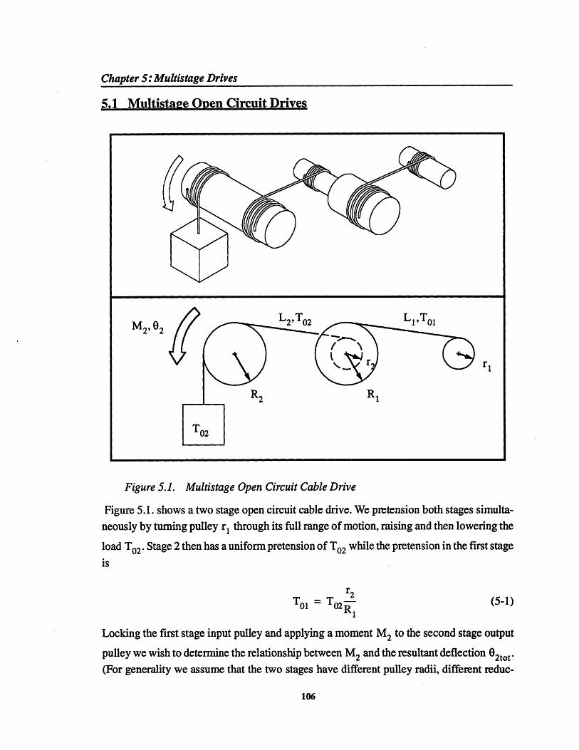
Signature of Author___ -..Department of Mechanical Engineering, Massachusetts Institute of Technology/Woods Hole Oceanographic Institution
Certified b+ -...-.. __-__ .- ---..-- --Dr. Dana R. Yoerger, Woods Hole Oedaographic Institution, Thesis Supervisor
Accepted byDr. Arthur B. BaggeroerChairman, Joint Committee fofKpied len and Engineering,Massachusetts Institute of Teclnolo Hole eanographic InstitutionONETlC4 IT
I~ K'9~1 3nd ES.LITt1--
2
The Load/Deflection Behavior of Cable/Pulley
Transmission Mechanisms
by
Edward Ramsey Snow
Submitted to theMassachusetts Institute of Technology/
Woods Hole Program in Oceanography and Oceanographic Engineeringin partial fulfillment of the requirements of the Degree of
Master of Science
Abstract
Mechanical transmission mechanisms enable a designer to match the abilities (e.g. velocity,torque capacity) of an actuator to the needs of an application. Unfortunately the mechanicallimitations of the transmission (e.g. stiffness, backlash, friction, etc.) often become thesource of new problems. Therefore identifying the best transmission option for a particularapplication requires the designer to be familiar with the inherent characteristics of each typeof transmission mechanism.
In this thesis we model load/deflection behavior of one particular transmission option;closed circuit cable/pulley transmissions. Cable drives are well suited to force and positioncontrol applications because of their unique combination of zero backlash motion, highstiffness and low friction. We begin the modelling process by determining the equilibriumelongation of a cable wrapped around a nonrotating pulley during loading and unloading.These results enable us to model the load/deflection behavior of the open circuit cabledrive. Using the open circuit results we model the more useful closed circuit cable drive.We present experimental results which confirm the validity of both cable drive models andthen extend these models to multistage drives. We end by discussing the use of thesemodels in the design of force and position control mechanisms and comment on the limi-tations of these models.
Thesis Supervisor: Dana R. Yoerger
3
4
Table of Contents
1 Introduction
1.1 Transmissions1.2 Problem Statement1.3 Why Study Cable/Pulley Transmissions?1.4 Introduction To Cable/Pulley Transmissions
1.4.1 Open Circuit Cable Transmissions1.4.2 Closed Circuit Cable/Pulley Transmissions
1.5 Summary of Results1.6 Thesis Overview
Mechanics of Wrapped Cable2.1 Wrapped Cable on a Non-rotating Pulley2.2 Modelling
2.2.1 The Slip Condition2.2.2 The Affected Angle of Wrap2.2.3 Tension Profile in a Wrapped Cable2.2.4 Elongation During Loading2.2.5 Elongation During Unloading2.2.6 Energy Dissipated During Loading2.2.7 Energy Stored During Loading
2.3 Consistency Checks2.3.1 Conservation of Energy2.3.2 Efficiency Limit of Tension Element Drives
2.4 Conclusions
3 Open Circuit Cable/Pulley Drives3.1 The Open Circuit Cable Drive3.2 Modelling
3.2.1 The Geometry-Friction Number3.2.2 Deflection During Loading3.2.3 Deflection During Unloading3.2.4 Comments on the Validity of Open
3.3 Experimental Confirmation3.3.1 Approach3.3.2 A Typical Trial3.3.3 Correlation Coefficients: All Trials3.3.4 Coefficient of Friction: All Trials
4.2.1 Equilibrium Equations During Loading 774.2.2 Equilibrium Equations During Unloading 784.2.3 Special Case I: Widely Separated Pulleys 804.2.4 Special Case II: Narrowly Separated Pulleys 834.2.5 General Case Solutions 884.2.6 Approximate Solutions for the General Case 93
4.3 Experimental Confirmation 974.3.1 Approach 974.3.2 A Typical Trial 994.3.3 Correlation Coefficients: All Trials 1004.3.4 Coefficient of Friction: All Trials 101
5.2.1 Two Antagonistic Multistage Open Circuit Drives in Parallel 1115.2.2 Individual Closed Circuit Drives in Series 112
5.3 Conclusions 115
6 Designing Cable Drives 1176.1 Suitable Applications 1186.2 Choosing the Appropriate Model for a Given Cable Drive 1206.3 Performance Characteristics and Design Parameters 121
2 The Mechanics of Wrapped Cable 172.1 Linearly Elastic Cable Wrapped Around a Non-rotating Pulley 182.2 Schematic of Approach 192.3 Free Body Diagram of Wrapped Cable Segment 202.4 Wrapped Cable Under Load 242.5 Tensile Profile During Loading 272.6 Schematic of Wrapped Cable During Loading 282.7 Elongation of Wrapped Cable on a Non-rotating Pulley 312.8 Stiffness of Wrapped Cable on a Non-rotating Pulley 322.9 Schematic of Wrapped Cable During Unloading 342.10 Tensile Profile During Unloading 372.11 Continuously Driven Pulley Under Load 432.12 Affected Angles of Wrap and Tensile Profiles 45
3 Open Circuit Cable/Pulley Drives 513.1 Single Stage Pretensioned Open Circuit Drive 523.2 Deflection of an Open Circuit Drive During Loading 573.3 Stiffness of an Open Circuit Drive During Loading 583.4 Deflection of an Open Circuit Cable Drive During Unloading, GF=0 603.5 Wrap Deflection and Dimensionless Moment vs. Time, Trial 145 663.6 Dimensionless moment vs. Normalized Deflection, Trial 145 673.7 tl and t u vs. §wr, Trial 145 683.8 Correlation Coefficients, Trials 36 through 188 69
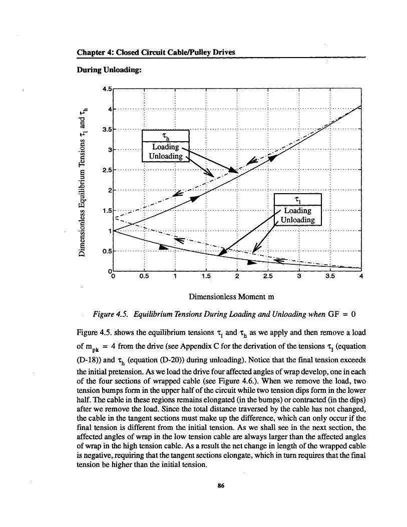
4 Closed Circuit Cable/Pulley Drives 734.1 Closed Circuit Cable Drive. 744.2 Closed Circuit Drive with Widely Separated Pulleys 804.3 Closed Circuit Drive with Narrowly Separated Pulleys 834.4 Fixed Load Stiffness vs. Initial Pretension 854.5 Equilibrium Tensions During Loading and Unloading when 864.6 Affected Angles of Wrap and Tension Bump Locations 874.7 Equilibrium Deflections During Loading and Unloading When 884.8 Dimensionless Tension vs. Dimensionless Moment, Various Values of 89
9
4.9 Dimensionless Tension vs. Dimensionless Moment, Various Values of 904.10 Normalized Affected Angles of Wrap vs. Dimensionless Moment 914.11 Dimensionless Moment vs.Normalized Deflection 924.12 Dimensionless Moment vs.Normalized Deflection. 934.13 Accuracy Approximate Model I without Wrapped Cable Term 944.14 Accuracy of Approximate Solution I with Wrapped Cable Term 954.15 Accuracy of Approximate Solution II 964.16 Dimensionless moment vs. Normalized Deflection, Trial 19 994.17 l and tu vs. wr, Trial 19 1004.18 Correlation Coefficients, Trials 1 through 30 101
5 Multistage Drives 1055.1 Multistage Open Circuit Cable Drive 1065.2 Multistage Closed Circuit Drive Made from Two Multistage Open Circuit 111
Drives5.3 Multistage Closed Circuit Drive Made from Cascaded Single Stage Closed 112
Circuit Drives
6 Designing Cable Drives 1176.1 Crossed and Uncrossed Methods of Rigging Cable Drives 125
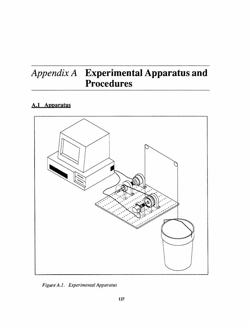
A Experimental Apparatus and Procedures 127A.1 Experimental Apparatus 127A.2 Detail of Experimental Apparatus 128
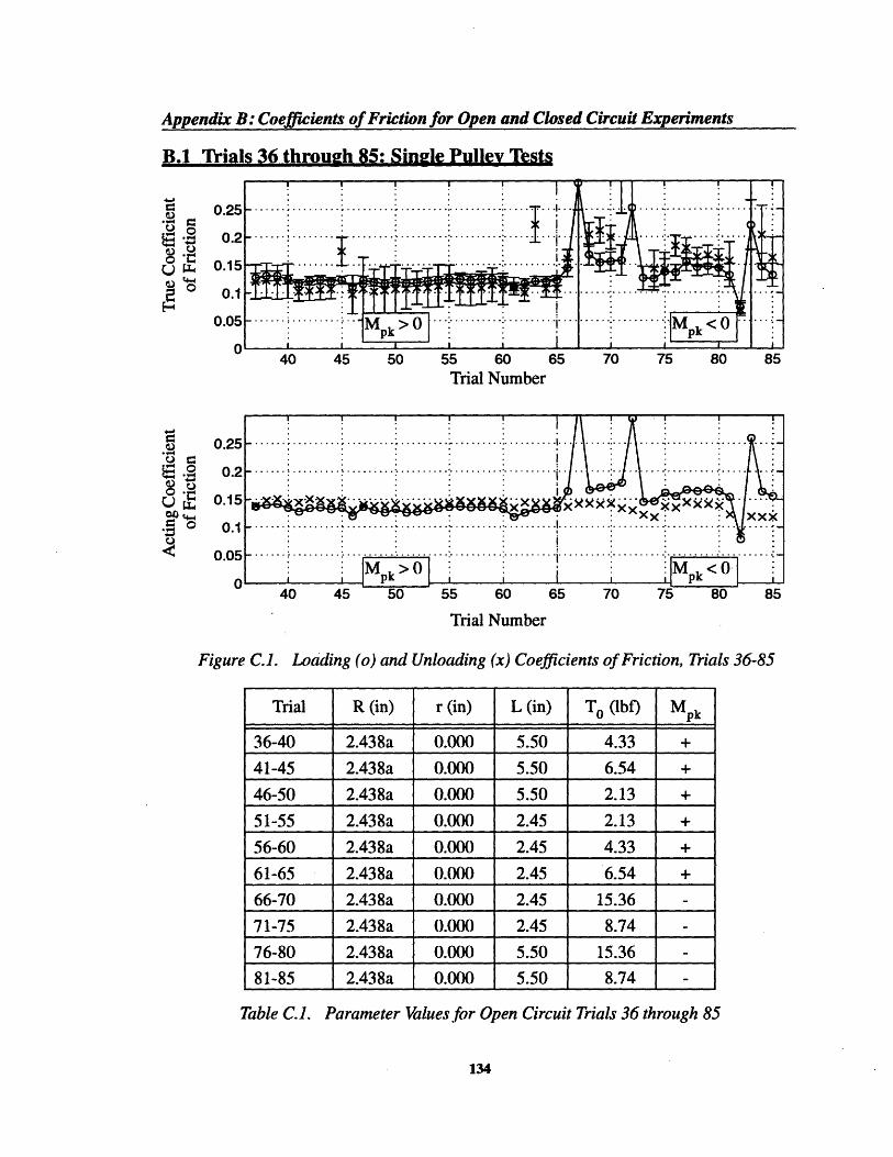
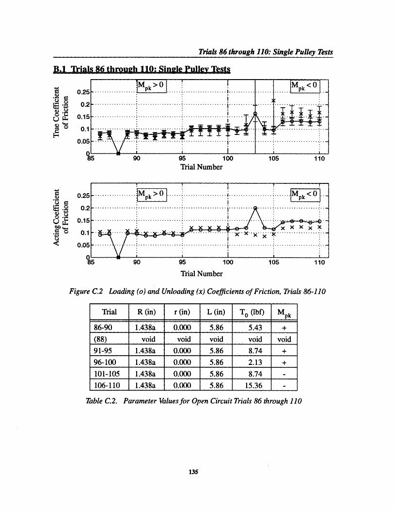
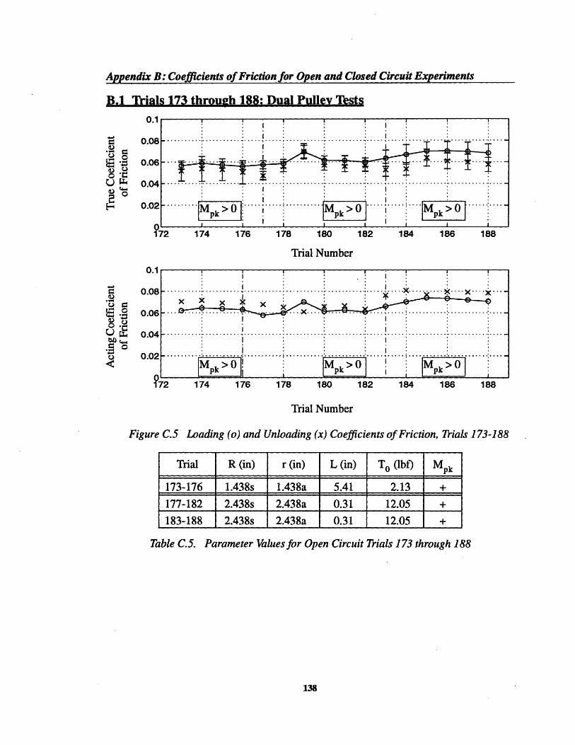
B Coefficients of Friction for Open and Closed Circuit Experiments 133B.1 Loading (o) and Unloading (x) Coefficients of Friction, Trials 36-85 134B.2 Loading (o) and Unloading (x) Coefficients of Friction, Trials 86-110 135B.3 Loading (o) and Unloading (x) Coefficients of Friction, Trials 111-135 136B.4 Loading (o) and Unloading (x) Coefficients of Friction, Trials 136-172 137B.5 Loading (o) and Unloading (x) Coefficients of Friction, Trials 173-188 138B.6 Loading (o) and Unloading (x) Coefficients of Friction, Trials 1-30 139
C Special Case II: Exact Tensions During Unloading 141
10
Chapter 1 Introduction
1.1 Transmissions
Ideally transmissions would be unnecessary; actuators would be compact, efficient andpowerful enough to be attached directly to the objects they control (an option known asdirect drive). Unfortunately the limitations of existing actuators make this option infeasiblefor a wide range of applications. To make up for this we use transmissions to modify theapparent characteristics ofan actuator By combining an actuator with a properly designedtransmission we create a new system whose abilities more closely match the characteristicsof our ideal actuator. These characteristics can be divided into three categories.
Output:Examples: Torque, velocity, shaft friction, etc.Many actuators (electric motors, internal combustion engines) deliver power mostefficiently at high velocity and low torque while many applications (robotics,earthmoving) require the application of high torques at low velocity. Using a trans-mission to boost the torque and reduce the velocity of the actuator we create anactuator/transmission assembly which resembles an actuator having the desiredtorque/velocity characteristics.
Packaging:Examples: Physical volume, weightAn actuator, even if it has the desired output characteristics, may still be too heavyor cumbersome to be connected directly to a given load. Using a transmissionallows the actuator to be separated from the load and placed where there is suffi-cient room or weight bearing capability, reducing the packaging demands at theload.
Cost:We often find it cheaper to use a transmission to adapt a non-ideal actuator to aspecific application than to procure an inherently capable actuator (assuming thata capable actuator even exists). In addition, it is typically cheaper to use one ormore transmissions to deliver power from a single actuator to multiple loads thanit is to assign a separate actuator to each load (assuming that the motions of the
11
Chapter 1: Introduction
different loads are not independent).
Transmissions are not perfect, however. Each type of transmission (e.g. gears, belts, cables,chains, etc.) has its own particular physical limitations (e.g. backlash, friction, loadcapacity, etc.) which impact the new system's performance. As designers of transmissionswe must select a transmission concept whose general characteristics suit our applicationand then tailor the specific characteristics of an implementable version to the task require-ments.
1.2 Problem Statement
We seek in this report to identify and model the physical characteristics of closedcircuit cable/pulley transmissions to assist the transmission designer in the evalu-ation, design, and optimization of cable/pulley transmissions.
1.3 Why Study Cable/Pulley Transmissions?
Cable/pulley transmissions combine zero backlash motion and high stiffness with uniquelylow stiction/friction levels, a very desirable combination in force/torque control applica-tions. Backlash severely impacts closed loop bandwidth (Schempf [11]) whereas stictioncan limit the force resolution of a system by inducing limit cycling (Townsend and Salis-bury [15]). High stiffness, of course, helps increase system bandwidth. As a consequenceof these features we find cable drives used most frequently in two applications requiringhigh performance force/torque control; robotics (Schempf [11], Townsend [15], Salis-bury[9], Dipietro [3]) and telerobotics (Goertz[5], Vertut[16], Bejczy [1], McAffee et.al.[7])
To remove backlash from a transmission we typically preload the mechanism by adjustingthe geometry of the mechanism until the drive elements have a slight interference fit. Thisremoves the backlash but tends to increase frictional forces due to increased internal loads.Comparing five such zero backlash transmission mechanisms (a cable drive, a harmonicdrive, a Kamo ball reducer, and cycloidal-type reducers manufactured by Dojen, Sumitomoand Redex) Schempf [11 ] found that the cable drive incurred the lowest friction penalty forremoving backlash.
In robotic and telerobotic applications small collisions and impacts which occur duringassembly and grasping tasks result in step changes in transmission loads, typically fromnear zero working load to some low amplitude peak load. To accurately transmit or respondto these changes the transmission must have a high force/torque bandwidth at low loads.Schempf [11] found that all of the above transmissions except the cable drive exhibitedstiffening spring behavior, showing minimum stiffness (and therefore minimum band-
12
Introduction To Cable/Pulley Transmissions
width) near zero working load. In contrast (as we will show) the cable drive exhibitssoftening spring behavior, having its maximum stiffness (and therefore maximum band-width) at zero working load. Therefore, qualitatively speaking, the cable drive is bettersuited to these applications.
1.4 Introduction To Cable/Pullev Transmissions
There are two different types of cable/pulley transmissions; open circuit and closed circuitdrives. To familiarize the reader we briefly describe each below.
1.4.1 Open Circuit Cable Transmissions
Figure 1.1. Open Circuit Cable/Pulley Transmission
Figure 1.1. shows a simple cable drive consisting of two pulleys linked by a single piece ofcable. This is an open circuit cable drive, defined as a drive whose cable(s) are slack unlessopposing torques are applied to the input and output pulleys. For the drive to function inboth directions we must preload or pretension the drive such that the cable never goesslack, for example, by hanging opposing counterweights from each pulley or usingopposing actuators at each pulley. Our interest in the open circuit drive stems less from itslimited practical applications than from the considerable insight its closed form modelsgive us into the behavior of the more useful (but more complex) closed circuit drive.
In this drive two pieces of cable antagonistically link the input and output pulleys. Wedefine a closed circuit cable transmission as a drive whose cables and pulleys form a closedforce path that is under tension even when no torques act upon the input and output pulleys.By definition a closed circuit drive must be pretensioned. For the drive shown, we tensionthe two cables by turning the two halves of the large pulley with respect to each other andthen clamping the pulley halves together to lock the circuit in a state of tension. Oncepretensioned, this transmission allows the input to actively drive the output in both direc-tions with no backlash.
1.5 Summary of Results
Existing Cable Drive ModelThe cable drive models presented in this report are presented as an improvement over thefirst order model commonly in use today (this model neglects the elongation of the wrappedcable in the drive). The predicted drive characteristics associated with this model are aconstant, linear stiffness, no hysteresis deflection and a minimum required pretension (i.e.the pretension required to prevent either cable from going slack during operation) of
mmaxT= where Max is the maximum applied load and R is the radius of the outputp2R ypulley.
14
Thesis Overview
New Cable Drive ModelThe new models predict substantially different behavior which we briefly summarize here.These characteristics have been verified directly or indirectly by the deflection experimentspresented in Chapters 3 and 4.
Softening spring behavior: Cable drives have very high stiffness at low loads and mark-edly reduced stiffness levels at higher loads which drop off rapidly as the applied loadincreases. In addition, the stiffness also depends on the load history of the drive.
The Geometry-Friction number: This dimensionless parameter determines the nature ofa cable drive's response to load (i.e. how nonlinear the behavior is). We encounter thisnumber in the analysis of every drive investigated in this report and it is the key to model-ling a given drive correctly.most important piece of information needed to
Hysteresis deflection: Hysteresis deflection is inherent to all cable drives. Surprisingly itis accurately predictable.
Dependence on pretension: The stiffness of an existing cable drive can be increasedsimply by increasing the initial pretension. This also reduces the hysteresis deflectionremaining after an applied load has been removed.
Minimum pretension: Depending on the drive's configuration the minimum pretensionrequired to prevent either cable from going slack during operation can be as low as
max
To = 4R' one half that predicted by the existing model.
Maximum cable tensions: The maximum cable tensions under load can be as much as30% higher than those obtained from existing cable drive models.
1.6 Thesis Overview
Chapter 1: Introduction: We describe the context of this work and discussother relevant work. We present the problem statement and outline the remainderof the report.
Chapter 2: Mechanics of Wrapped Cable: We model the behavior ofcable wrapped around a nonrotating pulley and show these results to be consistentprevious results.
Chapter 3: Open Circuit Cable/Pulley Drives: We use the wrappedcable results from Chapter 2 to model and explain the load/deflection behavior ofsingle stage open circuit drives. These are closed form models, allowing us to
15
. . Or t And .
Chapter 1: Introduction
investigate the dependence of the stiffness on particular design parameters. Weintroduce the Geometry-Friction number GF, a dimensionless parameter whichdetermines the character of a drive's response to load. We present experimentalresults confirming these models.
Chapter 4: Closed Circuit Cable/Pulley Drives: We model single stageclosed circuit drives as two antagonistically combined open circuit drives and findthat the Geometry-Friction number also determines the character of a closed circuitdrive's response to load. In general we must solve numerically, but we investigatetwo limiting cases for which there are analytical solutions and show that oneapplies to the bulk of practical drives. We confirm this approximate model experi-mentally.
Chapter 5: Multistage Drives: We show that a multistage open circuit drivebehaves exactly like an equivalent single stage open circuit drive whose GFnumber is a function of the properties of the individual stages. We identify twotypes of multistage closed circuit drives; one can be modeled as an equivalent
single stage closed circuit drive, the other must be modeled as n single stage closedcircuit drives in series.
Chapter 6: Designing Cable Drives: We start by identifying cable drivesas excellent transmissions for high performance position and force control appli-cations. We reiterate the importance of the Geometry-Friction number andsummarize its usefulness in the determining the appropriate model to use for aparticular drive. After discussing the impact of the design parameters on the drive'sperformance characteristics we end by summarizing the limitations of thesemodels.
16
Chapter 2 The Mechanics of WrappedCable
To model a closed circuit cable drive we must be able to model the cable wrapped on itspulleys. In this chapter we model the load/deflection behavior of a cable wrapped around anon-rotating pulley. We show that changing the load applied to the cable's free end affectsonly a portion of the wrapped cable and that the cable tension in this region varies expo-nentially with position. By integrating the strain associated with this profile we obtain theelongation resulting from the change in applied load. We further demonstrate that the cabledoes not return to its original length when we return the applied load to its initial value.
To check these results we verify that energy is conserved during elongation (i.e. that thework done by the applied load equals the work required to stretch the cable). As an addi-tional check we use the models to derive the efficiency limit for cable/flat belt drives,showing that the result agrees with the findings of others.
17
Chapter 2: The Mechanics of Wrapped Cable
2.1 WranDed Cable on a Non-rotating Pulley
Figure 2.1. Linearly Elastic Cable Wrapped Around a Non-rotating Pulley
To develop a model for the load/deflection behavior of wrapped cable we analyze thesystem shown in Figure 2.1. Attaching one end of the cable to the pulley we wrap the restsuch that the cable is uniformly pretensioned, i.e. such that the tension is everywhere equalto some value To0 . At some later time we change the load applied to the cable's free end
from To to Tapp, allow the system to reach equilibrium and then return the applied load to
its original value To. We wish to determine the changes in the length of the wrapped cable
resulting from these changes in applied load.
Approach:
The change in cable length (i.e. the elongation) is the integral of the change in cable strain.Determining the strain requires that we find the equilibrium tensile profile, which in turndepends on the amount of the wrapped cable affected by a change in applied load. To affectits neighbor a segment of wrapped cable must slip, i.e. the net load applied to it must exceedthe frictional force acting upon it. Therefore we must start by determining the load condi-tions under which an arbitrary segment of wrapped cable will slip before we can find theaffected angle of wrap. We summarize these dependencies in figure Figure 2.2. To find theelongation we simply start at the bottom of the list and work back towards the top.
18
Wrapped Cable on a Non-rotating Pulley:
Definingthe problem
Tensile Profile7 -TSolving the
problem
Figure 2.2. Schematic of Approach
Chapter Overview:
We attack each of these steps in a different subsection of this chapter. In the last twosections we check our results for consistency with the results of others.
2.2 Modelling2.2.1 Slip Condition2.2.2 Affected Angle of Wrap
2.2.3 Tensile Profile
2.2.4 Elongation During Loading2.2.5 Elongation During Unloading2.2.6 Energy Dissipated During Loading2.2.7 Energy Stored During Loading
2.3 Consistency Checks2.3.1 Conservation of Energy
2.3.2 Efficiency Limit of Tension Element Drives
19
Elongation
Affected Angleof Wrap
* A
---
F QI:_CHL! · -lllll lll
i
-IlY··I·V·
Chapter 2: The Mechanics of Wrapped Cable
2.2 Modelling
2.2.1 The Slip Condition
Friction between the cable and the pulley enables the cable in Figure 2.3. to remain in equi-
librium even if tensions T1 and T2 are not equal. We wish to determine how unequal these
loads must be for the cable to slip freely with respect to the pulley. In the next section weuse this result, first derived by Euler [4], to determine the portion of wrapped cable inFigure 2.1. affected by a change in applied load.
_
T
2
T
xo
Figure 2.3. Free Body Diagram of Wrapped Cable Segment
We begin by looking at the equilibrium conditions for the differential element of cable AOshown in the lower half of Figure 2.3. Summing the forces and moments acting on theelement we find that the cable will be in equilibrium (i.e. will not slip) if
ZF = = (T+AT) cos( )-Tcos( 2 )Ff (2-1)
20
Modelling: The Slip Condition
IFy = 0 = N-(T+AT)sin 2 -Tsin 2 (2-2)
:Mo = 0 = FfrR + TR- (T + AT)R (2-3)
where the coordinates x and y are aligned with the tangential and normal directions for the
element. Note that we have assumed that d << R (where d is the cable diameter) and that thestress in the cable is uniaxial and does not vary significantly over a cross section of the cable
(which should be valid if d R is valid).
As we shrink the size of the element from AO to dO, the change in tension AT across the
element becomes dT. Since dO is very small cos 2 ) 1 and sin (I) . Making
these substitutions the equilibrium constraints become
IFX = dT-Ffr = 0 (2-4)
dOIFy = N- (2T-dT) 2 = (2-5)
Mo = [Ffr -dT] R = 0 (2-6)
Recognizing the equivalence of the Y.Fx and £M O equations and dropping the second
dTd0order term -Td from equation (2-5) the equilibrium equations for the differential
2element of cable become
Ffr = dT (2-7)
N = TdO (2-8)
Assuming the Coulomb model of friction applies we can say that
_Ffrl < gN = TdO (2-9)
where g is the coefficient of friction between the cable and pulley. Using equation (2-7) to
eliminate Ffr from (2-9) we get
IdTj < TdO (2-10)
21
Chapter 2: The Mechanics of Wrapped Cable
gTdO is the maximum supportable tension difference (i.e. net force) that the element canresist without slipping. In general a differential element of cable will not slip as long as
IdTI = dT <T (2-11)dO dO
We call equation (2-11) the differential slip condition. It states that a differential element of
cable will not slip until the magnitude of the slope of its tension dT exceeds the product ofdo
the local tension T and the coefficient of friction . Conversely, an element of cable will
dTcontinue to slip until the magnitude of the tensile slope equals tT.
To find the load capacity of the entire arc of cable we sum the individual load capacities ofevery element in the cable by integrating the differential slip condition. Rearranging terms
and recognizing that the tension T is always positive we can write
IdTI = dT adO (2-12)T T
Integrating from one end of the angle of wrap to the other we get
T2 ow
IdT < I dO (2-13)
T. O
This leads to two different solutions, the result depending on the sign of dT.
If T2 > T dT is positive and we get
log 2 < IOw (2-14)
T 2< 5e ~ ° (2-15)
dT is negative and we get 1
If T2 < T1 dT is negative and we get
22
Modelling: The Slip Condition
T2 < e (2-16)
T 1
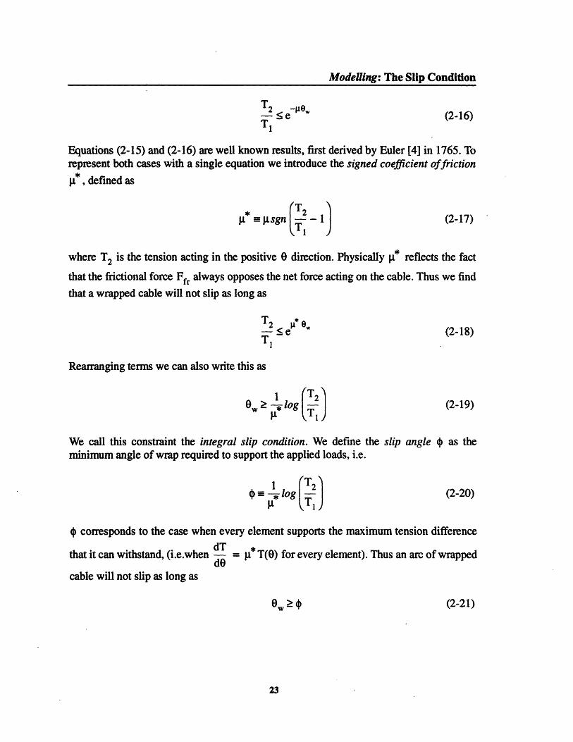
Equations (2-15) and (2-16) are well known results, first derived by Euler [4] in 1765. Torepresent both cases with a single equation we introduce the signed coefficient offriction
g , defined as
g -I sgn T. 1 (2-17)
where T2 is the tension acting in the positive 0 direction. Physically g* reflects the fact
that the frictional force Ffr always opposes the net force acting on the cable. Thus we find
that a wrapped cable will not slip as long as
T2 ow(2*-- _e (2-18)T
Rearranging terms we can also write this as
0w 1 log T. (2-19)
We call this constraint the integral slip condition. We define the slip angle 4 as theminimum angle of wrap required to support the applied loads, i.e.
*4log jT (2-20)
* corresponds to the case when every element supports the maximum tension difference
that it can withstand, (i.e.when dT = p. T(O) for every element). Thus an arc of wrappeddO
cable will not slip as long as
Ow>d (2-21)
23
Chapter 2: The Mechanics of Wrapped Cable
2.2.2 The Affected Angle of Wrap
Figure 2.4. Wrapped Cable Under Load
Returning to the system shown in Figure 2.1. we wish to find the affected angle of wrap0 aff, defined as the region of cable whose tension changes from its initial value To when
we change the load applied to the cable's free end from To to Tapp.
We begin by considering a differential element of cable dO located at the cable's point ofdeparture. The differential slip condition (2-11) states that the element will not slip if
dT < r (2-22)
At the instant we change the load the tensions acting on either side of the element dO differdT
by the finite amount Tapp - To which means that the slope dO = +o0 Thus the element
must slip and (since any change in applied load, however small, results in an infinite slope)and it starts to do so the as soon as the applied load begins to change. During slip the changein tension across the element equals the frictional force acting on the element or
dT = Ffr = ld appdO (2-23)
where the gd* is the signed version of the dynamic coefficient of friction. Consequently
the tensions acting on the adjacent element now differ by the amount (Tapp - Ffr) - TO
and, by the same argument presented above, this element must also slip. The affected region
24
[T^ (t<O) ]
VŽ (t; )
0
Modelling: The Affected Angle of Wrap
continues to grow in this way until the sum of the frictional forces acting on the affected
elements exactly equals the change in applied load, i.e. until Oaff reaches equilibrium. In
the previous section we showed that to be in equilibrium an arc of cable must satisfy the
aggregate slip condition (2-19). Applying that result we see that 0 aff stops growing when
1 Tapp0 aff = ) = log app (2-24)
P d T0
where
*= d dSg Tapp 1) (2-25)
(Cotterill [2], in his 1892 study of flat belt power transmissions, appears to have been the
first to recognize that Oaff = )). Obviously equation (2-24) only applies if Ow > . If
Ow < ) the affected angle of wrap is clearly
Oaff = w (2-26)
For all the systems analyzed in this report we assume that Ow > ), i.e. that equation (2-24)
applies. There are several important implications of equations (2-24) and (2-26);
1. Wrapped cable exhibits no stick/slip behavior during loading
2. Wrapped cable's equilibrium behavior depends on the
dynamic coefficient offriction 9d
3. If Ow > ) changes in applied load do not affect the tension
at the cable termination point (i.e. the tension at the termi-
nation is always To).
4. If 0w > ) the response of wrapped cable to applied loads isindependent of the angle of wrap 0w.
It may seem odd that the results depend on d* instead of the static coefficient of friction
gs ·To understand this we consider the last element to be affected before 0 aff reaches equi-
librium (i.e. the element at 0 = 0). Once its tension changes the element responds byincreasing or decreasing in length. As this happens every other element in the affectedregion must also slip by this amount, meaning that every element in the entire affectedregion is slipping just prior to reaching equilibrium. During slip the dynamic coefficient of
25
Chapter 2: The Mechanics of Wrapped Cable
friction Id* determines the frictional force acting on the elements. These forces act on the
elements until the region reaches its final elongation, at which point the tensile profile asso-
ciated with gd* is locked in place by the higher static coefficient of friction As*. By
applying the same arguments one can show that Id* also determines the response to any
further changes in the applied load. Thus the behavior of a wrapped cable at static equilib-
rium is determined by the dynamic coefficient of friction ld* . (These results tell us that we
should use gId* in the integral slip condition (2-19)). Unless otherwise noted the use of It
in this report refers to the dynamic coefficient of friction Itd.
2.23 Tension Profile in a Wrapped Cable
We shall now determine the equilibrium tensile profile T(O) in the affected region after
changing the applied load from To to Tapp'
While determining the affected angle of wrap we showed that the equilibrium tensiondifference across a differential element of cable in the affected region is
dT = I*TdO (2-27)
where i = d as given by equation (2-25). To solve for the tension T(O) at position 0
we rearrange terms and integrate from 0 = 0 to 0 = 0 to get
T(O) 0
J dT = *dO (2-28)TTo 0
log T () * 0 (2-29)
T(0) = Toef 0 (2-30)
where 0 < 0 < aff = 4 and we measure 0 from the interior edge of the affected angle of
wrap as shown in Figure 2.4.
Recalling that g* = sgn -p I we see that the tension profile varies exponentiallyTo
26
Modelling: Elongation During Loading
from 0 = 0 to 0 = , decaying when Tapp < To and increasing when Tapp > To (we show
the latter case in Figure 2.5.) Euler[4] was the first to show that equation (2-30) applies tothe cable in Figure 2.3. just prior to slip. We believe Cotterill [2] was the first to recognizethat it applies to a belt (or cable) at static equilibrium on a stationary pulley
Figure 2.5. Tensile Profile During Loading
2.2.4 Elongation During Loading
Referring to Figure 2.6., we wish to determine how changing the applied load from To to
Tapp affects the elongation of the wrapped portion of the cable. To find 8 we sum the
change in elongation of the all the differential elements in the cable. For an element defined
by an angle AO this change AS is
A = (eq - o) R AO (2-31)
where ,eq is the total strain in the element at equilibrium, eo is the initial strain associated
with the pretension To and RAO is the unstressed length of the element As we shrink the
size of the element from AO to dO, the change in the element's length A8 across theelement approaches dB and (2-31) becomes
d = (eq - o) RdO (2-32)
27
Tapp
0
Chapter 2: The Mechanics of Wrapped Cable
Figure 2.6. Schematic of Wrapped Cable During Loading
Integrating eq over the affected region gives us the total elongation of the loaded cable at
equilibrium. If the cable material obeys Hooke's law (i.e. is linearly elastic) and we assumethe cable load is uniaxial we can rewrite (2-31) as
dB= eqRdO (2-33)E
where aeq is the stress associated with the strain £eq If we also assume that the stress is
constant in the cable's cross equation (2-33) becomes
d = - ( ) RdO (2-34)EA
where T(O) is the tension in the element and A is the cross sectional area of the cable,which we assume to be constant. In section 2.2.3 we showed that the equilibrium tensionvaries exponentially from To to Tapp across the affected angle of wrap. We consider now
an arc of cable P within this region for which the tensions acting on the left and right handends are T1 and T2 respectively. The tension profile in the region 0 < ' < is
T(O') = T e = (2-35)
where 0' is measured from the left end of 13 and
28
}
6
- -
Modelling: Elongation During Loading
* = gsgn T - 1 = sgn TT I) (2-36)
Using equations (2-34) and (2-35) and integrating we can write the elongation as
f RT 1 P 0,J dB = EA e dO' (2-37)
0 0
RT1·aeq3 EA* (e -1) (2-38)
Req3 = EAR* (T 2 -T 1 ) (2-39)
where we have recognized that Ti e p = T(1B) = T2. Thus we see that the total elonga-tion (relative to the unstressed length) of an exponentially loaded cable is proportional to
the difference between the tensions applied to its ends. (Note that g ensures that 8 eqp is
always positive regardless of the relative size of T1 and T2 ).
To find the initial elongation 60p of the cable in P we return to equation (2-31) and integrate
the Eo term across to get
To RI d8o = I EA dO' (2-40)
o o
ToR8 = -T 0R (2-41)
3 - EA
Thus we find the net change in elongation of the cable in P by subtracting the initial elon-gation 860 from the equilibrium elongation 8 eq13 to get
8 = 8 eq - 8O, (2-42)
29
Chapter 2: The Mechanics of Wrapped Cable
R6= EA* (T2 -T -To* ) (2-43)EAR T 2 -- 0 3)
Equation (2-43) applies to any exponentially loaded arc of cable P whose initial tension
was uniformly equal to To.
To apply this result to the entire affected angle of wrap we substitute To , Tapp and 0 aff for
T1, T2 and i to get
8= R * (Tapp-To ea) (2-44)EA* app - T - af
If O > we can substitute 0 aff = 4 which yields
RT r T app Tapp|= -1 E-l (T 0 ) (2-45)
EA T 0T
Equation (2-48) gives deflection of a uniformly pretensioned cable when we change theload applied to its free end from To to T app' The earliest appearance of this result appears
to be that presented by Green [6] in his 1955 publication on continuous flat belt drives.
To find the associated stiffness k we differentiate (2-48) with respect to T app and rearrange
terms to get
dTapp - EA* Tapp dB R Tapp-T) (2-46)
We find it convenient to introduce the dimensionless tension x, defined as
TappToapp (2-47)
T
Making this substitution equations (2-48) and (2-46) become
RT08 = * ( --1-logT) (2-48)EAand
and
30
Modelling: Elongation During Loading
E * R
k EAt* (T) (2-49)
while Oaff and * become
10 aff = logtg.
(2-50)
g* = sgn (- 1). (2-51)
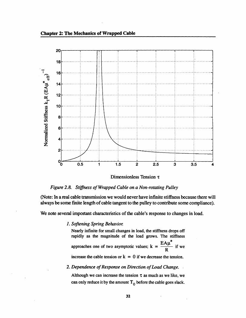
Figure 2.7. and Figure 2.8. show plots of the normalized elongation and normalized stiff-
ness of the wrapped cable as a function of t (recall that 9l* changes sign at = 1 i.e. when
Tapp = T)
-I'.,ma
Figu
-2 -1.5 -1 -0.5 0 0.5 1 1.5 2
Normalized Elongation 8 (EAI,*eff) (RTo)-1
ire 2.7. Elongation of Wrapped Cable on a Non-rotating Pulley
31
Chapter 2: The Mechanics of Wrapped Cable
I
C4ea4._rA
OZ
Dimensionless Tension
Figure 2.8. Stiffness of Wrapped Cable on a Non-rotating Pulley
(Note: In a real cable transmission we would never have infinite stiffness because there willalways be some finite length of cable tangent to the pulley to contribute some compliance).
We note several important characteristics of the cable's response to changes in load.
1. Softening Spring Behavior:
Nearly infinite for small changes in load, the stiffness drops offrapidly as the magnitude of the load grows. The stiffness
approaches one of two asymptotic values; k = EA* if weR
increase the cable tension or k = 0 if we decrease the tension.
2. Dependence of Response on Direction of Load Change.
Although we can increase the tension as much as we like, we
can only reduce it by the amount To before the cable goes slack.
32
Modelling: Elongation During Unloading
As the applied load approaches zero the affected angle of wrap
10 aff = -logx approaches infinity. The tension in this region
approaches zero resulting in a large deflection as this substantialamount of cable contracts. Increases in tension, however, have
much less impact on the growth of 0 aff, resulting in more
modest deflections.
3. Dependence of Stiffness on Pretension To.
By substituting Tapp = T o + AT into equation (2-46) we get
EAg* (To+AT /k = E.iR (OAT). The two asymptotic stiffnesses
mentioned above are unaffected by T o. For small AT, however,
weEget kTwe get k EA RT) and we see that the stiffness is
roughly proportional to the pretension T o.
2.2.5 Elongation During Unloading
Referring to Figure 2.9. we assume that the load Tapp applied to the cable has been changed
from the initial uniform value To to some peak value Tpk and allowed to reach equilibrium
so that
T(O) = T~e e (2-52)
and
1aff log (2-53)
where
1.*To n) _ (2-54)
At some time t we return the applied load to some intermediate value Tapp which lies
33
Chapter 2: The Mechanics of Wrapped Cable
between To and Tpk. We wish to find the equilibrium elongation 6 associated with this
loading sequence. To do so we follow the same steps used to find the elongation duringloading; identify the region of cable affected by the change in applied load, determine thenew tensile profile, and use this profile to find the change in elongation.
Figure 2.9. Schematic of Wrapped Cable During Unloading
Affected Region:
We define a new affected angle of wrap x defined as the region of cable whose tensionchanges from the equilibrium profile (2-52) when we reduce the applied load from its peakvalue. To begin we consider a differential cable element at the cable's departure point as we
begin to at the instant we change the load from the peak load Tpk to Tapp' If the element
does not slip there will be an abrupt change in tension across it so that dT = o. However,dO
applying the differential slip condition (2-11), we see that this element can only be in equi-
librium if dT| < 4T pk Therefore the element must slip and begins to do so the instant thedO
load starts to change, initiating the growth of a. This region continues to grow until it
reaches equilibrium, i.e. when a satisfies the integral slip condition (2-19). Applying (2-19) we get
1 Tapp= **log PP (2-55)
g Tb
34
To (t <0)
Tpk (O<t>t l)Tapp (t>t l )
6
1
Modelling: Elongation During Unloading
*b* R t~sgn -Ta1PP )(2-56)
We can show, however, that g* = -m*. To verify this we consider the two possibleloading scenarios. If we initially increase and subsequently decrease the applied load then
Tpk > To and Tb > Tapp which, applying equations (2-54) and (2-56), leads to * = p and
l * = -. An initial decrease and subsequent increase in applied load mean that Tpk < TO
and Tb < Tapp in which case = - and = . Thus holds and we can
rewrite equation (2-55) as
1 Tappa = -- log app (2-57)
Tb
By the definition of a the tension Tb acting on the left hand end is
Tb = T(Oaff-() - Toe (Off a) (2-58)
where 0 = aff - a is the location of the left hand side of a. By substituting into the equi-
librium condition (2-57) we find that the new affected angle of wrap continues to grow until
I Tapa = log app (2-59)
p Toe a) (2-59)
Rearranging terms we get
eT = ) (2-60)
app (e 2a (2-61)
To
Finally we use equation (2-53) to eliminate Oaff and solve for a to get
1 Tpka = 2 logT (2-62)
Tapp
35
Iws9luulm�D·r�·�··uulr�rr�·�-·l-·-----
Chapter 2: The Mechanics of Wrapped Cable
This is the portion of Oaff affected by changing the applied load from its peak value Tpk to
the Tapp,
Tensile Profile:
When the cable reaches equilibrium every element in the new affected region0 aff - a < 0 5 aff supports the maximum load that it can withstand without slipping, i.e.
dT = -g* TdO (2-63)
where the minus sign reflects, as we showed above, that the friction force now acts in the
opposite direction of the friction force associated with the original affected angle Oaff. To
find the new tensile profile we rearrange terms and integrate across the region to get
T.Pp 8 aff
IdT * dO (2-64)
T(O) 0
T(0) = Tappe (2-65)
Eliminating 0 aff the tensile profile a becomes
T TT(O) = Tapp pk e-* 0 (2-66)
To
Thus the tensile profile over the original affected region is
TeA ° [(
T(0) = TappTpke [goToe [
To find the tension Tb at the boundary between the two affected regions we substitute
0 = aff - a into either equation (2-65) or (2-66) to get
Tb = JTappTpk (2-68)
Thus Tb equals the geometric mean of the peak load Tpk and the present load Tapp
36
(2-67)
Modelling: Elongation During Unloading
Figure 2.10. Tensile Profile During Unloading
Figure 2.10. shows the tension profile when we increase (i.e. Tpk > To) and subsequently
decrease the applied load Tapp. Friction, capable of supporting a tension difference in either
direction, traps a record of the cable's load history so that the wrapped cable becomes a sortof mechanical memory device. We call the profile shown in Figure 2.10. a tension bump. Ifwe had initially reduced and then increased the tension Tapp (i.e. if Tpk < TO) the tension
at a would be lower than the surrounding tension and we would have a tension dip.
To "erase" any knowledge of the previous load Tpk we decrease Tapp until a grows to
equal aff or
1 Tpk 1 TpkloTk 2 Tp10 (2-69)
9 To 2g Tapp
Tapp ToTo Tpk (2-70)
or in dimensionless terms when
37
- -1 T -I- r T -I
I I I I I If I I I I I I I
Tapp
0
Chapter 2: The Mechanics of Wrapped Cable
SC = - (2-71)tpk
If we instead keep Tapp constant and rotate the pulley counter clockwise, the tension bump
rotates intact with the pulley while new cable wraps onto the pulley with constant tension
Tapp If we keep Tapp constant and rotate the pulley clockwise an amount , by defining
Oaff' = aff - P and substituting for 0 aff in equation (2-61) we find the new tension bump
location a' is
(' = a p (2-72)app 2
where aapp is the bump location before we rotated the pulley. To "erase" any knowledge of
the original load Tpk we must turn the pulley until Oaff' = a ' or
0aff-P = laapp 2 (2-73)
which becomes
I TappTpk[3 = 2 (aff- aapp) = Og pp pk (2-74)
T2
Elongation:To find the elongation associated with this tension bump we add the elongations associated
with each of the two regions 0 < 0 < (aff - a) and a < 0 < 0 aff. Applying equation (2-
43) to each region we find that the elongations of the two sections are
Ra EA* (Tb-Tapp- Ta) (2-75)
= EA* (Tb-To-± To (aff a)) (2-76)
Adding these we find that the elongation of the tension bump relative to the its initialuniformly pretensioned state to be
38
Modelling: Energy Dissipated During LoadingR~~~~~~~~~~ ,*
,= * (2 Tb - T - Tapp - To0aff) (2-77)
Substituting for Tb and Oaff we get
8 = R *2|-T -TTapp -T log T, (2-78)EARap To
or, in terms of the dimensionless tension r, this becomes
RTo
6 = EA-* (2 -1tP - -tlogpk) (2-79)
2.2.6 Energy Dissipated During Loading
Because of friction the stretching cable dissipates energy as it slips against the pulley.Referring to Figure 2.6. the work done by friction at a position 0 is
dW = Ffr(O)6(O) (2-80)
where Ffr(O) is the frictional force at 0 and 6(0) is the total length of cable that slides past
this point as the system approaches equilibrium. We showed in section 2.2.1 that
Ffr(O) = * T(O)dO (2-81)
By substituting the equilibrium tensile profile T(O) = Toe 0ethis becomes
Ffr(O) = Toee* d O (2-82)
To find the elongation at position 0 we apply equation (2-43) to the arc of cable subtended
by 0 to get
8(0) = * (Te - T T-T og* 0) (2-83)EAtion (2-80) we get
Eliminating Ffr(O) and 8(0) from equation (2-80) we get
39
Chapter 2: The Mechanics of Wrapped Cable
dW = (*T 0e d0d) TOR (e -1-'*0) (2-84)
By integrating over the region 0 < 0 < aff we find the total energy dissipated during elon-
gation.
Wd 2 Off
dW = ° (e 2 °-eL - *0eP O)dO (2-85)
0 0
Noting that the last term in parentheses requires integration by parts this becomes
T2 R 1 2p *0
W = 0 * -e -ee */ p*0 -e 0 )diss EAi* 2 0
(2-86)TOR Cl 2o*0 0
a
EAjx 2e -S 0
1If 0w > equation (2-24) tells us that 0 aff = * logr. Making this substitution we find that
the energy dissipated by stretching the cable is
W diss =2T -Roger 1E (2-87)
2.2.7 Energy Stored During Loading
Additional work, stored as strain energy in the elongated cable, is required to change thelength of the affected cable. The work dW done in stretching a differential element ofwrapped cable is
dW = T(O)d6(0) (2-88)
where T(O) is the equilibrium tension in the element and d(0) is the amount by which itslength changes in response to the applied load (we assume that the change in tension acrossthe element is much much smaller than the tension T(O) itself). Using equations (2-30) and(2-31) to eliminate T(O) and d6(0) we can rewrite (2-88) as
40
Consistency Checks: Conservation of Energy
dW = (T e ) d (2-89)0 EA
where we have also made the appropriate substitutions for Eeq and Eo in equation (2-31).
We find the work required to stretch the entire affected angle of cable by integrating over
the region < 0 < e0 aff.
Walored 2 rff
ToR 2| dW= - A ( e -ep )dO (2-90)
0 0
stored = EA* -e 2-
1Again, if the wrap angle 0 > equation (2-24) tells us that 0aff = -log () and we get
2Wstored EA* 2T - 't + (2-92)
or
ToRWo ( 1) 2 (2-93)stored - )2EAg
2.3 Consistency Checks
2.3.1 Conservation of Energy
If our results are correct the work done by the by the applied load during elongation shouldequal the sum of the dissipated and stored energies or
Win = Wdiss + Wstored (2-94)
The work done by the applied load is
41
Chapter 2: The Mechanics of Wrapped Cable
Win =Tapp dx = TappS (2-95)
where 8 is the equilibrium deflection at the point at which Tapp is applied and we assume
Tapp is independent of 6. Using equation (2.48) to replace 8 and rearranging terms we find
the work done by the applied load during elongation to be
RT2W RT ( 2 - logr) (2-96)
Returning to equation (2-94) we add Wdiss and Wstored to get
diss stored EAL ( )+ 2 (2-97)RTo 2 1 2 2 121
which simplifies to
RT2
w + W T _ -- log) (2-98)diss stored EA (2-98)
Comparing equations (2-96) and (2-98) we see that the models are consistent with the prin-ciple of energy conservation.
2.3.2 Efficiency Limit of Tension Element Drives
We now show that the results of the previous sections are consistent with the steady stateefficiency limit predicted by Green [6], Tordion [13], and Townsend [15]. Green andTownsend determined the power loss by comparing power in to power out. Tordion derivedthe efficiency limit by determining the frictional power loss due to slip between the belt andpulley but did so by formulating the problem as an analogous compressible fluid flowproblem. We also determine the frictional power loss but we use a more classical mechanicsbased approach employing the models we have developed.
42
Consistency Checks: Efficiency Limit of Tension Element Drives
Problem Statement:
Figure 2.11. Continuously Driven Pulley Under Load
We consider the steady state rotation of the system shown in Figure 2.11. The pulley R
rotates at a constant angular velocity Q and the working load M exactly balances themoment resulting from the difference in cable tensions, i.e. the system is in dynamic equi-librium.
As Reynolds [8] first recognized, the cable on the output pulley R must stretch as it travelsfrom the low tension side to the high tension side and therefore must slip with respect to the
pulley surface. Similarly, the cable on input pulley r must also slip, only here it must stretchas the pulley rotates. We wish to determine the continuous power dissipation associatedwith these regions of slipping cable.
The Affected Angles of Wrap and Tensile Profile
Swift [12] showed that the affected angle of wrap and the tensile profile in this system arestationary with respect to a non-rotating world frame of reference. To see this we consider
the drive initially at rest and uniformly pretensioned to T0 . Locking the position of the
input pulley r we apply the load M to the output pulley. As a result the cable tensions
43
T I MR
T
.... _ . _ _-11· 111-
Chapter 2: The Mechanics of Wrapped Cable
change to Th and T and two affected angles of wrap develop on each pulley;
1 Th o1 To0affh log -on the upper halves and -af, log - on the lower halves (see Figure
2.12.a. For clarity we have assumed that the affected regions do not overlap, i.e. that they
are still separated by an arc of cable at tension To).
Maintaining the applied load we slowly rotate the input pulley r in the clockwise direction,
thus tending to decrease 0affh and increase Oaff, on the output pulley R. However, (still
referring to the output pulley) the loads acting on the ends of 0 aff are still To and Th so
T h
by the slip condition 0 affh must still equal - log aff, on the other hand, does in fact
T oincrease. The original affected region 0 aff log rotates intact with the output pulley
aff T1
while new cable wraps on behind it at constant tension T1 (Figure 2.12.b.). Eventually this
region of constant tension extends into the interior edge of the upper affected angle, after
which only the upper affected angle of wrap 0 aff, remains, its value now equal to
Oaffh = log T J (2-99)
(Figure 2.12.c.). During constant rotation the entire arc of cable defined by 0 affh slips
dTcontinuously so the slope of the tension in this region is = lT. The tensile profile in
dO
the affected angle of wrap is therefore
T(O) = T e go (2-100)
whereas the tension in the remainder of the wrapped cable is uniformly equal to T1. Thus
T1 becomes the effective pretension for the wrapped cable. The development of the input
pulley's tensile profile is similar except that Th becomes the effective pretension and only
the lower affected region remains, equal to 0 aff = 0 aff = logaff, affh g J,
44
CO-isj~ C heckisEff cien 'l, _ .,es
' Oulles
45
Chapter 2: The Mechanics of Wrapped Cable
Power Dissipation at the Output Pulley R
Power dissipation only occurs where cable slips with respect to the pulley (i.e. in the region
0 < 0 < affh for the output pulley R). The differential power loss at a position 0 equals the
product of the frictional force and the slip velocity or
dP(O) = Ffr(O) dt (2-101)
where we recognize that the slip velocity is the time derivative of the elongation 8(0). Fromthe derivation of the slip condition in section 2.2.1 we know that
Ffr(O) = pT(O)dO (2-102)
Substituting for T(O) we get
Ffr(O) = pTe dO (2-103)
This is the frictional force at the position 0 which again is measured with respect to thestationary world frame.
Our expression for elongation of a wrapped cable gives the amount of slip at a point as a
function of 0. By the chain rule we may write the slip velocity - asdt
d8 d dod8 = d8 d0 (2-104)
dt d dt
d8To find we apply equation (2-48) to the arc of cable subtended by 0 which yields
do
8(0) = R (T eA -T -T,T0) (2-105)EAgi
and then differentiate with respect to 0 to get
d8 RT, go- RT- (eye -1) (2-106)
d = EA
Recognizing that = equation (2-104) becomesdt
46
Consistency Checks: Efficiency Limit of Tension Element Drives
d8 flRT 1 ld- = EA ( e -1) (2-107)dt EA
Substituting for d and Ffr in dP(O) we get
dP(O) = (Tle d) EA (2-108)L EA(e
To find the total power dissipation for the output pulley we integrate over the entire affectedregion to get
PLR 0'ffh 2
jI fRT 1 2.iO jO (2-109)dP(O) = (e -e )dO (2-109)
0 0
(Note that the power loss at 0 = 0 is zero since there is no slip at this point).Thus the powerloss at the output pulley PLR is
gQRT2P. - 2EA 2e + 1 T'2it (2-110)
gQRT 2 2
P LR 2EA y + 1) (2-111)TR =2EA
If we substitute aff = - log (T- and rearrange terms we get
R (T-T 2 (2-112)PLR = (Th -TI)2EA
Substituting M = (T h - TI) R we find that power loss at the output pulley R is
aMPLR = 2EA (Th -TI) (2-113)
This is the same power loss term that Townsend [15] obtained via a control volume anal-
47
.. . ._ , ,,
Chapter 2: The Mechanics of Wrapped Cable
ysis. Noting that 2M is the power delivered to the load we can rewrite equation (2-115) as
(2-114)Th- T
PLR = Put 2EA
Overall Efficiency of the Complete Drive
A similar power loss takes place at the input pulley, the only difference being that the cablecontracts as it rotates from the high tension side of the pulley to the low tension side.Performing the same analysis on the input pulley we find its power loss to be the same asthat of the output pulley, i.e.
TP - TiPL = Pin 2EA (2-115)
The power the input pulley delivers to the cables must equal the power the output pulleytakes from the cables, i.e.
ThPi -T2EATh -TI
2EA= Pout ( + (2-116)
Solving for the efficiencyPout
= we getin
Th - T1
2EAq= Th - T1 + h
2EA
Th -T 1When - < 1 (which holds for most
2EAapproximately equal to
properly designed cable mechanisms) this is
Th- -Ti M= 1- EA REA
(2-118)
which is the efficiency limit obtained by the others. Thus we conclude that our models areconsistent with previous work on the efficiency of belt and cable drives.
48
(2-117)
Conclusions
2.4 Conclusions
In this chapter we modelled the equilibrium elongation of a cable wrapped around a non-rotating pulley, first as we applied a load and then as we removed it. We summarize ourfindings below.
Characteristics of Wrapped Cable
1. Wrapped cable exhibits softening spring behavior
2. Stiffness increases as we increase pretension To.
3. Exhibits no stick/slip behavior during elongation.
4. dynamic, not .tatic, determines the equilibrium behavior5. Applied loads only affect a portion of the wrapped cable.6. Applying and removing a load creates a stable "tension
bump" in the tensile profile of the wrapped cable.
7. The elongation associated with a tension bump determinesthe hysteresis deflection of the drive.
49
Chapter 2: The Mechanics of Wrapped Cable
50
Chapter 3 Open Circuit Cable/PulleyDrives
Using the results of the previous chapter we now model the deflection of a single stage opencircuit cable drive during both loading and unloading. We show that in both cases the char-acter of the drive's response depends on the value of a dimensionless parameter we call thegeometry-friction number GE High GF values correspond to a low but relatively linearstiffness whereas low GF values represent much stiffer drives whose stiffness drops offrapidly as we increase the applied load. We also find that for low and moderate GF values
increasing the pretension To increases the stiffness. We end by presenting experimental
results which confirm the validity of both the loading and unloading models.
51
I^-I-"�--""~U~"""~~"-~IUI�"II������
Chapter 3: Open Circuit CablelPuley Drives- ~ ~ ~ ~ I I I I I
3.1 The Open Circuit Cable Drive
Figure 3.1. Single Stage Pretensioned Open Circuit Drive
Definition: An open circuit cable drive is a cable drive whose cables areonly in tension while the drive transmits a load between the input andthe output.
Figure 3.1. shows a single stage open circuit cable drive in which a length of cable couples
the rotation of the input pulley r and the output pulley R (the ends of the cable are rigidly
attached to each pulley). Prior to applying the moment M we turn the input pulley r backand forth through the full range of motion permitted by the drive cable. This ensures that
the drive is uniformly pretensioned, i.e. that the cable tension is everywhere equal to To,
the weight of the block. Locking the position of the input pulley r we wish to determine the
equilibrium deflection 0 of the output pulley R when we apply and subsequently removea moment M.
52
M,(g
Modelling
3.2 Modelling
We find the deflection of the drive by identifying and then simultaneously satisfying thesystem's geometric, constitutive and equilibrium constraints. The geometric constraint
relates pulley deflection 0 to the cable elongation, the constitutive relation relates this elon-
gation to the tension T in the cable's free length and the equilibrium constraint relates thistension to the applied moment M. In these derivations we assume that
1. the affected angles of wrap aff on the pulleys are alwayssmaller than the actual angles of wrap
2. the deflection angle 0 is much smaller than the affected angleof wrap Oaff.
Geometric Constraint:
The rotation of the output pulley is equal to the cable elongation divided by the pulleyradius R or
os;gl6 (3-1)
Equilibrium Constraint:
At equilibrium the moments acting on pulley R sum to zero, resulting in
MT = To +- (3-2)
Dividing by To we obtain the dimensionless equilibrium constraint
=l+ml (3-3)
Twhere we define the dimensionless tension z - and the dimensionless moment
Mm-.
RTo
Constitutive Relations:
The constitutive relation relates the total cable deformation 8 to the tension T in the tangent
53
Chapter 3: Open Circuit Cable/Pulley Drives
length of cable. For the open circuit drive the total cable deformation is
8 = R + L + r (3-4)
where r and R are the deformations of the cable wrapped on the pulleys r and R and 8L
is the deformation of the tangent segment of cable L. To find 8 L we simply integrate the
change in strain resulting from the change in load to get
L
fL = ( - )dx (T - T) (3-5)EA0
where E is the strain in the cable, T is the equilibrium tension in the tangent length and wehave assumed a linearly elastic cable. Note that this relation holds regardless of whether weare applying or removing a load.
The behavior of the wrapped cable, however, depends on whether we are loading orunloading the drive. Consequently we obtain a different constitutive relation for each case.
We find the constitutive relation during loading by applying equation (2-48) to find R and
sr and, making the appropriate substitutions in equation (3-4), we get
ToR ToL Tor8 =EA,* (- 1 - log) + - (-1) + * (- 1 -logs) (3-6)
EA R EA EA r
where R* = }uRsgn (T- 1) and gr = grsgn (X - 1) are the signed versions of the
coefficients of friction between the cable and each of the pulleys. When we collect termsthis becomes
TOR 1 r 1 TLEA )+(t RZ (* '--log1) (3-7). R EA
Defining the effective coefficient offriction * eff as
-1 -111 (ff = (I+ - L -- ) sgn (r - 1) (3-8)
the constitutive relation during loading (3-7) becomes
54
Modelling: The Geometry-Friction Number
TOR ToL8 = tEA* (N - 1 - log) + E- (c- 1) (3-9)
EA9.L ef EA
(Note: If the coefficients of friction for the two pulleys happen to be the same (i.e. if
Rg sen (- 1) ).Br = R = ) B* eff simplifies to * e = R +
To obtain the constitutive relation during unloading we use equation (2-79) to eliminate iR
and r from equation (3-4) which yields
ToR ToLEAPe= , (2 p I (3-10)EAB ,ff EA
By comparing equations (3-9) and (3-10) with equations (2-48) and (2-79) we see that acable wrapped around two pulleys R and r (with coefficients of friction R and r)
behaves as if it was wrapped around a single pulley R with an effective coefficient of fric-
tion of B* eff'
(Note: We have modelled all of the wrapped cable as if it were wrapped on a nonrotatingpulley. This presents no problem for cable on pulley r since we have locked it in place.Pulley R, however, rotates as the cable responds to the applied load and this may cause theaffected angle of wrap (and thereby the elongation) to differ from that predicted by thenonrotating pulley model. Nonetheless we can say that any effect will be small if the pulleyrotation 0 is very small compared to the affected angle of wrap aff expected for an equiv-
alently loaded nonrotating pulley, i.e. if 0 << ) = ,4 log (i ). In section 3.2.4 we verify
that typical open circuit drives satisfy this condition and we try to estimate the error fordrives which do not satisfy the condition.)
3.2.1 The Geometry-Friction Number
We take one last look at the constitutive relations before we solve for the drive's deflection.By combining terms we can rewrite equations (3-9) and (3-10) as
= EAi,* eff(+ Ltf )(c-1)- log(r)] (3-11)EAB eff R
55ss
Chapter 3: Open Circuit Cable/Pulley Drives
and
$ [=1EAeff (L+ R 1 (-1)-2-1ogapk (3-12)
Note the presence of the dimensionless term R- in both equation (3-11) and (3-12).R
This term indicates the relative importance of the elongations of the tangent and wrappedportions of cable. To see this we compare the elongations of the tangent and wrappedportions of cable during loading
[tan L9 eff (1 o g) (3-13)
wrap
and during unloading
tan L*eff (22 pk 2- logpk (3-14)8 R (r- 1)
LgleffWhen f >> 1 (e.g. when the pulleys are far apart) the elongation of the tangent cable
R
Leffdominates and the stiffness is very nearly linear. When - 1 (e.g. when the pulleys
Rnearly touch) the elongation of the wrapped cable dominates and the stiffness is decidedlynonlinear. Thus this parameter determines the character of a drive's response to load. Wecall this parameter as the Geometry-Friction number and designate it as
GF- L (3-15)R
L!I(In the special case of gr = lR = t this becomes GF ). In general we shall useR+r
LI* effthe signed version of GF defined as GF GFsgn (- 1) -R sgn (m) where we
R
have used the dimensionless equilibrium constraint (3-3) to replace r - 1 by m. We will
encounter the parameter GF in the analysis of every drive investigated in this report.
56
Modelling: Deflection During Loading
3.2.2 Deflection During Loading
E0E
U:co
0a,
._
C0S:
3.5
3
2.5
2
1.5
1
0.5
0
-0.5
A1-2 -1 0 1 2 3 4 5
-1Normalized Deflection (EA* effTO )
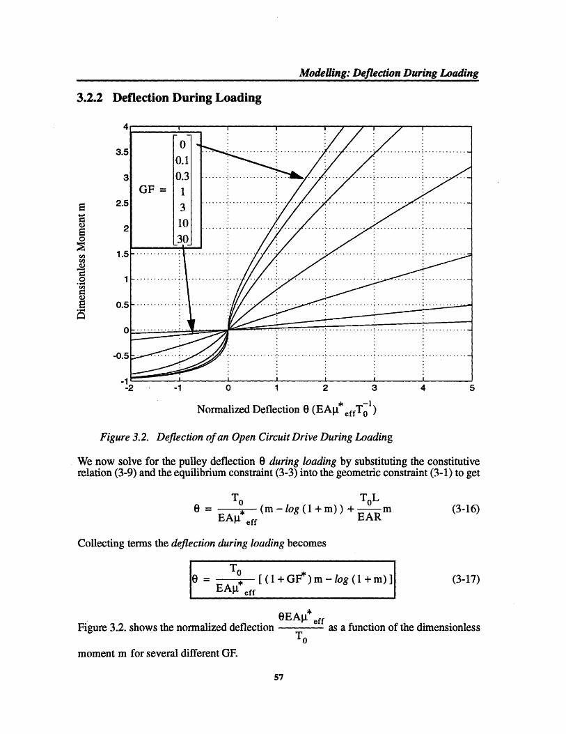
Figure 3.2. Deflection of an Open Circuit Drive During Loading
We now solve for the pulley deflection 0 during loading by substituting the constitutiverelation (3-9) and the equilibrium constraint (3-3) into the geometric constraint (3-1) to get
Collecting terms the deflection during loading becomes
0= E [( +GF*)m-log (+m)] (3-17)
0EAs* eff
Figure 3.2. shows the normalized deflection as a function of the dimensionlessmoment m for several different GF
moment m for several different GF.
57
0
0.1
GF= 1
3
30
`�"-" ""II�"U~"W~"III�-���
Chapter 3: Open Circuit Cable/Pulley Drives
The open circuit drive, like the wrapped cable examined in Chapter 2, exhibits softeningspring behavior, i.e. the stiffness decreases with increasing load. The drive's stiffness also
decreases as the value of GF increases. To better understand these trends we solve for the
drive's torsional stiffness kT by differentiating equation (3-17) with respect to M and rear-
ranging terms to get
dM dm dMkT dO de dm
EAgI* effR
m+
Eliminating GF and m and rearranging some more we get
k [(EAR + (EA* R(1 + R ))T L 9 eff
-1 -0.5 0 0.5 1 1.5 2 2.5 3 3.5 4
Dimenionless Moment m
Figure 3.3. Stiffness of an Open Circuit Drive During Loading
58
(3-18)
(3-19)
'-
0z14c
o
Modelling: Deflection During Unloadingi~ m... iii
The drive's stiffness is the series combination of the stiffness due to the tangent cable (firstterm) and the stiffness due to the wrapped cable (second term). Note that kT depends on
the pretension To, i.e the higher the pretension the higher the stiffness. This indicates that
we have some ability to change the stiffness of an existing drive without making any phys-ical modifications to it. We shall see that this also holds true for closed circuit drives.
kTFigure 3.3. shows the normalized stiffness EA4*effR as a function of the dimensionless
moment m for several values of GF. The maximum stiffness for each curve
EAieffR EAR 2
kTmax = GF L occurs at m = 0 and is equal to the stiffness due to the
tangent cable (the wrapped cable's stiffness is infinite at this point). As we apply a load thestiffness drops off rapidly, approaching zero as m - -1 (i.e. as the cable goes slack) orEAcffR
gef- flRas m + (Note that when GF > 1 changes in m have little effect on the stiff-GF+ 1
ness).
3.2.3 Deflection During Unloading
We find the pulley deflection 0 during unloading by substituting the constitutive relation(3-10) and the dimensionless equilibrium constraint (3-3) into the geometric constraint (3-1) to get
Chapter 3: Open Circuit Cable/Pulley Drivesii i i i i . u i . . ,. . i , ,,~~~~~~~~~~~~~~~~~~~~~~~~~~~~~~~~~~~~~~~~~~~~~~~~~~~~~~~~~~~~~~~~~~~~~~~~~~~~~~~~~~~~~~~~~~~~~
curves (dashed curves) branching off from the loading curve (solid curve), with each
unloading curve corresponding to a different peak load mpk (curves to the right of the
origin apply when mpk > while curves to the left of the origin are unloading curves when
mpk < 0). As an example, consider the drive when we change the dimensionless moment
from zero to mpk = 4 and back again. During loading the deflection follows the loading
curve up and to the right. As we begin to reduce the load the deflection immediately departsfrom the loading curve and proceeds downwards along the rightmost dashed curve. When
m = 0 again the drive has not returned to its original position but instead remains deflected
at about I the maximum deflection value.3
4
3.5
3
2.5
2
1.5
1
0.5
E
0
ImaW
corH
.EaI
0
-0.5
-1-0.5 0 0.5 1 1.5 2 2.5
Normalized Deflection e (EAP* effTO1)
Figure 3.4. Deflection of an Open Circuit Cable Drive During Unloading, GF=O
If we continue to reduce the load such that m < 0 the unloading curve eventually intersects
the loading curve again. When we load the drive the affected angle of wrap 0aff forms,
60
:'I I i . /............... ....... ....... .-./.......
Modelling: Comments on the Validity of Open Circuit Models
reaching its largest value when m = mpk. As we remove this load the secondary affected
angle of wrap a begins to form, progressively affecting more and more of the original
region aff. If we reduce the load enough a eventually overtakes Oaff at which point the
original load mpk no longer affects the response of the drive. As we showed in section 2.2.5
this occurs when X -= , i.e. when'pk
pkm = (3-22)
1+ mpk
If we reduce the load beyond this point, the deflection once again follows the loading curveuntil we begin to reverse the load again. These results also apply when the initial loading isnegative, i.e. when mpk < 0.
3.2.4 Comments on the Validity of Open Circuit Models
When developing these models the only section of cable we did not model exactly was thecable wrapped on the rotating pulley R. To determine the exact elongation of this cable wewould need to know the equilibrium tensile profile in the wrapped cable. However, becausethe pulley rotates during elongation the tensile profile depends (or may depend) on thecable elongation as a function of time. Solving this problem requires that we model thedynamics of the cable's response to the applied load.
For these reasons we chose to use the nonrotating pulley model to approximate the elonga-tion of the rotating pulley system. We argued that any difference would be small if the
pulley rotation 0 was very small compared to the affected angle of wrap 0 aff expected for
an equivalently loaded nonrotating pulley, i.e. if
10<< = -- log ( + m) (3-23)
~tR
We now consider how much smaller 0 needs to be by estimating the error associated withthis approximation. We concentrate on the elongation during loading, examining the two
possible load cases: M < ()0 and M > 0.
Applied Moment Negative (M < 0):
Referring to Figure 3.1., when M < 0 the pulley rotates in the negative 0 direction which
61
Chapter 3: Open Circuit Cable/Pulley Drives
tends to reduce the affected angle of wrap by 0. However, we know from the aggregate slip
condition (2-19) that the affected angle of wrap must be at least 0 aff = = -log () for4R
the cable to be in equilibrium. If 0 aff < ) additional cable will slip until 0 aff = ). Thus the
affected angle of wrap at equilibrium always equals 0, yielding the same tensile profile andelongation as the nonrotating pulley model.Thus the nonrotating model is exact whenM<0.
Applied Moment Positive (M > 0):
When M > 0 the pulley rotates in the positive 0 direction, tending to increase the affectedangle of wrap. Since the slip condition only requires that 0 aff 2 it can no longer tell us
the affected angle of wrap at equilibrium. However, we may conclude that the new affectedangle of wrap is no larger than 1 + 0 by considering the following limiting case. Assumethat the usual exponential tensile profile propagates instantaneously out to 0 aff = ) before
the cable begins to deflect. The rotation of the pulley would then increase the affected angleof wrap to 0 aff = ) + 0 (Note: This scenario is clearly impossible since there is no appre-
ciable delay between the change in stress of a cable element and its change in elongation.However, this only means that the actual affected angle will always be less than 4 + 0).
If we assume that 0 << we can estimate the percent error in elongation as
%error = A100 = 10aff 0 (3-24)00
Recognizing that the variation AOaff = 0 we can write
A0 _ aff(3-25)(6 + 6 +6raff(5R + L + )
We recall that 0 R and note that the variation AOaff only affects iR'
Therefore equation (3-25) becomes
62
Modelling: Comments on the Validity of Open Circuit Models.~~ ~ ~ ~ ~~~ _ _ _ _
AO = a (5R)
0 aeaff R
Writing 8R as a function of 0aff we get
R= -EA i- R 1EA R(
which leads to
AO T *= - E (e Raff _ 1)B EA
Substituting the nominal value of Oaff, i.e.
1
0aff = pQ = log ( + m)
the percent error in the predicted deflection when 0 << aff becomes
%error = O1(0) =0 ( )100EA I
For real drives, m will typically range from -1 to 4 and is unlikely to ever exceed 5. Fatigue
T olife considerations usually limit - (the initial strain in the cable due to the preload) to be
EA0.0025 at most. Thus our worst case error in predicted deflection due to the increase inwrap angle would be 1.3%. As a final step we verify our original assumption that
Toby substituting these values for m and . into
EA
+ GF*) lm - 1log(1 +m)
6 <<
(3-31)
TFor m = 5 and = 0.0025 this ratio will be less than 0.05 for GF values less than 6.5.
EA
63
(3-26)
(3-27)
(3-28)
(3-29)
(3-30)
9 R aff
0= TO (I~ - EA L\
Chapter 3: Open Circuit Cable/Pulley Drives
For higher GF values our assumption that 0 << eventually breaks down which means thatequation (3-30) will no longer hold. Qualitatively, we expect the modelling error for thecable wrapped on the rotating pulley to grow as we increase GF. However we expect thatthe significance of this error will decrease since large GF values indicate that wrappedcable plays a small role in the deflection of the drive. Thus we conclude that the non-rotating model can be used to accurately model the elongation of the cable wrapped on therotating pulley.
3.3 Experimental Confirmation
In this section we show that the deflection models agree closely with data obtained fromexperiments involving real open circuit drives. We present the theoretical basis for theexperiment and follow with a presentation and discussion of the results. For a descriptionof the experimental apparatus and procedures used see Appendix A.
3.3.1 Approach
By definition our models only apply once the drive reaches its equilibrium deflection. Thisgives us two options for collecting data during a trial; apply an "increment/wait/measure"strategy or increase the load quasi-statically and measure the deflection continuously. Wechoose the latter approach because it enables us to collect data more efficiently.
From each trial we obtain a vector of applied loads I and an associated vector of deflec-
tions (the "" to signifies that the quantity is a sequence values). If the loading model (3-16) is correct the relationship between these vectors will be
EA--~log 1+- + (3-32)EAI eff kRTo RTo EAR 2
Defining the deflection of the wrapped cable Owr and the processed load vector tl as
wr=- 2 L (3-33)EAR
It,=1(-loo )) (3-34)C RTo RT
64
Experimental Confirmation: Approach
equation (3-32) becomes
wr = EA ef i (3-35)
For the values of Awr associated with the unloading portion of a trial we employ a similar
strategy. Equation (3-20) gives the deflection during unloading which we can rewrite as
^wr . I U (3-36)wr EA9 ffU
where we define the processed load vector during unloading tu as
Thus we check the validity of the models by determining the linearity of the relationship
between wr and the appropriate processed load vector. In addition we can determine the
coefficient of friction g* eff from slopes of these lines. (Note also that both lines should be
parallel and, because they share a common point (the peak deflection) they should also be-1
coincident). Unfortunately, recalling that eff - - + -) sgn (M), we see that we
cannot directly determine the coefficient of friction for given pulley in a dual pulley drive.
If we set r = 0, however, this becomes p* eff = Rsgn (M), allowing us to solve directly
for the coefficient of friction on pulley R (Physically, setting r = 0 means that the only
wrapped cable in the drive is on pulley R). Thus we test both dual pulley (i.e. r • 0) andsingle pulley (r=0) open circuit drives.
In summary, our analysis of the data consists of two tasks.
1. prove the validity of the models by showing that Awr and theprocessed load vectors t I and l u are linearly related
2. determine and compare the coefficients of friction obtainedfrom the various trials
65
... , ..... .. ._, .. , _.
Chapter 3: Open Circuit Cable/Pulley Drives
3.3.2 A Typical Trial
Figure 3.5. shows the wrap deflection ewr and the dimensionless moment m as functions
of time for a typical experimental trial. We note immediately that our assumption of quasi-static loading is incorrect because the deflection continues to change after we stop changingthe applied load. Strictly speaking, then, our models only apply at the two equilibrium
points and (). Ho wever, show below that the modelow that them dataextremely well, indicating that the loading is very nearly quasi-static. Therefore we still usethe deflection/processed load vector plots to show the validity of the models over a rangeof load values. However the slopes of these plots no longer gives the correct value of thecoefficient of friction but instead represents some combination of Coulomb and viscousfriction forces which we call the acting coefficient of friction. We determine the true coef-ficient of friction by applying equations (3-35) to and (3-36) to the two equilibrium points
( and ), respectively.
'01t
<DD
Time (seconds)
5a05
U,0o
000
C,,a)~
10
Time (seconds)
Figure 3.5. Wrap Deflection Owrand Dimensionless Moment m vs. Time, Trial 145
66
Experimental Confirmation: A Typical Trial. .~~ ~~~ ~~~~~~~~~~~~~~~~~ ~~~~~~~~~~~~~~~~~~~~~~~~~~~~~~~~~~~~~~~~~~~~~~~~~~~~~~
Considering how slowly we change the applied load (0.028 to 0.098 in-lbf per second) thefact that the loading is not quasi-static implies the presence of very substantial viscousforces between the cable and the pulley. If true, the drive's dynamic response may dependstrongly on load rate, exhibiting greater stiffness for rapid changes in load and lower stiff-ness for more gradual changes.
Unprocessed Data
Figure 3.6. shows the dimensionless applied moment m and wrapped cable deflection Awrfrom Figure 3.5. plotted against each other. The two horizontal portions of the curve repre-sent the deflection that takes place between the time when we stop changing the appliedload and the time when the drive reaches equilibrium. Note the similarity of the loading andunloading curves to those shown in Figure 3.4.
0.
2
5
1
5
0
-0.005 0 0.005 0.01 0.015 0.02 0.025 0.03 0.035
iwr (radians)
Figure 3.6. Dimensionless moment vs. Normalized Deflection, Trial 145
67
E
0EoE
0
co
I ( !A). \ ,. I
ng
I I I I I
... ... _... ..-
D
I .........
1.
I
Chapter 3: Open Circuit Cable/Pulley Drives
Processed Data
Figure 3.7. shows that each of the processed load vectors It and tu varies linearly with 0wr
as predicted by the loading and unloading models. To quantify the agreement we performa least squares fit of a straight line to the data and determine the associated correlation coef-ficient for each curve. For this trial the acting coefficients of friction (obtained from theslopes) during loading and unloading are 0.056 and 0.605 and the associated correlationcoefficients are both 0.9998. The true coefficients of friction (obtained from the equilib-
rium points) are 0.048 ± 0.008 and 0.043 + 0.008.
__x 10 '4
16
14
12
10
8
6
4
2
0
-0.005 0 0.005 0.01 0.015 0.02 0.025 0.03 0.035
0 wr (radians)
Figure 3.7. x and Xu vs. wr Trial 145
3.3.3 Correlation Coefficients: All Trials
The correlation coefficient indicates how well the model fits the data. Figure 3.8. shows thecorrelation coefficients associated with the loading (circles) and unloading (x's) models foreach of the open circuit trials. This plot indicates that both models fit the data very closelyfor each trial. The groups of trials that dip noticeably from the rest are trials in which we
68
I iI I I I
_~~ ~ ~ ~ ~ .CDI -
..........
..........
..........
..........
..........
..........
..........
..........
..........
I I
Experimental Confirmation: Coefficient of Friction: All Trials
applied and then removed a negative moment (i.e. Mpk < 0).
1.
1,
rv
U
E.0
LI
Q
0.95
0.9
0.
I: _
:0I
* X
...............
............... .
M U---Vj - _ a;S
I I
40 60 80 100
...........
...........
120 140 160 180
Trial Number
Figure 3.8. Correlation Coefficients, Trials 36 through 188
3.3.4 Coefficient of Friction: All Trials
True Coefficient of Friction:
Referring to Table 3.1 we see that the coefficients of friction obtained from the loading andunloading models are in very close agreement for most of the trial groups. However if welook at the values obtained from a given trial (see any of Figure C. 1. through Figure C.5 inAppendix B) we see that the .t's obtained from the loading portion of the trials (circles)
are almost always higher than those from the unloading portion of trials (crosses) when thepeak load Mpk is positive. Since this situation reverses when Mpk is negative we believe
it is related to a directionally dependent effect that we have not adequately compensatedfor, probably bearing friction (despite our attempts to characterize and compensate for it).
69
.u:z-
I IBP~ b
m-M---N YLln�s�i·3p-� ·-.~~
. ~ -
_
I
WINMa
[ i .Odi I . . .[
·--·- -- ·----------------- ·--------
neVV I I I
I:I:
I,,.oz
Chapter 3: Open Circuit Cable/Pulley Drives
True Coefficient of Acting Coefficient ofFriction Friction
Trials R (in) r (in) Loading Unloading Loading UnloadingMean Mean Mean Mean
Table 3.1 Mean Values of True and Acting Coefficients of Friction
70
Conclusions: Coefficient of Friction: All Trials
Acting Coefficient of Friction:
Referring again to Table 3.1 we see that the average coefficients of friction obtained fromthe loading and unloading portions of the trials are again in good agreement, though theyare not as close as the true coefficients of friction are. Moving to Appendix B we see that
the shape of the ga curves closely track the shape of the At curves, further indicating that
the loading is in fact fairly close to being quasi-static (note, however, that now the a's
from the loading portion of the trials (circles) ar consistently lower than those from theunloading portions of the trials (crosses) when Mpk > 0 and vice versa when Mpk < 0. We
have no explanation for this.)
3.4 Conclusions
Using the results of Chapter 2 we modelled the deflection of a single stage open circuitcable drive during loading (equation (3-17)) and unloading (equation (3-21)). Our experi-ments demonstrate the validity of these models but the inherent variability of the coefficientof friction limits the accuracy with which we can predict the response of a particular drive
to, say, 20 percent. From these models we determined the key characteristics of opencircuit cable drives:
Characteristics of Open Circuit Cable Drives1. Wsco-elastic Deflection Response
The drives we tested required a significant amount of time to reach their equilib-rium deflections. We believe viscous friction forces between the cable and pulleyto be responsible for this behavior. If true, the stiffness of cable drives should behigher when the applied load varies rapidly.
2. Softening Spring behavior
Cable drives are stiffest near zero load, becoming progressively more compliantas the load increases.
LCff3. Nature of Response Determined Value of GF = -
RThe value of the geometry-friction number GF indicates the relative importanceof the linear and nonlinear (softening) components of the drive's stiffness. A highGF value yields a drive with very low but nearly linear stiffness. A low GF valueresults in a much stiffer drive but this stiffness drops off rapidly as the load
increases. Most reasonably compact drives will have a low value of GF whichmeans they will exhibit significant softening spring behavior.
71
I~"--""~""~"~""~"~""""""~~"~�"p----
Chapter 3: Open Circuit Cable/Pulley Drives
4. Stiffness Depends on Pretension To.
Increasing T o makes a cable drive stiffer. The effect of a given change in preten-
sion depends on the value of GF.
5. Inherent hysteresisHysteresis is inherent to cable drives. However, it is predictable
72
Chapter 4 Closed Circuit Cable/PulleyDrives
In this chapter we determine the equilibrium deflection of a single stage closed circuit cabledrive by modelling it as two opposing open circuit drives in parallel. As with the opencircuit drive the geometry friction number GF determines the character of a closed circuitdrive's deflection during loading and unloading. In general we cannot find explicit solu-tions for the equilibrium cable tensions but there are two special cases in which we can;when GF = o (i.e. pulleys widely separated) and when GF = 0 (pulleys nearly tangent).
By comparison with numerical solutions for other GF values we show that most cabledrives can be accurately modelled by using the one of the special case solutions to approx-imate their equilibrium tensions. We end by presenting experimental data which confirmsthe validity of the GF = 0 based approximation for a particular drive.
73
-I^-IIIUL·U�·�····�e(·�Ob�-DUY-U·D-·LI-·
Chapter 4: Closed Circuit Cable/Pulley Drives
4.1 The Closed Circuit Cable Drive
Figure 4.1. Closed Circuit Cable Drive.
Definition: A closed circuit cable drive is a cable drive whose cablesand pulleys form a closed force path such that the cables are in a stateof tension regardless even when the drive transmits no load.
Figure 4.1. shows a single stage pretensioned closed circuit cable drive. We can think of theclosed circuit drive as two opposing open circuit drives which link the same two shafts. We
pretension the drive by applying opposing torques to the two halves of pulley R and thenclamping the halves together. When we subsequently remove the torques the cables try toreturn to their unstressed length but cannot because the two halves of the pulley can nolonger turn relative to one another. Thus the drive remains in a state of tension. Weuniformly pretension the drive by, prior to clamping, rotating the loaded drive through itsfull range of motion. This ensures that the cable tension is everywhere equal to some value
To.
Having uniformly pretensioned the drive and having fixed the position of pulley r, we wish
to determine the equilibrium deflection of pulley R when we apply and subsequently
remove a moment M.
74
.
M,O
L,T
Modelling:
4,2 Modelline
As with the open circuit drive, we find the deflection by identifying and then simulta-neously satisfying the system's geometric, constitutive and equilibrium constraints. Inthese derivations we assume that
1. the affected angles of wrap are always smaller than actualangles of wrap.
2. deflection angle is much smaller than the slip angles.
3. the applied moment is positive.
4. the lower cable does not go slack.
Geometric Constraints:
When pulley R deflects by a positive amount 0 the length of the upper cable increases by
OR while the length of the lower cable decreases by this same amount. The geometricconstraint is therefore
I Elongations = 0 = 8 h+, (4-1)
where h and 61 are the changes in length of the upper and lower cables. In addition, the
rotation 0 of the output pulley equals the cable elongation 8h divided by the pulley radius
R or
a h 8I
R R(4-2)
Equilibrium Constraint:
At equilibrium the moments acting on pulley R must sum to zero which requires that
Mo0 = 0 = M - (Th - TI) R (4-3)
Dividing by To we obtain the dimensionless equilibrium constraint
jm TXh'T 1 (4-4)
Th T 1where we define the dimensionless tensions 'rh - and 'r and the dimensionless
75
Chapter 4: Closed Circuit Cable/Pulley Drives
Mmoment m
RTo
Constitutive Relations:
In Chapter 3 we showed that during loading the constitutive relation for a cable wrapped
around two pulleys is given by equation (3-9). When we apply a positive moment M the
tension in the upper cable increases from To to Th while the tension in the lower cable
decreases from To to T1 meaning that h > 1 and c1 < 1. Applying equations (3-9) and (3-
8) we find the constitutive relations during loading for the upper and lower cable to be
RTO LTo
h = EA ff ( h - 1 - log'rh) + E--- (- 1)
RTO LTO
81 = ' ( - -logrl) +- - 1)E Ae t t iA ,
(4-5)
(4-6)
where
h1 r_ + (4-7)' 1hef f Rk hr h hR
(r I +I) (4-8)gleff r R -IR8)
(Note: We use B instead of 9* because we assume that M is always positive. Because ofits symmetry the closed circuit drive (in contrast to the open circuit) responds the same. topositive and negative loads. Note also that, for the time being, we allow for a different coef-ficient of friction at each cable/pulley interface).
Similarly, we apply equation (3-1()0) to find that the constitutive relations during unloadingare
RT T L0S (2 (2'hpkCh - Th - 1 - log'h + h-1 (4-9)
EAgheff EA
(4-10)
76
RT T L
EAglef, Ik pk EA
Modelling: Equilibrium Equations During Loading
where hpk and lpk are the upper and lower cable tensions associated with Mpk, the peak
moment applied during the loading phase.
4.2.1 Equilibrium Equations During Loading
Equilibrium Tensions:
To find the equilibrium tensions during loading we substitute the constitutive relations (4-5) and (4-6) into the geometric constraint (4-1) to get
L heffRecognizing R as a form of the geometry friction number we can rewrite this as
R
t 1+ef f
1Iog + (1 +GF) m+ 1- +2GF (I -1) = 0 (4-14)
At this point we make the simplifying assumption that Lheff leff l 9eff i.e. that both
cables experience the same coefficient of friction when in contact with the same pulley.Making this assumption reduces equation (4-14) to
77
`�1`�`~1---1��`~*11111�·�11111�----�
Chapter 4: Closed Circuit Cable/Pulley Drives
log l+ ) + (1 + GF) m + 2GF ( - 1) = 0 (4-15)
where we now define GF as
GF f (4-16)R
Solving equation (4-15) for c1 gives the dimensionless equilibrium tension in the lower
cable when the dimensionless applied moment is m. Note that GF alone determines rela-
tionship between Il and m. Unfortunately we cannot solve explicitly for cl so we must
resort to solving for it numerically. Once we have, we find h by substituting c1 into the
equilibrium constraint (4-4) to get
ch = I+m (4-17)
In Section 4.2.5 we solve for cl and h for a variety of GF values, presenting the results in
Figure 4.8. and Figure 4.9.
Equilibrium Deflection:
Once we have the equilibrium tensions we find the equilibrium deflection by substitutingeither of the constitutive relations (4-5) or (4-6) into equation (4-2) to get
where l1 and h are found from equations (4-22) and (4-23) respectively.
4.2.3 Special Case I: Widely Separated Pulleys (GF c-)
I i
Figure 4.2. Closed Circuit Drive with Widely Separated Pulleys
When GF - we can solve explicitly for the equilibrium cable tensions in the drive. AL
large GF value implies that - is very large (i.e. that the drive's pulleys are very widelyR
separated) since our experiments in Chapter 3 indicate that leff - 0.1. Because GF >> 1 we
also expect the elongation of the tangent cable to dominate the behavior of the drive. (Note:By assuming GF we will obtain the stiffness model traditionally used in the design ofclosed circuit cable drives (DiPietro [3]).
During Loading:
To find the equilibrium tensions we substitute GF c into equation (4-15) which yields
m + 2 1 - 2 = 0 (4-26)
Solving for xI and using equation (4-23) to find ch we get
80
Modelling: Special Case I: Widely Separated Pulleys.. .~~~~~~~~~~~~~~~~~~~~~~~~~~~~~~~~~~~~~~~~~~~~~~~~~~~~~~~~~~~~~~~~~~~~~~~~~~~~~~~~~~~~~~~~~~~~~~~~~~~~~~~~~~~~~~~~~~~~~~~~~~~~~~~~~~~~~~~~~~~~~~~~~~~~~~~~~~~~~~~~~~~~~~~~~~~~~~~~~~~~~~~~~~~~~~~~~~~~~~~~~~~~~~~~~
m= _ 2
IT = 1+ 2h- 2
which leads to the actual tensions
M
T, = T+- 2R
m>2
(4-29)
(4-30)
Thus the applied load affects both cables equally. From equation (4-30) we see that the low
tension cable will go slack when M > 2RT o or, in dimensionless terms, when
Therefore the pretension should be set to To > i 2R to ensure that neither cable ever goes2R
slack. If the low tension cable does go slack the high tension cable must counteract the
entire applied moment by itself and the tension Tb becomes
MTh = T+-
R(4-32)
Th = l+m (4-33)
(4-31)
Since GF we drop the wrapped cable term from (4-18) and use equation (4-28) to elim-
inate h to get
ToL0 = -m
2EAR(4-34)
.or, in terms of the actual moment M
81
and
(4-27)
(4-28)
or
Chapter 4: Closed Circuit Cable/Pulley Drives
L0 = L-M (4-35)
2EAR2
When m > 2 we instead use (4-33) to eliminate th which yields
L0 = M (4-36)
EAR 2
Thus we see that the stiffness drops by a factor of two when the load applied to a GF drive goes from m < 2 to m 2 2, i.e. when the lower cable goes slack. Note that both cablescontribute equally to the drive's stiffness until this occurs.
During Unloading:
Assuming neither cable went slack during loading, we find the tensions during unloadingby substituting GF = into equation (4-22). Solving for c1 we find that
m= 1 (4-37)
2
i.e. the tensions are the same as during the loading phase.
During most of the unloading phase we can ignore the elongation of the wrapped cable, inwhich case we find the deflection to be
ToL L= m 2EARm 2 M (4-38)
2EAR 2EAR
which is also the same as the deflection for the loading case. However, equation (4-38)predicts that the drive will have no hysteresis deflection once we fully remove the load. Inreality tension bumps must form in the wrapped sections of cable which means that thedrive cannot fully return to its original position. To find the final hysteresis angle we substi-
tute the peak load h = 1+ mpk and the final load h = 1 into equation (4-24) to get thehysteresis angle for the drive after the load is removed
hysteresis angle for the drive after the load is removed
(4-39)
82
To
EA Reff - 2 2(,,
Modelling: Special Case II: Narrowly Separated Pulleys
4.2.4 Special Case II: Narrowly Separated Pulleys (GF =0)
Figure 4.3. Closed Circuit Drive with Narrowly Separated Pulleys
We can also find closed form expressions for the equilibrium cable tensions when GF - 0.
A small GF value implies that L is small (i.e. that the drive's pulleys are close together)R
since we expect that eff - 0.1. Because GF << 1 we expect the elongation of the wrappedcable to account for most of the drive's deflection under load.
During Loading:
To find the equilibrium tensions during loading we substitute GF O0 into equation (4-15)which leads to
log ( l +m = 0+m
(4-40)
Taking the exponential of both terms and rearranging we get
(4-41)
Solving for 1 we find
83
II-·- �_
T, -e ) me -
Chapter 4: Closed Circuit Cable/Pulley Drives
-mme m
i le m = (4-42)1-e e -1
Using this result to eliminate t1 from the equilibrium constraint (4-17) we find that
I h = m InI+ ~ M(4-43)m
positive and negative loads.
Byin the equation ensurestry we expect tht the model accurately predicts then we stiffapply a negativss when m is small. To, i.e.
T find the stiffness of thion we e et(4-44) to eliermin which (leaving out many steps) equals0 me me8EACteff -e I e -1 Notice that we have not dropped GF from the equation even though GF = . Keeping GF
in the equation ensures that the model accurately predicts the stiffness when m is small. To
find the tiffness of the drive we determine which (leaving out many steps) equals
(4-46)
Taking the limit as m O0 we find that
EAlhff 2 2EAR 2
kTIm = T oGF L(4-47)
i.e. the zero load stiffness is due entirely to the tangent lengths of cable since the stiffnessof the wrapped cable is infinite at this point.
84
Modelling: Special Case H: Narrowly Separated Pulleys
I
WC-'1JZn0~It
0 0.5 1 1.5 2 2.5 3 3.5 4
Dimensionless Pretension To (RM )
Figure 4.4. Fixed Load Stiffness vs. Initial Pretension
We typically want to maximize the stiffness of a cable drive. Figure 4.4. shows the normal-
ized stiffness kT (EAIleff) -1 as the dimensionless pretension To (RM )
dimensionless pretension is equivalent to the inverse of the dimensionless moment m). For
a fixed load M this plot shows how the drive's stiffness changes when we vary To. We see
that above To (RM - 1) = 0.5 the stiffness increases more or less linearly with pretension.
Thus we must make a trade-off when selecting a pretension for a drive. High preloads givehigher stiffness and delay the point at which the low tension cable goes slack. However,high preloads also reduce cable fatigue life (by increasing the cable stress) and also increasebearing friction. (For information on cable fatigue life see the SAVA Industries, Inc. minia-ture cable catalog [10])
85
(the
II-----��-�
Chapter 4: Closed Circuit Cable/Pulley Drives
During Unloading:
t-
'0
.)Oa
.0
CT
to
C._
Dimensionless Moment m
Figure 4.5. Equilibrium Tensions During Loading and Unloading when GF = 0
Figure 4.5. shows the equilibrium tensions l1 and h as we apply and then remove a load
of mpk = 4 from the drive (see Appendix C for the derivation of the tensions c1 (equation
(D-18)) and h (equation (D-20)) during unloading). Notice that the final tension exceeds
the initial pretension. As we load the drive four affected angles of wrap develop, one in eachof the four sections of wrapped cable (see Figure 4.6.). When we remove the load, twotension bumps form in the upper half of the circuit while two tension dips form in the lowerhalf. The cable in these regions remains elongated (in the bumps) or contracted (in the dips)after we remove the load. Since the total distance traversed by the cable has not changed,the cable in the tangent sections must make up the difference, which can only occur if thefinal tension is different from the initial tension. As we shall see in the next section, theaffected angles of wrap in the low tension cable are always larger than the affected anglesof wrap in the high tension cable. As a result the net change in length of the wrapped cableis negative,.requiring that the tangent sections elongate, which in turn requires that the finaltension be higher than the initial tension.
86
I
Modelling: Special Case II: Narrowly Separated Pulleys
UniformlyPretensioned Drive
Load Appliedeaff,
f,
Uaff,
Load Removed
l(I h II I
Figure 4.6. Affected Angles of Wrap and Tension Bump Locations
87
Ill
;~~"~1""~"~"""""~~~~"~~I~"--~-"I-�
l
Mpl
II
Chapter 4: Closed Circuit Cable/Pulley Drives
The solid curves in Figure 4.7. show the deflections associated with the exact solutions forthe cable tensions for the loading/unloading cycle shown in Figure 4.5. The dashed curveshows the deflection obtained when we approximate the tension during unloading as beingthe same as the tension during loading (i.e. when we use equations (4-42) and (4-44)
approximate the tensions during unloading). For this loading case (mpk = 4) the error in
the final hystseresis deflection (i.e. when m = 0) is roughly 30%. For smaller peak loadsthis error would be smaller. Thus we see that the approximate solution yields a passableestimate of the expected hysteresis angle for a drive while avoiding the considerable addi-tional effort required to find the exact solution.
Figure 4.7. Equilibrium Deflections During Loading and Unloading When GF = 0
4.2.5 General Case Solutions
When a drive's GF value lies between 0 and - we must resort to solving the equilibriumequations numerically. We focus primarily on the deflection during loading.
88
.. .. . .. . . .
Modelling: General Case Solutions.~~~~~~~~~~~~~~~~~~~~~~~~~~~~~~~~~ i i
Equilibrium Tensions During Loading:
Figure 4.8. shows xI as a function of m for a number of different GF values. In Section
4.2.3 we found that when GF = - the low tension cable goes slack for any load over
Mmaxm = 2 and showed that a pretension To > would prevent this from occurring.
2R
ks,I=
0CH
U,0,5
=1._._-
ce
0Cr
)Wto._-
0 0.5 1 1.5 2 2.5 3 3.5 4
Dimensionless Moment m
Figure 4.8. Dimensionless Tension rI vs. Dimensionless Moment m, Various Valuesof GF
Since drives with lower GF values do not go slack as quickly, the minimum pretension
Mrequired to prevent slip is lower. For example, if GF = 0 we could select To mx and
4R
still not go slack at maximum load (note that mmax = 4 when we use this pretension). Byreducing the pretension used we can reduce bearing friction and, by reducing the cablestress, can increase the fatigue life of the drive. However, as we showed in Section 4.2.4,reductions in pretension also decrease the stiffness of the drive. All of these issues must be
89
.__- ... __.,_,,, .................... . .. . ,_
Chapter 4: Closed Circuit Cable/Pulley Drives
considered when tailoring a cable drive to a particular application.
Figure 4.9. shows the corresponding tension in the high tension cable for various GF
values. As we showed in Section 4.2.3 the slope of the GF = oo solution doubles at m = 2as the low tension cable goes slack and the high tension cable must support the applied load
by itself. In both the 1 and ch plots the GF = - tensions define the asymptotes of the all
the other solutions.
O
Fi1-3
. -
.=(In
._0F-4
cao1 r.
*r/-4
O
.4Cn
0 0.5 1 1.5 2 2.5 3 3.5 4
Dimensionless Moment m
Dimensionlessof GF
Tension h vs. Dimensionless Moment m, Various Values
In Chapter 3 we found that a negative moment (one that tends to make the cable go slack)causes the stiffness of an open circuit drive to drop off more rapidly than would an equiv-alent positive moment (see Figure 3.3.). Therefore the upper half of the closed circuit drivewill be stiffer than the lower half and as such must bear a higher share of the load, with thedifference depending on the value of GF. This is why t1 drops off less rapidly quickly fordrives with low GF values. As GF increases the difference in stiffness between the twohalves of the closed circuit drive becomes less pronounced, causing I1 to drop off morequickly.
90
Figure 4.9.
Modelling: General Case Solutions
Affected Angles of Wrap:
Although each of the I curves in Figure 4.8. approaches zero tension asymptotically the
actual tension in a real drive would eventually reach zero. This discrepancy stems from ourassumption that the affected angle of wrap never exceeds the actual angle of wrap. A realdrive has a finite angle of wrap, so we can always load it severely enough to make the cablego slack.
Cd0
o
C:L4
OD0
r-
0 0.5 1 1.5 2 2.5 3 3.5 4
Dimensionless Moment m
1.5
1
0.5
AC 0.5 1 1.5 2 2.5 3 3.5 4
Dimensionless Moment m
Figure 4.10. Normalized Affected Angles of Wrap vs. Dimensionless Moment m
Figure 4.10. shows the normalized affected angles as a function of m for the high and lowtension halves of the circuit. Note that the affected angle of wrap for the low tension cablealways exceeds the affected angle in the high tension cable. Knowing the maximum applied
moment and the GF value for a drive we can use this plot to find the maximum affectedangle of wrap. By designing the drive such that the available angle of wrap always exceedsthe affected angle of wrap we help ensure that neither cable ever goes slack. To do this wetake the angle of wrap required for the desired range of motion and add to it the amount0 aff. Note that we do this for both pulleys.
Figure 4.11. Dimensionless Moment m vs.Normalized Deflection 0 (EAgeffTO )
Figure 4.1 l.and Figure 4.12. show, at different scales, the dimensionless moment as a func-
tion of the normalized deflection for drives with various GF values. The initial slope of
dm 2 2EAR 2
every curve (i.e. initial stiffness of the drive) equals = For verydO 0= GF L
small loads the wrapped cable appears to be infinitely stiff which means that the tangentsections of cable alone define the initial stiffness. Figure 4. 11. shows that low GF drives
are always stiffer than high GF drives. However, the stiffness of a low GF drive dependsmore strongly on the applied load than does the stiffness of a drive with a higher GF value.Also, as shown in section 4.2.4, the stiffness of low GF drives increases if we increase thepretension To . In section s 4.2.3 we saw that the stiffness of high GF drives is effectively
independent of the pretension.
92
4
Modelling: Approximate Solutions for the General Case
0 20 40 60 80 100 120 140 160 180 200
Normalized Deflection 0 (EAlleffT )
Figure 4.12. Dimensionless Moment m vs.Normalized Deflection 0 (EAReffTo ).
4.2.6 Approximate Solutions for the General Case
We expect that for some range of GF values we can use the GF = o and GF = 0 solu-
tions to approximate the actual tensions in drives having other GF values. To identify over
what range of GF values these approximations hold we compare the deflections based onthese approximate solutions to numerically obtained exact solutions. Focusing on thedeflection during loading we investigate three different-approximations, starting in eachcase with the deflection equation (4-18), which we repeat here
To= EA (4-480 - [ ( h - 1 - log'h) + GF ( h - 1)] (4-48)
EA~terf
93
Chapter 4: Closed Circuit Cable/Pulley Drives
Model I: GF = - Tensions, Neglect Wrap Deflection Term
In this case we use the GF = oo tension solution jh = 1 + - to approximate the equilib-
rium tension in the upper cable. Since GF 1 we also neglect the wrap deflection termfrom (4-18) to get
(4-49)L
0= 2MEAR 2
Figure 4.13. shows the deflection error associated with this approximation for the same GFvalues we investigated in the previous section. Recalling that this model only applies up tom = 2 we see that the approximation is reasonable (say, less than 15% error) for GF > 10.
U[I
a4
Dimensionless Moment m
Figure 4.13. Accuracy Approximate Model I without Wrapped Cable Term
94
I
Modelling: Approximate Solutions for the General Case
Model II: GF = - Tensions, Keep Wrap Deflection Term
In this case we still use = + to approximate the equilibrium cable tension but this
time we do not drop the wrap deflection term. The resulting model for the deflection is
EAe -M (1 + GF) -log )EAeff RO 2R
(4-50)
Figure 4.14. shows the deflection error during loading associated with this model. We notethat overall there is a significant reduction in the error for most GF values. Recognizingthat Model II also applies only to m = 2 and using 15% error as our cut-off we see thatModel II gives accurate results for, say, GF > 3
0Lrla-
0
I
Dimensionless Moment m
Figure 4.14. Accuracy of Approximate Solution I with Wrapped Cable Term
95
Chapter 4: Closed Circuit Cable/Pulley Drives
Model III: GF = 0 Tensions
In this case we use the GF = 0 tension solution, Th =
mmeme -1
to approximate the actual
equilibrium tensions, in which case (4-18) becomes
TO m m
0 = -- --m-- 1 (1 +GF) -log m__._O eEAgeff [ e/ I e -i
(4-51)
Unlike the other models, this model applies beyond m = 2 because the lower cable doesnot go slack until well beyond this point. Figure 4.15. shows the deflection error associatedwith using this model. Using 15% error as the cutoff we see that the model gives accurate
results when, say, GF < 1.
'-40W
0
02-'-4
0 0.5 1 1.5 2 2.5 3 3.5 4
Dimensionless Moment m
Figure 4.15. Accuracy of Approximate Solution II
Thus we can accurately model almost all closed circuit drives without having to solvenumerically.
96
-
Experimental Confirmation: Approach
4.3 Exnerimental Confirmation
In this section we show that the Model III solution agrees closely with data obtained fromexperiments on an actual closed circuit drive. We briefly present the theoretical basis forthe experiment and follow with a presentation and discussion of the results. For a descrip-tion of the experimental apparatus and procedures used see Appendix A.
4.3.1 Approach
From each trial we obtain a vector of applied loads 1 and an associated vector of deflec-
tions A (the "" signifies that the quantity is a sequence values). Defining
(4-52)
and
h (4-53)e -1
we see that Model III is correct if
(4-54)
Defining the wrapped cable deflection {wr and the processed load vector t1 as
LT o
Owr - EAR [h - 1]
tL- [1h--llogh]
(4-55)
(4-56)
equation (4-54) becomes
(4-57)To
Z{wr EAt eff*AL ,
97
RTO
0 = [I,- EAge~ff
LT
log'hi + [1h - 1EAR
Chapter 4: Closed Circuit Cable/Pulley Drives
For the values of wr associated with the unloading portion of a trial we employ a similarstrategy. Equation (4-24) gives the deflection during unloading which we can rewrite as
ToOwr = EA* u (4-58)
EAp.ff
where we define the processed load vector during unloading t as
tu = 2 pk - 1 -log (pk) (4-59)
where pk = and pk RTem an p - 1
As before, we check the validity of the loading and unloading models by determining the
linearity of the relationship between Owr and the appropriate processed load vector. Sincethe loading applied in the closed circuit tests was not fully quasi-static we compute twocoefficients of friction for each a trial. We obtain the acting coefficient offriction from the
slope of the line defined by wr and the appropriate processed load vector while we deter-mine the true coefficient offriction from the equilibrium deflections reached at the end ofeach half of the loading cycle. Thus our analysis of the data consists of two tasks.
1. prove the validity of the models by showing that Owr and theprocessed load vectors II and tu are linerarly related
2. determine and compare the coefficients of friction obtainedfrom the various trials
98
Experimental Confirmation: A Typical Trial
4.3.2 A Typical Trial
Unprocessed Data
Figure 4.16. shows the wrap deflection Awr and the dimensionless moment m as functions
of time for a typical closed circuit trial. As with the open circuit trials we see that theloading is not quasi-static because the deflection continues to change after the applied load.stops changing. Therefore we shall again determine two coefficients of friction for each
trial; the true coefficient of friction (determined from on the equilibrium points () and
(E)) and the acting coefficient of friction (determined from the slope of the ewr/processed
load vector plots). In general the closed circuit experiments exhibited less deflection lagthan the open circuit tests, particularly after the load had been removed.
1.4
1.2
1
E
0.a)5E0)
co
c>-..O']
0.8
0.6
0.4
0.2
0 1 2 3 4 5 6x 10"
0 wr (radians)
Figure 4.16. Dimensionless moment vs. Normalized Deflection, Trial 19
99
I I I I
-----·-------����-·--
.
............
...........
..........
I ! !I1· ·
:1
Chapter 4: Closed Circuit Cable/Pulley Drives
Processed Data
Figure 4.17. shows that each of the processed load vectors xl and tu varies linearly with
{wr as predicted by the loading and unloading models. To quantify the agreement weperform a least squares fit of a straight line to the data and determine the associated corre-lation coefficient for each curve. For this trial the acting coefficients of friction duringloading and unloading are .076 and .064 and the associated R-values are .9998and .996. Inaddition we determine the true coefficient of friction from each equilibrium point, whichyields .63 and .64.t
0.2
0.15
0.1
0.05
0
_n cv .- 1
I I I|
Z . .. . . . .I ... . . . . .. . . . . . . . . . . . . . I A
loading
0 1 2 3 4 5 6
x 10- 3
Awr (radians)
Figure 4.17. xl and tu vs. wr Trial 19
4.3.3 Correlation Coefficients: All Trials
The correlation coefficient indicates the how well the model fits the data. Figure 4.18.shows the correlation coefficients associated with the loading (circles) and unloading (x's)models for each of the open circuit trials. This plot indicates that both models fit the datavery closely for each trial. The groups of trials that dip noticeably from the rest are trials in
100
1�
KL............ ;............--
l...........
at
_..........
I
I
Experimental Confirmation: Coefficient of Friction: All Trials. ~ ~ ~ ~ i i
which we applied and then removed a negative moment (i.e. Mpk < 0),
1.4
r.E0U0
U
0.95
0.9
5 10 15 20 25 30
Trial Number
Figure 4.18. Correlation Coefficients, Trials I through 30
4.3.4 Coefficient of Friction: All Trials
True Coefficient of Friction:
Referring to Table 4.1 we see that, as with the open circuit trials, there is very good agree-ment between the average values of the true coefficients of friction obtained from theloading and unloading models. Looking at the actual values from each trial (see upper halfof Figure C.3 in Appendix B) we see that there is excellent agreement between the coeffi-cients of friction obtained from the loading and unloading models in almost every trial.
Acting Coefficient of Friction:
As was the case with the open circuit experiments in Chapter 3 the acting coefficients offriction do not agree as well as the true coefficients of friction but the shape of the curvesis nearly identical, implying that the loading is nearly quasi-static.
101
o-.-o-' I _- ,
> 0 ° O 0° o ° ° o 0 0 0 5 Q £ 2 R 2 !22 x ° 2 0 0 xX X x
Table 4.1 Mean Values of True and Acting Coefficients of Friction
4.4 Conclusions
Using the results of Chapter 3 we modelled the deflection of a single stage closed circuitcable drive during loading and unloading. Like the open circuit drive, the geometry-friction
number GF determines the character of a closed circuit drive's response to load. Weshowed that in general we cannot solve explicitly for the equilibrium cable tensions,preventing us from finding a closed form solution for the deflection. However, we identi-fied two special case drives for which we can obtain closed form expressions for the
equilibrium tensions; GF = oo (widely separated pulleys) and GF = 0 (narrowly sepa-rated pulleys). We used these special case solutions to approximate the tensions in drives
having intermediate GF values and compared the resulting deflections during loading tonumerically obtained results, showing that these approximations give accurate results over
a broad range of useful GF values. (see Table 4.2)
102
True Coefficient of Acting Coefficient ofFriction Friction
Trials R (in) r (in) Loading Unloading Loading UnloadingMean Mean Mean Mean
Table 4.2 Applicable range of approximate models I, H and III
We ran experiments on one closed circuit drive to test the validity of the GF = 0 solutionshowing that it accurately describes the behavior of the drive. In addition, the coefficientsof friction obtained from these tests agree with those obtained from open circuit testsperformed on the same drive.
Characteristics of Closed Circuit Cable Drives
Closed circuit drives share most of the characteristics of open circuit drives.
1. Visco-elastic Deflection Response
The drives we tested required a significant amount of time to reach their equilib-rium deflections. We believe viscous friction forces between the cable and pulleyto be responsible for this behavior. If true, the stiffness of cable drives should behigher when the applied load varies rapidly.
2. Softening Spring behavior
Cable drives are stiffest near zero load, becoming progressively more compliantas the load increases.
Lgff3. Nature of Response Determined Value of GF = R
The value of the geometry-friction number GF indicates the relative importanceof the linear and nonlinear (softening) components of the drive's stiffness. A highGF value yields a drive with very low but nearly linear stiffness. A low GF valueresults in a much stiffer drive but this stiffness drops off rapidly as the loadincreases.
4. Stiffness Depends on Pretension To.
103
Worst CaseConsider Error
using DuringLoading
3 = GF < Model II -12%
10 = GF5 o Model I -11%
. _ .~""^~ 1~""~~\--I-
Chapter 4: Closed Circuit Cable/Pulley Drives
Increasing To makes a cable drive stiffer. The effect of a given change in preten-sion depends on the value of GF.
5. Inherent hysteresis
Hysteresis is inherent to cable drives.
104
Chapter 5 Multistage Drives
Size constraints often limit the maximum reduction ratio that can be achieved with a singlestage drive. A drive with multiple stages will usually be more compact than an equivalentsingle stage drive of the same ratio. However, a multistage drive will typically be morecomplex, have lower stiffness, lower load capacity, and higher friction than its single stagecounterpart. Nonetheless, packaging considerations often preclude the use of a single stagedesign. This chapter extends the theory of Chapters 3 and 4 to multistage versions of openand closed circuit drives.
105
.... . , ,. $ . _ , _ _ _ _ _.I--"`~
Chapter 5: Multistage Drives
5.1 Multistage Onen Circuit Drives
Figure 5.1. Multistage Open Circuit Cable Drive
Figure 5.1. shows a two stage open circuit cable drive. We pretension both stages simulta-
neously by turning pulley r1 through its full range of motion, raising and then lowering the
load T02 . Stage 2 then has a uniform pretension of T02 while the pretension in the first stage
is
(5-1)r2
Tol = T2RRI
Locking the first stage input pulley and applying a moment M2 to the second stage output
pulley we wish to determine the relationship between M2 and the resultant deflection 0 2tot.
(For generality we assume that the two stages have different pulley radii, different reduc-
106
R2
AM, 280 2
L,T m
Multistage Open Circuit Drives:
tion ratios and cables of different stiffness.)
The total deflection of the output pulley will be
02tot = s stage 2+ sa2(5-2)
where 0 stage 1 and Ostage2 are the amounts that the respective output pulleys of each stagewould deflect if that stage was independently subjected to the same loads it experiences aspart of the multistage drive. Recalling equation (3-16) these deflections are
s EATl 1leff
rse = (m1-log (m +0stage2 = EA2 2eff (m
2 - log ( 2 +
RI
1)) +-m2 R 2
(5-3)
(5-4)
r 1 1
92eff = KR1 r2 pR 2 )
and the dimensionless moments m l and m2 are
M2m2=
R2To2
and
M 1
1 RiTo
(5-5)
(5-6)
(5-7)
(5-8)
r2Using equation (5-1) to eliminate Tol and recognizing that M = M2 - we find that
2
107
where
`"^"""'����"pr�-"""ol~l~~U"U-"II�'�I"
Chapter 5: Multistage Drives
m 1 = m2, i.e.
M 2
=mR T02'2 02
Thus we can rewrite equation (5-3) as
r2 T0 2 1 m-lo0 stage I - R EA 1 (m2 - log(m 2 +1)) +
and equation (5-2) becomes
T m 2 EA2 2+02to, -T [[R:2 EA, Pe + ]2 (m2-log (m2+ 1)) + [ EAL
By rearranging terms we can rewrite this as
o 02= [ (1 + GFms2) m - log (m2 + 1) 2tt = EA2[Lms2 2
Lms2tms2GFms2 =
R2
1
Rms2
2 ]r2 R2 EA 2 1
R2 J R1EA I +leff
+ Rm2 (5-1 1)
(5-12)
(5-13)
(5-14)
(5-15)
1
]g2eff
Lm2 2 2Lms2 = CR-1) E 2R2),R EA L +L
By comparing equation (5-15) with equation (3-16) we see that the behavior of a two stageopen circuit drive is identical to that of an equivalent single stage drive where the effectivevalues of GF, L and teff are given by equations (5-13) through (5-15). For a three stagedrive these constants are
[(r 2r3 IfR3 ) EA 31 [(r 3' (R3 EA 3]R2R3 ) R1 EA1 R3 R2 EA 2 3
In the general case, if k is the number of stages in the drive, these values become
LmskgmskGFmsk = L k (5-19)
k
k RkEA
I _ A [ (Nik)2 k kg( eff ) (5-20)i ik
Lmsk = (Nik) R EA Li (5-21)
where Nik is the reduction ratio between the output axis of stage i and the output axis of
stage k, or
Nik = |nRi ik (5-22)' +i
(Note: In this convention the input pulley is part of the first stage and the output pulley ispart of the kth stage).
A similar analysis yields the hysteresis deflection for a multi-stage open circuit drive. Welook at the case where the two stage drive shown in Figure 5.1. has been loaded to some
peak torque M2peak which has subsequently been decreased to the current load M2 . Thetotal hysteresis deflection at the output pulley of the last stage is
109
Chapter 5: Multistage Drives
r 28 8 +8 (5-23)oh R, hstagel hstage2 (523)
where Ohstagel and Ohstage2 are the hysteresis deflections that the respective output pulleys
of each stage would experience when that stage was independently subjected to the sameloads it experiences as part of the multistage drive. These deflections are
Tol TOL0 lhstage= E [ (mlpeak+ 1) (m + 1) -ml -2-ln(mlpeak) 3+R m (5-24)
EA = 1eff paEA 1 R
T T,~ ~~ m~ 2 l~~ck T2L202hage = 02 (m peak2+) (m+ 1) (m2+1)-m2-2-l(m2peak + ) + m. 2 (5-25)02hstag e - EA2R2ff
Using equations (5-1) and (5-9) to substitute for Tol and m1 in equation (5-23) we get
T.EA2 R (m + 1 ) - ( - GFms2) m2 2 - In (m2 peak + 1)] (5-26)
where GFms2 and ,ms2 are the same as above. We see that the hysteresis deflection of a
multistage drive can also be modeled as that of an equivalent single stage drive, the sameequivalent drive as was found before. To obtain the hysteresis model for an arbitrary drive
with k stages, we substitute GFmsk and lmsk (equations (5-19) and (5-20)) for GFms2 and
Rms2 '
5.2 Multistage Closed Circuit Drives
There are two types of multistage closed circuit drives. The first is made up of indepen-dently pretensioned stages, i.e. the drive is made up of k individual closed circuit drivesconnected in series. The second type is made up of two multistage open circuit drives linkedantagonistically by their input pulleys at one end and by their output pulleys at the other,i.e. there is one closed circuit, each half of which is a k stage open circuit drive.We willinvestigate both possibilities and will discuss the design implications of each approach.
110
Multistage Closed Circuit Drives:
5.2.1 Two Antagonistic Multistage Open Circuit Drives in ParallelIn Chapter 4 we analyzed the single stage closed circuit drive as being made from twoantagonistic single stage open circuit drives in parallel. We showed in the previous sectionthat a multistage open circuit drive behaves exactly like an equivalent single stage drive.Therefore a closed circuit drive made from multistage open circuit drives will behaveexactly like an equivalent single stage closed circuit drive. The equations and curves
presented in Chapter 4 all apply if GFmsk, ,gmsk' and Lmsk from section 5.1 are substituted
for the values GF, [eff' and L in Chapter 4.
Figure 5.2 Multistage Closed Circuit Drive Made from Two Multistage Open Cir-cuit Drives
111
M 2,0 2
r1
R 2 R1
.. _
Chapter 5: Multistage Drives
5.2.2 Individual Closed Circuit Drives in SeriesThis type of drive is more difficult to analyze. We cannot characterize it by a single GFvalue as we could above. This system has k independent closed circuit stages, each with its
own pretension, GF, and eff Each of these circuits must be analyzed independently,
requiring that we either numerically solve equation (4-15) k times (or use the curves inChapter 4 k times) to determine the behavior of each stage and then combine the effects ofthese stages to determine the behavior of the aggregate drive. While this amount of effortmay be worthwhile for a final design, it is a bit cumbersome for the conceptual and embod-iment phases of a design. We therefore look for a way to simplify the analysis.
Figure 5.3 Multistage Closed Circuit Drive Made from Cascaded Single StageClosed Circuit Drives
The deflection of a drive made up of multiple single stage closed circuit drives connectedin series is
k
(5-27)Ok(M) = Nikostagei(M)
i=l
where k is the number of single stage circuits, Nik is the reduction ratio between the output
112
M2 , 02
ri
R2 RI
Multistage Closed Circuit Drives:
axes of stage i and stage k and M is the moment applied to the output pulley of the kth stage.
o0tagei(M) is the deflection that the output pulley of stage i would experience if it was inde-
pendently subjected to the same loads it experiences as part of the multiple stage drive andis equal to
The ideal way to simplify equation (5-27) is configure the drive such that all of terms
Ostagei(M) are of the same form, i.e. that the term in the square brackets in (5-28) is the
same for every stage. The total deflection will then be some constant times this one term.To achieve this we need to make sure that every stage experiences the same dimensionless
tension rl(M) and the same GF value.
There are two ways to make all the stages have the same GF value. One is to make everystage identical, having the same pulley sizes, tangent lengths, and coefficients of friction.This has the benefit of using identical parts throughout the drive, simplifying the design,
fabrication, and maintenance of the finished drive. The other option is to make the GF for
each of the circuits so small as to be negligible (say, GF less than about.03) so that we canmake the approximation GF = 0 for all the stages. Note that the individual GF valuesdon't have to be equal, just small. This approach has the benefits of maximizing the drivestiffness and results in a closed form solution for the nondimensional tensions and the drivedeflection.
To make all of the dimensionless tensions for the k stages equal we look back to equation(4-15), the equilibrium equation for a single stage closed circuit drive under load.
log1 + m + ( + GF) m + GF (2- 2) = 0 (5-29)
We see that the value of GF determines the relationship between the applied moment andthe resulting cable tensions. Two stages will have the same relationship between m and l
if they have the same value of GF but they won't have the same value of xI unless the
dimensionless moments are also the same.
When the moment Mk is applied to the output axis of the final stage k the moment acting
on an intermediate stage i is
113
Mi = (Nik) Mk (5-30)
where Nik is the reduction ratio between the output axis of stage i and the output axis of
the final stage k. The dimensionless moment for stage i is
Mi Mk
m i = R = N ikRTRi oi 'RiToi
(5-31)
while the dimensionless moment for stage k is
Mkmk = RTo
RkTOk(5-32)
From these two equations we see that the nondimensional moment will be constant fromstage to stage when
Toi = TOkNik (5-33)
These pretensions are identical to those that occur naturally in a multistage open circuitdrive. With these pretensions and a common value of GF between stages the behavior ofthe entire multistage drive will be described by a single solution of equation (4-15). Equa-tion (5-27) can now be rewritten as
0k(M) = I (Nik) EA2 T [ (1 + GF) ((M) - 1) - log ( 1(M)X-35)EAi'effi
The summation term is now made up entirely of constants and becomes just a scale factorfor the term in square brackets. If GF = 0 we can solve explicitly for xl and equation (5-
35) becomes
114
Chapter 5: Multistage Drives
or
Conclusions:
Ok(M) = L (Nik)2 EA (1+ GF) emk - log l
EA i te ffi en1 em-1
where
Mk
mk R T (5-37)
5.3 Conclusions
We have identified several important characteristics of multistage cable drives.
Multistage Open Circuit Drives:
1. Multistage open circuit drives can be modelled as equivalentsingle stage open circuit drives where the effective values ofGF L and Pleff are given by
* equations (5-13) through (5-15) (for two stage drives)* equations (5-16) through (5-18) (for three stage drives)
* equations (5-19) through (5-21) (for drives with k stages)
Multistage Closed Circuit Drives:
There are two types of multistage closed circuit drives.
1. Multistage drives made from opposing multistage opencircuit drives - can be modelled as equivalent single stageclosed circuit drives where the effective values for GlE L andleff are the same as given above.
2. Multistage drives made from k single stage closed circuitdrives in series - each stage must be modelled as a separatesingle stage closed circuit drive. Only under specialcircumstances can the analysis of the drive be simplified(see section 5.2.2 for details).
115
-��-�'��'�1~"~""4"~"~Ug"~l-�"�-"i�---
Chapter 5: Multistage Drives
116
Chapter 6 Designing Cable Drives
We now discuss how to use the results of the previous chapters in the design of practicalcable drives for real applications. We start by summarizing the properties of cable drivesand by identifying the application areas (i.e. high performance force and position control)which benefit most from this combination of properties (i.e. zero backlash, low stiction andhigh stiffness). Following this we summarize the appropriate expressions for the GFnumber for a variety of drive configurations and highlight over what range of GF valueseach of the approximate models from Chapter 4 applies. After a brief overview of the rela-tionships between the design parameters and the drive's physical characteristics the chapterends by identifying the limitations of the cable drive models.
117
`-l"-~~"~CIIIII���-^IIIIII·LI----IIUIIYI
Chapter 6: Designing Cable Drives
6.1 Suitable Applications
Cable drives should be considered for any application requiring high resolution, highbandwidth control of a position or applied force. In these applications the physical char-acteristics of the drive mechanism (specifically stiction forces, compliance and backlash)typically limit the performance of the overall system. As with a number of other transmis-sion mechanisms, cable drives avoid backlash by means of a preload, ensuring theexistence of a closed force path between the input and output at all times. Unfortunatelypreloading a transmission mechanism also increases the friction and stiction forces presentin the drive. To date cable drives appear to incur a lower friction penalty than any other zerobacklash mechanism (Schempf[l 1]). In addition this same work showed that cable drivescan have stiffness values comparable to that of the competing zero backlash transmissionoptions. Thus a cable drive is an excellent choice for high performance force and positioncontrol applications.
Table 6.1 Advantages and Disadvantages of Cable Pulley Drives
The designer should be aware of two other traits of cable drives.
1. Softening Spring Behavior
The stiffness of most cable drives decreases significantly as the appliedload increases, having maximum stiffness at low loads. In contrast,most other zero backlash transmission mechanisms exhibit stiffeningspring behavior, having very low stiffness for low loads and higherstiffness at higher loads. In addition the stiffness of cable drives is aquantifiable function of the design parameters, enabling better predic-tion of the performance of the actual system.
2. Hysteresis Deflection
In most other zero backlash transmissions hysteresis is due primarilyto friction/stiction forces present in the drive and is therefore difficultto predict. Hysteresis in cable drives is a quantifiable function of thedesign parameters, allowing the designer to understand the impact ofvarious design choices on the expected hysteresis deflection for givendrive.
118
Advantages Disadvantages
Zero Backlash Limited Range of MotionLow Stiction/Friction Not Off-the-Shelf
High Stiffness Relative SizeLow Torque Ripple Relative Complexity
Chapter 6: Designing Cable Drives
I A - I - 1 11 -t 11
51 [n~~~~~~~~(
6a t0go WtW I--- W~~~~~h
:3.
<CO
OZOQ
1 Oi5< ~ws ' "_ II rr
+ II II '-_
I - I ' "I
D| ;> 1 : i I I |;I I |9 |+|F II II= I II
.' J w I w I i| 3- !1>|+ |r
> I IIsr I I' II b~
r· PT F ~ ~ ~~~~~~~~~~~~~~~~~~~ ~~I
--- ·--11-1�- �--3�U
a
ra
3CID
ts'tQ
Q-tuk;;~5Q.,
8oftOQ..
O
hCoI
t
ca
M
=-Q..iQA
119
Chapter 6: Designing Cable Drives
6.2 Choosing the ADDropriate Model for a Given Cable Drive
In Chapters 4 and 5 we found that the behavior of all single stage and many multistageclosed circuit drives is determined by the value of the Geometry-Friction number GF, adimensionless parameter which indicates the relative elongation of the unwrapped and
wrapped sections of cable in the drive. When GF >> 1 the unwrapped cable accounts formost of the drive's deflection and the drive has a very low but nearly linear stiffness. When
GF << 1 the wrapped cable dominates and the drive has a much higher but nonlinear stiff-ness which decreases markedly as the applied load increases. Thus we use the value of GFto determine the appropriate approximate model for a particular drive.
We define GF as
GF a I (6-1)
where R, Leff and eff are, respectively, the radius of the drive's output pulley, the effective
tangent length and the effective coefficient of friction. The appropriate values of Leff, eff
and R are given in Table 6.2 for several possible drive configurations. Once the GF valuefor a drive is known use Table 6.3 to determine the appropriate approximate model to use,where Models I, II, and III are those presented in Section 4.2.6. In reality, almost all prac-
tical cable drives fall into the GF < 3 category, meaning that Model III should be used todescribe most drives. Recalling the structure of these models we see that the lower the GFvalue the more complex the model required to accurately describe the behavior of the drive.
Table 6.3 Applicable range of approximate models I, HI and III
NOTE: Strictly speaking the information given in Table 6.2 on multistage drives is onlyvalid for multistage drives which are made from opposing multistage open circuit drives(see Section 5.2.1). To obtain accurate results for multistage drives consisting of a numberof single stage closed circuit drives connected in series each stage must be modelled sepa-
120
Consider Worst CaseGF Deflection Error
During Loading
0 < GF 1 Model III -12%
1 GF<3 Model III -18%
3 = GF < o Model II -12%
10 = GF<oo Model I -11%
Performance Characteristics and Design Parameters:
rately (see Section 5.2.2). However, the results obtained by modelling a series type drive asan opposing multistage open circuit drive should be conservative, i.e. the actual deflectionshould be lower than the predicted deflection.
6.3 Performance Characteristics and Design Parameters
Performance Characteristics
Range of MotionReduction RatioPhysical SizeStiffnessBandwidthPositioning AccuracyFatigue LifeLoad CapacityEfficiency
Table 6.4 Cable Drive Design Parameters and Drive Characteristics
In order to design a successful drive we must understand how the design parameters (e.g.physical dimensions, choice of materials, etc.) affect the desired physical characteristics(e.g. stiffness, efficiency etc.) of the drive. Table 6.4 lists the major performance character-istics and the design parameters which affect them. We briefly discuss the general relationsof the various characteristics and design parameters below. For a given drive the modelspermit the designer to easily determine, among other things, the
* maximum expected hysteresis deflection (i.e. maximum open loop positionerror)
* deflection and stiffness at various loads levels
* maximum cable tension (and therefore maximum cable stress which necessary todetermine the load capacity and fatigue life of drive).
* trade-off between pretension, stiffness and fatigue life
121
. . __
.. ----
... . AH . . .,,,,,.,_ _ _ _ i .
Chapter 6: Designing Cable Drives
6.3.1 Performance Characteristics
Reduction RatioThe reduction ratio depends only on the pulley radii and to a lesser extent on the cable diam-
eter. The models presented assume that d << r, R which will be true for properly designeddrives using steel cables (see Load Capacity/Fatigue Life section below). To ensure theaccuracy of the predicted reduction ratios, however, we recommend the use of the effective
d dpulley radii in the models. These effective radii are defined as R = R + 2 and r = + 2
where Rp and rp are the actual radii of the pulleys and d is the diameter of the cable (thus
r and R are the distances from the pulley axis to the line of action of the net cable force).The reduction ratio for a drive with k stages is then
kr.
N =H Si(6-2)
Physical SizeThe size of the drive depends primarily on the center to center distance for each stage andthe pulley radii used in the first and last stages. If the drive has only one stage or themultiple stages of the drive are laid out in a line the length of the drive will be
k
1 = X CCi + r + Rk. (6-3)i=l
Stiffness/Deflection
The stiffness of a cable drive depends on the physical parameters r i, Ri, Li, EAi and geff,
the pretension(s) Toi and the applied load M. Increasing any of the EA i, Ri, To or effi
increases the stiffness of the drive while increases in ri, Li and M decrease the stiffness.
In addition, the stiffness also depends on time history of the applied load. For instance, ifthe current load is the first load applied since the drive was pretensioned (or if it is the firstload applied after a large no-load motion of the transmission) the loading model of thedeflection should be used. For subsequent loads or cyclic loading the unloading modeldetermines the stiffness and deflection of the drive (actually, as shown in Figure 3.4. thedeflection will follow a different version of the unloading equation every time the rate ofchange of the applied load changes sign).
122
Performance Characteristics and Design Parameters: Perfor-
BandwidthThe models presented in this report describe the behavior of cable drives in static equilib-rium. While the experimental data presented in this report confirm the validity of thesemodels they also indicate that viscous (i.e. velocity dependent) effects play a very impor-tant role in non-equilibrium situations. However, we expect that the behavior will bequalitatively the same and can say without hesitation that dynamic stiffness will alwaysequal or exceed the static stiffness. Therefore using the static equations to estimate thedrive's bandwidth should give a conservative estimate. However, since the drive's stiffnessis nonlinear and dependent on the load history there is no simple way to calculate the band-width other than through nonlinear simulation.
Positioning AccuracyThe worst case open loop positioning error for the drive would be the hysteresis deflectionpredicted by the unloading model for the case when the maximum expected load has beenapplied to and then removed from the drive. If the position loop is closed around the trans-mission the hysteresis deflection itself should have no discernible impact on the overallpositioning performance of a system. However, the internal drive dynamics may dominatethe control problem.
Load Capacity and Fatigue LifeThe typical failure mode for a cable drive is a broken cable. When this failure occursdepends most strongly on the rated breaking strength of the cable, the actual cable load and
dthe ratio of the cable diameter to the pulley diameter (SAVA[O1] recommends a - ratio of
D16 or more, depending on the cable construction). There is a trade-off between loadcapacity and fatigue life, i.e for a given drive, increasing the working load decreases theworking life of the drive. Break strength and fatigue life data are available from some cablemanufacturers (SAVA[ 10]) but the accuracy of the fatigue data is unclear.
Efficiency
The theoretical efficiency increases as the radii Ri and the cable stiffness EA i for each
stage increase but decreases as we increase the applied load M or the number of stages k(see equation (2-118)). However, the theoretical efficiencies for cable drives rarely falloutside the 96-99% range. Additional losses result from bearing friction which increases aswe increase M, Toi or k. The magnitude of the bearing losses depends strongly on the cable
rigging used in the drive; in crossed drives with short center-to-center distances the net
bearing loads due to the pretension To are nearly zero whereas the pretension induced
bearing loads in an uncrossed drive approach two times the pretension To .
123
____I______*_IWL_____g__lYIUWYI _
Chapter 6: Designing Cable Drives
6.3.2 Design Parameters
PretensionWe pretension a cable drive to remove backlash from the mechanism. This preload must belarge enough to prevent the cables from going slack even under the worst case loading situ-ation. However increasing the pretension decreases load capacity/fatigue life (by increasingcable stress) and increases stiction and friction forces (by increasing bearing loads).Surprisingly, however, increasing pretension also increases the stiffness of the drive andreduces the hysteresis deflection (essentially by increasing the friction forces acting on thecable. These forces reduce the elongation of the wrapped cable in the drive). Thus thepretension gives us a means of changing the physical characteristics (i.e. stiffness andhysteresis deflection) of drive after it has been built without making any modifications toits parts.
Pulley RadiiOutput Pulley: Increasing the size of the output pulley increases the stiffness, fatigue life/load capacity and reduction ratio of the drive. The only real drawback is that this alsoincreases the size of the drive.
Input Pulley: Increasing the size of the input pulley increases the fatigue life/load capacityof the drive but reduces the reduction ratio. If the reduction ratio is held fixed, increasingthe size of the input pulley can dramatically increase the size of the drive because the sizeof the output pulley must be increased by the same factor.
Number of StagesFor a given reduction ratio a multistage drive will typically be more compact than a singlestage drive but will also have a lower stiffness (because the pulleys are smaller), lower effi-ciency and higher stiction/friction forces (because of the additional bearings).
Range of MotionRange of motion affects only the size of the drive, primarily by requiring that the pulleysbe wide enough to hold all of the wrapped cable necessary to enable the desired range ofmotion.
Pulley Surface FeaturesBy pulley surface features we mean things like grooves, surface finish, surface material orcoating. All of these things can affect the resultant coefficient of friction gt and therefore
can impact the stiffness and hysteresis of the drive. Increasing ji increases stiffness anddecreases the hysteresis deflection.
124
Performance Characteristics and Design Parameters: Design
Cable DiameterIncreasing the cable diameter increases the EA value and therefore increase the drive's stiff-ness. However the larger cable diameter will likely reduce the fatigue life unless the pulleydiameters are increased proportionally (which increases the size of the drive).
Cable ConstructionFor steel cables cable construction refers primarily to the number of individual strandswound together to create the cable. For a given diameter a cable made from a large numberof small diameter strands will typically have a greater fatigue life than a cable made froma few larger diameter strands. However, the break strength and EA values of the two cableswill be roughly the same. Thus a cable with a higher number of strands allows us to usesmaller pulleys or, conversely, allows us to obtain a higher reduction ratio for a given sizedrive. Note however that small diameter strands can be more vulnerable to damage fromother forces the cable may see, for example, during assembly.
Cable CoatingA coated cable typically has a much higher fatigue life than an uncoated cable. However,coated cables will likely have lower coefficients of friction than uncoated cables (we haveno data on this yet) thus will likely produce a drive with lower stiffness and greater hyster-esis deflections.
Cable Rigging
L = CC2- (R + r )2 L = CC2_ (R-r) 2
Figure 6.1. Crossed and Uncrossed Methods of Rigging Cable Drives
By cable rigging we mean the manner in which the cables are routed from one pulley to the
125
_ _
^_ _ IlllUI(II BI-U_
Chapter 6: Designing Cable Drives
next. As shown in Figure Figure 6.1. there are two types of cable rigging; crossed anduncrossed. Cable rigging impacts stiffness and deflection by its effect on the tangent lengthL. When the cables are crossed and the pulleys are closed together the tangent length canbe made very short, maximizing the stiffness of the drive. The uncrossed drive yields alonger tangent length which results in a lower stiffness for the drive. Cable rigging mayhave some impact on fatigue life. In the crossed configuration the curvature of the cable isreversed as the drive cycles back and forth which could fatigue the cable more rapidly thanin the uncrossed configuration where the curvature is never reversed. We believe that thisimpact is negligible.
Center-Center DistancesIn both crossed and uncrossed drives increasing the distance between the pulley centersdecreases the stiffness and increases the size of the drive.
6.4 Limitations of the Models/ Future Work
There are three notable limitations to the cable drive models presented in this report.
1. The models are static equilibrium models.
The models assume a Coulomb model for the friction forces betweenthe cable and the pulleys which is true once the system reaches equi-librium. However, our experiments demonstrate the presence of a verysignificant viscous component to the friction force, indicating that themodels can only bound the dynamic behavior of the cable drive.However, the viscous forces will make the actual drive stiffer thanpredicted, so the equilibrium models give a conservative estimate ofthe dynamic stiffness of the drive.
2. Variability of g
In our experiments the measured value of g for a given cable/pulleycombination varied by as much as 30% from one trial to the next.Therefore, based on the structure of the deflection and stiffness models,we expect the accuracy of the predictions to be limited to 30% aswell.
3. Little data available on ig's for various cable/pulley mate-rial combinations.To our knowledge the only existing data on the coefficient of frictionbetween cables and pulleys is that presented in this report. More dataneeds to be generated for to identify p. when such parameters as cablecoating, pulley material and surface properties are varied.
126
Appendix A Experimental Apparatus andProcedures
A.1 Aaratus
Figure A.1. Experimental Apparatus
127
Appendix A: Experimental Apparatus and Procedures
Figure A.2. Detail of Experimental Apparatus
Applying the LoadTo vary the applied load slowly, smoothly and continuously we used a piston type meteringpump to pump water into and out of the bucket. The load rate was roughly .04 lbf of waterper second into or out of the bucket.
Base Plate and Bearing/Sensor Mounting PlatesThe plate has an array of precisely positioned threaded holes, each precision counterboredfor use with quarter inch shank shoulder bolts. This enabled us to quickly and accuratelyconfigure open and closed circuit drives having a variety of pulley diameters and tangentlengths.
Pulleys and ShaftsWe fabricated three different sizes of pulley (4.875, 2.875 and 1.375 inch O.D.) from twodifferent materials (6061-T6 aluminum and cold rolled steel). The larger pulleys consist oftwo separate halves; one attaches rigidly to the shaft, the other rotates freely about the shafton a bearing but can be rigidly clamped to the other half. This design permits us to preten-sion the closed circuit drives as described below.
128
Experimental Procedure
SensorsTo measure the angular deflection of a drive's rotating pulley we used a high resolution(100,000 counts per revolution) optical encoder (Heidenhain Corp., model ROD-579-1A09). A standard Helical flex coupling attached the encoder shaft to the shaft of the pulley.
We measured the applied moment by fixing the shaft of the drive's other pulley to the z-
axis of a six axis force/torque sensor (JR 3 Company). As configured for our experimentsthe sensor's resolution was .095 in-lbf. We used a modified Helical coupling to lock thepulley shaft to axis of the torque sensor and found the torsional stiffness of the sensor/coupling assembly to be 1205 in-lbf per radian.
CablesEvery drive we configured used 0.018 inch O.D. nylon coated cable, 7x7 construction(SAVA Industries, part no. 2018-SN). We prestretched each cable prior to running a seriesof trials to ensure that we removed all constructional stretch. Standard crimped on brassfittings were used to transmit load from the cables to the pulleys. We measured the EA
value of this cable, finding it to be 3666 ± 150 lbf (the EA value represents the product ofthe modulus of elasticity and the cross sectional area of the cable).
Data LoggingA PC-AT collected and recorded the data from the encoder and torque sensor at roughly 11Hz.
A.2 Experimental Procedure
The experimental procedure for open and closed circuit trials are identical except for thepretensioning procedure.
Preparation
1. Construct the drive.
2. Prestretch the drive's cable.
Loading the cable to 60% of its breaking strength, (i.e.
0.60 401bf = 241bf) removes the constructional stretch from thecable.
3. Cable the drive.
129
��`� ������""�"1'11`"""""~-P-PI�~^-�I-U^II
Appendix A: Experimental Apparatus and Procedures
Running a trial1. Turn on electronics 20 minutes prior to trial.
The torque sensor electronics should be allowed to reach thermalequilibrium before running a trial
2. Pretension the drive.
(See below)
3. Start the data logging routine
4. Start the pump
5. Stop the pump when the load reaches the desired level.
6. Wait until the deflection reaches its equilibrium value.
7. Reverse the pump.
8. Stop the pump when the load reaches its original value.
9. Wait until deflection reaches equilibrium again10. Stop data logging routine.
Pretensioning an Open CircuitWe place a premeasured weight of water into the bucket and then raise and lower the bucketby turning the input pulley through the full range of motion permitted by the cable linkingthe two pulleys. We then lock the shaft of the input pulley to the torque sensor.
Pretensioning an Closed CircuitWe place a premeasured weight of water into the bucket and unclamp the two halves of theoutput pulley so that they can rotate freely with respect to each other. Rotating one half willcause the input pulley to turn, which in turn causes the other half of the output pulley torotate as well. Attaching the bucket's cable to the latter half of the output pulley we turn theother half through the full range of motion permitted by the drive's cables. Upon comple-tion we clamp the two pulley halves together, locking the cable circuit in a state of tension.We finally empty the bucket and then lock the input pulley to the torque sensor.
A.3 Torque Sensor Compliance
The measured deflection Am is the sum of the drive deflection and the deflection of the
torque sensor/shaft coupling. Thus the drive deflection is
r = m, (A-l)FT S
130
Torque Sensor Compliance
where r is the radius of the pulley fixed to the torque sensor, R is the radius of the rotatingin. lbf
pulley and kFTS = 1205 is the torsional stiffness of the torque sensor/couplingrad
assembly.
131
___·___C__·_·_ll__l_____e··(II�C-l·--·l
Appendix A: Experimental Apparatus and Procedures
132
Appendix B Coefficients of Friction forOpen and Closed CircuitExperiments
Figures C. 1. through C.5. show plots of the true and acting coefficients of frictions (andtheir estimated uncertainties) for each open circuit trial along while the accompanyingtables give the parameter values used in these experiments.
B.1 True Coefficient of Friction. Ooen Circuit Trials
As described in Chapter 3 we determine the true coefficient of friction from the equilibriumdeflection of the drive. For loading this gives us
(C-1)
Mpkwhere mk= -T and are the dimensionless load and equilibrium deflection at thepk RT 0 pk
end of the loading cycle. We can also obtain a value for the true coefficient of friction fromthe unloading data. In this case we find that
To [2(1 +mpk) ( +mr)-mf -2- log(1 +mpk)] -2))it (C-2)
tu EA LTO
- EARmf
Mfwhere mf - and are the final dimensionless load and equilibrium deflection
RT f
reached at the end of the loading cycle. We plot both jgt and gt, for each trial in Figures
C. 1. through C.5.
133
__
...... -.-1.-1...I -.,..- _
Appendix B: Coefficients of Friction for Open and Closed Circuit Experiments
B.1 Trials 36 through 85: Single Pulley Tests
0.25
0.2
0.15
0.1
0.05
n40 45 50 55 60 65 70 75 80 85
Trial Number
Trial Number
Figure C.1. Loading (o) and Unloading (x) Coefficients of Friction, Trials 36-85
Trial R (in) r (in) L (in) To (lbf) Mpk
36-40 2.438a 0.000 5.50 4.33 +
41-45 2.438a 0.000 5.50 6.54 +
46-50 2.438a 0.000 5.50 2.13 +
51-55 2.438a 0.000 2.45 2.13 +
56-60 2.438a 0.000 2.45 4.33 +
61-65 2.438a 0.000 2.45 6.54 +
66-70 2.438a 0.000 2.45 15.36
71-75 2.438a 0.000 2.45 8.74
76-80 2.438a 0.000 5.50 15.36
81-85 2.438a 0.000 5.50 8.74
134
.0 0
O)U .
4.4
.0 0
E!
Table C.. Parameter Values for Open Circuit Trials 36 through 85
V
Trials 86 through 110: Single Pulley Tests
B.1 Trials 86 through 110: Single Pulley Tests
0.25
0.2
0.15
0.1
0.05
08
0.25
0.2
0.15
0.1
0.05
08
35 90 95 100 105 110Trial Number
5 90
Figure C.2 Loading (o) and
95 100 105 110
Trial Number
Unloading (x) Coefficients of Friction, Trials 86-110
We recognize that rhp - Xlp = mpk and then divide through by mpk to get
m (m + mpk)2 (m +mpk)I+ C kh- 4 m-p mpk - p
mp k - 4mpk
Squaring both sides and skipping over several steps of algebra gives us
2 (m ( +2 lp) (m+mpk) m1 + 2 -IT h - 1 mpk I 2 l I + 2I hpk In4m I I - hpk
mpk pk mpk 4 mPk k h
(m+mpk) J= 0 (D-8)4 mpk
This can be solved using the quadratic equation.
l _ b+ I b2 -4c2 2
(D-9)
Where
b =2 -mpk pk
1+ 21 (m + mpk)mpk 4mpk
22m (m + mpk)
C pk mp h, 4 mkPk /k
(D-11)
Equation (D-9) gives two solutions for xl so we must determine which of these is the
correct result. We assume that the peak load mpk is not large enough to cause either cableto go slack. If the low tension cable is initially under tension, its tension will only increaseas the load mpk is removed, in which case the value of xl should always be a positive real
number. The solutions for xl will always be real if
b2 - 4e >0 (D-12)
142
(D-6)
(D-7)
and
(D-10)
We will find this easier to prove if we first use equations (D-2) and (D-3) to eliminate lppk
and h from the two coefficients b and c. After a lot of algebraic manipulation b and c
become
y- ( +e mP) (D-13)
2and
c ( empk -2 [em 2Pk) (D-14)
where
m4-mpk
y 2(D-15)2
Substituting these forms into b - 4c and simplifying yields
(m- 1 Jepk(1l y) (D-16)e pk 1
m m mThe domain of - is - <- < 1, (i.e. if we are removing the applied load m then -
mpk mDk mpk
can never be greater than 1) for which the corresponding range for y is -oo < y < 1. Theterm under the radical in equation (D-16) is therefore always positive so the solutions for
I1 given by equation (D-9) are always real.
To determine which solution is positive we look at the sign of the coefficient b. We rewriteb slightly by using equation (D- 15) to eliminate the first instance of y to get
143
Appendix C: Special Case II: Exact Tensions During Unloading
b = 2 mk + -(1 ' (y- (l+e )) (D-17)
The term in the first set of brackets is obviously always positive. By considering the two
possible cases of mpk > 0 and mpk < 0 we see that the term in the second pair of brackets
is also always positive (applying L'Hopital's rule we find that this term equals zero when
mpk = 0). The final term is always negative because y is always less than one. Therefore
the coefficient b is always negative. The solutions for are then
I - ) m pk (1 ) +e-mpky)2Je-mpk ( _ ) (D-18)
Both of these solutions are real and non-negative so we it is not clear which one should beused. We shall not present the proof, but only the "+" solution makes physical sense so the
solution for 'l becomes
1 mk -mpkX 1 = + 2e Jempe (ly))(D-19)
pkHaving found e find th corresponding tension in te ig tension cable by applying
Having found ' I we find the corresponding tension Xh in the high tension cable by applying
the equilibrium constraint (4-17) to get
Xh = 1 + m (D-20)
144
References
[1] Bejczy, A.K., Salisbury, K.J., "Kinesthetic Coupling Between Operator and RemoteManipulator", Advances in in Computer Technology, ASME, vol.1, August 1980,pp.1 9 7-2 1 1.
[2] Cotterill, J.H., Applied Mechanics, 3rd ed. rev,; London, England: Macmillan and Co.,1892, pp. 250-253.
[3] DiPietro, D.M., "Development of an Actively Compliant Underwater Manipulator",Master's thesis, Woods Hole Oceanographic Institution/Massachusetts Institute ofTechnology, December 1988.
[6] Green, W.G., Theory of Machines, Blackie & Son Limited, London, 1955.
[7] McAffee, et.al., "A New Six-Degree-of-Freedom Force-Reflecting Hand Controllerfor Space Telerobotics", 24th Aerospace Symposium, 1990.
[8] Reynolds, O., "On the Efficiency of Belts or Straps as Communicators of Work," TheEngineer, vol. 38, 1874, p.3 9 6 .
[9] Salisbury, J.K., "Design and Control of an Articulated Hand", International Sympo-sium on Design and Synthesis, Tokyo, July 1984
[10] SAVA Industries, Catalog No. 14B, Riverdale, N.J., 07457
[11] Schempf, H., "Comparative Design, Modeling, and Control Analysis of RoboticTransmissions", PhD thesis, Woods Hole Oceanographic Institution/MassachusettsInstitute of Technology, August 1990.
[12] Swift, H.W., "Power Transmission by Belts: An Investigation of Fundamentals," TheInstitution of Mechanical Engineers, vol. 1, 1928.
[13] Tordion, G.V., "Creep of an Elastic Belt on a Pulley", ASME Journal of AppliedMechanics, Vol. 26, September 1959, pp. 451-452.
[14] Townsend, W.T., Salisbury, K.J., "The Effect of Coulomb Friction and Stiction onForce Control", IEEE International Conference on Robotics and Automation, Raleigh,NC April 1987
[15] Townsend, W.T., "The Effect of Transmission Design on Force-Controlled Manipu-lator Performance", PhD thesis, Massachusetts Institute of Technology, April 1988.
[16] Vertut, J., and Coiffet, P., Teleoperations and Robotics: Evolution and Development.In "Robot Technology", pp. 191-194, Prentice Hall, 1986.