D. Tosato – Appunti di Microeconomia – Lecture Notes of Microeconomics – a.y. 2014-2015 1 Sapienza University of Rome. Ph.D. Program in Economics a.y. 2014-2015 Microeconomics I – Lecture notes LN - 3.0 Constrained optimization: the Lagrangean method 3.1. Existence of a solution to the UMP 3.2. Utility maximization with only the wealth constraint 3.2.1 First order necessary conditions 3.2.2 Second order necessary conditions 3.3. Maximization with only the nonnegativity constraints on the variables 3.4. Constrained optimization with wealth and nonnegativity constraints 3.5. The expenditure minimization problem (EMP) 3.6 The role of concavity and quasiconcavity in optimization problems Appendix A.3 The analytics of the utility maximization problem Appendix A.3.1 Unconstrained optimization Appendix A.3.2 Constrained optimization: Lagrange’s theorem and function Appendix A.3.3 Nonnegativity constrained optimization: Kuhn-Tucker conditions Appendix A.3.4 Inequality constrained optimization: the saddle point solution The principal aim of this Lecture Note lies in the correct formulation of constrained optimization problems and in the economic interpretation of some auxiliary variables that are integral part of the solution. In line with the development of classical demand theory, we focus on the utility maximization problem and leave to the end of the Lecture Note a presentation of the expenditure minimization problem. 1 The analytical tool for the determination of the solution of constrained optimization problems consists in the definition of the Lagrangean function associated to the problem and thus in solving the original constrained optimization as an unconstrained maximization or minimization problem, as the case may be. The Lagrangean function introduces in the analytical formulation of the problem some auxiliary variables – the Lagrangean multipliers. These variables are shadow prices, which implicitly measure the role played by the constraints in determining the optimum value of the objective function and, consequently, the implications of softening or tightening them. The Kuhn-Tucker theorem extends Lagrange’s 1 An equally typical optimization problem, the cost of production minimization problem, will be examined in the Lecture Note on the theory of the firm.
Transcript
D. Tosato – Appunti di Microeconomia – Lecture Notes of Microeconomics – a.y. 2014-2015 1
Sapienza University of Rome. Ph.D. Program in Economics a.y. 2014-2015
Microeconomics I – Lecture notes
LN - 3.0 Constrained optimization: the Lagrangean method
3.1. Existence of a solution to the UMP
3.2. Utility maximization with only the wealth constraint
3.2.1 First order necessary conditions
3.2.2 Second order necessary conditions
3.3. Maximization with only the nonnegativity constraints on the variables
3.4. Constrained optimization with wealth and nonnegativity constraints
3.5. The expenditure minimization problem (EMP)
3.6 The role of concavity and quasiconcavity in optimization problems
Appendix A.3 The analytics of the utility maximization problem
Appendix A.3.1 Unconstrained optimization
Appendix A.3.2 Constrained optimization: Lagrange’s theorem and function
Appendix A.3.4 Inequality constrained optimization: the saddle point solution
The principal aim of this Lecture Note lies in the correct formulation of constrained
optimization problems and in the economic interpretation of some auxiliary variables that are
integral part of the solution. In line with the development of classical demand theory, we
focus on the utility maximization problem and leave to the end of the Lecture Note a
presentation of the expenditure minimization problem.1
The analytical tool for the determination of the solution of constrained optimization problems
consists in the definition of the Lagrangean function associated to the problem and thus in
solving the original constrained optimization as an unconstrained maximization or
minimization problem, as the case may be. The Lagrangean function introduces in the
analytical formulation of the problem some auxiliary variables – the Lagrangean multipliers.
These variables are shadow prices, which implicitly measure the role played by the
constraints in determining the optimum value of the objective function and, consequently, the
implications of softening or tightening them. The Kuhn-Tucker theorem extends Lagrange’s
1 An equally typical optimization problem, the cost of production minimization problem, will be examined in the
Lecture Note on the theory of the firm.
D. Tosato – Appunti di Microeconomia – Lecture Notes of Microeconomics – a.y. 2014-2015 2
solution of the classical equality constrained optimization problem to problems of inequality
constrained optimization.
The utility maximization problem, henceforth UMP, represents the thread of the presentation
through sections 3.1-3.4. We start in Section 3.1 with the analytical formulation of the UMP
subject to the budget constraint and to the nonnegativity constraint on the consumption of the
various commodities and establish the conditions for the existence of a solution. The UMP
subject only to the wealth constraint, disregarding therefore the nonnegativity constraint, is
examined in Section 3.2, while section 3.3 introduces, with reference to a function of a single
variable, the problem posed by the nonnegativity constraints and explains the Kuhn-Tucker
compact formulation of the conditions for the determination of the critical values of the
objective function. The complete solution of the UMP, stated in Section 3.1, completes the
study in Section 3.4. The Lagrangean formulation of the expenditure minimization problem,
henceforth EMP, and the interpretation of the multipliers conclude the Lecture in Section 3.5.
The mathematical Appendix offers a generalization of the theory of constrained optimization
to the case of several constraints. The analytical aspects of the Lagrange’s and the Kuhn-
Tucker theorems are examined in Section 3.A.2 and its various subsections. It is preceded in
Section 3.A.1 by a review of the distinction between second order necessary and sufficient
conditions for a maximum of an unconstrained one variable function.
3.1. Existence of a solution to the UMP
Let u x be a continuous, twice differentiable utility function representing convex, monotone
and continuous preferences defined on the nonnegative orthant of the commodity space L .
Let 1 2, ,..., Lp p p p be the strictly positive vector of market prices of the L commodities,
at which the consumer can buy any quantity of any good,2 and w the positive wealth of the
consumer.3 The utility maximization problem can be compactly formulated in the following
analytical terms
(3.1) max
subject to 0 and 0
xu x
p x w x
where, in view of the following study of the solution of the problem, we have separately
indicated the constraints represented by the wealth endowment of the consumer – for short,
2 This means that the consumer operates in competitive commodity markets.
3 Following MWG’s approach, the resource constraint is specified in terms of wealth rather than in the more usual
terms of income. The term wealth makes it possible to accommodate in a unique notation also problems of
intertemporal choice in which the consumer’s resources are determined by his life cycle wealth.
D. Tosato – Appunti di Microeconomia – Lecture Notes of Microeconomics – a.y. 2014-2015 3
the wealth constraint – and the nonnegativity requirement on the variables. These two
constraints merge in the definition of the consumer budget set
(3.2) , 0LB p w x p x w R
The outward boundary of the budget set is the budget line 0p x w .
Whereas the assumptions on the utility function are more stringent than necessary for the
existence of a solution,4 the assumption concerning prices and wealth are necessary. The
assumption that wealth is positive is required in order to have a meaningful solution, for
otherwise the only solution would the uninteresting null vector 0x . The assumption that all
prices are strictly positive is crucial for the boundedness of the budget set.
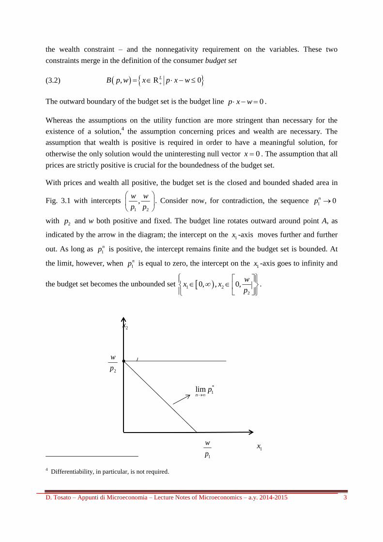
With prices and wealth all positive, the budget set is the closed and bounded shaded area in
Fig. 3.1 with intercepts 1 2
,w w
p p
. Consider now, for contradiction, the sequence 1 0np
with 2p and w both positive and fixed. The budget line rotates outward around point A, as
indicated by the arrow in the diagram; the intercept on the 1x -axis moves further and further
out. As long as 1
np is positive, the intercept remains finite and the budget set is bounded. At
the limit, however, when 1
np is equal to zero, the intercept on the 1x -axis goes to infinity and
the budget set becomes the unbounded set 1 2
2
0, , 0,w
x xp
.
4 Differentiability, in particular, is not required.
A
1
w
p
1x
2x
*
1limn
p
2
w
p
D. Tosato – Appunti di Microeconomia – Lecture Notes of Microeconomics – a.y. 2014-2015 4
Fig. 3.1 – Unboundedness of the budget set when 1p tends to zero
We conclude that the prices of all commodities must be positive in order that the budget set
be bounded and, therefore, compact. We can therefore assert that the Weierstrass Extreme
Value Theorem is applicable to our utility maximization problem since, by assumption, u x
is continuous and the budget set ,B p w is non empty, convex and compact.5 This
establishes the existence of a solution.
3.2. Utility maximization with only the wealth constraint
We begin with the simplest constrained optimization problem, that of maximizing the utility
function u x subject only to the wealth constraint. We suppose, in other words, that the
nonnegativity constraint on the variables may be, for the moment, disregarded on the tacit
assumption that the UMP has an internal solution, which excludes the possibility that the
quantity of one of the commodities is equal to zero. Taking furthermore into account the
assumption of monotone preferences, we can write the wealth constraint with the equality
sign, since the maximizing solution must necessarily occur on the boundary of the budget set,
that is on the budget line.
With these assumptions, the general utility maximization problem (3.1) reduces to the
following simpler problem
(3.4) max
subject to 0
xu x
p x w
The analytical techniques for determining the solution of an optimization problem involving
a twice continuously differentiable function, say f x , defined in the open domain int D a
subset of L , whether subject to constraints or not, goes through a first step consisting in
verifying the conditions for the existence of a solution, and a subsequent step consisting in the
determination of the necessary and sufficient conditions for an optimum, a maximum or a
minimum of f x .
We have already taken care of the first step, namely of the conditions for the application of
Weierstrass Extreme Value Theorem to the UMP, and concentrate, therefore, in this and in
5 Convexity of the budget set follows from the assumption that consumers operate in competitive markets where non
linear pricing policies are excluded
D. Tosato – Appunti di Microeconomia – Lecture Notes of Microeconomics – a.y. 2014-2015 5
the following sections on the second step that involves the determination of the first and
second order derivatives of f x . The first order conditions identify the critical points of the
function as the vector that solves the system of equations obtained by setting the first partial
derivative of the function equal to zero. The critical points may be maxima or minima or
saddle points. The second order condition distinguishes among these according to the
properties of the Hessian matrix of the second order derivatives, possibly on a proper
subspace of the domain.
3.2.1 First order necessary conditions
The standard approach to the solution of this optimization problem is to use the Lagrangean
method. The same result can actually be obtained by incorporating the wealth constraint in the
objective function, we call this for short the “substitution approach” as opposed to the
Lagrangean approach. We pursue first this alternative road, which has the advantage of
clarifying the connection between the second order conditions for a maximum and the
property of the utility function, and return subsequently to the formulation of the Lagrangean
function.
Solving the constraint, for instance, for Lx , we have
(3.5) 1
1 1
1
,..., ;L
lL L L l
lL L
pwx x x x w x
p p
Substituting for Lx from (3.5) in u x we obtain a new function of only 1L :
1 1 1 1 11 ,...,, ; ,.... .,. , L LL Lx x x w x xh x h x x h . Taking derivatives with respect to the
1L commodities, we obtain, for the generic commodity l , the following first order
condition for a critical value of v x
(3.6) * * * *
1 1,...,0
L lL
l l L l l L L
u x u x u x u xv x x px
x x x x x x p
where *x is the solution vector. We can rewrite (3.6) as
(3.7) * *
/ / ll L
l L L
u x u x pMRS
x x p
for all 1,..., 1l L
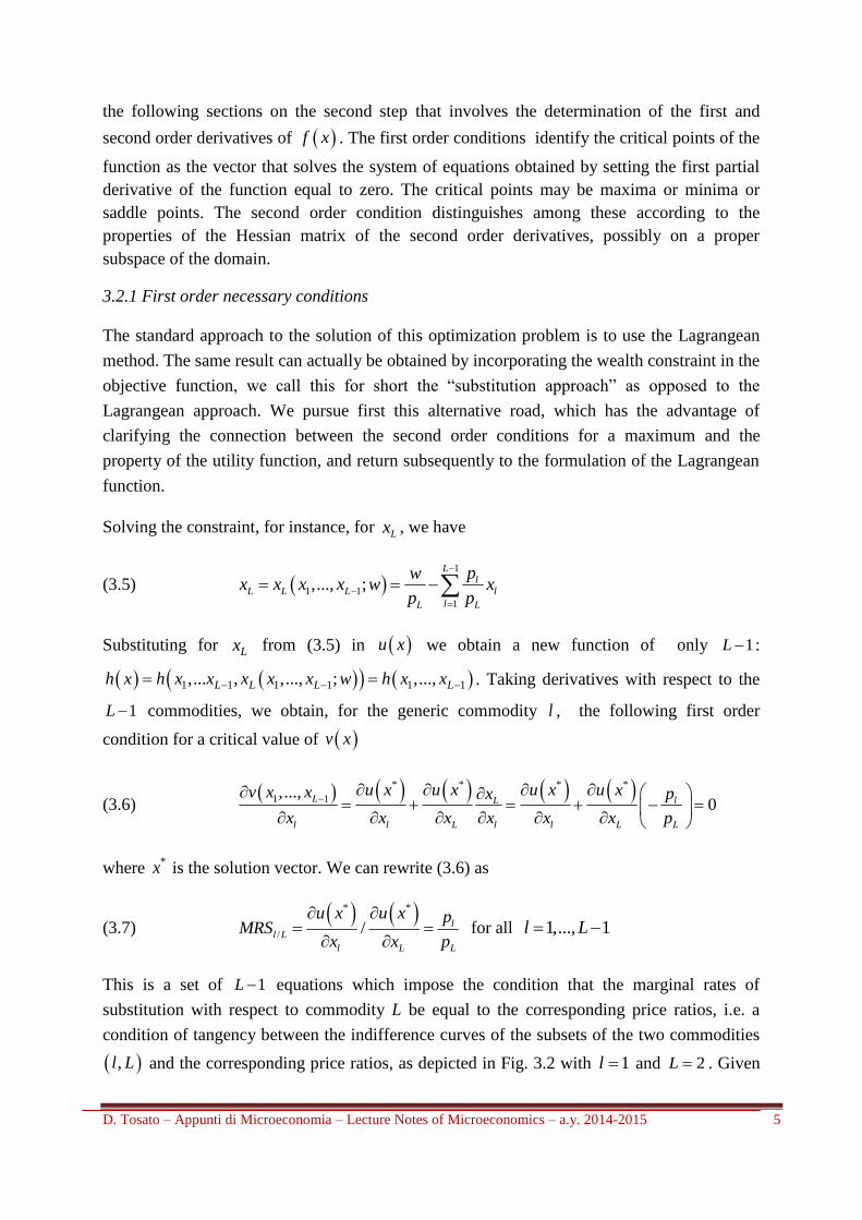
This is a set of 1L equations which impose the condition that the marginal rates of
substitution with respect to commodity L be equal to the corresponding price ratios, i.e. a
condition of tangency between the indifference curves of the subsets of the two commodities
,l L and the corresponding price ratios, as depicted in Fig. 3.2 with 1l and 2L . Given
D. Tosato – Appunti di Microeconomia – Lecture Notes of Microeconomics – a.y. 2014-2015 6
the assumptions made at the beginning of Section 3.1, strengthened to strict convexity of
preferences, the system of equations (3.7) has a unique solution; substituting in (3.5) also Lx
can be determined.
Consider now Lagrange’s method of analyzing the problem of utility maximization under
constraint, which consists in transforming the constrained optimization problem (3.4) into an
unconstrained one by adding a new variable the Lagrangean multiplier .6 In setting up the
Lagrange’s function care must be taken that, in the solution, the multiplier be of the right sign:
it should indicate the direction of change of the value function of the problem resulting from
an increase of wealth, i.e. from a relaxation of the constraint. To this end, we follow the
convention to set up the constraint in the “less than or equal” form and the multiplier with a
minus sign; alternatively, the constraint can be equivalently written in the “greater than or
equal” form and the multiplier with a plus sign. The Lagrangean is accordingly
(3.8) ,L x u x p x w
The critical points of the Lagrangean are determined by the condition that the partial
derivatives with respect to the variables x and be equal to zero. We have
(3.9)
* *
*
,0
,0
L xu x p
x
L xp x w
where * *,x is the solution of this set of equations.7
Lagrange’s theorem establishes that, if *x maximizes u x subject to the wealth constraint,
than there exists a unique number * that satisfies the set of equations in the first line of
(3.9).8 Note that
* is certainly positive because, even in the case, to be later examined, of a
boundary solution and given that we have assumed that all prices and wealth are strictly
positive, at least one of the elements of the vector *x must be positive, so that the
corresponding condition in the first line of (3.9) must be satisfied with the equal sign.
The economic meaning of the multiplier follows directly from the fact that wealth
represents the binding constraint on the utility level that can be achieved. A softening of the
6 Lagrange’s theory of constrained optimization is contained in his Lecons sur le calcul des functions (1806).
7 As we will argue in the Appendix A.3.2, it would not be correct to say that the solutions values * *,x are the
maximizers of the Lagrangean function (3.8). 8 For a proof of Lagrange’s Theorem see Appendix 3.A. See also MWG, pp. 956-7 and JR, pp. 577-601. A very simple
proof for the two-commodity case is offered by Simon-Blume, pp. 413-415.
D. Tosato – Appunti di Microeconomia – Lecture Notes of Microeconomics – a.y. 2014-2015 7
constraint, that is an increase in wealth, makes it possible to reach a higher indifference curve,
as in Fig. 3.2. The positive value of * measures, therefore, the marginal increase in utility
that the consumer can attain thanks to a differential increase in wealth, namely the marginal
utility of wealth.9 A word of caution about the numerical value of
* is in order. Since the
utility function representing preferences is defined up to an increasing monotonic
transformation, * measures the marginal utility of wealth with reference to the specific
utility function chosen in the class of function representing given preferences.
Fig. 3.2 – Effect of a wealth increase
3.2.2 Second order necessary conditions
Let us turn to the second order necessary condition for a maximum. Following the approach
already used, we first consider the “substitution approach” to utility maximization. Differently
from what we have done in the preceding Section, we focus, however, for ease of derivation
on the two commodity case; the extension to the case of more than two commodities is
straight forward.
9 As shown in appendix A.3.2, this is in effect the minimum value assigned to the marginal utility of wealth.
D. Tosato – Appunti di Microeconomia – Lecture Notes of Microeconomics – a.y. 2014-2015 8
Substituting for commodity 2 in terms of commodity 1, as indicated in (3.5) above, in the
utility function u x , we can reduce the problem of maximization under constraint to the
problem of unconstrained maximization of the following function of the single variable 1x
10
(3.10) 11 1 1
2 2
,pw
h x u x xp p
Taking first and second order derivatives of 1h x we have
(3.11) 11 1 1 2 1
2
ph x u x u x
p
(3.12)
1 1 11 11 1 12 1 21 1 22 1
2 2 2
2 2 *
2 11 1 2 12 1 222 2
2 2
1 1 2 det B
p p ph x u x u x u x u x
p p p
p u p p u p u H xp p
where first and second order partial derivatives of u x refer in proper order to the
derivatives with respect to the first and the second argument of the function 1h x and
*BH x is the 3x3 matrix in which the Hessian matrix of the utility function u x is
bordered with the price vector
(3.13) 11 12 1
*
21 22 2
1 2 0
B
u u p
H x u u p
p p
As will be shown in the Appendix, Section A.3.2 this is the Bordered hessian of the
Lagrange’s function.
The first and second order necessary conditions for a maximum are then, respectively,
1 0h x , which implies the equality between the marginal rate of substitution and the price
ratio
(3.14)
1 1
2 2
u x p
u x p
10 The approach followed here parallels the technique used in Lecture Note 2 to exemplify the notion that a negative
semidefinite matrix of a function of several variables is the analogue of a nonpositive second order derivative for a
function of a single variable.
D. Tosato – Appunti di Microeconomia – Lecture Notes of Microeconomics – a.y. 2014-2015 9
and 1 0h x , which implies that 1h x is negative (nonpositive) if and only if *BH x is
negative semidefinite, that is if *det BH x is positive (nonnegative).11
This last statement
means that H x is negative semidefinite in the linear space defined by the wealth constraint.
This conclusion establishes a direct connection between the second order necessary
conditions for a maximum and the properties of the utility function. In order to better pursue
this connection, let us first note that the matrix *BH x is similar to, but is not the Bordered
Hessian *BH x of the utility function u x , since the borders of the matrix *BH x are not
the partial derivatives of u x . In fact *BH x is
(3.15) 11 12 1
21 22 2
1 20
B
u u u
H x u u u
u u
But note - and this is the relevant point here - that given the direct proportionality between
the price vector p and the vector of partial derivative *u x , the determinant of *BH x is
just proportional to the determinant of *BH x .
As we have seen in Lecture Note 2, the utility function u x is quasiconcave if the Hessian
matrix of second order derivatives of u x is negative semidefinite in the linear subspace
0LZ z u x z . To grasp the implications of this condition, we make as usual
reference to the two variable case and reproduce below Fig. 2.7 of Lecture Note 2,
renumbered as Fig. 3.3.
11 See Lectue Note 2, Section 2.3.B.1.
D. Tosato – Appunti di Microeconomia – Lecture Notes of Microeconomics – a.y. 2014-2015 10
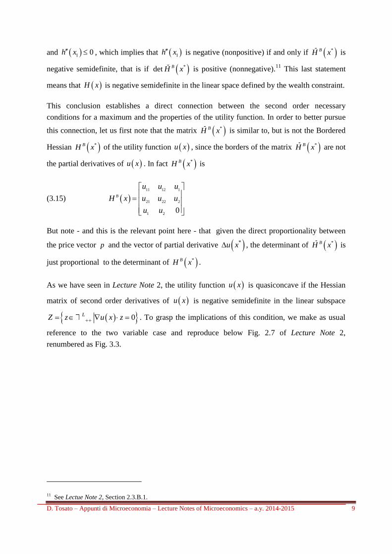
Fig. 3.3 – Quasiconcavity of u x on the wealth constraint
The line AB is now the wealth constraint * 0p x w tangent to the highest attainable level
curve of u x at the point *x . Consider an arbitrary small change x about *x , with the
vector 2x and
* 2x x , satisfying the wealth constraint, so that we have
0p x . Substituting the first order conditions for a maximum 1
* *p u x
and,
eliminating * 0 , we have * 0u x x . Noting that x stands for the vector z in the
Definition 2.10 of a quasiconcave function given in Lecture Note 2 the connection between
the definition of quasiconcavity of the utility function and the second order necessary
condition for a maximum is established.12
The second order sufficient condition for a maximum is 1 0h x for 1 0x . The difference
between second order necessary and sufficient conditions is illustrated in the appendix A.3.1
while the analytics of the determination of the second order conditions for a maximum
following the Lagrangean approach is postponed to Appendix A.3.2.
Appendix A.3.1 provides an analytical explanation of the role of the first and second order
necessary conditions in the determination of the maximizers of the utility function. We look
here for an intuitive explanation using economic considerations that can be easily drawn from
the diagram of Fig. 3.2. With u x representing monotone and convex preferences, it is
obvious that an internal solution, as assumed, must be represented by the tangency point
between the budget set and the highest indifference curve attained on the budget line.13
Points
12 This connection is further explored in Section 3.6.
13 We disregard here the possibility that the tangency point may occur on the coordinate axes.
D. Tosato – Appunti di Microeconomia – Lecture Notes of Microeconomics – a.y. 2014-2015 11
below the budget line are not maximizers, points above are unfeasible. The motivation for the
condition that the determinant of the bordered matrix *BH x , involving the Hessian of the
utility function, be negative semidefinite is, as explained in Lecture Note 2, a generalization to
the case of a vector variable of the condition of a non positive second order derivative in the
case of a scalar variable. Fig. 3.2 provides again the required intuition. A departure from the
tangency point, in the typical case of a strictly convex indifference curve, causes a movement
to a lower indifference curve and, therefore, a reduction in the utility level that could
otherwise be attained.
3.3. Maximization with only the nonnegativity constraint on the variables
Our next step is to study the problem of determining the conditions for the maximization of a
continuous twice differentiable function f x assuming that the only constraints on the
problem are represented by the nonnegativity condition on the vector of the choice variables
x . The problem is best examined if we consider that f x is a function of a single variable
and thus consider x a scalar. This has the advantage of explaining most clearly how we should
deal with a nonnegativity constraint, which may be binding or not, and of easily deriving the
consequent compact formulation of the first order conditions known as the Kuhn-Tucker
conditions. Although not formally specified by the Kuhn-Tucker conditions, the economic
meaning of the Lagrange’s multipliers of the nonnegativity constraints can be easily
identified. Again, the generalization to several variables does not present analytical
difficulties.
The maximization problem is now the following
(3.14) max
subject to 0
xf x
x
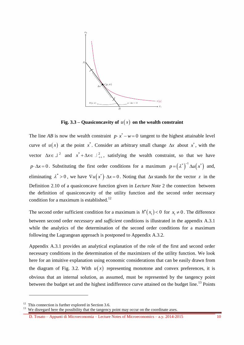
Fig. 3.4 shows the three possible situations that may arise. In Panel (a) the constraint is not
binding: the function f x attains its maximum at * 0x inside the feasible set; the interior
solution is then determined by the standard condition for an unconstrained problem *' 0f x
. In Panels (b) and (c) the optimal solution is on the boundary of the constraint set, at * 0x .
In Panel (b), the standard first order condition *' 0f x obtains, while in Panel (c) at * 0x
is associated the condition *' 0f x .
D. Tosato – Appunti di Microeconomia – Lecture Notes of Microeconomics – a.y. 2014-2015 12
Fig. 3.4 –Three possible maximizations with a nonnegativity constraint
An important fact emerges: in all three instances two conditions characterize now the optimal
solution: the first regarding the first order derivative, the second the value of the maximer.
Summing up in the order of three panels of Fig. 3.4, we have
(3.15)
* *
* *
* *
Panel a ' 0, 0
Panel b ' 0, 0
Panel c ' 0, 0
f x x
f x x
f x x
It is evident that these three cases can be synthesized into the following optimum conditions,
the Kuhn-Tucker conditions
(3.16)
*
* *
*
' 0
' 0
0
f x
x f x
x
or, disregarding the implicit condition that the optimal solution is nonnegative, in more
compact form
(3.17)
* *
* *
' 0 with equality if 0
' 0
f x x
x f x
We will for short, albeit somewhat improperly, refer in particular to the condition
* *' 0x f x in the second line of (3.17), which synthesizes the crucial aspect concerning the
presence of the nonnegativity constraints, as the Kuhn-Tucker condition.14
This is called the
complementary slackness condition.
14 Economists traditionally refer to the conditions of inequality constrained optimization problems – and, in particular,
to problems characterized by nonnegativity constraints on the choice variables – as the Kuhn-Tucker conditions, so
f(x)
x*
D. Tosato – Appunti di Microeconomia – Lecture Notes of Microeconomics – a.y. 2014-2015 13
The Lagrange’s function for the maximization problem (3.14) can now formulated following
the convention stated in the preceding Section on the utility maximization problem subject
only to the wealth constraint. Thus, also the nonnegativity the constraint must be set up in the
“less than or equal” form and the multiplier preceded by a minus sign. Using the Greek letter
for the multiplier of the nonnegativity constraint, the Lagrange’s function is
(3.18) ,L x f x x
The first order conditions for a critical value of ,L x with respect to the two variables x
and are
(3.19)
* *
* * * *
,0
,0 with the added slack condition =0 if >0, 0 if =0
L xf x
x
L xx x x
The added slack conditions can be formulated in the compact form
(3.20) * * 0x
which covers the three possible case of relation (3.15).
In the Kuhn-Tucker conditions (3.16) the multiplier * does not formally appear, but is
clearly implied by it. The Lagrangean formulation of the optimization problem subject to the
nonnegativity constraint clarifies the meaning of the expression complementary slack
condition. It states that if the constraint is slack, i.e. non binding and thus implying * 0x , the
multiplier must * be zero; if, on the contrary, the Lagrangean multiplier is strictly positive,
the constraint must be binding. This is exactly what the first order conditions (3.19) for a
critical value of ,L x say. Suppose that * 0x . Then from the second line of (3.19) we
know that * 0 and from the first line we have, therefore, *' 0f x . If, instead, the
constraint is strictly binding, then * 0 and in this case the first line of (3.19) is satisfied
with *' 0f x . The meaning of the positive value of the multiplier in this latter case is easily
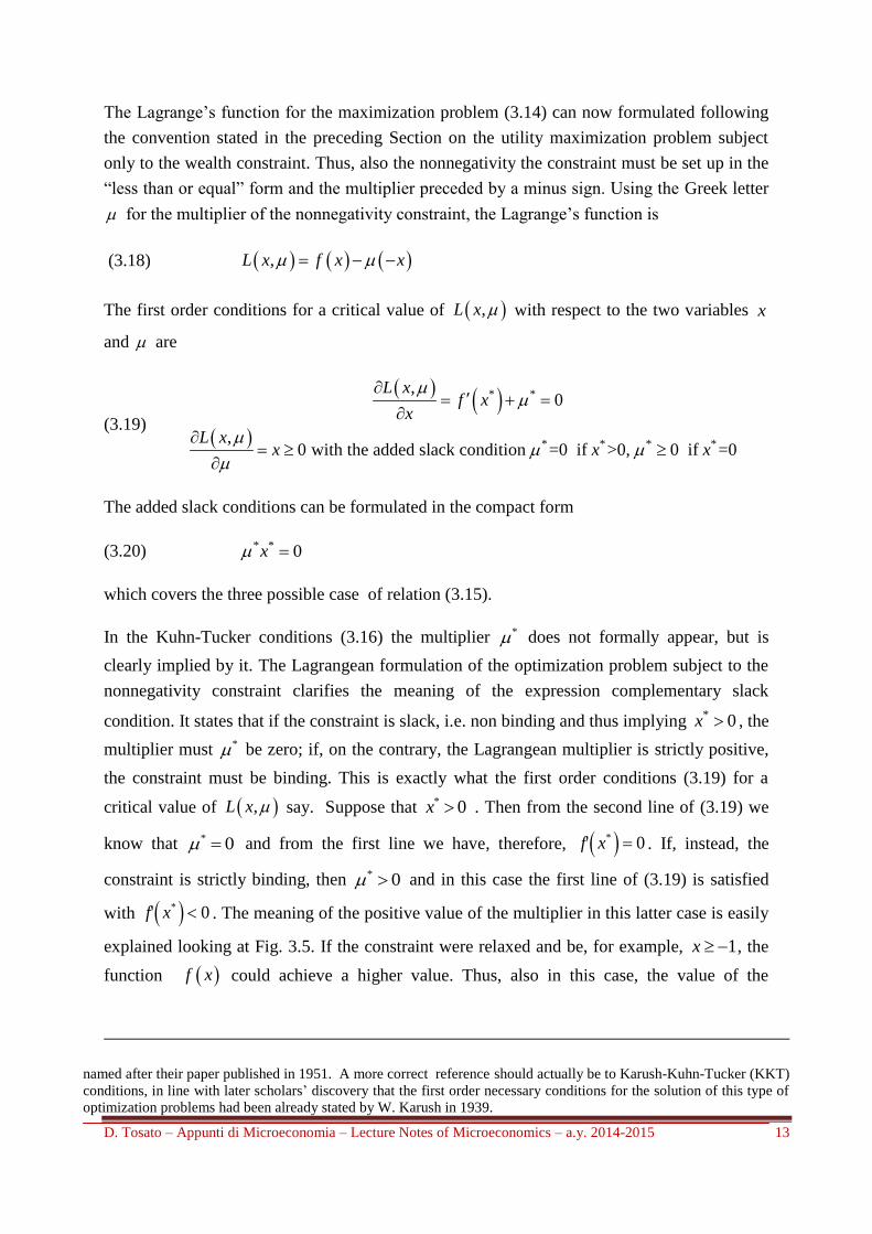
explained looking at Fig. 3.5. If the constraint were relaxed and be, for example, 1x , the
function f x could achieve a higher value. Thus, also in this case, the value of the
named after their paper published in 1951. A more correct reference should actually be to Karush-Kuhn-Tucker (KKT)
conditions, in line with later scholars’ discovery that the first order necessary conditions for the solution of this type of
optimization problems had been already stated by W. Karush in 1939.
D. Tosato – Appunti di Microeconomia – Lecture Notes of Microeconomics – a.y. 2014-2015 14
multiplier measures the benefit in terms of the optimal value of the objective function
deriving from a relaxation of the constraint.
Fig. 3.5 – Maximum of a function with a softening of the nonnegativity constraint
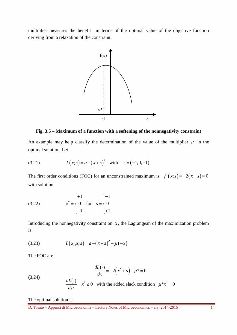
An example may help classify the determination of the value of the multiplier in the
optimal solution. Let
(3.21) 2
;f x s a x s with 1,0, 1s
The first order conditions (FOC) for an unconstrained maximum is ; 2 0f x s x s
with solution
(3.22) *
1
0
1
x
for
1
0
1
s
Introducing the nonnegativity constraint on x , the Lagrangean of the maximization problem
is
(3.23) 2
, ;L x s a x s x
The FOC are
(3.24)
*
* *
2 * 0
0 with the added slack condition * 0
dLx s
dx
dLx x
d
The optimal solution is
D. Tosato – Appunti di Microeconomia – Lecture Notes of Microeconomics – a.y. 2014-2015 15
(3.25)
* *
1,0
, 0,0
1, 2
x
for
1
0
1
s
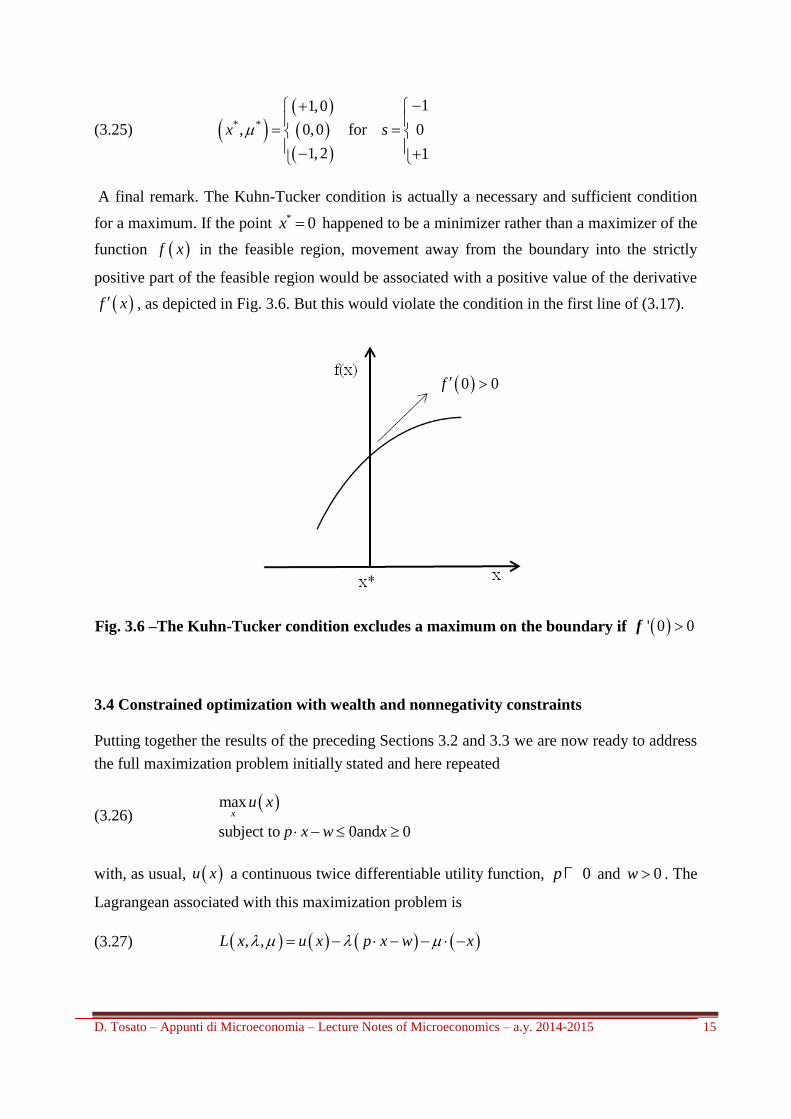
A final remark. The Kuhn-Tucker condition is actually a necessary and sufficient condition
for a maximum. If the point * 0x happened to be a minimizer rather than a maximizer of the
function f x in the feasible region, movement away from the boundary into the strictly
positive part of the feasible region would be associated with a positive value of the derivative
f x , as depicted in Fig. 3.6. But this would violate the condition in the first line of (3.17).
Fig. 3.6 –The Kuhn-Tucker condition excludes a maximum on the boundary if ' 0 0f
3.4 Constrained optimization with wealth and nonnegativity constraints
Putting together the results of the preceding Sections 3.2 and 3.3 we are now ready to address
the full maximization problem initially stated and here repeated
(3.26) max
subject to 0and 0
xu x
p x w x
with, as usual, u x a continuous twice differentiable utility function, 0p and 0w . The
Lagrangean associated with this maximization problem is
(3.27) , ,L x u x p x w x
0 0f
D. Tosato – Appunti di Microeconomia – Lecture Notes of Microeconomics – a.y. 2014-2015 16
Taking into account the fact that the wealth constraint is necessarily satisfied with the equal
sign, the critical values are determined by the following conditions
(3.28)
* * *
*
* * * * *
0
0
0 with the slack condition 0 if 0, 0 0
x
l l l l
LL u x p
x
Lp x w
LL x x if x
Using the Kuhn-Tucker conditions, the solution can be written in the compact form
(3.29)
* *
* * *
*
0
0
0
u x p
x u x p
p x w
It is worth looking with a little attention into the meaning of the multipliers of the
nonnegativity constrains, which can be retrieved from the slack conditions * * 0x ,
adapting to the context of the utility maximization problem the considerations made earlier. If
we have an interior optimum, i.e. if the variables are all strictly positive, the * ’s are all zero.
If we are, on the contrary, at a boundary solution, some * ’s may be equal to zero, but at least
one must be positive.
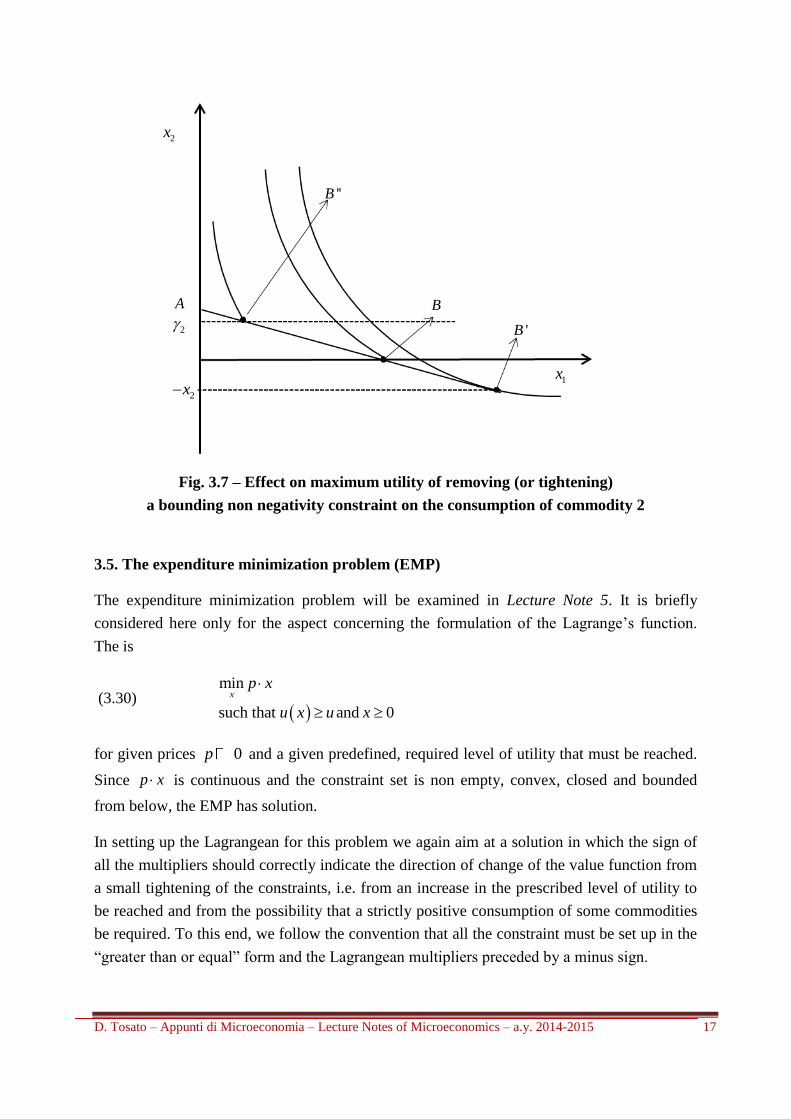
Consider the two commodity case and the boundary solution depicted by point B in Fig. 3.7,
where *
1 0x and *
2 0x . Note first that the tangency condition is not met, in fact, as
suggested by the diagram, the marginal rate of substitution is less than the price ratio. Note
second, concerning the role of the nonnegativity constraint, that if the constraint could be
relaxed to, say, 2 2x x , the optimal solution would occur on a higher indifference curve at
point 'B . A positive value of the multiplier signals the gain in utility obtainable from a
softening of the constraint. Note that the opposite would take place if we were to consider a
tightening of the constraint to 2 2x where
2 0 could represent a subsistence level, that
must be respected in the consumption of commodity 2.15
Utility maximization would in this
case occur on a lower indifference curve at point ''B in Fig. 3.7.
15 The Stone-Geary utility function reflects precisely this type of assumption and gives rise to the Linear Expenditure
System of demand functions (see R. Stone, 1954). The demand functions of Stone’s model are considered in Lecture
Note 4.
D. Tosato – Appunti di Microeconomia – Lecture Notes of Microeconomics – a.y. 2014-2015 17
Fig. 3.7 – Effect on maximum utility of removing (or tightening)
a bounding non negativity constraint on the consumption of commodity 2
3.5. The expenditure minimization problem (EMP)
The expenditure minimization problem will be examined in Lecture Note 5. It is briefly
considered here only for the aspect concerning the formulation of the Lagrange’s function.
The is
(3.30)
min
such that and 0
xp x
u x u x
for given prices 0p and a given predefined, required level of utility that must be reached.
Since p x is continuous and the constraint set is non empty, convex, closed and bounded
from below, the EMP has solution.
In setting up the Lagrangean for this problem we again aim at a solution in which the sign of
all the multipliers should correctly indicate the direction of change of the value function from
a small tightening of the constraints, i.e. from an increase in the prescribed level of utility to
be reached and from the possibility that a strictly positive consumption of some commodities
be required. To this end, we follow the convention that all the constraint must be set up in the
“greater than or equal” form and the Lagrangean multipliers preceded by a minus sign.
2
A
'B
B
2x
''B
2x
1x
D. Tosato – Appunti di Microeconomia – Lecture Notes of Microeconomics – a.y. 2014-2015 18
The Lagrangean of the problem is therefore16
(3.31) , ,L x p x u x u x
Taking account of the fact that the utility constraint is necessarily satisfied with the equal
sign, the critical values are determined by the following conditions
(3.32)
0
0
0 with the slack condition 0 if 0, 0 if 0
x
l l l l
LL p u x
x
Lu x u
LL x x x
Using the Kuhn-Tucker conditions, the solution can be written in the compact form
(3.33)
* *
* * *
*
0
0
0
p u x
x p u x
u x u
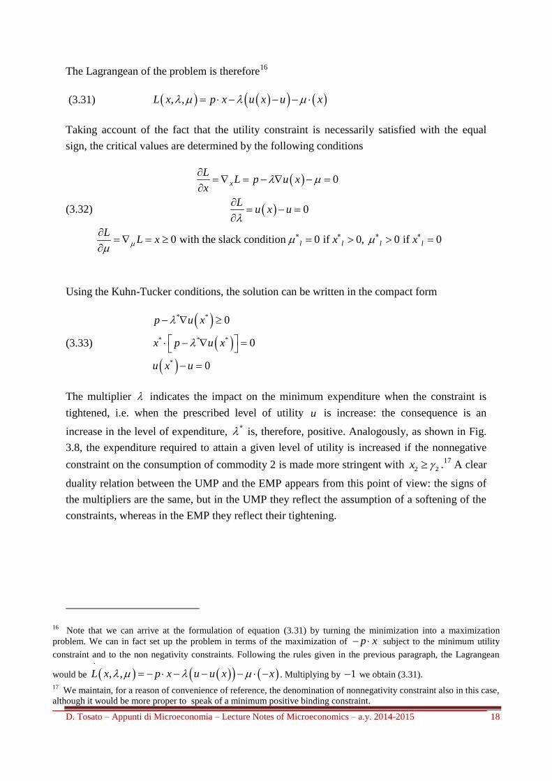
The multiplier indicates the impact on the minimum expenditure when the constraint is
tightened, i.e. when the prescribed level of utility u is increase: the consequence is an
increase in the level of expenditure, * is, therefore, positive. Analogously, as shown in Fig.
3.8, the expenditure required to attain a given level of utility is increased if the nonnegative
constraint on the consumption of commodity 2 is made more stringent with 2 2x .
17 A clear
duality relation between the UMP and the EMP appears from this point of view: the signs of
the multipliers are the same, but in the UMP they reflect the assumption of a softening of the
constraints, whereas in the EMP they reflect their tightening.
16 Note that we can arrive at the formulation of equation (3.31) by turning the minimization into a maximization
problem. We can in fact set up the problem in terms of the maximization of p x subject to the minimum utility
constraint and to the non negativity constraints. Following the rules given in the previous paragraph, the Lagrangean
would be , ,L x p x u u x x . Multiplying by 1 we obtain (3.31).
17 We maintain, for a reason of convenience of reference, the denomination of nonnegativity constraint also in this case,
although it would be more proper to speak of a minimum positive binding constraint.
D. Tosato – Appunti di Microeconomia – Lecture Notes of Microeconomics – a.y. 2014-2015 19
Fig. 3.8 – Effect on minimum expenditure of tightening a binding
nonnegativity constraint on the consumption of commodity 2
3.6 The role of concavity and quasiconcavity in optimization problems
The objective of this final Section is to state the relation between the second order conditions
for a maximum or a minimum which, as examined in Section 3.2 and in Appendix A.3.2, take
the form of properties of appropriate Hessian or Bordered Hessian matrices, with the notions
of concavity (convexity) and quasiconcavity (quasiconvexity) defined in Section 2.2 of
Lecture Note 2 precisely in terms of those matrices.
Let us first consider an unconstrained optimization problem. Given a generic twice
differentiable function f x , assume that the vector x , not necessarily unique, solves the
first order conditions * 0f x and determines, therefore, the critical points which may be
maxima or minima or saddle points. The second order condition distinguishes among these as
follows
(3.34)
a maximum negative semidefinite
* is a minimum if * is positive semidefinite
a saddle point indefinite
x H x
where *H x is the Hessian matrix of the function f x evaluated at *x . Taking account of
the properties of concavity and convexity of the function f x we can, therefore, conclude
with the following proposition.
2x= 2
u x u
2 2( , ;e p u x
)
2, ; 0e p u x
D. Tosato – Appunti di Microeconomia – Lecture Notes of Microeconomics – a.y. 2014-2015 20
Proposition 3.1 Let f x be a twice continuously differentiable function on LD ,
then x in the interior of D
(i) is a maximum if * 0f x and f x is concave;
(ii) is a minimum if * 0f x and f x is convex.
Furthermore:
(i) if * 0f x and f x is strictly concave, then x is a maximum of f x ;
(ii) if * 0f x and f x is strictly convex, then x is a minimum of f x .
It is, incidentally, worth noting that Definition 2.9 of Lecture Note 2 of a concave function has
an important implication for the identification of the properties of the solutions of a
maximization problem. We state this as a corollary.
Corollary 3.1. If f x is a twice continuously differentiable concave function18
on
LD and x in the interior of D is a local maximum, then for inty x D
(3.35) 0 implies f x y x f y f x
If (3.35) is verified for all inty D , then x is a global, not necessarily unique,
maximizer of f x .
A similar Corollary follows from the definition of a twice continuously differentiable convex
function simply turning the sign “ “ into the sign “ “.
Let us turn to a constrained optimization problem. The second order condition involves now
the properties of the Hessian matrix on the subspace LZ determined by the constraints
imposed to the optimization problem. The second order condition distinguishing among
maxima, minima and saddle points is as follows
(2.36)
a maximum negative semidefinite
* is a minimum if * is positive semidefinite in the subspace
a saddle point indefinite
Lx H x Z
Connecting finally the second order conditions just stated to quasiconcave and quasiconvex
functions, we may conclude with the following proposition.
18 Actually, the result holds for a
1C .
D. Tosato – Appunti di Microeconomia – Lecture Notes of Microeconomics – a.y. 2014-2015 21
Proposition 3.2 Let f x be a twice continuously differentiable function on LD ,
then x in the interior of D
(i) is a maximum if * 0f x and f x is quasiconcave;
(ii) is a minimum if * 0f x and f x is quasiconvex.
Furthermore:
(i) if * 0f x and f x is strictly quasiconcave, then x is a maximum of f x ;
(ii) if * 0f x and f x is strictly quasiconvex, then x is a minimum of f x .
D. Tosato – Appunti di Microeconomia – Lecture Notes of Microeconomics – a.y. 2014-2015 22
Appendix A.3 The analytics of the utility maximization problem
Appendix 3.A.1 Unconstrained optimization. At the end of Section 3.2 an intuitive
explanation, based on economic considerations, was given regarding the role of the first and
second order necessary condition for the determination of a maximizing solution. As
anticipated, we provide here an analytical explanation with reference to the very simple one
variable no constraint case.19
. In order to clarify the distinction between second order
necessary and sufficient conditions for a maximum, we consider
Let ;f x be a twice continuously differentiable function of the scalar variable x .
Suppose that *x is a local maximizer of f x ; suppose in other words that there exists an
open neighborhood of *x , say A , such that for all small arbitrary deviations
*z x x about *x in any direction, we have
(A3.1) * *f x f x z
Expanding the function on the right hand side of (A3.1) in a second order Taylor’s series
about the point *x (where 0z ) and disregarding higher order terms, which for z small will
be dominated by the quadratic term, we have
(A3.2) 2
* * * * 2
2
1
2
df d ff x z f x x z x z z
dx dx
with 0 1 . Substituting in (A3.1) we obtain the inequality
(A3.3) 2
* * 2
2
10
2
df d fx z x z z
dx dx
which must hold for any arbitrary small variation z .
By dividing both sides by z and taking the limit as z approaches zero, we have
(A3.4)
*
*
z 0 0
z 0 0
dfif x
dx
dfif x
dx
19 We follow here Intrilligator’s (2000), pp. 22-25) presentation and reproduce his illuminating diagram.
D. Tosato – Appunti di Microeconomia – Lecture Notes of Microeconomics – a.y. 2014-2015 23
Since the fundamental inequality (A.3.3) must be satisfied for all small arbitrary deviations z ,
we must have, as a first order necessary condition, that the first derivative of the function be
equal to zero at the local maximum
(A3.5) * 0df
xdx
Turning to the second order condition, we can first argue by exclusion. Using the first order
condition (A3.5), we can rewrite (A.3.2) as
(A3.6) 2
* * * 2
2
1
2
d ff x z f x x z z
dx
Since 2z is always positive, it follows that if the second order derivative 2
*
2
d fx z
dx is
positive, there exists z , in the small neighborhood A of *x , for which
* * 0f x z f x , contradicting the assumption that *x is a maximizer. We conclude that
for *x to be a local maximizer of f x the second order derivative must be negative or zero,
namely
(A3.7) 2
*
20
d fx
dx
Conditions (A3.5) and (A3.7) are then the first and second order necessary conditions for a
local maximum at *x .
20
The extension of the unconstrained optimization to the case of a vector variable Lx can
be analyzed with a similar procedure. Suppose that *x is a local maximizer of f x and let
Lz be a small arbitrary deviation about *x . We have
(A3.8) * *f x f x hz
with h an arbitrary small positive number. Expanding the right hand side of (A.3.9) in a
Taylor series about the point 0h , we obtain
(A3.9) * * * *1
2f x hz f x h f x z hz Hf x hz hz
20 The same result could have been reached using in (A3.2) the first order condition and taking account of the fact that 2z is always positive. The same approach is used by MWG(p. 933) to show that a function of a vector variable is
concave if and only if the Hessian matrix is negative semidefinite.
D. Tosato – Appunti di Microeconomia – Lecture Notes of Microeconomics – a.y. 2014-2015 24
where *f x is the vector of partial derivatives of the function, which must be equal to zero
for a critical point of the function, and *Hf x hz the Hessian matrix of f x , which
must the negative semidefinite for a maximum.
Suffient conditions for a strict local maximum at *x are, in the scalar variable case, that the
first derivative vanishes and, in particular, that the second order derivative be negative for all
*x x .21
The second order sufficient condition for a maximum is therefore
(A3.10) 2
*
20
d fx
dx
Give the stationarity condition (A3.5), changing the sign in relations (A3.7) and (A3.8) from
less than or equal to greater than or equal and from less than to greater then we obtain the
second order necessary and sufficient conditions of a local minimum.
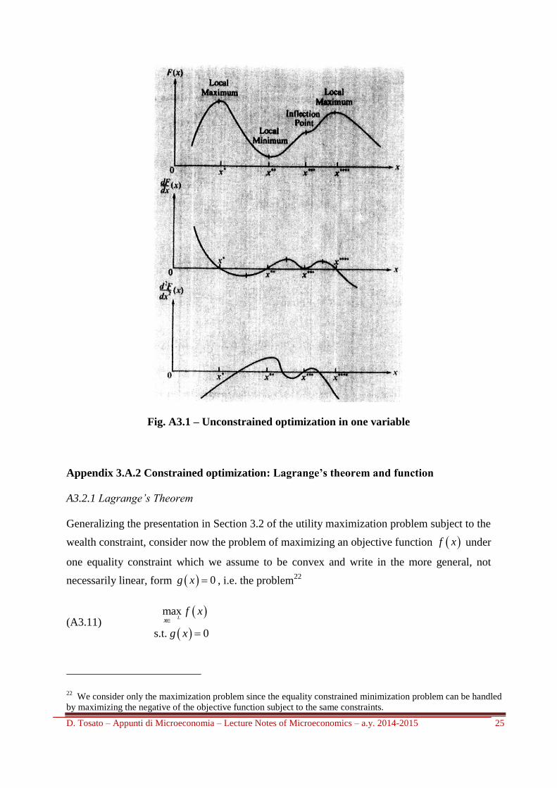
Fig. A3.1 in which the diagrams of the three functions: 2
2, and
df d ff x x x
dx dx are
depicted one below the other, illustrates the difference between necessary and sufficient
second order conditions:
the points *x and
****x are both strict local maxima: the first derivative vanishes and the
second derivative is negative;
the point **x is a strict minimum: the first derivative vanishes and the second derivative is
positive;
the inflexion point ***x is the crucial one for our purpose: the first order condition of zero
slope is met, but the second order derivative is also equal to zero, but changing sign from
negative to positive as we depart from ***x . The sufficient condition for a local maximum is
not met. This shows that the first and second order necessary conditions for a maximum are
not sufficient; they, in effect, coincide with the analogous first and second order conditions
for a minimum. A horizontal inflection point as ***x sign is neither a local maximum, nor a
local minimum.
21 In the vector variable case the second order sufficient condition is that Hessian be negative definite.
D. Tosato – Appunti di Microeconomia – Lecture Notes of Microeconomics – a.y. 2014-2015 25
Fig. A3.1 – Unconstrained optimization in one variable
Appendix 3.A.2 Constrained optimization: Lagrange’s theorem and function
A3.2.1 Lagrange’s Theorem
Generalizing the presentation in Section 3.2 of the utility maximization problem subject to the
wealth constraint, consider now the problem of maximizing an objective function f x under
one equality constraint which we assume to be convex and write in the more general, not
necessarily linear, form 0g x , i.e. the problem22
(A3.11)
max
s.t. 0
Lxf x
g x
22 We consider only the maximization problem since the equality constrained minimization problem can be handled
by maximizing the negative of the objective function subject to the same constraints.
D. Tosato – Appunti di Microeconomia – Lecture Notes of Microeconomics – a.y. 2014-2015 26
Following the approach of Section A3.1, let ; Lf x be a twice continuously
differentiable function of the vector variable x . Suppose that *x is a local maximizer of
f x subject to the twice differentiable and convex constraint 0g x ; suppose in other
words that there exists an open neighborhood of *x , say LA , such that for all small
arbitrary deviations * Lz x x about
*x in any direction, we have
(A3.12) * *f x f x hz
with h an arbitrary small positive number. Expanding the right hand side of (A.3.12) in a
Taylor series about the point 0h , we obtain
(A3.13) * * * *1
2f x hz f x h f x z hz Hf x hz hz
where *f x is the vector of partial derivatives, which must be equal to zero for a critical
point of the function, and *z Hf x z is a quadratic form, which must be negative
semidefinite (negative definite) for a maximizing solution.
As we have seen in Lecture Note 2, Section 2.2, the presence of a constraint requires that the
properties of the Hessian Hf x be evaluated on the subspace * 0LZ z f x z .
We have shown in Section 3.2 above that this property is verified in the utility maximization
problem by a particular Bordered Hessian, namely by the Hessian of u x bordered by the
vector of commodity prices, which define the slope of the tangent line to the indifference
curve at *x . In order to better understand the meaning of these particular bordering elements it
is useful to take into consideration a somewhat more general constrained maximization
problem. We suppose, in fact, that the constraint need not be necessarily linear, as the wealth
constraint is, but that it may be strictly convex.
The plan of this Section is to state first, without proof, Lagrange’s theorem: We then show:
(i) that the critical values of the Lagrangean function * *,x do satisfy the conditions for *x
to be a maximizer of f x subject to the constraint 0g x ; and (ii) that the Bordered
Hessian *BH x , defined in (3.13), of the utility maximization problem under the wealth
constraint is just a particular case of the more general problem of maximization under a
convex constraint.
D. Tosato – Appunti di Microeconomia – Lecture Notes of Microeconomics – a.y. 2014-2015 27
We will go back later to the linear form of the wealth constraint to establish the connection
with the presentation in Section 3.2; we maintain the assumption of the existence of an
internal solution and disregard the nonnegativity constraints on the variables. The approach
may be extended to the consideration of a set of M constraints with L M for, otherwise, the
constraint set will in general be empty.23
The feasible point *x C is a local maximizer of f x if that there exists an open
neighborhood of *x , say LA , such that *f x f x for all x A C ;
*x is a global
maximizer of f x if *f x f x for all Lx .
Lagrange’s Theorem. Let: (i) the objective function f x and the constraint function
g x be twice continuously differentiable and increasing in x; (ii) *x be an interior
solution of the optimization problem (A3.11); (iii) the vector of partial derivatives of the
constraints is positive, 0f x . Then there is a positive number * , the
Lagrangean multiplier of the constraint, such that
(A3.14) * *
* 1,...,l l
f x g xl L
x x
or in vector form notation
(A3.15) * * *f x g x
In words, the gradient vector of the objective function is proportional to a linear combination
of the gradient vector of the constraint function.24
We refer for a proof of Lagrange’s theorem to the references indicated in footnote 23 and
pass directly to an examination of Lagrange’s function and its properties.
The Lagrange’s function associated to the maximization problem (A.3.11) is
(A3.16) ,L x f x g x
23 For the more general approach, in particular for the case of two constraints and the relative graphical
presentations see MWG (pp. 956-9963), JR (pp. 577-601), Intrilligator (pp. 28-38). 24
The extension to the case of 1M constraints requires to introduce the constraint qualification, namely the
condition that the Jacobian matrix M N be of rank M . In this case, Lagrange’s theorem asserts the existence of a
vector of M positive multipliers, one for each constraint, such that the gradient vector of the objective function is
equal to a linear combination of the gradient vectors of the constraint functions.
D. Tosato – Appunti di Microeconomia – Lecture Notes of Microeconomics – a.y. 2014-2015 28
The critical values * *,x are the solutions of the 1L first order conditions
(A3.17)
* * *
*
, 0
, 0
xL x f x g x
L x g x
The L equations of the first line of (A3.17) exactly coincide with (A3.15). The fundamental
result of Lagrange’s Theorem is immediately verified by the first order conditions of the
associated Lagrangean function.
There remains to ascertain that the critical values *x of the Lagrangean function do maximize
the objective function f x subject to the constraint.
At the critical values * *,x the Lagrangean function ,L x must be stationary; this
implies that the total differential dL must be equal to zero
(A3.18)
* *
* * *
1 1
, 0L L
l l
l ll l
f x g xdL x dx g x d dx
x x
Note first that the second term on the right hand side of (A3.18) vanishes because the critical
values *x satisfy the equality constraint - conditions (A3.17). Observe next that also the third
term on the right hand side of (A3.18) is equal to zero since the admissible deviations ldx in
the neighborhood of *x must satisfy the constraint, hence
*
1
0L
l
l l
g xdx
x
.
25 (A3.18) thus
reduces to
(A3.19) *
1
, 0L
l
l l
f xdL x dx
x
which insures that any arbitrary small deviation from the optimal solution *x does not
increase the value of the objective function.
We can now say a bit more about the nature of the critical values * *,x of the Lagrange’s
function. We can say that the maximum over the choice variable x of the objective function
f x subject to the equality constraint 0g x coincides with the unconstrained maximum
25 Going back to Section 3.2.2, in which the two variable one equality constraint case was studied, Fig. 3.3 shows
that the admissible deviations ldx must lie on the budget constraint.
D. Tosato – Appunti di Microeconomia – Lecture Notes of Microeconomics – a.y. 2014-2015 29
over x of the associated Lagrangean. We defer for the moment discussing the nature of the
Lagrangean multipliers * .
A3.2.3 Second order necessary conditions for a maximum
The study of second order necessary and sufficient conditions, already discussed in Section
3.2 with reference to the problem of utility maximization subject to the wealth constraint, can
now be extended to the case here considered of a twice differentiable equality constraint,
obviously maintaining the assumption that the objective function is quasiconcave and twice
differentiable. We now show that the second order condition derived using the substitution
approach to the constrained maximization of the utility function coincides with the Bordered
Hessian of the Langrage’s function.
Consider the two-commodity maximization problem
(A3.20)
2 1 2
1 2
max ,
s.t. , 0
xf x x
g x x
Following the “substitution” approach to the solution of the maximization problem, think of
the constraint as defining 2x in terms of 1x , namely 2 1x x . The slope of the constraint set is
(A3.21) 2 1
1 2
dx g
dx g
Substituting 2 1x x in the objective function, let
(A3.22) 1 1 2 1,h x f x x x
be the value of the objective function subject to the constraint. Differentiating 1h x with
respect to 1x and taking first and second order derivatives as we have done in Section 3.2, we
respectively have
(A3.23) 11 2
1 2
gdhh h
dx g
(A3.24)
21 1 1
11 12 21 2222 2 21
2 1 12 11 12 1 21 222
2 22
-
g g gd hf f f f
g g gdx
f g gg g g g g g
g gg
D. Tosato – Appunti di Microeconomia – Lecture Notes of Microeconomics – a.y. 2014-2015 30
The joint presence of the second order derivatives of the objective function and of the
constraint function does not permit of a direct interpretation of this expression, which
however becomes possible in connection with the introduction of the Lagrangean function
(A3.16). Given the first order conditions
(A3.25)
* * * * *1 1 1
* * * * *2 2 2
, 0
, 0
L x f x g x
L x f x g x
we can define the second order partial derivatives of ,L x at * *,x
(A3.26)
* * * * *11 11 11
* * * * * * *12 21 12 12
* * * * *22 22 22
,
, ,
,
L x f x g x
L x L x f x g x
L x f x g x
Substituting in (A3.24) first equations (A3.25) and subsequently the second order derivatives
(A3.26), we obtain
(A3.27)
2* 2 * * 2
11 11 2 12 12 1 2 22 22 12 21 2
2 211 2 12 1 2 22 12
2
12
1 = 2
d hf g g f g g g f g g
dx g
L g L g g L gg
The term in curly brackets is equal to the determinant of the matrix
(A3.28) 11 12 1
* *21 22 2
1 2
det ,
0
L L g
HL x L L g
g g
which is the Bordered Hessian of the Lagrangean function, namely the matrix of the second
order partial derivatives of ,L x bordered by the first derivatives of the constraint, all
evaluated at the critical values * *,x . We can conclude that the second order necessary
(sufficient) condition for a maximum is satisfied if the determinant of the bordered Hessian
* *,HL x is nonnegative (positive) for all *x x .
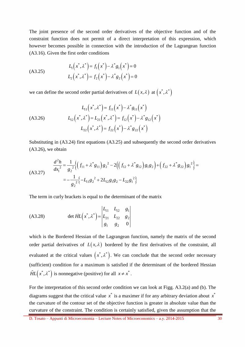
For the interpretation of this second order condition we can look at Figg. A3.2(a) and (b). The
diagrams suggest that the critical value *x is a maximer if for any arbitrary deviation about
*x
the curvature of the contour set of the objective function is greater in absolute value than the
curvature of the constraint. The condition is certainly satisfied, given the assumption that the
D. Tosato – Appunti di Microeconomia – Lecture Notes of Microeconomics – a.y. 2014-2015 31
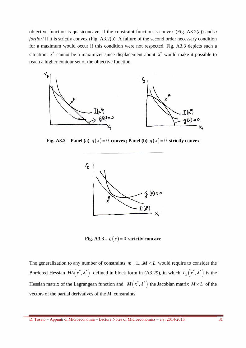
objective function is quasiconcave, if the constraint function is convex (Fig. A3.2(a)) and a
fortiori if it is strictly convex (Fig. A3.2(b). A failure of the second order necessary condition
for a maximum would occur if this condition were not respected. Fig. A3.3 depicts such a
situation: *x cannot be a maximizer since displacement about
*x would make it possible to
reach a higher contour set of the objective function.
Fig. A3.2 – Panel (a) 0g x convex; Panel (b) 0g x strictly convex
Fig. A3.3 - 0g x strictly concave
The generalization to any number of constraints 1,...m M L would require to consider the
Bordered Hessian * *,HL x , defined in block form in (A3.29), in which * *,llL x is the
Hessian matrix of the Lagrangean function and * *,M x the Jacobian matrix M L of the
vectors of the partial derivatives of the M constraints
D. Tosato – Appunti di Microeconomia – Lecture Notes of Microeconomics – a.y. 2014-2015 32
(A3.29)
* * * *
* *
* *
, ,
,
, 0
ll
T
L x M x
HL x
M x
and ascertain the conditions for it to be positive semidefinite (definite).26