Advanced Geophysical Interpretation Centre

3D modeling of the Quest Projects

Geophysical Datasets

Undercover Exploration workshopKEG-25 April 2012

Nigel Phillips

Mineral Physical Properties: density–sus. cross-plot

after Williams 2007

Rock Physical Properties: density–sus. cross-plot

after Williams 2007

What are the dominant causes of physical properties?

Mineralogy Texture

Grain size Porosity

Serpentinisation

Mineralisation

Igneousdifferentiation

Metamorphism

Weathering

Rock Physical Properties – Processes: density–sus. cross-plot

after Williams 2007

How do geologic processes change

physical properties?

Inversion Essentials: What is Inversion?

Inversionprocessing

Model Inversion estimates Earth models based upon

data and prior knowledge.

??

Data

Measurements over

the Earth are data.

source: UBC-GIF

Energy from source

Earth’sphysical properties

Measurements = Data

Pre-processing

Prior information

Inversion within it’s proper context …

Inversion.

Physical property

distributions = MODELS

Inversion Theory

Main objective:

Choose a model that emulates geology and fits the data,

but doesn’t fit the noise in the data.

2 Challenges:

There are an infinite number of possible models � non-uniqueness

How do we choose one?

We don’t know how noisy the data are.

Inversion Theory: Non-uniqueness

Why an infinite number of models?

The data (100’s – 100,000’s values) are not sufficient to uniquely determine 10,000,000’s earth model parameters.

� Under-determined problem.

The physical phenomena that we are exploiting (gravity, electromagnetic propagation) is usually a decaying as a function of depth or distance, and is not sufficient to uniquely describe the earth model.

Questions to consider:

Consider the simple problem that involves two unknowns (model parameters), x and y. We have one datum, 2.

x+y=2

What is the value of x and y?

� Infinite number of solutions

Consider some candidate models for the x and y parameters:

a: (0,2)

b: (1,1)

c: (2,0)

d: (-1,3)

Which one do we choose?

Using prior information to choose optimal models

Encode prior knowledge in a form that can be “optimized”.

i.e. build a mathematical rule or norm to test sizes of possible

models, then choose the “smallest”.

• The people-in-the-room analogy:

source: UBC-GIF

Questions to consider:

Consider the simple problem that involves two unknowns (model parameters), x and y. We have one datum, 2.

x+y=2

What is the value of x and y?

� Infinite number of solutions

Consider some candidate models for the x and y parameters:

a: (0,2) positive gradient

b: (1,1) flattest

c: (2,0) negative gradient

d: (-1,3) has smallest value

norms are described mathematically

How to pick one of infinitely many solutions?

Geophysical prior knowledge:

Values are positive, and/or within bounds

Physical Properties: Estimates for host rock properties

Point-location values from drill hole information

Logical prior knowledge:

Find a “simple” result - as featureless as possible.

This sacrifices resolution but prevents over-interpreting the data.

Geologic prior knowledge:

Character of the model (smooth, discontinuous)

Some idea of scale length (or size) of the bodies

Structural Constraints

Challenge: Describe geology mathematically

Narrow down the number of options using prior knowledge.

Questions to consider:

Consider the simple problem that involves two unknowns (model parameters), x and y. We have one datum, 2.

x+y=2

But we really have:

x+y=2 (+/- unknown error)

Sources of noise:

Instrument noise (sensitivity, accuracy, t0)

Location noise (GPS)

Geologic noise – near surface geology not of interest

Modelling errors – discretization limitations

Operator mistakes

Topography resolution

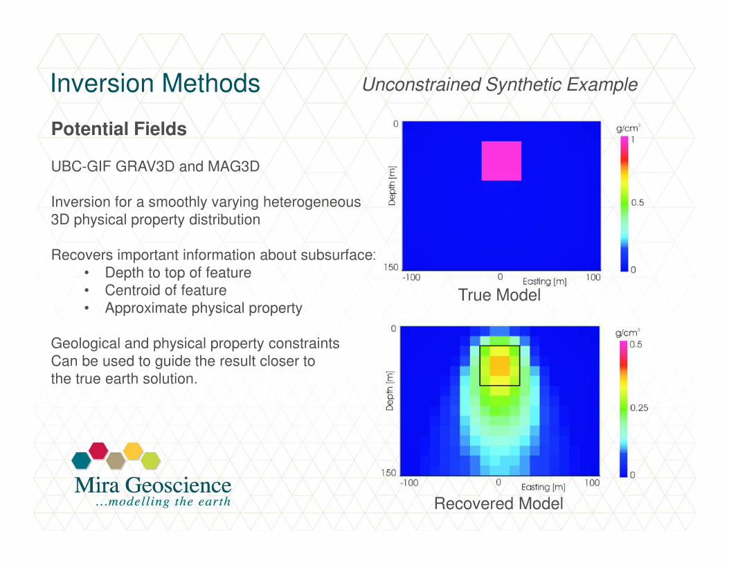
Inversion Methods

Potential Fields

UBC-GIF GRAV3D and MAG3D

Inversion for a smoothly varying heterogeneous

3D physical property distribution

Recovers important information about subsurface:

• Depth to top of feature

• Centroid of feature

• Approximate physical property

Geological and physical property constraints

Can be used to guide the result closer to

the true earth solution.

True Model

Recovered Model

Unconstrained Synthetic Example

Inversion Methods

Potential Fields

UBC-GIF GRAV3D and MAG3D

Inversion for a smoothly varying heterogeneous

3D physical property distribution

Recovers important information about subsurface:

• Depth to top of feature

• Centroid of feature

• Approximate physical property

Geological and physical property constraints

Can be used to guide the result closer to

the true earth solution.

Half of model constrained

���� improves other half

True Model

Recovered Model

Constrained Synthetic Example

Inversion models in contextGeophysical inversions are non-unique and generated from noisy data.

Be aware of this and use responsibly.

Logical (non-geologic) constraints are a good starting point and add value to the data.

Use prior information to further narrow down the range of suitable models.

Common Earth Models

Geologic models + Geochemical models + Geophysical models

Honour all the data provide the most comprehensive, quantitative view of the subsurface.

Modelling Objectives

• Provide useful 3D physical property products

• For direct employment in regional exploration

• Provide guidance to the regional structure

• Help geologic mapping

• Help target prospective geology, alteration, or mineralization.

• Exploration criteria for different styles of mineralization can be applied based

on multiple physical properties.

• Depth of overburden analysis

• Guide detailed follow-up survey design

Products

• 3D inversions of potential field data

• Interpolated 3D conductivity model based on 1D EM inversions

• Integrated 3D Physical Property Classification Models

• Accessible deliverables for visualization and quantitative 3D analysis

• Detailed infill areas

Mining Regions of BC and RegionalGeophysical Survey Coverage

Summary of data

• Sanders airborne gravity

• GSC gravity compilation

• (Geotech magnetic)

• Aeroquest magnetic

• GSC magnetic compilation

• Geotech VTEM data

• Aeroquest AeroTEM data

Gravity Data

Airborne acquisition by Sander Geophysics

East-West lines with 2000m line spacing

Regional GSC data also used for regional signal

mGal

Terrain Corrected

Bouguer Anomaly

(2.67 g/cm3)

Magnetic Data

Airborne acquisition by Geotech and Aeroquest

East-West lines with 4000m line spacing

Regional GSC data also used for regional signal

nT

Total Magnetic Intensity

Summary of ModelsFour large survey areas and 6 small infill areas:

Bell, Endako, Equity, Huckleberry, Granisle, and Morrison.

Potential Fields:

3D Density Contrast Model (UBC-GIF Grav3D)

3D Magnetic Susceptibility model (UBC-GIF Mag3D)

500m x 500m x 250m cells

Tiled inversions (full compilation = ~100 million cells)

Airborne EM

Late time conductivity map

3D (interpolated) conductivity model (UBC EM1DTM)

Depth of system penetration estimate

Conductive Plates (EMIT Maxwell)

GIS compilation in Gocad

0m elev.Density

Contrast

Model

g/cm3

-2000m elev.Density

Contrast

Model

g/cm3

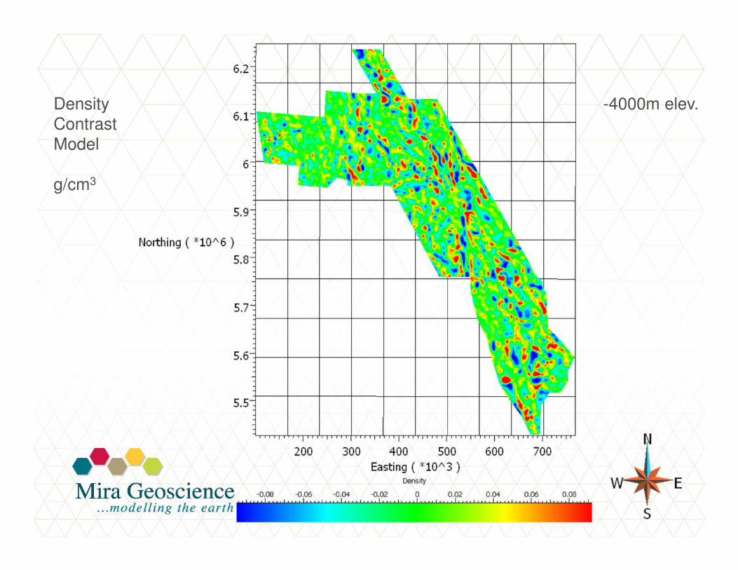
-4000m elev.Density

Contrast

Model

g/cm3

0m elev.Magnetic

Susceptibility

Model

S.I.

-2000m elev.Magnetic

Susceptibility

Model

S.I.

-4000m elev.Magnetic

Susceptibility

Model

S.I.

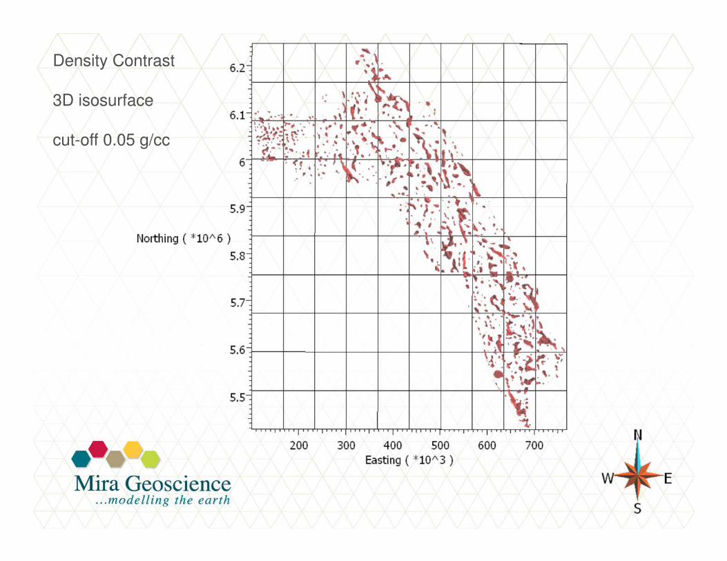
Density Contrast

3D isosurface

cut-off 0.05 g/cc

Magnetic susceptibility

3D isosurface

cut-off 0.05 S.I.

Prospective regions of

High density contrast

and high magnetic

susceptibility.

Airborne EM Modelling

1D Inversions

Inversion for a smoothly varying heterogeneous 1D conductivity distribution

Laterally Constrained� Inversion parameters are tuned to the changing geology

Background/Late-Time Conductivity

Depth of Investigation based on cumulative conductance

Plate Modelling

Alternative to the 1D interpretation for use when the layered earth assumption is inadequate.

Electromagnetic Data

Airborne acquisition by Geotech (VTEM system)

East-West lines with 4000m line spacing

Channel 19 dBz/dt data

27 time channels used

~78m flight height

nT/s

Inversion Methods

Airborne EM

UBC-GIF EM1DTM

Inversion for a smoothly varying heterogeneous

1D conductivity distribution

Laterally Parameterized/Constrained Inversion

Neighbouring stations used to determine

appropriate inversion parameters

Reduces modelling artefacts

Background/Late-Time Conductivity

Background Conductivity: Plan View

S/m

AeroTEM modelling:

Late-time Background Conductivity (Quest West)

Inversion Methods

Airborne EM

UBC-GIF EM1DTM

Inversion for a smoothly varying heterogeneous

1D conductivity distribution

Laterally Parameterized/Constrained Inversion

Neighbouring stations used to determine

appropriate inversion parameters

Reduces modelling artefacts

Background/Late-Time Conductivity

Depth of Investigation based on cumulative conductance

Conductivity Flight-line Section

Inversion Results

Airborne EMConductivity Model

Log conductivity [S/m]

Fences shown through full

3D conductivity model

Conformable with topography

Inversion Results

Log conductivity [S/m]

Airborne EM Conductivity ModelZoom

Fences shown through full

3D conductivity model

Conformable with topography

Using the Results

Quest Block C:

• Conductivity model: East-West flight line model sections

• Density Contrast iso-surface at a value of 0.05g/cm3

• North-South magnetic susceptibility section

AeroTEM modelling: Huckleberry Mine Infill Area

Stacked sections through 3D conductivity Model

AeroTEM modelling: Huckleberry Infill Area

AeroTEM modelling: Huckleberry Infill Area

Stacked sections through 3D conductivity Model

Conductivity Model - isosurfacesAeroTEM modelling: Huckleberry Infill Area

Conductivity Model - platesAeroTEM modelling: Huckleberry Infill Area

Inversion Results

Physical Property Classification

•Common 3D Discretization Mesh

•Each Physical Property classified into High, Medium, and Low

•Density Contrast and Magnetic Susceptibility

Two-phase system � 9 classifications

•Density Contrast, Magnetic Susceptibility, and Conductivity Background

Three-phase system � 27 classifications

Inversion Results

3D Physical Property

Classification

Surficial Plan View

of 3D classification model

Inversion Results

3D Physical Property

Classification

Surficial Plan View

of 3D classification model

Using the Results

• Regional Interpretation

• Integrated Interpretation

• Interpretation with Physical Properties

• Constraining Information

• Target Customization

• Survey Design

• Integrated Modelling

• Common Earth Model Development

• 3D GIS Regional Targeting

Qualitative

Quantitative

Using the Results

Evaluation of physical property classification based on known

mineral occurrences:

1. Compute spatial correlation of physical property classifications with known mineral occurrences in 3D.

2. Determine which class has the highest correlation.

3. Perform for Density Contrast and Magnetic Susceptibility two-phase system, and Density Contrast, Magnetic Susceptibility, and Conductivity Background three-phase system.

Using the Results – evaluation of physical property classification

Distance to known

mineral occurrences.

Using the Results – Den/Sus: Class 9

3D regions of interest

Using the Results – Den/Sus/Con: Class 9

3D regions of interest

Targeting Workflow

Establish clear exploration objectives and criteria

Target generation from the Common Earth Model

Target ListX Y Z3045 2465 10103456 4576 11453104 6543 12793303 4531 1109…

Mineral Potential Cube

Summary3D density contrast, magnetic susceptibility, and conductivity models have been produced.

The models provide more useful information than the data alone.

While being aware of the limitations, the models can be used to promote detailed follow-up through 3D-GIS targeting analysis.

The infill areas provide examples of what information can be extracted from these

data.

Introduce new information as it is acquired to test the validation of these models, and to help improve upon them as more focussed targets are resolved.

Acknowledgements

Geoscience BC

Team of Geophysicists at Mira Geoscience Advanced Geophysical Interpretation Centre

UBC-GIF