Boise State UniversityScholarWorks

Computer Science Graduate Projects and Theses Department of Computer Science

4-1-2015

Accelerated Radar Signal Processing in LargeGeophysical DatasetsRavi Preesha GeethaBoise State University

Geophysics research involves the study of geophysical events with the help of large amounts of data collected from instruments such as radars, deployedon the ground, aircraft and satellites. Radar signal processing applications analyze radar sensor data to estimate material properties of the subsurface.The amount of data generated is increasing exponentially as hardware improves and more observations are being captured to make accurate predictions.However, the speed of signal processing algorithms has not kept pace with increase in measurement speed making the processing techniques lessefficient and time consuming.In this project a parallel radar signal processing algorithm for snow depth estimation was implemented using the Hadoop framework. This will enableresearchers to effectively execute the processing algorithm on existing massive datasets using Hadoop in the near future, and also use Hadoop as areliable and stable storage system for the large files generated by the algorithm.To find the efficiency and accuracy of the parallel processing algorithm, experiments were executed on datasets ranging from 0.5GB to 4GB on aHadoop cluster. The results demonstrated that Hadoop can process the radar signals on large data sets much faster than the currently used sequentialsignal processing algorithm implemented in MATLAB and can store result files generated by the algorithm more efficiently. The Hadoop algorithm wasalso deployed on a High Performance Computing cluster to identify the challenges in running in a cluster environment that uses traditional batch jobsystems.

ACCELERATED RADAR SIGNAL PROCESSING IN LARGE

GEOPHYSICAL DATASETS

by

Ravi Preesha Geetha

A project

submitted in partial fulfillment

of the requirements for the degree of

Master of Science in Computer Science

Boise State University

April 2015

c© 2015Ravi Preesha Geetha

ALL RIGHTS RESERVED

BOISE STATE UNIVERSITY GRADUATE COLLEGE

DEFENSE COMMITTEE AND FINAL READING APPROVALS

of the project submitted by

Ravi Preesha Geetha

Project Title: Accelerated Radar Signal Processing in Large Geophysical Datasets

Date of Final Oral Examination: 29 April 2015

The following individuals read and discussed the project submitted by student Ravi PreeshaGeetha, and they evaluated their presentation and response to questions during the final oralexamination. They found that the student passed the final oral examination.

Amit Jain Chair, Supervisory Committee

Hans-Peter Marshall Member, Supervisory Committee

Steven Cutchin Member, Supervisory Committee

The final reading approval of the project was granted by Amit Jain, Chair, SupervisoryCommittee. The project was approved for the Graduate College by John R. Pelton, Ph.D.,Dean of the Graduate College.

dedicated to my husband Senthil and daughter Vaishnavi

iv

ACKNOWLEDGMENTS

I would like to address my heartfelt thanks to my advisor, Dr. Amit Jain, for his support

and advice he gave me during my graduate studies at Boise State University. His guidance

and knowledge has been a major factor throughout my project. I would also like to thank

my committee members, Dr. Hans-Peter Marshall and Dr. Steven Cutchin for the guidance

and support through this process. And finally, I would like to thank my amazing family for

the never ending love, care and support given to me over the years and I undoubtedly could

not have done this without them.

This material is based upon work supported by the National Science Foundation Major

Research Instrumentation grant (Award # 1229709). Any opinions, findings, and conclu-

sions or recommendations expressed in this material are those of the author and do not

necessarily reflect the views of the National Science Foundation.

v

ABSTRACT

Geophysics research involves the study of geophysical events with the help of large

amounts of data collected from instruments such as radars, deployed on the ground, aircraft

and satellites. Radar signal processing applications analyze radar sensor data to estimate

material properties of the subsurface. The amount of data generated is increasing expo-

nentially as hardware improves and more observations are being captured to make accurate

predictions. However, the speed of signal processing algorithms has not kept pace with

increase in measurement speed making the processing techniques less efficient and time

consuming.

In this project a parallel radar signal processing algorithm for snow depth estimation

was implemented using the Hadoop framework. This will enable researchers to effectively

execute the processing algorithm on existing massive datasets using Hadoop in the near

future, and also use Hadoop as a reliable and stable storage system for the large files

generated by the algorithm.

To find the efficiency and accuracy of the parallel processing algorithm, experiments

were executed on datasets ranging from 0.5GB to 4GB on a Hadoop cluster. The results

demonstrated that Hadoop can process the radar signals on large data sets much faster than

the currently used sequential signal processing algorithm implemented in MATLAB and

can store result files generated by the algorithm more efficiently. The Hadoop algorithm

was also deployed on a High Performance Computing cluster to identify the challenges in

running in a cluster environment that uses traditional batch job systems.

vi

TABLE OF CONTENTS

ABSTRACT . . . . . . . . . . . . . . . . . . . . . . . . . . . . . . . . . . . . . . . . . . . . . . . . . . . . . . vi

LIST OF TABLES . . . . . . . . . . . . . . . . . . . . . . . . . . . . . . . . . . . . . . . . . . . . . . . . . x

LIST OF FIGURES . . . . . . . . . . . . . . . . . . . . . . . . . . . . . . . . . . . . . . . . . . . . . . . . xi

LIST OF ABBREVIATIONS . . . . . . . . . . . . . . . . . . . . . . . . . . . . . . . . . . . . . . . . . xii

1 Introduction . . . . . . . . . . . . . . . . . . . . . . . . . . . . . . . . . . . . . . . . . . . . . . . . . . . 1

1.1 Overview . . . . . . . . . . . . . . . . . . . . . . . . . . . . . . . . . . . . . . . . . . . . . . . . . . 1

1.2 Outline . . . . . . . . . . . . . . . . . . . . . . . . . . . . . . . . . . . . . . . . . . . . . . . . . . . . 3

2 Background . . . . . . . . . . . . . . . . . . . . . . . . . . . . . . . . . . . . . . . . . . . . . . . . . . . . 4

2.1 Remote Sensing of Snow . . . . . . . . . . . . . . . . . . . . . . . . . . . . . . . . . . . . . . 4

2.2 FMCW Radar . . . . . . . . . . . . . . . . . . . . . . . . . . . . . . . . . . . . . . . . . . . . . . . 4

2.2.1 FMCW Radar Explained . . . . . . . . . . . . . . . . . . . . . . . . . . . . . . . . 5

2.3 Parallel Processing and Big Data . . . . . . . . . . . . . . . . . . . . . . . . . . . . . . . . 8

2.3.1 Hadoop Distributed Filesystem . . . . . . . . . . . . . . . . . . . . . . . . . . . . 9

2.3.2 MapReduce . . . . . . . . . . . . . . . . . . . . . . . . . . . . . . . . . . . . . . . . . . 9

3 Signal Processing and Problem Statement . . . . . . . . . . . . . . . . . . . . . . . . . . . . 13

3.1 Snow Depth Estimation Algorithm . . . . . . . . . . . . . . . . . . . . . . . . . . . . . . . 14

3.2 Problem Statement . . . . . . . . . . . . . . . . . . . . . . . . . . . . . . . . . . . . . . . . . . . 15

vii

4 Design and Implementation . . . . . . . . . . . . . . . . . . . . . . . . . . . . . . . . . . . . . . . 17

4.1 Conversion to Java . . . . . . . . . . . . . . . . . . . . . . . . . . . . . . . . . . . . . . . . . . . 17

4.1.1 Data Format Conversion . . . . . . . . . . . . . . . . . . . . . . . . . . . . . . . . . 17

4.1.2 Java Algorithm . . . . . . . . . . . . . . . . . . . . . . . . . . . . . . . . . . . . . . . . 18

4.1.3 Output Files . . . . . . . . . . . . . . . . . . . . . . . . . . . . . . . . . . . . . . . . . . 20

4.2 Hadoop Solution . . . . . . . . . . . . . . . . . . . . . . . . . . . . . . . . . . . . . . . . . . . . 20

4.2.1 Stage 1: Subdividing . . . . . . . . . . . . . . . . . . . . . . . . . . . . . . . . . . . 20

4.2.2 Stage 2: Power Spectral Density Calculations . . . . . . . . . . . . . . . . . 23

4.2.3 Validation . . . . . . . . . . . . . . . . . . . . . . . . . . . . . . . . . . . . . . . . . . . 25

5 Experimental Results and Analysis . . . . . . . . . . . . . . . . . . . . . . . . . . . . . . . . . 27

5.1 Setup . . . . . . . . . . . . . . . . . . . . . . . . . . . . . . . . . . . . . . . . . . . . . . . . . . . . . 27

5.1.1 MATLAB and Sequential Java . . . . . . . . . . . . . . . . . . . . . . . . . . . . 27

5.1.2 Hadoop . . . . . . . . . . . . . . . . . . . . . . . . . . . . . . . . . . . . . . . . . . . . . 28

5.2 Execution . . . . . . . . . . . . . . . . . . . . . . . . . . . . . . . . . . . . . . . . . . . . . . . . . . 28

5.3 Results . . . . . . . . . . . . . . . . . . . . . . . . . . . . . . . . . . . . . . . . . . . . . . . . . . . . 29

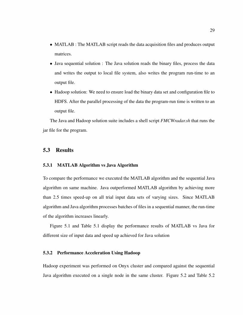
5.3.1 MATLAB Algorithm vs Java Algorithm . . . . . . . . . . . . . . . . . . . . . 29

5.3.2 Performance Acceleration Using Hadoop . . . . . . . . . . . . . . . . . . . . 29

5.4 Deploying Hadoop Solution on HPC Batch Systems . . . . . . . . . . . . . . . . . . 33

5.4.1 Running Hadoop Solution on Kestrel . . . . . . . . . . . . . . . . . . . . . . . 33

5.4.2 Results . . . . . . . . . . . . . . . . . . . . . . . . . . . . . . . . . . . . . . . . . . . . . . 34

5.4.3 Analysis . . . . . . . . . . . . . . . . . . . . . . . . . . . . . . . . . . . . . . . . . . . . . 35

6 Conclusion . . . . . . . . . . . . . . . . . . . . . . . . . . . . . . . . . . . . . . . . . . . . . . . . . . . . . 36

6.1 Summary . . . . . . . . . . . . . . . . . . . . . . . . . . . . . . . . . . . . . . . . . . . . . . . . . . 36

6.2 Results and Implications . . . . . . . . . . . . . . . . . . . . . . . . . . . . . . . . . . . . . . . 37

viii

6.3 Future Directions . . . . . . . . . . . . . . . . . . . . . . . . . . . . . . . . . . . . . . . . . . . . 38

REFERENCES . . . . . . . . . . . . . . . . . . . . . . . . . . . . . . . . . . . . . . . . . . . . . . . . . . . . 39

A Cluster Configuration . . . . . . . . . . . . . . . . . . . . . . . . . . . . . . . . . . . . . . . . . . . . 40

A.1 Onyx Cluster Configuration . . . . . . . . . . . . . . . . . . . . . . . . . . . . . . . . . . . . 40

A.2 Kestrel Configuration . . . . . . . . . . . . . . . . . . . . . . . . . . . . . . . . . . . . . . . . . 41

B Kestrel Scripts . . . . . . . . . . . . . . . . . . . . . . . . . . . . . . . . . . . . . . . . . . . . . . . . . . 42

B.1 PBS Job Script . . . . . . . . . . . . . . . . . . . . . . . . . . . . . . . . . . . . . . . . . . . . . . 42

B.2 Hadoop creation script . . . . . . . . . . . . . . . . . . . . . . . . . . . . . . . . . . . . . . . . 44

B.3 Cluster removal script . . . . . . . . . . . . . . . . . . . . . . . . . . . . . . . . . . . . . . . . . 45

ix

LIST OF TABLES

5.1 Run-time (seconds) performance of MATLAB and Java . . . . . . . . . . . . . . . 30

5.2 Run-time (seconds) performance on onyx machines for Java sequential,

Hadoop (distributed with 4 nodes), Hadoop (distributed with 8 nodes) . . . . 31

5.3 Speed up for Hadoop (distributed with 4 nodes), Hadoop (distributed with

8 nodes) compared with Java sequential solution . . . . . . . . . . . . . . . . . . . . 32

5.4 Run-time (seconds) performance of Hadoop on Kestrel Cluster . . . . . . . . . 35

A.1 Kestrel Node configuration . . . . . . . . . . . . . . . . . . . . . . . . . . . . . . . . . . . . 41

x

LIST OF FIGURES

2.1 Frequency vs time of FMCW radar . . . . . . . . . . . . . . . . . . . . . . . . . . . . . . . 6

2.2 Snow depth estimation results using FMCW radar . . . . . . . . . . . . . . . . . . . 7

2.3 Hadoop architecture . . . . . . . . . . . . . . . . . . . . . . . . . . . . . . . . . . . . . . . . . . 10

2.4 Mapreduce Model . . . . . . . . . . . . . . . . . . . . . . . . . . . . . . . . . . . . . . . . . . . 11

4.1 Conversion of input data format . . . . . . . . . . . . . . . . . . . . . . . . . . . . . . . . . 18

4.2 Stage 1 mapper and reducer . . . . . . . . . . . . . . . . . . . . . . . . . . . . . . . . . . . . 21

4.3 Stage 2 mapper . . . . . . . . . . . . . . . . . . . . . . . . . . . . . . . . . . . . . . . . . . . . . . 24

5.1 Run-time (seconds) performance of MATLAB and Java as graph . . . . . . . . 30

5.2 Run-time (seconds) performance of Java and Hadoop . . . . . . . . . . . . . . . . . 31

5.3 Run-time (seconds) performance of Hadoop algorithm on a 4 node cluster

with varying number of map tasks per node . . . . . . . . . . . . . . . . . . . . . . . . 32

5.4 Deploying Hadoop on Kestrel HPC . . . . . . . . . . . . . . . . . . . . . . . . . . . . . . 34

5.5 Runtime performance comparison for Onyx and Kestrel Hadoop clusters . . 35

A.1 Boise State University, Department of Computer Science, Onyx Cluster Lab 40

xi

LIST OF ABBREVIATIONS

SWE – Snow Water Equivalent

FMCW Radar – Frequency Modulated Continuous Wave Radar

DAQ files – Data Acquistion files

FFT – Fast Fourier Transform

HDFS – Hadoop Distributed File System

PSD – Power Spectral Density

GPU – Graphical Processing Unit

HPC – High Performance Cluster

xii

1

Chapter 1

INTRODUCTION

1.1 Overview

Geophysics is a field that integrates geology, mathematics, physics, engineering and com-

puter science in order to understand large scale subsurface earth processes. Geophysicists

study earth processes through a combination of field and laboratory experiments, compu-

tational and theoretical modeling, remote sensing, and direct in-site observation. Remote

sensing makes it possible to collect data at large scales on high temporal frequency, and

in dangerous or inaccessible areas of the earth using instruments on aircraft and satellites.

Researchers use the sensor data to answer scientific questions, develop models and make

predictions. Thus correct interpretation of data and the variables controlling uncertainties

are essential for obtaining accurate estimates.

The Cryosphere is the collection of places on earth where water is in solid form (e.g. ice

or snow). Snow cover in the cryosphere plays an important role in earth’s hydrologic cycle.

This forms a critical part of many northern ecosystems and provides irrigation for crops and

drinking water for communities. Remote sensing of snow helps in predicting the volume of

fresh water that a given snow-covered area represents, referred to as Snow Water Equivalent

(SWE), for water resource management, hydro-power, and flood forecasting. This predic-

tion process involves analysis of data acquired from sensors, such as radars, that monitor

the state of glaciers, polar ice caps, snowfall, oceans, and lakes in the Arctic, Antarctic,

2

and many mountainous regions of the world. Accurate estimates of SWE are becoming

more important as the distribution of snow is sensitive to climate change and expected

to change in future. Environmental factors like changes in temperature and precipitation

alter the distribution of snow, thereby making the prediction of water resources difficult.

Scientists compare several state-of-the-art methods for estimating SWE over large areas

by employing tools and techniques based on subsurface imaging, remote sensing, in-site

measurements, and modeling.

Frequency Modulated Continuous Wave (FMCW) [7] radar is an effective snow science

tool that has been successfully used by snow scientists around the world for studying snow

pack properties. FMCW radar is used to map snow depth, SWE, and snow stratigraphy.

To estimate snow properties, the raw data from FMCW radars needs to be processed with

frequency domain techniques and filtered to remove noise and incorrect readings before

any analysis is performed. After pre-processing, the results obtained need to be examined

by an experienced radar analyst to identify signals of interest, such as reflections from snow

layers. The rapid increase in the size of data recorded by the sensors is causing the steps of

pre-processing and finding results to be slow. When the results don’t reveal anything new

or if the prediction becomes inaccurate, the processed data is discarded. Experiments with

new signal processing techniques becomes difficult due to the computational time required

for these large datasets.

In this research, we implement a parallel processing algorithm using Hadoop to inves-

tigate the accelerated performance of the algorithm for snow depth estimation compared to

the single processor MATLAB solution currently used.

3

1.2 Outline

In Chapter 2, we provide a brief introduction on remote sensing of snow and background

theory on FMCW radar. We discuss the challenges faced by the current implementation and

possible solutions. We introduce the concept of Big Data, and provide relevant information

regarding the Hadoop framework considered in this research.

In Chapter 3, we introduce the snow research conducted by the CryoGARS [12] group

in Geosciences Department at Boise State University. We explain the algorithm used for

the snow depth estimation. In doing so, we formally present the problem statement that

was addressed in this project.

In Chapter 4, we present the design and implementation for the Java and Hadoop solu-

tions. First, we discuss the conversion of the existing MATLAB algorithm to Java. Then

we provide a summarized description of the algorithms used in the Hadoop MapReduce

solution.

In Chapter 5, we present the Hadoop performance comparison experiment. First, we

discuss the software and hardware environment in which our comparative benchmark anal-

ysis is conducted. Second, we provide the procedure used to guide and execute the ex-

periment. Finally, we present the performance results for the various experimental trial

runs. We also discuss the challenges faced in deploying the Hadoop solution on a High

Performance Computing (HPC) cluster using traditional batch job submission.

In Chapter 6, we conclude our report and suggest some future directions.

4

Chapter 2

BACKGROUND

2.1 Remote Sensing of Snow

Snow on the earth’s surface is an accumulation of ice crystals or grains, resulting in a

snowpack which over an area may cover the ground either partially or completely. Remote

sensing of snow offers a new and valuable tool for estimating snow properties. This helps

scientists to estimate the amount of water stored in the seasonal snow cover. Remote

sensing is performed with optical, microwave and gravity sensors from ground based,

air borne and satellite platforms. Microwave radar is a promising technique for remote

sensing because it can penetrate snow, providing information on the snowpack properties

like snow depth, SWE and the presence of liquid water in the snowpack, which is of most

interest to hydrologists. Optical sensors can only give information about the snow covered

area and snow surface properties while microwave radar is required for subsurface snow

information.

2.2 FMCW Radar

Frequency Modulated Continuous Wave (FMCW) [9] radar is a popular snow science tool

for monitoring avalanche flow, measuring stratigraphy, snow depth, and SWE, as well

as for ground truth of remote sensing. FMCW radar is used for making high resolution

5

measurements of snow structure over large distances, as well as continuous measurements

throughout the winter. Microwave radiation emitted from the radar in a snow covered

area gets reflected back from the snow surface, snow layers and the underlying ground

and is scattered in many different directions by the snow grains within each snow layer.

Active microwave radar backscatter increases with increase in snow and the travel time

of the microwave signals through snow can be used to estimate snow depth and SWE. The

sensitivity of the microwave radiation to snow on the ground makes it also possible to mon-

itor snow cover using passive microwave remote sensing techniques to derive information

on snow extent, snow depth, snow water equivalent and snow state. Properties affecting

microwave response from a snowpack include depth and water equivalent, liquid water

content, density, grain size and shape, temperature and stratification as well as snow state

and land cover.

The raw data acquired from ground based FMCW radar can be processed and inter-

preted to estimate snow depth, SWE, snow stratigraphy in wet and dry snow conditions.

This helps scientists get better understanding of the spatial and temporal variability of snow

structure and its effect on remote-sensing measurements [5].

2.2.1 FMCW Radar Explained

FMCW radar is used to measure the travel time of the transmitted microwave signal through

the underlying snow pack. This transit time is proportional to the electrical depth of the

snow.

The radar technique uses a voltage-controlled oscillator to transmit a continuous sinu-

soidal electromagnetic wave, whose frequency varies linearly with time over a wide band-

width. The transmitted wave spans a length of time which is several orders of magnitude

larger than the two-way travel time to reflectors of interest. A portion of the transmitted

6

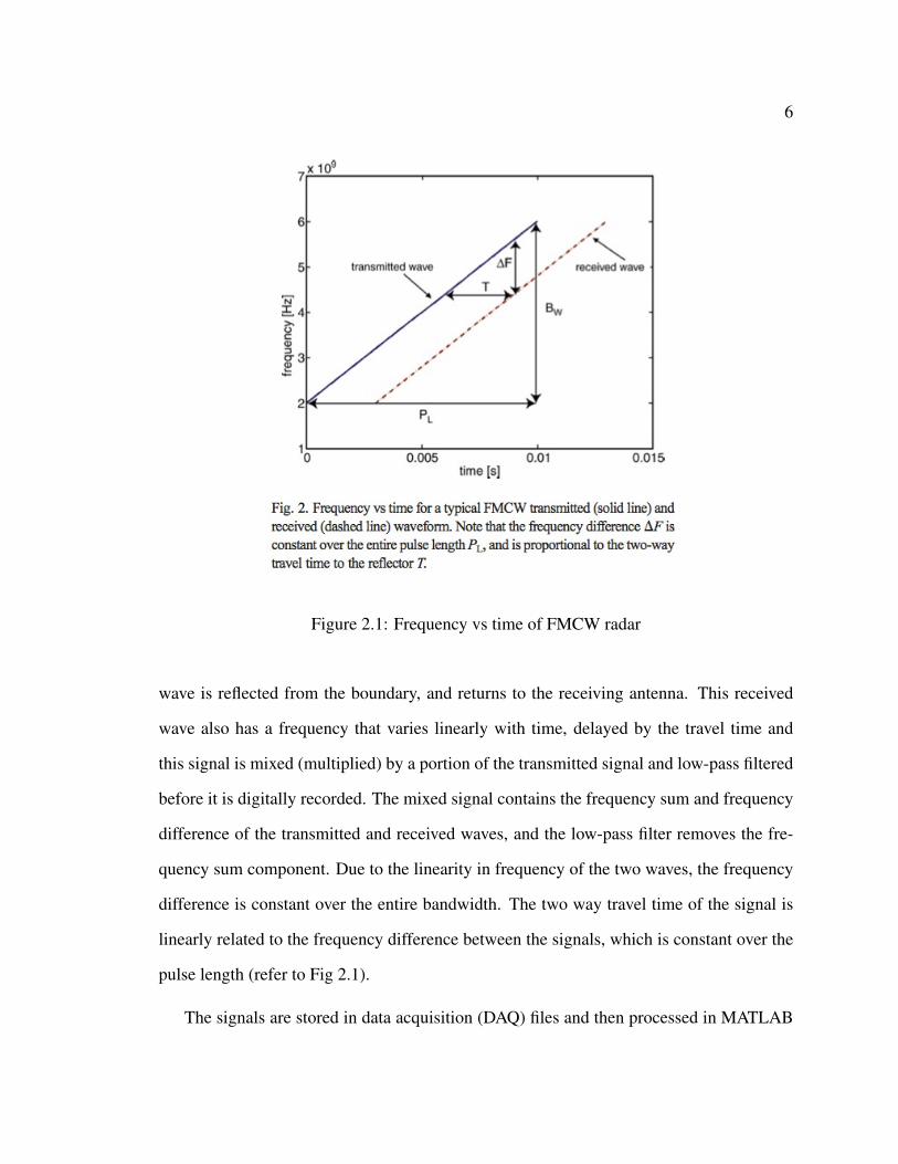
Figure 2.1: Frequency vs time of FMCW radar

wave is reflected from the boundary, and returns to the receiving antenna. This received

wave also has a frequency that varies linearly with time, delayed by the travel time and

this signal is mixed (multiplied) by a portion of the transmitted signal and low-pass filtered

before it is digitally recorded. The mixed signal contains the frequency sum and frequency

difference of the transmitted and received waves, and the low-pass filter removes the fre-

quency sum component. Due to the linearity in frequency of the two waves, the frequency

difference is constant over the entire bandwidth. The two way travel time of the signal is

linearly related to the frequency difference between the signals, which is constant over the

pulse length (refer to Fig 2.1).

The signals are stored in data acquisition (DAQ) files and then processed in MATLAB

7

Figure 2.2: Snow depth estimation results using FMCW radar

using one or more CPUs or GPUs. The signals from the files are first subdivided over the

frequencies of interest, followed by a windowed Fast-Fourier Transform (FFT) operation

to transform them from time domain into the frequency domain, where the frequency

difference can be used to measure the two-way travel time and the electrical distance to

a given reflector [9]. Fig 2.1 shows the frequency of both the transmitted and received

waves as a function of time. The constant frequency difference between transmitted and

received signals of an FMCW radar is proportional to the signal travel time to the reflector,

and the distance to the reflector can be calculated using the bandwidth, pulse length and

velocity of the signal. Depth of snow can be found by solving for the electrical depth of

snow and a rough estimate of snow density to determine the velocity. SWE estimates from

this method are less sensitive to density changes than depth estimates.

The above mentioned calculations can be generalized to the case of multiple reflectors

and the result obtained is a radar image that contains peaks in amplitude from major re-

8

flectors in the snowpack (surface, snow layers, ground). Fig 2.2 shows results of processed

signals from a portable FMCW radar in Devon Ice Cap, Nunavut, Canada [8]. The image

shows strong layer reflections occurred down to approximately 2 m, and the thickness

of layers could be used to infer annual accumulation rates. The current software used for

signal analysis can process a sample lasting 600 seconds and calculate the major reflections

in around 90 seconds of computation.

More and more data is collected every year from different parts of the world under

various conditions in an effort to understand snow distribution and variability. The increase

in size of the input data slows down the speed of processing algorithm as it involves steps

like FFTs and convolutions that are heavily CPU-bound [1] and the results obtained are

not always accurate. This restricts the researchers from making use of all the data being

collected to come up with an accurate model. Another side effect of the pre-processing step

is the storage requirement for the processed data. A sample data set of 2GB of input files

produces 20GB of processed data as output. This strongly implies the need for increased

storage space and high processing power to deal with the huge amounts of data.

2.3 Parallel Processing and Big Data

The snow depth estimation algorithm is currently implemented in MATLAB [10]. MAT-

LAB provides an effective numerical computing environment and programming platform

for geoscientists to perform matrix operations, fit surfaces to the data, perform regressions,

plot maps, and find correlations very easily. It has elegant matrix support and visualization.

But solving technical computing problems that require processing and analyzing large

amounts of data puts a high demand on the amount of memory required. Large data

sets take up significant memory during processing and can require many operations to

9

compute a solution. It can also take a long time to access information from large set of

data files. MATLAB is not open source and hence cannot be installed in every machine to

process the data in a distributed fashion without large cost. Another drawback is the lack of

scalability as the number of input data files expands. The snow depth estimation algorithm

also contains methods that are inherently parallel making them well suited for processing

in a parallel computing environment.

2.3.1 Hadoop Distributed Filesystem

Hadoop is an open-source implementation of the MapReduce framework developed by

Google. The Apache Software Foundation and Yahoo! released the first version in 2004

and continues to extend the framework with new sub-projects. Hadoop provides several

open-source projects for reliable, scalable, and distributed computing [4]. This project uses

the Hadoop Distributed Filesystem (HDFS) [6] and Hadoop MapReduce [3].

HDFS is a scalable distributed filesystem that provides high-throughput access to ap-

plication data [6]. A HDFS cluster consists of one master as namenode and a number of

cluster nodes as datanodes. The namenode is responsible for managing the filesystem tree,

the metadata for all the files and directories stored in the tree, and the locations of all blocks

stored on the datanodes. Datanodes are responsible for storing and retrieving blocks when

the namenode or clients request them.

2.3.2 MapReduce

MapReduce is a programming model on top of HDFS for processing and generating large

data sets that was developed as an abstraction of the map and reduce primitives present

in many functional languages [3]. The abstraction of parallelization, fault tolerance, data

distribution and load balancing allows users to parallelize large computations easily. The

10

Figure 2.3: Hadoop architecture

MapReduce model works well for Big Data analysis because it is inherently parallel and

can easily handle data sets spanning across multiple machines.

As volume of data grows rapidly, Hadoop MapReduce provides an efficient processing

framework, required to process massive amount of data in parallel on large clusters.

Each MapReduce program runs in two main phases: the map phase followed by the

reduce phase. The programmer simply defines the functions for each phase and Hadoop

handles the data aggregation, sorting, and message passing between nodes. There can be

multiple map and reduce phases in a single data analysis program with possible dependen-

cies between them.

Map Phase. The input to the map phase is the raw data. A map function should prepare

the data for input to the reducer by mapping the key to the the value for each “line”

of input. The key-value pairs output by the map function are sorted and grouped by

key before being sent to the reduce phase.

11

Figure 2.4: Mapreduce Model

Reduce Phase. The input to the reduce phase is the output from the map phase, where the

value is an iterable list of the values with matching keys. The reduce function should

iterate through the list and perform some operation on the data before outputting the

final result.

The steps involved in working of Hadoop MapReduce includes job submission, job

initialization, task assignment, task execution, program and status updates, and job com-

pletion. A Job is used to describe all inputs, outputs, classes, and libraries used in a

MapReduce program, whereas a program that executes individual map and reduce steps

is called as a task. When a job is submitted, JobTracker schedules the jobs on TaskTracker

nodes, monitors them, reexecutes them in case of failure and synchronizes them. The

datanodes are the cluster nodes that runs the TaskTracker to execute the tasks chosen by

JobTracker. The Hadoop application uses HDFS as a primary storage to construct multiple

replicas of data blocks and distributes them on the cluster nodes. Input and output files

12

for Hadoop programs are stored in HDFS, which provides high input and output speeds by

storing portions of files scattered throughout the Hadoop cluster.

13

Chapter 3

SIGNAL PROCESSING AND PROBLEM STATEMENT

The CryoSphere Geophysics and Remote Sensing (CryoGARS) [12] group, within the Geo-

sciences Department at Boise State University, focuses on answering scientific questions

about the snow and ice covered areas of the world (the Cryosphere) using state of the art

geophysical, remote sensing, modeling and engineering methods. The current research of

the group includes quantifying the spatial variability of snow properties using ground-based

microwave radar and snow micropenetrometry, improving estimates of snow properties

from airborne and satellite-based radar, detection of oil spills under sea ice with radar,

quantifying lateral flow of water within the snowpack, and detection of avalanches with

infrasonics.

Research on snow depth estimation by the CryoGARS group uses FMCW radar technol-

ogy. The advanced FMCW radars provide snow scientists and hydrologists with the ability

to map snow pack properties, such as depth, SWE and stratigraphy, rapidly over large

distances, at high resolution. The scientists use processing algorithms to identify previously

unrecognized patterns and trends hidden within the vast amounts of data available to them.

The processing algorithm requires scientists to manually choose the processing parameters.

This is a tedious effort and the parameters might not always be optimal. The results

obtained after the long processing steps need careful examination where scientists look

for patterns in the signal characteristics and determine the resolution of measurements of

14

snow structure and make predictions. This step also takes into consideration the hetero-

geneous properties of snow, which significantly affects the accuracy of predictions. If the

predictions turn out to be inaccurate, the processing step is repeated with a different set

of parameters until an accurate prediction is made. The speed of the processing algorithm

becomes critical as this is a repetitive process until they derive an accurate model from the

data.

3.1 Snow Depth Estimation Algorithm

The algorithm for snow depth estimation is divided into two main steps,

1. Subdividing: This is the first step that reads the raw radar sensor data files with

continuous ramp of voltage signals and subdivides to output a smoothed time domain

matrix data based on the value of all the processing parameters.

2. Power Spectral Density estimation: The second step involves converting the time

domain data to frequency domain data using a windowed FFT and then calculating

the power spectral density.

The input files are in Data acquisition format (.daq extension), which is a MATLAB

proprietary format. Each file is read to form a time domain matrix. The files are grouped

into batches and the matrix for each file is combined to form the time domain matrix for the

whole batch. Later the time domain matrix for each batch is converted to frequency domain

matrix by applying FFT on the time domain matrix and the output is used to calculate the

power spectral density matrix. The power spectral density matrix is used get a radar image

showing the snow depth estimates for a given area.

The above mentioned two steps are performed on every batch iteratively and are iden-

tified as steps that can be performed in parallel.

15

3.2 Problem Statement

The research group has over 6TB of radar data for snow research collected over years

from different locations and testing conditions. The amount of data generated is increasing

exponentially as more observations are being captured to improve the models and snow

depth estimation to enable better predictions. The speed of the processing algorithm does

not scale with the size of the input data, which limits the researchers from using all of the

data acquired for modeling.

Challenges faced :

1. There is too much data to store and process on single machine.

2. Use of expensive software.

3. The current algorithm process data files as sequential batches, which requires a lot of

processing time.

4. Algorithm uses CPU bound operations like FFT calculations.

5. Accelerated processing using GPUs are also reaching memory limits.

This project was an effort to find out if we can use a parallel model, such as MapReduce,

to accelerate the speed of the algorithm on big data sets by performing the repetitive steps

of the algorithm in parallel.

Thus, the goals of the project were:

• Convert the existing MATLAB algorithm to Java.

• Compare the performance of MATLAB and Java implementation on a sample data

set.

• Implement Hadoop MapReduce solution.

• Compare the speed of Hadoop and sequential Java algorithms on a sample data set.

• Compare the correctness of the output from Hadoop.

16

• Test the Hadoop algorithm on larger datasets.

• Compare the algorithm run-time of MATLAB, Java and Hadoop solutions.

• Deploy the Hadoop solution on HPC using traditional batch jobs.

The data points collected from the above experiments will help answering the following

questions.

1. How much performance gain can be achieved by using Java and Hadoop solutions?

2. How much cost and effort will it take to deploy Hadoop solution?

17

Chapter 4

DESIGN AND IMPLEMENTATION

The process for the design and implementation of Hadoop solutions for snow depth estima-

tion is carried out in two distinct phases: Conversion to Java and Hadoop implementation.

4.1 Conversion to Java

As a first step of the speed improvement, the MATLAB algorithm is converted to Java.

Java’s write once, run anywhere is a key aspect in considering it as a choice of language for

conversion. It is dynamic, extensible and modular with object oriented features. Converting

the algorithm to Java also enables easy porting to Hadoop due its inherent Java support.

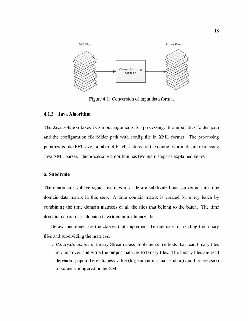
4.1.1 Data Format Conversion

The MATLAB reads the radar data acquisition files using daqread function and converts

the voltage signals recorded in them to matrices for further computations.

Since the ability to read .daq files directly from third-party software is not available,

they are converted to binary format that can be interpreted in Java. The binary files contain

the time information when the file was recorded followed by voltage signals values, all of

them being stored as single precision floating point numbers.

18

Figure 4.1: Conversion of input data format

4.1.2 Java Algorithm

The Java solution takes two input arguments for processing: the input files folder path

and the configuration file folder path with config file in XML format. The processing

parameters like FFT size, number of batches stored in the configuration file are read using

Java XML parser. The processing algorithm has two main steps as explained below:

a. Subdivide

The continuous voltage signal readings in a file are subdivided and converted into time

domain data matrix in this step. A time domain matrix is created for every batch by

combining the time domain matrices of all the files that belong to the batch. The time

domain matrix for each batch is written into a binary file.

Below mentioned are the classes that implement the methods for reading the binary

files and subdividing the matrices.

1. BinaryStream.java: Binary Stream class implements methods that read binary files

into matrices and write the output matrices to binary files. The binary files are read

depending upon the endianess value (big endian or small endian) and the precision

of values configured in the XML.

19

public double [][] byteToMatrix(byte[] binaryData ,int row , int

column)

public byte[] matrixToBytes(double [][] matrix)

public byte[] arrayToBytes(double [] matrix)

static double [] byteToArray(byte[] byteArray)

public double getCpuInfo(byte[] bytesValue)

2. SubdivideDAQ.java :

This class implements the subdividing function. The input binary file is converted

into a matrix and subdivided and returns a time domain matrix as output. The main

methods implemented in this class are:

private double [][] findTrace ()

private double [][] subDivideDAQ ()

3. ConfigSettings.java : This class has methods to parse the XML file with configuration

parameters using built-in Java XML parser class. Method implemented here is:

public void readXML(FSDataInputStream fis)

b. Power Spectral Density Estimation

This step reads time domain data matrix output files from Step 1 and converts to frequency

domain using FFT. Before an FFT operation, the time domain matrix is prepared with

Kaiser Bessel Window using modified Bessel function of the first kind.

The Kaiser Bessel function is implemented with the help of an open source Java library

[5]. Then FFT is computed using open source library JTransforms [13] where the size of

the FFT is determined from configuration file. The output of FFT is then used to calculate

the power spectral density estimate. Following classes implement this step:

1. CalculatePSDRadar.java: This class contains methods to calculate the Kaiser Bessel

window, prepare the time domain matrix using Kaiser Bessel window, compute the

FFT and calculate the power spectral density matrix from the FFT output. The main

methods in this class are :

public static double [] KaiserBessel(int N, double alpha , int

nfft)

20

public static double [][] prepareMatrix(double [] kbWindow ,

double [][] TDATA)

public static double [][] performFFT(double [][] TDATA , int

nfft ,int tdataColumns)

public static double [][] estimatePSD(double [][] D, double [] wj)

4.1.3 Output Files

The output files are stored in binary format. The files contain matrices for time domain

data, frequency domain data, CPU time information matrix and the file number array for

each batch. These can be loaded into MATLAB to plot the radar image for predicting the

snow depth.

4.2 Hadoop Solution

The Hadoop MapReduce solution is implemented as two map-reduce job phases that are

detailed in the following sections. The output time domain data from the first job serves as

the input to the second job and the final results are stored in HDFS. The first job takes the

input files folder and the configuration file folder paths as input.

4.2.1 Stage 1: Subdividing

The first stage of the Hadoop implementation subdivides the voltage signals recorded in the

input binary files to obtain the time domain data matrix. Figure 4.2 provides an overview

of the Stage 1 described below.

The first stage mapper reads the input binary files using CombineFileInputFormat. The

size of each input binary file is very small when compared to the default block size of

hadoop (64MB). Map tasks usually process a block of input at a time using the default

FileInputFormat. When the input file is very small and the data set is large, then each map

21

Figure 4.2: Stage 1 mapper and reducer

task processes very little input. Since there are numerous map tasks in this case, extra

overhead caused by managing these tasks results in job time becoming tens or hundreds of

times slower than the equivalent one with a large single input file. This problem is solved

by using CombineFileInputFormat.

22

CombineFileInputFormat helps in processing large number of small files. As given in

the description of the class, splits are constructed from the files under the input paths. Each

split returned may contain blocks from different files. If a maxSplitSize is specified, then

blocks on the same node are combined to form a single split. Blocks that are left over are

then combined with other blocks in the same rack. If the maxSplitSize is equal to the

block size, then this class is similar to the default splitting behavior in Hadoop: each block

is a locally processed split. This is implemented using three classes, WholeFileInputFor-

mat, WholeFileRecordReader and FileNameWritable.

WholeFileInputFormat is a subclass of CombineFileInputFormat. This subclass will

initiate a delegate WholeFileRecordReader that extends RecordReader. The chunk size is

controlled by calling the setMaxSplitSize method. As we need to read each file as whole

record, isSplitable method is set to return false which defaults to true.

WholeFileRecordReader is a class that passes each split (typically a whole file) to class

WholeFileInputFormat. When the Hadoop job starts, WholeFileRecordReader reads all

the file sizes in HDFS that we want to process, and decides how many splits based on

the MaxSplitSize we defined in WholeFileInputFormat. For every split that is a file (file

isSplitable is set as false) CombineFileRecordReader creates a WholeFileRecordReader

instance via a custom constructor, and passes in CombineFileSplit, context, and index for

WholeRecordReader to locate the file to process with.

When processing the file, the WholeFileRecordReader creates a FileNameWritable as

the custom key for Hadoop mapper class. FileNameWritable consists of file name and the

offset length of that line. The difference between FileNameWritable and the normally used

LongWritable in mapper is that LongWritable only denotes the offset of a line in a file,

while FileNameWritable adds the file information into the key.

The input key for mapper is the FileNameWritable that provides the file name and

23

input value is the BytesWritable value that is the content of the file. The output key of

the mapper is batch number, which the file belongs to as a Text value, and output value is

a comma-seperated Text values with time domain data matrix index offset and the matrix

value for that index.

The code below shows the mapper class for Stage 1 that mainly performs the subdivid-

ing functions:

public static class job1Map extends Mapper <FileNameWritable ,

BytesWritable , Text , Text >

{

SubDivideDAQ subdivideObj = new

SubDivideDAQ(fileMatrix ,cpuTimeFromFile);

double [][] TDATA = subdivideObj.getTDATA(processing params);

}

At Stage 1 reducer, all the data values for a batch comes under the same reducer. The

time domain data matrix for every batch is constructed from each key-value pair. Each

item in the value list for a batch is a pair of comma-separated values for index offset and

matrix value. The time domain data matrix thus obtained is the output for job 1 and is

written to HDFS. The matrix is converted to BytesWritable format and MultipleOutputs

class simplifies writing output data to multiple outputs files.

public static class job1Reduce extends Reducer <Text , Text ,

NullWritable , BytesWritable >

{

MultipleOutputs mos = new MultipleOutputs <NullWritable ,

BytesWritable >( context);

BytesWritable outputValue = new

BytesWritable(bs.matrixToBytes(wholeTDATA));

mos.write( NullWritable.get(), outputValue ,

"tdatasamples/"+key.toString ());

}

4.2.2 Stage 2: Power Spectral Density Calculations

The second stage requires the output of Stage 1, the time domain data matrices that are

stored in binary form. This stage has only mapper process and uses WholeFileInputFormat

24

for InputFormat class.

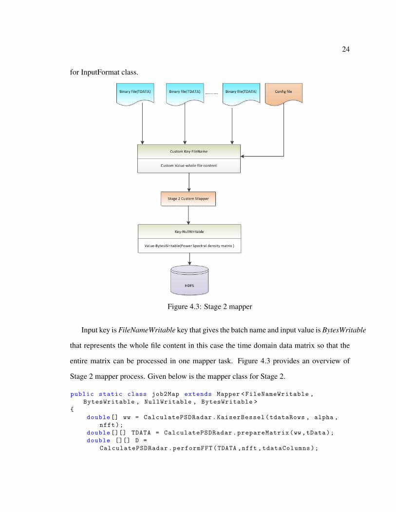
Figure 4.3: Stage 2 mapper

Input key is FileNameWritable key that gives the batch name and input value is BytesWritable

that represents the whole file content in this case the time domain data matrix so that the

entire matrix can be processed in one mapper task. Figure 4.3 provides an overview of

Stage 2 mapper process. Given below is the mapper class for Stage 2.

public static class job2Map extends Mapper <FileNameWritable ,

BytesWritable , NullWritable , BytesWritable >

{

double [] ww = CalculatePSDRadar.KaiserBessel(tdataRows , alpha ,

nfft);

double [][] TDATA = CalculatePSDRadar.prepareMatrix(ww ,tData);

double [][] D =

CalculatePSDRadar.performFFT(TDATA ,nfft ,tdataColumns);

25

double [][] P = CalculatePSDRadar.estimatePSD(D, ww);

mos.write( NullWritable.get(), outputValue ,

"pdatasamples/"+key.toString ());

}

The output of the mapper is the final result and this step doesn’t have any reducers. The

power density spectral data matrices calculated in the mapper for each batch is written in a

file in double precision binary values. These binary files can be later loaded in MATLAB

and can be plotted into diagrams to estimate the snow depth.

4.2.3 Validation

The results of the Java and Hadoop programs were validated against the MATLAB output

files using a test program developed in Java. This program compares the binary result files

from MATLAB and Java solutions to find the deviation of the output values by checking the

relative error. The idea of a relative comparison is to find the difference between the actual

and expected numbers and see how big it is compared to their magnitudes. A maximum

relative error value of 0.00001 is specified in the program to denote the maximum relative

error we can tolerate. In order to get correct results, the relative error of two values is

always compared to the larger value among actual and expected value.

It has been observed that all the values in the time domain data matrix output of Java so-

lution exhibited no difference when compared with the MATLAB output denoting that the

output values were same. While validating power spectral density output, the comparison

exhibited small relative error. None of the values had relative error greater than 0.00001.

This shows 99.999 percent accuracy of the Java output compared to MATLAB solution.

The small relative error occurred in the comparison may be attributed to limited floating

point precision. The differences in rounding methodologies in floating point computations

of different open source libraries may also contribute to this variance. The results of

26

validation shows that output obtained from Java algorithm is same as the output computed

in MATLAB, thereby making Java solution adequate for snow depth estimation.

27

Chapter 5

EXPERIMENTAL RESULTS AND ANALYSIS

This chapter describes the MATLAB, Java and Hadoop performance comparison exper-

iment for snow depth estimation algorithm. The goal was to study and prove that Java

and Hadoop solutions provides faster processing of radar data than existing MATLAB

implementation.

The experiments for comparison of MATLAB and sequential Java algorithm were per-

formed in Boise State University machine, mec302rcuda, a departmental workstation. This

machine is an Intel(R) Core(TM) i7 CPU 930 @ 2.80GHz processor with 4 hyper-threaded

cores.

The Hadoop experiment was conducted on the Onyx cluster and Kestrel cluster at

Boise State University. The cluster configuration and detailed hardware specifications are

provided in Appendix A. Before each execution, we ensured that all nodes were alive and

that the integrity of the data was unaltered. The sequential Java program was executed on

a single node in the appropriate cluster to compare the performance.

5.1 Setup

5.1.1 MATLAB and Sequential Java

The comparison was performed by running MATLAB and Java programs in a machine

in Boise State University Computer Science department. The MATLAB version used in

28

this experiment is Release 2013a. The algorithm was executed with a MATLAB script

that reads the input DAQ files from the folder specified in the script. The sequential Java

program was run using Java 1.8.0 05 version. The Java programs were compiled and built

using Apache Maven [11].

5.1.2 Hadoop

For the parallel computing experiment, Hadoop version 1.2.1 was used along with Java

version 1.8.0 05 in Onyx cluster. We configured the HDFS namenode and MapReduce

JobTracker on the Onyx masternode along with 8 compute nodes as HDFS datanodes and

MapReduce TaskTrackers. The experiment was also repeated with 4 compute nodes for the

same data sets. Note that since the purpose of the namenode is to maintain the filesystem

tree, the metadata for directories in the tree, and the datanode on which all the blocks for a

given file are located, it does not add computing power for MapReduce in this experiment.

The maximum number of map and reduce tasks were set to 16 and 17, respectively. We

left the default replication factor of 3 per block, without compression. Data for both the

namenode and datanodes are stored on an ext4 directory of the local filesystem. Java heap

space for the Hadoop job was set to 2 GB in mapred-site.xml Hadoop configuration file

as the tasks in the job are compute intensive.

5.2 Execution

To determine how much the Java and Hadoop solutions outperformed MATLAB, we exe-

cuted the programs on a sample 2GB data set. The batch size was given the value 50 in the

configuration file.

29

• MATLAB : The MATLAB script reads the data acquisition files and produces output

matrices.

• Java sequential solution : The Java solution reads the binary files, process the data

and writes the output to local file system, also writes the program run-time to an

output file.

• Hadoop solution: We need to ensure load the binary data set and configuration file to

HDFS. After the parallel processing of the data the program-run time is written to an

output file.

The Java and Hadoop solution suite includes a shell script FMCWradar.sh that runs the

jar file for the program.

5.3 Results

5.3.1 MATLAB Algorithm vs Java Algorithm

To compare the performance we executed the MATLAB algorithm and the sequential Java

algorithm on same machine. Java outperformed MATLAB algorithm by achieving more

than 2.5 times speed-up on all trial input data sets of varying sizes. Since MATLAB

algorithm and Java algorithm processes batches of files in a sequential manner, the run-time

of the algorithm increases linearly.

Figure 5.1 and Table 5.1 display the performance results of MATLAB vs Java for

different size of input data and speed up achieved for Java solution

5.3.2 Performance Acceleration Using Hadoop

Hadoop experiment was performed on Onyx cluster and compared against the sequential

Java algorithm executed on a single node in the same cluster. Figure 5.2 and Table 5.2

30

Table 5.1: Run-time (seconds) performance of MATLAB and Java

# Size of data in GB MATLAB Java Speed-up for Java (x times)

0.5 415 162 2.51 830 324 2.62 1689 660 2.54 3301 1299 2.5

Figure 5.1: Run-time (seconds) performance of MATLAB and Java as graph

display the performance for Hadoop MapReduce and Java sequential algorithm for each

trial size.

It is evident from the results that Hadoop outperforms sequential Java program and

MATLAB on all of the sample data set sizes used in this experiment by a dramatic margin.

It was observed that Hadoop solution, for both 4 node and 8 node cluster configuration, is

significantly faster than its sequential Java counterpart.

Table 5.3 shows the speedup for Hadoop programs when compared with Java sequential

solution. The 4 node configuration is 1.3 - 2 times faster and the 8 node configuration is 2

- 4 times faster depending the input data set size. Its worth noting that adding more nodes

31

Table 5.2: Run-time (seconds) performance on onyx machines for Java sequential, Hadoop(distributed with 4 nodes), Hadoop (distributed with 8 nodes)

# Size of data in GB Java Hadoop (4 node) Hadoop (8 node)

1 441 309 2212 832 624 3374 1664 849 422

Figure 5.2: Run-time (seconds) performance of Java and Hadoop

to cluster is meaningful only for large data set as we can see that the 4 node configuration

performed better than the 8 node cluster for 1GB data set while 8 node cluster performed

significantly faster for 4GB dataset. It can also be observed that 8 node configuration

continued to take lesser time as the data set size increased.

From the performance analysis of above experiments, Hadoop MapReduce emerges

as the best candidate solution for processing large radar signal datasets. Furthermore, we

investigate whether we can improve MapReduce performance by varying the number of

map tasks per datanode: Figure 5.3 displays the results for 1, 2, and 4 map tasks per

32

Table 5.3: Speed up for Hadoop (distributed with 4 nodes), Hadoop (distributed with 8nodes) compared with Java sequential solution

# Size of data (GB) Hadoop 4 node ( x times) Hadoop 8 node (x times)

1 1.42 22 1.33 2.54 1.95 3.95

datanode. In this case, we observe that MapReduce with 4 map task per datanode slightly

outperforms job with lesser map tasks per datanode.

Figure 5.3: Run-time (seconds) performance of Hadoop algorithm on a 4 node cluster withvarying number of map tasks per node

The same experiment was performed on an 8 node cluster by varying the number of

map tasks per datanode. The results turned out to show the same behavior as in a 4 node

cluster where job with 4 map task per data node performed better than 2 or 1 map tasks per

datanode.

33

5.4 Deploying Hadoop Solution on HPC Batch Systems

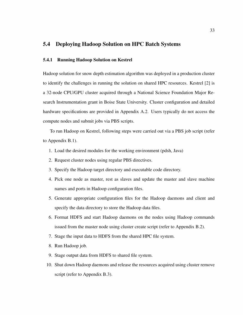
5.4.1 Running Hadoop Solution on Kestrel

Hadoop solution for snow depth estimation algorithm was deployed in a production cluster

to identify the challenges in running the solution on shared HPC resources. Kestrel [2] is

a 32-node CPU/GPU cluster acquired through a National Science Foundation Major Re-

search Instrumentation grant in Boise State University. Cluster configuration and detailed

hardware specifications are provided in Appendix A.2. Users typically do not access the

compute nodes and submit jobs via PBS scripts.

To run Hadoop on Kestrel, following steps were carried out via a PBS job script (refer

to Appendix B.1).

1. Load the desired modules for the working environment (pdsh, Java)

2. Request cluster nodes using regular PBS directives.

3. Specify the Hadoop target directory and executable code directory.

4. Pick one node as master, rest as slaves and update the master and slave machine

names and ports in Hadoop configuration files.

5. Generate appropriate configuration files for the Hadoop daemons and client and

specify the data directory to store the Hadoop data files.

6. Format HDFS and start Hadoop daemons on the nodes using Hadoop commands

issued from the master node using cluster create script (refer to Appendix B.2).

7. Stage the input data to HDFS from the shared HPC file system.

8. Run Hadoop job.

9. Stage output data from HDFS to shared file system.

10. Shut down Hadoop daemons and release the resources acquired using cluster remove

script (refer to Appendix B.3).

34

Figure 5.4: Deploying Hadoop on Kestrel HPC

5.4.2 Results

Hadoop experimental solution was successfully tested with input data sets of size ranging

from 1 GB to 4 GB on 4 and 8 nodes clusters. Java heap size for job was set to 2 GB and

output compression was enabled. The number of mapper tasks per node was set to 16 and

reducer tasks per node was set to 8.

Hadoop solution performance was compared against the sequential Java solution that

was executed in one of the Kestrel nodes. Table 5.4 shows the run time performance in

seconds in Kestrel for sequential Java, Hadoop on 4 node configuration and Hadoop on 8

node configuration. It was observed that Hadoop solution on 4 node cluster was 2.3 - 4.3

times faster and 8 node cluster was 2.6 - 6 times faster than the sequential Java solution

depending upon input data set size.

Performance of Hadoop on Kestrel and Hadoop on Onyx were also compared. Figure

35

Table 5.4: Run-time (seconds) performance of Hadoop on Kestrel Cluster

Size of data(GB) Sequential Java Hadoop (4 node) Hadoop (8 node)

1 315 135 1222 633 169 1464 1273 294 208

Figure 5.5: Runtime performance comparison for Onyx and Kestrel Hadoop clusters

5.5 shows the performance comparison and its evident that Kestrel outperforms Onyx in all

sample dataset sizes. Kestrel was 2.5 - 4 times faster than Onyx depending upon the input

dataset size and cluster size.

5.4.3 Analysis

The experiments prove that Hadoop solution can be successfully deployed in Kestrel using

PBS based job scheduler for large data sets. The performance analysis shows that running

the Hadoop solution on a high performance computing cluster can achieve significant speed

up in the processing time for large radar signal datasets. This also allows users to run

their pre-existing Hadoop jobs without needing a dedicated Hadoop cluster by leveraging

existing HPC resources.

36

Chapter 6

CONCLUSION

In this chapter we conclude by summarizing our findings and results on the parallel pro-

cessing of large radar data sets for snow depth estimation using Hadoop.

6.1 Summary

In Chapter 1, we introduced the concepts behind this project. We provided brief introduc-

tion of Geophysics and remote sensing. We stated why this is important for conducting this

research.

In Chapter 2, we provided background concepts for remote sensing and on the theory

of FMCW radar. We outlined some major challenges faced when processing large amounts

of data. We introduced the notion of Big Data and provided relevant information regarding

the Hadoop solutions considered in this research.

In Chapter 3, we introduced the snow depth detection algorithm and the steps involved.

We also discussed why a parallel solution is feasible for this algorithm. In doing so, we

formally presented the problem statement and the problems we wish to address in this

project.

In Chapter 4, we defined the design and implementation for the sequential and parallel

solutions using Java and Hadoop respectively. First, we discussed the conversion of the

37

MATLAB algorithm to Java. Second, we discussed Hadoop MapReduce implementation

and the details (as presented in Chapter 3).

In Chapter 5, we compared the results of MATLAB, Java and Hadoop algorithms. We

discussed the efficiency and scalability for these implementations alone with the resulting

implications and analysis. We also discussed the steps in deploying the Hadoop solution

in Kestrel and analyzed the challenges and performance in running the Hadoop solution in

HPC.

6.2 Results and Implications

From the performance comparison between MATLAB, Java and Hadoop experiments con-

ducted for this research, we conclude that:

1. Java sequential solution outperformed MATLAB for every data size.

2. Hadoop solution performs better than sequential Java implementation and the perfor-

mance advantage grows with increase of input data set size and cluster size.

3. Hadoop solution was successfully deployed in a HPC via traditional batch job sub-

mission and the results demonstrated improved performance compared to existing

solutions.

In addition to the performance advantages, having the knowledge base and source code

for Java/Hadoop implementation helps debugging and triaging the solutions to meet our

custom requirements easily. Thus Hadoop MapReduce turns out to be the best candidate

for processing large amounts of data collected by the radars for snow depth estimation

research.

38

6.3 Future Directions

Beyond the scope of this project, it would be interesting to investigate how much time and

effort will be required for further optimizing and improving the Hadoop implementation.

Additional research can be done to study the performance of Hadoop solution using large

data sets on clusters with more nodes, investigating the performance acceleration by fine

tuning Hadoop configurations and making use of GPU capabilities during parallel process-

ing. Future research can also involve implementing a runtime/state logging system to the

existing solution for effective and easy triaging.

39

REFERENCES

[1] G. D. Bergland. A guided tour of the fast fourier transform. IEEE Spectrum, 6(7):41–52, July 1969.

[2] Kestrel CPU/GPU cluster in Boise State University. http://wiki.boisestate.

edu/wiki/the-kestral-cpugpu-cluster/.

[3] Jeffrey Dean and Sanjay Ghemawat. Mapreduce: Simplified data processing on largeclusters. MapReduce: Simplified Data Processing on Large Clusters, December 2004.

[4] Apache Hadoop. http://hadoop.apache.org.

[5] Mark Hale. Special function math library including bessel function of first kind,order zero. http://web.mit.edu/fluids-modules/www/potential_flows/

WavesDefBU/JSci/maths/SpecialMath.java.

[6] Apache HDFS. http://hadoop.apache.org.

[7] Hans-Peter Marshall. Snowpack spatial variability: towards understanding its effecton remote sensing measurements and snow slope stability. PhD thesis, University ofColorado, August 2005.

[8] Hans-Peter Marshall, Michael N Demuth, and Morris Elizabeth M. High-resolutionnear-surface snow stratigraphy inferred from ground-based 8-18 GHz FMCW radarmeasurements, St. Johns, Newfoundland, Canada 2007.

[9] Hans-Peter Marshall and Gary Koh. FMCW radars for snow research. Cold RegionsScience and Technology, 52(2):118–131, April 2008.

[10] MATLAB. http://www.mathworks.com/products/matlab/.

[11] Apache Maven. http://maven.apache.org/.

[12] Boise State University Department of Geosciences. Cryogars group. http://earth.boisestate.edu/cryogars/.

[13] Piotr Wendykier. JTransforms multithreaded library. https://sites.google.com/site/piotrwendykier/software/jtransforms.

40

Appendix A

CLUSTER CONFIGURATION

A.1 Onyx Cluster Configuration

The benchmark experiments for Hadoop solutions were executed on the College of Engi-

neering, Department of Computer Science, Onyx cluster at Boise State University. The

cluster has one master node (node00) and 62 compute nodes (node01-node62), which are

connected with a private Ethernet switch. Figure A.1 shows the layout of the Onyx cluster

lab.

Figure A.1: Boise State University, Department of Computer Science, Onyx Cluster Lab

41

Master node (node00) is an Intel(R) Xeon(R) E5530 @ 2.6GHz processor with hyper-

threading. Each node has 12 cores, 32GB RAM and SCSI RAID disk drives.

Each compute node (node01-node62) is an Intel(R) Xeon Quad-core 3.1-3.2GHz and

8GB RAM and 250GB disk. Its has a NVIDIA Qudaro 600 graphics card with 96 cores

and 1 GB memory.

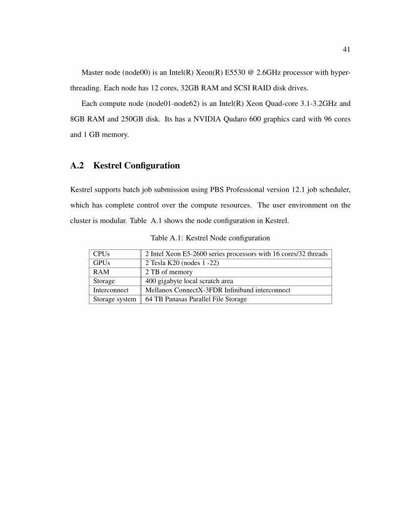
A.2 Kestrel Configuration

Kestrel supports batch job submission using PBS Professional version 12.1 job scheduler,

which has complete control over the compute resources. The user environment on the

cluster is modular. Table A.1 shows the node configuration in Kestrel.

Table A.1: Kestrel Node configuration

CPUs 2 Intel Xeon E5-2600 series processors with 16 cores/32 threadsGPUs 2 Tesla K20 (nodes 1 -22)RAM 2 TB of memoryStorage 400 gigabyte local scratch areaInterconnect Mellanox ConnectX-3FDR Infiniband interconnectStorage system 64 TB Panasas Parallel File Storage

42

Appendix B

KESTREL SCRIPTS

B.1 PBS Job Script

#!/bin/bash

### Set the job name

#PBS -N fmcwjob

### Run in the queue named "batch"

#PBS -q np_batch

### Use the bourne shell

#PBS -S /bin/sh

#PBS -V

### To send email when the job is completed:

#PBS -m ae

### Optionally set the destination for your program ’s

output

### Specify localhost and an NFS filesystem to prevent

file copy errors.

###PBS -e localhost :/home/rgeetha/hadoopjob.err

###PBS -o localhost :/home/rgeetha/hadoopjob.log

### Specify the number of cpus for your job. This

example will allocate

### 9 nodes (1 master node and 8 compute nodes)in

separate hosts with 2 cpus in each node

#PBS -l select =9: ncpus=2

#PBS -l place=vscatter:excl

### Tell PBS how much memory you expect to use. Use units

of ’b’,’kb’, ’mb’ or ’gb ’.

###PBS -l mem =20gb

#PBS -l min_walltime =00:30:00

#PBS -l max_walltime =01:00:00

43

module load java/gcc /64/1.8.0 _31

cd $PBS_O_WORKDIR

echo Working directory is $PBS_O_WORKDIR

# Calculate the number of processors allocated to this

run.

NPROCS=‘wc -l < $PBS_NODEFILE ‘

# Calculate the number of nodes allocated.

NNODES=‘uniq $PBS_NODEFILE | wc -l‘

### Display the job echo Running on host ‘hostname ‘

echo Time is ‘date ‘

echo Directory is ‘pwd ‘

echo Using ${NPROCS} processors across ${NNODES} nodes

HADOOP_HOME=$HOME/hadoop -install/hadoop

FMCWPROJECT=$HOME/MSProject/Hadoop -FMCWradar

cp ${HADOOP_HOME }/conf/masters

${HADOOP_HOME }/conf/masters.orig

cp ${HADOOP_HOME }/conf/slaves

${HADOOP_HOME }/conf/slaves.orig

rm ${HADOOP_HOME }/conf/nodes

cat $PBS_NODEFILE > ${HADOOP_HOME }/conf/nodes

sed ’s/.cm.cluster//’ ${HADOOP_HOME }/conf/nodes >

${HADOOP_HOME }/conf/pbsnodes

java -cp $HOME/hadoop -config hadoopconfig

${HADOOP_HOME }/conf/pbsnodes ${HADOOP_HOME }/conf

$HOME/hadoop -install/local -scripts/cluster -pickports.sh

55000

for line in $(cat ${HADOOP_HOME }/conf/pbsnodes) ;do

ssh -copy -id -i $HOME/.ssh/id_rsa.pub $line

ssh -x $line rm -rf /local/hadoop -‘whoami ‘*

done

pdsh -R ssh -w ^${HADOOP_HOME }/conf/slaves rm -fr

/local/hadoop -‘whoami ‘

44

pdsh -R ssh -w ^${HADOOP_HOME }/conf/slaves mkdir

/local/hadoop -‘whoami ‘

pdsh -R ssh -w ^${HADOOP_HOME }/conf/slaves chmod 700

/local/hadoop -‘whoami ‘

cd $HOME

var=‘head -1 ${HADOOP_HOME }/conf/masters ‘

echo "Creating hadoop cluster"

ssh -x $var

$HOME/hadoop -install/local -scripts/create -hadoop -cluster.sh

sleep 60

echo "Loaded data to HDFS"

ssh -x $var ${HADOOP_HOME }/bin/hadoop fs -put

$HOME/BINDATA BINDATA

ssh -x $var ${HADOOP_HOME }/bin/hadoop fs -put

${FMCWPROJECT }/ config.xml config.xml

echo "Executing fmcw hadoop job"

ssh -x $var ${FMCWPROJECT }/ FMCWradar.sh BINDATA config.xml

echo "Copying output data to local filesystem"

ssh -x $var ${HADOOP_HOME }/bin/hadoop fs -get FMCWOutput

$HOME/FMCWOutput

echo "Deleting the cluster"

ssh -x $var

$HOME/hadoop -install/local -scripts/cluster -remove.sh

pdsh -R ssh -w ^$HOME/hadoop -install/hadoop/conf/slaves

rm -fr /local/hadoop -‘whoami ‘*

B.2 Hadoop creation script#!/bin/sh

HADOOP_HOME=$HOME/hadoop -install/hadoop

if test ! -d "${HADOOP_HOME}"

then

echo

echo "Error: missing hadoop install folder:

${HADOOP_HOME}"

echo "Install hadoop in install folder before running

this script!"

45

echo

exit 1

fi

cd ${HADOOP_HOME}

rm -fr logs pids

mkdir {logs ,pids}

cd conf

for node in $(cat slaves)

do

ssh -x $node mkdir ${HADOOP_HOME }/pids/$node

ssh -x $node rm -fr /local/hadoop -‘whoami ‘

ssh -x $node mkdir /local/hadoop -‘whoami ‘

ssh -x $node chmod 700 /local/hadoop -‘whoami ‘

done

mkdir ../ pids/‘hostname ‘

B.3 Cluster removal script

#!/bin/sh

cd $HOME/hadoop -install/hadoop

echo "Warning: stopping adhoc cluster and deleting the

hadoop filesystem !!"

bin/stop -all.sh

rm -fr logs pids

echo "Removing hadoop filesystem directories"

rm -fr /local/hadoop -‘whoami ‘*