Page 1
Scholars' Mine Scholars' Mine
Masters Theses Student Theses and Dissertations
Summer 2013
3D seismic data interpretation of Boonsville Field, Texas 3D seismic data interpretation of Boonsville Field, Texas
Aamer Ali Alhakeem
Follow this and additional works at: https://scholarsmine.mst.edu/masters_theses
Part of the Geology Commons, and the Geophysics and Seismology Commons
Department: Department:
Recommended Citation Recommended Citation Alhakeem, Aamer Ali, "3D seismic data interpretation of Boonsville Field, Texas" (2013). Masters Theses. 7122. https://scholarsmine.mst.edu/masters_theses/7122
This thesis is brought to you by Scholars' Mine, a service of the Missouri S&T Library and Learning Resources. This work is protected by U. S. Copyright Law. Unauthorized use including reproduction for redistribution requires the permission of the copyright holder. For more information, please contact [email protected] .
Page 3
3D SEISMIC DATA INTERPRETATION OF BOONSVILLE FIELD, TEXAS
by
AAMER ALI ALHAKEEM
A THESIS
Presented to the Faculty of the Graduate School of the
MISSOURI UNIVERSITY OF SCIENCE AND TECHNOLOGY
In Partial Fulfillment of the Requirements for the Degree
MASTER OF SCIENCE IN GEOLOGY AND GEOPHYSICS
2013
Approved by
Dr. Kelly Liu
Dr. Stephen Gao
Dr. Yang Wan
Page 4
ii
2013
Aamer Ali Alhakeem
All Rights Reserved
Page 5
iii
ABSTRACT
The Boonsville field is one of the largest gas fields in the US located in the Fort
Worth Basin, north central Texas. The highest potential reservoirs reside in the Bend
Conglomerate deposited during the Pennsylvanian. The Boonsville data set is prepared by
the Bureau of Economic Geology at the University of Texas, Austin, as part of the
secondary gas recovery program. The Boonsville field seismic data set covers an area of
5.5 mi2. It includes 38 wells data. The Bend Conglomerate is deposited in fluvio-deltaic
transaction. It is subdivided into many genetic sequences which include depositions of
sandy conglomerate representing the potential reserves in the Boonsville field. The
geologic structure of the Boonsville field subsurface are visualized by constructing
structure maps of Caddo, Davis, Runaway, Beans Cr, Vineyard, and Wade. The mapping
includes time structure, depth structure, horizon slice, velocity maps, and isopach maps.
Many anticlines and folds are illustrated. Karst collapse features are indicated specially in
the lower Atoka. Dipping direction of the Bend Conglomerate horizons are changing
from dipping toward north at the top to dipping toward east at the bottom. Stratigraphic
interpretation of the Runaway Formation and the Vineyard Formation using well logs and
seismic data integration showed presence of fluvial dominated channels, point bars, and a
mouth bar. RMS amplitude maps are generated and used as direct hydrocarbon indicator
for the targeted formations. As a result, bright spots are indicated and used to identify
potential reservoirs. Petrophysical analysis is conducted to obtain gross, net pay, NGR,
water saturation, shale volume, porosity, and gas formation factor. Volumetric
calculations estimated 989.44 MMSCF as the recoverable original gas in-place for a
prospect in the Runaway and 3.32 BSCF for a prospect in the Vineyard Formation.
Page 6
iv
ACKNOWLEDGMENTS
First and foremost, I would like to express my sincere gratitude to my advisor Dr.
Kelly Liu for her continuous support and guidance during my research work. In addition,
I would like to spread my deep appreciation and respect to my committee members Dr.
Stephen Gao and Dr. Yang Wang; Dr. Stephen Gao for his great advices to end up with a
perfect thesis, and Dr. Yang Wang for his informative adds to my petroleum geology
understanding.
My thanks to the Saudi Ministry of Higher Education for the scholarship they
honored me with to get my master degree. Accordingly, the thanks go to my technical
advisor from Saudi Arabian Cultural Mission (SACM), Dr. Nabil Khoury. His help and
support creates the best study environment in the US.
It is a great chance to thank all my colleagues in the Department of Geological
Sciences and Engineering for motivating me. Thanks for all my officemates at McNutt
B16 who made the lab such a friendly place. Special thanks to my colleague Mr.
Abdulsaid Ibrahim for sharing helpful ideas.
I would like to thank my mother for giving me all the love that encourages me to
the success. Finally, I send tons of thanks to my lovely wife, Mrs. Hashmiah Alsaedi for
her continuous support and motivation.
Page 7
v
TABLE OF CONTENTS
Page
ABSTRACT ....................................................................................................................... iii
ACKNOWLEDGMENTS ................................................................................................. iv
LIST OF ILLUSTRATIONS ........................................................................................... viii
LIST OF TABLES ........................................................................................................... xiii
NOMENCLATURE ........................................................................................................ xiv
SECTION
1. INTRODUCTION ...................................................................................................... 1
1.1. AREA OF STUDY ............................................................................................. 1
1.2. PREVIOUS STUDIES........................................................................................ 4
1.3. OBJECTIVES ..................................................................................................... 5
2. REGIONAL GEOLOGY ........................................................................................... 6
2.1. FORT WORTH BASIN ...................................................................................... 6
2.2. GEOLOGICAL STRATIGRAPHY ................................................................. 10
2.2.1. Barnett Shale .......................................................................................... 12
2.2.2. The Bend Conglomerate. ........................................................................ 14
2.3. GEOLOGICAL STRUCTURES ...................................................................... 17
2.4. PETROLEUM SYSTEM .................................................................................. 18
2.4.1. Source Rock ........................................................................................... 18
2.4.2. Migration Pathways. ............................................................................... 18
2.4.3. Traps and Reservoirs .............................................................................. 19
3. DATA AND METHOD ........................................................................................... 22
Page 8
vi
3.1. BOONSVILLE 3D SEISMIC DATA ............................................................... 22
3.2. METHOD ......................................................................................................... 29
4. STRUCTURAL INTERPRETATION ..................................................................... 30
4.1. INTRODUCTION ............................................................................................ 30
4.2. SYNTHETIC GENERATION.......................................................................... 35
4.2.1. Time-Depth (T-D) Chart. ....................................................................... 38
4.2.2. Acoustic Impedance (AI) ....................................................................... 38
4.2.3. Wavelet. .................................................................................................. 38
4.2.4. The Reflection Coefficient (RC). ........................................................... 40
4.3. SYNTHETIC MATCHING .............................................................................. 40
4.4. HORIZON INTERPRETATION...................................................................... 43
4.4.1. Caddo and Davis .................................................................................... 43
4.4.2. Runaway and Beans Cr .......................................................................... 43
4.4.3. Vineyard and Wade ................................................................................ 44
4.4.4. Updating T-D Chart ................................................................................ 46
4.5. STRUCTURAL MAPPING ............................................................................. 47
4.5.1. Time Structure Map ................................................................................ 47
4.5.2. Average Velocity Map ........................................................................... 54
4.5.3. Depth Map. ............................................................................................. 61
4.5.4. Time to Depth Conversion. .................................................................... 71
5. STRATIGRAPHIC INTERPRETATION ............................................................... 73
5.1. HORIZON SLICE ............................................................................................ 73
5.2. ISOPACH MAP ................................................................................................ 78
Page 9
vii
5.2.1. Interval Velocity Map. ........................................................................... 78
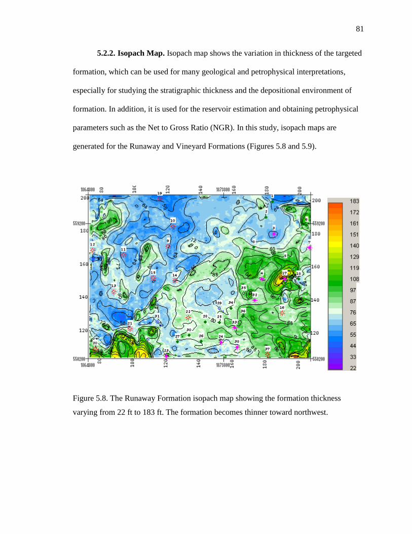
5.2.2. Isopach Map. .......................................................................................... 81
5.3. WELL LOG CORRELATION ......................................................................... 83
6. RESERVOIR ESTIMATION .................................................................................. 93
6.1. INTRODUCTION ............................................................................................ 93
6.2. ROOT-MEAN SQUARE AMPLITUDE ......................................................... 93
6.3. PETROPHYSICAL ANALYSIS ..................................................................... 96
6.3.1. Volume of Shale (Vsh) ........................................................................... 98
6.3.2. Net to Gross Ratio (NGR) .................................................................... 100
6.3.3. Porosity (Φ). ......................................................................................... 100
6.3.4. Water Saturation (Sw) .......................................................................... 102
6.3.5. Permeability (K) ................................................................................... 102
6.3.6. Gas Formation Factor (Bg) ................................................................... 103
6.4. VOLUMATRIC CALCULATION ................................................................ 106
7. CONCLUSION ...................................................................................................... 108
BIBLIOGRAPHY ........................................................................................................... 110
VITA .............................................................................................................................. 113
Page 10
viii
LIST OF ILLUSTRATIONS
Figure Page
1.1. Location of the Boonsville field and the BEG/SGR project area in the north
central of Texas (Hentz et al., 2012). ........................................................................... 2
1.2. Generalized post-Mississippian stratigraphic column for the Fort Worth Basin. ........ 3
2.1. A cross-section of a foreland basin system. ................................................................. 7
2.2. Regional paleogeography of the southern mid-continent region during the Late
Mississippian (325 Ma) showing the approximate position of the Fort Worth
Basin close to the Island Chain resulted from the convergent collision between
Laurussia and Gondwana. ............................................................................................ 7
2.3. Tectonic and structural framework of the Fort Worth Foreland Basin. ....................... 8
2.4. Paleogeology and structural elements of the Fort Worth Basin showing the
depositional environment formed the Bend Conglomerate (Thomas et al., 2003). ..... 9
2.5. North-south and west-east cross sections through the Fort Worth Basin
illustrating the structural position of the Barnett Shale between the Muenster
Arch, Bend Arch, and Llano Uplift (Burner et al., 2011). ......................................... 10
2.6. Generalized subsurface stratigraphic section of the Bend Arch–Fort Worth Basin
province showing the distribution of source rocks, reservoir rocks, and seal
rocks of the Barnett-Paleozoic petroleum system (Pollastro et al., 2003). ................ 11
2.7. Structure contour map on top of the Barnett Shale, Bend arch–Fort Worth Basin. .. 13
2.8. Stratigraphic nomenclature used to define the Bend Conglomerate genetic
sequences in the Boonsville field. .............................................................................. 15
2.9. Composite genetic sequence illustrating the key chronostratigraphic surfaces and
typical facies successions. .......................................................................................... 16
2.10. The major geological features bounding the Fort Worth Basin. .............................. 20
2.11. Petroleum system event chart for Barnett-Paleozoic total petroleum system of
the Fort Worth Basin, Texas. ..................................................................................... 21
Page 11
ix
3.1. Basemap of the 3D seismic data set of the Boonsville field, north central Texas. .... 23
3.2. Chart showing the logs provided with each well. ...................................................... 26
4.1. Vertical seismic section of Crossline 147 showing a general view of the seismic
data. ............................................................................................................................ 31
4.2. Time slice at 1.062 s showing a general view of the seismic data. ............................ 32
4.3. General view of the structural geology using the formation tops. ............................. 33
4.4. The interpretation work flow. .................................................................................... 34
4.5. Synthetic seismogram generation for Well BY18D, illustrating all the
components used and the synthetic seismogram generated. ...................................... 36
4.6. Synthetic seismogram generation for Well 14 (BY15), illustrating all the
components used and the synthetic seismogram generated. ...................................... 37
4.7. Extracted wavelets and their amplitude spectra for Wells 15 and 14. ....................... 39
4.8. Seismic section of Crossline 151 with the generated synthetic seismograms from
Well 15 (BY18D). ...................................................................................................... 41
4.9. Seismic section of Crossline 152 with the generated synthetic seismograms from
Well 15 (BY18D) (green), and Well 14 (BY15) (blue). ............................................ 42
4.10. Seismic section of Inline112 showing the horizon picking for: Caddo (MFS90)
in blue, Davis (MFS70) in pink, Runaway (MFS53) in yellow, Beans Creek
(MFS40) in light brown, Vineyard (MFS20) in green, and Wade (MFS10) in
dark green. .................................................................................................................. 45
4.11. Time structure map of the Caddo top (MFS90) showing a dipping toward
north. .......................................................................................................................... 48
4.12. Time structure map of the Davis top (MFS70) showing a dipping toward north. ... 49
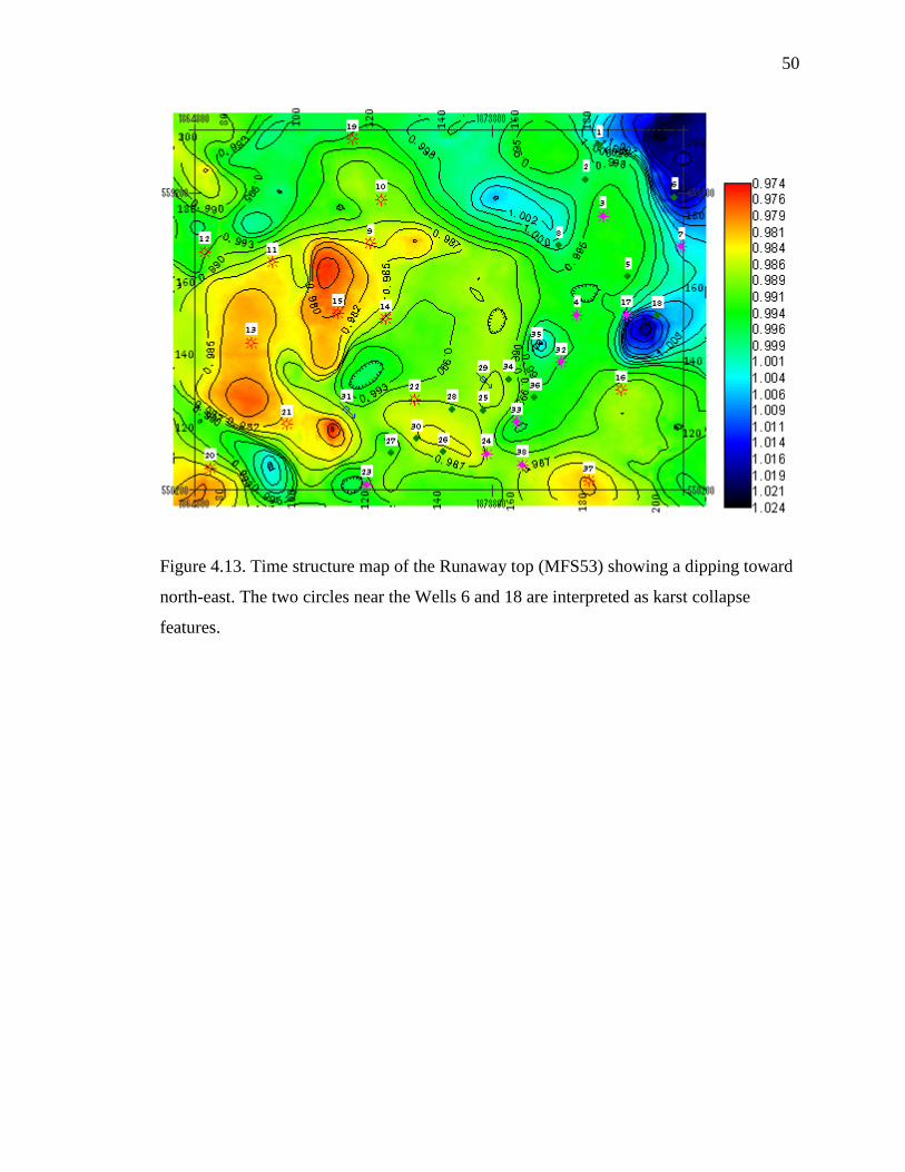
4.13. Time structure map of the Runaway top (MFS53) showing a dipping toward
north-east. ................................................................................................................... 50
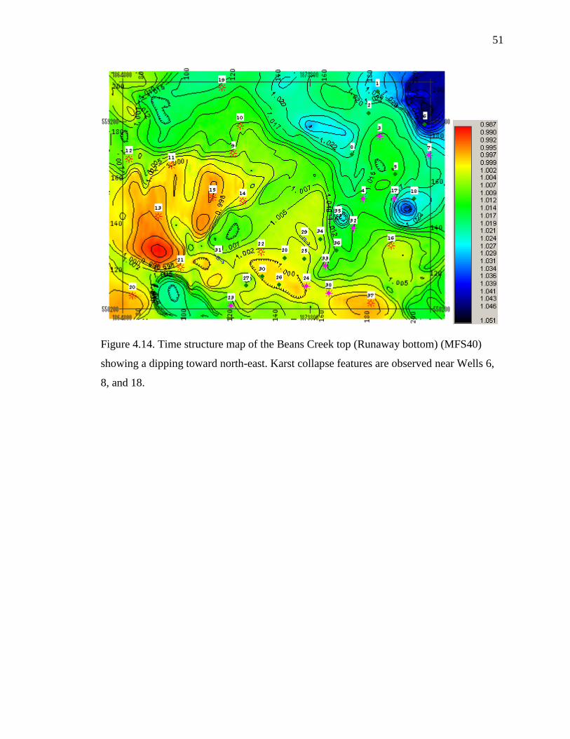
4.14. Time structure map of the Beans Creek top (Runaway bottom) (MFS40)
showing a dipping toward north-east. ........................................................................ 51
Page 12
x
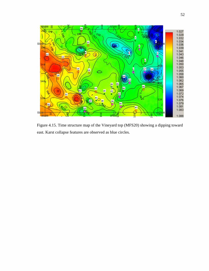
4.15. Time structure map of the Vineyard top (MFS20) showing a dipping toward
east. ............................................................................................................................ 52
4.16. Time structure map of the Wade top (Vineyard bottom) (MFS10) showing a
dipping toward east. ................................................................................................... 53
4.17. Illustration showing the method to compute the parameters from the well
formation top and the seismic time structure in order to calculate the average
velocity. ...................................................................................................................... 54
4.18. Average velocity map of the Caddo (MFS90). ........................................................ 55
4.19. Average velocity map of the Davis (MFS70). ......................................................... 56
4.20. Average velocity map of the Runaway (MFS53). ................................................... 57
4.21. Average velocity map of the Beans Cr top (Runaway base) (MFS40).................... 58
4.22. Average velocity map of the Vineyard (MFS20). ................................................... 59
4.23. Average velocity map of the Wade top (Vineyard base) (MFS10). ........................ 60
4.24. The Caddo (MFS90) depth map in TVD from the seismic datum (ft) showing
that the layer is dipping toward north. ....................................................................... 62
4.25. The Davis (MFS70) depth map in TVD from the seismic datum (ft) showing
that the layer is dipping toward north. ....................................................................... 63
4.26. The Runaway (MFS53) depth map in TVD from the seismic datum (ft)
showing that the layer is dipping toward north-east. ................................................. 64
4.27. The Bean Cr (MFS40) depth map in TVD from the seismic datum (ft) showing
that the layer is dipping toward north-east. ................................................................ 65
4.28. The Vineyard (MFS20) depth map in TVD from the seismic datum (ft)
showing that the layer is dipping toward north-east. ................................................. 66
4.29. The Wade (MFS10) depth map in TVD from the seismic datum (ft) showing
that the layer is dipping toward east. ......................................................................... 67
4.30. 3D structure depth view for all the targeted formations. ......................................... 68
Page 13
xi
4.31. 3D depth structure view of the Runaway Formation top (MFS53) and base
(MFS40). .................................................................................................................... 69
4.32. 3D depth structure view of the Vineyard Formation top (MFS20) and base
(MFS10). .................................................................................................................... 70
4.33. Vertical seismic section in depth. ............................................................................ 72
5.1. The Runaway top (MFS53) horizon slice indicating a channel by the high
amplitudes. ................................................................................................................. 74
5.2. Horizon slice for the Beans Cr (MFS40), base of Vineyard, indicating a channel
flowing toward southwest. ......................................................................................... 75
5.3. Top Vineyard (MFS20) horizon slice showing a channel indicated by the high
amplitudes from the south to north. ........................................................................... 76
5.4. Horizon slice of the Wade (MFS10), the Vineyard Base showing the effect of
karst collapse features at the base of the Bend Conglomerate near the Wells 6, 8,
18, 27, 33, and 35. ...................................................................................................... 77
5.5. Illustration showing the method to compute the parameters from the well
formation tops and the seismic time structure in order to calculate the interval
velocity. ...................................................................................................................... 78
5.6. The Runaway Formation interval velocity map. ........................................................ 79
5.7. The Vineyard Formation interval velocity map. ........................................................ 80
5.8. The Runaway Formation isopach map showing the formation thickness varying
from 22 ft to 183 ft. .................................................................................................... 81
5.9. The Vineyard Formation isopach map showing the formation thickness varying
from 34 ft to 230 ft. .................................................................................................... 82
5.10. GR and Rt logs showing in the basemap for the Runaway Formation. ................... 84
5.11. GR and Rt logs showing in the basemap for the Vineyard Formation. ................... 85
5.12.Well log correlation for the Runaway Formation. .................................................... 86
5.13. Well log correlation for the Runaway Formation .................................................... 87
Page 14
xii
5.14. SP-Rt log from the Well 2 showing in the seismic section for the Runaway
Formation. .................................................................................................................. 88
5.15. GR (green) and Rt (blue) logs from the Well 19 showing in the seismic section
of crossline 199. ......................................................................................................... 89
5.16. Rt logs for the Wells 2, 4 and 37 plotted in the seismic section. ............................. 90
5.17. Well log correlation for the Vineyard Formation. ................................................... 91
5.18. Well logs placed in the vertical seismic section for the Vineyard Formation. ........ 92
6.1. RMS amplitude map of the Runaway Formation with the depth structural
contour of the Runaway top. ...................................................................................... 94
6.2. RMS amplitude map of the Vineyard Formation with the depth structural
contour of the Vineyard top. ...................................................................................... 95
6.3. Logs generated from the Rt (RILD) log of the Well 2. ............................................. 97
6.4. SP logs for the Wells 2 and 16 showing examples for calculating the SPcln by
7% cut off and calculating SPsh by 10% cut off. ...................................................... 99
6.5. Well 2 logs generated from the petrophysical analysis showing the shale volume
(Vsh) and effective porosity (PHIE). ....................................................................... 104
6.6. Well 16 logs generated from the petrophysical analysis showing the shale
volume (Vsh) and effective porosity (PHIE). .......................................................... 105
Page 15
xiii
LIST OF TABLES
Table Page
2.1. The Bend Conglomerate reservoir properties (Hardage et al., 1996) ........................ 17
3.1. Coordinators defining the study area in the Boonsville field (Hardage et al.,
1996) .......................................................................................................................... 24
3.2. Vibroseis velocity survey in the Billie Yates 18D well (Hardage et al., 1996) ......... 25
3.3. Dynamite velocity survey in the Billie Yates 18D well (Hardage et al., 1996) ........ 25
3.4. Well data and formation tops of MFS depths (ft) measured relative to KB
(Hardage et al., 1996) ................................................................................................. 28
3.5. The SMT Kingdom Suite 8.6 modules used in the study .......................................... 29
4.1. Updated T-D charts generated from the horizon picks and the formation tops. ........ 46
6.1. Calculated reservoir properties from the Runaway Formation .................................. 96
6.2. Calculated reservoir properties from the Vineyard Formation .................................. 96
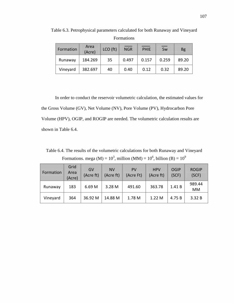
6.3. Petrophysical parameters calculated for both Runaway and Vineyard Formations 107
6.4. The results of the volumetric calculations for both Runaway and Vineyard
Formations. .............................................................................................................. 107
Page 16
xiv
NOMENCLATURE
Symbol Description
3D Three Dimensional
AI
bbl
Acoustic Impedance
Barrel
BEG Bureau of Economic Geology
CALI Caliper
CC Correlation Coefficient
CS Check Shot
DT Delta-t Sonic
GR Gamma Ray
GRI Gas Research Institute
KB
LL3
Kelly Bushing
Laterolog 3 Resistivity
LL8 Laterolog 8 Resistivity
LAT Laterolog Resistivity
LN Long Normal Resistivity
LVM Local Varying Mean
mi2
MICRO
Mile Square
Micro Log
MLP Multi-Layer Perception
MSFL Micro Spherically Focused Log
NPHI Compensated Neutron
TWT Two Way Time
PEF Photo Electric Effect
RILD Deep Induction Resistivity
RILM Medium Induction Resistivity
RC Reflection Coefficient
RHOB Bulk Density
SFL Spherically Focused Resistivity
SGR Secondary Gas Recovery
SN Short Normal (16”) Resistivity
Page 17
xv
SRD
Tcf
HST
LST
TST
Seismic Reference Datum
Trillion Cubic Feet
Highstand
Lowstand
Transgressive
Page 18
1. INTRODUCTION
1.1. AREA OF STUDY
The Boonsville field is located, primarily, within both Wise County and Jack
County in Texas (Figure 1.1). It encompasses approximately 2300 mi2 in the Fort Worth
Basin, North central Texas (Hardage et al., 1996). This field is considered as one of the
largest gas fields in the United States, especially, from the Bend Conglomerate group,
which was deposited during the Atoka Stage of the Middle Pennsylvanian period
(Hardage et al., 1996) (Figure 1.2). As of January 2011, the lower Atoka reservoirs,
collectively, produced more than 3.2 tcf (trillion cubic feet) of natural gas and more than
36.3 million bbl (barrel) of oil from more than 5700 wells (IHS Energy, Inc., 2011).
A 3D seismic exploration acquisition was conducted in the Boonsville field for a
Secondary Gas Recovery (SGR) program which was funded by the U.S. Department of
Energy and the Gas Research Institute (GRI) from 1993 to 1996. The exploration
covered a total area of 26 mi2 (Hardage et al., 1996).
The Bureau of Economic Geology (BEG) at the University of Texas, Austin
prepared a Boonsville 3D seismic data set as part of the SGR, supported by the GRI. This
data is a result of three companies who operated the area of SGR and worked side by side
with BEG. The companies are Arch Petroleum, Enserch, and OXY, those who paid 90%
of the 3D seismic Data acquisition and processing cost (Hardage et al., 1996).
The primary targeted reservoirs in the Boonsville field are in the Bend
Conglomerate Formation (Hardage et al., 1996). These reservoirs hold high content of
gas and some oil. During the Atoka stage, the Bend Conglomerate was deposited in a
fluvio-deltaic transition environment (Hardage et al., 1996). An important feature in this
Page 19
2
field is karst collapse zones, which occurred as a result of collapsing of the deep
Ellenburger carbonate formation (Hardage et al., 1996).
Figure 1.1. Location of the Boonsville field and the BEG/SGR project area in the north
central of Texas (Hentz et al., 2012).
Page 20
3
Figure 1.2. Generalized post-Mississippian stratigraphic column for the Fort Worth
Basin. In the Boonsville field, the Bend Conglomerate which is shown during Atokan
series, is equivalent to the Atoka Group (Hardage et al., 1996).
Page 21
4
1.2. PREVIOUS STUDIES
Boonsville field, which lies in the Fort Worth Basin in the north-central of Texas,
is one of the largest gas reserves in US. It contains many potential formations within a
complete petroleum system. As a result, many studies were conducted using the
Boonsville 3D seismic data set.
Since 1985, Hardage and colleagues (Hardage et al., 1996) have conducted
extensive studies for the Boonsville field. These studies include the seismic
interpretations and reservoir characterization in the Bend Conglomerate. The studies
resulted both geologic understanding and petrophysical analysis to the Boonsville field.
Discontinuous and thin reservoirs were identified. In addition, some approaches were
developed to characterize the reservoir geometries for the gas reserves. The effects of the
carbonate karst collapse were also recognized.
Using core data, seismic data, and well logs, Maharaj et al. (2009) identified the
facies in Atoka based on lithological relationships. The study divided Atoka into twelve
parasequences and identified point bars and channels.
Hentz et al. (2012) mapped sandstone distribution of the depositional facies using
the well log chronostatigrapic framework. This study provided depositional geometries of
Atoka. It suggested that the Bend includes braided fluvial deposits, braid-plain deposits,
and river-dominated deltas.
Page 22
5
1.3. OBJECTIVES
The objective of this study is to provide a geological visualization of the
Boonsville field subsurface by correlating the regional geological data, geophysical
seismic data, well logs, well test data, and well production history. Geologic subsurface
structures were visualized for six horizons within the Bend Conglomerate. The horizons
are Caddo, Davis, Runaway, Beans Creek, Vineyard, and Wade. Various maps such as
time structure, horizon slice, velocity, depth structure, and isopach were constructed.
Moreover, the seismic data volume was converted from time to depth domain for better
correlation with well logs.
Another objective includes stratigraphic interpretation to identify different
geological features for both the Runaway and Vineyard Formations. Studying the horizon
slices, isopach maps, and well logs were useful to interpret the stratigraphic features such
as fluvial dominated channels, point bars, and mouth bar sandstone deposits.
Reservoirs estimation is conducted for the Runaway and the Vineyard
Formations. First, RMS amplitude maps were generated as a direct hydrocarbon indicator
to show bright spots. Then, petrophysical analyses were implemented for both formations
to conduct the reservoir properties and to calculate petrophysical parameters including
the gross, net pay, NGR, water saturation, shale volume, porosity, and gas formation
factor. Two prospects are identified for both formations. Finally, volumetric prospect
calculations were performed to estimate the amount of the recoverable original gas in-
place (ROGIP) for the Runaway Formation and the Vineyard Formation.
Page 23
6
2. REGIONAL GEOLOGY
2.1. FORT WORTH BASIN
Fort Worth Basin is a part of the foreland basin system (Figure 2.1). This basin
was formed during Late Paleozoic episode deformed along the Ouachita Fold-Thrust belt
(Figure 2.2). It has an area of approximately 15000 mi2 (Walper, 1982; Thompson, 1988)
and elongates north-south parallel to the Ouachita Thrust fault located in the south-east of
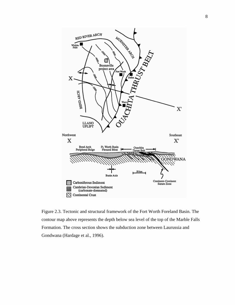
the basin. The Fort Worth Basin is bounded by the Muenster Arch to the east-north, the
Red River Arch to the north-west, the structural Bend Arch to the west, and the
Precambrian Llano uplift to the south (Figure 2.3).
The Fort Worth Basin deposited during the formation of Pangea as a foredeep
basin within the foreland basin system (Walper, 1982) (Figure 2.1). In Early Paleozoic,
carbonate deposition from Cambro-Ordivician followed by erosion during the Middle
Paleozoic. The basin is developed between the Ouachita Thrust Belt and the Bend Arch
during the tectonic plate convergence between Laurussia plate and Gondwana plate
(Figures 2.2 and 2.3). During Mississippian-Pennsylvanian, the Ouachita Thrust Belt
developed as a result of plate convergence when the continental margin was approaching
the subduction zone (Figure 2.3). Subsequently during Pennsylvanian, the Fort Worth
Basin formed when layering sequence deposited on the continental margin (Walper,
1982) (Figure 2.4).
Page 24
7
Figure 2.1. A cross-section of a foreland basin system. The Fort Worth Basin is
considered as a foredeep basin within a foreland basin system (Modified from DeCelles
and Giles, 1996).
Figure 2.2. Regional paleogeography of the southern mid-continent region during the
Late Mississippian (325 Ma) showing the approximate position of the Fort Worth Basin
close to the Island Chain resulted from the convergent collision between Laurussia and
Gondwana. Llano Uplift and the Arch equator are shown. They played important rule in
the evaluation of the Fort Worth Basin (Burner et al., 2011).
Page 25
8
Figure 2.3. Tectonic and structural framework of the Fort Worth Foreland Basin. The
contour map above represents the depth below sea level of the top of the Marble Falls
Formation. The cross section shows the subduction zone between Laurussia and
Gondwana (Hardage et al., 1996).
Page 26
9
During Early Atoka, the Muenster Arch was the primary sediment source that
formed and served the Fort Worth Basin. In addition, the Ouachita Fold Belt and the
Bend Arch also fed the Fort Worth Basin as sediment sources (Figure 2.4). They
deformed the Fort Worth Basin into the warped shape (Thomas, 2003). The Llano Uplift,
worked as the main structure that twisted the formations of the Fort Worth Basin to its
present structure and dip (Figure 2.5). The Fort Worth Basin is shallow, and dipping
toward the north, with a maximum depth of 12000 ft along the Ouachita (Burner et al.,
2011) (Figure 2.5).
Figure 2.4. Paleogeology and structural elements of the Fort Worth Basin showing the
depositional environment formed the Bend Conglomerate (Thomas et al., 2003).
Page 27
10
Figure 2.5. North-south and west-east cross sections through the Fort Worth Basin
illustrating the structural position of the Barnett Shale between the Muenster Arch, Bend
Arch, and Llano Uplift (Burner et al., 2011).
2.2. GEOLOGICAL STRATIGRAPHY
During the Pennsylvanian Period, different sequences of sedimentary deposition
were accumulated in the Fort Worth Basin. Depositions of 6000 – 7000 ft consist mainly
of clastics and carbonates. However, accumulations from Ordovician – Mississippian
comprise about 4000 – 5000 ft of carbonates and shales (Burner et al., 2011; Thompson,
1988) (Figure 2.6).
Page 28
11
Figure 2.6. Generalized subsurface stratigraphic section of the Bend Arch–Fort Worth
Basin province showing the distribution of source rocks, reservoir rocks, and seal rocks
of the Barnett-Paleozoic petroleum system (Pollastro et al., 2003).
Page 29
12
2.2.1. Barnett Shale Barnett Shale is an important Formation in the Fort Worth
Basin. It plays a critical role in forming different gas fields in the northern part of Texas
(Pollastro et al., 2007). Barnett shale consists of the Mississippian petroliferous black
shale (Burner et al., 2011). It is considered to be a primary Kerogen kitchen in the Fort
Worth Basin (Pollastro et al., 2007). It feeds the Pennsylvanian clastic reservoirs in the
Boonsville field. Moreover, Barnett Shale represents an unconventional hydrocarbon play
where the main elements of a petroleum system are found. Kerogen source, reservoir, and
seal coincide in the same Formation. As a result, Barnett Shale is targeted itself (e.g., the
Newark East field, where the Formation is 300-500 ft thick and 6500-8500 ft deep
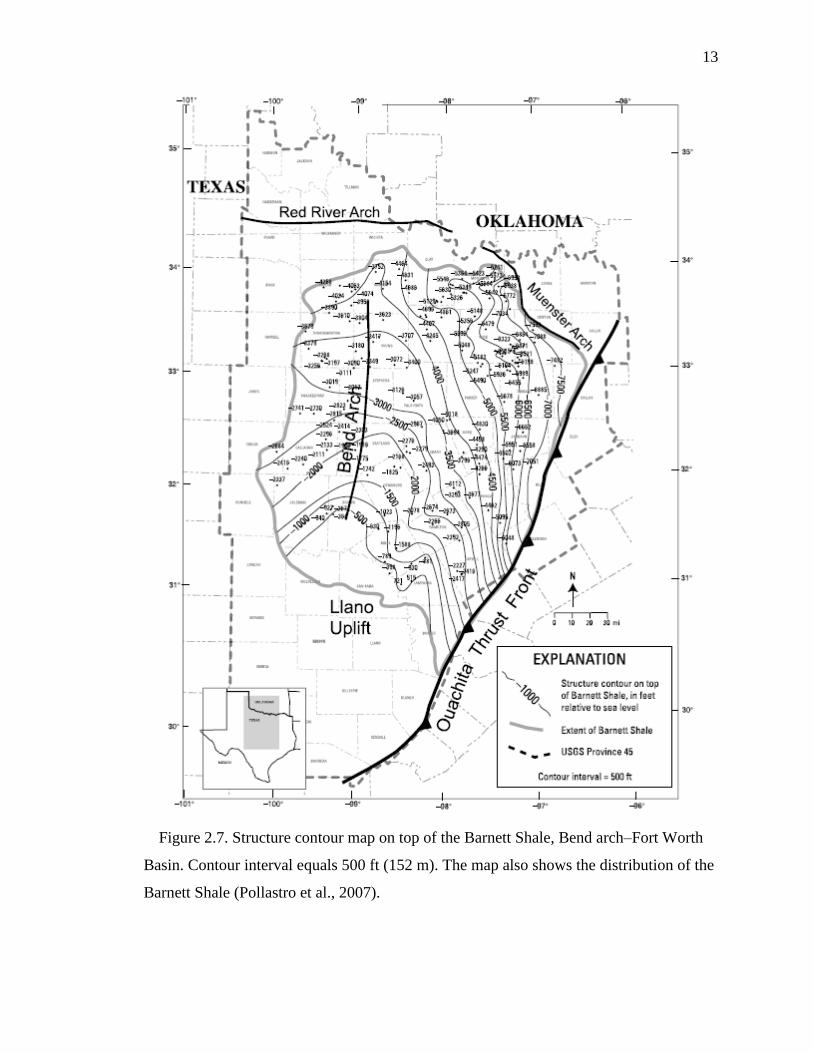
(Burner et al., 2011) (Figure 2.7).
Page 30
13
Figure 2.7. Structure contour map on top of the Barnett Shale, Bend arch–Fort Worth
Basin. Contour interval equals 500 ft (152 m). The map also shows the distribution of the
Barnett Shale (Pollastro et al., 2007).
Page 31
14
2.2.2. The Bend Conglomerate. The Bend Conglomerate is an interval of the
Atoka group deposited in the Fort Worth Basin during the Middle Pennsylvanian. It
consists of many genetic sequences characterized by Conglomerate depositions (Figure
2.8). It is deposited in fluvial – deltaic transition environment (Hardage et al., 1996).
Each genetic sequence represents one relative base level cycle. Each cycle is
characterized by highstand (HST), lowstand (LST), and transgressive (TST) system
tracts. Reservoir sandstone facies, regularly, arise in the LST. The Bend includes braided
fluvial deposits, braid-plain deposits, and river-dominated deltas (Hentz et al., 2012).
These environments resulted high porous, thin, and discontinuous formations of
Conglomerate sandstone formed within a genetic sequences shown by a stratigraphic
nomenclature in Figure 2.8. The Bend Conglomerate genetic sequence of depositional
environment is identified by Galloway (1989) termed as following: the Maximum
Flooding Surface (MFS), the Flooding Surface (FS), and the Erosional Surface (ES)
(Figure 2.9). The Bend begins at the Caddo Formation and ends at the Vineyard
Formation. There are erosional surfaces between the formations giving a precise
definition of the clastic reservoirs. Because of their high productivity, both the Caddo and
Vineyard Formations are the main target zones in the Boonsville field (Hardage et al.,
1996). Table 2.1 lists the Bend Conglomerate reservoir properties.
Page 32
15
Figure 2.8. Stratigraphic nomenclature used to define the Bend Conglomerate genetic
sequences in the Boonsville field. As defined by the Railroad Commission of Texas, the
Bend Conglomerate is the interval from the base of the Caddo Limestone to the top of the
Marble Falls Limestone (Hardage et al., 1996).
Page 33
16
Figure 2.9. Composite genetic sequence illustrating the key chronostratigraphic surfaces
and typical facies successions. It is constructed from the actual core data spanning four
Bend Conglomerate sequences. One relative base level cycle is commonly represented by
HST, LST, and TST systems tracts. Cycles begin and end with MFS and typically
contains one or more ES and FS, which are commonly ravinement surfaces (Hardage et
al., 1996).
Page 34
17
Table 2.1. The Bend Conglomerate reservoir properties (Hardage et al., 1996)
2.3. GEOLOGICAL STRUCTURES
The Boonsville field was developed with different types of structural features,
which are the result of either tectonic activity or solution weathering. An important
structural feature in this area is the Mineral Wells Fault. It runs northeast-southwest with
a length of more than 65 mi. In addition, there are many high-angle normal faults, karst
fault chimneys, and local subsidence in the Boonsville field (Hardage et al., 1996). This
is related to the karst development and solution collapse in the underlying Ordovician
Ellenburger Group (Hardage et al., 1996). The karst collapse features extend vertically
upward 2500 - 3500 ft through the strata of Barnet, Marble falls, and the Atoka group
with diameters ranging from 1640 to 3940 ft (McDonnell et al., 2007).
Property/item Typical values
Depth 4500 to 6000 ft
Initial pressures 1400 to 2200 psi – somewhat underpressured
Temperature 150ºF
Gas gravity 0.65 to 0.75
Gross thickness 900 to 1300 ft
Net thickness Multiple pays from a few ft to 20–30 ft each
Permeability Varies from <0.1 md to >10 md; 0.1 to 5 md typical
Porosity 5 to 20 %
Production From 10 Mmscf to 8 Bscf; 1.5 Bscf Median
Page 35
18
2.4. PETROLEUM SYSTEM
The Boonsville field is a result of a complete petroleum system occurring north of
the Fort Worth Basin. It consists of mature source rocks, migration pathways, reservoir
rocks, and seals. The petroleum system elements in the Boonsville field are described as
following:
2.4.1. Source Rock. The Barnett Shale is proved to be the primarily source rock
for the hydrocarbon accumulation in the Bend Conglomerate (Hardage et al., 1996;
Pollastro et al., 2003) (Figure 2.6). Figure 2.10 illustrates the distribution of the Barnett
Shale in the Fort Worth Basin and the location of the Boonsville field. The Barnett Shale
consists of shale and limestone. The shale properties are dense, organic-rich, soft, thin-
bedded, petroliferous, and fossiliferous. The limestone properties are hard, black, finely
crystalline, petroliferous, and fossiliferous. The Barnett kerogen is type II, with a minor
admixture of type III (Burner et al., 2011) (Figure 2.11).
2.4.2. Migration Pathways. There are some major faults proven to be the
hydrocarbon migration pathways in the Boonsville field. The Mineral Wells Fault system
is a suggested pathway to migrate the hydrocarbon from the Barnett Shale up to Atoka. In
addition, karst features are approved as high efficient pathways (Hardage et al., 1996;
Pollastro et al., 2007). These features extend in the Fort Worth Basin through the
Mississippian to the Pennsylvanian strata. Accordingly, the karst collapses connect the
Barnett Shale and other thin shale beds in the Atoka to the Bend Conglomerate
reservoirs. These karst collapses work as high efficient migration pathways for the
hydrocarbon.
Page 36
19
2.4.3. Traps and Reservoirs. The Bend Conglomerate consists of porous and
permeable conglomerate sandstone formations. Point bars and channel depositions are
part of the genetic sequences of the Bend. These depositions are bounded by erosional
sequences. High potential reservoirs are founded in the following main zones of the
Bend: Caddo, Davis, Runaway, and Vineyard (Hardage et al., 1996) (Figure 2.8). Shale
and mudstone layers are deposited at the end of LST. These layers bound different
sandstone formations of the Bend Conglomerate (Figure 2.9).
Page 37
20
Figure 2.10. The major geological features bounding the Fort Worth Basin. The blue
color outlines the extent of the Barnett Shale. The gas reserve north of the Fort Worth
Basin (green) represents the Boonsville field (Burner et al., 2011).
Page 38
21
2.1
1. P
etro
leum
syst
em e
ven
t ch
art
for
Bar
net
t-P
aleo
zoic
tota
l p
etro
leum
syst
em o
f th
e F
ort
Wort
h B
asin
, T
exas
.
Abb
revia
tions:
E =
Ear
ly;
M =
Mid
dle
; L
= L
ate;
Cam
= C
ambri
an;
Ord
= O
rdovic
ian;
Sil
= S
iluri
an;
Dev
= D
evonia
n;
Mis
= M
issi
ssip
pia
n;
Pen
= P
ennsy
lvan
ian;
Per
= P
erm
ian;
Tr
= T
rias
sic;
Jur
= J
ura
ssic
; C
ret
= C
reta
ceous;
Ter
= T
erti
ary;
Cen
= C
enozo
ic;
O =
Oli
goce
ne;
Mi
= M
ioce
ne
(Poll
astr
o e
t al
., 2
007).
Fig
ure
Page 39
22
3. DATA AND METHOD
3.1. BOONSVILLE 3D SEISMIC DATA
The data used in this project is the BEG/SGR 3D seismic data set of the
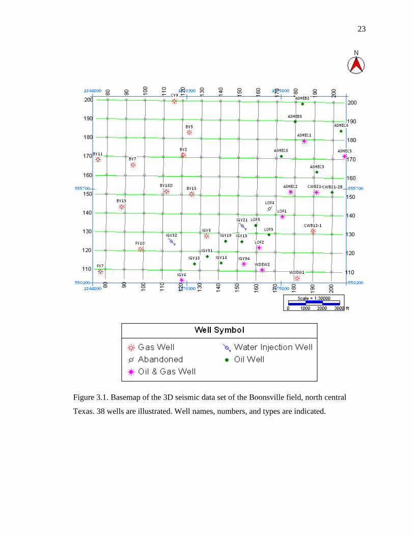
Boonsville field, north central Texas. This data includes a 3D seismic survey, 38 wells,
well logs, formation tops, production test data, checkshots, and a Vertical Seismic Profile
(VSP). The 3D seismic data covers an area of 5.5 mi2 out of 26 mi
2, the total SRG
Boonsville study area (Figure 3.1). The source for the seismic survey was 10 oz
directional explosives and the sampling rate was 1 ms. The survey source and receiver
lines were staggered, allowing for a high-fold number, with 110 X 110-ft bins (Hardage
et al., 1996). The 3D seismic volume was processed by Trend Technology of Midland,
Texas. Hardage (1996) summarized the seismic processing sequence as following:
1. Surface and subsurface maps
2. Geometry definition and application
3. Prefilter 17-250 Hz
4. Surface-consistent deconvolution
5. Refraction statics: Seismic datum = 900 ft, velocity = 8000 ft/s
6. Velocity analysis
7. Refraction statics: Seismic datum = 900 ft, velocity = 8000 ft/s
8. CDP stack
9. Automatic residual statics: Iterate 6 times
10. Velocity analysis
11. Normal moveout
12. Spectral balance
13. CDP residual statics
14. CDP stack (55- and 110-ft bins)
15. Interpolate missing CDPs at edges of data volume (55-ft bins only)
16. 3-D migration
Page 40
23
Figure 3.1. Basemap of the 3D seismic data set of the Boonsville field, north central
Texas. 38 wells are illustrated. Well names, numbers, and types are indicated.
Page 41
24
This 3D seismic volume consists of 110 ft stacking bins. Trace (Inline,X) values
increase from west to east and line (Crossline,Y) values increase from south to north. The
northeast corner is located at Trace 206, Line 201. The southwest corner of the survey is
located at Trace 74, Line 105. The longitude and latitude values for the four corners of
the survey were translated to X and Y values for the North Central Texas Zone (4202) of
the U. S. State Plane Coordinate System and the 1927 North American Datum. Table 3.1
lists the corners, starting in the southwest corner and moving clockwise. The Boonsville
3D seismic SEGY file text header is listed as following:
Line number in bytes 9 – 12 105 – 201
Trace number in bytes 21 – 24 74 – 206
97 lines with 133 traces each
32 bit IBM Floating point data
Samples at 1 millisecond sampling rate
The maximum amplitude value is 149035.5.
The minimum amplitude value is 32029.25.
The average amplitude value is 63670.67.
Table 3.1. Coordinators defining the study area in the Boonsville field (Hardage et al.,
1996)
Trace Line Longitude Latitude X Location Y Location
74
74
206
206
105
201
201
105
-97.94162
-97.94132
-97.89384
-97.89416
33.17897
33.20800
33.20766
33.17863
1864886
1865021
1879540
1879406
550461
561020
560838
550279
Page 42
25
The 38 well data includes various logs such as resistivity, gamma ray, SP, sonic,
neutron, and density logs. Billie Yates 18D well is provided with the vibroseis-source
VSP data and explosive (dynamite) checkshots as seen in Tables 3.2 and 3.3. Figure 3.2
shows types of logs included in each well. The resistivity and SP are the most log type
available.
Table 3.2. Vibroseis velocity survey in the Billie Yates 18D well (Hardage et al., 1996)
Level Depth KB (ft)
Vertical Depth from
SRD (ft)
Measured one-way time
(ms)
Vertical one-way time from source
(ms)
Vertical one-way time from SRD
(ms)
1 1000 8850 123 115.9 97
2 2000 1850 212.8 209.5 190.6
3 2500 2350 258.2 255.6 236.7
4 3000 2850 300.9 298.8 279.9
5 3500 3350 342.5 340.7 321.9
6 4000 3850 385.3 383.8 364.9
7 4500 4350 426.2 424.9 406
8 5000 4850 467.9 466.7 447.8
9 5500 5350 508.3 508.2 489.2
10 5700 5550 524.7 523.7 504.8
Table 3.3. Dynamite velocity survey in the Billie Yates 18D well (Hardage et al., 1996)
Level Depth KB (ft)
Vertical Depth from
SRD (ft)
Measured one-way time
(ms)
Vertical one-way time from source
(ms)
Vertical one-way time from SRD
(ms)
1 1000 850 117.4 107.3 91.1
2 2000 1850 205.2 200.4 184.2
3 2500 2350 250.3 246.6 230.3
4 3000 2850 291.5 288.5 272.2
5 3500 3350 332.7 330.1 313.8
6 4000 3850 374.4 372.2 356
7 4500 4350 414.8 412.9 396.7
8 5000 4850 456.2 454.5 438.2
9 5500 5350 485.4 493.8 477.6
10 5723 5573 514.3 512.8 496.5
Page 43
26
Figure 3.2. Chart showing the logs provided with each well. Red color indicates
resistivity logs. All wells have resistivity log and SP log. Log abbreviations can be found
in the nomenclature page.
0 1 2 3 4 5 6 7 8 9 10 11 12
ASHEB2ASHEB3ASHEC1ASHEC2ASHEC3ASHEC4ASHEC5ASHEC6
BY2BY3BY7
BY11BY13BY15
BY18DCWB12-1CWB21-1
CWB21-2BCY9FY7
FY10IGY3IGY4
IGY9AIGY13IGY14IGY18IGY19IGY21IGY31IGY32LOF1LOF2LOF3LOF4LOF5
WDEW1WDEW2
RILD
RILM
SFL
LL3
LL 8
S GRD
SN
LN
LAT
SP
GR
NPHI
RHOB
PEF
DELT
MICRO
CALI
MSFL
Page 44
27
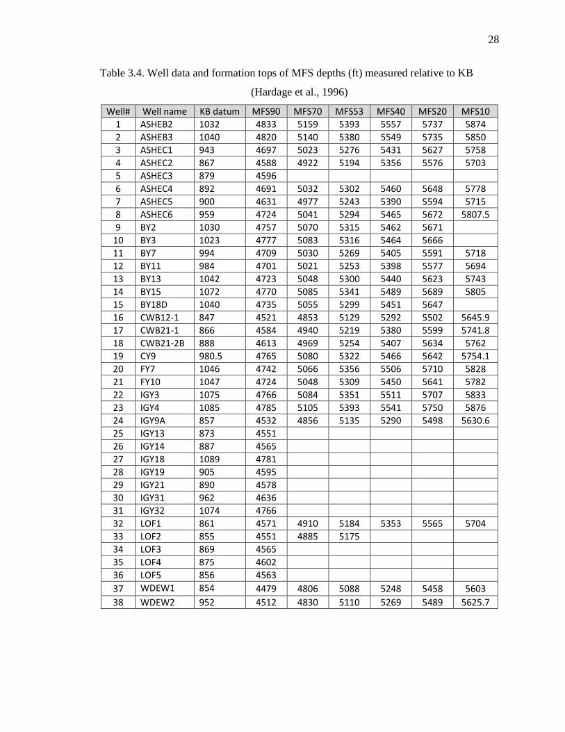
Formation tops are provided for the wells. All the MFS, FS, and ES top depths are
provided for all formations in the Bend Conglomerate. Table 3.4 lists the genetic
sequence boundaries of MFS depths in each well for the formations that are interpreted in
this study, depths from Kelly Bushing (KB).
Page 45
28
Table 3.4. Well data and formation tops of MFS depths (ft) measured relative to KB
(Hardage et al., 1996)
Well# Well name KB datum MFS90 MFS70 MFS53 MFS40 MFS20 MFS10
1 ASHEB2 1032 4833 5159 5393 5557 5737 5874
2 ASHEB3 1040 4820 5140 5380 5549 5735 5850
3 ASHEC1 943 4697 5023 5276 5431 5627 5758
4 ASHEC2 867 4588 4922 5194 5356 5576 5703
5 ASHEC3 879 4596
6 ASHEC4 892 4691 5032 5302 5460 5648 5778
7 ASHEC5 900 4631 4977 5243 5390 5594 5715
8 ASHEC6 959 4724 5041 5294 5465 5672 5807.5
9 BY2 1030 4757 5070 5315 5462 5671
10 BY3 1023 4777 5083 5316 5464 5666
11 BY7 994 4709 5030 5269 5405 5591 5718
12 BY11 984 4701 5021 5253 5398 5577 5694
13 BY13 1042 4723 5048 5300 5440 5623 5743
14 BY15 1072 4770 5085 5341 5489 5689 5805
15 BY18D 1040 4735 5055 5299 5451 5647
16 CWB12-1 847 4521 4853 5129 5292 5502 5645.9
17 CWB21-1 866 4584 4940 5219 5380 5599 5741.8
18 CWB21-2B 888 4613 4969 5254 5407 5634 5762
19 CY9 980.5 4765 5080 5322 5466 5642 5754.1
20 FY7 1046 4742 5066 5356 5506 5710 5828
21 FY10 1047 4724 5048 5309 5450 5641 5782
22 IGY3 1075 4766 5084 5351 5511 5707 5833
23 IGY4 1085 4785 5105 5393 5541 5750 5876
24 IGY9A 857 4532 4856 5135 5290 5498 5630.6
25 IGY13 873 4551
26 IGY14 887 4565
27 IGY18 1089 4781
28 IGY19 905 4595
29 IGY21 890 4578
30 IGY31 962 4636
31 IGY32 1074 4766
32 LOF1 861 4571 4910 5184 5353 5565 5704
33 LOF2 855 4551 4885 5175
34 LOF3 869 4565
35 LOF4 875 4602
36 LOF5 856 4563
37 WDEW1 854 4479 4806 5088 5248 5458 5603
38 WDEW2 952 4512 4830 5110 5269 5489 5625.7
Page 46
29
3.2. METHOD
The main software used in this study is the SMT KINGDOM Suite 8.6 that
provides integrated geological and geophysical interpretation in 2D and 3D. It is useful
for integrating seismic data with well data in a geological based interpretation. It consists
of many modules. Table 3.5 below shows the list of the SMT KINGDOM Suite 8.6
modules that are used in this study and their uses.
Table 3.5. The SMT Kingdom Suite 8.6 modules used in the study
Modules Features
SynPAK Synthetic generation, seismic matching, synthetic display,
cross-plot
2d/3dPAK Horizon interpretation, fault Interpretation, gridding,
contouring, create time maps
VuPAK Import, view, display, integrate, analyze microseismic, horizon
picking, dynamic filtering
VelPAK Constructing velocity models, depth conversion
EarthPAK Cross section, log calculations, mapping, facies modeling,
composite log, petrophysics log and formation top aliasing
Page 47
30
4. STRUCTURAL INTERPRETATION
4.1. INTRODUCTION
The seismic data was reviewed to gain a general understanding of the structural
features characterizing the geological background of the study area. Both the seismic
vertical sections (Figure 4.1) and the seismic horizontal sections (Figure 4.2) were
studied to obtain an overall view of the structural impression on the targeted horizons.
Additionally, both the well logs and the formation tops provide a general indication of the
structural characterization (Figure 4.3).
The well data is utilized to correlate the 3D seismic volume with the well data to
precisely identify the horizons of the study. Two formations within the Bend
Conglomerate group were targeted in this study: the Runway Formation, bounded by
MFS53 (top) and MFS40 (bottom), and the Vineyard Formation, bounded by MFS20
(top) and MFS10 (bottom). Figure 2.5 illustrates the BEG stratigraphic column of the
Bend Conglomerate showing the order of the Runway and the Vineyard in comparison
with other formations of the Bend. The work flow of the interpretations is illustrated in
Figure 4.4.
Page 48
31
Figure 4.1. Vertical seismic section of Crossline 147 showing a general view of the
seismic data. At offsets 10000 and 13500, karst collapse features can be observed. The
color bar shows the amplitude information. High amplitudes between 0.875 s and 1.15
indicate the Bend Conglomerate interval. The red line at 1.062 s represents the horizon
section shown in Figure 4.2
Page 49
32
Figure 4.2. Time slice at 1.062 s showing a general view of the seismic data. Karst
collapse features are observed by the black circles. The color bar shows the amplitude
information.
Page 50
33
Figure 4.3. General view of the structural geology using the formation tops. a) The
arbitrary line A-B in the basemap, b) Well cross section for A-B and the formation tops
of the Bend Conglomerate. The depth is subsea in ft. A general south-north dipping, fold
near well 17, and an anticline near well 38 are shown.
a)
b)
A
B
A B
Page 51
34
Figure 4.4. The interpretation work flow.
Page 52
35
4.2. SYNTHETIC GENERATION
A synthetic seismogram is a simulated seismic response computed from well
data. It is a suitable tool for correlating geological data from well logs with seismic data.
The seismic data is displayed in time values. Synthetic seismogram provides both time
and depth values for accurate reflection events verification. The components needed to
generate a synthetic seismogram include Time-Depth (TD) chart, velocity log, density
log (RHOB), acoustic impedance (AI), reflection coefficient (RC), and wavelet. Figures
4.5 and 4.6 illustrate all the components used to generate synthetic seismograms for Well
15 (BY18D) and Well 14 (BY15). Following are the description of each of the
components:
Page 53
36
Figure 4.5. Synthetic seismogram generation for Well BY18D, illustrating all the
components used and the synthetic seismogram generated. The cross correlation
coefficient between the seismic trace and the synthetic seismogram (γ) value is 0.744
indicating a good matching between the synthetic seismogram and the seismic trace. The
formations listed are the MFS formation tops from Hardage et al. (1996) shown in Table
3.4.
Page 54
37
Figure 4.6. Synthetic seismogram generation for Well 14 (BY15), illustrating all the
components used and the synthetic seismogram generated. The cross correlation
coefficient between the seismic trace and the synthetic seismogram (γ) value is 0.784
indicating a good matching between the synthetic seismogram and the seismic trace. The
formations listed are the MFS formation tops from Hardage et al. (1996) shown in Table
3.4.
Page 55
38
4.2.1. Time-Depth (T-D) Chart. Time-Depth chart is used to connect depth of
well logs to time in the seismic section. The T-D chart was generated for Well BY18D
through the checkshots, which utilized both explosive and vibroseis sources (Tables 3.2
and 3.3). For better results, the T-D chart was integrated with the sonic log (DLT), which
records the travel times of an emitted wave from the source to receivers. For other wells,
the T-D chart was built using the Well BY18D checkshots, integrated with their logs.
4.2.2. Acoustic Impedance (AI). Acoustic Impedance is the product of the
velocity and the density log values at a specific layer. The velocity log is a record of the
wave speed along the well formations. It can be measured directly from DLT. The
density log (RHOB) is combined with the DLT to compute the acoustic impedance as a
function of depth. The velocity relates mathematically to both the density (by Gardner’s
correlation) and the resistivity (by Faust’s correlation). Thus, it can be measured from
either density logs or resistivity logs. For Well BY18D, the velocity log is measured
using the sonic log. Other wells, such as Well BY15, are not provided with the sonic logs.
In such situation, either density or resistivity logs are used to obtain the velocity
information.
4.2.3. Wavelet. The wavelet is computed from the seismic traces surrounding the
well. In this study, wavelets are extracted for Wells BY18D and BY15 from the
surrounding seismic traces up to 110 ft away (Figure 4.7).
Page 56
39
Figure 4.7. Extracted wavelets and their amplitude spectra for Wells 15 and 14. A)
Extracted 90o phase wavelet for Well 15 (BY18D) with a sampling interval of 0.001 s
and length 0.1 s. B) The amplitude spectra for the wavelet (green), the noise (black) and
the signal (red). C) Extracted 90o phase wavelet for Well 14 (BY15) with a sampling
interval of 0.001 s and length 0.1 s. D) The amplitude spectra plot for the wavelet (green),
the noise (black), and the signal (red).
A) B)
D) C)
Page 57
40
4.2.4. The Reflection Coefficient (RC). The reflection coefficient is a measure
of the AI contrast at a formation bed boundary. It is expressed mathematically as:
(1)
The reflection coefficient is computed for each time sample. Hence, a sequence of
coefficients is generated as a reflection coefficient series (Figure 4.5).
The reflection coefficient series is convolved with the wavelet extracted to
generate the synthetic seismogram. Finally, the synthetic seismogram is matched with
nearby survey traces so that well log features can be tied to the seismic data.
4.3. SYNTHETIC MATCHING
After the synthetic seismogram is generated, it must be matched with the real
seismic data. In order to do this, a seismic trace was extracted for each well from the
nearest seismic traces around the wells. This extracted trace represented the real seismic
data to be used in the synthetic matching. The synthetic trace could be shifted, stretched,
or squeezed to obtain the best matching results. The SynPak calculates the cross-
correlation coefficient (γ) between the seismic trace and the synthetic seismogram during
the synthetic editing. The cross-correlation coefficient ranges between –1.0 (perfectly out
of phase) and +1.0 (perfectly matched in shape). The γ values are +0.744 and +0.784 for
Well 15 (BY18D) and Well 14 (BY15) respectively, indicating convincing matches
(Figures 4.5 and 4.6). The synthetic seismograms for both wells are overlying the real
seismic data after synthetic matching (Figures 4.8 and 4.9).
Page 58
41
Figure 4.8. Seismic section of Crossline 151 with the generated synthetic seismograms
from Well 15 (BY18D). The formation top of Wade (MFS10) is not provided for this
well. The synthetic seismogram helps successfully to identify the horizons for each of the
formation tops targeted.
Page 59
42
Figure 4.9. Seismic section of Crossline 152 with the generated synthetic seismograms
from Well 15 (BY18D) (green), and Well 14 (BY15) (blue). Well 14 is deeper than Well
15. It has the Wade (MFS10) Formation top depth.
Page 60
43
4.4. HORIZON INTERPRETATION
Horizon interpretation requires picking a reflection event across all the seismic
survey inlines and crosslines. Interpreting specific event yields records of both time and
amplitude values. Therefore, the interpreted horizon is a composite of different traces
varying in time and amplitude values for a specific layer. The wavelet for the 3D data is a
90o phase. However, in order to conduct the horizon interpretation, the peak amplitudes
are picked to identify the MFS for each formation.
4.4.1. Caddo and Davis. Caddo is the top formation of the Bend Conglomerate.
Relatively, it can be easily identified since it is following a thick layer of shale that is
followed by Caddo limestone Formation (Figure 2.8). Besides, all the 38 wells penetrate
it and with the depth of the Caddo Formation top data. Consequently, interpreting Caddo
helps to determine other formations in the Bend (Figure 4.10). Davis (MFS70) is also one
of the main genetic sequences in the Bend. Both the Caddo and the Davis horizons are
interpreted to support the objective of this study by giving a better geologic visualizing to
the Bend Conglomerate features.
4.4.2. Runaway and Beans Cr. Both Runaway and Beans Cr represent,
respectively, top and base of the Runaway Formation. The Runaway top horizon
(MFS53) and the Beans Cr top horizon (MFS40) were targeted previously to perform
many interpretations and applications of reservoir characterizations. The Runaway
Formation is identified by picking its horizon top (MFS53) and base (MFS40). The
targeted horizons are identified for many wells using the synthetic seismograms (Figure
4.10).
Page 61
44
4.4.3. Vineyard and Wade. Vineyard Formation is located at the base of the
Bend Conglomerate. Vineyard horizon (MFS20) was tracked as the Vineyard Formation
top, and Wade horizon (MFS10) as base of the Vineyard Formation (Figure 4.10). The
horizons are identified using the synthetic seismograms generated and tracked along the
seismic data.
Page 62
45
Figure 4.10. Seismic section of Inline112 showing the horizon picking for: Caddo
(MFS90) in blue, Davis (MFS70) in pink, Runaway (MFS53) in yellow, Beans Creek
(MFS40) in light brown, Vineyard (MFS20) in green, and Wade (MFS10) in dark green.
In addition, the seismic section shows the Wells 14 and 15 synthetic seismograms which
helped identify the mentioned horizons.
Page 63
46
4.4.4. Updating T-D Chart. The T-D chart was imported from the checkshots of
Well 14 (BY18D) (Table 3.3). However, this T-D chart is near BY18D. Applying the
chart to other wells will lead mislocated horizons. In order to better locate horizons, new
T-D charts are generated for each well by correlating the formation top data (Table 3.4)
with the horizon time (Figure 4.10). Table 4.1 below shows updated T-D charts for some
wells.
Table 4.1. Updated T-D charts generated from the horizon picks and the formation tops.
First column is the well number. The depth is in TVD from the seismic datum in ft. TWT
is in second. Some wells such as Well 5 contains only one formation top
Well 1
TVD (ft) 0 4701 5027 5261 5327 5605 5742
TWT (s) 0 0.897 0.951 0.997 1.025 1.051 1.078
Well 2
TVD (ft) 0 4680 5000 5240 5311 5595 5710
TWT (s) 0 0.894 0.95 0.995 1.018 1.052 1.078
Well 3
TVD (ft) 0 4654 4980 5233 5294 5584 5715
TWT (s) 0 0.891 0.944 0.992 1.012 1.051 1.076
Well 4
TVD (ft) 0 4621 4955 5227 5310 5609 5736
TWT (s) 0 0.882 0.941 0.991 1.012 1.052 1.076
Well 5
TVD (ft) 0 4617
TWT (s) 0 0.886
Well 6
TVD (ft) 0 4699 5040 5310 5656 5786
TWT (s) 0 0.902 0.963 1.015 1.073 1.098
Well 7
TVD (ft) 0 4631 4977 5243 5309 5594 5715
TWT (s) 0 0.89 0.952 1.001 1.018 1.057 1.089
Well 8
TVD (ft) 0 4665 4982 5235 5313 5613 5748.5
TWT (s) 0 0.898 0.952 0.998 1.018 1.059 1.082
Well 9
TVD (ft) 0 4627 4940 5185 5252 5541
TWT (s) 0 0.881 0.943 0.983 1.005 1.037
Well 10
TVD (ft) 0 4654 4960 5193 5252 5543
TWT (s) 0 0.895 0.948 0.987 1.007 1.045
Page 64
47
4.5. STRUCTURAL MAPPING
After the horizons are tracked, various structure maps can be constructed (Figure
4.4).
4.5.1. Time Structure Map. The Two Way travel Times (TWT) are stored after
horizons are picked. To generate time structure maps, the Gradient Projection gridding
algorithm is used. It computes X and Y derivatives at every data sample location. In
addition, it allows projecting an interpolated value at a grid node using an inverse
distance to a power weighting. The time structure maps are shown respectively for Caddo
top (MFS90), Davis top (MFS70), Runaway top (MFS53), Beans Creek top (MFS40),
Vineyard top (MFS20), and Wade top (MFS10) in Figures 4.11, 4.12, 4.13, 4.14, 4.15
and 4.16.
Page 65
48
Figure 4.11. Time structure map of the Caddo top (MFS90) showing a dipping toward
north.
Page 66
49
Figure 4.12. Time structure map of the Davis top (MFS70) showing a dipping toward
north. TWT increases dramatically near the Well 6 which is interpreted as karst collapse
features.
Page 67
50
Figure 4.13. Time structure map of the Runaway top (MFS53) showing a dipping toward
north-east. The two circles near the Wells 6 and 18 are interpreted as karst collapse
features.
Page 68
51
Figure 4.14. Time structure map of the Beans Creek top (Runaway bottom) (MFS40)
showing a dipping toward north-east. Karst collapse features are observed near Wells 6,
8, and 18.
Page 69
52
Figure 4.15. Time structure map of the Vineyard top (MFS20) showing a dipping toward
east. Karst collapse features are observed as blue circles.
Page 70
53
Figure 4.16. Time structure map of the Wade top (Vineyard bottom) (MFS10) showing a
dipping toward east. Karst collapse features are observed near Wells 6, 8, 9, 18, 23, and
31.
Page 71
54
4.5.2. Average Velocity Map. It is important to compute depth maps. After
constructing the time structure maps, depth maps can be obtained with velocity
information. The relationship between the average velocity (Vavg), the two way travel
time to reflector (targeted horizon), and the depth of the horizon (D) is shown in equation
(2) below.
(2)
The velocity used to convert the seismic data from time domain to depth domain
is computed for each well. The TWT is obtained from the time structure of the targeted
horizon. The formation top data are used for the depth value (D). The average velocity
values calculated from the provided wells for specific horizon are gridded (Figure 4.17).
As a result, the average velocity map computed is used for the depth map generation. The
average velocity maps, respectively, for Caddo top (MFS90), Davis top (MFS70),
Runaway top (MFS53), Beans Creek top (MFS40), Vineyard top (MFS20), and Wade top
(MFS10) are shown in Figures 4.18, 4.19, 4.20, 4.21 4.22 and 4.23.
Figures 4.17. Illustration showing the method to compute the parameters from the well
formation top and the seismic time structure in order to calculate the average velocity.
Page 72
55
Figure 4.18. Average velocity map of the Caddo (MFS90). Velocity varies from 10200
ft/s to 10585 ft/s. The lowest velocity is observed near the Well 38, and the highest is
near the Well 20.
Page 73
56
Figure 4.19. Average velocity map of the Davis (MFS70). Velocity varies from 10245
ft/s to 10610 ft/s. The lowest velocity is observed near the Well 38, and the highest is
near the Well 20.
Page 74
57
Figure 4.20. Average velocity map of the Runaway (MFS53). Velocity varies from 10235
ft/s to 10573 ft/s. The lowest velocity is observed near the Well 38, and the highest is
near the Well 20.
Page 75
58
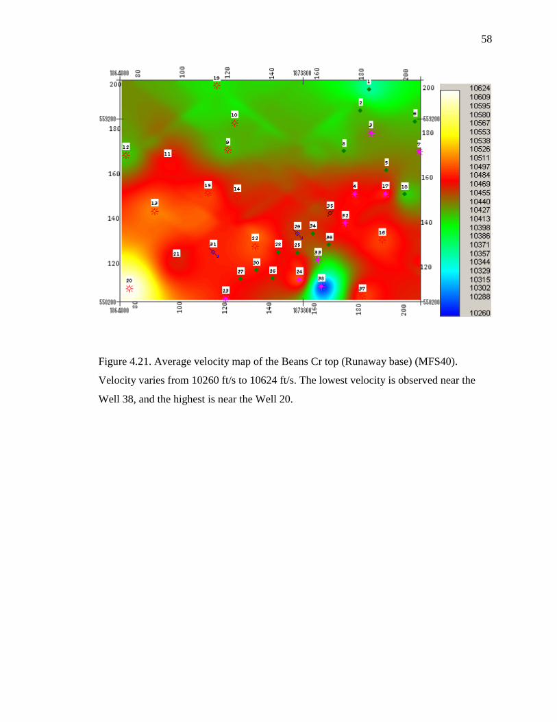
Figure 4.21. Average velocity map of the Beans Cr top (Runaway base) (MFS40).
Velocity varies from 10260 ft/s to 10624 ft/s. The lowest velocity is observed near the
Well 38, and the highest is near the Well 20.
Page 76
59
Figure 4.22. Average velocity map of the Vineyard (MFS20). Velocity varies from 10406
ft/s to 10709 ft/s. The lowest velocity is observed near the Well 38, and the highest is
near the Well 20.
Page 77
60
Figure 4.23. Average velocity map of the Wade top (Vineyard base) (MFS10). Velocity
varies from 10392 ft/s to 10742 ft/s. The lowest velocity is observed near the Well 38,
and the highest is near the Well 12.
Page 78
61
4.5.3. Depth Map. The structure maps obtained from the seismic data are in time.
In order to provide a good visualization to the structural features of horizons and wells,
time-depth conversion processing is needed. Using the average velocities, the depth map
for the targeted horizons are shown in Figures 4.24, 4.25, 4.26, 4.27, 4.28 and 4.29,
respectively, for the Caddo top (MFS90), Davis top (MFS70), Runaway top (MFS53),
Beans Creek top (MFS40), Vineyard top (MFS20), and Wade top (MFS10). In addition, a
3D view of all the generated depth maps for the targeted formations in Atoka is shown in
Figure 4.30. In Figure 4.31, the Runaway Formation, bounded by MFS53 and MFS40, is
visualized by the 3D depth view. The 3D depth view of the Vineyard Formation, bounded
by MFS20 and MFS10, is visualized in Figure 4.32. These 3D views show the effect of
the karst collapse features on the structure of the formations. The anticlines traps can be
identified.
Page 79
62
Figure 4.24. The Caddo (MFS90) depth map in TVD from the seismic datum (ft)
showing that the layer is dipping toward north. Depth varies from 4453 ft to 4749 ft.
Anticline is observable near the Well 38.
Page 80
63
Figure 4.25. The Davis (MFS70) depth map in TVD from the seismic datum (ft) showing
that the layer is dipping toward north. Depth varies from 4774 ft to 5137 ft. Anticline are
visuable near the Wells 26, 31, and 38. Karst collapse features are observed near the
Wells 6 and 18.
Page 81
64
Figure 4.26. The Runaway (MFS53) depth map in TVD from the seismic datum (ft)
showing that the layer is dipping toward north-east. Depth varies from 5053 ft to 5365 ft.
Anticline are observable near the Wells 2, 15 and 38. Karst collapse features are observed
near the Wells 6, 8, 18, and 35.
Page 82
65
Figure 4.27. The Bean Cr (MFS40) depth map in TVD from the seismic datum (ft)
showing that the layer is dipping toward north-east. Depth varies from 5130 ft to 5474 ft.
Anticline are observable near the Wells 15, 21 and 38. Karst collapse features are
observed near the Wells 6, 8, 18, and 35.
Page 83
66
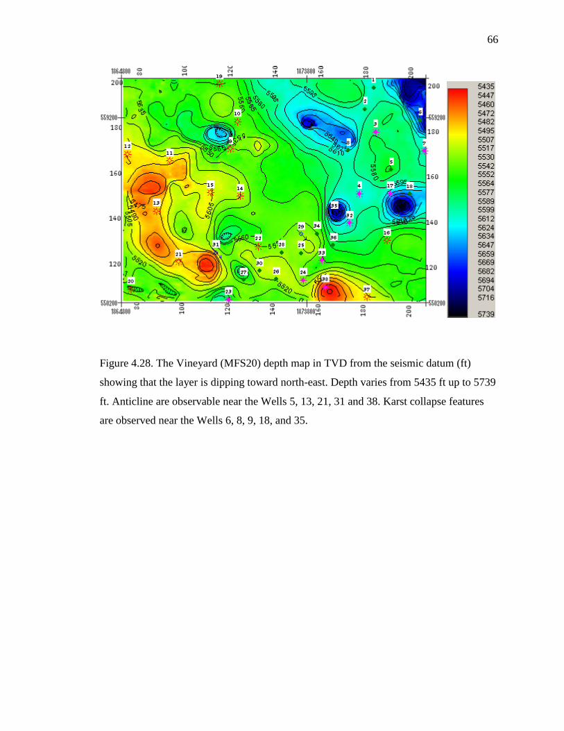
Figure 4.28. The Vineyard (MFS20) depth map in TVD from the seismic datum (ft)
showing that the layer is dipping toward north-east. Depth varies from 5435 ft up to 5739
ft. Anticline are observable near the Wells 5, 13, 21, 31 and 38. Karst collapse features
are observed near the Wells 6, 8, 9, 18, and 35.
Page 84
67
Figure 4.29. The Wade (MFS10) depth map in TVD from the seismic datum (ft) showing
that the layer is dipping toward east. Depth varies from 5560 ft up to 5905 ft. Anticline
are observable near the Wells 2, 5, 11, 12, 13, 31 and 38. Karst collapse features are
observed near the Wells 6, 8, 9, 18, and 35.
Page 85
68
Figure 4.30. 3D structure depth view for all the targeted formations. Depth is in TVD
from the seismic datum (ft). Form the top: the Caddo top (MFS90), Davis top (MFS70),
Runaway top (MFS53), Beans Creek top (MFS40), Vineyard top (MFS20), and Wade top
(MFS10). The Bend Conglomerate interval can be represented by the thickness of 1200 ft
from the top of the Caddo to the bottom of the Wade. Some karst collapse features are
found in the north-east. The dipping directions of the structure change from the northeast
dipping at the top to the east dipping at the bottom.
Caddo
Davis
Runaway
Beans Cr
Vineyard
Wade
Page 86
69
Figure 4.31. 3D depth structure view of the Runaway Formation top (MFS53) and base
(MFS40). Some karst collapse features are in the northern-east part. Anticline is at south.
Depth is in TVD from the seismic datum (ft).
Runaway Formation Top: MFS53
Base: MFS40
N
Page 87
70
Figure 4.32. 3D depth structure view of the Vineyard Formation top (MFS20) and base
(MFS10). Karst collapse features are located in the northern-east and the northern west.
Anticlines are located in the west and the south. Depth is in TVD from the seismic datum
(ft).
Top: MFS20
Base: MFS10
Vineyard Formation
N
Page 88
71
4.5.4. Time to Depth Conversion. Seismic data are provided in time domain.
However, it is more realistic to view the seismic data in depth, which gives better
understanding of the geological features.
By correlating depth grids with the time structure grids, the conversions for the
seismic data from time to depth are conducted using the SMT Kingdom Suite Software.
Figure 4.33 shows a vertical seismic section in depth after conversion.
Page 89
72
Figure 4.33. Vertical seismic section in depth. The horizons of the targeted formations are
shown as follows: Caddo (blue), Davis (Pink) Runaway (yellow) Beans Cr (light brown)
Vineyard (green), and Wade (dark green). Depth is subsea in ft. Color bar shows the
amplitude variation values.
Page 90
73
5. STRATIGRAPHIC INTERPRETATION
Stratigraphic interpretation of the Boonsville field is challenging, because there
are many karst collapse features, which randomly cut the targeted formations. This
affects the continuity of the targeted formations. The fluvial to deltaic depositional
environment is characterized by deltas, sand bodies, channel, and point bars, which are
shown as discontinuous thin sequences formed as described in Figure 2.9. In order to
better understanding the stratigraphic features in the area, the following interpretations
are conducted.
5.1. HORIZON SLICE
Horizon slice is useful in stratigraphic interpretations. It can help identifying the
features over the mapped formation. Horizon slices computed from the tracked horizons
are illustrated in Figures 5.1, 5.2, 5.3, and 5.4.
Page 91
74
Figure 5.1. The Runaway top (MFS53) horizon slice indicating a channel by the high
amplitudes.
Page 92
75
Figure 5.2. Horizon slice for the Beans Cr (MFS40), base of Vineyard, indicating a
channel flowing toward southwest.
Page 93
76
Figure 5.3. Top Vineyard (MFS20) horizon slice showing a channel indicated by the high
amplitudes from the south to north. The Karst collapse features are observed around the
Well 25. Very high amplitudes near the Well 16 suggest a Direct Hydrocarbon Indicator
(DHI) bright spot.
Page 94
77
Figure 5.4. Horizon slice of the Wade (MFS10), the Vineyard Base showing the effect of
karst collapse features at the base of the Bend Conglomerate near the Wells 6, 8, 18, 27,
33, and 35. The high amplitude feature that elongates north-south is suggested to be a
fluvial dominated mouth bar.
Page 95
78
5.2. ISOPACH MAP
Once the horizons are tracked, the isopach maps can be constructed if the interval
velocity information is available. Isopach maps show the thickness variations of the
targeted formations in the study area.
5.2.1. Interval Velocity Map. Interval velocity is the seismic velocity over a
specific interval of rock or strata. It can be expressed mathematically by the following
equation:
(3)
Where Vint is the interval velocity, D1 is the depth to the upper reflector, D2 is the
depth to the lower reflector, T1 is the two way travel time to the upper reflector, and T2 is
the two way travel time to the lower reflector (Figure 5.5)
Figures 5.5. Illustration showing the method to compute the parameters from the well
formation tops and the seismic time structure in order to calculate the interval velocity.
Page 96
79
Using the Kingdom Suite Software, the interval velocity map is generated once
the time structure is obtained for both the upper horizon and the lower horizon of the
targeted formation. For each well, the formation tops are needed to calculate the velocity
interval. The interval velocity values from each well can be gridded to generate an
interval velocity map for a specific formation. The gridding method used is the gradient
projection, which is similar to the method used in the structural interpretation maps.
Figures 5.6 and 5.7 show the interval velocity maps generated for the Runaway and
Vineyard Formations, respectively.
Figures 5.6. The Runaway Formation interval velocity map. The lowest interval velocity
is observed near the Wells 1 and 19, and the highest is near the Wells 17 and 20. The
interval velocity is decreasing toward north.
Page 97
80
Figures 5.7. The Vineyard Formation interval velocity map. The lowest interval velocity
is observed near the Well 2, and the highest is near the Wells 12 and 19.
Page 98
81
5.2.2. Isopach Map. Isopach map shows the variation in thickness of the targeted
formation, which can be used for many geological and petrophysical interpretations,
especially for studying the stratigraphic thickness and the depositional environment of
formation. In addition, it is used for the reservoir estimation and obtaining petrophysical
parameters such as the Net to Gross Ratio (NGR). In this study, isopach maps are
generated for the Runaway and Vineyard Formations (Figures 5.8 and 5.9).
Figure 5.8. The Runaway Formation isopach map showing the formation thickness
varying from 22 ft to 183 ft. The formation becomes thinner toward northwest.
Page 99
82
Figure 5.9. The Vineyard Formation isopach map showing the formation thickness
varying from 34 ft to 230 ft.
Page 100
83
5.3. WELL LOG CORRELATION
Well logs are used to interpret the stratigraphic features in the study area. Gamma
Ray (GR) and Spontaneous Potential (SP) are utilized to identify the lithology (Asquith
and Kryqowski, 2004). Resistivity logs (Rt) helps identify the type of fluids in the rock
voids (Asquith and Kryqowski, 2004). GR and Rt logs provided are shown in the base
map for the Runaway and Vineyard Formations, respectively (Figures 5.10 and 5.11).
Figure 5.12 shows correlations between logs of the Wells 1, 2, 3, 10, and 19 for
the Runaway Formation. Thick sand is presented in the Well 2. It represents a channel.
Figure 5.13 shows correlations between logs of the Wells 1, 2, 3, and 7 for the Runaway
Formation. In Figure 5.14, GR and Rt logs of the Well 2 are shown on the seismic section
for the Runaway Formation. In Figure 5.15, Gr and Rt logs of the Well 19 are shown on a
seismic section. A point bar truncation is observed in the Runaway Formation. A channel
near the Well 2 can be identified in Figure 5.16.
A cross correlation between logs of the Wells 16, 17, 27 and 37 for the Vineyard
Formation is shown in Figure 5.17. The logs from the Wells 16 and 37 indicate channel
fills in the upper of the Vineyard Formation. In Figure 5.18, logs of the Wells 16 and 24
are shown on a seismic section. A point bar truncation is identified in the Vineyard
Formation near the Well 24.
Page 101
84
Figure 5.10. GR and Rt logs showing in the basemap for the Runaway Formation.
Page 102
85
Figure 5.11. GR and Rt logs showing in the basemap for the Vineyard Formation.
Page 103
86
Figure 5.12.Well log correlation for the Runaway Formation. a) Horizon slice of the
Runaway top showing a channel and the arbitrary line location from the Well 1 to the
Well 19. b) The Runaway Formation bounded between MFS53 and MFS40 along the
cross section for well log correlation. Channel sand body is noticed in the Well 2. The
logs in the Wells 10 and 19 indicate shale dominating.
a)
b)
Page 104
87
Figure 5.13. Well log correlation for the Runaway Formation a) Horizon slice of the
Runaway top showing the arbitrary line location from the Wells 1 to the Well 7. b) The
Runaway Formation bounded between MFS53 and MFS40 along the cross section for
well log correlation. Channel sand body is noticed in the Well 2. The logs in the Well 7
show dominate point bar.
a)
b)
Page 105
88
Figure 5.14. SP-Rt log from the Well 2 showing in the seismic section for the Runaway
Formation. A channel is identified in both seismic sections in time (top) and in depth
(bottom). Depth is subsea (ft).
Page 106
89
Figure 5.15. GR (green) and Rt (blue) logs from the Well 19 showing in the seismic
section of crossline 199. A point bar truncation is observed in the Runaway Formation.
Page 107
90
Figure 5.16. Rt logs for the Wells 2, 4 and 37 plotted in the seismic section. A channel fill
is located near the Well 2 in the Runaway Formation.
Page 108
91
Figure 5.17. Well log correlation for the Vineyard Formation. a) Horizon slice of the
Vineyard top showing the arbitrary line location from the Well 17 to the Well 24. b) The
Vineyard Formation bounded between MFS20 and MFS10 along the cross section for the
well log correlation. Channel sand body is noticed in the Wells 16 and 37. The logs in the
Well 9 show dominate point bar.
a)
b)
Page 109
92
Figure 5.18. Well logs placed in the vertical seismic section for the Vineyard Formation.
a) Horizon slice of the Vineyard top showing the arbitrary line location. b) The seismic
section showing SP-Rt logs for the Well 16 indicates a channel fill, and the GR-Rt logs
for the Well 24 indicates a point bar truncation in the Vineyard Formation bounded by
MFS20 (top) and MFS10 (base).
a)
b)
Page 110
93
6. RESERVOIR ESTIMATION
6.1. INTRODUCTION
Reservoir estimation is important for many aspects. The information obtained is
used to identify prospects. It is also valuable for production and development for the
hydrocarbon reservoir fields. Various data such as well data, logs, cuttings, core data,
core plugs, production tests, and petrophysical data can be processed, analyzed and
interpreted to improve the well production, or help identifying prospects.
The reservoir properties are extracted from the seismic data in the target zones.
They are used for attribute measurements of the geophysical and geological data, which
are used in many different interpretation aspects such as stratigraphic interpretation,
structural interpretation, and reservoir evaluation.
6.2. ROOT-MEAN SQUARE AMPLITUDE
The depth difference between a top layer and a bottom layer of a reservoir is the
isopach. The isopach can provide the volume of the reservoir zone of the targeted
formations. The formation zones of the Runaway and Vineyard Formations have been
identified in this study using the depth maps and the isopach maps illustrated in Chapters
5. A top plane indicates the starting point of the volumetric calculation. A bottom plane
defines the volumetric polygon areas that describe the xy extent of the volumetric
calculation.
The Root-Mean-Square (RMS) amplitude is a post stack amplitude attribute.
Mathematically, it is calculated by using the square root of the sum of squared amplitudes
divided by the number of samples within the specified window. It is an effective attribute
Page 111
94
that helps determining hydrocarbon prospects. In fact, it enhances hydrocarbon bright
spots and can be used as a Direct Hydrocarbon Indicator (DHI). The RMS amplitude map
for the Runaway Formation bounded by MFS53 and MFS40 is illustrated in Figure 6.1.
In Figure 6.2, the RMS amplitude map is illustrated for the Vineyard Formation bounded
by MFS20 and MFS10.
Figure 6.1. RMS amplitude map of the Runaway Formation with the depth structural
contour of the Runaway top. Black shows bright spots near the Well 2. The suggested
prospect area is shaded by the red lines.
Page 112
95
Figure 6.2. RMS amplitude map of the Vineyard Formation with the depth structural
contour of the Vineyard top. Black shows bright spots near the Wells 16, 37, and 38. The
suggested prospect area is shaded by the blue lines.
Page 113
96
6.3. PETROPHYSICAL ANALYSIS
Petrophysical analyses are conducted by integrating the previous interpretations
and well log analysis to obtain the reservoir properties. Figure 6.3 shows the logs
computed from the Rt log of the Well 2. Figure 3.1 shows a list of wells with resistivity
logs while many do not have the bulk density logs (RHOB), and velocity or sonic logs
(DLT). In this study, some petrophysical parameters are obtained from analyzing the
well logs. The reservoir properties calculated are shown below in Table 6.1 for the
Runway Formation and in Table 6.2 for the Vineyard Formation.
Table 6.1. Calculated reservoir properties from the Runaway Formation
Well# Well Gross
(ft) Net (ft) NGR Porosity Sw K (md) HPV (ft)
2 ASHEB3 69.54 67.00 0.96 0.08 0.46 0.05 2.92
8 ASHEC6 78 67.5 0.870 0.17 0.32 0.01 7.7
12 BY11 75 7 0.090 0.09 0.4 0.12 0.37
13 BY13 72 43.5 0.600 0.18 0.4 0.36 4.96
14 BY15 70 32 0.460 0.19 0.36 0.5 4.27
15 BY18D 73 35 0.480 0.12 0.32 0.1 3.05
19 CY9 53 25.5 0.480 0.15 0.44 0.11 2.12
Table 6.2. Calculated reservoir properties from the Vineyard Formation
Well# Well Gross
(ft) Net (ft) NGR Porosity Sw K (md) HPV (ft)
8 ASHEC6 135.5 108.5 0.8 0.15 0.35 0.01 10.66
12 BY11 117 16.5 0.14 0.08 0.34 0.23 0.99
13 BY13 120 24 0.2 0.11 0.33 0.22 1.83
14 BY15 116 25 0.22 0.12 0.24 0.17 2.4
19 CY9 112.1 39 0.35 0.13 0.29 2.2 3.61
24 IGY9A 132.6 94 0.71 0.16 0.34 0.02 9.82
Page 114
97
Figure 6.3. Logs generated from the Rt (RILD) log of the Well 2.
Page 115
98
The petrophysical parameters describe the reservoir properties and can be used for
the volumetric calculation. They are either collected from the Boonsville field data set, or
calculated using the SMT Kingdom suite. Following are a list of these reservoir
properties:
6.3.1. Volume of Shale (Vsh). The Vsh is an important parameter in
petrophysical analysis. It indicates the lithology of the rock. SP log was used to calculate
Vsh. Equation (4) below expresses the relationship between Vsh and the SP log (Asquith
and Kryqowski, 2004).
Vsh = (SP – SPcln) / (SPsh – SPcln) (4)
Where SP is the spontaneous potential (in millivolts), SPcln is the spontaneous
potential within clean interval which is estimated 7% cut off (in millivolts), and SPsh is
the spontaneous potential within shale interval estimated 10% cut off (in millivolts)
(Figure 6.4). Vsh logs generated are shown in Figures 6.3, 6.5 and 6.6.
Page 116
99
Well 2 Well 16
For Well 2
For Well 16
Figure 6.4. SP logs for the Wells 2 and 16 showing examples for calculating the SPcln by
7% cut off and calculating SPsh by 10% cut off.
Page 117
100
6.3.2. Net to Gross Ratio (NGR). NGR is the ratio between Gross and Net pays.
Gross pay is the thickness between the upper and lower layers. Net pay is the total
thickness of zones satisfying conditions of productive formations. NGR is useful to
calculate the pore volume or the net volume (PV). PV is the total volume of the effective
pores in the reservoir (Djebbar and Erle, 2004).
6.3.3. Porosity (Φ). Porosity expresses the fraction of the rock pore volume (PV)
over the bulk volume (BV). The most important type of porosity is the effective porosity
(Φe) which measures the connectivity of voids of the rock (Figures 6.5 and 6.6). The
density logs are useful for porosity calculation. First, velocity logs were estimated using
the Faust relationship (Faust, 1953):
Velocity = C (D Rt) 1/6
(4)
Where C = 1948, a constant for English unite. Rt is the resistivity, and D is the
corresponding depth. Then, density logs (RHOB) are generated using the velocity logs
(Gardner, 1974):
RHOB = C1 Velocity0.25
(5)
Where C1 = 0.2295, a constant depending on the rock type. Density porosity
(PHID) can be calculated (Asquith and Kryqowski, 2004):
Page 118
101
PHID = (RHOMA – RHOB) / (RHOMA – RHOF) (6)
Where fluid density (RHOF) can be assumed as 1.0, and the matrix density
(RHOMA) is 2.65 for sand. If density and neutron logs are available, the effective
porosity log (PHIE) can be calculated (Asquith and Kryqowski, 2004). The relation is
expressed as following:
PHIE = [(PHID + PHIN) / 2.0] x (1 – Vsh) (7)
Where PHID is the density porosity (in decimals), PHIN is the neutron porosity
(in decimals), and Vsh is the shale volume (in decimals). In addition, porosity can be
calculated from the sonic log (DLT) (Asquith and Kryqowski, 2004). It is called sonic
porosity (PHIS) and is calculated in equation (8) below:
PHIS = [(DLT – DLTM) / (DLTF – DLTM)] x C (8)
Where DLT is the sonic travel time (in µs/ft), DLTM is the sonic travel time of
the matrix which is 52.6 µs/ft for consolidated sandstone, DLTF is the sonic travel time
of the fluid 190 µs/ft, and C is a constant, which is 0.7 for gas and 0.9 for oil. PHIE logs
generated are shown in Figures 6.3, 6.5 and 6.6.
Page 119
102
6.3.4. Water Saturation (Sw). Sw is a ratio of the pore volume filled with water
over the bulk volume. It can be obtained from the resistivity logs (Asquith and
Kryqowski, 2004). Sw is expressed mathematically by the Archie equation:
(9)
Where Rw is the resistivity of the formation water assumed to be 0.02 ohm-meter,
Rt is the value from the resistivity log in ohm. A is the tortuosity factor which is 1, m is
the cementation exponent which is 2, n is a constant varying from 1.8 – 2.5, commonly, it
is 2.0. Sw generated is shown in Figures 6.3, 6.5 and 6.6.
6.3.5. Permeability (K). Permeability is the movement ability of fluids within the
formation. The permeability log can be derived from the water saturation and the porosity
using the Wyllie and Rose (1950) method (Asquith and Kryqowski, 2004):
(10)
Where K is the permeability in millidarcies (md), C is 250 for medium gravity
oils or 79 for dry gas, Φ is the porosity, and Sw-irr is the water saturation of a zone at
irreducible water saturation.
Page 120
103
6.3.6. Gas Formation Factor (Bg). Gas formation factor is the volume of gas in
the reservoir occupied by a standard cubic foot of gas at the surface, which equals the
volume at reservoir conditions per volume at standard conditions in SCF/ft3 (Djebbar and
Erle, 2004).
(11)
Where p is the reservoir pressure in psi which can be estimated to be 1200 psi for
the Boonsville field, Z is the Z factor or gas deviation factor (also known as
compressibility factor estimated to be 0.78), T is the absolute temperature which is 460 +
reservoir temperature in oF (150+460) = 610
o. The calculated gas formation factor (Bg) is
89.2 SCF/ft3 for the Boonsville field.
Page 121
104
Figure 6.5. Well 2 logs generated from the petrophysical analysis showing the shale
volume (Vsh) and effective porosity (PHIE). For the Runway Formation (between
MFS53 and MFS40), the logs show good PHIE and unmoved hydrocarbons indicating a
potential reserve near the Well 2.
Page 122
105
Figure 6.6. Well 16 logs generated from the petrophysical analysis showing the shale
volume (Vsh) and effective porosity (PHIE). For the Vineyard Formation (between
MFS20 and MFS10), the logs show good PHIE and unmoved hydrocarbons indicating a
potential reserve near the Well 16.
Page 123
106
6.4. VOLUMATRIC CALCULATION
The volumetric analysis provides an estimation of the hydrocarbon reserve in the
targeted formation. To get a good understanding of the hydrocarbon potential of the Bend
Conglomerate, volumetric prospect are calculated by obtaining the Recoverable Original
Gas in-Place (ROGIP) in million cubic feet (MMCF) in the following equation (Djebbar
and Erle, 2004):
ROGIP = 43,560 NV Φe (1-Sw) Bg x RF (11)
Where NV is the net volume, Φe is the effective porosity represented by PHIE,
Sw is the water saturation, Bg is the gas formation factor, and RF is the recovery factor
which is estimated to be 70% of the OGIP.
Both targeted formations, the Runaway and Vineyard, are potential reservoirs in
the Bend Conglomerate. RMS amplitude maps are generated for both formations to get
the best DHI bright spots and helps to identify the prospect area for both formations by
correlating with the seismic interpretation and petrophysical analysis. The prospect for
the Runaway and Vineyard Formations are indicated in Figures 6.2 and 6.3, respectively.
The isopach grid Lower Cut Off (LCO) assumed to be 35 ft for the Runaway Formation
and 40 ft for the Vineyard Formation. LOC is used to optimize the Gross Volume (GV)
of the areas identified in the polygons in Figures 6.2 and 6.3, to the estimated lower cut
off. Table 6.3 shows the calculated average reservoir properties and petrophysical
parameters used for the volumetric calculation.
Page 124
107
Table 6.3. Petrophysical parameters calculated for both Runaway and Vineyard
Formations
Formation Area
(Acre) LCO (ft) NGR PHIE Sw Bg
Runaway 184.269 35 0.497 0.157 0.259 89.20
Vineyard 382.697 40 0.40 0.12 0.32 89.20
In order to conduct the reservoir volumetric calculation, the estimated values for
the Gross Volume (GV), Net Volume (NV), Pore Volume (PV), Hydrocarbon Pore
Volume (HPV), OGIP, and ROGIP are needed. The volumetric calculation results are
shown in Table 6.4.
Table 6.4. The results of the volumetric calculations for both Runaway and Vineyard
Formations. mega (M) = 103, million (MM) = 10
6, billion (B) = 10
9
Formation Grid Area
(Acre)
GV (Acre ft)
NV (Acre ft)
PV (Acre Ft)
HPV (Acre ft)
OGIP (SCF)
ROGIP (SCF)
Runaway 183 6.69 M 3.28 M 491.60 363.78 1.41 B 989.44
MM
Vineyard 364 36.92 M 14.88 M 1.78 M 1.22 M 4.75 B 3.32 B
Page 125
108
7. CONCLUSION
This study is an integrated interpretation of the Boonsville field data set. The
results are summarized as following:
1. Structural interpretation yields valuable depth maps of the Caddo,
Runaway, and Vineyard. These structural depth maps help to identify traps
and anticlines over both Runaway and Vineyard Formations. The study
supported previous studies by suggesting that the Ellenberger karst
collapse features have critical role in hydrocarbon migration from the
Barnett Shale (source rock). The depth maps visualize the distribution of
these collapses in the Runaway and the Vineyard Formations. The
anticlines, that are close to the karst collapse features, are most likely high
potential reserve areas. In addition, the depth maps show that the
structures of the Bend are altering the dipping direction from dipping
toward east at the bottom to dipping toward north at the top of Caddo.
2. Stratigraphic interpretations are conducted by correlating the amplitude
maps, isopach maps, and well logs. The isopach maps were generated for
the Runway and Vineyard to show the thickness of the formations over the
area of study. The horizon slices suggest some channels, point bars, and a
mouth bar. Well log correlations were performed to verify the suggested
stratigraphic features.
Page 126
109
3. For the reservoir identification, RMS amplitude maps were generated for
the Runaway and Vineyard Formations. In addition, petrophysical
approaches were implemented to calculate the following reservoir
properties: the gross, net pay, NGR, water saturation, shale volume,
porosity, and gas formation factor. Integrated analysis of the depth maps,
isopach maps, horizon slices, well logs, and petrophysical data, gives a
good identification of the hydrocarbon spots for both targeted formations.
Finally, volumetric prospect calculations were conducted to estimate the
Recoverable Original Gas in-Place (ROGIP). The Runaway Formation
prospect shows a potential gas amount of 989.44 MMSCF. The Vineyard
Formation prospect shows a potential gas amount of 3.32 BSCF. These
values of ROGIP for both formations suggest that the Boonsville field
clastic formations of the Bend have a great potential for further production
and development.
Page 127
110
BIBLIOGRAPHY
Asquith, G., and D. Krygowski, 2004, Basic well log analysis, second edition, American
Association of Petroleum Geologist and Society of Exploration Geophysics,
Methods in Exploration, 244 p.
Carr, D. L., R. Y. Elphick, R. A. Johns, and L. S. Foulk, 1997, High-resolution reservoir
characterization of mid-continent sandstones using wireline resistivity imaging,
Boonsville (Bend Conglomerate) gas field, Fort Worth Basin, Texas, The Log
Analyst, v. 38, p. 54–70.
DeCelles, P. G., and K. A. Giles, 1996, Foreland basin systems, Basin Research, v. 8,
p. 105–123, doi: 10.1046/j.1365-2117.1996.01491.x.
Djebbar, T, and D. Erle, 2004, Petrophysics, second edition, Elsevier Inc, 890 p.
Faust, L. Y., 1953, A velocity function including lithological variation, Geophysics, v.
18, p. 271 – 88.
Galloway, W. E., 1989, Genetic stratigraphic sequences in basin analysis; I, Architecture
and genesis of flooding-surface bounded depositional units, AAPG Bulletin, v. 73/2,
p. 125-142.
Hardage, B. A., 1996, Boonsville 3-D data set, The Leading Edge, v. 15, no. 7, p. 835–
837, doi:10.1016/0191-8141 (85)90048-3.
Hardage, B. A., D. L. Carr, D. E. Lancaster, J. L. Simmons Jr., R. Y., Elphick, V. M.
Pendleton, and R. A. Johns, 1996a, 3-D seismic evidence of the effects of carbonate
karst collapse on overlying clastic stratigraphy and reservoir compartmentalization,
Geophysics, v. 61, p. 1336–1350, doi:10.1190/1.1444057.
Hardage, B. A., D. L. Carr, D. E. Lancaster, J. L. Simmons Jr., D. S. Hamilton, R. Y.
Elphick, K. L. Oliver, and R. A. Johns, 1996b, 3-D seismic imaging and seismic
attribute analysis of genetic sequences deposited in low-accommodation conditions,
Geophysics, v. 61, p. 1351–1362, doi:10.1190/1.1444058.
Hardage, B. A., J. L. Simmons Jr., D. E. Lancaster, R. Y. Elphick, R. D. Edson, and D. L.
Carr, 1996c, Boonsville 3-D seismic data set, Austin, Texas, University of Texas at
Austin, Bureau of Economic Geology, 40 p.
Page 128
111
Hentz, T. F., J. A. Kane, W. A. Ambrose, and E. C. Potter, 2006, Depositional facies,
reservoir distribution, and infield potential of the lower Atoka Group (Bend
Conglomerate) in Boonsville field, Fort Worth Basin, Texas: New look at an old
play (abs.), AAPG Annual Convention Abstracts Volume, v. 15, p. 46.
Hentz, T. F., E. C. Potter, and M. A. Adedeji, 2007, Reservoirscale depositional facies,
trends, and controls on sandstone distribution of the lower Atoka Group (“Bend
Conglomerate”), Fort Worth Basin, Texas (abs.), AAPG Annual Convention
Abstracts Volume, v. 16, p. 62.
Hill, R. J., D. M. Jarvie, J. Zumberge, M. Henry, and R. M. Pollastro, 2007, Oil and gas
geochemistry and petroleum systems of the Fort Worth Basin, AAPG Bulletin, v.
91, no. 4, p. 445–473, doi:10.1111/j.1365-3091.2004.00628.x.
IHS Energy, Inc., 2011, U.S. production and well history control databases, Englewood,
Colorado, CD-ROM.
Maharaj, V. T., and L. J. Wood, 2009, A quantitative paleogeographic study of the
fluvio-deltaic reservoirs in the Atoka interval, Fort Worth Basin, Texas, U.S.A.,
Gulf Coast Association of Geological Societies Transactions, v. 59, p. 495–509.
Martin, C. A., 1982, Petroleum geology of the Fort Worth Basin and Bend Arch area,
Dallas Geological Society, 442 p.
McDonnell, A., R. G. Loucks, and T. Dooley, 2007, Quantifying the origin and geometry
of circular sag structures in northern Fort Worth Basin, Texas: Paleocave collapse,
pull-apart fault systems, or hydrothermal alteration?, AAPG Bulletin, v. 91, p.
1295–1318, doi:10.1306/05170706086.
Pollastro, R. M., 2003, Geologic and production characteristics utilized in assessing the
Barnett Shale continuous (unconventional) gas accumulation, Barnett-Paleozoic
total petroleum system, Fort Worth Basin, Texas, Barnett Shale Symposium, Ellison
Miles Geotechnology Institute at Brookhaven College, Dallas, Texas, November
12–13, 2003, 6 p.
Pollastro, R. M., R. J. Hill, D. M. Jarvie, and C. Adams, 2004, Geologic and organic
geochemical framework of the Barnett-Paleozoic total petroleum system, Bend
arch–Fort Worth Basin, Texas (abs.), AAPG Annual Meeting Program, v. 13, p.
A113, CD-ROM.
Pollastro, R. M., D. M. Jarvie, R. J. Hill, and C. W. Adams, 2007, Geologic framework of
the Mississippian Barnett Shale, Barnett-Paleozoic total petroleum system, Bend
arch–Fort Worth Basin, Texas, AAPG Bulletin, v. 91, no. 4, p. 405–436,
doi:10.1306/10300606008.
Page 129
112
Thomas, J. D., and W. Texas, 2003, Integrating synsedimentary tectonics with sequence
stratigraphy to understand the development of the Fort Worth basin, AAPG Search
and Discovery, Article #90023
Thompson, D. M., 1982, Atoka Group (Lower to Middle Pennsylvanian), Fort Worth
Basin, Texas: Terrigenous depositional systems, diagenesis, and reservoir
distribution and quality, University of Texas at Austin, Bureau of Economic
Geology Report of Investigations, v. 125, 62 p.
Thompson, D. M., 1988, Fort Worth Basin, in L. L. Sloss, ed., Sedimentary cover—
North American Craton: U.S., Geological Society of America, Decade of North
American Geology Series, v. D-2, p. 347–352.
Walper, J. L., 1982, Plate tectonic evolution of the Fort Worth Basin, in C. A. Martin,
ed., Petroleum geology of the FortWorth Basin and Bend arch area, Dallas
Geological Society, p. 237–251.
Page 130
113
VITA
Name: Aamer Alhakeem
Nationality: Saudi
Phone: +1(573)578-9136, +966541424004
Email: [email protected]
In 2013, I received a Master of Science degree in Geology and Geophysics at
Missouri University of Science and Technology (MST). In 2007, I completed B.S.
Degree in Geophysics from King Fahd University of Petroleum and Minerals (KFUPM).
During my Master degree, I have been doing a thesis research of 3D Seismic
Interpretation of the Boonsville field using Kingdom Suite Software. At KFUPM, I was
elected president of the Earth Science Student Committee. As a geosciences committee,
we participated in many activities related to different fields such as, Geology,
Geophysics, Environmental Sciences and Petroleum Engineering
My practical experience involved joining EniRepSa Gas Ltd. (Eni-50%, Repsol-
30%, Aramco-20%). I worked in EniRepSa as Jr. Drilling Engineer after spending six
weeks in ENI Indonesia earning drilling engineering courses. Moreover, I joined Saudi
Aramco for summer training program, where I was exposed to the technical work
environment of Geophysics and Geology.