3rd Middle East Turbomachinery Symposium (METS III) 15-18...

Copyright© 2015 by Turbomachinery Laboratory, Texas A&M Engineering Experiment Station

DEVELOPMENT AND DESIGN OF ANTISURGE AND PERFORMANCE CONTROL SYSTEMS

FOR CENTRIFUGAL COMPRESSORS

Saul Mirsky, PE Chief Technology Officer

Compressor Controls Corporation

Des Moines, IA, USA

Wayne Jacobson

Global Technology Manager


Des Moines, IA, USA

David Tiscornia, PE

Control Systems Engineer


Houston, TX, USA

Jeff McWhirter, PE Houston/Gulf Coast Sales Manager


Houston, TX, USA

Medhat Zaghloul

Regional Manager – Abu Dhabi


Al Reem Island, Abu Dhabi, UAE

Saul Mirsky, CCC’s Chief Technology

Officer, is the distinguished author of

numerous technical papers and esteemed

lecturer on turbomachinery control

solutions. Mr. Mirsky has been with CCC

since 1980 and is part of the Company’s

Leadership Team. In this position, he

serves as a technology consultant,

coordinating efforts throughout the

Company to ensure consistency in both

methodology and technology. In addition, he also analyzes and

devises strategies for turbomachinery control solutions. Mr.

Mirsky continuously researches technological control issues in

various industries and recommends product development

improvements to new and existing products. His work has

awarded him several patents in control methodology for

turbomachinery. Mr. Mirsky is a professional engineer and

holds a Master’s Degree in electrical engineering from

Polytechnical University in Riga, Latvia. Mr. Mirsky may be

reached through the Company website:

http://www.cccglobal.com/contact-us

Wayne Jacobson is CCC’s Global

Technology Manager in Des Moines, IA..

Wayne joined CCC in 1996 as a Systems

Engineer with a BS in Mechanical

Engineering from the University of

Wisconsin – Platteville. His

responsibilities include providing technical

guidance and support throughout the

organization,develop and enhance control

applications, maintain and improve standard engineering and

overseeing the overall technical development of engineering

staff.

Jeff McWhirter is the Houston/Gulf

Coast Manager for CCC. His extensive

experience with turbomachinery controls

encompasses many industries and

extends to LNG plants - implementing

both the APCI and COP processes,

refineries utilizing fluidized catalytic

cracking(FCCU) and power recovery,

NGL facilities, oil and gas production

facilities including separation, injection,

gas lift and sales gas, as well ammonia and ethylene plants.

Mr. McWhirter is a member of the working committee for the

new Machinery Protection System API 670 5th edition

specification and joint authored a patent entitled “Compressor-

Driver Power Limiting in Consideration of Antisurge Control”

in December 2012. Jeff received his B.S. degree in Mechanical

Engineering from Texas A&M University in 1980 and is a

member of the ASME

Medhat Zaghloul is CCC’s Regional

Technology Manager for the Europe,

Middle East and Africa regions with CCC,

based in the Abu Dhabi Office. Medhat

joined CCC in 1993 with over 35 years in

the oil and gas industry and 15-years

specific to instrumentation controls for the

petrochemical industry. He is responsible

for the development of technical solutions

and control applications, and providing

technical guidance and support. Mr. Zaghloul holds a B.Sc. in

Electrical Engineering from the Cairo Institute of Technology

in Egypt.

3rd Middle East Turbomachinery Symposium (METS III) 15-18 February 2015 | Doha, Qatar | mets.tamu.edu


David Tiscornia is a control systems

engineer with CCC. Throughout his 12

year tenure at CCC, David has held

various positions including software

development, project engineering, and

new technology development. An

accomplished lecturer and thought

leader, Mr. Tiscornia has written and

presented papers and articles on

turbomachinery control solutions at industry events around the

globe. David holds BS and MS degrees from Purdue University

and is a registered Professional Engineer in Iowa.

ABSTRACT

The development and design of control systems for

centrifugal and axial compressors is discussed and explanations

given to bring together features of control systems on varying

machine designs. Potential problems resulting from such

differences will be addressed and resolutions offered.

INTRODUCTION

Control systems for centrifugal and axial compressors

(below term Dynamic Compressors, or for simplicity:

Compressors) follow the same rules and reasoning as do control

systems for other plants, processes, machines, etc. At the same

time, the nature of Dynamic Compressors includes many

additional dissimilar properties that make it essential to pay

considerably more attention to the design of control systems for

these machines. It is tempting to design and implement these

control systems “by the book”, and many systems were and still

are being implemented that way. However, operation of many

control systems that are below average acceptability tell us that

at best these systems are wasting energy, and often, they may

be allowing damage to the machines that they are intended to

control and protect.

This Tutorial is intended to help the Mechanical, or Process

Engineer that understands issues associated with the design of

mechanical elements of the machine and, is familiar with the

processing of gas through the system, but does not have

sufficient experience with the design of control systems for

these machines. It is assumed further in the Tutorial that the

user of the Tutorial is familiar with multitude topics involving

Dynamic Compressors and their application in industrial

processes. The focus of the Tutorial is to explain the direction

that must be taken in the design of the control systems for

Dynamic Compressors as based upon many years of experience

from the author's company. This Tutorial stresses our

explanation of how to bring together features of the control

system regardless of varying machine designs, and at the same

time, how to keep track of distinctive potential problems that

result from differences between machines and processes that

make the design of these systems more demanding and

uncertain.

The proper control system for a complex object can be

designed only after achieving a solid understanding of the

object to be controlled, the Dynamic Compressor in this case.

What follows is a brief review of the important features of a

Dynamic Compressor as a controlled object.

DYNAMIC COMPRESSOR AS A CONTROLLED

OBJECT

The Dynamic Compressor is a machine that converts

mechanical energy of the driver (electric motor, steam or gas

turbine, etc.) into energy of the gas being processed. Operation

of the Dynamic Compressor can be well presented in the

Compressor Map (or, Compressor Performance Map). The

Compressor Map (Figure 1) shows operation of the compressor

in an X-Y plot in which the Volumetric Flow, QS is used as X-

axis, and the Compression Ratio, RC as Y-axis of the plot

(further below this map is referred to as the map in QS–RC

coordinates, the other, most useful for analysis compressor map

is plotted in QS–HP coordinates).

Figure 1. Qs – Rc Compressor Map with common lines

of resistance, speed, and change in each.

Many various coordinates can and are being used, and at

times must be also integrated into the analysis of the

compressor, but the QS–HP plot allows a number of advantages.

The QS–HP plot is used in a majority of cases as the de-facto

standard way of presenting machine performance, whereas the

QS–RC map is used when combined operation of the

compressor and the process is being reviewed. The

performance of the compressor is shown in the compressor map

for a set of constant speeds, making the Speed, N of the

compressor the 3rd

commonly seen coordinate of the map, while

the controlled process can be represented in the Compressor

Map as lines of resistance. Figure 1 shows a few lines of

constant resistance that are typical for compressor operation. In

its steady state, the operating point of the compressor is always

located at a point of intersection of the line of constant

resistance and the line of constant speed. As the process

resistance or the compressor speed changes, the operating point


follows with some delay and lag to the new point of

intersection (see Figure 1).

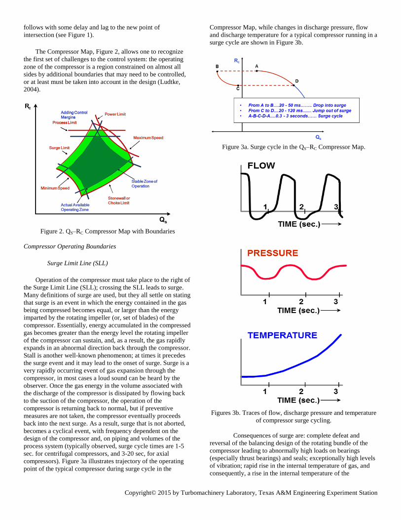
The Compressor Map, Figure 2, allows one to recognize

the first set of challenges to the control system: the operating

zone of the compressor is a region constrained on almost all

sides by additional boundaries that may need to be controlled,

or at least must be taken into account in the design (Ludtke,

2004).

Figure 2. QS–RC Compressor Map with Boundaries

Compressor Operating Boundaries

Surge Limit Line (SLL)

Operation of the compressor must take place to the right of

the Surge Limit Line (SLL); crossing the SLL leads to surge.

Many definitions of surge are used, but they all settle on stating

that surge is an event in which the energy contained in the gas

being compressed becomes equal, or larger than the energy

imparted by the rotating impeller (or, set of blades) of the

compressor. Essentially, energy accumulated in the compressed

gas becomes greater than the energy level the rotating impeller

of the compressor can sustain, and, as a result, the gas rapidly

expands in an abnormal direction back through the compressor.

Stall is another well-known phenomenon; at times it precedes

the surge event and it may lead to the onset of surge. Surge is a

very rapidly occurring event of gas expansion through the

compressor, in most cases a loud sound can be heard by the

observer. Once the gas energy in the volume associated with

the discharge of the compressor is dissipated by flowing back

to the suction of the compressor, the operation of the

compressor is returning back to normal, but if preventive

measures are not taken, the compressor eventually proceeds

back into the next surge. As a result, surge that is not aborted,

becomes a cyclical event, with frequency dependent on the

design of the compressor and, on piping and volumes of the

process system (typically observed, surge cycle times are 1-5

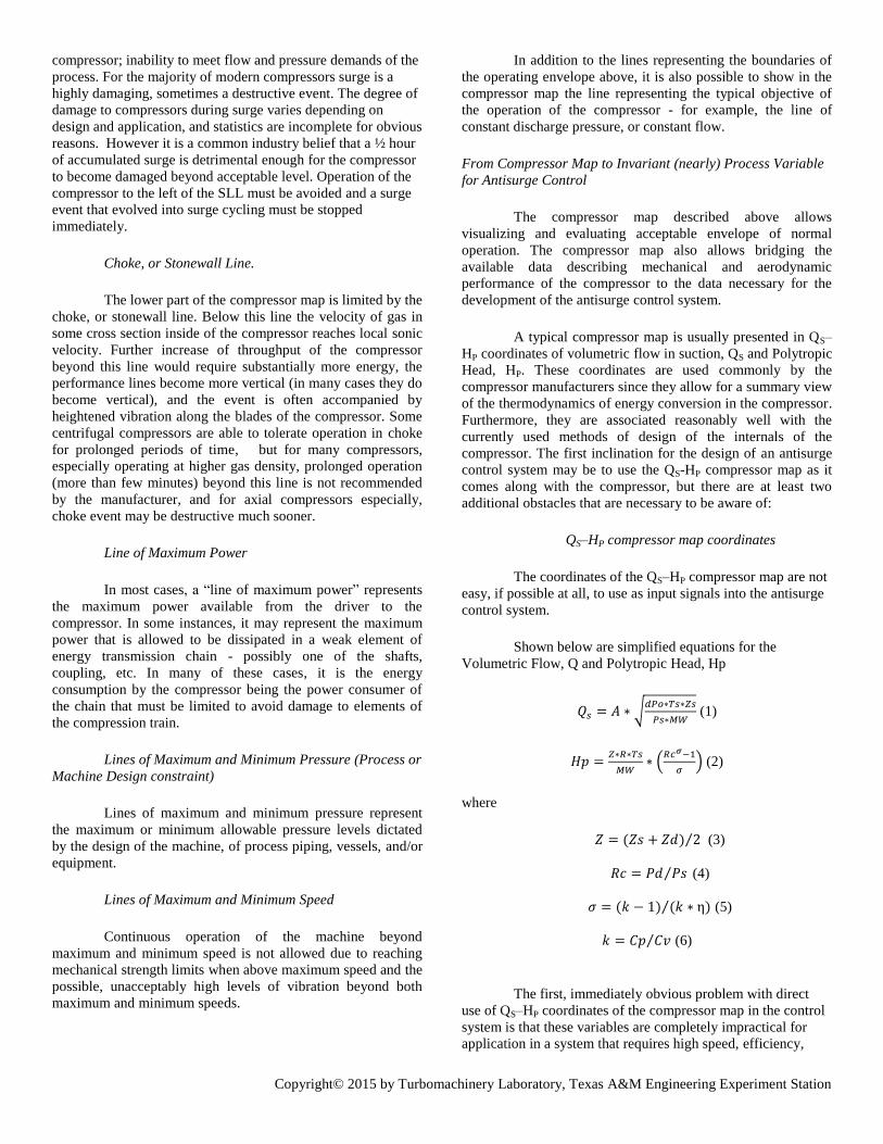
sec. for centrifugal compressors, and 3-20 sec, for axial compressors). Figure 3a illustrates trajectory of the operating

point of the typical compressor during surge cycle in the

Compressor Map, while changes in discharge pressure, flow

and discharge temperature for a typical compressor running in a

surge cycle are shown in Figure 3b.

Figure 3a. Surge cycle in the QS–RC Compressor Map.

Figures 3b. Traces of flow, discharge pressure and temperature

of compressor surge cycling.

Consequences of surge are: complete defeat and

reversal of the balancing design of the rotating bundle of the

compressor leading to abnormally high loads on bearings

(especially thrust bearings) and seals; exceptionally high levels

of vibration; rapid rise in the internal temperature of gas, and

consequently, a rise in the internal temperature of the


compressor; inability to meet flow and pressure demands of the

process. For the majority of modern compressors surge is a

highly damaging, sometimes a destructive event. The degree of

damage to compressors during surge varies depending on

design and application, and statistics are incomplete for obvious

reasons. However it is a common industry belief that a ½ hour

of accumulated surge is detrimental enough for the compressor

to become damaged beyond acceptable level. Operation of the

compressor to the left of the SLL must be avoided and a surge

event that evolved into surge cycling must be stopped

immediately.

Choke, or Stonewall Line.

The lower part of the compressor map is limited by the

choke, or stonewall line. Below this line the velocity of gas in

some cross section inside of the compressor reaches local sonic

velocity. Further increase of throughput of the compressor

beyond this line would require substantially more energy, the

performance lines become more vertical (in many cases they do

become vertical), and the event is often accompanied by

heightened vibration along the blades of the compressor. Some

centrifugal compressors are able to tolerate operation in choke

for prolonged periods of time, but for many compressors,

especially operating at higher gas density, prolonged operation

(more than few minutes) beyond this line is not recommended

by the manufacturer, and for axial compressors especially,

choke event may be destructive much sooner.

Line of Maximum Power

In most cases, a “line of maximum power” represents

the maximum power available from the driver to the

compressor. In some instances, it may represent the maximum

power that is allowed to be dissipated in a weak element of

energy transmission chain - possibly one of the shafts,

coupling, etc. In many of these cases, it is the energy

consumption by the compressor being the power consumer of

the chain that must be limited to avoid damage to elements of

the compression train.

Lines of Maximum and Minimum Pressure (Process or

Machine Design constraint)

Lines of maximum and minimum pressure represent

the maximum or minimum allowable pressure levels dictated

by the design of the machine, of process piping, vessels, and/or

equipment.

Lines of Maximum and Minimum Speed

Continuous operation of the machine beyond

maximum and minimum speed is not allowed due to reaching

mechanical strength limits when above maximum speed and the

possible, unacceptably high levels of vibration beyond both

maximum and minimum speeds.

In addition to the lines representing the boundaries of

the operating envelope above, it is also possible to show in the

compressor map the line representing the typical objective of

the operation of the compressor - for example, the line of

constant discharge pressure, or constant flow.

From Compressor Map to Invariant (nearly) Process Variable

for Antisurge Control

The compressor map described above allows

visualizing and evaluating acceptable envelope of normal

operation. The compressor map also allows bridging the

available data describing mechanical and aerodynamic

performance of the compressor to the data necessary for the

development of the antisurge control system.

A typical compressor map is usually presented in QS–

HP coordinates of volumetric flow in suction, QS and Polytropic

Head, HP. These coordinates are used commonly by the

compressor manufacturers since they allow for a summary view

of the thermodynamics of energy conversion in the compressor.

Furthermore, they are associated reasonably well with the

currently used methods of design of the internals of the

compressor. The first inclination for the design of an antisurge

control system may be to use the QS-HP compressor map as it

comes along with the compressor, but there are at least two

additional obstacles that are necessary to be aware of:

QS–HP compressor map coordinates

The coordinates of the QS–HP compressor map are not

easy, if possible at all, to use as input signals into the antisurge

control system.

Shown below are simplified equations for the

Volumetric Flow, Q and Polytropic Head, Hp

𝑄𝑠 = 𝐴 ∗ √𝑑𝑃𝑜∗𝑇𝑠∗𝑍𝑠

𝑃𝑠∗𝑀𝑊 (1)

𝐻𝑝 =𝑍∗𝑅∗𝑇𝑠

𝑀𝑊∗ (

𝑅𝑐𝜎−1

𝜎) (2)

where

𝑍 = (𝑍𝑠 + 𝑍𝑑) 2 ⁄ (3)

𝑅𝑐 = 𝑃𝑑 𝑃𝑠⁄ (4)

𝜎 = (𝑘 − 1) (𝑘 ∗ η)⁄ (5)

𝑘 = 𝐶𝑝 𝐶𝑣⁄ (6)

The first, immediately obvious problem with direct

use of QS–HP coordinates of the compressor map in the control

system is that these variables are completely impractical for

application in a system that requires high speed, efficiency,


accuracy, and reliability of input signals. Only the variables of

pressures and temperatures in the equations above can be

measured directly by use of available, reliable, and tested in

applications, industrial grade transmitters. Parameters of gas,

like Z, MW and k, can be measured by modern available

equipment. However accuracy, speed of response, reliability,

etc. of these measurements makes them unacceptable for

inclusion into a closed loop control system. The efficiency η of

the compressor (or compressor stage) of interest proves even

more elusive because its measurement would involve

comparing actual compression cycle with the idealized

compression cycle for the same gas.

Inferential Control System

In control systems the compressor antisurge control

system belongs under the classification of an “inferential

control system”, meaning that direct measurement of the

controlled variable - distance to surge in this case - is

unavailable, and that the controlled variable has to be inferred

from available measurements. There are two reasons for this.

First, the position of the SLL as presented in the compressor

map represents at best, the latest known position of the SLL

that may change in an unpredictable way with time and with

change in condition of the compressor. Second, position of

both the SLL and the operating point is influenced by changes

in gas composition, but as stated above, the use of gas

composition measurements for inclusion into the antisurge

control system should be avoided. There is not much that can

be done to improve measurability of the drift of the SLL as a

result of a changing condition of the compressor, unless some

newly invented method that allows a direct measurement of the

SLL is employed. It is possible, however, to deal with the

second problem.

For the operation of the antisurge control system, it is

necessary to measure and further express the distance between

present position of the operating point and the SLL of the

compressor. Varying position of the operating point can be

measured, but only in units of flow, pressure and temperature

without accounting for change in gas composition (see

explanation above); location of the SLL of the compressor is

not measurable directly during normal operation at all. Since

position of the SLL is not-measurable directly, it must be

inferred from the best data, previously obtained, and from

available flow, pressure and temperature measurements.

In practice this means that the SLL available for

control is representing our best knowledge at the time, and that

position of SLL must be periodically corrected to reflect the

change in its position with time and with compressor condition,

and that position of SLL also must be constantly reflecting

changes in gas parameters. Little can be done to improve the

ability of direct measurement of SLL position, therefore

continuous correction of the condition of the compressor drift is

hardly possible - but it is possible to work around continuous

correction for gas parameter changes.

One possible, but impractical, method for this would

be to obtain gas parameters necessary for the equations 1-6

above (in essence this would follow calculations that are

recommended and described in the ASME Testing Code PTC

10-1997). But since the use of measurements of gas parameters

is impractical, this method is not used for operation of the

antisurge control system.

Another alternative is to simplify the calculated

control inputs to the point where the calculations would not

contain variables that are difficult to obtain, but additionally

and most importantly, to perform this simplification in a way

that does not negatively affect accuracy of the result.

Substantial amount of studies of the topic of expressing control

inputs for a compressor in an invariant coordinate system can

be found in literature (Batson, 1996, Bloch, 1996).

Described below is the practical method performed in

a few steps of expressing compressor map in invariant

coordinates and establishing an appropriate control variable for

the antisurge control:

Expressing Compressor Map in Invariant Coordinates

Equations (1) and (2) representing the original

compressor map are a very good starting point to move to the

desired result. First the equation (1) is squared

𝑄𝑠2 = 𝐴2 ∗

𝑑𝑃𝑜∗𝑇𝑠∗𝑍𝑠

𝑃𝑠∗𝑀𝑊 (7),

Both equations (2) and (7) are then divided by a common factor 𝑇𝑠∗𝑍𝑠

𝑀𝑊 , which results in two new variables: Reduced Flow

Squared - 𝑞𝑠𝑟2 and Reduced Head - ℎ𝑝𝑟

𝑞𝑠𝑟2 =

𝑄𝑠2

𝑇𝑠∗𝑍𝑠

𝑀𝑊

=𝐴2∗

𝑑𝑃𝑜∗𝑇𝑠∗𝑍𝑠

𝑃𝑠∗𝑀𝑊𝑇𝑠∗𝑍𝑠

𝑀𝑊

=𝑑𝑃𝑜

𝑃𝑠 (8),

and

ℎ𝑝𝑟 =𝐻𝑝

𝑇𝑠∗𝑍𝑠

𝑀𝑊

=

𝑍∗𝑅∗𝑇𝑠

𝑀𝑊∗(

𝑅𝑐𝜎−1

𝜎)

𝑇𝑠∗𝑍𝑠

𝑀𝑊

= (𝑅𝑐𝜎−1

𝜎) (9)

Equations (8) and (9) omit constants, and an assumption is

made for the equation (9) that 𝑍 𝑍𝑠⁄ remains reasonably

constant within 1 to 2%, which is approximately correct within

operating range of many applications. For some applications

such as propane and high pressure carbon dioxide, 𝑍 𝑍𝑠⁄ can

vary 4% or more and further analysis must be performed.

Polytropic exponent σ in the equation (9) above can be

assumed constant if gas composition and gas parameters remain

reasonably constant within operating range of the compressor,

but it may be necessary to correct for gas composition changes

in some cases, typically when molecular weight varies more

than 10%.


Using the definition of polytropic process:

(𝑃𝑑 𝑃𝑠⁄ )σ = (𝑇𝑑 𝑇𝑠⁄ ) (10)

It is possible to calculate the polytropic exponent σ on

line by using only available pressure and temperature signals,

basically using the results of the compression process for

calculation.

𝜎 = log(𝑇𝑑 𝑇𝑠⁄ )/ log (𝑃𝑑 𝑃𝑠⁄ ) (11)

The calculated value of polytropic exponent σ can

then be used in equation (9) for more accurate representation of

gas composition changes. Applying the calculated value of σ

can lead to a more accurate definition of the SLL for most

hydrocarbon gas mixtures that are typically used in the

petrochemical industry. If the mixture of gases is such that the

ratio of specific heats k is not changing with the change in

molecular weight and compressibility resulting in σ being

relatively constant, using equation (11) may not provide any

additional benefit to the definition of the SLL.

The new variables, Reduced Flow Squared, 𝑞𝑠𝑟2 and

Reduced Head, ℎ𝑝𝑟, do not contain non-measurable variables

that change with gas composition changes. In addition, the

compressor map in these coordinates acquires property of

invariance to changes in gas parameters. A number of papers

were published on the topic of proper selection of invariant

coordinates for the needs of the antisurge controls. The ones

selected above are the best served, in the opinion of the

author’s Company. As may be seen on Figure 4, use of these

variables for the compressor maps representing operation of the

compressor with different gas compositions reduces the

multitude of SLL into one contiguous, compacted SLL that can

be implemented in the control system.

Figure 4. Reduction of the SLL in QS–HP coordinates

The derived above equations constitute a good basis

for a nearly invariant compressor map coordinate, but even so,

the designer of the antisurge control system must verify and

validate assumptions made along the way. A recommended

sequence is: once the implementation of the system is decided

upon and the SLL is expressed as invariant and acceptable to

the control system implementation, the designer needs to

perform back-calculations to prove that the resulting error does

not exceed acceptable level.

A word of warning is in order. Many other invariant

parameter systems can be derived (Batson, 1996), but there

does not seem to be any advantage of using a majority of them,

and many of these parameter systems do not meet the

requirement of a high speed response for the system, or do not

exhibit an adequate sensitivity to change of position of the

operating point. As will be shown later, the antisurge control

system must be able to operate with an overall reaction speed

that allows it to cope with the high speed of commencement of

surge, which means that the selected variables must be able to

change at a speed not lower than possible changes in actual

position of the operating point. The analysis in this Tutorial is

focused on flow being one of the most useful variables, with

expectations for speed of pressure signals being somewhat

slower, and only horsepower of the driver and rotating torque,

that may be able to meet our high speed requirements.

Some notes for design of the antisurge control systems

must be made in use of the resulting variables in equations (8),

(9) above:

As previously stated, accuracy of the resulting

calculations is limited largely in part to a residual error due to

the fact that 𝑍 𝑍𝑠⁄ may not remain constant throughout

operating range of the compressor.

Additionally, derivation of invariant coordinates is

based on what is termed as: accepting conditions of similarity

between different operating conditions for which various

idealizing assumptions are being made. In practice, when gas

conditions are changed in a wide range, the reduced coordinates

become less accurate due to a large number of unaccounted for

factors (ASME PTC 10-1987). For example, the compressor

maps represent well operation of the compressor if the

measurements are taken immediately in the compressor, but

actual instrumentation performing these measurements is

installed outside of the compressor with inevitable errors due to

losses which affect the final results.

Still, analysis of the implemented control systems

shows that for majority of cases, the derived coordinates

successfully reduce the multiple lines representing the complex

surface of surge boundary into a singular line that can be

expressed by using only simple, available measurements (see

Figure 4).

Distance to Surge in Compressor Map in Invariant Coordinates

The analysis above resulted in a pair of reduced X-Y

map coordinates allowing for all desired qualities. Here is our

resulting pair:

𝑞𝑠𝑟2 =

𝑑𝑃𝑜

𝑃𝑠 and ℎ𝑝𝑟 = (

𝑅𝑐𝜎−1

𝜎) (12)


The next step is to produce a singular control variable that can

be used for the antisurge control. Division of the two

coordinates of equation (12) allows calculating slope of the line

to the operating point in the compressor map, SlopeOPL

𝑆𝑙𝑜𝑝𝑒𝑂𝑃𝐿 = ℎ𝑝𝑟 𝑞𝑠𝑟2⁄ (13),

Likewise, division of the two coordinates of equation (12) for a

point along the SLL allows one to calculate slope of the line to

the surge point in the compressor map, SlopeSLL

𝑆𝑙𝑜𝑝𝑒𝑆𝐿𝐿 = ℎ𝑝𝑟𝑆 𝑞𝑠𝑟𝑆2⁄ (14)

Finally, we can define the distance to surge control variable, as

𝑆𝑆 = 𝑆𝑙𝑜𝑝𝑒𝑂𝑃𝐿 𝑆𝑙𝑜𝑝𝑒𝑆𝐿𝐿⁄ (15)

The new variable SS represents an angular measure of the

distance between the operating point and the SLL in the

compressor map with X-Y coordinates as defined by equations

(12). Since coordinates of the compressor map as per equation

(12) were invariant, the derived variable SS retains the property

of invariance, too.

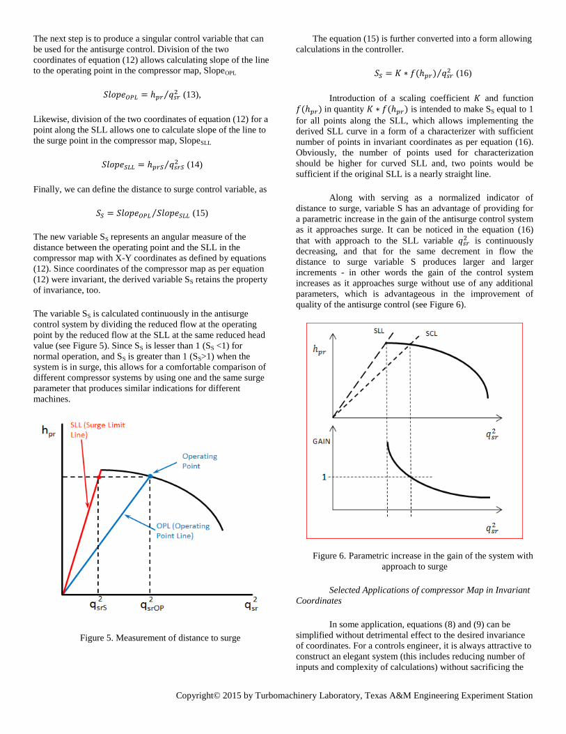
The variable SS is calculated continuously in the antisurge

control system by dividing the reduced flow at the operating

point by the reduced flow at the SLL at the same reduced head

value (see Figure 5). Since SS is lesser than 1 (SS <1) for

normal operation, and SS is greater than 1 (SS>1) when the

system is in surge, this allows for a comfortable comparison of

different compressor systems by using one and the same surge

parameter that produces similar indications for different

machines.

Figure 5. Measurement of distance to surge

The equation (15) is further converted into a form allowing

calculations in the controller.

𝑆𝑆 = 𝐾 ∗ 𝑓(ℎ𝑝𝑟) 𝑞𝑠𝑟2⁄ (16)

Introduction of a scaling coefficient 𝐾 and function

𝑓(ℎ𝑝𝑟) in quantity 𝐾 ∗ 𝑓(ℎ𝑝𝑟) is intended to make SS equal to 1

for all points along the SLL, which allows implementing the

derived SLL curve in a form of a characterizer with sufficient

number of points in invariant coordinates as per equation (16).

Obviously, the number of points used for characterization

should be higher for curved SLL and, two points would be

sufficient if the original SLL is a nearly straight line.

Along with serving as a normalized indicator of

distance to surge, variable S has an advantage of providing for

a parametric increase in the gain of the antisurge control system

as it approaches surge. It can be noticed in the equation (16)

that with approach to the SLL variable 𝑞𝑠𝑟2 is continuously

decreasing, and that for the same decrement in flow the

distance to surge variable S produces larger and larger

increments - in other words the gain of the control system

increases as it approaches surge without use of any additional

parameters, which is advantageous in the improvement of

quality of the antisurge control (see Figure 6).

Figure 6. Parametric increase in the gain of the system with

approach to surge

Selected Applications of compressor Map in Invariant

Coordinates

In some application, equations (8) and (9) can be

simplified without detrimental effect to the desired invariance

of coordinates. For a controls engineer, it is always attractive to

construct an elegant system (this includes reducing number of

inputs and complexity of calculations) without sacrificing the


quality of antisurge control. The examples below demonstrate

that there are cases that can be satisfied by simple solutions, but

for some cases the complexity of the solution is justified.

“Fan Law” compliant compressor

A “Fan Law” compliant compressor in constant gas

composition application may be adequately controlled by a

simple antisurge control system. A well-known Fan Law for

the compressors states that Q~N and HP~N2, and it is well

applicable to low head single stage compressors, hence the

name “Fan Law”. In our derived 𝑞𝑠𝑟2 –ℎ𝑝𝑟 coordinates, since

both coordinates are proportional to speed N, this means that

the SLL for this type of a compressor is represented by a

straight line out of origin of coordinates. Literature

(Staroselsky, 1979, Gresh 2001) shows that the straight line

assumption can be applied as long as the deviation from the Fan

Law is limited, and as long as the gas composition remains

constant.

If polytropic constant σ in equation (9) is considered

constant and if the values of Rc are not particularly high, the

equation (9) can be expressed, as

ℎ𝑝𝑟 = (𝑅𝑐𝜎−1

𝜎) 𝑅𝑐 − 1 =

𝑃𝑑

𝑃𝑠− 1 =

𝑃𝑑−𝑃𝑠

𝑃𝑠 (17),

and distance to surge S can be expressed as

𝑆 = 𝐾 ∗ 𝑓(ℎ𝑝𝑟) 𝑞𝑠𝑟2⁄ = 𝐾 ∗

(𝑃𝑑−𝑃𝑠)𝑃𝑠⁄

𝑑𝑃𝑜𝑃𝑠⁄

=𝑃𝑑−𝑃𝑠

𝑑𝑃𝑜=

𝑑𝑃𝑐

𝑑𝑃𝑜 (18)

An adequate antisurge control for this compressor may

need only two differential pressure transmitters!

To reiterate, the above solution works well only if the

gas composition is not changing, and if the head of the

compressor is low enough to result in a straight SLL. The exact

value of maximum Rc, for which this method is applicable,

differs dependent on the type of gas used, the head of the

compressor and the acceptable accuracy of implementation.

Compressor with Inlet Guide Vanes

Compressors with Inlet Guide Vanes may require IGV

position signal. A majority of axial compressors and some of

centrifugal ones are equipped by Inlet Guide Vanes (IGV) to

control throughput of the compressor.

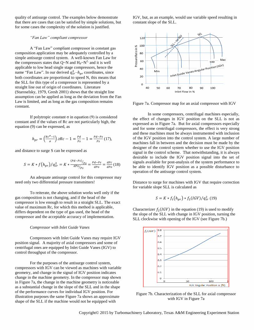
For the purposes of the antisurge control system,

compressors with IGV can be viewed as machines with variable

geometry, and change in the signal of IGV position indicates

change in the machine geometry. In the compressor map shown

in Figure 7a, the change in the machine geometry is noticeable

as a substantial change in the slope of the SLL and in the shape

of the performance curves for individual IGV position. For

illustration purposes the same Figure 7a shows an approximate

shape of the SLL if the machine would not be equipped with

IGV, but, as an example, would use variable speed resulting in

constant slope of the SLL.

Figure 7a. Compressor map for an axial compressor with IGV

In some compressors, centrifugal machines especially,

the effect of changes in IGV position on the SLL is not as

expressed as in Figure 7a. But for axial compressors especially

and for some centrifugal compressors, the effect is very strong

and these machines must be always instrumented with inclusion

of the IGV position into the control system. A large number of

machines fall in between and the decision must be made by the

designer of the control system whether to use the IGV position

signal in the control scheme. That notwithstanding, it is always

desirable to include the IGV position signal into the set of

signals available for post-analysis of the system performance to

be able to identify IGV position as a possible disturbance to

operation of the antisurge control system.

Distance to surge for machines with IGV that require correction

for variable slope SLL is calculated as

𝑆 = 𝐾 ∗ 𝑓1(ℎ𝑝𝑟) ∗ 𝑓2(𝐼𝐺𝑉) 𝑞𝑠𝑟2⁄ (19)

Characterizer 𝑓2(𝐼𝐺𝑉) in the equation (19) is used to modify

the slope of the SLL with change in IGV position, turning the

SLL clockwise with opening of the IGV (see Figure 7b.)

Figure 7b. Characterization of the SLL for axial compressor

with IGV in Figure 7a

Max


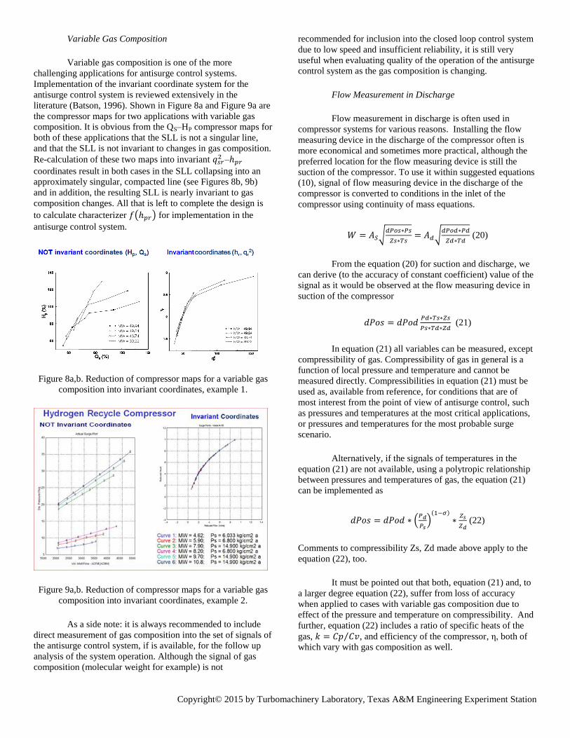
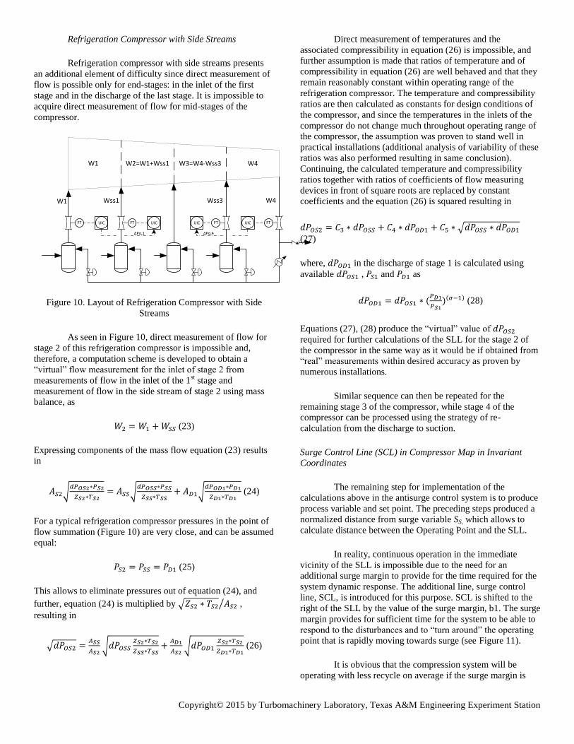
Variable Gas Composition

Variable gas composition is one of the more

challenging applications for antisurge control systems.

Implementation of the invariant coordinate system for the

antisurge control system is reviewed extensively in the

literature (Batson, 1996). Shown in Figure 8a and Figure 9a are

the compressor maps for two applications with variable gas

composition. It is obvious from the QS–HP compressor maps for

both of these applications that the SLL is not a singular line,

and that the SLL is not invariant to changes in gas composition.

Re-calculation of these two maps into invariant 𝑞𝑠𝑟2 –ℎ𝑝𝑟

coordinates result in both cases in the SLL collapsing into an

approximately singular, compacted line (see Figures 8b, 9b)

and in addition, the resulting SLL is nearly invariant to gas

composition changes. All that is left to complete the design is

to calculate characterizer 𝑓(ℎ𝑝𝑟) for implementation in the

antisurge control system.

Figure 8a,b. Reduction of compressor maps for a variable gas

composition into invariant coordinates, example 1.

Figure 9a,b. Reduction of compressor maps for a variable gas

composition into invariant coordinates, example 2.

As a side note: it is always recommended to include

direct measurement of gas composition into the set of signals of

the antisurge control system, if is available, for the follow up

analysis of the system operation. Although the signal of gas

composition (molecular weight for example) is not

recommended for inclusion into the closed loop control system

due to low speed and insufficient reliability, it is still very

useful when evaluating quality of the operation of the antisurge

control system as the gas composition is changing.

Flow Measurement in Discharge

Flow measurement in discharge is often used in

compressor systems for various reasons. Installing the flow

measuring device in the discharge of the compressor often is

more economical and sometimes more practical, although the

preferred location for the flow measuring device is still the

suction of the compressor. To use it within suggested equations

(10), signal of flow measuring device in the discharge of the

compressor is converted to conditions in the inlet of the

compressor using continuity of mass equations.

𝑊 = 𝐴𝑆√𝑑𝑃𝑜𝑠∗𝑃𝑠

𝑍𝑠∗𝑇𝑠= 𝐴𝑑√

𝑑𝑃𝑜𝑑∗𝑃𝑑

𝑍𝑑∗𝑇𝑑 (20)

From the equation (20) for suction and discharge, we

can derive (to the accuracy of constant coefficient) value of the

signal as it would be observed at the flow measuring device in

suction of the compressor

𝑑𝑃𝑜𝑠 = 𝑑𝑃𝑜𝑑𝑃𝑑∗𝑇𝑠∗𝑍𝑠

𝑃𝑠∗𝑇𝑑∗𝑍𝑑 (21)

In equation (21) all variables can be measured, except

compressibility of gas. Compressibility of gas in general is a

function of local pressure and temperature and cannot be

measured directly. Compressibilities in equation (21) must be

used as, available from reference, for conditions that are of

most interest from the point of view of antisurge control, such

as pressures and temperatures at the most critical applications,

or pressures and temperatures for the most probable surge

scenario.

Alternatively, if the signals of temperatures in the

equation (21) are not available, using a polytropic relationship

between pressures and temperatures of gas, the equation (21)

can be implemented as

𝑑𝑃𝑜𝑠 = 𝑑𝑃𝑜𝑑 ∗ (𝑃𝑑

𝑃𝑠)

(1−𝜎)

∗𝑍𝑠

𝑍𝑑 (22)

Comments to compressibility Zs, Zd made above apply to the

equation (22), too.

It must be pointed out that both, equation (21) and, to

a larger degree equation (22), suffer from loss of accuracy

when applied to cases with variable gas composition due to

effect of the pressure and temperature on compressibility. And

further, equation (22) includes a ratio of specific heats of the

gas, 𝑘 = 𝐶𝑝 𝐶𝑣⁄ , and efficiency of the compressor, η, both of

which vary with gas composition as well.


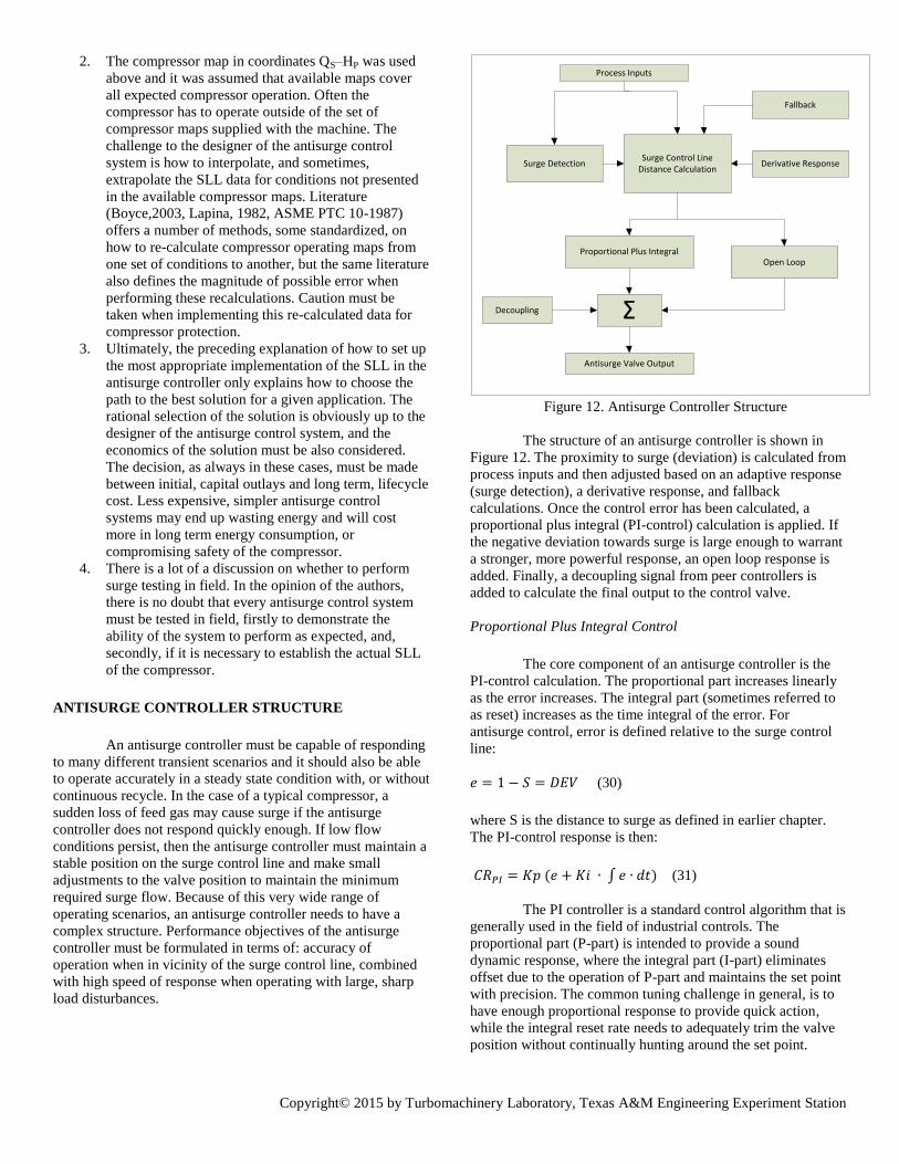
Refrigeration Compressor with Side Streams

Refrigeration compressor with side streams presents

an additional element of difficulty since direct measurement of

flow is possible only for end-stages: in the inlet of the first

stage and in the discharge of the last stage. It is impossible to

acquire direct measurement of flow for mid-stages of the

compressor.

FT FT FT FT

W1 W2=W1+Wss1 W3=W4-Wss3 W4

W1 Wss1 Wss3 W4

UIC UIC UIC UIC

ΔPo,4ΔPo,1

Figure 10. Layout of Refrigeration Compressor with Side

Streams

As seen in Figure 10, direct measurement of flow for

stage 2 of this refrigeration compressor is impossible and,

therefore, a computation scheme is developed to obtain a

“virtual” flow measurement for the inlet of stage 2 from

measurements of flow in the inlet of the 1st stage and

measurement of flow in the side stream of stage 2 using mass

balance, as

𝑊2 = 𝑊1 + 𝑊𝑆𝑆 (23)

Expressing components of the mass flow equation (23) results

in

𝐴𝑆2√𝑑𝑃𝑂𝑆2∗𝑃𝑆2

𝑍𝑆2∗𝑇𝑆2= 𝐴𝑆𝑆√

𝑑𝑃𝑂𝑆𝑆∗𝑃𝑆𝑆

𝑍𝑆𝑆∗𝑇𝑆𝑆+ 𝐴𝐷1√

𝑑𝑃𝑂𝐷1∗𝑃𝐷1

𝑍𝐷1∗𝑇𝐷1 (24)

For a typical refrigeration compressor pressures in the point of

flow summation (Figure 10) are very close, and can be assumed

equal:

𝑃𝑆2 = 𝑃𝑆𝑆 = 𝑃𝐷1 (25)

This allows to eliminate pressures out of equation (24), and

further, equation (24) is multiplied by √𝑍𝑆2 ∗ 𝑇𝑆2 𝐴𝑆2⁄ ,

resulting in

√𝑑𝑃𝑂𝑆2 =𝐴𝑆𝑆

𝐴𝑆2√𝑑𝑃𝑂𝑆𝑆

𝑍𝑆2∗𝑇𝑆2

𝑍𝑆𝑆∗𝑇𝑆𝑆+

𝐴𝐷1

𝐴𝑆2√𝑑𝑃𝑂𝐷1

𝑍𝑆2∗𝑇𝑆2

𝑍𝐷1∗𝑇𝐷1 (26)

Direct measurement of temperatures and the

associated compressibility in equation (26) is impossible, and

further assumption is made that ratios of temperature and of

compressibility in equation (26) are well behaved and that they

remain reasonably constant within operating range of the

refrigeration compressor. The temperature and compressibility

ratios are then calculated as constants for design conditions of

the compressor, and since the temperatures in the inlets of the

compressor do not change much throughout operating range of

the compressor, the assumption was proven to stand well in

practical installations (additional analysis of variability of these

ratios was also performed resulting in same conclusion).

Continuing, the calculated temperature and compressibility

ratios together with ratios of coefficients of flow measuring

devices in front of square roots are replaced by constant

coefficients and the equation (26) is squared resulting in

𝑑𝑃𝑂𝑆2 = 𝐶3 ∗ 𝑑𝑃𝑂𝑆𝑆 + 𝐶4 ∗ 𝑑𝑃𝑂𝐷1 + 𝐶5 ∗ √𝑑𝑃𝑂𝑆𝑆 ∗ 𝑑𝑃𝑂𝐷1

(27)

where, 𝑑𝑃𝑂𝐷1 in the discharge of stage 1 is calculated using

available 𝑑𝑃𝑂𝑆1 , 𝑃𝑆1 and 𝑃𝐷1 as

𝑑𝑃𝑂𝐷1 = 𝑑𝑃𝑂𝑆1 ∗ (𝑃𝐷1

𝑃𝑆1)(𝜎−1) (28)

Equations (27), (28) produce the “virtual” value of 𝑑𝑃𝑂𝑆2

required for further calculations of the SLL for the stage 2 of

the compressor in the same way as it would be if obtained from

“real” measurements within desired accuracy as proven by

numerous installations.

Similar sequence can then be repeated for the

remaining stage 3 of the compressor, while stage 4 of the

compressor can be processed using the strategy of re-

calculation from the discharge to suction.

Surge Control Line (SCL) in Compressor Map in Invariant

Coordinates

The remaining step for implementation of the

calculations above in the antisurge control system is to produce

process variable and set point. The preceding steps produced a

normalized distance from surge variable SS, which allows to

calculate distance between the Operating Point and the SLL.

In reality, continuous operation in the immediate

vicinity of the SLL is impossible due to the need for an

additional surge margin to provide for the time required for the

system dynamic response. The additional line, surge control

line, SCL, is introduced for this purpose. SCL is shifted to the

right of the SLL by the value of the surge margin, b1. The surge

margin provides for sufficient time for the system to be able to

respond to the disturbances and to “turn around” the operating

point that is rapidly moving towards surge (see Figure 11).

It is obvious that the compression system will be

operating with less recycle on average if the surge margin is


smaller, and that a larger surge margin will increase system

safety; but on the other hand, smaller margins increases system

efficiency, while larger margins is making the system more

wasteful. Thus, the surge margin is the ultimate expression of

compromise between safety and efficiency of the compression

unit and it needs to always be addressed from this perspective.

To provide for usual conventions used in the control systems,

one last step of calculations is performed.

𝐷𝐸𝑉 = 1 − (𝑆𝑆 + 𝑏1) (29)

Figure 11. SLL and SCL and Deviation

Equation (29) expresses deviation of the operating

point from the SCL in a manner comfortable and used

traditionally by the operators of the process. As shown on

Figure 11, DEV=0 when the operating point is located on the

SCL; it becomes progressively more negative (DEV<0) as the

operating point crosses the SCL and moves further into the

surge zone, and deviation is becoming progressively more

positive (DEV>0) as the operating point is located in the

normal operating zone and moving away from surge.

Many users expect the surge margin to be equal to

10% of flow at the SLL, as based on their indiscriminate

interpretation of various standards and literature sources. It is

obvious that the surge margin equal to 10% may be too small in

some cases, and too large in others. The surge margin of a

specific system must take into account many factors, some of

which are:

Accuracy of the SLL data available for setting up the

antisurge control system; the uncertainty of the SLL data

available needs to be compensated by an increase in surge

margin;

Uncertainty due to errors in invariant representation of the

SLL in the antisurge control system; the SLL may be

defined perfectly well for some conditions, but it may

deviate from reality for others;

Differences in the shape of the performance curves of the

compressor. For example, very flat refrigeration

compressor curves (high MW and high Mach number) may

need a more generous surge control margin than steeper

curves.

Uncertainty due to limited accuracy of transmitters and

flow measuring devices, and methods of their installation;

Time necessary for the dynamic response of the antisurge

control system and other dynamic properties of the system,

including the type, size and frequency of disturbances;

The desired antisurge control objective; in some cases

infrequent surging of limited duration is accepted, and in

others, surge is to be avoided at any cost.

With all factors taken into account, it is impossible to

predict whether 10% will be satisfactory for a specific system.

Some predictions may be made by the use of dynamic

simulation, and only final site testing allows establishing

adequate surge margin for a specific system.

In the preceding steps, for the Antisurge controller we

defined the process variable that allows to measure and express

the distance of the operating point from the SCL and, the Set

Point for this control function that is equal to 0 when on the

SCL. When the DEV>0 the antisurge control action is not

required and the expected output of the antisurge controller

should be 0, DEV=0 indicates that the antisurge controller is

actively controlling position of the operating point by

manipulating position of the recycle valve, and DEV<0

indicates that the operating point is to the left of the SCL, with

large negative DEV indicating that the compressor may be

operating in or dangerously close to surge.

Overall considerations

The preceding discussion may leave an impression

that the proposed guide lines and set of strategies produce

satisfactory results in all cases by just following the

recommended rules. This is not always the case, and the

designer of the system must be aware of that and be prepared

for possible problems:

1. Accuracy limits due to the compressor map

coordinates being only “nearly” invariant. As

mentioned above, the “near” invariant coordinates

were derived on accepting certain assumptions for

reduction of variables Qs and Hp into their “nearly”

invariant related parameters 𝑞𝑠𝑟2 and ℎ𝑝𝑟. Additional

error here will be introduced due to omitting

variability because of changes in discharge

compressibility, Zd. This implies that there may be

some additional error between the SLL, as

implemented in the control system vs. the actual SLL

of the compressor, as tested on site.


2. The compressor map in coordinates QS–HP was used

above and it was assumed that available maps cover

all expected compressor operation. Often the

compressor has to operate outside of the set of

compressor maps supplied with the machine. The

challenge to the designer of the antisurge control

system is how to interpolate, and sometimes,

extrapolate the SLL data for conditions not presented

in the available compressor maps. Literature (Boyce,2003, Lapina, 1982, ASME PTC 10-1987)

offers a number of methods, some standardized, on

how to re-calculate compressor operating maps from

one set of conditions to another, but the same literature

also defines the magnitude of possible error when

performing these recalculations. Caution must be

taken when implementing this re-calculated data for

compressor protection.

3. Ultimately, the preceding explanation of how to set up

the most appropriate implementation of the SLL in the

antisurge controller only explains how to choose the

path to the best solution for a given application. The

rational selection of the solution is obviously up to the

designer of the antisurge control system, and the

economics of the solution must be also considered.

The decision, as always in these cases, must be made

between initial, capital outlays and long term, lifecycle

cost. Less expensive, simpler antisurge control

systems may end up wasting energy and will cost

more in long term energy consumption, or

compromising safety of the compressor.

4. There is a lot of a discussion on whether to perform

surge testing in field. In the opinion of the authors,

there is no doubt that every antisurge control system

must be tested in field, firstly to demonstrate the

ability of the system to perform as expected, and,

secondly, if it is necessary to establish the actual SLL

of the compressor.

ANTISURGE CONTROLLER STRUCTURE

An antisurge controller must be capable of responding

to many different transient scenarios and it should also be able

to operate accurately in a steady state condition with, or without

continuous recycle. In the case of a typical compressor, a

sudden loss of feed gas may cause surge if the antisurge

controller does not respond quickly enough. If low flow

conditions persist, then the antisurge controller must maintain a

stable position on the surge control line and make small

adjustments to the valve position to maintain the minimum

required surge flow. Because of this very wide range of

operating scenarios, an antisurge controller needs to have a

complex structure. Performance objectives of the antisurge

controller must be formulated in terms of: accuracy of

operation when in vicinity of the surge control line, combined

with high speed of response when operating with large, sharp

load disturbances.

Surge Control Line Distance Calculation

Process Inputs

Surge Detection Derivative Response

Proportional Plus IntegralOpen Loop

Σ

Antisurge Valve Output

Decoupling

Fallback

Figure 12. Antisurge Controller Structure

The structure of an antisurge controller is shown in

Figure 12. The proximity to surge (deviation) is calculated from

process inputs and then adjusted based on an adaptive response

(surge detection), a derivative response, and fallback

calculations. Once the control error has been calculated, a

proportional plus integral (PI-control) calculation is applied. If

the negative deviation towards surge is large enough to warrant

a stronger, more powerful response, an open loop response is

added. Finally, a decoupling signal from peer controllers is

added to calculate the final output to the control valve.

Proportional Plus Integral Control

The core component of an antisurge controller is the

PI-control calculation. The proportional part increases linearly

as the error increases. The integral part (sometimes referred to

as reset) increases as the time integral of the error. For

antisurge control, error is defined relative to the surge control

line:

𝑒 = 1 − 𝑆 = 𝐷𝐸𝑉 (30)

where S is the distance to surge as defined in earlier chapter.

The PI-control response is then:

𝐶𝑅𝑃𝐼 = 𝐾𝑝 (𝑒 + 𝐾𝑖 ∙ ∫ 𝑒 ∙ 𝑑𝑡) (31)

The PI controller is a standard control algorithm that is

generally used in the field of industrial controls. The

proportional part (P-part) is intended to provide a sound

dynamic response, where the integral part (I-part) eliminates

offset due to the operation of P-part and maintains the set point

with precision. The common tuning challenge in general, is to

have enough proportional response to provide quick action,

while the integral reset rate needs to adequately trim the valve

position without continually hunting around the set point.


PI-control in the antisurge context is unacceptably

slow. The integral part is not capable, nor is it intended to,

provide a sufficiently large quick response. The proportional

response near surge is limited. Consider the typical scenario of

a 10% flow margin between the Surge Control Line and the

Surge Limit Line. If the valve needs to be open to 50% stroke

to guarantee surge protection, then the antisurge controller

would need a nominal gain of more than 5 to produce the

desired response. In practice, this high gain is impossible in the

antisurge control systems because it would cause instability,

while continuously operating on the surge control line.

Typically a nominal gain of less than 1 is used to ensure

stability in an antisurge controller. Therefore, PI-control is

limited by stability requirements and will not be able to meet

the high speed performance objectives of an antisurge system.

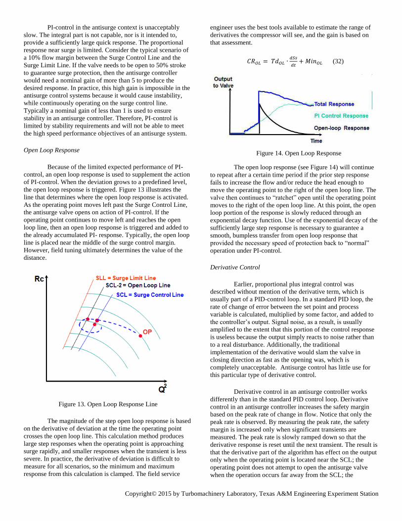
Open Loop Response

Because of the limited expected performance of PI-

control, an open loop response is used to supplement the action

of PI-control. When the deviation grows to a predefined level,

the open loop response is triggered. Figure 13 illustrates the

line that determines where the open loop response is activated.

As the operating point moves left past the Surge Control Line,

the antisurge valve opens on action of PI-control. If the

operating point continues to move left and reaches the open

loop line, then an open loop response is triggered and added to

the already accumulated PI- response. Typically, the open loop

line is placed near the middle of the surge control margin.

However, field tuning ultimately determines the value of the

distance.

Figure 13. Open Loop Response Line

The magnitude of the step open loop response is based

on the derivative of deviation at the time the operating point

crosses the open loop line. This calculation method produces

large step responses when the operating point is approaching

surge rapidly, and smaller responses when the transient is less

severe. In practice, the derivative of deviation is difficult to

measure for all scenarios, so the minimum and maximum

response from this calculation is clamped. The field service

engineer uses the best tools available to estimate the range of

derivatives the compressor will see, and the gain is based on

that assessment.

𝐶𝑅𝑂𝐿 = 𝑇𝑑𝑂𝐿 ∙𝑑𝑆𝑠

𝑑𝑡+ 𝑀𝑖𝑛𝑂𝐿 (32)

Figure 14. Open Loop Response

The open loop response (see Figure 14) will continue

to repeat after a certain time period if the prior step response

fails to increase the flow and/or reduce the head enough to

move the operating point to the right of the open loop line. The

valve then continues to “ratchet” open until the operating point

moves to the right of the open loop line. At this point, the open

loop portion of the response is slowly reduced through an

exponential decay function. Use of the exponential decay of the

sufficiently large step response is necessary to guarantee a

smooth, bumpless transfer from open loop response that

provided the necessary speed of protection back to “normal”

operation under PI-control.

Derivative Control

Earlier, proportional plus integral control was

described without mention of the derivative term, which is

usually part of a PID-control loop. In a standard PID loop, the

rate of change of error between the set point and process

variable is calculated, multiplied by some factor, and added to

the controller’s output. Signal noise, as a result, is usually

amplified to the extent that this portion of the control response

is useless because the output simply reacts to noise rather than

to a real disturbance. Additionally, the traditional

implementation of the derivative would slam the valve in

closing direction as fast as the opening was, which is

completely unacceptable. Antisurge control has little use for

this particular type of derivative control.

Derivative control in an antisurge controller works

differently than in the standard PID control loop. Derivative

control in an antisurge controller increases the safety margin

based on the peak rate of change in flow. Notice that only the

peak rate is observed. By measuring the peak rate, the safety

margin is increased only when significant transients are

measured. The peak rate is slowly ramped down so that the

derivative response is reset until the next transient. The result is

that the derivative part of the algorithm has effect on the output

only when the operating point is located near the SCL; the

operating point does not attempt to open the antisurge valve

when the operation occurs far away from the SCL; the


antisurge valve opens earlier when transients are high in

vicinity of the SCL, and stays closed longer when transients are

no longer present.

Another benefit of this type of derivative control is

that less flow margin is needed between the surge line and the

control line. In other words, if flows and pressures are

reasonably steady then a properly tuned PI- control is adequate

to be used alone. As disturbances increase, derivative control

shifts the control line to the right. Therefore, PI-control has

more room to overshoot when transients exist, and the

compressor has more turndown when the system states remain

relatively unchanged.

Surge Detection

Surge detection algorithms are used to alarm operators and to

possibly shut down a compressor when all other methods of

surge prevention have failed. A compressor’s surge limit line

will, over time, shift because of slowly deteriorating

performance. As the surge line changes, the controller will have

less time to react because the distance between actual surge and

the controller’s surge control line will decrease. If the

compressor surges as a result of its shifted SLL, then the

antisurge controller clearly needs to adapt its configuration by

increasing the safety margin. This adaptive action prevents

further surging by causing the antisurge controller to open the

recycle valve at a higher flow rate.

Figure 15 Surge Detection

Because of its use as an independent layer of defense,

surge detection must use something other than the surge limit

line as a measure. Various ideas related to vibration and special

instrumentation have been proposed as new, additional methods

for surge detection, some of which show great potential.

However, the current “accepted practice” methods used for

surge detection are:

1. Rapid change in flow (See Figure 15)

2. Rapid change in pressure (See Figure 15)

3. Rapid increase in temperature

4. Rapid change in driver power

5. Combinations of items 1-4

There are significant differences between surge

detection and antisurge control that should be noted. Antisurge

control serves the purpose of preventing a compressor from

surging. Surge detection has the purpose of identifying that

surge has occurred or that a compressor is operating at the onset

of surge. Surge detection methods are used in an antisurge

algorithm to enhance and adapt the distance from surge line

calculation. A separate surge detector is used as an independent

protection layer.

Separate Surge Detection as part of the expected 5th

edition of

API 670 Standard

The topic of Surge Detection that makes up the

adaptive feature of the antisurge control algorithm, as discussed

in preceding paragraphs, overlaps with the expected changes in

API 670, 5th edition Machinery Protection Systems.

The 5th edition is expected to have major additions as

it relates to surge detection. The standard is in the process of

approval, but one expected change is that independent surge

detection for axial compressors will be a requirement going

forward. Centrifugal compressors (both inline and integrally

geared) will also be considered as candidates for independent

surge detection if it’s specified or, if the consequence of surge

related damage is unacceptable as defined by the end user or

OEM. In any application for which the consequence of surge

related damage is unacceptable, such as machines with high

pressure ratios or power densities, an independent surge

detection system may be justified. Compressors with multiple

process stages may need surge detection on each stage.

Similarly to an independent overspeed trip device that

is currently required by API 670, independent surge detection

may become a requirement as well. The independent surge

detection is being considered in addition to the expectation of

having antisurge control system used for protection of axial or

centrifugal turbomachinery.

Due to instrumentation malfunctions in transmitters or

control valves, compressor fouling, or failure of the antisurge

control system a compressor may encounter multiple surge

events. If the antisurge control system is unable to prevent

surging, then a surge detection system should be used to

independently detect surge cycling and take action to avoid

severe compressor damage. These surge detectors should use


independent transmitters and independent hardware platforms

to avoid common mode failures. If the antisurge control system

incorporates redundant transmitters and redundant control

elements, it may be allowable for the surge detection function

to be included in the antisurge control system.

Dedicated antisurge control is viewed as the first line

of defense to prevent surge events and is not addressed directly

by API 670. It’s only after the primary antisurge protection is

not effective that independent surge detection is expected to

protect compressor from the surge related damage. If an anti-

surge control system is properly designed and maintained,

machinery damage due to surge events is typically avoided.

The standard allows for multiple surge detection

methods, similar to the ones listed above, and the surge

detection system can incorporate more than one method.

The surge detection system should incorporate a surge

counter that increments for each surge cycle. If more than one

detection method is used, the surge detection system can only

be allowed to identify one surge count per surge event.

The surge detection system would have two outputs,

one for surge alarm and one for excessive surge. The surge

alarm will be activated when a surge event is detected. The

excessive surge output will be activated when a specified

consecutive number of surge cycles are recorded within a

specified time frame. The excessive surge output would be tied

directly to the ESD system to trip the compressor or antisurge

valve.

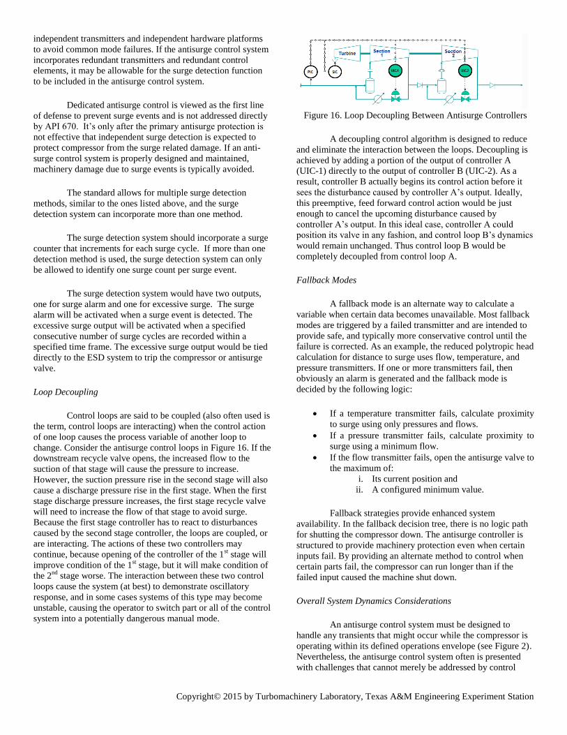
Loop Decoupling

Control loops are said to be coupled (also often used is

the term, control loops are interacting) when the control action

of one loop causes the process variable of another loop to

change. Consider the antisurge control loops in Figure 16. If the

downstream recycle valve opens, the increased flow to the

suction of that stage will cause the pressure to increase.

However, the suction pressure rise in the second stage will also

cause a discharge pressure rise in the first stage. When the first

stage discharge pressure increases, the first stage recycle valve

will need to increase the flow of that stage to avoid surge.

Because the first stage controller has to react to disturbances

caused by the second stage controller, the loops are coupled, or

are interacting. The actions of these two controllers may

continue, because opening of the controller of the 1st stage will

improve condition of the 1st stage, but it will make condition of

the 2nd

stage worse. The interaction between these two control

loops cause the system (at best) to demonstrate oscillatory

response, and in some cases systems of this type may become

unstable, causing the operator to switch part or all of the control

system into a potentially dangerous manual mode.

Figure 16. Loop Decoupling Between Antisurge Controllers

A decoupling control algorithm is designed to reduce

and eliminate the interaction between the loops. Decoupling is

achieved by adding a portion of the output of controller A

(UIC-1) directly to the output of controller B (UIC-2). As a

result, controller B actually begins its control action before it

sees the disturbance caused by controller A’s output. Ideally,

this preemptive, feed forward control action would be just

enough to cancel the upcoming disturbance caused by

controller A’s output. In this ideal case, controller A could

position its valve in any fashion, and control loop B’s dynamics

would remain unchanged. Thus control loop B would be

completely decoupled from control loop A.

Fallback Modes

A fallback mode is an alternate way to calculate a

variable when certain data becomes unavailable. Most fallback

modes are triggered by a failed transmitter and are intended to

provide safe, and typically more conservative control until the

failure is corrected. As an example, the reduced polytropic head

calculation for distance to surge uses flow, temperature, and

pressure transmitters. If one or more transmitters fail, then

obviously an alarm is generated and the fallback mode is

decided by the following logic:

If a temperature transmitter fails, calculate proximity

to surge using only pressures and flows.

If a pressure transmitter fails, calculate proximity to

surge using a minimum flow.

If the flow transmitter fails, open the antisurge valve to

the maximum of:

i. Its current position and

ii. A configured minimum value.

Fallback strategies provide enhanced system

availability. In the fallback decision tree, there is no logic path

for shutting the compressor down. The antisurge controller is

structured to provide machinery protection even when certain

inputs fail. By providing an alternate method to control when

certain parts fail, the compressor can run longer than if the

failed input caused the machine shut down.

Overall System Dynamics Considerations

An antisurge control system must be designed to

handle any transients that might occur while the compressor is

operating within its defined operations envelope (see Figure 2).

Nevertheless, the antisurge control system often is presented

with challenges that cannot merely be addressed by control


algorithms alone. Operation during fast transients, such as ESD,

might require additional equipment (e.g. valves, piping, and

transmitters) to avoid surge. For example consider a system

where the recycle piping is, by layout necessity, comparably

long. In this case, the antisurge system alone will not have the

capability to prevent surge during harsh ESD transients because

the system dynamics of lengthy pipe runs are too slow to be

compensated for by the electronics themselves. In this case a

shorter (often termed “hot-bypass”) recycle pipe run might

need to be installed along with the necessary valves and

instrumentation which is used for the sole purpose of

preventing surge during these harsh transient scenarios. This

additional hot-bypass system needs to be carefully integrated so

its control action will not conflict with the main antisurge

control system. As a general requirement, the antisurge control

system must be able to accept signals from the ESD and other

safety oriented systems protecting the compressor in order to

synchronize its actions with these protective systems.

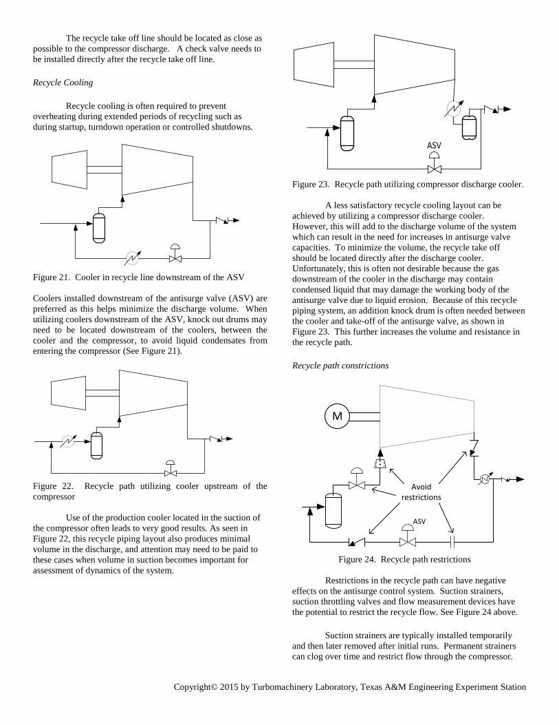
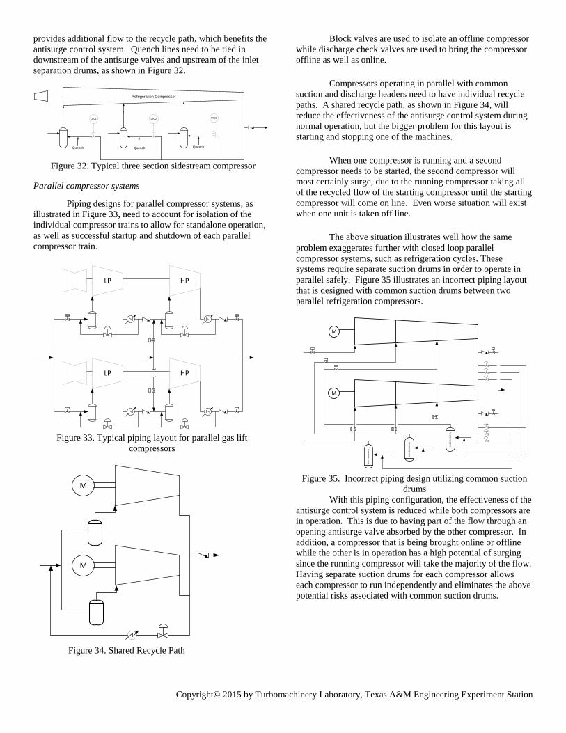
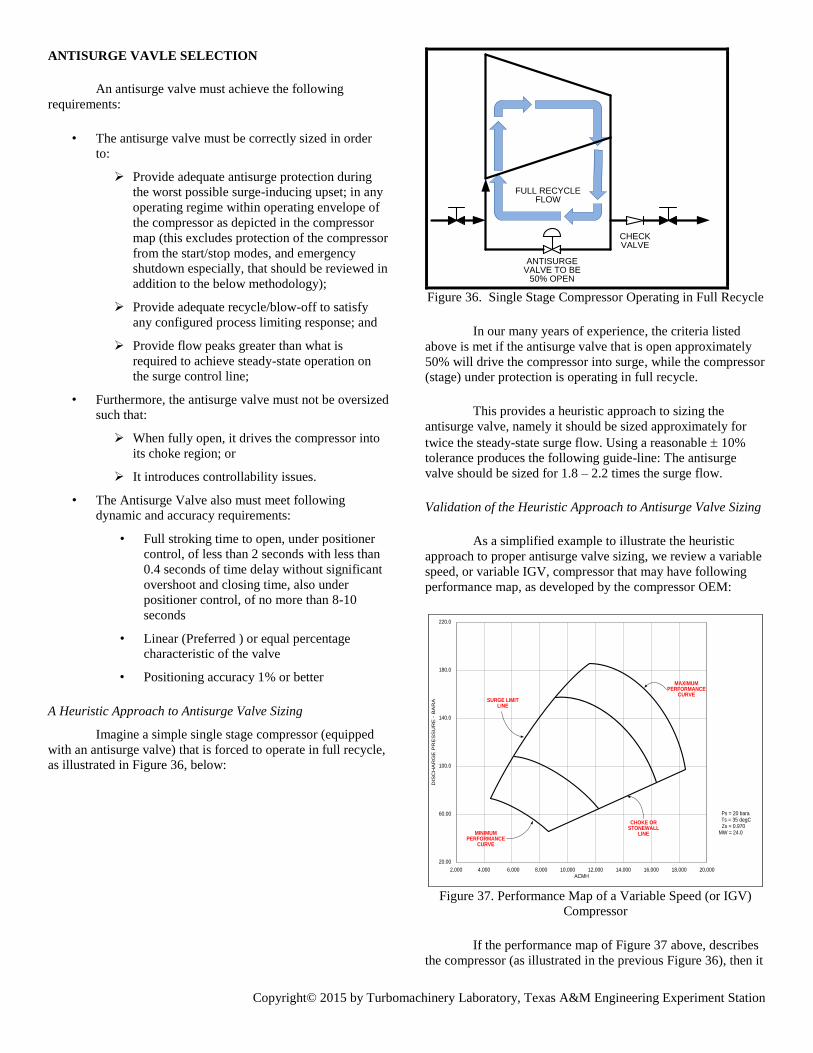
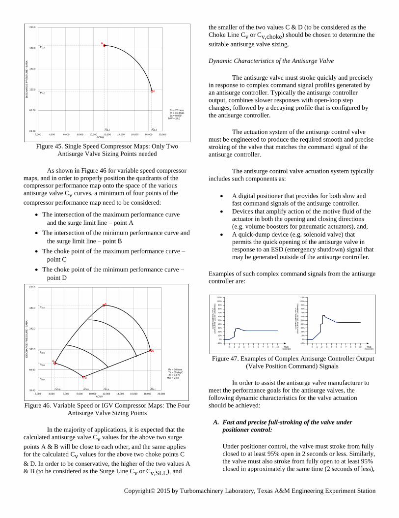
COMBINED ANTISURGE AND PERFORMANCE

CONTROL

The throughput control method has a significant

impact on the antisurge control system. Consider a few

examples: if inlet guide vanes are used, then the antisurge

control system should have inputs and specific

characterizations for the guide vane position; if turbine speed is

controlled, then the antisurge control needs to be integrated to

avoid control loop interactions. In every case, the antisurge and

throughput control are interrelated because they both influence

the same process variables and the same position of the

operating point in the compressor map.

The selection of the compressor drive primarily

depends on size (i.e. power) requirements and available sources

of energy. The throughput control method is usually

predetermined by the drive type. For instance, steam turbines

are often used at refineries and petrochemical plants because

the processes used often produce excess heat that is further

used to produce drive steam as well. In these cases, turbine

speed often becomes the de facto method of throughput control

because the speed can easily be governed with steam flow.

Compressor Throughput Control Methods

A constant speed electric motor driven compressor,

controlled by a suction throttle valve, provides a simple

solution. The startup controls are relatively straightforward and

there is no warm-up sequence, as might be needed in a steam

turbine. No over speed protection is needed. However, the cost

of electricity can be relatively high and throttling inherently

wastes energy. Therefore, constant speed electric motor driven

compressors with throttling used for control are not necessarily

the most energy efficient, but are simple to start and operate.

A constant speed electric motor driven compressor,

controlled by a discharge throttle valve, has similar

characteristics to that of a suction throttle. Both are relatively

easy to operate and maintain. However, for an equivalent

reduction in throughput, suction throttling uses less power

because the inlet gas density is reduced. Additionally, discharge

throttling has substantially stronger negative effect on the

antisurge control then the suction throttling. Therefore suction

throttling is recommended over discharge throttling as a

compressor throughput control method.

Constant speed compressors controlled by inlet guide

vanes are more complicated than suction throttle machines, but

are also more efficient. Inlet guide vanes effectively change the

compressor performance characteristics at each vane angle.

Therefore as the guide vanes open, not only does the flow

increase but the performance curve steepness and surge flow

changes as well (see Compressor with Inlet Guide Vanes on

page 8).

Applications using turbine driven compressors are

usually more efficient than throttled compressors because of the

losses associated with throttling. The machine speed is varied

until the flow requirement at a given pressure ratio is met.

However, turbines (gas or steam) require complicated start-up

and warm-up sequences. Over speed protection controls are

also required on turbines.

Variable frequency drives (VFD) provide an efficient

means for starting and controlling the speed of an electric

motor. As technology improves, such drives have gained in

popularity. Grounding and harmonic vibrations are some of the

main issues associated with VFD’s.

Electric motors can also vary the drive speed through a

fluid coupling. Guide vanes are used in the fluid coupling to

control the amount of transmitted torque. By varying the torque

to the compressor shaft, speed can be controlled. Closed loop

speed control greatly improves the response time and accuracy

of this throughput method. Absence of speed control leads to

the compressor operating at fluctuating speeds as the load

changes, and thus results in poorer quality of throughput

control and possibly a negative impact on the capability of the

antisurge control to protect the compressor. Drawbacks of this

approach are loss of efficiency and increased machine

complexity.

Loop Decoupling

As mentioned previously, loop decoupling is an

important part of an integrated control system. The previous

discussion was on the benefits of loop decoupling between

antisurge peers, and here the benefits of decoupling between

the performance controller and antisurge controller is

investigated. Loop decoupling between a performance

controller and antisurge controller is important because the

antisurge controller is essential to control flow in proximity to

the surge limit line in the compressor map. At the surge control

line, which is located in vicinity of the surge limit line, very

small changes in pressure may cause large changes in flow.

This increases the effect the antisurge controller (UIC), through

operation of the recycle valve, will have on the parameter - like

pressure, or flow that is being controlled by the performance

controller (PIC) in controller interactions (see Figure 16).


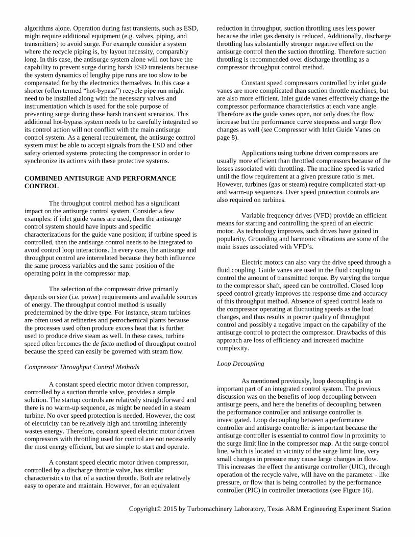
Figure 17. Loop Decoupling Between Antisurge and

Performance Controllers

The first example of loop decoupling is between a

throttle valve and the antisurge valve. In many cases, piping

designs have the suction throttle inside the antisurge loop as

shown in Figure 17. As the antisurge valve opens, pressure

builds in the suction drum. As the suction drum pressure builds,

the performance controller opens the inlet throttle valve to

maintain the pressure. When the performance controller opens

its valve, more flow is introduced into the loop. The antisurge

controller then closes the recycle valve to compensate for this

extra flow and the cycle repeats. The described interaction

negatively affects the quality of control of the process variable,

pressure in this example, making the system behavior more

oscillatory, and potentially unstable. This negative interaction

also affects the antisurge control by allowing wider excursions

of the operating point towards the surge limit line.

A solution to this problem is to feed forward the

antisurge control output to the performance controller. This

feed forward control action eliminates controller oscillations

caused by all of the piping and drum volumes between the

antisurge valve and the suction throttle valve. Consider the

previous example with loop decoupling implemented. As the

antisurge valve opens, the performance control receives a feed

forward command to open its valve as well. The additional gas

flowing into the suction drum due to the increase in the recycle

valve opening is immediately offset by the increase of the

outflow from the suction drum by an increase in the opening of

the inlet throttle control valve. Because the suction drum

pressure remains constant, the performance controller does not

need to act on an additional error through its PID-algorithm. As

a result of decoupling, the antisurge controller (UIC) is free to

maintain position of the operating point relative to the surge

limit line without disturbing the controlled variable of the

performance controller (PIC).

It is worth mentioning that for the common piping

arrangement used in the prior example, the suction throttle

valve should have a mechanical minimum stop. The reason for

this stop is to ensure operability of the antisurge control system

during periods of low load. Typically this stop is initially

implemented at a 15% valve opening, although the final value

is determined at commissioning.

The next example is the interaction observed on a

variable speed machine and the antisurge loop. Figure

18Error! Reference source not found. illustrates a control

interaction scenario where the compression train flow is

reduced to the point where the antisurge valve must open.

Starting at point A, the flow reduction causes discharge

pressure (Pd) to increase. To maintain the controller set point,

the machine speed must decrease. When the speed decreases to

point B, the recycle valve must open to maintain position of the

operating point on the surge control line. At this point, the

speed control loop and antisurge control loop have conflicting

goals: one controller acts to decrease the machine flow while

the other acts to increase it. The overshoot illustrated in Figure

18 can be greatly reduced through loop decoupling. At point B,

a portion of the antisurge output is added to the control

response of the speed controller to help offset the conflicting

control actions. The overall result is the operating point moving

from point B to point C without overshooting the set point

while maintaining a further distance from the Surge Limit Line.

Figure 18. Control Loop Interactions with a Speed Controller

Parallel Train Operation

Often, multiple compressors will work in parallel to

meet the design requirements of a particular installation site.

For instance, LNG plants might use three propane refrigeration

compressors in parallel rather than one large machine. The

machines can be sized so that the plant can operate with two

out of three machines running while one machine is being

serviced. Additionally, if the plant load is greatly reduced,

machines can be taken off line. Using multiple machines

greatly increases the flow range that can be handled by a

particular installation. However, controlling parallel

compressors to efficiently and effectively meet the process

goals can be a challenging task.

The first objective of parallel operation is control of

the main process variable. This main process variable is usually

suction header pressure, discharge header pressure, or

compressor mass flow. The problem with multiple compressors

trying to control, say, suction header pressure is that there are


too many degrees of freedom. For example, suction pressure

header could possibly be maintained with one train fully loaded

while the other train is in full recycle. The same suction header

pressure could also be maintained by both machines operating

at part load. If each train uses an independent controller to

maintain a common suction header pressure, the two controllers

will constantly oscillate back and forth.

Load Sharing Controller


Master

Load Sharing response

Load Sharing response

Figure 19. Load Sharing response

To maintain the main process variable, a single master

controller needs to manage the main control variable. By using

a single controller, the degrees of freedom are reduced to one:

one control output is governed by a single input. If the master

controller needs lower suction header pressure, it commands

both load sharing controllers to increase its output by an equal

amount. This control architecture guarantees that both

compressor trains are intended to move in the same direction to

meet the main process goal. Figure 19 shows a block diagram

of the Load Sharing response.

The parallel control strategy thus far hasn’t solved the

problem of balancing the trains. Since no two compressors are

exactly alike, the control system must take into account that

each compressor will handle flow differently. The point/flow at

which a compressor surges is one of the best indications for the

machine’s ability to handle flow. If one compressor is on the

verge of surging while its peer has twice the surge flow, then

clearly the best solution is to take flow from the latter and send

it to the former. Eventually, the optimal point would be reached

when each machine is as far away from surge as possible, and

both are located at the same distance from their surge line.

Therefore equalizing the relative distance from surge, or

deviation, is the best means for distributing flow amongst

parallel compressors. This strategy guarantees minimum overall

recycle of the group of compressors, thus providing for the

most efficient operation. This same strategy also guarantees

the most effective antisurge control, because in the case of a

disturbance, all compressors in the parallel system begin to

open their recycle valves at the same time - without leaving one

of the compressors behind, thus endangering it.

In order to balance the trains based on Deviation from

SCL, the antisurge controllers are included into the control

strategy. On each train, all stages of the train report their

distance from surge to the local performance controller. This

local performance (Load Sharing) controller then applies some

logic (usually the minimum of the reported distances) and

reports the result to the master controller. The Master controller

then uses the average of the reported deviations as a set point

command to each load sharing controller. Figure 20 illustrates

the load balancing control strategy.


SP = Avg. DeviationPV = Min. Deviation

Master

Average Deviation

Average Deviation

Antisurge Controller




Deviation

Deviation

Minimum Deviation


SP = Avg. DeviationPV = Min. Deviation

Minimum Deviation

Deviation

Deviation

Load Sharingresponse

Load Sharingresponse

Figure 20. Parallel Load Sharing and Load Balancing

In practice, the single master controller sends two

signals to each of the associated train controllers. The first

signal is a direct command to increase or decrease the

controller output depending on the needs of the main process

variable control. The second signal is a set point that is the

average distance of all compressors from surge. The overall

output from the load sharing controller is then the sum of its

own PI-control loop used to balance the deviation, and the load

sharing response from the master controller used to maintain

the primary process variable.

PIPING DESIGN CONSIDERATIONS

Piping system around the compressor must be

designed to minimize the volume in the compressor discharge,

between the compressor discharge flange, the inlet of the

antisurge valve and the non-return (check) valve as much as

possible. Large gas volumes act as energy storage, slowing

recycle response times and increasing danger to the compressor

during execution of protection cycle. Additionally, it is useful

to note that the degree of damage to the compressor in an

undesired case of compressor surge depends on the volume of

gas in the compressor discharge The relationship is pretty

straightforward, the higher the volume, the longer it will take to

pass back through the compressor, and consequently, the higher

the damage to the compressor internals.


The recycle take off line should be located as close as

possible to the compressor discharge. A check valve needs to

be installed directly after the recycle take off line.

Recycle Cooling

Recycle cooling is often required to prevent

overheating during extended periods of recycling such as

during startup, turndown operation or controlled shutdowns.

Figure 21. Cooler in recycle line downstream of the ASV

Coolers installed downstream of the antisurge valve (ASV) are

preferred as this helps minimize the discharge volume. When

utilizing coolers downstream of the ASV, knock out drums may

need to be located downstream of the coolers, between the

cooler and the compressor, to avoid liquid condensates from

entering the compressor (See Figure 21).

Figure 22. Recycle path utilizing cooler upstream of the

compressor

Use of the production cooler located in the suction of

the compressor often leads to very good results. As seen in

Figure 22, this recycle piping layout also produces minimal

volume in the discharge, and attention may need to be paid to

these cases when volume in suction becomes important for

assessment of dynamics of the system.

ASV

Figure 23. Recycle path utilizing compressor discharge cooler.

A less satisfactory recycle cooling layout can be

achieved by utilizing a compressor discharge cooler.

However, this will add to the discharge volume of the system

which can result in the need for increases in antisurge valve

capacities. To minimize the volume, the recycle take off

should be located directly after the discharge cooler.

Unfortunately, this is often not desirable because the gas

downstream of the cooler in the discharge may contain

condensed liquid that may damage the working body of the

antisurge valve due to liquid erosion. Because of this recycle

piping system, an addition knock drum is often needed between

the cooler and take-off of the antisurge valve, as shown in

Figure 23. This further increases the volume and resistance in

the recycle path.

Recycle path constrictions

ASV

Avoid restrictions

M

Figure 24. Recycle path restrictions

Restrictions in the recycle path can have negative

effects on the antisurge control system. Suction strainers,

suction throttling valves and flow measurement devices have

the potential to restrict the recycle flow. See Figure 24 above.

Suction strainers are typically installed temporarily

and then later removed after initial runs. Permanent strainers

can clog over time and restrict flow through the compressor.


Permanent strainers, as well as temporary strainers, require

additional instrumentation to measure the pressure drop across

the strainer in order to determine if the strainer is becoming

clogged.

Suction throttle valves should be installed upstream of

the recycle path intake. Throttling downstream of the recycle

path in take may be necessary, for example, to prevent high

motor current during the startup of the compressor, a minimum

mechanical stop should be incorporated on the valve to ensure

that there will always be the necessary recycle flow to the

compressor in case of valve failure or accidental closure.

Flow measurement devices are sometimes installed in

the recycle line to measure the amount of recycle flow. Flow

measurement devices with high permanent pressure loss should

be avoided. An alternative method of measuring recycle flow

is to install the flow measuring device downstream of the

recycle line take off and subtract this flow from the compressor

throughput flow measured by the antisurge control system.

Some compressor manufacturers may require a check

valve to be installed directly after the compressor’s discharge

flange to prevent reverse flow through the compressor. In these

cases, a non-slam type check valve should be used. Check

valves located in the recycle line should be avoided as there is

the possibility of the check valve becoming stuck closed and

preventing recycle flow.

Multi-case compressors

Multi-case compressors as shown in Figure 25 are

among the most complex compressors in use. The equivalent of

two or more machines driven by a common driver, they can

produce large compression ratios and are used extensively in

wet-gas, gas gathering, and other applications. Although the

below discussion focuses on two stage compressors, three, four,

and more stage multi-case compressors are commonly used

throughout the industry as well. These compressors can have

complicated piping designs depending on the process

requirements.

Low Pressure Case High Pressure Case

Figure 25. Typical two stage multi-case compressor

Even though all rotors are driven by the same driver,

each stage has its own unique set of operating variables and

disturbances to contend with. Efficiency, inlet and outlet

temperatures, and pressures, gas composition, specific heat

ratio, and compressibility all figure into the problem, yet vary

from stage to stage. Each stage can surge independently of the

others and must be protected as if it were a separate machine.

For the fastest response, each compressor section should have

its own recycle line with a cooler and be controlled by an

individual antisurge control loop reflecting properties of this

compression stage, as shown in Figure 26. As discussed above,

existing process coolers can be used as well.


Figure 26. Two stage compressor with individual recycle

paths

Examples of Compromised Piping Designs

Figure 27 illustrates a two-case machine in which both

recycle lines are cooled by the same heat exchanger. Although

this reduces capital and installation expenses, the large common

cooler required by such an arrangement tends to bring

additional, sometimes unacceptably high, dynamic instability

between the two antisurge control loops.


Figure 27. Recycle cooling using common inter-stage cooler

For example, when the antisurge valve for the high-

pressure case opens, flow through the high-pressure case

increases almost immediately. This loop’s time constant is

small because the volume between its antisurge valve and

discharge is small. Because of the large inter-stage cooler there

is a large volume in the low-pressure case’s recycle line which

may be further worsened by additional volume due to the

potential need of a discharge knock out drum. The time

constant of this section’s antisurge control loop is much larger

because of the inertial mass of the extra gas. This can lead to

adverse control interaction.

Suppose the high-pressure case is moving towards its

surge limit and starts to recycle to avoid surge. The discharge

pressure in the low-pressure case will rise rapidly because the

high-pressure recycle line feeds into the low-pressure case’s

discharge.

As this pressure rises, the first section’s controller

reaches its surge control line and opens its antisurge valve to

lower the pressure. However, low-pressure section discharge

pressure is dominated by high-pressure recycle and continues to


rise. When the low-pressure case starts to recycle, it

immediately diverts flow from the suction of the high-pressure

case. The high-pressure case must then increase its recycle to

make up for the extracted flow, driving discharge pressure at

the low-pressure case even higher. The net effect of low-

pressure section recycle may be to increase in the first few

seconds, rather than decrease the discharge pressure of that

stage, thus possibly resulting in the section failing to avoid

surge.

Adding a cooler to each recycle line is an ideal

solution, but it is not the only solution. The system can be

improved by changing the piping to include the upstream

process cooler and an addition of a check valve between stages,

as shown in Figure 28 below. This approach almost completely

eliminates the problems inherent in the original layout shown in

Figure 27.


Figure 28. Improved piping design

The volumes between each compressor discharge and

antisurge valve are small, so both antisurge controllers can be

tuned aggressively. This keeps recycling to an energy-efficient

minimum. Because the two loops have similar time constants,

controller interactions are less dramatic and decoupling more

effective.

Single overall recycle line across multiple stages

Figure 29 shows a two stage compressor with a single

overall recycle path. Using a single recycle path is sometimes

employed as the main method of avoiding interactions between

individual antisurge control loops, as in Figure 28. This

solution can result in excessive recycle and degrades surge

protection. For example in Figure 29, the single recycle path

may offer adequate protection for the high-pressure case, but it

protects the low pressure case very poorly. The possible large

time delay and lag before the discharge pressure of the low-

pressure case decreases may present challenges when operating

near its surge limit.


Figure 29. Two-stage compressor with one overall recycle path

Process applications that do not require recycling the

gas such as process air compressors use blow off lines to

provide antisurge protection. Process air compressors and air

blowers which can have up to five or six stages can be

effectively controlled utilizing a single blow off line located in

the discharge, as shown in Figure 30. Additional blow off lines

and valves may be required on these machines to accommodate

substantial differences in surge flow on lower pressure stages.

PROCESS AIR COMPRESSOR

Blow Off Valve

Figure 30. Typical Process Air Compressor

Multi-sectional compressors

Multi-sectional compressors with sidestreams, such as

those used in refrigeration processes, differ from multi-case

compressors in that all the compressor section recycle lines

have the take-off from the discharge of the compressor. See

Figure 31 below. This piping arrangement introduces time

delays in the overall response of the system. Reduction in head

across the compressor is less effective as a means of protecting

the compressor from surge. Therefore increasing flow through

each section becomes the primary means for surge prevention.

Refrigeration Compressor

UIC1 UIC2 UIC3

Figure 31. Typical three section sidestream compressor

Although opening the first section’s antisurge valve

will benefit the following stages by increasing throughput,

opening of downstream section’s antisurge valve can have

negative effects on upstream sections. For example, when the

third section antisurge valve opens, the pressure in the second

section discharge increases, as does the resistance. This tends

to drive the second section towards surge. To overcome this

and the lag times associated with longer recycle lines, loop

decoupling, as described earlier, should be established between

the downstream and upstream section antisurge controllers.

For example in Figure 31, antisurge controller UIC1 should

decouple from UIC2 and UIC3, while antisurge controller

UIC2 should decouple from UIC3.

Multi-sectional compressors with sidestreams often

utilize liquid quench to cool the recycle gas. Using liquid

quench to cool the recycle gas, instead of discharge process

coolers, helps reduce the large discharge volumes that are

typically associated with refrigeration cycles. Also, quench


provides additional flow to the recycle path, which benefits the

antisurge control system. Quench lines need to be tied in

downstream of the antisurge valves and upstream of the inlet

separation drums, as shown in Figure 32.

Quench Quench Quench

Refrigeration Compressor

UIC1 UIC2 UIC3

Figure 32. Typical three section sidestream compressor

Parallel compressor systems

Piping designs for parallel compressor systems, as

illustrated in Figure 33, need to account for isolation of the

individual compressor trains to allow for standalone operation,

as well as successful startup and shutdown of each parallel

compressor train.

LP HP

LP HP

Figure 33. Typical piping layout for parallel gas lift

compressors

M

M

Figure 34. Shared Recycle Path

Block valves are used to isolate an offline compressor

while discharge check valves are used to bring the compressor

offline as well as online.

Compressors operating in parallel with common

suction and discharge headers need to have individual recycle

paths. A shared recycle path, as shown in Figure 34, will

reduce the effectiveness of the antisurge control system during

normal operation, but the bigger problem for this layout is

starting and stopping one of the machines.

When one compressor is running and a second

compressor needs to be started, the second compressor will

most certainly surge, due to the running compressor taking all

of the recycled flow of the starting compressor until the starting

compressor will come on line. Even worse situation will exist

when one unit is taken off line.

The above situation illustrates well how the same

problem exaggerates further with closed loop parallel

compressor systems, such as refrigeration cycles. These

systems require separate suction drums in order to operate in

parallel safely. Figure 35 illustrates an incorrect piping layout

that is designed with common suction drums between two

parallel refrigeration compressors.

M

M

SU

CT

ION

DR

UM

SU

CT

ION

DR

UM

SU

CT

ION

DR

UM

Figure 35. Incorrect piping design utilizing common suction

drums

With this piping configuration, the effectiveness of the

antisurge control system is reduced while both compressors are

in operation. This is due to having part of the flow through an

opening antisurge valve absorbed by the other compressor. In

addition, a compressor that is being brought online or offline

while the other is in operation has a high potential of surging

since the running compressor will take the majority of the flow.

Having separate suction drums for each compressor allows

each compressor to run independently and eliminates the above

potential risks associated with common suction drums.


ANTISURGE VAVLE SELECTION

An antisurge valve must achieve the following

requirements:

• The antisurge valve must be correctly sized in order

to:

Provide adequate antisurge protection during

the worst possible surge-inducing upset; in any

operating regime within operating envelope of

the compressor as depicted in the compressor

map (this excludes protection of the compressor

from the start/stop modes, and emergency

shutdown especially, that should be reviewed in

addition to the below methodology);

Provide adequate recycle/blow-off to satisfy

any configured process limiting response; and

Provide flow peaks greater than what is

required to achieve steady-state operation on

the surge control line;

• Furthermore, the antisurge valve must not be oversized

such that:

When fully open, it drives the compressor into

its choke region; or

It introduces controllability issues.

• The Antisurge Valve also must meet following

dynamic and accuracy requirements:

• Full stroking time to open, under positioner

control, of less than 2 seconds with less than

0.4 seconds of time delay without significant

overshoot and closing time, also under

positioner control, of no more than 8-10

seconds

• Linear (Preferred ) or equal percentage

characteristic of the valve

• Positioning accuracy 1% or better

A Heuristic Approach to Antisurge Valve Sizing

Imagine a simple single stage compressor (equipped

with an antisurge valve) that is forced to operate in full recycle,

as illustrated in Figure 36, below:

CHECKVALVE

ANTISURGEVALVE TO BE

50% OPEN

FULL RECYCLE FLOW

Figure 36. Single Stage Compressor Operating in Full Recycle

In our many years of experience, the criteria listed

above is met if the antisurge valve that is open approximately

50% will drive the compressor into surge, while the compressor

(stage) under protection is operating in full recycle.

This provides a heuristic approach to sizing the

antisurge valve, namely it should be sized approximately for

twice the steady-state surge flow. Using a reasonable 10%

tolerance produces the following guide-line: The antisurge

valve should be sized for 1.8 – 2.2 times the surge flow.

Validation of the Heuristic Approach to Antisurge Valve Sizing

As a simplified example to illustrate the heuristic

approach to proper antisurge valve sizing, we review a variable

speed, or variable IGV, compressor that may have following

performance map, as developed by the compressor OEM:

20.00

60.00

100.0

140.0

180.0

220.0

2,000 6,000 10,000 14,0004,000 8,000 12,000 16,000 18,000 20,000

Ps = 20 baraTs = 35 degCZs = 0.970

MW = 24.0

ACMH

DIS

CH

AR

GE

PR

ES

SU

RE

- B

AR

A

CHOKE OR STONEWALL

LINE

SURGE LIMIT LINE

MAXIMUM PERFORMANCE

CURVE

MINIMUM PERFORMANCE

CURVE

Figure 37. Performance Map of a Variable Speed (or IGV)

Compressor

If the performance map of Figure 37 above, describes

the compressor (as illustrated in the previous Figure 36), then it


is possible to “super-impose” lines of antisurge valve capacity,

Cv onto it, yielding the following combined performance map

(Figure 38):

20.00

60.00

100.0

140.0

180.0

220.0

2,000 6,000 10,000 14,0004,000 8,000 12,000 16,000 18,000 20,000


MW = 24.0

ACMH

DIS

CH

AR

GE

PR

ES

SU

RE

- B

AR

A

Cv = 30 Cv = 40 Cv = 50 Cv = 60 Cv = 70 Cv = 80 Cv = 90

Cv = 180 Cv = 190

Cv = 210Cv = 230

SURGE CONTROL LINEAPPROX. 10% OF SURGE FLOW TO THE

RIGHT OF THE SLL

Cv,valve,min =

135

Cv,valve,max =

165

Figure 38. Antisurge Valve Cv curves superimposed onto the

Compressor Performance Map

As seen in Figure 38, an antisurge valve with a Cv value of

approximately 75 would provide the minimum steady-state

antisurge flow to keep the compressor in full recycle. Thus,

according to the “1.8 – 2.2 times the surge flow” guideline, a

valve with a full-stroke Cv value of between 135 and 165

should be used for antisurge duty for this compressor.

With the compressor operating in a full recycle mode, such a

valve, even when fully opened, would not have the capacity to

drive the compressor into its choke region (that would occur for

a Cv > 220).

ISA Valve Sizing Equation

The ISA valve sizing equation (ISA-S75.01-1985) based on

mass flow through the valve is used. This equation is:

MW

1Z

1T

Y1

Pp

F N

W= Cv

8

S

X(33)

Deriving the Mass Flow (WS) through the Antisurge Valve

Applications Where the Antisurge Line Spans A Single

Compressor Section

CHECKVALVE

PS

TS

ZS

MW

kS

WS

CHECKVALVE

PS

TS

ZS

MW

kS WS

RECYCLE VALVE

BLOWOFFVALVE

QS QS

Figure 39. Antisurge Line Spans A Single Compressor Section

Imagine the compressor as operating in full recycle (left pane

of above Figure 39), or full blow-off (right pane of above).

The volumetric flow rate at the Surge Point QSLL

is determined

from the supplied compressor performance curves. The

equivalent mass flow rate (WSLL

) is then calculated and this is

used for antisurge valve sizing purposes.

WSLL

= QSLL

S (34)

where:

S

𝑃𝑆∗𝑀𝑊

𝑍𝑆∗𝑅𝑂∗𝑇𝑆 (35)

Applications with Sidestream Compressors

Sidestream compressors present more challenge to the

previous approach of using the surge flow at the maximum

performance curve, as previously described. This is because

each stage’s performance curve is given for conditions at the

common RATED speed for all the stages. A slightly different,

but fundamentally similar approach is used. The first step, the

same as in the example above is to establish steady-state mass

flow rates for all stages of the compression that are then

increased by using the same heuristic method as above.

1.00

2.00

3.00

4.00

LP STAGE

2,000 6,000 10,0004,000 8,000

PS,LP = 1.20 baraTS,LP = -35 degCZS,LP = 1.000

MWLP = 42.0

SUCTION VOLUMETRIC FLOW - ACMH

DIS

CH

AR

GE

PR

ES

SU

RE

- B

AR

A

RATED OPERATING POINT

QS,LP

100% SPEED

3.00

5.00

7.00

9.00

0 2,0001,000 3,000

PS,MP = 3.00 baraTS,MP = -5 degCZS,MP = 0.980

MWMP = 42.0


100% SPEED

5.00

10.00

15.00

20.00

0 600 1,000400 800

PS,HP = 7.00 baraTS,HP = 10 degCZS,HP = 0.970

MWHP = 42.0


100% SPEED

QS,MP QS,HP

MP STAGELP STAGE HP STAGE

Figure 40. Compressor Maps for a 3-Stage Sidestream

Compressor

As may be seen in Figure 40, a horizontal line is

drawn that passes through each stage’s rated point. Where this

horizontal line intersects with the surge limit line, the suction

volumetric flow (QSLL

) is noted.

Next, it is imagined that the compressor operates in

full recycle, as per the following Figure 41:


CHECKVALVE

LPSTREAM

MPSTREAM

HPSTREAM

WS,V,LP

PS,LP

TS,LP

ZS,LP

MWLP

kS,LP

QS,LP

WSS,MP

QS,MP

WS,LP

PS,MP

TS,MP

ZS,MP

MWMP

kS,MP

WS,MP

WS,V,MP

WSS,HP

WS,V,HP

QS,HP

WS,HP

PS,HP

TS,HP

ZS,HP

MWHP

kS,HP

Figure 41. 3-Stage Sidestream Compressor in Full Recycle

For the LP stage, determining the mass flow for the LP

antisurge valve calculations is straightforward. It will be the

mass flow that corresponds to the LP stage surge Limit Line

volumetric flow, as derived above, and where density S,LP

is

calculated as per equation (35) above:

WSLL,LP

= QSLL,LP

S,LP

(36)

For the MP stage, we first determine the surge limit

line mass flow from the MP stage surge limit line volumetric

flow using density S,MP

, as derived above:

WSLL,MP

= QSLL,MP

S,MP

(37)

In the assumed steady-state full recycle situation, the

MP stage thus requires a steady-state mass flow rate equivalent

to the above-derived WSLL,MP

. But the MP stage is already

receiving a mass flow equivalent to WSLL,LP

, coming from the

LP stage (which may be considered as credit), and so, the MP

antisurge valve needs to supply only an additional steady-state

mass flow amount WV,MP

equal to:

WV,MP

= WSLL,MP

- WSLL,LP

(38)

For the HP stage, a similar approach is adopted: We

first determine the Surge Limit Line mass flow from the HP

stage Surge Limit Line volumetric flow, as derived above:

WSLL,HP

= QSLL,HP

S,HP

(39)

In the assumed steady-state full recycle situation, the

HP stage thus requires a steady-state mass flow rate equivalent

to the above-derived WSLL,HP

. But the HP stage is already

receiving a mass flow equivalent to WSLL,MP

, coming from the

MP stage (which may be considered as credit), and so, the HP

antisurge valve needs to supply only a steady-state mass flow

amount WV,HP

equal to:

WV,HP

= WSLL,HP

- WSLL,MP

(40)

Deriving the Antisurge Valve Inlet Pressure P1 and Outlet

Pressure P2

CHECKVALVE

PRESSURE DROP ACROSS DISCHARGE

PROCESS EQUIPMENT

PRESSURE DROP ACROSS SUCTION

PROCESS EQUIPMENT

P2 P1

DPs

DPd

Ps

Pd

Figure 42. Deriving the Antisurge Valve Inlet (P1) and Outlet

(P2) Pressures

As may be seen from Figure 42 above, the antisurge

valve inlet pressure value P1, for antisurge valve sizing

calculation purposes, should be determined by accounting for

all the pressure losses DPd between the compressor stage

discharge flange and the antisurge valve inlet:

P1 = Pd - DPd (41)

Likewise, the antisurge valve outlet pressure value P2,

for antisurge valve sizing calculation purposes, should be

determined by accounting for all the pressure losses DPS

between the compressor stage inlet flange and the antisurge

valve outlet:

P2 = PS + DPS (42)

Deriving the Antisurge Valve Inlet Temperature T1

In most applications, the antisurge valve is located

downstream of an aftercooler, so that the piping configuration

looks like the following Figure 43:

CHECKVALVE

T1

Td

TAC

Figure 43. Deriving the Antisurge Valve Inlet

Temperature (T1) – Case 1


In this case, the antisurge valve inlet temperature T1

may be assumed as being equal to the aftercooler design outlet

temperature.

T1 = TAC (43)

In some cases, the antisurge valve is located upstream

of any aftercoolers, i.e. the piping configuration looks like the

following Figure 44:

Figure 44. Deriving the Antisurge Valve Inlet

Temperature (T1) – Case 2

In such applications there is usually some method to

cool the recycle flow, such as a recycle cooler (as illustrated in

the left pane of above Figure 44), or a process cooler (as

illustrated in the right pane of above Figure 44).

In cases such as these, for antisurge valve sizing

calculation purposes, the antisurge valve inlet temperature

value T1 may be determined assuming it is equal to the

compressor outlet flange discharge temperature.

T1 = Td (44)

Deriving Gas Compressibility Factor Z1 at the Antisurge Valve

Inlet

While the actual value of the gas compressibility

factor at the antisurge valve inlet will depend on the pressure

and temperature at various points of the supplied compressor

performance maps, we are assuming the value given on the

compressor data sheets at the discharge flange at design

conditions produces the usual acceptably accurate capacity

calculations. Therefore:

Z1 = Zd,design (45)

Alternatively one of available Gas Equations of State

(EOS) can be used to establish a more accurate value of Z1.

Deriving the Gas Expansion Factor (Y) For Antisurge Valve

Calculations

According the ISA, the following equation produces

the value of the gas expansion factor (Y) at the antisurge valve

inlet:

𝑌 = 1 −𝑋

3∗𝐹𝑘∗𝑋𝑇 (46)

The value of Y is limited at the upper end to 1.0000 and at the

lower end to 0.6667.

Also note that If X > (FK XT), then (FK XT) should be used in

place of X in the equations for Y and CV.

Deriving the Piping Geometry Factor (Fp) For Antisurge Valve

Calculations

According the ISA, the piping geometry factor Fp is calculated

as:

Fp =

2

1

2

21

d

v,vC

890

K1

(47)

Where:

K = K1 + K2 + KB1 - KB2 (48)

K1 =

2

21D

21

d15.0

(49)

K2 =

2

22D

22

d10.1

(50)

KB1 = 4

1D

1d1

(51)

KB2 = 4

2D

2d1

(52)

Where:

K is a factor that accounts for the effective

velocity head coefficients of the fittings attached

to but not including the valve

Antisurge Valve Sizing and Compressor Choke

For single speed compressor maps, only the two end

points of the compressor curve need to be considered: the surge

point (A) and the choke point (C), as shown in Figure 45.


20.00

60.00

100.0

140.0

180.0

220.0

2,000 6,000 10,000 14,0004,000 8,000 12,000 16,000 18,000 20,000


MW = 24.0

ACMH

DIS

CH

AR

GE

PR

ES

SU

RE

- B

AR

A

A

C

QS,A QS,C

PD,A

PD,C

Figure 45. Single Speed Compressor Maps: Only Two

Antisurge Valve Sizing Points needed

As shown in Figure 46 for variable speed compressor

maps, and in order to properly position the quadrants of the

compressor performance map onto the space of the various

antisurge valve Cv curves, a minimum of four points of the

compressor performance map need to be considered:

The intersection of the maximum performance curve

and the surge limit line – point A

The intersection of the minimum performance curve and

the surge limit line – point B

The choke point of the maximum performance curve –

point C

The choke point of the minimum performance curve –

point D

20.00

60.00

100.0

140.0

180.0

220.0

2,000 6,000 10,000 14,0004,000 8,000 12,000 16,000 18,000 20,000


MW = 24.0

ACMH

DIS

CH

AR

GE

PR

ES

SU

RE

- B

AR

A

A

B

C

D

QS,B QS,D QS,A QS,C

PD,A

PD,C

PD,B

PD,D

Figure 46. Variable Speed or IGV Compressor Maps: The Four

Antisurge Valve Sizing Points

In the majority of applications, it is expected that the

calculated antisurge valve Cv values for the above two surge

points A & B will be close to each other, and the same applies

for the calculated Cv values for the above two choke points C

& D. In order to be conservative, the higher of the two values A

& B (to be considered as the Surge Line Cv or Cv,SLL), and

the smaller of the two values C & D (to be considered as the

Choke Line Cv or Cv,choke) should be chosen to determine the

suitable antisurge valve sizing.

Dynamic Characteristics of the Antisurge Valve

The antisurge valve must stroke quickly and precisely

in response to complex command signal profiles generated by

an antisurge controller. Typically the antisurge controller

output, combines slower responses with open-loop step

changes, followed by a decaying profile that is configured by

the antisurge controller.

The actuation system of the antisurge control valve

must be engineered to produce the required smooth and precise

stroking of the valve that matches the command signal of the

antisurge controller.

The antisurge control valve actuation system typically

includes such components as:

A digital positioner that provides for both slow and

fast command signals of the antisurge controller.

Devices that amplify action of the motive fluid of the

actuator in both the opening and closing directions

(e.g. volume boosters for pneumatic actuators), and,

A quick-dump device (e.g. solenoid valve) that

permits the quick opening of the antisurge valve in

response to an ESD (emergency shutdown) signal that

may be generated outside of the antisurge controller.

Examples of such complex command signals from the antisurge

controller are:

-10%

0%

10%

20%

30%

40%

50%

60%

70%

80%

90%

100%

110%

0 1 2 3 4 5 6 7 8 9 10 TIME(Seconds)

CO

NT

RO

LL

ER

OU

TP

UT

(AN

TIS

UR

GE

VA

LV

E C

OM

MA

ND

)

-10%

0%

10%

20%

30%

40%

50%

60%

70%

80%

90%

100%

110%

0 1 2 3 4 5 6 7 8 9 10 TIME(Seconds)

CO

NT

RO

LL

ER

OU

TP

UT

(AN

TIS

UR

GE

VA

LV

E C

OM

MA

ND

)

Figure 47. Examples of Complex Antisurge Controller Output

(Valve Position Command) Signals

In order to assist the antisurge valve manufacturer to

meet the performance goals for the antisurge valves, the

following dynamic characteristics for the valve actuation

should be achieved:

A. Fast and precise full-stroking of the valve under

positioner control:

Under positioner control, the valve must stroke from fully

closed to at least 95% open in 2 seconds or less. Similarly,

the valve must also stroke from fully open to at least 95%

closed in approximately the same time (2 seconds of less),


but in a maximum of 8-10 seconds or less. Significantly

different stroking speeds in opposite directions will

present unequal dynamic gains in the final control element

that could compromise antisurge controller tuning.

-10%

0%

10%

20%

30%

40%

50%

60%

70%

80%

90%

100%

110%

0 1 2 3 4 0 1 2 3 4 TIME(Seconds)

CO

NT

RO

LL

ER

OU

TP

UT

(AN

TIS

UR

GE

VA

LV

E C

OM

MA

ND

)

CUSHIONED LAST 5% OF FULL OPENING OR

CLOSING

BETWEEN 1 TO 2 SECONDS TO TRAVEL

95% OF FULL STROKE IN THE OPENING DIRECTION

NO MORE THAN 0.3 SECONDS DELAY

NO MORE THAN 0.3 SECONDS DELAY

ACTUAL VALVE STROKE

4 SECONDS TO TRAVEL 95% OF FULL STROKE IN

THE CLOSING DIRECTION

Figure 48. Full-Stroke Speed of The Antisurge Valve Under

Positioner Control

To be noted, the above difference in opening and closing

times is not specified for the purposes of the antisurge

control, but should be allowed to enable valve OEM to

deliver the specified valve quality The antisurge controller

must allow for the slow closing of the antisurge valve

following an open-loop step opening of the valve, but it is

recommended that this be achieved electronically within

the controller by means of dedicated algorithms that set

the controller output signal value (controlled decay),

rather than different stroking speeds (depending on the

direction of travel) within the antisurge valve actuation

system.

When the antisurge controller commands the valve to

fully open or close, the valve actuation system must

exhibit no more than a 0.4 second delay time.

Finally, it is recommended that a “cushioning” feature be

implemented in the actuation system (typically in the last

5% of full-stroke) to prevent the actuator from

“slamming” against the mechanical stops at the end of

stroke, which could potentially damage the actuator or the

valve.

B. No significant hysteresis or overshoot of the valve for

partial stroking under positioner control:

The valve must partially stroke for fast or slow command

signals from the antisurge controller without significant

overshoot in either direction, and with a minimum of

hysteresis when the command signal changes direction.

Since the antisurge controller may send the antisurge

valve a command to step open and then resume

modulating control action, it is desirable to have the valve

actuation system achieve the step change (in the opening

direction) with as little instability as possible. Some

“overshoot” (antisurge valve actuation system initially

opens the valve more than the target position then settles

to the target position) may be acceptable, continuous

oscillatory behavior in valve actuation that may cause an

overshoot in close direction is not acceptable.

In general, it is recommended that one-sided “overshoot”

(i.e. in the opening direction only) should not exceed 10-

15% of the step change in the controller output.

It is recommended to subject the antisurge valve with its

actuation system to a controlled performance test at an

internal valve static pressure and flowing conditions

approximating actual process conditions to record the

overshoot for step changes of 10%, 20% and 50%, as

shown in Figure 49.

-10%

0%

10%

20%

30%

40%

50%

60%

70%

80%

90%

100%

110%

0 1 2 3 4 0 1 2 3 4 TIME(Seconds)

CO

NT

RO

LL

ER

OU

TP

UT

(AN

TIS

UR

GE

VA

LV

E C

OM

MA

ND

)

NO SIGNIFICANT OVERSHOOT OR HYSTERESIS IN EITHER DIRECTION FOR VARIOUS STEP CHANGES (E.G. 10%, 20% & 50%)

ACTUAL VALVE

STROKE

Figure 49. Partial-Stroke Testing of The Antisurge Valve

Under Positioner Control

It is also recommended to test the valve by imposing a

continuously increasing and then, decreasing signal and

observe, record the result. The purpose of this test is to

verify accuracy of calibration of the valve span, accuracy

of positioning and to confirm that the response of the

valve is smooth without jamming, hysteresis and slip-stick

pattern in the response of the valve to continuous signals.

ANTISURGE CONTROL SYSTEM

INSTRUMENTATION

In order to protect the compressor from surge, the

control system must be able to accurately determine the

proximity to surge in real time. The primary process

measurements necessary for determining the proximity to surge

are flow rate, suction pressure and discharge pressure.

Differential pressure flow meters should be used for flow rate

measurement. Suction and discharge temperature measurement


are necessary for systems that have varying gas composition or

have the flow measurement located in the discharge of the

compressor. For compressors that incorporate inlet guide vanes

for process control, guide vane position measurement is

necessary to account for the changes in machine geometry.

Power or torque measurements are sometimes used for this

purpose.

In addition to measurements used for determining the

proximity to surge, other measurements are necessary in order

to perform diagnostics of critical events, such as compressor

trip or surge events, as well as analyzing the overall

performance of the control system. It is highly desirable that

speed measurement and antisurge valve position feedback to be

available for high speed trending and recording of the antisurge

control system operation.

Flow meter selection

The main criteria for flow measurement in antisurge

control systems are speed of response, repeatability and an

adequate signal-to-noise ratio.

The speed of response requirement is based on

available industrial grade differential pressure flow transmitters

which should have response times between 100 to 150 msec

and not exceed 200 msec. The same speed requirement

practically eliminates consideration for the antisurge control

system for most any other available types of flow

measurements, such as vortex shedding meters, ultra sound

meters, etc.

Antisurge control systems are typically designed to

operate with control margins of about 10% of surge line flow.

The most challenging part of this requirement is to be able to

provide for reliable measurement at the lower end of the

compressor systems operating flow range, assuming that the

transmitter and the flow measuring device itself are spanned

properly to insure that the upper end is measured accurately,

too. As a general guideline, the type and location of the

flow-measuring device should be such that the pressure

differential corresponding to the maximum flow through the

compressor is 10 inWC (2.5 kPa) or more. If it is less, the

noise level of the flow-measuring device may most likely be

comparable with its signal. This is particularly true when the

operating point is located on the surge control line and the

pressure differential is less than 50% of the maximum. If the

flow-measuring device is noisy, it is necessary to dampen its

signal. However, this slows down the dynamic capability of

the antisurge control system and reduces its effectiveness and

may result in a larger than normally expected antisurge control

margin.

The type of flow meter selected will depend on several

factors such as pipe size, available piping length straight run,

allowable permanent pressure loss, type of process gas, and

overall cost. Overall cost consideration should include initial

costs, installation costs and operational costs. The below table

lists some flow measurement devices used for antisurge control

systems (Brun and Nored, 2008).

Table 1. Flow Measurement Types Used for Antisurge Control

Systems

Flow meter location

When determining the location of the flow meter, the

required upstream and downstream piping lengths must be

considered and rigorously followed. Each type of flow meter

will have specific requirements and if these requirements are

not followed, the resulting accuracy, linearity and noise

characteristics of the flow measuring device may become

unpredictable. As a result, improper installation will directly

affect the antisurge control system.

Flare

UIC FT

Figure 50. Flow meter in discharge

Flow meters used for antisurge control need to

measure the total throughput of the compressor while it is in

operation. Incoming or outgoing piping streams such as flare

lines or inter-stage headers should not be located between the

installed flow meter and the compressor, as shown in Figure 50.


FT

FT

TT

PT

TT

UIC

Figure 51. Additional flow measurement required

If direct flow measurement is not possible due to

constraints of the system, additional flow measurement needs to

be brought in to compensate for subtraction or addition of flow

(see Figure 51). If the pressures and/or temperatures are

different for each flow measurement device, then these will

also need to be measured and brought into the antisurge control

system in order to calculate and add the mass flow through each

stream.

In applications such as refrigeration compressors,

direct flow measurement through each compressor section is

usually not possible. In this case, an acceptable alternative is to

sum the flows of either the previous section or the succeeding

section with the sidestream flow (as shown in Figure 52 and in

preceding chapters as explanation).

FT FT FT FT

W1 W2=W1+Wss1 W3=W4-Wss3 W4

W1 Wss1 Wss3 W4

UIC UIC UIC UIC

ΔPo,4ΔPo,1

Figure 52. Refrigeration compressor with inlet sidestreams

This approach requires that the gas composition is the

same for all the inlet streams into the compressor, as is the case

of a closed loop refrigeration cycles. In order to reduce the

errors associated with assumptions required to calculate the

flows needed for operation of the antisurge control system,

flow measurement devices should be installed in the suction

and discharge of the compressor for direct measurement ( Note,

the example illustrated in Figure 52 shows flow measurements

available on selected three inlet streams and also on the

discharge stream. In reality, the needs of the antisurge control

system may be satisfied by the availability of any four of the

flow measuring devices).

Transmitter selection

Transmitters used for antisurge control must have a

high reliability and high speed of response. A properly chosen

range for a transmitter is important to the reliable operation of

the control system. At the same time the transmitter range

should be wide enough to accommodate the maximum control

signal. It is recommended to span the transmitters so their

minimum signal would not be less than 10%.

The response and effectiveness of the compressor

control system is dependent also on the process information

provided by the pressure transmitters. The controller must

receive accurate, repeatable and timely process information in

order to provide an adequate control response to an impending

compressor upset or an impending compressor surge condition.

The use of transmitters with a long response time and/or heavy

signal dampening is certainly affecting negatively dynamic

response of the antisurge control system and not recommended.

See Figure 53 below.

TIME

SIGNAL

100%

63.2%

DEADTIME

RISETIME

RESPONSE TIME

Figure 53. Transmitter Response Time

Differential pressure (flow) transmitter response times should

be around 100 to 150 msec and not more than 200 msec.

Pressure transmitters are less critical and response times of 300-

400 msec is acceptable.

Signal dampening is used to reduce signal noise which

might otherwise lead to improper action of the antisurge

controller. However, heavy signal dampening will increase the

rise time and may smooth out the transmitter output signal to

such a degree that some of the compressor dynamics are not

reported by the transmitter’s output signal.

A stepped output, which is characteristic of some

"smart" digital transmitters, can reduce the usefulness of the

controller‘s derivative-response based functions.

Location of Instrumentation

All antisurge control system transmitter taps should be

located as close as possible and as acceptable by

Instrumentation norms to the compressor, as shown in Figure

54. This recommendation includes temperature sensors.

Locating the points of process sensing as close to the

compressor as possible provides the quickest and most accurate

information about process conditions around the compressor.

When selecting the location for the transmitter,


vibration at the point of installation must also be considered.

Installation on or near rotating machinery, or on a segment of

pipe affected by vibration may produce adverse effects on the

transmitter and its signal.

FT

UIC

PT

PT

TT

TT

ST

Figure 54. Transmitter tap locations

Process signal compensation

In some cases it may be necessary to compensate for

pressure and temperature differences due to process valves,

coolers, vessels or other restrictions in the process piping

surrounding a compressor. Figure 55 shows an example of

having a suction throttle valve installed between flow

measuring device and the compressor inlet, with the pressure

measurement between the suction throttle valve and the

compressor inlet. Figure 56 shows the same suction throttle

valve installed between flow measuring device and the

compressor inlet but with the pressure measurement upstream

of the suction throttle valve.

FT

UIC

PT

PTPd

ΔPo

Ps

Figure 55. Incorrect reduced flow calculation

FT

UICPT

PT

ΔPo

Ps

Pd

Figure 56. Incorrect reduced head calculation

In Figure 55, the antisurge control system will

correctly calculate the reduced head (Pd/Ps) across the

compressor, however it will incorrectly calculate the reduced

flow (ΔPo/Ps). In Figure 56, the antisurge control system will

correctly calculate the reduced flow, however it will incorrectly

calculate the reduced head. In the first case, the calculated

reduced head will be less than the actual since pressure

upstream of the valve will be greater than the pressure at the

compressor inlet due to the pressure drop across the valve. In

the second case, calculated reduce flow will be greater than the

actual since the pressure at the flow measurement device will

be greater than the measured pressure downstream of the valve.

FT

UICPT

PT

ΔPo

Pfe

Pd

PTPs

Figure 57. Required instrumentation locations

By installing an additional transmitter, as shown in

Figure 57, the antisurge control system can compensate for the

pressure drop across the suction throttle valve by calculating

reduce flow as ∆Po ∙Pfe/Ps while reduced head is calculated as

Pd/Ps. The same design considerations need to be applied to

permanent suction strainers as well since the pressure drop

across strainers can vary.

If the flow measuring device is located downstream of

discharge cooler, as shown in Figure 58, temperature

measurement is required downstream of the cooler in order to


compensate the flow measurement to compressor suction

conditions.

FT

UIC

PT

ΔPo

Pd

PT Ps TT

TT

TTTs

Td

Tac

Figure 58. Required temperature compensation

Reduced flow in suction is then calculated as:

𝑞𝑠𝑟2 =

𝑑𝑃𝑜

𝑃𝑠∙

𝑇𝑠∙𝑃𝑑

𝑃𝑠∙𝑇𝑎𝑐 (53)

Reduced head is calculated as:

ℎ𝑝𝑟 = Rc

σ-1

σ where 𝜎 =

𝑙𝑜𝑔 (𝑇𝑑 𝑇𝑠⁄ )

𝑙𝑜𝑔 (𝑃𝑑 𝑃𝑠)⁄ (54)

Designing for transmitter installation

Poor pressure, and especially differential pressure,

transmitter installation practices can greatly affect the

performance of an antisurge control system. The transmitter

should be mounted above its impulse tubing taps. The impulse

tubing should be routed in such a way to avoid pockets. The

impulse tubing should drain from the transmitter into the pipe.

Mounting transmitters in this fashion will ensure proper

performance and minimize transmitter troubleshooting time.

The location of the transmitter taps on the pipe is also

an important consideration. The taps should be made on the

upper half of the pipe. This tap location will reduce

condensation buildup within the impulse tubing. Condensation

buildup within the impulse tubing will adversely affect the

correct reporting of the process conditions by the transmitter.

Transmitter access needs to be considered as well. In

many cases transmitters are located at the nearest convenient

access point which can lead to long impulse tubing lengths with

several bends and horizontal runs. Long impulse tubing runs

have a greater potential for vibration, accumulation of

condensate and damage, and can slow down overall

measurement response. Impulse tubing should be kept to a

minimum such as 5 to 10 feet in length. In some cases this may

require additional platforms for operator access to the

transmitters.

CONCLUSIONS

Due to the limited volume of this Tutorial, only general

coverage of the topic of interest had been addressed and much

material remains beyond the scope of this paper. However this

Tutorial does provide general guidance and in the authors’

view, satisfies the objective that real life systems must be

designed with more attention to actual details of these very

demanding control systems.

NOMENCLATURE

A = Flow Coefficient of a flow measuring device

ASV = Antisurge valve

b1 = Surge Margin, distance between SLL and SCL

CR = Control Response of the controller and its elements

Cv = Valve Flow Capacity

Cv,v = Cv value of the valve at 100% open

D = internal diameter of piping in [in.]

DEV = Deviation of the operating point from the SCL,

DEV=0 when the operating point is on the SCL

d = nominal inlet diameter of the valve in [in.]

dPc = Pressure differential across compressor.

dPo = Pressure differential across flow measuring device

(orifice typical), in WC or kPa

DP = (P1 - P2) the pressure drop across the valve;

alternatively, pressure drop across piping segment

FK = ratio of the specific heat ratio of gas at the compressor

discharge flange (at design conditions) to the

specific heat ratio of air.

Fp = piping geometry factor

f( ) = Characterizing function of variable in (brackets)

FT = Flow transmitter

HP = Polytropic Head, ft or M

ℎ𝑝𝑟 = reduced head

K = Ratio of Specific Heats Cp and Cv of the gas MW = Molecular weight of the gas, lb/lbmole or kg/kgmole

N8 = unit conversion factor (19.3 for English units or 0.948

for SI units)

P = Pressure, psia or kPaA

PT = Pressure transmitter

Q = Volumetric Flow Rate, actual cubic feet per minute,

ACFM or M3/hr

𝑞𝑠𝑟2 = reduced flow squared

R = Universal Gas Constant, 1545.3 ft *lbf/(lbmol.*oR) or

8.3143 J/(mol.*oK)

RC = Compression Ratio across the compressor (or

compressor stage)

RO = Universal gas constant

S = angular measure of distance between operating point

and the SCL, S=1 for the SCL

SS = angular measure of distance between operating point

and the SLL, SS=1 for the SLL

SCL = Surge Control Line

SLL = Surge Limit Line

ST = Speed transmitter

T = Temperature, degR or degK

TT = Temperature transmitter

UIC = Antisurge controller

W = mass flow

X = ratio of actual pressure drop across the valve to

absolute valve inlet pressure

XT = pressure drop ratio factor of the antisurge valve’s

particular internal geometry which is obtained from

the valve manufacturer.


Y = gas expansion factor

Z = Compressibility, non-dimensional

= gas density

η = Efficiency of the compressor (or compressor stage)

σ = Polytropic Exponent

Subscripts:

AC = After Cooler

av = Average

d, D = Discharge

fe = Flow element

S = Suction

SS = Side Stream

V = Valve

LP = Low Pressure Stage of the compressor

MP = Medium Pressure Stage of the compressor

HP = High Pressure Stage of the compressor

OL = Response of Open Loop Control Element

PI = Response of PI Control Elemet

1 = Valve Inlet

2 = Valve Outlet

REFERENCES

ASME PTC 10-1997, “Performance Test Code on Compressors

and Exhausters”, American Society of Mechanical Engineers,

New York, New York (Reaffirmed 2003).

Batson, B. W., “Invariant Coordinate Systems fo Compressor

Control”, Proceeds of IGTA, Birmingham, UK (1996).

Bloch, H. P., “A Practical Guide to Compressor Technology”,

McGraw-Hill Companies (1996).

Boyce, M. P., “Centrifugal Compressors, A Basic Guide”,

PennWell Corp. (2003).

Brun, K., Nored, M. G., “Application Guideline for Centrifugal

Compressor Surge Control Systems”, GMRC (April, 2008).

Gresh, T.M., “Compressor Performance, Aerodynamiccs for

the User”, 2nd

Edition, Butterworth-Heinemann, (2001)

ANSI/ISA “Flow Equations for Sizing Control Valves” (1985)

Lapina, R. P., Estimating Centrifugal Compressor Performance

“,Gulf Pub. Co (1982)

Ludtke, K. H., “Process Centrifugal Compressors”, Springer-

Verlag, Berlin (2004).

Staroselsky, N., Ladin, L., “Improved Surge Control for

Centrifugal Compressors”, Chemical Engineering, May 1979.

White, M. H., “Surge Control for Centrifugal Compressors”,

Chemical Engineering, (December, 1972).

Wilson, J., Sheldon, A., “Matching Antisurge Control Valve

Performance with Integrated Turbomachinery Control

Systems”, Hydrocarbon Processing, (August, 2006).

ACKNOWLEDGEMENTS

The Authors of this paper would like to thank and

acknowledge all of the Compressor Controls Corporation team

members who provided valuable knowledge, materials and

expertise in developing this paper.

Date post:	01-Apr-2020
Category:	Documents
Upload:	others
View:	2 times
Download:	0 times

3rd Middle East Turbomachinery Symposium (METS III) 15-18...

Documents