CHAPTER FOUR Flow Measurement and Control 4.1 INTRODUCTION Proper treatment plant operation requires knowledge of the rate at which flow enters the plant and controlling the flow between unit processes. The measured flow rate is used for determining the amount of chemicals to add in treatment processes, the amount of air needed in aeration basins, or the expected quantity of sludge to be generated. Aside from the fact that sufficient discharge records are often used for financial accounting purposes and are required by most regulatory agencies, those same records serve as an invaluable reference when plant expansion or changes in plant operation are needed. As such, this chapter focuses on a discussion of the various devices that are commonly used for measuring and controlling flow through a water or wastewater treatment plant, along with corresponding methods for analysis. Measurement and control devices can be installed at a number of possible locations. In wastewater treatment facilities, these locations include: (i) within interceptors or manholes; (ii) at the head of the plant; (iii) downstream of primary sedimentation tanks or other treatment units; (iv) in force mains leading from pumping stations; or (v) at the plant outfall. In water treatment facilities, they may be located in raw-water lines, in distribution mains, or at any other location in the plant (Qasim, 1999; Qasim et al., 2000). Once the required location has been identified, the designer must evaluate a number of important factors in selecting devices. Factors to be considered are the type of application (i.e., open channel or pressurized flow), sizing, fluid characteristics, head loss constraints, installation and operating requirements, and operating environment (Metcalf and Eddy, 1991). Finally, once installed, flow meters and control units should be calibrated in place to ensure proper accuracy and to establish base line data for future measurements. Note, however, that in the majority of applications, repeatability and consistency of measurement tends to be even more important than absolute accuracy. 4.2 PIPE FLOW Flow control and measurement devices frequently used in pressurized conduits include valves, flow manifolds, and orifice and venturi meters. In all of these cases, derivation of flow is based on the energy equation, implying that pressure differential between two locations can be related to the square of the 4-1
Transcript
CHAPTER FOUR Flow Measurement and Control
4.1 INTRODUCTION
Proper treatment plant operation requires knowledge of the rate at which flow enters the plant and controlling the flow between unit processes. The measured flow rate is used for determining the amount of chemicals to add in treatment processes, the amount of air needed in aeration basins, or the expected quantity of sludge to be generated. Aside from the fact that sufficient discharge records are often used for financial accounting purposes and are required by most regulatory agencies, those same records serve as an invaluable reference when plant expansion or changes in plant operation are needed. As such, this chapter focuses on a discussion of the various devices that are commonly used for measuring and controlling flow through a water or wastewater treatment plant, along with corresponding methods for analysis.
Measurement and control devices can be installed at a number of possible locations. In wastewater treatment facilities, these locations include: (i) within interceptors or manholes; (ii) at the head of the plant; (iii) downstream of primary sedimentation tanks or other treatment units; (iv) in force mains leading from pumping stations; or (v) at the plant outfall. In water treatment facilities, they may be located in raw-water lines, in distribution mains, or at any other location in the plant (Qasim, 1999; Qasim et al., 2000). Once the required location has been identified, the designer must evaluate a number of important factors in selecting devices. Factors to be considered are the type of application (i.e., open channel or pressurized flow), sizing, fluid characteristics, head loss constraints, installation and operating requirements, and operating environment (Metcalf and Eddy, 1991). Finally, once installed, flow meters and control units should be calibrated in place to ensure proper accuracy and to establish base line data for future measurements. Note, however, that in the majority of applications, repeatability and consistency of measurement tends to be even more important than absolute accuracy.
4.2 PIPE FLOW
Flow control and measurement devices frequently used in pressurized conduits include valves, flow manifolds, and orifice and venturi meters. In all of these cases, derivation of flow is based on the energy equation, implying that pressure differential between two locations can be related to the square of the
4-1
4-2 CHAPTER FOUR
flow velocity (see Equation 2-6). Assuming that head losses are temporarily negligible, energy between two locations in a horizontal pipe is be expressed as
g2V
g2Vhpp 2
12
221 −==− ∆γγ
(4-1) where p is the pressure; γ is the specific weight of the fluid; ∆h represents the differential head; V is the flow velocity; g is the gravitational constant; and the subscripts 1 and 2 refer to the upstream and downstream cross sections, respectively. When combined with the continuity equation (i.e., V1 A1 = V2 A2 = Q), discharge can be expressed as
(4-2) hg2AKQ g ∆= where A refers to area at section 2 and Kg accounts for geometric characteristics and is defined based on pipe diameter D as
( )412
gDD1
1K−
= (4-3) Under actual operating conditions, discharge will be less than that indicated by Equation 4-2 due to form losses, friction, or other aspects. Combining these effects with those caused by geometric considerations (i.e., Kg) into one discharge correction coefficient, Cd, allows flow rate to be expressed as
(4-4) hg2ACQ d ∆= This form of the energy equation is commonly used for computing flow through subsequently described control or measurement devices.
4.2.1 Orifices
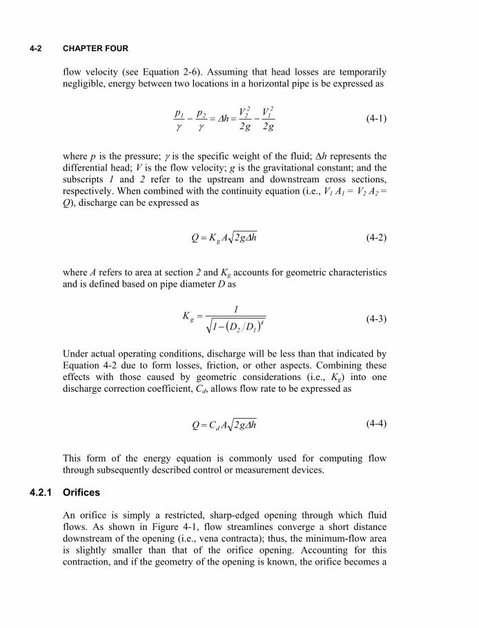
An orifice is simply a restricted, sharp-edged opening through which fluid flows. As shown in Figure 4-1, flow streamlines converge a short distance downstream of the opening (i.e., vena contracta); thus, the minimum-flow area is slightly smaller than that of the orifice opening. Accounting for this contraction, and if the geometry of the opening is known, the orifice becomes a
FLOW MEASUREMENT AND CONTROL 4-3
convenient and relatively inexpensive flow measurement device. The abrupt constriction of flow, however, simultaneously serves as the major limitation in their application. It is capable of causing a significant head loss and does not pass solids. The latter implies that it should not be used for wastewaters carrying significant solids concentrations because of potential clogging.
Vena contracta
D
FIGURE 4-1: Flow through an orifice meter
Discharge through an orifice can be expressed using Equation 4-4, in which A is the orifice area and the differential pressure head (i.e., ∆h) across the orifice is often determined using pressure transducers. The pressure that is lost across the orifice recovers to a small extent further downstream, but not to the previous upstream level. For example, at an orifice to pipe area ratio of 0.5, the permanent head loss is roughly 75% of the measured pressure differential.
The orifice discharge coefficient (i.e., Cd) corrects for the geometry of the contraction and energy losses through the opening. Generally speaking, the coefficient is relatively constant for Reynolds numbers, Re, greater than approximately 105, ranging from 0.6, for smaller ratios of orifice to pipe area to 0.9. Here, Re refers to that for flow through the orifice opening. At lower Reynolds numbers, coefficients vary more widely and depend on both the Re and the ratio of areas. Additional information, including standard specifications and corresponding coefficients, can be found in Brater et al. (1996) and numerous other fluid mechanics and hydraulic engineering references.
4.2.2 Venturi Meters
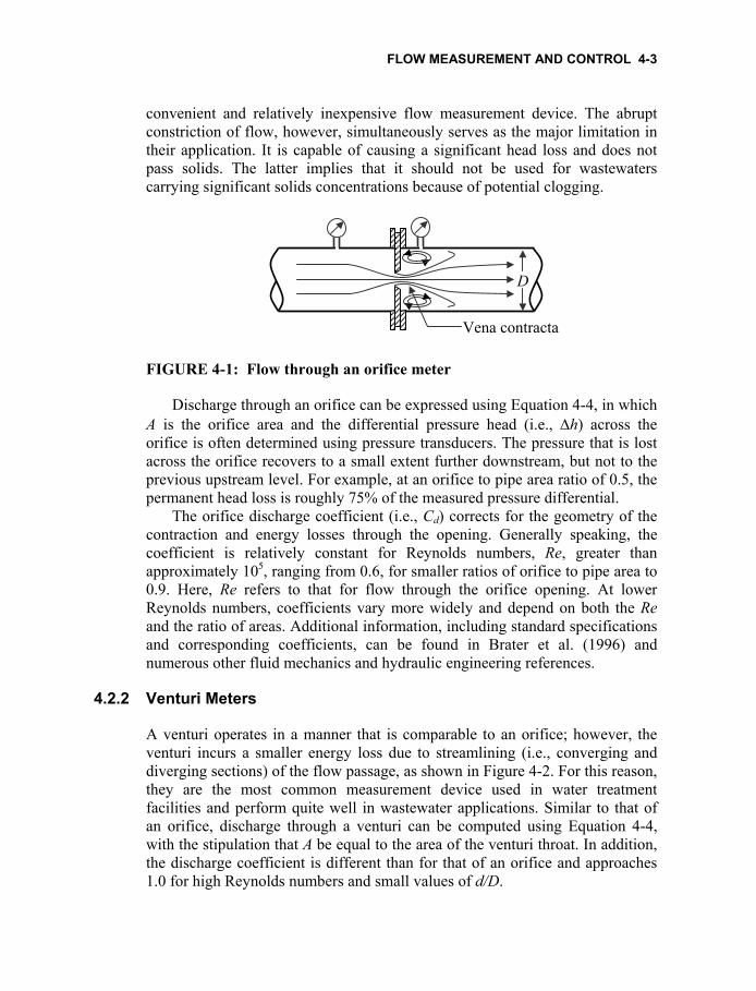
A venturi operates in a manner that is comparable to an orifice; however, the venturi incurs a smaller energy loss due to streamlining (i.e., converging and diverging sections) of the flow passage, as shown in Figure 4-2. For this reason, they are the most common measurement device used in water treatment facilities and perform quite well in wastewater applications. Similar to that of an orifice, discharge through a venturi can be computed using Equation 4-4, with the stipulation that A be equal to the area of the venturi throat. In addition, the discharge coefficient is different than for that of an orifice and approaches 1.0 for high Reynolds numbers and small values of d/D.
4-4 CHAPTER FOUR
d D
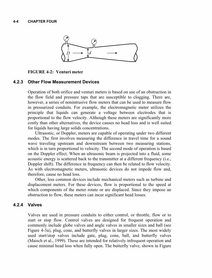
FIGURE 4-2: Venturi meter
4.2.3 Other Flow Measurement Devices
Operation of both orifice and venturi meters is based on use of an obstruction in the flow field and pressure taps that are susceptible to clogging. There are, however, a series of nonintrusive flow meters that can be used to measure flow in pressurized conduits. For example, the electromagnetic meter utilizes the principle that liquids can generate a voltage between electrodes that is proportional to the flow velocity. Although these meters are significantly more costly than other alternatives, the device causes no head loss and is well suited for liquids having large solids concentrations.
Ultrasonic, or Doppler, meters are capable of operating under two different modes. The first involves measuring the difference in travel time for a sound wave traveling upstream and downstream between two measuring stations, which is in turn proportional to velocity. The second mode of operation is based on the Doppler effect. When an ultrasonic beam is projected into a fluid, some acoustic energy is scattered back to the transmitter at a different frequency (i.e., Doppler shift). The difference in frequency can then be related to flow velocity. As with electromagnetic meters, ultrasonic devices do not impede flow and, therefore, cause no head loss.
Other, less common devices include mechanical meters such as turbine and displacement meters. For these devices, flow is proportional to the speed at which components of the meter rotate or are displaced. Since they impose an obstruction to flow, these meters can incur significant head losses.
4.2.4 Valves
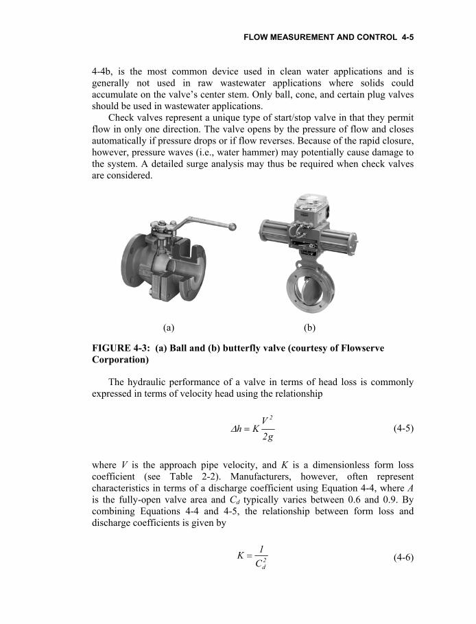
Valves are used in pressure conduits to either control, or throttle, flow or to start or stop flow. Control valves are designed for frequent operation and commonly include globe valves and angle valves in smaller sizes and ball (see Figure 4-3a), plug, cone, and butterfly valves in larger sizes. The most widely used start/stop valves include gate, plug, cone, ball, and butterfly valves (Maisch et al., 1999). These are intended for relatively infrequent operation and cause minimal head loss when fully open. The butterfly valve, shown in Figure
FLOW MEASUREMENT AND CONTROL 4-5
4-4b, is the most common device used in clean water applications and is generally not used in raw wastewater applications where solids could accumulate on the valve’s center stem. Only ball, cone, and certain plug valves should be used in wastewater applications.
Check valves represent a unique type of start/stop valve in that they permit flow in only one direction. The valve opens by the pressure of flow and closes automatically if pressure drops or if flow reverses. Because of the rapid closure, however, pressure waves (i.e., water hammer) may potentially cause damage to the system. A detailed surge analysis may thus be required when check valves are considered.
(a) (b)
FIGURE 4-3: (a) Ball and (b) butterfly valve (courtesy of Flowserve Corporation)
The hydraulic performance of a valve in terms of head loss is commonly expressed in terms of velocity head using the relationship
g2V
Kh2
=∆ (4-5) where V is the approach pipe velocity, and K is a dimensionless form loss coefficient (see Table 2-2). Manufacturers, however, often represent characteristics in terms of a discharge coefficient using Equation 4-4, where A is the fully-open valve area and Cd typically varies between 0.6 and 0.9. By combining Equations 4-4 and 4-5, the relationship between form loss and discharge coefficients is given by
2dC
1K = (4-6)
4-6 CHAPTER FOUR
In addition, valve performance can be expressed in terms of a dimensionless valve coefficient, Cv, introduced by the valve industry. The coefficient essentially represents the flow in gallons per minute (gpm) of 60° F water that can pass through the valve at a pressure differential of 1 lb/in2. Mathematically,
KDLC
2
1v = (4-7) where L1 is equal to 4,298 in U.S. customary units and 2.92 in S.I. units and D is the approach pipe diameter. Cv is related to discharge by
(4-8) pCLQ v2 ∆= The variable L2 is a constant equal to 1.0 if Q is in gpm and differential pressure across the valve, ∆p, is in psi and equal to 0.381 if Q is in m3/s and ∆p is in kPa (Sanks, 1989). Valves are often listed by manufacturers according to the Cv value; thus for a given flow rate, Equation 4-8 can be used to compute the required Cv, which can be used in selecting appropriate valve size.
4.2.5 Flow Manifolds
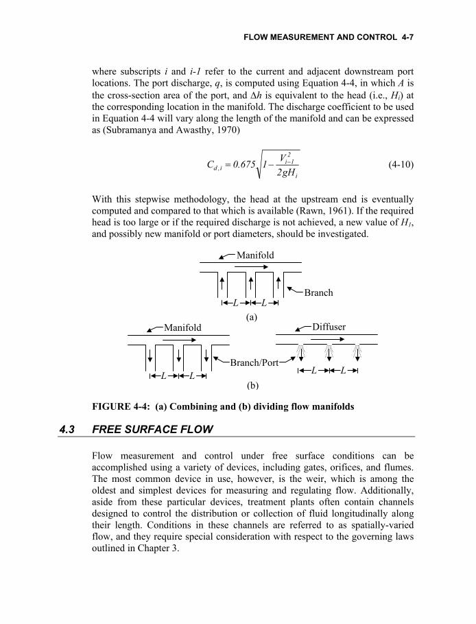
Manifolds are pipes that branch into other pipes to either combine or divide flow as shown in Figure 4-4. In treatment plants, dividing-flow systems are the most common; they are often used in the rapid dilution of wastewater effluent to water bodies and the distribution of flow uniformly across the width of one or more treatment units. Diffusion is accomplished either by separate branching pipes or by a series of ports cut in a manifold. In both cases, the flow from each branch will vary slightly as head changes along the length of the manifold. Thus, even though uniform flow distribution is the objective, a small degree of variation is likely and is normally acceptable.
The analysis of a dividing-flow system begins at the downstream end of the manifold with an assumed downstream energy, H1. With assumed manifold and port diameters, an energy balance then proceeds upstream in a stepwise fashion, accounting for corresponding elevation changes and friction losses in the manifold. In determining losses using an appropriate resistance equation (e.g., Darcy-Weisbach equation), the mean manifold velocity at a particular location can be obtained via continuity, expressed as
4DqVV 2
i1ii π+= − (4-9)
FLOW MEASUREMENT AND CONTROL 4-7
where subscripts i and i-1 refer to the current and adjacent downstream port locations. The port discharge, q, is computed using Equation 4-4, in which A is the cross-section area of the port, and ∆h is equivalent to the head (i.e., Hi) at the corresponding location in the manifold. The discharge coefficient to be used in Equation 4-4 will vary along the length of the manifold and can be expressed as (Subramanya and Awasthy, 1970)
i
21i
i ,d gH2V1675.0C −−= (4-10)
With this stepwise methodology, the head at the upstream end is eventually computed and compared to that which is available (Rawn, 1961). If the required head is too large or if the required discharge is not achieved, a new value of H1, and possibly new manifold or port diameters, should be investigated.
Branch
Manifold
L L
Branch/PortLL
Diffuser(a)
L L
Manifold (b)
FIGURE 4-4: (a) Combining and (b) dividing flow manifolds
4.3 FREE SURFACE FLOW
Flow measurement and control under free surface conditions can be accomplished using a variety of devices, including gates, orifices, and flumes. The most common device in use, however, is the weir, which is among the oldest and simplest devices for measuring and regulating flow. Additionally, aside from these particular devices, treatment plants often contain channels designed to control the distribution or collection of fluid longitudinally along their length. Conditions in these channels are referred to as spatially-varied flow, and they require special consideration with respect to the governing laws outlined in Chapter 3.
4-8 CHAPTER FOUR
4.3.1 Weirs
A weir is essentially any device placed perpendicular, or parallel in the case of a side weir, to flow in order create a unique relationship between depth (head) and discharge. The head-discharge relationship then allows for quick evaluation of flow rate or serves as a hydraulic control point for subsequent gradually-varied flow computations. Sharp-crested and broad-crested are the most widely used types of weirs used in treatment plant operation. The continued popularity of weirs is primarily due to the ease with which they can be constructed and the extensive set of previous experimental results derived for various weirs. Their use should, however, be restricted to cases in which liquid streams do not contain considerable quantities of settleable solids (e.g., raw wastewater) because of a tendency for deposition behind the weir. In addition, the designer should be aware of the potentially large head losses introduced by weirs and make adjustments to overall plant hydraulics if needed.
4.3.1.1 Sharp-Crested Weirs
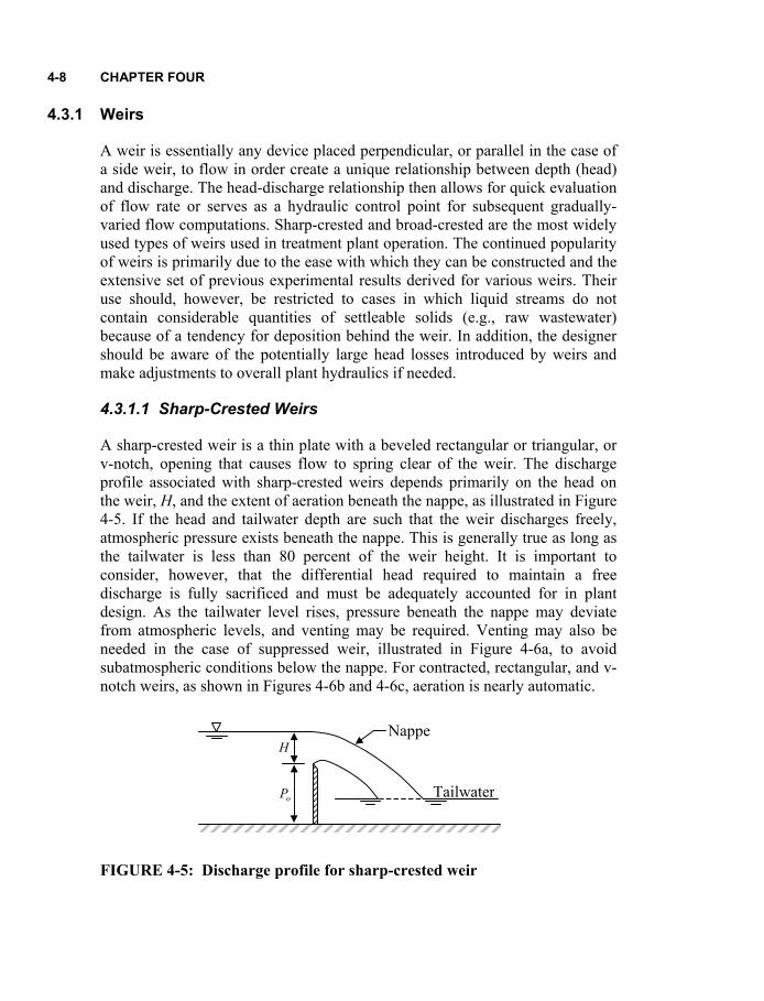
A sharp-crested weir is a thin plate with a beveled rectangular or triangular, or v-notch, opening that causes flow to spring clear of the weir. The discharge profile associated with sharp-crested weirs depends primarily on the head on the weir, H, and the extent of aeration beneath the nappe, as illustrated in Figure 4-5. If the head and tailwater depth are such that the weir discharges freely, atmospheric pressure exists beneath the nappe. This is generally true as long as the tailwater is less than 80 percent of the weir height. It is important to consider, however, that the differential head required to maintain a free discharge is fully sacrificed and must be adequately accounted for in plant design. As the tailwater level rises, pressure beneath the nappe may deviate from atmospheric levels, and venting may be required. Venting may also be needed in the case of suppressed weir, illustrated in Figure 4-6a, to avoid subatmospheric conditions below the nappe. For contracted, rectangular, and v-notch weirs, as shown in Figures 4-6b and 4-6c, aeration is nearly automatic.
HNappe
oP Tailwater
FIGURE 4-5: Discharge profile for sharp-crested weir
FLOW MEASUREMENT AND CONTROL 4-9
Development of head-discharge relationship for sharp crested weirs begins by neglecting frictional and vertical contraction effects and by assuming the space beneath the nappe is adequately aerated. For a suppressed, rectangular weir and with these assumptions, discharge can be expressed as
23d LHg2
32CQ = (4-11)
where L is the crest length, and Cd is a discharge coefficient used to correct for the previous assumptions and is equivalent to (Henderson, 1966)
od P
H075.0611.0C += (4-12) For most applications, the value of Cd will approach 0.62; thus, Equation 4-11 can be written in its more common form,
(4-13) 231LHCQ =
where C1 is a constant equal to 3.33 in U.S. customary units and 1.84 in S.I. units. If the weir is contracted (i.e., Figure 4-6b), the same relationship applies, but L should be replaced by an effective crest length, L′, expressed as
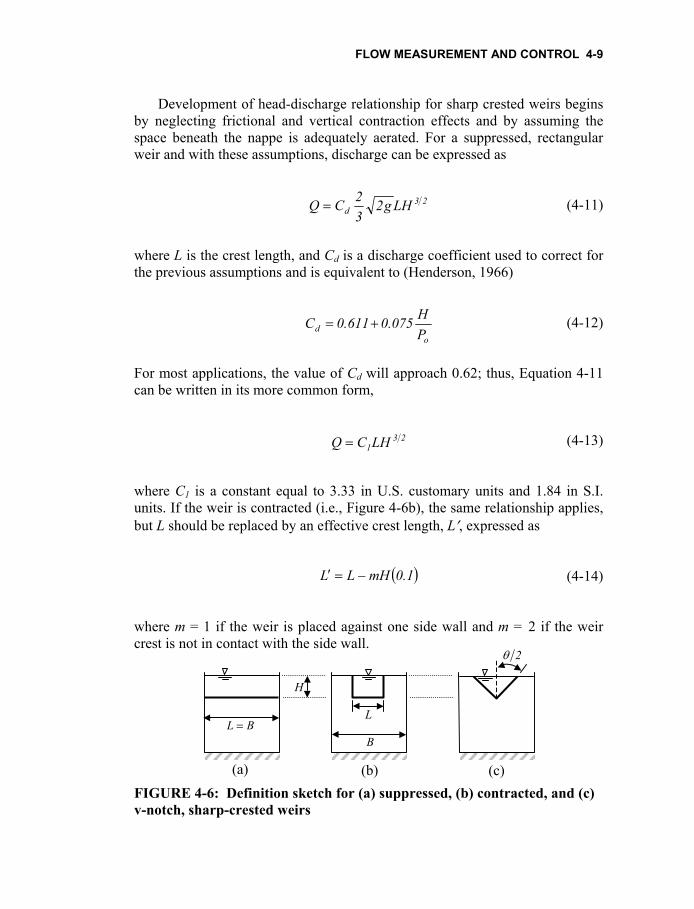
( )1.0mHLL −=′ (4-14) where m = 1 if the weir is placed against one side wall and m = 2 if the weir crest is not in contact with the side wall.
H
BL =L
2θ
B
(a) (b) (c) FIGURE 4-6: Definition sketch for (a) suppressed, (b) contracted, and (c) v-notch, sharp-crested weirs
4-10 CHAPTER FOUR
V-notch weirs, such as that shown in Figure 4-6c, are well suited for lower flow rates, but tend to function well over a very wide range of flows. The corresponding head-discharge relationship for these weirs is
25d Hg2
2tanC
158Q θ
= (4-15) where θ is the weir angle. For θ = 90°, the most commonly used v-notch angle, Cd assumes a value of approximately 0.585. Thus, Equation 4-15 can be rewritten as
(4-16) 252HCQ =
where C2 is equal to 2.49 in U.S. customary units and 1.37 in S.I. units. For other angles between 20° and 120°, and as long as H is at least 2 in (50 mm), using Cd = 0.58 in Equation 4-15 is normally acceptable for engineering calculations (Potter and Wiggert, 2002).
In addition, saw-toothed weirs, consisting of many small v-notch weirs are common in effluent structures (clarifiers) at wastewater treatment facilities. In this case, total discharge is divided among the total number of individual v-notch weirs.
Note that if the ratio of head to sharp-crested weir height (i.e., H/Po) exceeds five, the upstream velocity head may be appreciable and it should be included as part of the head on the weir. If H/Po > 15, the weir essentially becomes a sill, and discharge can be evaluated by assuming that the head is equivalent to the critical depth of flow (Chaudhry, 1993). In addition, be aware that if the tailwater increases above the height of the weir crest, the weir becomes submerged, or drowned, and the previous relationships are inadequate. In this case, the discharge can be best approximated by (Villamonte, 1947)
385.05.1
1
2
HH1QQ
⎥⎥⎦
⎤
⎢⎢⎣
⎡⎟⎟⎠
⎞⎜⎜⎝
⎛−′= (4-17)
where Q′ is the discharge for the case of a free flowing (i.e., unsubmerged) weir and H1 and H2 refer to upstream and downstream head on the weir, respectively. Equation 4-17 applies to all sharp-crested weirs, including those that are rectangular and v-notch in shape.
FLOW MEASUREMENT AND CONTROL 4-11
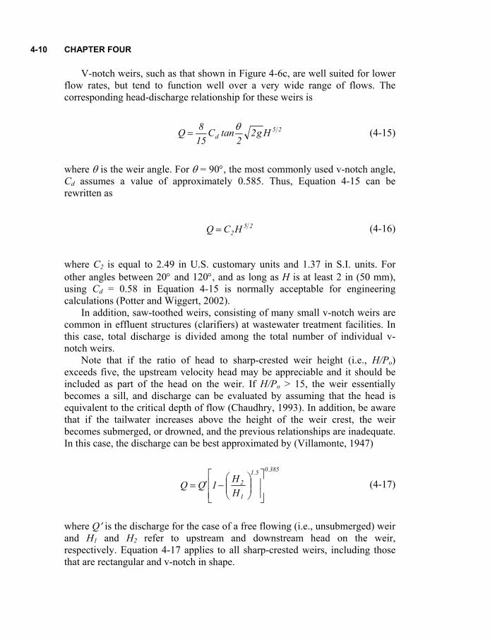
4.3.1.2 Broad-Crested Weirs
Broad-crested weirs have a long, rectangular-shaped profile. The crest is designed such that parallel flow and critical depth occur at some point along the crest, as shown in Figure 4-7.
H
oP
cy
EGL
FIGURE 4-7: Broad-crested weir
Using critical flow principles, and noting that yc = 1.5 × H, where H includes upstream velocity head, discharge can be expressed as
2323
d BHg32CQ ⎟⎠⎞
⎜⎝⎛= (4-18)
where B is channel width. The corresponding discharge correction factor can be estimated by (Chow, 1988)
( ) 5.0o
d PH165.0C
+= (4-19)
For proper operation of a broad-crested weir, flow conditions are restricted to 0.08 < Ho/L < 0.33, where Ho is the upstream depth above the crest, and L is length of the weir. In addition, tailwater elevations should be less than 0.8H above the weir crest to ensure free flowing discharges (Henderson, 1966).
4.3.2 Gates
Underflow gates, such as sluice (see Figure 4-8), drum, and radial (e.g., Tainter) gates, can be used simultaneously to control flow and provide for convenient flow measurement in channels. In these cases, discharge can be expressed using a relationship that is similar to Equation 4-4,
(4-20) 1d gy2BaCQ =
4-12 CHAPTER FOUR
where y1 is the upstream depth. For a free discharge, Cd can be expressed as
( )1c
cd yaC1
CC+
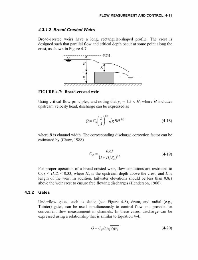
= (4-21) in which the contraction coefficient, Cc, assumes a value of 0.61 for a/E1 < 0.5 (Chadwick and Morfett, 1986). Note that if the downstream jet is submerged, Cd becomes a function of the downstream depth, y2, as well.
FIGURE 4-8: Flow through a sluice gate
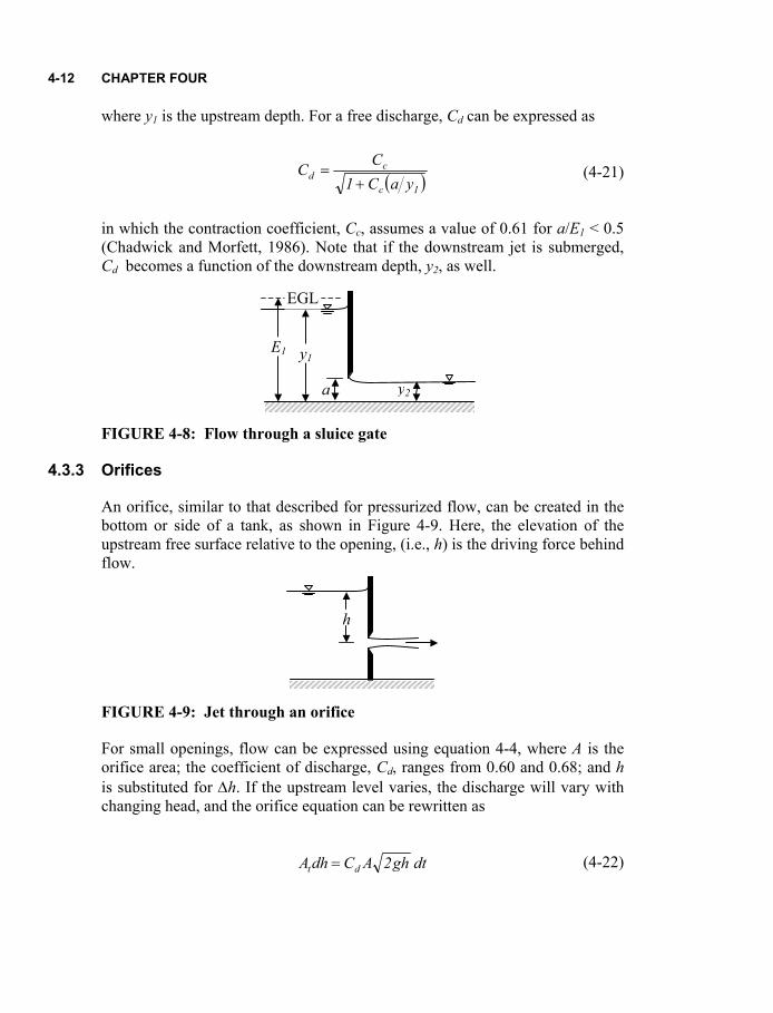
4.3.3 Orifices
An orifice, similar to that described for pressurized flow, can be created in the bottom or side of a tank, as shown in Figure 4-9. Here, the elevation of the upstream free surface relative to the opening, (i.e., h) is the driving force behind flow.
h
y1
a
E1
EGL
y2
FIGURE 4-9: Jet through an orifice
For small openings, flow can be expressed using equation 4-4, where A is the orifice area; the coefficient of discharge, Cd, ranges from 0.60 and 0.68; and h is substituted for ∆h. If the upstream level varies, the discharge will vary with changing head, and the orifice equation can be rewritten as
(4-22) dt gh2ACdhA dt =
FLOW MEASUREMENT AND CONTROL 4-13
where At is the cross-sectional area of the tank. Also note that if a constant inflow to the tank (i.e., Qi) simultaneously occurs, a quantity equal to Qidt should be subtracted from the right-hand side of Equation 4-22.
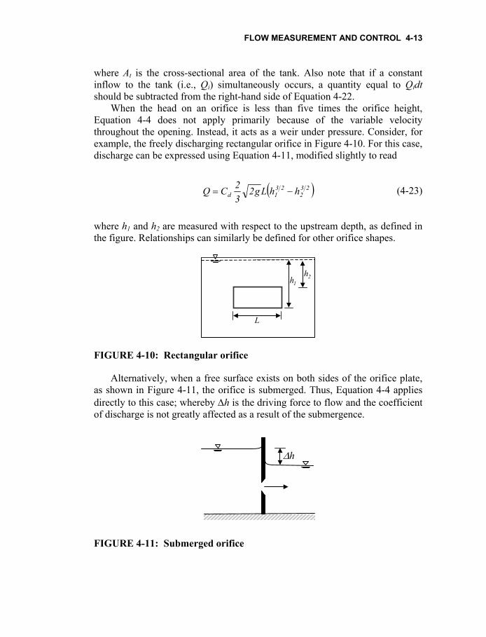
When the head on an orifice is less than five times the orifice height, Equation 4-4 does not apply primarily because of the variable velocity throughout the opening. Instead, it acts as a weir under pressure. Consider, for example, the freely discharging rectangular orifice in Figure 4-10. For this case, discharge can be expressed using Equation 4-11, modified slightly to read
( )232
231d hhLg2
32CQ −= (4-23)
where h1 and h2 are measured with respect to the upstream depth, as defined in the figure. Relationships can similarly be defined for other orifice shapes.
FIGURE 4-10: Rectangular orifice
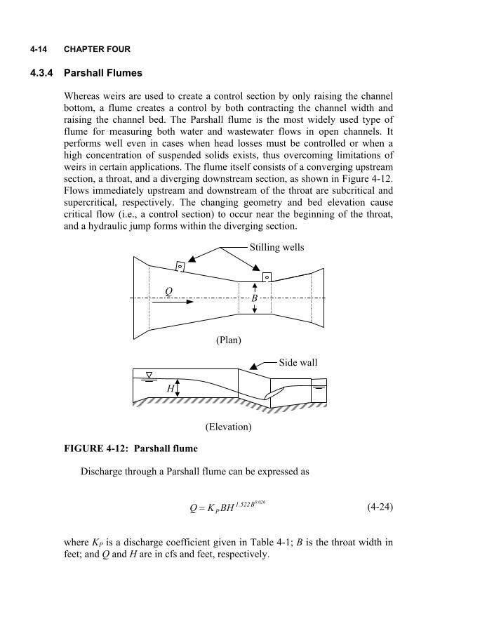
Alternatively, when a free surface exists on both sides of the orifice plate, as shown in Figure 4-11, the orifice is submerged. Thus, Equation 4-4 applies directly to this case; whereby ∆h is the driving force to flow and the coefficient of discharge is not greatly affected as a result of the submergence.
∆h
2h
L
1h
FIGURE 4-11: Submerged orifice
4-14 CHAPTER FOUR
4.3.4 Parshall Flumes
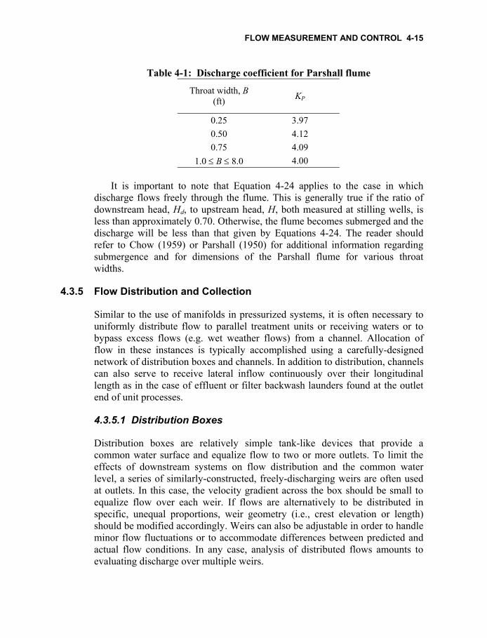
Whereas weirs are used to create a control section by only raising the channel bottom, a flume creates a control by both contracting the channel width and raising the channel bed. The Parshall flume is the most widely used type of flume for measuring both water and wastewater flows in open channels. It performs well even in cases when head losses must be controlled or when a high concentration of suspended solids exists, thus overcoming limitations of weirs in certain applications. The flume itself consists of a converging upstream section, a throat, and a diverging downstream section, as shown in Figure 4-12. Flows immediately upstream and downstream of the throat are subcritical and supercritical, respectively. The changing geometry and bed elevation cause critical flow (i.e., a control section) to occur near the beginning of the throat, and a hydraulic jump forms within the diverging section.
B
Stilling wells
(Plan)
Q
Side wall
H
(Elevation)
FIGURE 4-12: Parshall flume
Discharge through a Parshall flume can be expressed as
(4-24) 026.0B522.1P BHKQ =
where KP is a discharge coefficient given in Table 4-1; B is the throat width in feet; and Q and H are in cfs and feet, respectively.
FLOW MEASUREMENT AND CONTROL 4-15
Table 4-1: Discharge coefficient for Parshall flume
Throat width, B (ft) KP
0.25 3.97 0.50 4.12 0.75 4.09
1.0 ≤ B ≤ 8.0 4.00
It is important to note that Equation 4-24 applies to the case in which discharge flows freely through the flume. This is generally true if the ratio of downstream head, Hd, to upstream head, H, both measured at stilling wells, is less than approximately 0.70. Otherwise, the flume becomes submerged and the discharge will be less than that given by Equations 4-24. The reader should refer to Chow (1959) or Parshall (1950) for additional information regarding submergence and for dimensions of the Parshall flume for various throat widths.
4.3.5 Flow Distribution and Collection
Similar to the use of manifolds in pressurized systems, it is often necessary to uniformly distribute flow to parallel treatment units or receiving waters or to bypass excess flows (e.g. wet weather flows) from a channel. Allocation of flow in these instances is typically accomplished using a carefully-designed network of distribution boxes and channels. In addition to distribution, channels can also serve to receive lateral inflow continuously over their longitudinal length as in the case of effluent or filter backwash launders found at the outlet end of unit processes.
4.3.5.1 Distribution Boxes
Distribution boxes are relatively simple tank-like devices that provide a common water surface and equalize flow to two or more outlets. To limit the effects of downstream systems on flow distribution and the common water level, a series of similarly-constructed, freely-discharging weirs are often used at outlets. In this case, the velocity gradient across the box should be small to equalize flow over each weir. If flows are alternatively to be distributed in specific, unequal proportions, weir geometry (i.e., crest elevation or length) should be modified accordingly. Weirs can also be adjustable in order to handle minor flow fluctuations or to accommodate differences between predicted and actual flow conditions. In any case, analysis of distributed flows amounts to evaluating discharge over multiple weirs.
4-16 CHAPTER FOUR
4.3.5.2 Distribution Channels
The design and analysis of distribution channels is slightly more complex than that of the distribution box since a portion of discharge leaves the channel along its longitudinal length. Lateral flows are typically accomplished using side-discharge weirs or gates. In either case, flow should be freely discharged (i.e., unsubmerged) in order to minimize the effects on flow within the main channel caused by conditions at points of distribution. The analysis of distribution channels typically focuses on determination of lateral outflow. The evaluation of channel depth (i.e., water surface profile) is generally of secondary importance since side weirs or gates are short relative to the channel length; therefore, water-level changes are typically too small to be decisive criteria in design and analysis.
Flow through distribution channels is described as spatially-varied. Since the longitudinal velocity, and thus the corresponding momentum flux, of lateral flow is unknown and since the outflow represents a local disturbance, energy principles are used more often than momentum concepts to develop a corresponding discharge relationship. Assuming So = Sf = 0, a reasonable assumption given the length of a typical side weir, the spatially-varied flow equation can be written as ( )( )
2
2
Fr1dxdQgAQ
dxdy
−−
= (4-25)
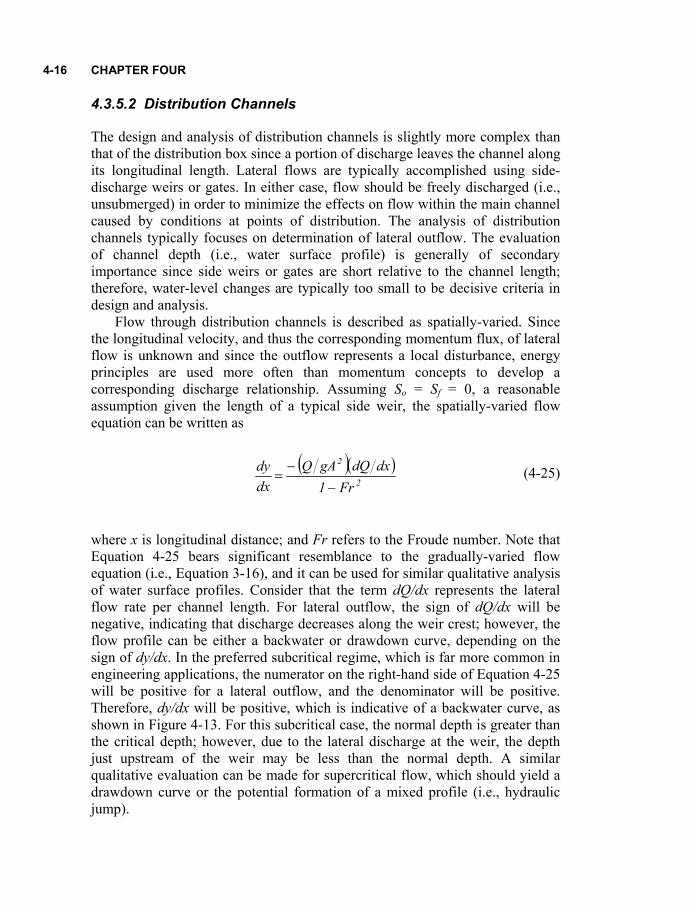
where x is longitudinal distance; and Fr refers to the Froude number. Note that Equation 4-25 bears significant resemblance to the gradually-varied flow equation (i.e., Equation 3-16), and it can be used for similar qualitative analysis of water surface profiles. Consider that the term dQ/dx represents the lateral flow rate per channel length. For lateral outflow, the sign of dQ/dx will be negative, indicating that discharge decreases along the weir crest; however, the flow profile can be either a backwater or drawdown curve, depending on the sign of dy/dx. In the preferred subcritical regime, which is far more common in engineering applications, the numerator on the right-hand side of Equation 4-25 will be positive for a lateral outflow, and the denominator will be positive. Therefore, dy/dx will be positive, which is indicative of a backwater curve, as shown in Figure 4-13. For this subcritical case, the normal depth is greater than the critical depth; however, due to the lateral discharge at the weir, the depth just upstream of the weir may be less than the normal depth. A similar qualitative evaluation can be made for supercritical flow, which should yield a drawdown curve or the potential formation of a mixed profile (i.e., hydraulic jump).
FLOW MEASUREMENT AND CONTROL 4-17
L
oP1y x 2y
FIGURE 4-13: Spatially-varied flow at a side-discharge weir
Application of Equation 4-25 for the case of decreasing channel discharge requires a suitable depth-discharge relationship. For side weirs,
( ) 23od Pyg2C
dxdQ
−=− (4-26) where Po is the weir height, and the discharge coefficient, Cd, is often taken as 0.42 for a sharp-crested side weir. Borghei et al. (2003), however, reviewed previously proposed formulas for Cd and indicated the coefficient for subcritical flow is better estimated as
⎟⎟⎠
⎞⎜⎜⎝
⎛+−−=
BL06.0
yP3.0Fr48.07.0
32C
1
o1d (4-27)
where Fr1 and y1 refer to the Froude number and depth at the upstream end of the weir. In addition to the depth-discharge relation, conservation of energy can be used to define the discharge at any section and is written here as
( )yEg2ByQ −= (4-28) where E is specific energy, and B is the channel width. Substituting Equations 4-26 and 4-28 into 4-25 and integrating yields (De Marchi, 1934)
ZPEyEsin3
PyyE
PEP3E2
BxC
o
1
oo
od +−−
−−−
−−
= − (4-29)
4-18 CHAPTER FOUR
where Z is a constant of integration. This expression can be solved within the limits of the weir to obtain crest length for a given discharge or to indirectly determine discharge for a given length.
The De Marchi equation (i.e., Equation 4-29) is the most commonly used method for evaluating distributed channel flows over side weirs. However, the reader is also referred to Hager (1987), who developed an alternative discharge equation that includes the effects of lateral outflow angle and channel width; to Muslu (2001), who describes flow characteristics using dimensionless terms and provides a numerical solution approach to the side weir problem; and to El-Khashab and Smith (1976), Uyumaz and Muslu (1985), and Gisonni and Hager (1997), who considered the lateral outflow problem for trapezoidal, circular, and U-shaped channels, respectively.
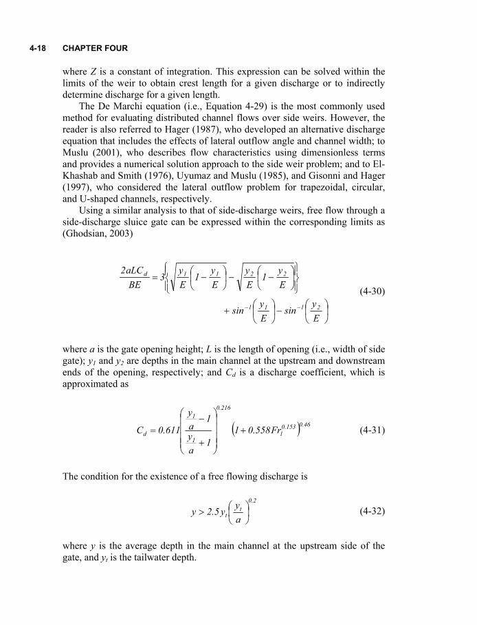
Using a similar analysis to that of side-discharge weirs, free flow through a side-discharge sluice gate can be expressed within the corresponding limits as (Ghodsian, 2003)
⎟⎠
⎞⎜⎝
⎛−⎟⎠
⎞⎜⎝
⎛+
⎪⎭
⎪⎬⎫
⎪⎩
⎪⎨⎧
⎟⎠
⎞⎜⎝
⎛−−⎟
⎠
⎞⎜⎝
⎛−=
−−
Ey
sinEy
sin
Ey
1Ey
Ey
1Ey
3BE
aLC2
2111
2211d
(4-30) where a is the gate opening height; L is the length of opening (i.e., width of side gate); y1 and y2 are depths in the main channel at the upstream and downstream ends of the opening, respectively; and Cd is a discharge coefficient, which is approximated as
(4-31) ( ) 46.0153.01
216.0
1
1
d Fr558.011
ay
1ay
611.0C +⎟⎟⎟⎟
⎠
⎞
⎜⎜⎜⎜
⎝
⎛
+
−=
The condition for the existence of a free flowing discharge is 2.0
tt a
yy5.2y ⎟⎠⎞
⎜⎝⎛> (4-32)
where y is the average depth in the main channel at the upstream side of the gate, and yt is the tailwater depth.
FLOW MEASUREMENT AND CONTROL 4-19
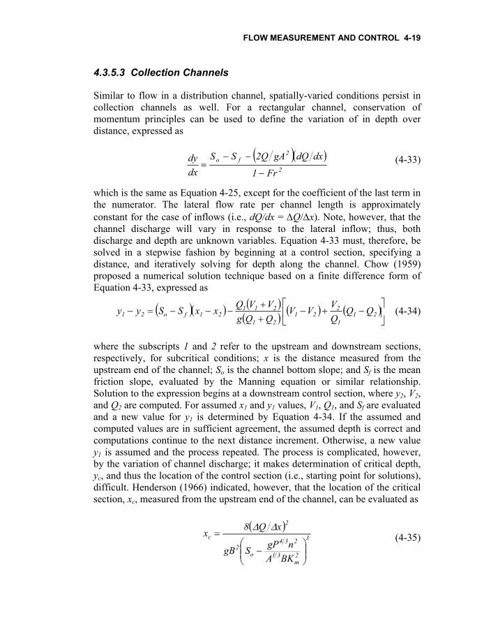
4.3.5.3 Collection Channels
Similar to flow in a distribution channel, spatially-varied conditions persist in collection channels as well. For a rectangular channel, conservation of momentum principles can be used to define the variation of in depth over distance, expressed as
( )( )2
2fo
Fr1
dxdQgAQ2SSdxdy
−
−−=
(4-33)
which is the same as Equation 4-25, except for the coefficient of the last term in the numerator. The lateral flow rate per channel length is approximately constant for the case of inflows (i.e., dQ/dx = ∆Q/∆x). Note, however, that the channel discharge will vary in response to the lateral inflow; thus, both discharge and depth are unknown variables. Equation 4-33 must, therefore, be solved in a stepwise fashion by beginning at a control section, specifying a distance, and iteratively solving for depth along the channel. Chow (1959) proposed a numerical solution technique based on a finite difference form of Equation 4-33, expressed as
(4-34) ( )( ) ( )( ) ( ) ( )⎥
⎦
⎤⎢⎣
⎡−+−
++
−−−=− 211
221
21
21121fo21 QQ
QVVV
QQgVVQxxSSyy
where the subscripts 1 and 2 refer to the upstream and downstream sections, respectively, for subcritical conditions; x is the distance measured from the upstream end of the channel; So is the channel bottom slope; and Sf is the mean friction slope, evaluated by the Manning equation or similar relationship. Solution to the expression begins at a downstream control section, where y2, V2, and Q2 are computed. For assumed x1 and y1 values, V1, Q1, and Sf are evaluated and a new value for y1 is determined by Equation 4-34. If the assumed and computed values are in sufficient agreement, the assumed depth is correct and computations continue to the next distance increment. Otherwise, a new value y1 is assumed and the process repeated. The process is complicated, however, by the variation of channel discharge; it makes determination of critical depth, yc, and thus the location of the control section (i.e., starting point for solutions), difficult. Henderson (1966) indicated, however, that the location of the critical section, xc, measured from the upstream end of the channel, can be evaluated as
( )3
2m
31
234
o2
2
c
BKAngPSgB
xQ8x
⎟⎟⎠
⎞⎜⎜⎝
⎛−
=∆∆
(4-35)
4-20 CHAPTER FOUR
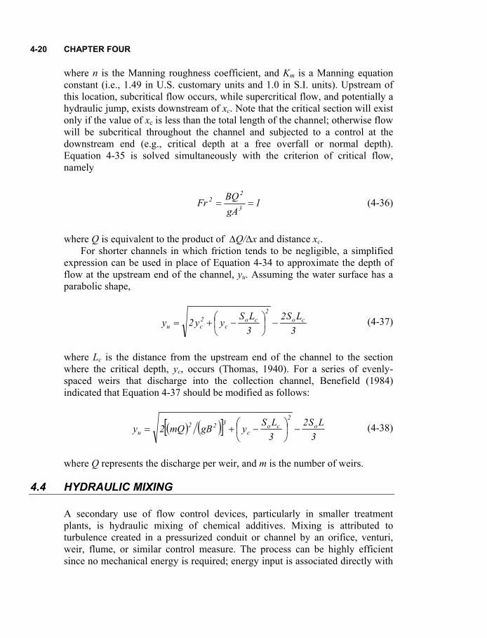
where n is the Manning roughness coefficient, and Km is a Manning equation constant (i.e., 1.49 in U.S. customary units and 1.0 in S.I. units). Upstream of this location, subcritical flow occurs, while supercritical flow, and potentially a hydraulic jump, exists downstream of xc. Note that the critical section will exist only if the value of xc is less than the total length of the channel; otherwise flow will be subcritical throughout the channel and subjected to a control at the downstream end (e.g., critical depth at a free overfall or normal depth). Equation 4-35 is solved simultaneously with the criterion of critical flow, namely
1gABQFr 3
22 == (4-36)
where Q is equivalent to the product of ∆Q/∆x and distance xc.
For shorter channels in which friction tends to be negligible, a simplified expression can be used in place of Equation 4-34 to approximate the depth of flow at the upstream end of the channel, yu. Assuming the water surface has a parabolic shape,
3LS2
3LSyy2y co
2co
c2cu −⎟
⎠⎞
⎜⎝⎛ −+= (4-37)
where Lc is the distance from the upstream end of the channel to the section where the critical depth, yc, occurs (Thomas, 1940). For a series of evenly-spaced weirs that discharge into the collection channel, Benefield (1984) indicated that Equation 4-37 should be modified as follows:
( ) ( )[ ]3
LS23LSygBmQ2y o
2co
c322
u −⎟⎠⎞
⎜⎝⎛ −+= (4-38)
where Q represents the discharge per weir, and m is the number of weirs.
4.4 HYDRAULIC MIXING
A secondary use of flow control devices, particularly in smaller treatment plants, is hydraulic mixing of chemical additives. Mixing is attributed to turbulence created in a pressurized conduit or channel by an orifice, venturi, weir, flume, or similar control measure. The process can be highly efficient since no mechanical energy is required; energy input is associated directly with
FLOW MEASUREMENT AND CONTROL 4-21
flow characteristics. The principal difficulty, however, is that energy varies with flow rate. Consider that during periods of low flow, sufficient energy may not be available to achieve sufficient mixing levels. One means to overcome this limitation is to vary the number hydraulic modules (e.g., venturi or flume) in operation at any one time to maintain relatively constant flows in those modules in operation.
The intensity of mixing, or degree of agitation, is typically expressed using the mean velocity gradient, G, defined as
∀=
µPG (4-39)
where P is power input; µ is dynamic, or absolute, viscosity; and ∀ is channel or tank volume. Power input can be computed by
(4-40) hQP γ= where h is the differential head over the device being considered. As an example, the energy associated with water flowing over a weir with an effective fall of 1 ft (30 cm) typically yields an intensity of approximately 1,000 sec-1 at 20° (AWWA/ASCE, 1990). Note that that detention time is not explicitly addressed in Equation 4-35, but it must be considered for most rapid mixing systems. A more detailed discussion of the hydraulic aspects of mixing can be found in Chapter 6.
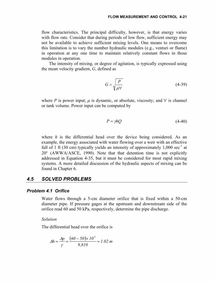
4.5 SOLVED PROBLEMS
Problem 4.1 Orifice Water flows through a 5-cm diameter orifice that is fixed within a 50-cm diameter pipe. If pressure gages at the upstream and downstream side of the orifice read 60 and 50 kPa, respectively, determine the pipe discharge.
Solution
The differential head over the orifice is
( ) m 02.1810,9
105060ph3
=×−
==γ∆∆
4-22 CHAPTER FOUR
Assuming a discharge coefficient of 0.6 (i.e., large Re and small d/D), Equation 4-4 yields
( ) ( ) sm 005.002.181.92405.06.0Q 3
2
=××⎟⎟⎠
⎞⎜⎜⎝
⎛=
π
For this discharge, velocity (i.e., Q/A) is computed as 2.68 m/s and the corresponding Reynolds number is approximately
( )( ) 56 1034.1
1005.068.2VDRe ×=== −υ
Thus, the Cd = 0.6 was a reasonable assumption and the discharge is correct.
Problem 4.2 Venturi For Problem 4.1, how would the resulting discharge change if a venturi was used instead of an orifice? Assume the same differential head exists.
Solution
Assuming a discharge coefficient of 1.0, flow is computed as
( ) ( ) sm 009.002.181.92405.00.1Q 3
2
=××⎟⎟⎠
⎞⎜⎜⎝
⎛=
π
which is nearly double that of the orifice. Note that if discharge was the same as that determined in Problem 4.1, the associated differential head would be
( ) ( ) ( )m 33.0
405.081.920.1
005.0h 222
2
=
⎟⎟⎠
⎞⎜⎜⎝
⎛×
=π
∆
or approximately one-third of that for the orifice, demonstrating the difference in head loss experienced by the two meters.
Problem 4.3 Valve Determine the required valve coefficient to be used in selecting a control valve for a 6-in diameter pipe carrying 500 gpm with a maximum pressure differential of 5 psi.
FLOW MEASUREMENT AND CONTROL 4-23
Solution
Rearranging Equation 4-8,
6.2235
500Cv ==
This dimensionless valve coefficient can be used with manufacturers’ tables to select the appropriate valve size. Seldom will the exact value be listed; more typically the required Cv will fall between available valve sizes. In these cases, the next larger available size should be selected.
Problem 4.4 Valve Assume that for Problem 4.3, the valve selected has a Cv value of 720. Evaluate the corresponding head loss that is associated with the valve.
Solution
From Equation 4-7, the form loss and valve coefficients are related by
( ) 23.2720126298,4K
22
=⎟⎟⎠
⎞⎜⎜⎝
⎛×=
which can be compared to those listed in Table 2-2. The corresponding velocity in the approach pipe is evaluated as 5.65 m/s (i.e., Q/A), so that the head loss is expressed as
( ) m 15.12.322
65.523.2g2
VK22
=×
×=
Problem 4.5 Pipe manifold Effluent is to be discharged through a diffuser and into a lake at a rate of 15 cfs. The 1.5-ft diameter, PVC diffuser is 105-ft long and has sharp-edged ports spaced at 7-ft intervals. If the available head at the upstream end of the 250-ft long, 1.5-ft diameter supply pipe that feeds the diffuser is 25 ft, determine the diameter of ports to be used. Assume that elevation changes are negligible.
Solution
The number of ports (i.e., N) is equal to the total spacing divided by the port spacing, or 105/7 = 15 ports. The head at the most upstream port in the diffuser
4-24 CHAPTER FOUR
is found by subtracting the head loss in the 250-ft long supply line from the available head at the plant. Assuming ν = 1.2 × 10⁻⁵ ft2/s and ks = 5 × 10⁻⁶ ft for the PVC pipe,
( )( )( )( )
65 1006.1
5.1102.1154
DQ4VDRe ×=
×=== −ππνν
The Darcy-Weisbach friction factor can be computed using the Swamee-Jain equation (i.e., Equation 2-16), expressed as
( )( ) ( )
012.0
1006.174.5
5.17.3105ln
325.1f 2
9.06
6=
⎥⎥⎦
⎤
⎢⎢⎣
⎡
⎟⎟⎠
⎞⎜⎜⎝
⎛
×+
×=
−
Then the head at the end of the supply line, or the most upstream port in diffuser, is
( )( )( ) ( )( ) ( )
ft 8.222.325.1
815250012.025gD8fLQHhHH 25
2
25
2
plantfplantN =−=−=−=ππ
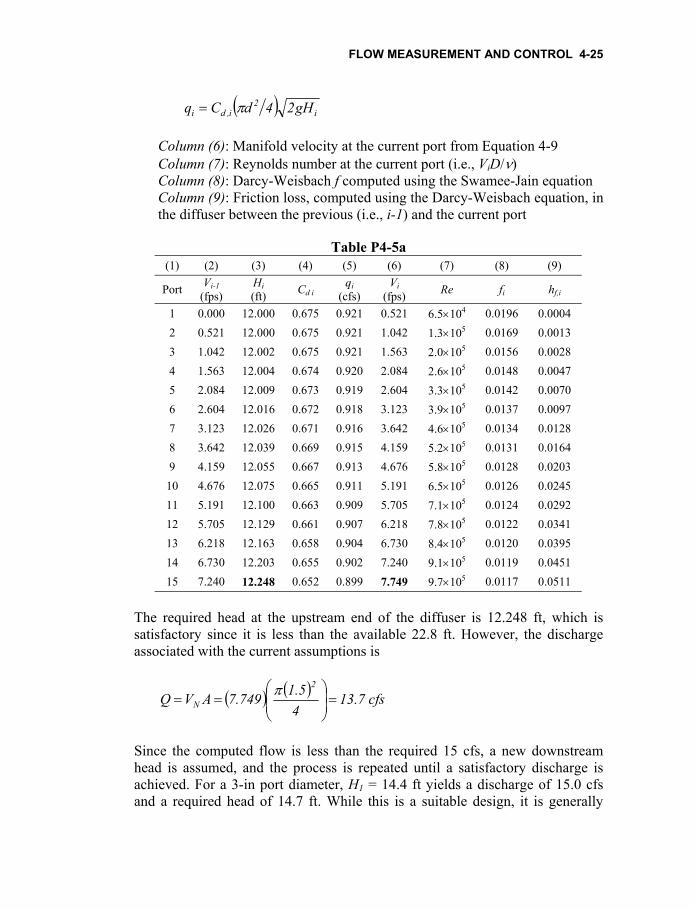
The analysis proceeds by finding the head at the downstream end of the diffuser that yields the desired discharge, then evaluating whether the head at the Nth port is less than or equal to that which is available. Table P4-5a summarizes the first iteration, in which a port diameter of 3 in is assumed. In addition, a downstream head (i.e., H1) of 12 ft is initially assumed. Specific entries in the table are as follows:
Columns (1): Port identification number, where i=1 is farthest downstream and i=N=15 is the most upstream port Column (2): Diffuser velocity at the downstream end is zero (i.e., dead end). For remaining rows, values are equal to the previous row of Column 6 Column (3): Head at the first port is 12 ft. Remaining values are computed using values in the previous row from Columns 3 and 9 as follows: i,fi 1i hHH +=+ Column (4): The discharge coefficient, computed using Equation 4-10, which is equal to 0.675 for the first port Column (5): Port discharge is computed using Equation 4-4, written as
FLOW MEASUREMENT AND CONTROL 4-25
( ) i2
i,di gH24dCq π= Column (6): Manifold velocity at the current port from Equation 4-9 Column (7): Reynolds number at the current port (i.e., ViD/ν) Column (8): Darcy-Weisbach f computed using the Swamee-Jain equation Column (9): Friction loss, computed using the Darcy-Weisbach equation, in the diffuser between the previous (i.e., i-1) and the current port
The required head at the upstream end of the diffuser is 12.248 ft, which is satisfactory since it is less than the available 22.8 ft. However, the discharge associated with the current assumptions is
( ) ( ) cfs 7.1345.1749.7AVQ
2
N =⎟⎟⎠
⎞⎜⎜⎝
⎛==
π
Since the computed flow is less than the required 15 cfs, a new downstream head is assumed, and the process is repeated until a satisfactory discharge is achieved. For a 3-in port diameter, H1 = 14.4 ft yields a discharge of 15.0 cfs and a required head of 14.7 ft. While this is a suitable design, it is generally
4-26 CHAPTER FOUR
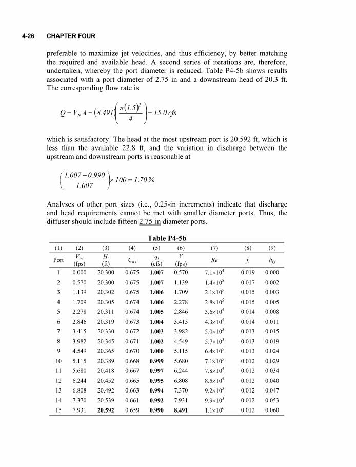
preferable to maximize jet velocities, and thus efficiency, by better matching the required and available head. A second series of iterations are, therefore, undertaken, whereby the port diameter is reduced. Table P4-5b shows results associated with a port diameter of 2.75 in and a downstream head of 20.3 ft. The corresponding flow rate is
( ) ( ) cfs 0.1545.1491.8AVQ
2
N =⎟⎟⎠
⎞⎜⎜⎝
⎛==
π
which is satisfactory. The head at the most upstream port is 20.592 ft, which is less than the available 22.8 ft, and the variation in discharge between the upstream and downstream ports is reasonable at
% 70.1100007.1
990.0007.1=×⎟
⎠⎞
⎜⎝⎛ −
Analyses of other port sizes (i.e., 0.25-in increments) indicate that discharge and head requirements cannot be met with smaller diameter ports. Thus, the diffuser should include fifteen 2.75-in diameter ports.
Problem 4.6 Sharp-crested weir Water flows into a cylindrical tank at a rate of 12.75 cfs and is to discharge from the tank at the same rate over a sharp-crested, suppressed, rectangular weir. Due to the geometry of the tank and the potential for overflow, the maximum head on the weir is 1.5 ft. Determine the minimum required length of the weir.
Solution
Equation 4-13 can be rearranged to yield
( )( )
ft 1.25.133.3
75.12L 23 ==
Problem 4.7 Sharp-crested weir Solve Problem 4.6 using a sharp-crested, contracted weir.
Solution
From equation 4-14 ( )( )1.05.1nL1.2L −==′ Thus, if both sides are contracted (n = 2), the minimum length is 2.4 m, and if only one side is contracted, the minimum length is 2.25 m. The added length in the case of a contracted weir is due to the additional energy losses at the crest.
Problem 4.8 Sharp-crested weir
Discharge through a channel is controlled using a 90° v-notch weir. For a measured head of 1 ft, evaluate the flow rate. How does the answer change if the opening angle were instead 45°?
Solution
From Equation 4-16, discharge for the 90° opening is ( ) sm 5.2149.2Q 325
90 ==
For the 45 degree opening,
4-28 CHAPTER FOUR
( ) ( )( )( ) sm 0.112.3222
45tan58.0158Q 325
45 ==
The latter represents a 60 percent reduction in discharge.
Problem 4.9 Sharp-crested weir
For the 90° v-notch weir in Problem 4.8, assume that the tailwater depth has exceeded the height of the weir. If the downstream head on the weir is 0.5 ft, what is the effect on channel discharge?
Solution
Using the result from Problem 4.8, discharge for the submerged weir can be evaluated using Equation 4-17, written as
sm 1.215.0149.2Q 3
385.05.1
=⎥⎥⎦
⎤
⎢⎢⎣
⎡⎟⎠⎞
⎜⎝⎛−=
which represents a 16 percent reduction in flow due to submergence.
Problem 4.10 Broad-crested weir A broad-crested weir measures 1.5 m high and 3 m wide. Determine the required head for a discharge of 2.85 m3/s and the corresponding depth upstream of the weir.
Solution
Combining Equations 4-18 and 4-19 yields
( )
( ) sm 85.2H381.932
5.1H165.0Q 323
23
5.0 =⎟⎠⎞
⎜⎝⎛
⎭⎬⎫
⎩⎨⎧
+=
Solving for H yields a value of 1.1 m. Then,
( )
5.1y381.92
85.21.1PgA2QHy 2
1o2
1
2
1 +××
−=+−=
Solving for upstream depth gives y1 = 1.64 m, or 1.64 - 1.5 = 0.14 m relative to the weir crest.
FLOW MEASUREMENT AND CONTROL 4-29
Problem 4.11 Gate A sluice gate is used to control flow through a 1.5-m wide channel. Determine the gate opening height required to freely discharge 0.6 m3/s if the upstream depth is 1.0 m.
Solution
Discharge can be expressed by combining Equations 4-20 and 4-21, as follows:
( )( )
( ) 0.181.92a5.1yaC1
C0.181.92a5.1C6.0Q
1c
cd ××
+=××==
Assuming Cc = 0.61, this expression yields an opening of a = 0.16 m. Checking the assumption,
( )
m 01.10.15.181.92
6.00.1gA2QyE 22
1
2
11 =×××
+=+=
indicating that a/E1 is less than 0.5. Therefore, the assumption of Cc = 0.61 is valid.
Problem 4.12 Tank orifice An inverted cone-shaped tank that is 3.5 m tall drains through an orifice at the bottom. The tank is 4 m in diameter at its top, and the orifice has a diameter of 0.1 m. Assuming a discharge coefficient of 0.62, what length of time is required for the tank depth to fall to 1.0 m from an initially full depth?
Solution
At any instant, the head, h, on the orifice depends on tank diameter, D, by
14.15.30.4
hD
==
or D = 1.14h. The water surface can be expressed as
( ) 222
h02.14
h14.14D
==ππ
Substituting into Equation 4-22 and integrating from 1.0 to 3.5 m yields
4-30 CHAPTER FOUR
( ) ( ) dt 81.924
1.062.0dhhh02.1 t
0
25.3
1
2
×⎟⎟⎠
⎞⎜⎜⎝
⎛= ∫∫
π
or t = 414 seconds, or approximately 7 minutes.
Problem 4.13 Parshall flume Wastewater flow is measured using a Parshall flume having a throat width of 3 ft. If the depth in the converging section is 2.3 ft, compute the discharge.
Solution
From Table 4-1, KP = 4.0. Then, from Equation 4-24, ( )( )( ) ( ) cfs 2.443.20.30.4Q
026.00.3522.1 ==
Problem 4.14 Distribution channel (side weir) A rectangular-shaped side weir is installed in a 0.75-m wide channel. The crest lies 0.4 m above the channel bed. If the depth downstream of the weir is 0.6 m at a discharge of 0.3 m3/s, what length of weir is required for a lateral discharge of 0.2 m3/s?
Solution
The flow regime can be evaluated using the Froude number, expressed as
( )( )
275.081.96.075.0
3.0gBy
QgDVFr 2323
h
====
Thus, downstream flow is subcritical, and a backwater curve will likely exist. At the downstream end of the weir,
( )( )
m 623.06.075.081.92
3.06.0gA2QyE 2
2
22
22
22 =×××
+=+=
At the upstream end of the weir, discharge (i.e., Q1) is equal to 0.3 + 0.2 m3/s, or 0.5 m3/s. Assuming a constant specific energy,
( )( )21
2
121
21
11 y75.081.925.0y
gA2Qy623.0E
×××+=+==
FLOW MEASUREMENT AND CONTROL 4-31
Solving for the subcritical root yields y1 = 0.547 m. The corresponding Froude number is 0.526. The discharge coefficient can be evaluated using Equation 4-27, expressed as
( ) L053.0152.075.0L06.0
547.04.03.0526.048.07.0
32Cd +=⎟
⎠⎞
⎜⎝⎛ +−−=
Application of the De Marchi equation within the limits of the weir (i.e., L = x2 – x1) yields
⎪⎭
⎪⎬⎫
⎪⎩
⎪⎨⎧ −
−−
−⎟⎠⎞
⎜⎝⎛
+
−⎪⎭
⎪⎬⎫
⎪⎩
⎪⎨⎧ −
−−−
⎟⎠⎞
⎜⎝⎛
+
=⎪⎭
⎪⎬⎫
⎪⎩
⎪⎨⎧
−−
−−−
−−
=
−
−
−
223.0547.0623.0sin3
4.0547.0547.0623.0206.0
L053.0152.075.0
223.06.0623.0sin3
4.06.06.0623.0206.0
L053.0152.075.0
PEyEsin3
PyyE
PEP3E2
CBL
1
1
y
yo
1
oo
o
d
2
1
Solving for L yields a crest length of 2.245 m.
Problem 4.15 Distribution channel (side gate) A side sluice gate is used to distribute water from a 2-ft wide primary channel to a 0.6-ft wide, rectangular side channel. The discharge at the upstream end of the gate is 1.0 cfs when the depth at that location is 0.8 ft. If water discharges freely through the gate and the gate opening is 0.1 ft side weir, determine the discharge through the gate.
Solution
At the upstream end of the gate,
( )( )
ft 806.00.28.02.322
0.18.0gA2QyE 2
2
21
21
11 =×××
+=+=
The corresponding Froude number is
( )( )123.0
2.328.00.20.1
gByQ
gDVFr 2323
h
====
4-32 CHAPTER FOUR
which indicates a subcritical regime. From Equation 4-31, the discharge coefficient is
( )[ ] 677.0123.0558.011
1.08.0
11.08.0
611.0C46.0153.0
216.0
d =+⎟⎟⎟⎟
⎠
⎞
⎜⎜⎜⎜
⎝
⎛
+
−=
Assuming a constant energy over the length of the gate (i.e., E1 = E2 = E), Equation 4-30 is expressed as
( )( )( )( )( )
⎟⎠⎞
⎜⎝⎛−⎟
⎠⎞
⎜⎝⎛+
⎪⎭
⎪⎬⎫
⎪⎩
⎪⎨⎧
⎟⎠⎞
⎜⎝⎛ −−⎟
⎠⎞
⎜⎝⎛ −=
−−
806.0ysin
806.08.0sin
806.0y1
806.0y
806.08.01
806.08.03
806.00.2677.06.01.02
211
22
Solving for depth in the main channel at the downstream end of the gate, y2 = 0.804 ft, and the corresponding downstream discharge can be determined from
( )2
22
22
22
22 0.2804.02.322Q804.0
gA2Qy806.0E
×××+=+==
This expression yields Q2 = 0.58, so that the discharge through the sluice gate is cfs 42.058.01QQQ 21s =−=−=
Problem 4.16 Collection channel A rectangular collection channel (n = 0.011) is 50-ft long, 5-ft wide, and ends in a free overfall. The addition of lateral flow from the sides of the channel occurs at a rate of 0.1 cfs/ft. If the longitudinal channel slope is 0.015 ft/ft, what is the depth at the upstream end of the channel?
Solution
Begin by assuming critical depth occurs at the downstream end of the channel. Then, the main channel unit width flow rate, q, is
ftcfs 0.15
501.0BQq =
×==
FLOW MEASUREMENT AND CONTROL 4-33
and the corresponding critical depth from a variation of Equation 4-36 is
( ) ft 314.02.32
0.1gqy 3
23
2
c ===
From Equation 4-35, the control section is estimated to occur at
( )
( )( ) ( ) ( )[ ] ( )( ) ( )( )
ft 85.57
49.15314.010011.0314.0252.32015.052.32
1.08x 3
231
2342
2
c =
⎟⎟⎠
⎞⎜⎜⎝
⎛
×+
−
=
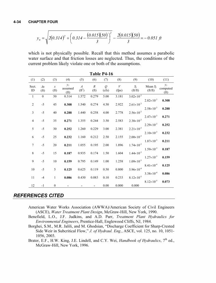
where xc is measured from the upstream end of the channel. Then q = (0.1 × 57.85)/5 = 1.156 cfs/ft and yc = 0.346 ft. This new critical depth is used with Equation 4-35 to compute a new value of xc. The iterative process continues until the assumed and computed critical depths sufficiently match. For the current problem, convergence occurs at xc = 57.15 ft, q = 1.143 cfs/ft, and yc = 0.344 ft. Since xc exceeds the length of the channel, critical flow occurs at the downstream end of the channel and flow in the channel is subcritical. The corresponding water surface profile is evaluated using Equation 4-34; computations begin at the critical section and proceed upstream. Table P4-16 summarizes the analysis and is self explanatory in nature. For each incremental channel reach, the objective is to obtain a match between the assumed upstream depth and the depth computed via Equation 4-34. Note that at the far upstream end, where x = 0, Q, V, and Sf are zero, application of Equation 4-34 reduces to
( )( )g
VxxSSyy2
121fo21 +−−=−
where subscript 1 refers to conditions at section 11. As shown, the analysis yields an upstream depth of 0.073 ft.
Problem 4.17 Collection channel For the conditions described in Problem 4.16, estimate the depth at the upstream end of the channel by using the approximation represented by Equation 4-37.
Solution
From Problem 4.16, the critical depth is 0.314 ft. Thus,
4-34 CHAPTER FOUR
( ) ( )( ) ( )( ) ft 051.0 3
50015.023
50015.0314.0314.02y2
2u −=−⎟
⎠⎞
⎜⎝⎛ −+=
which is not physically possible. Recall that this method assumes a parabolic water surface and that friction losses are neglected. Thus, the conditions of the current problem likely violate one or both of the assumptions.
American Water Works Association (AWWA)/American Society of Civil Engineers (ASCE), Water Treatment Plant Design, McGraw-Hill, New York, 1990.
Benefield, L.O., J.F. Judkins, and A.D. Parr, Treatment Plant Hydraulics for Environmental Engineers, Prentice-Hall, Englewood Cliffs, NJ, 1984.
Borghei, S.M., M.R. Jalili, and M. Ghodsian, “Discharge Coefficient for Sharp-Crested Side Weir in Subcritical Flow,” J. of Hydraul. Eng., ASCE, vol. 125, no. 10, 1051-1056, 2003.
Brater, E.F., H.W. King, J.E. Lindell, and C.Y. Wei, Handbook of Hydraulics, 7th ed., McGraw-Hill, New York, 1996.
FLOW MEASUREMENT AND CONTROL 4-35
Chadwick, A.J., and J.C. Morfett, Hydraulics in Civil Engineering, Allen and Unwin, London, 1986.
Chaudhry, M.H., Open-Channel Flow, Prentice-Hall, Englewood Cliffs, NJ, 1993. Chow, V.T., Open Channel Hydraulics, McGraw-Hill, New York, 1959. De Marchi, G., “Essay on the Performance of Lateral Weirs,” L’Energia Eletrica, vol.
11, no. 11, 1934. El-Khashab, A., and K.V.H. Smith, “Experimental Investigation of Flow Over Side
Weirs,” J. of Hydraul. Eng., ASCE, vol. 102, no. 9, 1255-1268, 1976. Ghodsian, M., “Flow Through Side Sluice Gate,” J. of Irrig. and Drainage Engrg.,
ASCE, vol. 129, no. 6, 458-463, 2003. Gisonni, C., and W.H. Hager, “Short Sewer Sideweir,” J. of Irrig. and Drainage
Engrg., ASCE, vol. 123, no. 5, 354-363, 1995. Hager, W.H., “Lateral Outflow Over Side Weirs,” J. of Hydraul. Eng., ASCE, vol. 113,
no. 4, 491-504, 1987. Henderson, F.M., Open Channel Flow, Macmillan, New York, 1966. Maisch, F.E., T.J. Sullivan, R.J. Cronin, F.J. Tantone, D.V. Hobbs, W.L. Judy, and S.L.
Cole, “Water and Wastewater Treatment Plant Hydraulics,” in Hydraulic Design Handbook, ed. by L.W. Mays, McGraw Hill, New York, 1999.
Metcalf and Eddy, Inc., Wastewater Engineering: Treatment, Disposal, and Reuse, 3rd ed., McGraw-Hill, New York, 1991.
Muslu, Y., “Numerical Analysis for Lateral Weir Flow,” J. of Irrig. and Drainage Eng., ASCE, vol. 127, no. 4, 246-253, 2001.
Parshall, R.L., “Measuring Water in Irrigation Channels with Parshall Flumes and Small Weirs,” U.S. Soil Conservation Service, Circular 843, U.S. Dept. of Agriculture, Washington, DC, 1950.
Potter, M.C., and D.C. Wiggert, Mechanics of Fluids, 2nd ed., Brooks/Cole, Pacific Grove, CA, 2002.
Rawn, A.M., F.R. Bowerman, and N.H. Brooks, “Diffusers for Disposal of Sewage in Sea Water,” Trans. ASCE, 126, Part III, 344-388, 1961.