4F5: Advanced Wireless Communications Handout 7: Characterisation of Fading Channels Jossy Sayir and Tobias Koch Signal Processing and Communications Lab Department of Engineering University of Cambridge {jossy.sayir,tobi.koch}@eng.cam.ac.uk Lent 2012 c J. Sayir and T. Koch (CUED) Advanced Wireless Communications Lent 2012 1 / 12
Transcript
4F5: Advanced Wireless CommunicationsHandout 7: Characterisation of Fading Channels
Jossy Sayir and Tobias Koch
Signal Processing and Communications LabDepartment of Engineering
University of Cambridge{jossy.sayir,tobi.koch}@eng.cam.ac.uk
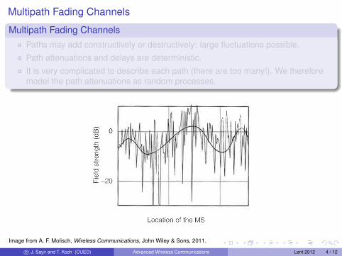
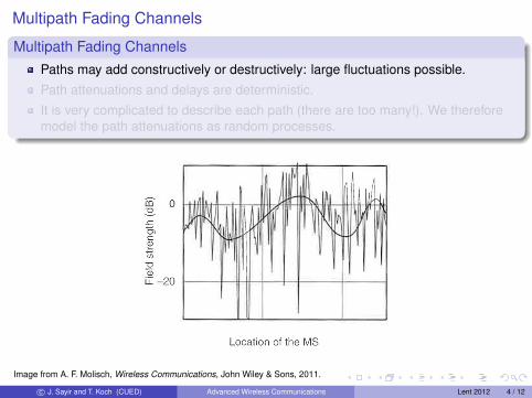
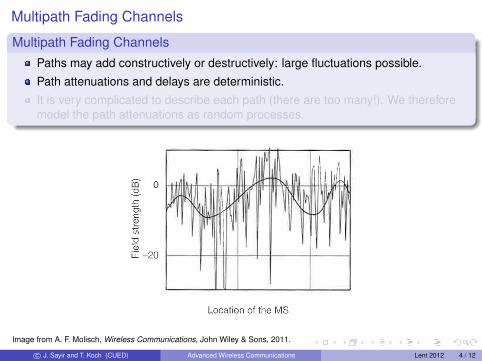
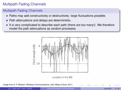
Multipath Fading ChannelsChannel Correlation Functions and Power Spectra
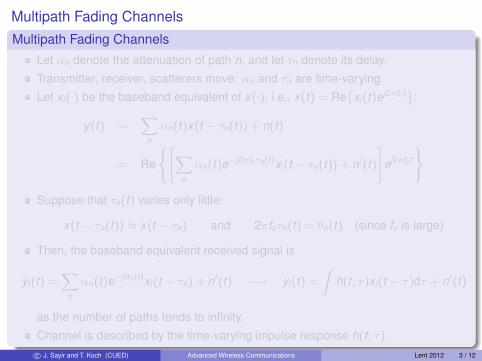
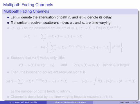
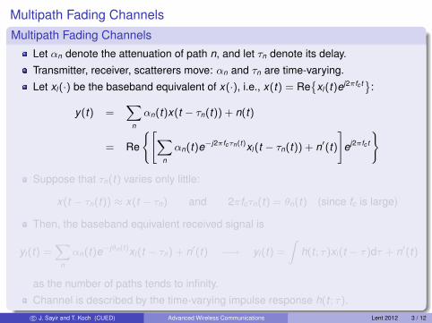
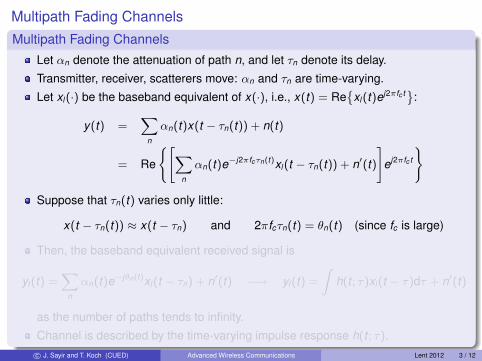
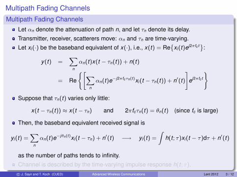
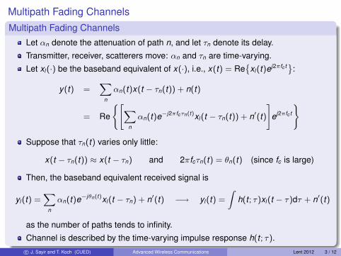
Time-varying impulse response h(t ; τ) is modelled as complex random process.
Let Rh(t1, t2; τ1, τ2) , E[h(t1; τ1)∗h(t2; τ2)]. The WSSUS assumption is:I {h(t ; τ), t ∈ R} is wide sense stationary, i.e., E[h(t ; τ)] does not depend on t ,
Rh(t1, t2; τ1, τ2) = Rh(t1 − t2, 0; τ1, τ2) and Rh(0, 0; τ1, τ2) <∞I Scatterers are uncorrelated, so
Rh(t1, t2; τ1, τ2) = Rh(t1, t2; τ1, τ1)δ(τ2 − τ1)
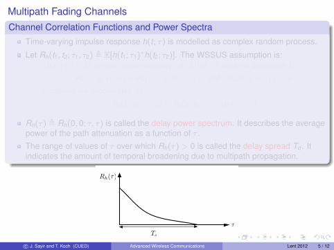
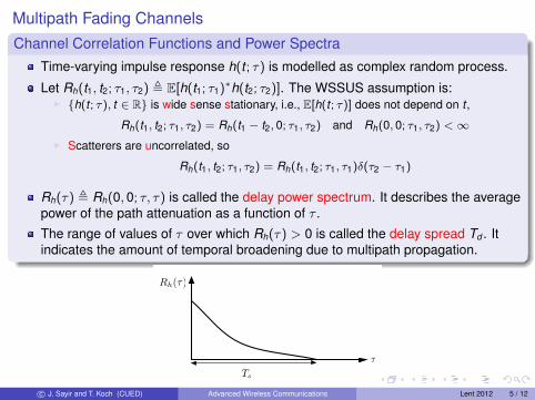
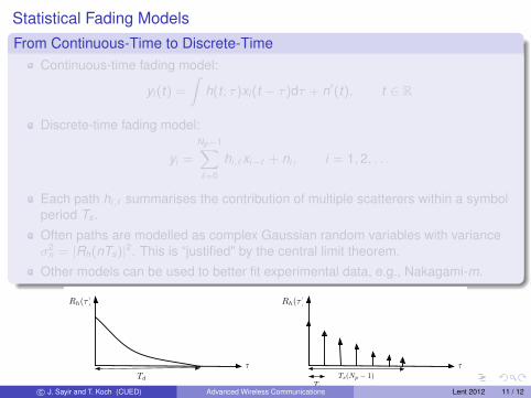
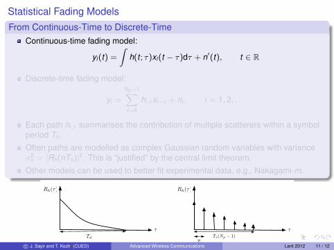
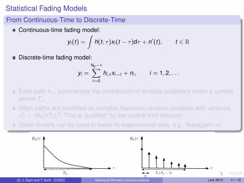
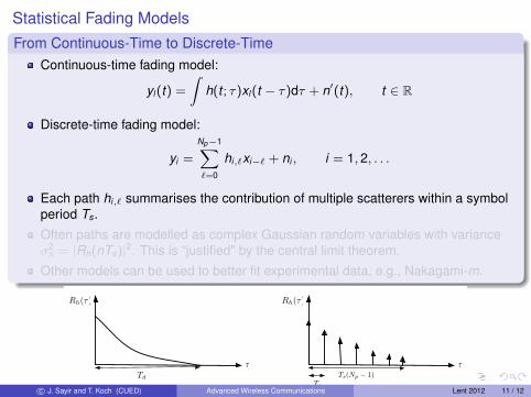
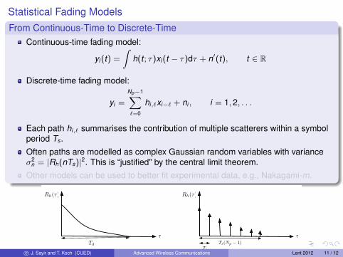
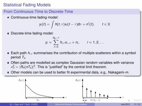
Rh(τ) , Rh(0, 0; τ, τ) is called the delay power spectrum. It describes the averagepower of the path attenuation as a function of τ .
The range of values of τ over which Rh(τ) > 0 is called the delay spread Td . Itindicates the amount of temporal broadening due to multipath propagation.
Multipath Fading ChannelsChannel Correlation Functions and Power Spectra
Time-varying impulse response h(t ; τ) is modelled as complex random process.
Let Rh(t1, t2; τ1, τ2) , E[h(t1; τ1)∗h(t2; τ2)]. The WSSUS assumption is:I {h(t ; τ), t ∈ R} is wide sense stationary, i.e., E[h(t ; τ)] does not depend on t ,
Rh(t1, t2; τ1, τ2) = Rh(t1 − t2, 0; τ1, τ2) and Rh(0, 0; τ1, τ2) <∞I Scatterers are uncorrelated, so
Rh(t1, t2; τ1, τ2) = Rh(t1, t2; τ1, τ1)δ(τ2 − τ1)
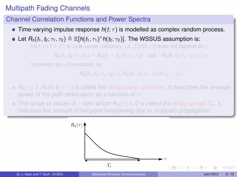
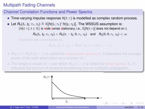
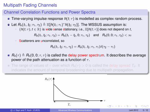
Rh(τ) , Rh(0, 0; τ, τ) is called the delay power spectrum. It describes the averagepower of the path attenuation as a function of τ .
The range of values of τ over which Rh(τ) > 0 is called the delay spread Td . Itindicates the amount of temporal broadening due to multipath propagation.
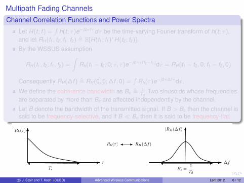
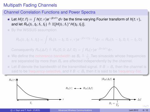
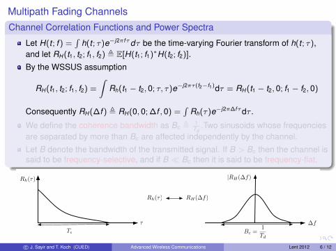
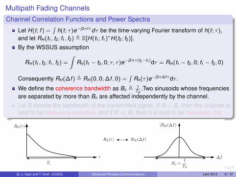
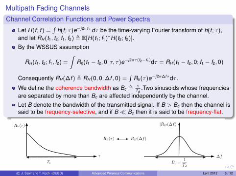
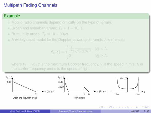
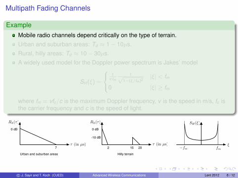
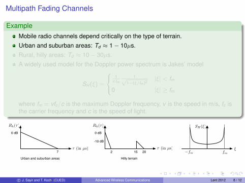
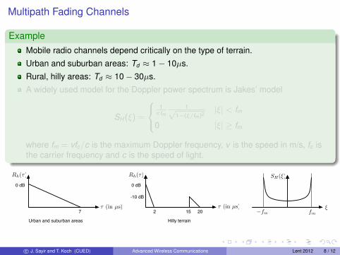
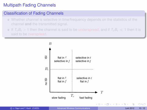
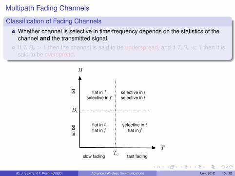
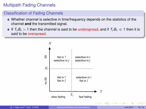
.Two sinusoids whose frequenciesare separated by more than Bc are affected independently by the channel.
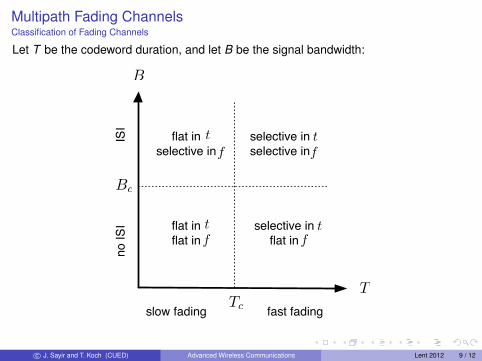
Let B denote the bandwidth of the transmitted signal. If B > Bc then the channel issaid to be frequency-selective, and if B � Bc then it is said to be frequency-flat.
.Two sinusoids whose frequenciesare separated by more than Bc are affected independently by the channel.
Let B denote the bandwidth of the transmitted signal. If B > Bc then the channel issaid to be frequency-selective, and if B � Bc then it is said to be frequency-flat.
.Two sinusoids whose frequenciesare separated by more than Bc are affected independently by the channel.
Let B denote the bandwidth of the transmitted signal. If B > Bc then the channel issaid to be frequency-selective, and if B � Bc then it is said to be frequency-flat.
.Two sinusoids whose frequenciesare separated by more than Bc are affected independently by the channel.
Let B denote the bandwidth of the transmitted signal. If B > Bc then the channel issaid to be frequency-selective, and if B � Bc then it is said to be frequency-flat.
.Two sinusoids whose frequenciesare separated by more than Bc are affected independently by the channel.
Let B denote the bandwidth of the transmitted signal. If B > Bc then the channel issaid to be frequency-selective, and if B � Bc then it is said to be frequency-flat.
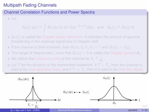
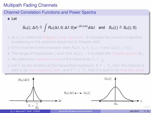
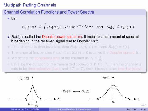
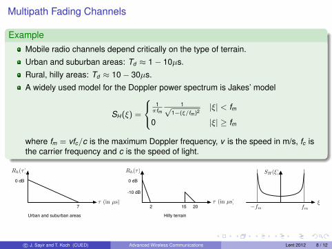
SH(ξ) is called the Doppler power spectrum. It indicates the amount of spectralbroadening in the received signal due to Doppler shift.
If the channel is time-invariant, then RH(t1, t2; f1, f1) = 1 and SH(ξ) = δ(ξ).
The range of frequencies ξ such that SH(ξ) > 0 is called the Doppler spread Bd .
We define the coherence time of the channel as Tc , 1Bd
.
Let T be the duration of the transmitted codeword. If T > Tc , then the channel issaid to be time-selective (fast), and if T � Tc , then it is said to be time-flat (slow).
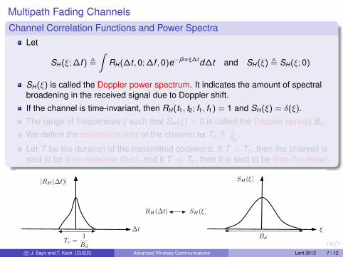
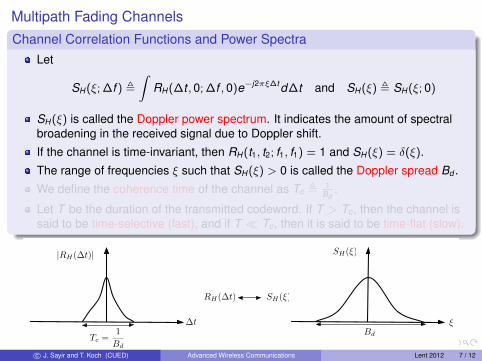
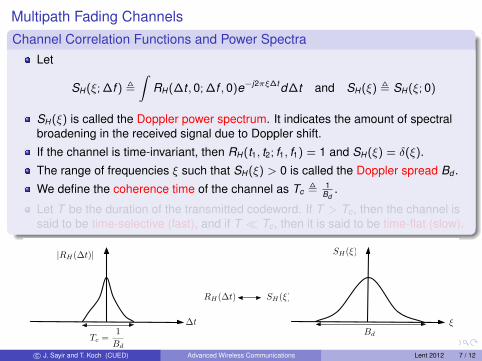


![Mendel’s Manuscript of ‘Versuche über Pflanzenhybriden ...UH/Simu... · Größe“ [Our Contribution to the Common Greatness] and Molisch, H. (1934) Erinnerungen und Welteindrücke](https://static.documents.pub/doc/80x56/5e099f451ca39074d4783d62/mendelas-manuscript-of-aversuche-ber-pflanzenhybriden-uhsimu-greaoe.jpg)


