56
03/17/22 Tactical Asset Allocation 1 Tactical Asset Allocation Tactical Asset Allocation 2 2 session session 6 6 Andrei Simonov
| Date post: | 18-Dec-2015 |
| Category: |
Documents |
| Upload: | barnaby-russell |
| View: | 225 times |
| Download: | 0 times |
04/18/23Tactical Asset Allocation1
Tactical Asset Allocation 2Tactical Asset Allocation 2sessionsession 6 6
Andrei Simonov
04/18/23Tactical Asset Allocation2
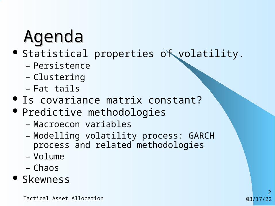
AgendaAgenda Statistical properties of volatility.
– Persistence– Clustering– Fat tails
Is covariance matrix constant? Predictive methodologies
– Macroecon variables– Modelling volatility process: GARCH process and related
methodologies– Volume– Chaos
Skewness
04/18/23Tactical Asset Allocation3
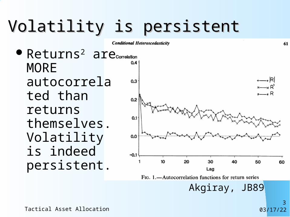
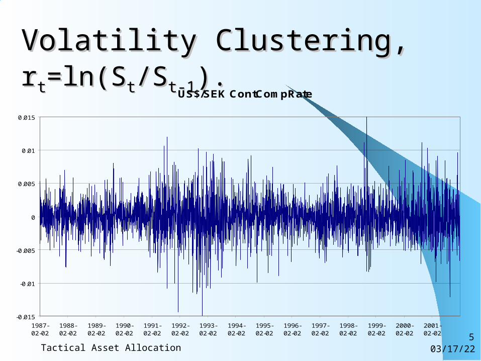
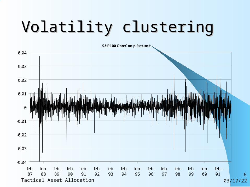
Volatility is persistentVolatility is persistent
Returns2 are MORE autocorrelated than returns themselves. Volatility is indeed persistent.
Akgiray, JB89
04/18/23Tactical Asset Allocation4
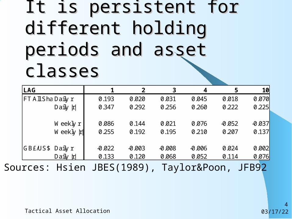
It is persistent for different It is persistent for different holding periods and asset holding periods and asset classesclasses
LAG 1 2 3 4 5 10FT All Share Daily r 0.193 0.020 0.031 0.045 0.018 0.070
Daily |r| 0.347 0.292 0.256 0.260 0.222 0.225
Weekly r 0.086 0.144 0.021 0.076 -0.052 -0.037Weekly |r| 0.255 0.192 0.195 0.210 0.207 0.137
GB£/US$ Daily r -0.022 -0.003 -0.008 -0.006 0.024 0.002Daily |r| 0.133 0.120 0.068 0.052 0.114 0.076
Sources: Hsien JBES(1989), Taylor&Poon, JFB92
04/18/23Tactical Asset Allocation5
Volatility Clustering, Volatility Clustering, rrtt=ln(S=ln(Stt/S/St-1t-1).). US$/SEK ContCompRate
-0.015
-0.01
-0.005
0
0.005
0.01
0.015
1987-02-02
1988-02-02
1989-02-02
1990-02-02
1991-02-02
1992-02-02
1993-02-02
1994-02-02
1995-02-02
1996-02-02
1997-02-02
1998-02-02
1999-02-02
2000-02-02
2001-02-02
04/18/23Tactical Asset Allocation6
Volatility clusteringVolatility clusteringS&P100 ContComp Returns
-0.04
-0.03
-0.02
-0.01
0
0.01
0.02
0.03
0.04
feb-87
feb-88
feb-89
feb-90
feb-91
feb-92
feb-93
feb-94
feb-95
feb-96
feb-97
feb-98
feb-99
feb-00
feb-01
04/18/23Tactical Asset Allocation7
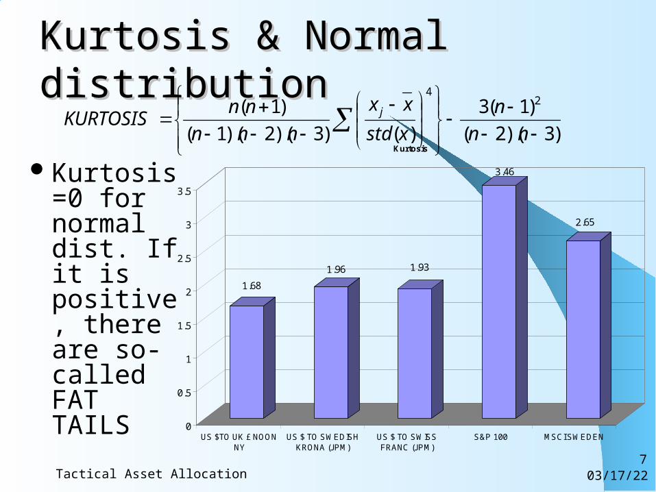
Kurtosis & Normal distributionKurtosis & Normal distribution
Kurtosis=0 for normal dist. If it is positive, there are so-called FAT TAILS
)3)(2(
)1(3
)()3)(2)(1(
)1( 24
nn
n
xstd
xx
nnn
nnKURTOSIS j
1.68
1.96 1.93
3.46
2.65
0
0.5
1
1.5
2
2.5
3
3.5
US $TO UK £ NOONNY
US $ TO SWEDISHKRONA (JPM)
US $ TO SWISSFRANC (JPM)
S&P 100 MSCI SWEDEN
Kurtosis
04/18/23Tactical Asset Allocation8
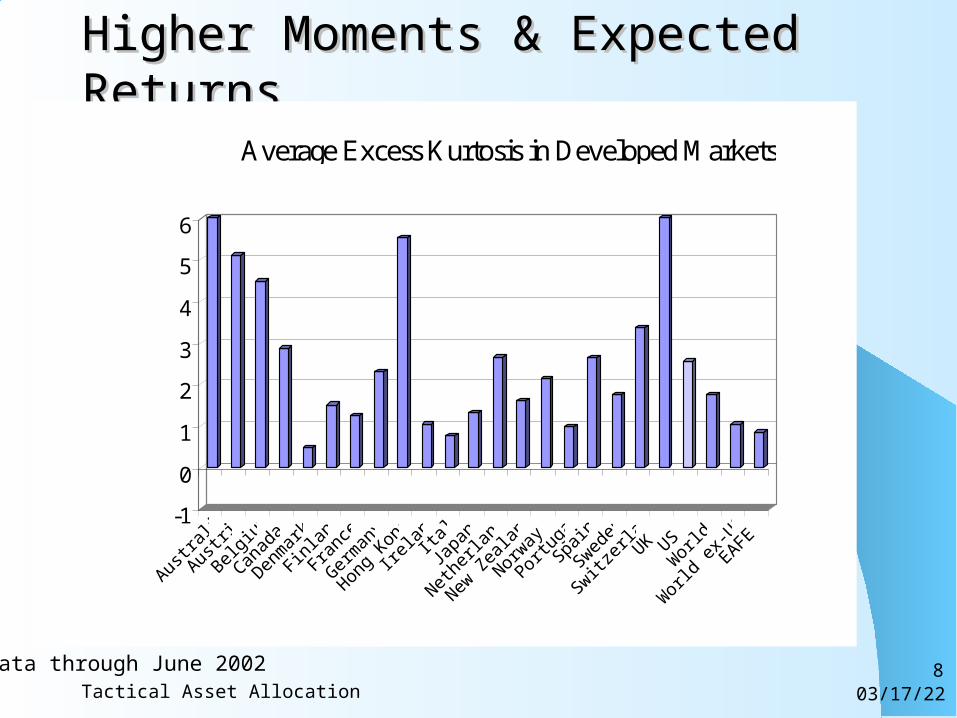
Higher Moments & Expected ReturnsHigher Moments & Expected Returns
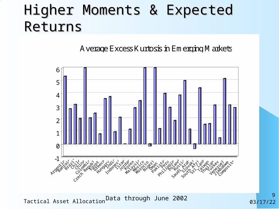
Data through June 2002
-1
0
1
2
3
4
5
6
Australi
a
Austria
Belg
ium
Canad
a
Den
mar
k
Finlan
d
France
Ger
man
y
Hong K
ong
Irelan
d It
aly
Japan
Nether
lands
New
Zea
land
Norway
Portugal
Spain
Swed
en
Switzer
land UK US
World
World
ex-U
S
EAFE
Average Excess Kurtosis in Developed Markets
04/18/23Tactical Asset Allocation9
Higher Moments & Expected ReturnsHigher Moments & Expected Returns
Data through June 2002
-1
0
1
2
3
4
5
6
Argen
tina
Bahrai
n
Brazil
Chile
China
Colombia
Czech
Rep
ublicEgy
pt
Greece
Hunga
ry
India
Indo
nesia
Israe
l
Jord
an
Korea
Mala
ysia
Mex
ico
Mor
occo
Nigeria
Oman
Pakist
an
Peru
Philipp
ines
Poland
Russia
Saudi
Arabia
Slovak
ia
South
Africa
Sri Lan
ka
Taiw
an
Thaila
nd
Turke
y
Venez
uela
Zimba
bwe
Compo
site
Average Excess Kurtosis in Emerging Markets
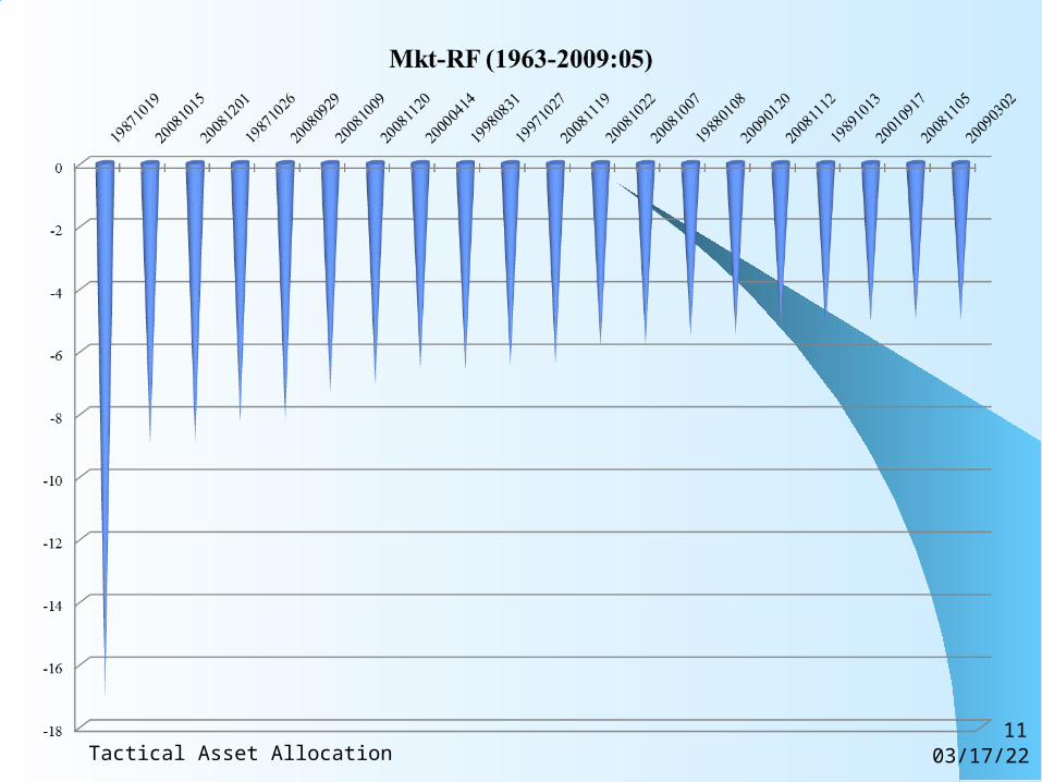
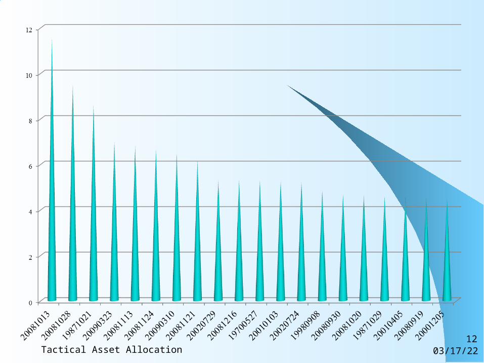
04/18/23Tactical Asset Allocation10
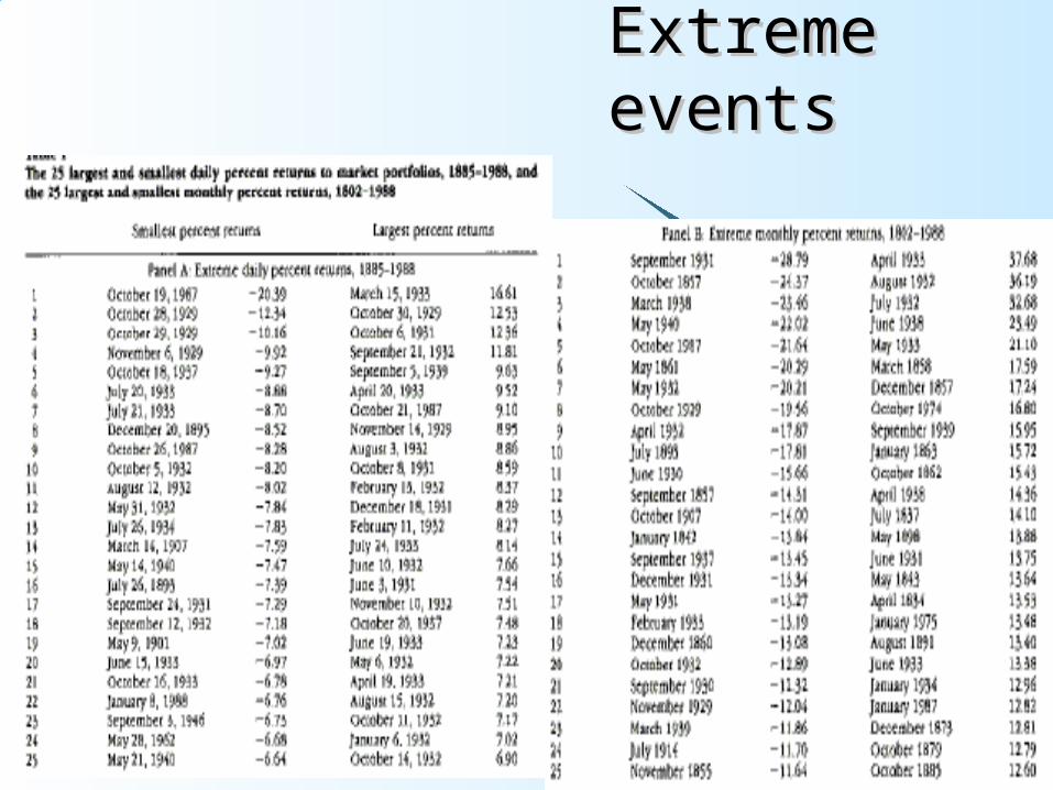
Extreme Extreme eventsevents
04/18/23Tactical Asset Allocation11
04/18/23Tactical Asset Allocation12
04/18/23Tactical Asset Allocation13
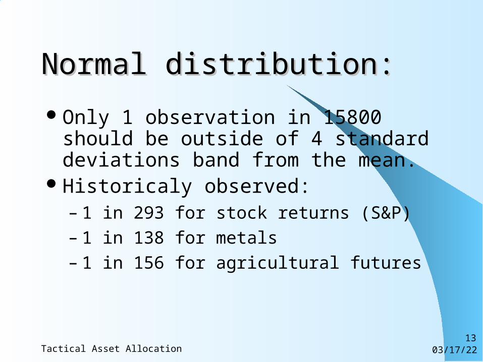
Normal distribution:Normal distribution:
Only 1 observation in 15800 should be outside of 4 standard deviations band from the mean.
Historicaly observed:– 1 in 293 for stock returns (S&P)– 1 in 138 for metals– 1 in 156 for agricultural futures
04/18/23Tactical Asset Allocation14
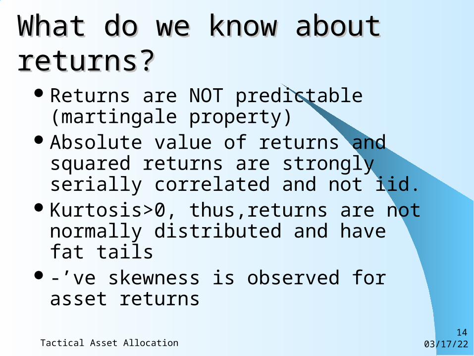
What do we know about returns?What do we know about returns?
Returns are NOT predictable (martingale property)
Absolute value of returns and squared returns are strongly serially correlated and not iid.
Kurtosis>0, thus,returns are not normally distributed and have fat tails
-’ve skewness is observed for asset returns
04/18/23Tactical Asset Allocation15
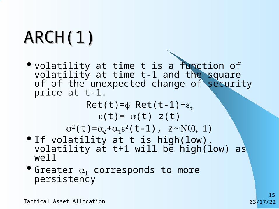
ARCH(1)ARCH(1)
volatility at time t is a function of volatility at time t-1 and the square of of the unexpected change of security price at t-1.
Ret(t)= Ret(t-1)+t
(t)= (t) z(t)2(t)=0+12(t-1), z)
If volatility at t is high(low), volatility at t+1 will be high(low) as well
Greater 1 corresponds to more persistency
04/18/23Tactical Asset Allocation16
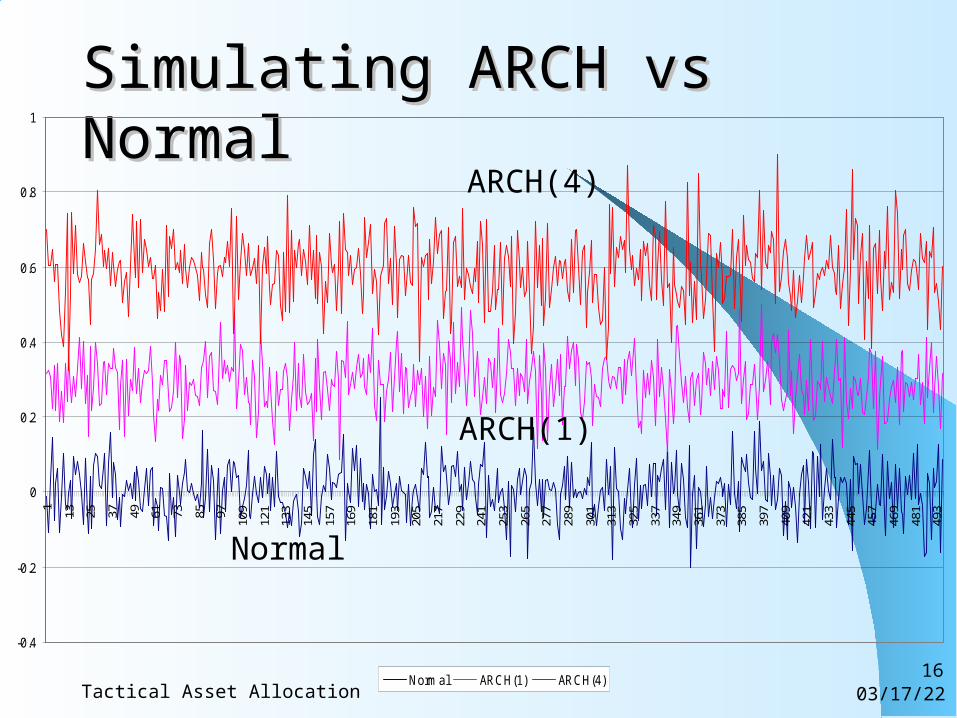
Simulating ARCH vs NormalSimulating ARCH vs Normal
-0.4
-0.2
0
0.2
0.4
0.6
0.8
1
1
13 25 37 49 61 73 85 97
109
121
133
145
157
169
181
193
205
217
229
241
253
265
277
289
301
313
325
337
349
361
373
385
397
409
421
433
445
457
469
481
493
Normal ARCH(1) ARCH(4)
Normal
ARCH(1)
ARCH(4)
04/18/23Tactical Asset Allocation17
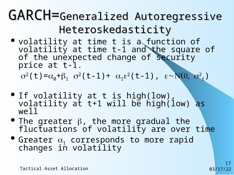
GARCH=GARCH=Generalized Autoregressive Generalized Autoregressive HeteroskedasticityHeteroskedasticity
volatility at time t is a function of volatility at time t-1 and the square of of the unexpected change of security price at t-1.
2(t)=0+1 2(t-1)+ 12(t-1), 2t)
If volatility at t is high(low), volatility at t+1 will be high(low) as well
The greater , the more gradual the fluctuations of volatility are over time
Greater 1 corresponds to more rapid changes in volatility
04/18/23Tactical Asset Allocation18
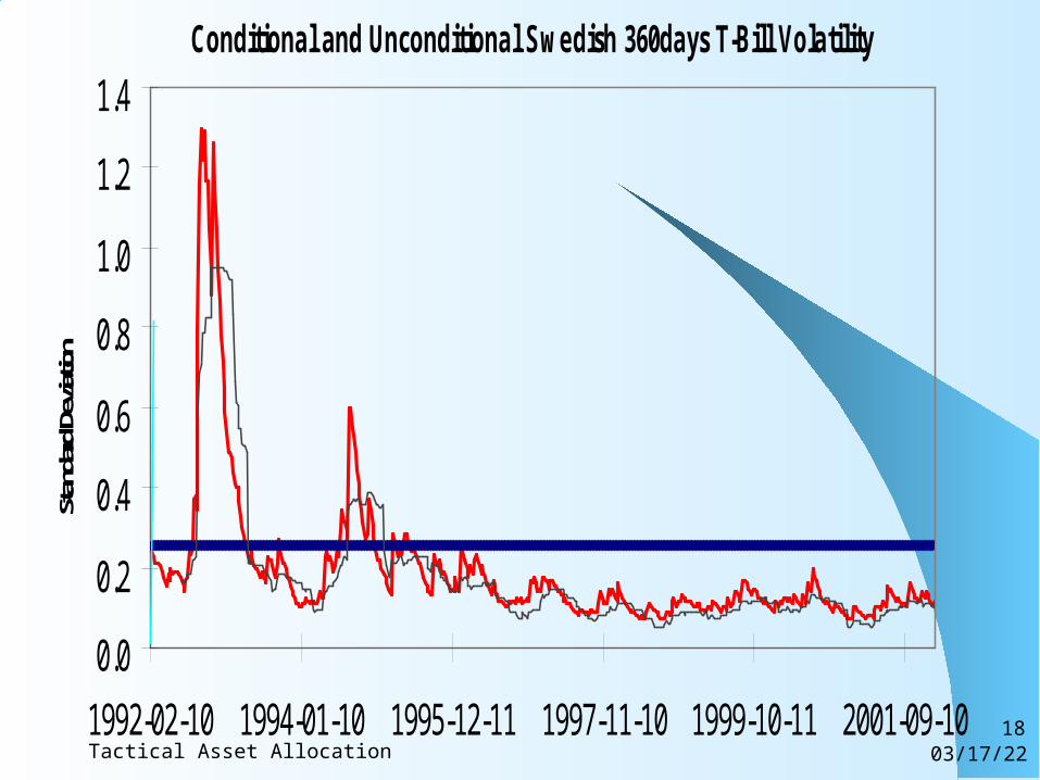
Conditional and Unconditional Swedish 360days T-Bill Volatility
0.0
0.2
0.4
0.6
0.8
1.0
1.2
1.4
1992-02-10 1994-01-10 1995-12-11 1997-11-10 1999-10-11 2001-09-10
Stan
dard
Dev
iation
04/18/23Tactical Asset Allocation19
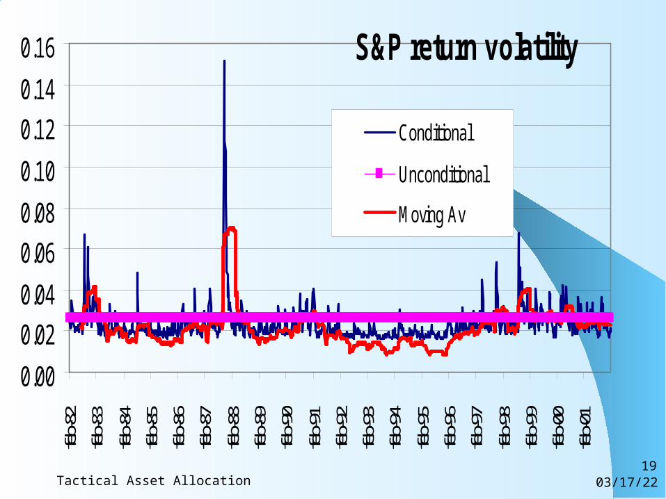
S&P return volatility
0.00
0.02
0.04
0.06
0.08
0.10
0.12
0.14
0.16feb
-82feb
-83feb
-84feb
-85feb
-86feb
-87feb
-88feb
-89feb
-90feb
-91feb
-92feb
-93feb
-94feb
-95feb
-96feb
-97feb
-98feb
-99feb
-00feb
-01
Conditional
Unconditional
Moving Av
04/18/23Tactical Asset Allocation20
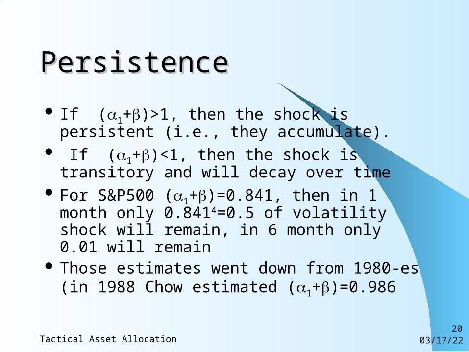
PersistencePersistence
If (1+)>1, then the shock is persistent (i.e., they accumulate).
If (1+)<1, then the shock is transitory and will decay over time
For S&P500 (1+)=0.841, then in 1 month only 0.8414=0.5 of volatility shock will remain, in 6 month only 0.01 will remain
Those estimates went down from 1980-es (in 1988 Chow estimated (1+)=0.986
04/18/23Tactical Asset Allocation21
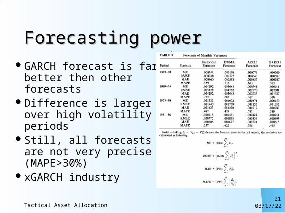
Forecasting powerForecasting power
GARCH forecast is far better then other forecasts
Difference is larger over high volatility periods
Still, all forecasts are not very precise (MAPE>30%)
xGARCH industry
04/18/23Tactical Asset Allocation22
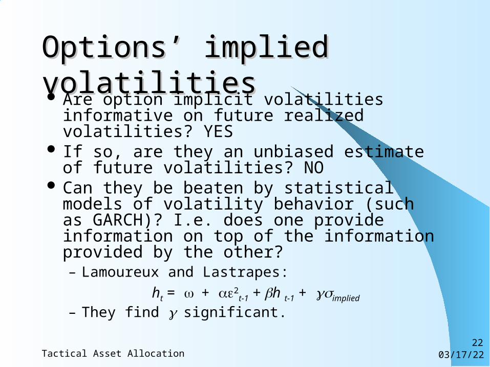
Options’ implied volatilitiesOptions’ implied volatilities Are option implicit volatilities informative on
future realized volatilities? YES If so, are they an unbiased estimate of future
volatilities? NO Can they be beaten by statistical models of
volatility behavior (such as GARCH)? I.e. does one provide information on top of the information provided by the other?– Lamoureux and Lastrapes:
ht = + 2t-1 + h t-1 + implied
– They find significant.
04/18/23Tactical Asset Allocation23
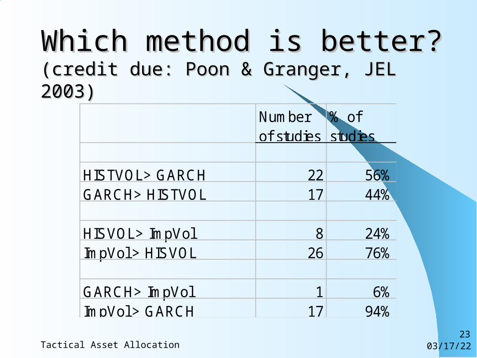
Which method is better?Which method is better?(credit due: Poon & Granger, JEL 2003)(credit due: Poon & Granger, JEL 2003)
Number of studies
% of studies
HISTVOL> GARCH 22 56%GARCH> HISTVOL 17 44%
HISVOL> ImpVol 8 24%ImpVol > HISVOL 26 76%
GARCH> ImpVol 1 6%ImpVol > GARCH 17 94%
04/18/23Tactical Asset Allocation24
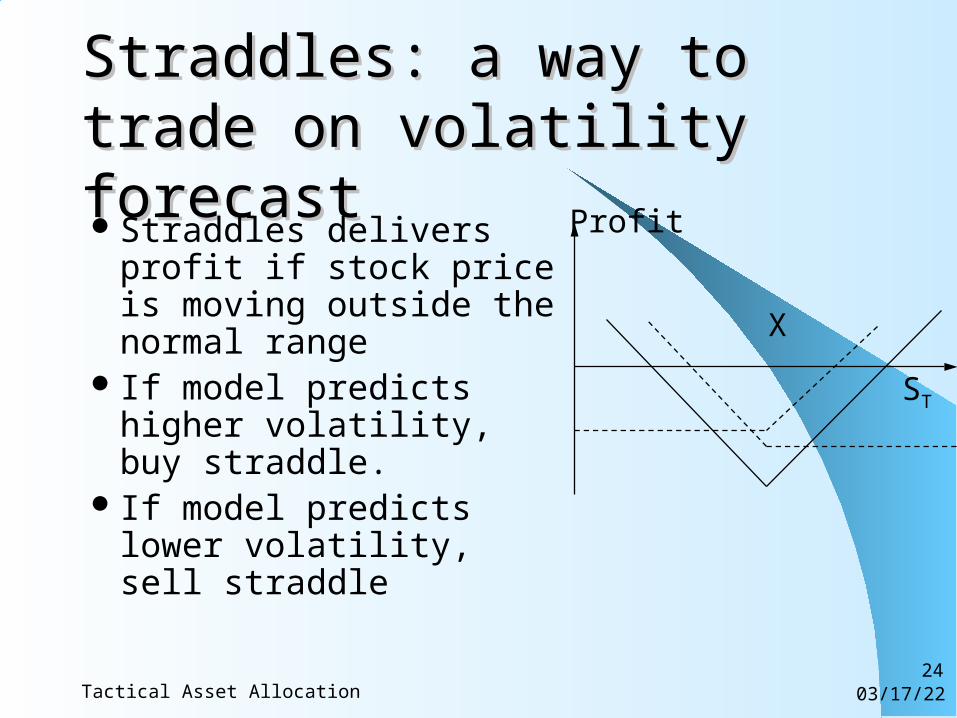
Straddles: a way to trade on Straddles: a way to trade on volatility forecastvolatility forecastStraddles delivers profit
if stock price is moving outside the normal range
If model predicts higher volatility, buy straddle.
If model predicts lower volatility, sell straddle
ST
X
Profit
04/18/23Tactical Asset Allocation25
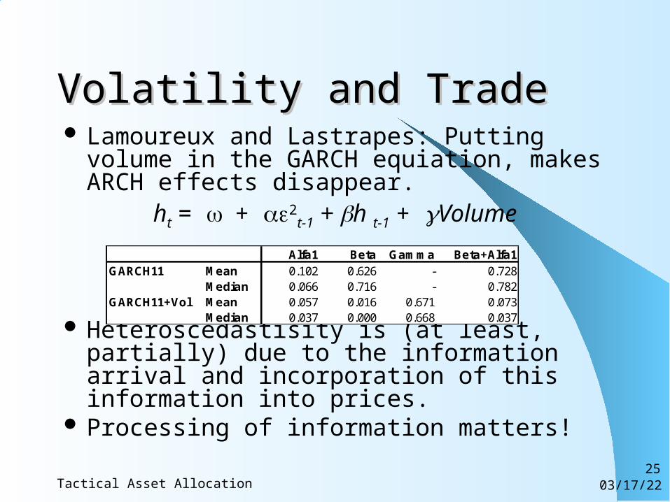
Volatility and Trade Volatility and Trade Lamoureux and Lastrapes: Putting volume in the
GARCH equiation, makes ARCH effects disappear.
ht = + 2t-1 + h t-1 + Volume
Heteroscedastisity is (at least, partially) due to the information arrival and incorporation of this information into prices.
Processing of information matters!
Alfa1 Beta Gamma Beta+Alfa1GARCH11 Mean 0.102 0.626 - 0.728
Median 0.066 0.716 - 0.782GARCH11+Vol Mean 0.057 0.016 0.671 0.073
Median 0.037 0.000 0.668 0.037
04/18/23Tactical Asset Allocation26
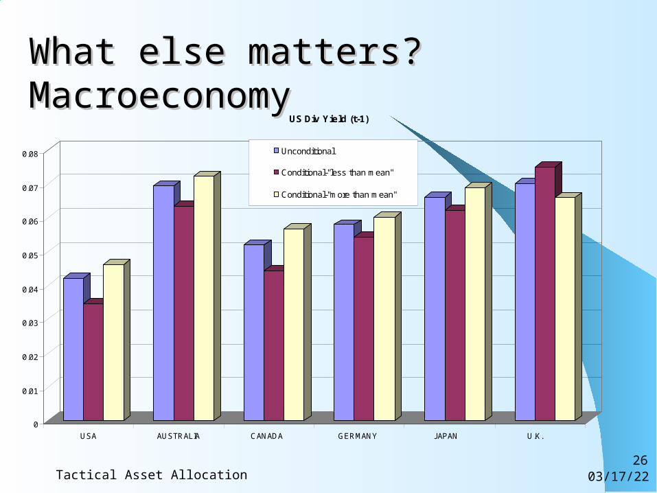
What else matters? MacroeconomyWhat else matters? Macroeconomy
0
0.01
0.02
0.03
0.04
0.05
0.06
0.07
0.08
USA AUSTRALIA CANADA GERMANY JAPAN U.K.
US Div Yield (t-1)
Unconditional
Conditional-"less than mean"
Conditional-"more than mean"
04/18/23Tactical Asset Allocation27
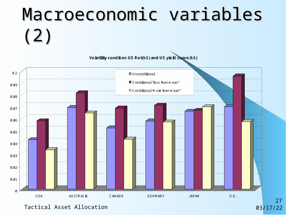
Macroeconomic variables (2)Macroeconomic variables (2)
0
0.01
0.02
0.03
0.04
0.05
0.06
0.07
0.08
0.09
0.1
USA AUSTRALIA CANADA GERMANY JAPAN U.K.
Volatility condit on US Ret(t-1) and US yield curve(t-1)
Unconditional
Conditional-"less than mean"
Conditional-"more than mean"
04/18/23Tactical Asset Allocation28
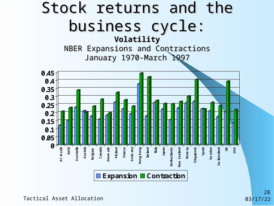
Stock returns and the business cycle:Stock returns and the business cycle:VolatilityVolatility
NBER Expansions and ContractionsNBER Expansions and ContractionsJanuary 1970-March 1997January 1970-March 1997
00.050.1
0.150.2
0.250.3
0.350.4
0.45
AC
Wo
rld
EAFE
Au
str
alia
Au
str
ia
Be
lgiu
m
Can
ada
De
nm
ark
Fin
lan
d
Fran
ce
Ge
rman
y
Ho
ng
Ko
ng
Ire
lan
d
Ital
y
Jap
an
Ne
the
rlan
ds
Ne
w Z
eal
and
No
rway
Sin
gap
ore
Sp
ain
Sw
ed
en
Sw
itze
rlan
d
UK
US
A
Expansion Contraction
04/18/23Tactical Asset Allocation29
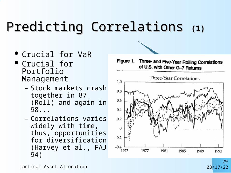
Predicting Correlations Predicting Correlations (1)(1)
Crucial for VaR Crucial for Portfolio
Management– Stock markets crash
together in 87 (Roll) and again in 98...
– Correlations varies widely with time, thus, opportunities for diversification (Harvey et al., FAJ 94)
04/18/23Tactical Asset Allocation30
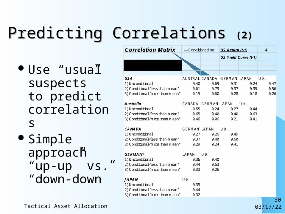
Predicting Correlations Predicting Correlations (2)(2)
Use “usual suspects” to predict correlations
Simple approach “up-up” vs. “down-down”
Correlation Matrix --- Conditioned on: US Return (t-1) &
US Yield Curve (t-1)
Remove Black Monday ?yes
USA AUSTRALIACANADA GERMANY JAPAN U.K. 1) Unconditional 0.40 0.69 0.31 0.24 0.472) Conditional-"less than mean" 0.61 0.79 0.37 0.35 0.563) Conditional-"more than mean" 0.19 0.60 0.28 0.18 0.26
Australia CANADA GERMANY JAPAN U.K. 1) Unconditional 0.55 0.24 0.27 0.442) Conditional-"less than mean" 0.65 0.40 0.40 0.633) Conditional-"more than mean" 0.46 0.06 0.21 0.41
CANADA GERMANY JAPAN U.K. 1) Unconditional 0.27 0.26 0.492) Conditional-"less than mean" 0.37 0.40 0.603) Conditional-"more than mean" 0.29 0.24 0.41
GERMANY JAPAN U.K. 1) Unconditional 0.36 0.402) Conditional-"less than mean" 0.44 0.533) Conditional-"more than mean" 0.33 0.26
JAPAN U.K. 1) Unconditional 0.352) Conditional-"less than mean" 0.443) Conditional-"more than mean" 0.32
04/18/23Tactical Asset Allocation31
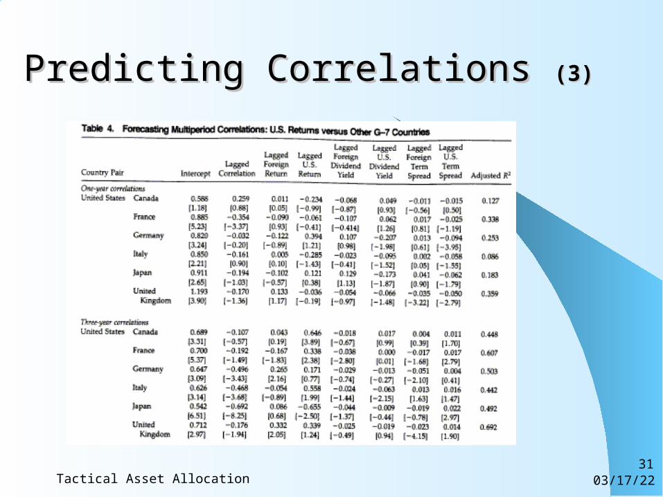
Predicting Correlations Predicting Correlations (3)(3)
04/18/23Tactical Asset Allocation32
Chaos as alternative to Chaos as alternative to stochastic modelingstochastic modeling
Chaos in deterministic non-linear dynamic system that can produce random-looking results
Feedback systems, x(t)=f(x(t-1), x(t-2)...) Critical levels: if x(t) exceeds x0, the system can start
behaving differently (line 1929, 1987, 1989, etc.) The attractiveness of chaotic dynamics is in its ability
to generate large movements which appear to be random with greater frequency than linear models (Noah effect)
Long memory of the process (Joseph effect)
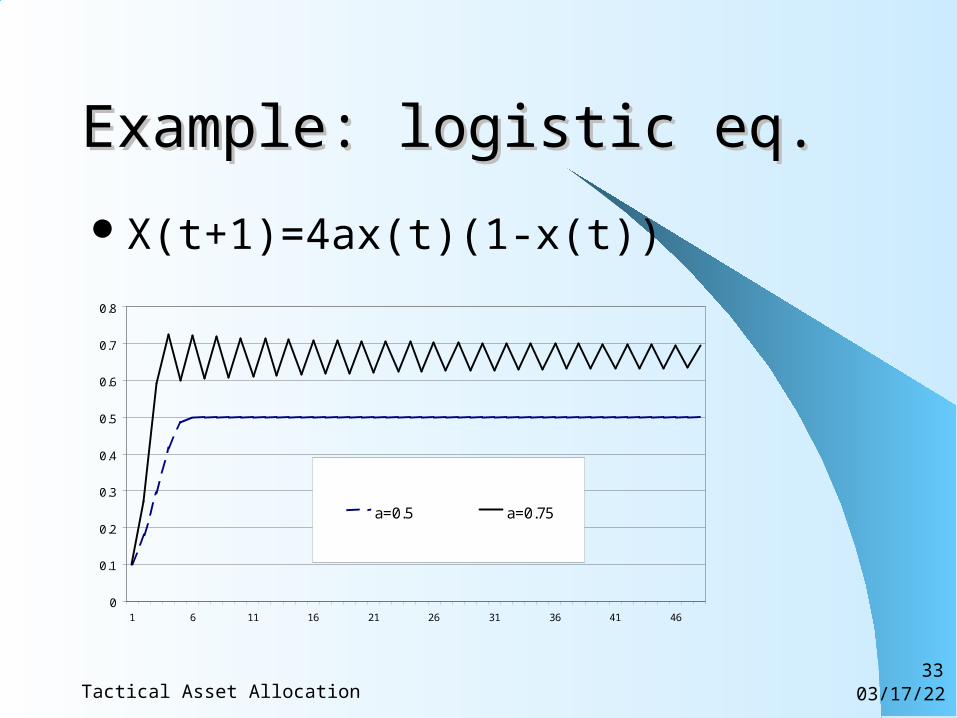
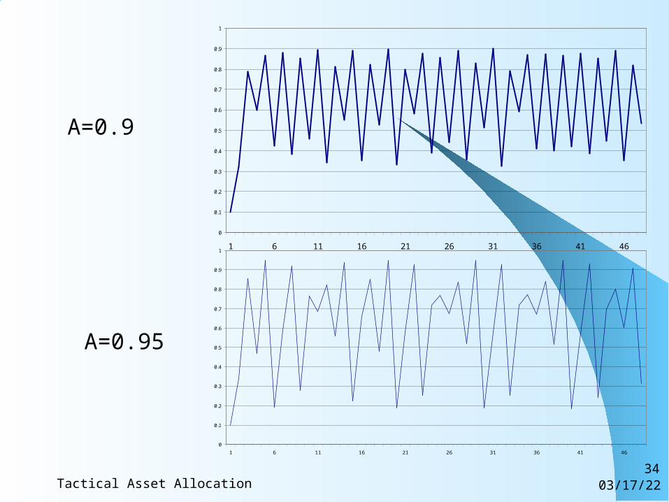
04/18/23Tactical Asset Allocation33
Example: logistic eq.Example: logistic eq.
X(t+1)=4ax(t)(1-x(t))
0
0.1
0.2
0.3
0.4
0.5
0.6
0.7
0.8
1 6 11 16 21 26 31 36 41 46
a=0.5 a=0.75
04/18/23Tactical Asset Allocation34
0
0.1
0.2
0.3
0.4
0.5
0.6
0.7
0.8
0.9
1
1 6 11 16 21 26 31 36 41 46
0
0.1
0.2
0.3
0.4
0.5
0.6
0.7
0.8
0.9
1
1 6 11 16 21 26 31 36 41 46
A=0.9
A=0.95
04/18/23Tactical Asset Allocation35
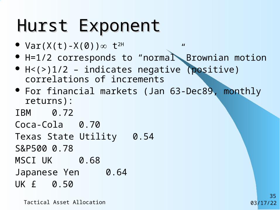
Hurst ExponentHurst Exponent Var(X(t)-X(0)) t2H
H=1/2 corresponds to “normal” Brownian motion H<(>)1/2 – indicates negative (positive) correlations of
increments For financial markets (Jan 63-Dec89, monthly returns):IBM 0.72Coca-Cola 0.70Texas State Utility 0.54S&P500 0.78MSCI UK 0.68Japanese Yen 0.64UK £ 0.50
04/18/23Tactical Asset Allocation36
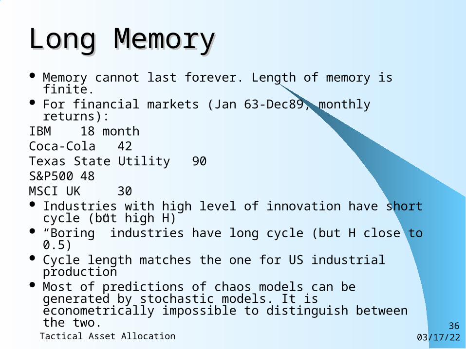
Long MemoryLong Memory Memory cannot last forever. Length of memory is finite. For financial markets (Jan 63-Dec89, monthly returns):IBM 18 monthCoca-Cola 42Texas State Utility 90S&P500 48MSCI UK 30 Industries with high level of innovation have short cycle (but
high H) “Boring” industries have long cycle (but H close to 0.5) Cycle length matches the one for US industrial production Most of predictions of chaos models can be generated by
stochastic models. It is econometrically impossible to distinguish between the two.
04/18/23Tactical Asset Allocation37
Correlations and Volatility:Correlations and Volatility: Predictable. Important in asset management Can be used in building dynamic trading strategy
(“vol trading”) Correlation forecasting is of somewhat limited
importance in “classical TAA”, difference with static returns is rather small.
Pecking order: expected returns, volatility, everything else…
Good model: EGARCH with a lot of dummies
04/18/23Tactical Asset Allocation38
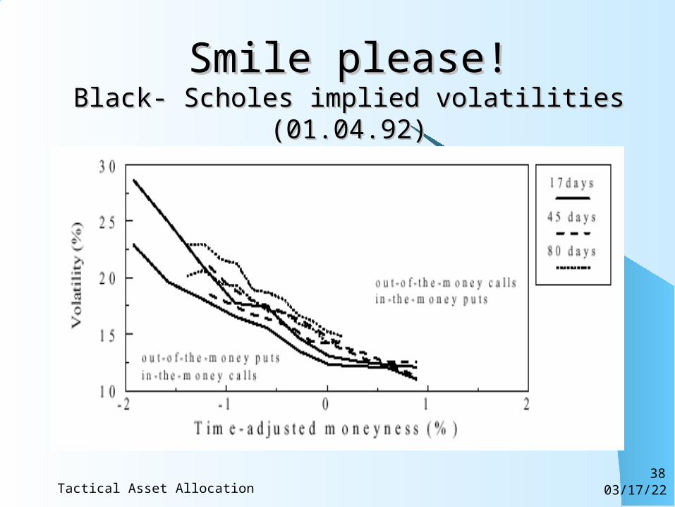
Smile please!Smile please!Black- Scholes implied volatilities (01.04.92)Black- Scholes implied volatilities (01.04.92)
04/18/23Tactical Asset Allocation39
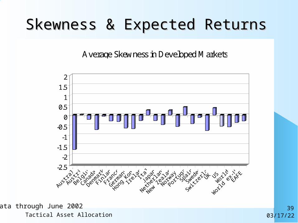
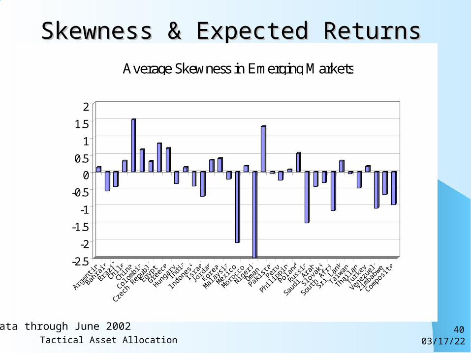
Skewness & Expected ReturnsSkewness & Expected Returns
-2.5
-2
-1.5
-1
-0.5
0
0.5
1
1.5
2
Australi
a
Austria
Belg
ium
Canad
a
Den
mar
k
Finlan
d
France
Ger
man
y
Hong K
ong
Irelan
d It
aly
Japan
Nether
lands
New
Zea
land
Norway
Portugal
Spain
Swed
en
Switzer
land UK US
World
World
ex-U
S
EAFE
Average Skewness in Developed Markets
Data through June 2002
04/18/23Tactical Asset Allocation40
Skewness & Expected ReturnsSkewness & Expected Returns
-2.5
-2
-1.5
-1
-0.5
0
0.5
1
1.5
2
Argen
tina
Bahrai
n
Brazil
Chile
China
Colombia
Czech
Rep
ublicEgy
pt
Greece
Hunga
ry
India
Indo
nesia
Israe
l
Jord
an
Korea
Mala
ysia
Mex
ico
Mor
occo
Nigeria
Oman
Pakist
an
Peru
Philipp
ines
Poland
Russia
Saudi
Arabia
Slovak
ia
South
Africa
Sri Lan
ka
Taiw
an
Thaila
nd
Turke
y
Venez
uela
Zimba
bwe
Compo
site
Average Skewness in Emerging Markets
Data through June 2002
04/18/23Tactical Asset Allocation41
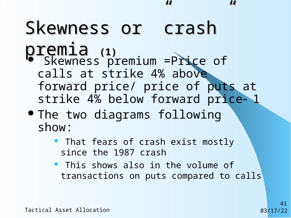
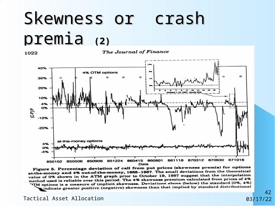
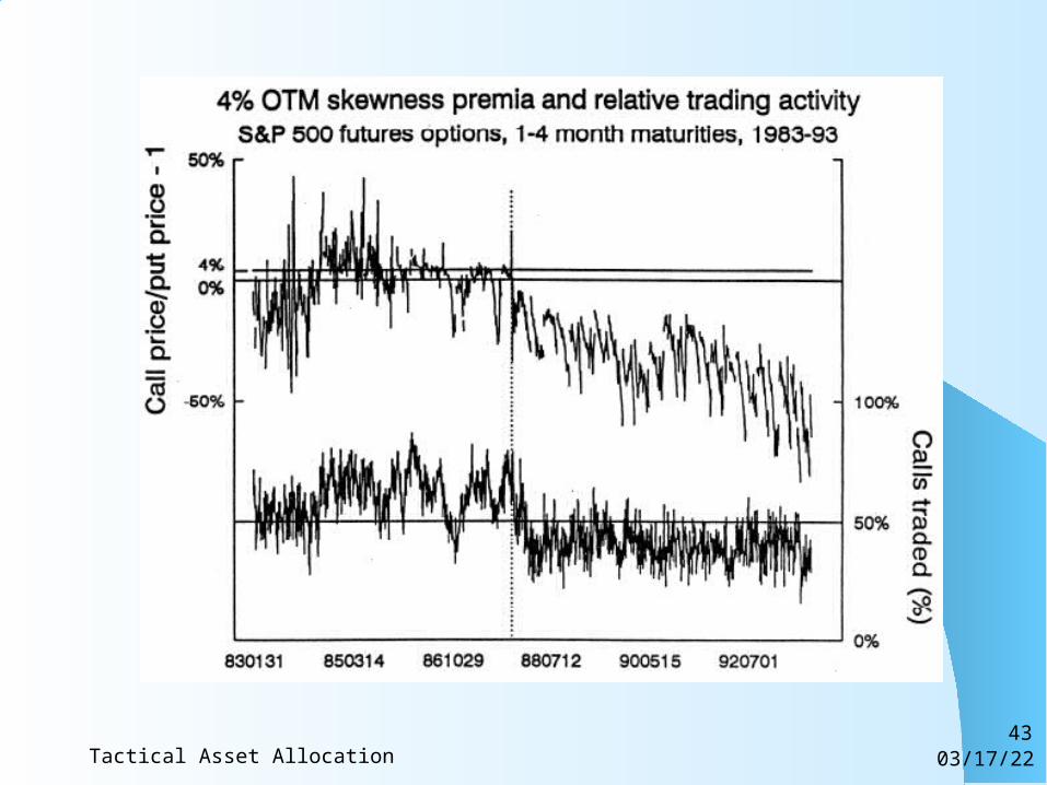
Skewness or ”crash” premia Skewness or ”crash” premia (1)(1)
Skewness premium =Price of calls at strike 4% above forward price/ price of puts at strike 4% below forward price1
The two diagrams following show:That fears of crash exist mostly since the 1987
crashThis shows also in the volume of transactions on
puts compared to calls
04/18/23Tactical Asset Allocation42
Skewness or ”crash” premia Skewness or ”crash” premia (2)(2)
04/18/23Tactical Asset Allocation43
04/18/23Tactical Asset Allocation44
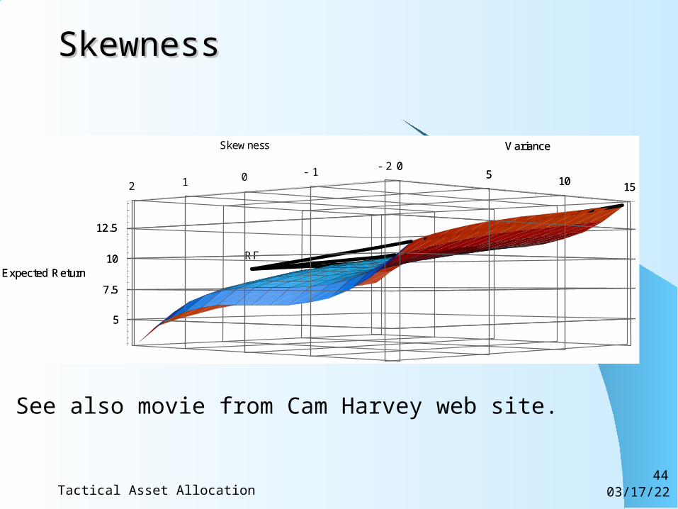
SkewnessSkewness
05 10 15
Variance
- 2- 1012
Skewness
5
7.5
10
12.5
Expected Return
RF
05 10 15
Variance
5
7.5
10
12.5
Expected Return
See also movie from Cam Harvey web site.
04/18/23Tactical Asset Allocation45
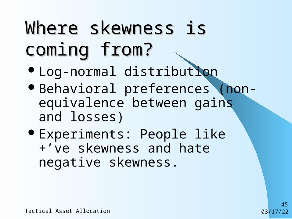
Where skewness is coming Where skewness is coming from?from?Log-normal distributionBehavioral preferences (non-equivalence
between gains and losses)Experiments: People like +’ve skewness
and hate negative skewness.
04/18/23Tactical Asset Allocation46
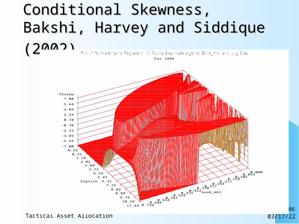
Conditional Skewness, Bakshi, Harvey Conditional Skewness, Bakshi, Harvey
and Siddique (2002)and Siddique (2002) For 1996
0. 7390. 686
0. 6340. 581
0. 5280. 475
0. 4220. 370
0. 3170. 264
0. 2110. 158
0. 1060. 053
0. 000
book_mkt
11. 4510. 59
9. 748. 88
8. 027. 16
6. 315. 45
4. 593. 73
2. 882. 02
1. 160. 31
- 0. 55
l ogs i ze
f 5s kew
- 7. 00
- 5. 44
- 3. 89
- 2. 33
- 0. 78
0. 78
2. 33
3. 89
5. 44
7. 00
04/18/23Tactical Asset Allocation47
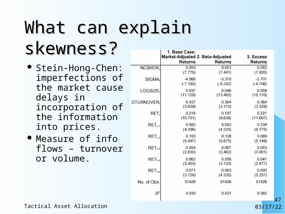
What can explain skewness?What can explain skewness?
Stein-Hong-Chen: imperfections of the market cause delays in incorporation of the information into prices.
Measure of info flows – turnover or volume.
04/18/23Tactical Asset Allocation48
Co-skewnessCo-skewness
Describe the probability of the assets to run-up or crash together.
Examples: ”Asian flu” of 98,” crashes in Eastern Europe after Russian Default.
Can be partially explained by the flows.Important: Try to avoid assets with +’ve
co-skewness. Especially important for hedge funds
Difficult to measure.
04/18/23Tactical Asset Allocation49
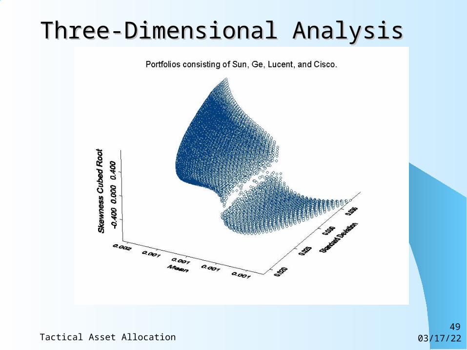
Three-Dimensional AnalysisThree-Dimensional Analysis
04/18/23Tactical Asset Allocation50
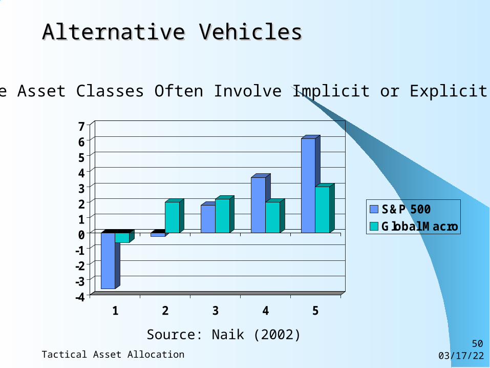
Alternative VehiclesAlternative Vehicles
Alternate Asset Classes Often Involve Implicit or Explicit Options
-4-3-2-101234567
1 2 3 4 5
S&P 500
Global Macro
Source: Naik (2002)
04/18/23Tactical Asset Allocation51
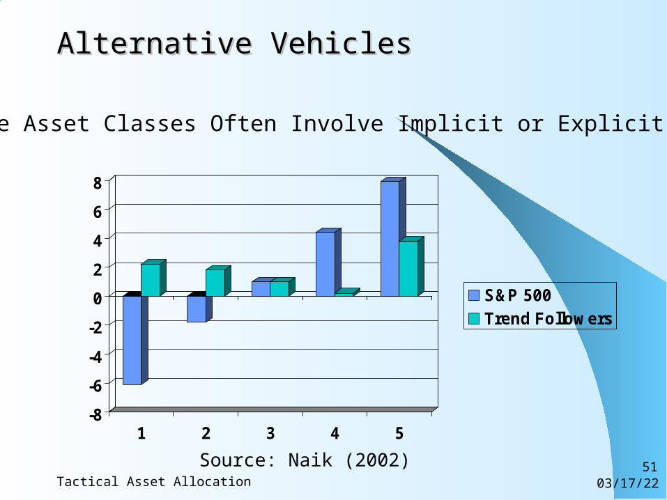
Alternative VehiclesAlternative Vehicles
Alternate Asset Classes Often Involve Implicit or Explicit Options
-8
-6
-4
-2
0
2
4
6
8
1 2 3 4 5
S&P 500
Trend Followers
Source: Naik (2002)
04/18/23Tactical Asset Allocation52
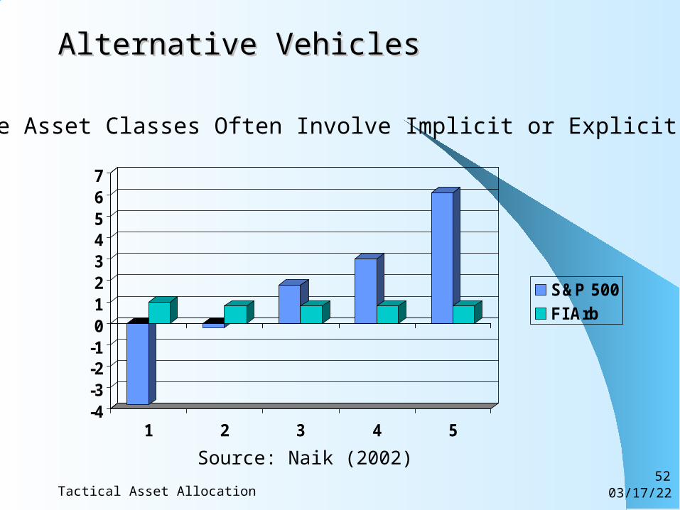
Alternative VehiclesAlternative Vehicles
Alternate Asset Classes Often Involve Implicit or Explicit Options
-4-3-2-101234567
1 2 3 4 5
S&P 500
FI Arb
Source: Naik (2002)
04/18/23Tactical Asset Allocation53
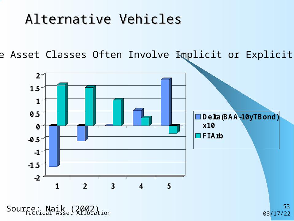
Alternative VehiclesAlternative Vehicles
Alternate Asset Classes Often Involve Implicit or Explicit Options
-2
-1.5
-1
-0.5
0
0.5
1
1.5
2
1 2 3 4 5
Delta(BAA-10yTBond)x10
FI Arb
Source: Naik (2002)
04/18/23Tactical Asset Allocation54
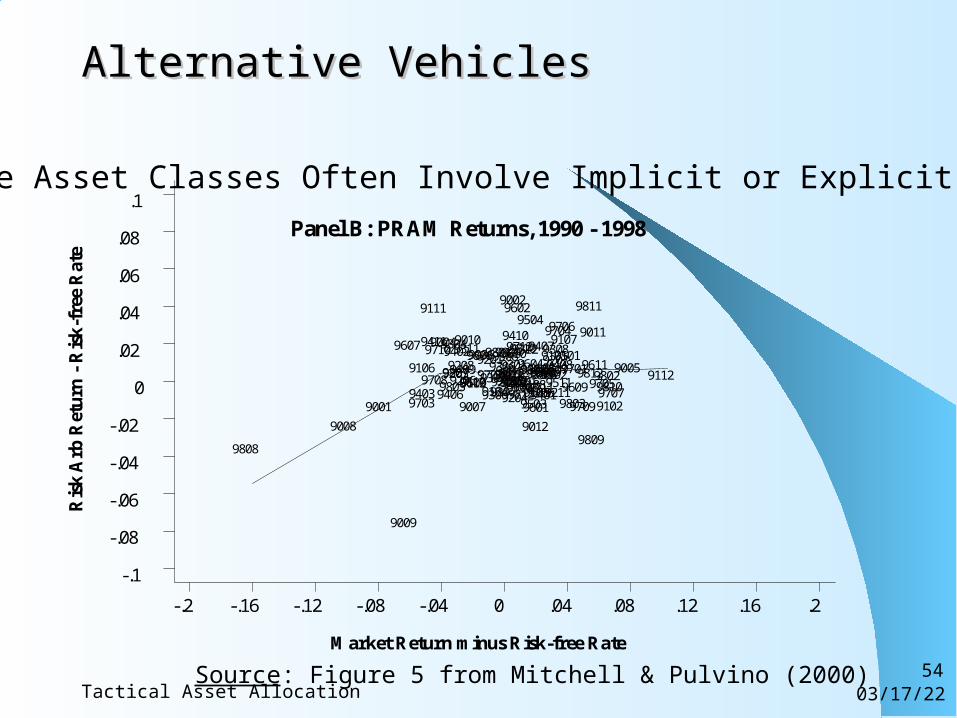
Alternative VehiclesAlternative Vehicles
Alternate Asset Classes Often Involve Implicit or Explicit Options
Panel B: PRAM Returns, 1990 - 1998
Ris
k A
rb R
etu
rn -
Ris
k-f
ree
Rat
e
Market Return minus Risk-free Rate
-.2 -.16 -.12 -.08 -.04 0 .04 .08 .12 .16 .2
-.1
-.08
-.06
-.04
-.02
0
.02
.04
.06
.08
.1
9808
9008
9001
9009
9607
9703
9106
9403
9111
9411
9708
97109004
94069805
9304
98079203
9402920892069409
93119010
9007
961295109109
9606900692019702930791049309
98019306
93029205
9508
9405
9804
9404960394129210
9002
9209
96109301951292029204
9410
9602
9110
9712
9212
9310
9501
9312
9003
9604
9504
9108
9503
96059303
9012
96019103
950697119305
9407
96089505
9401
980695099502
91059507
93089207
9211
9704
9511
9408
970691079101
9803
9701
9609
9709
9811
9812
9809
9011
9611
970598029810
91029707
90059112
Source: Figure 5 from Mitchell & Pulvino (2000)
04/18/23Tactical Asset Allocation55
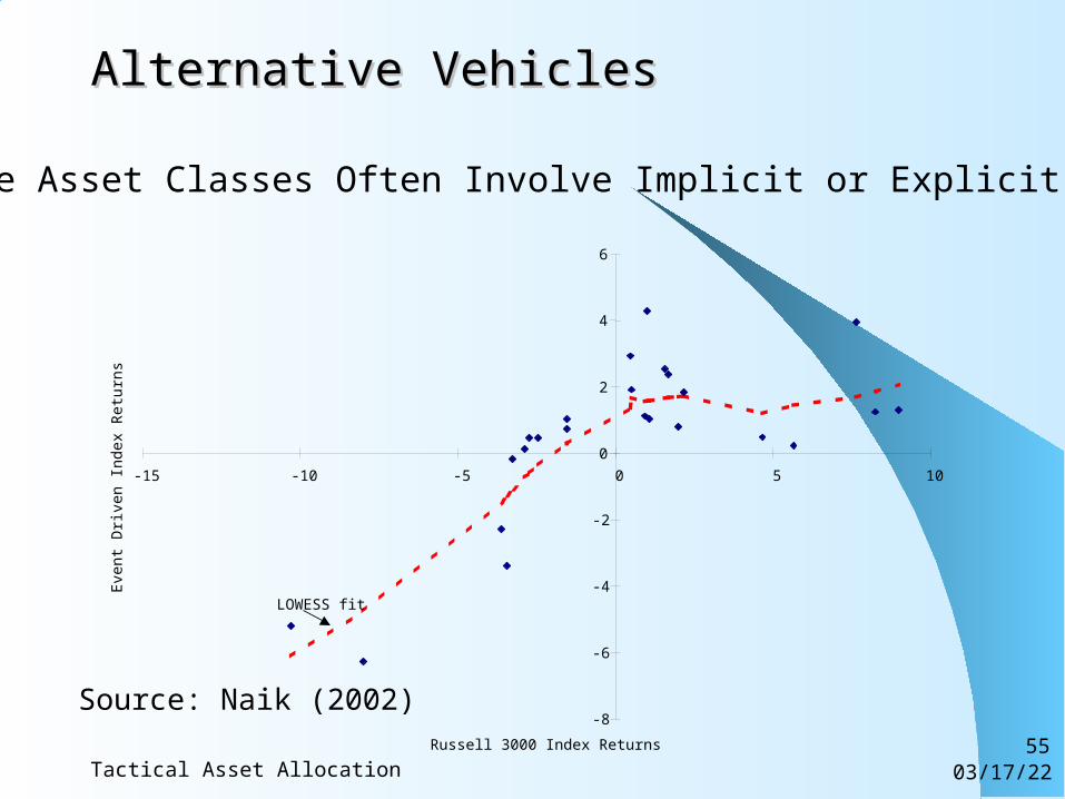
Alternative VehiclesAlternative Vehicles
Alternate Asset Classes Often Involve Implicit or Explicit Options
-8
-6
-4
-2
0
2
4
6
-15 -10 -5 0 5 10
Russell 3000 Index Returns
Eve
nt D
riven
Inde
x R
etur
ns
LOWESS fit
Source: Naik (2002)
04/18/23Tactical Asset Allocation56
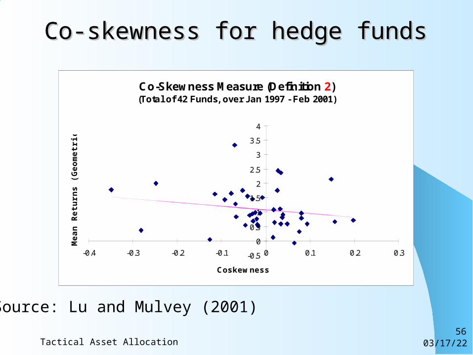
Co-skewness for hedge fundsCo-skewness for hedge funds
Co-Skewness Measure (Definition 2)(Total of 42 Funds, over Jan 1997 - Feb 2001)
-0.5
0
0.5
1
1.5
2
2.5
3
3.5
4
-0.4 -0.3 -0.2 -0.1 0 0.1 0.2 0.3
Coskewness
Mea
n R
etu
rns
(Geo
met
ric)
Source: Lu and Mulvey (2001)


