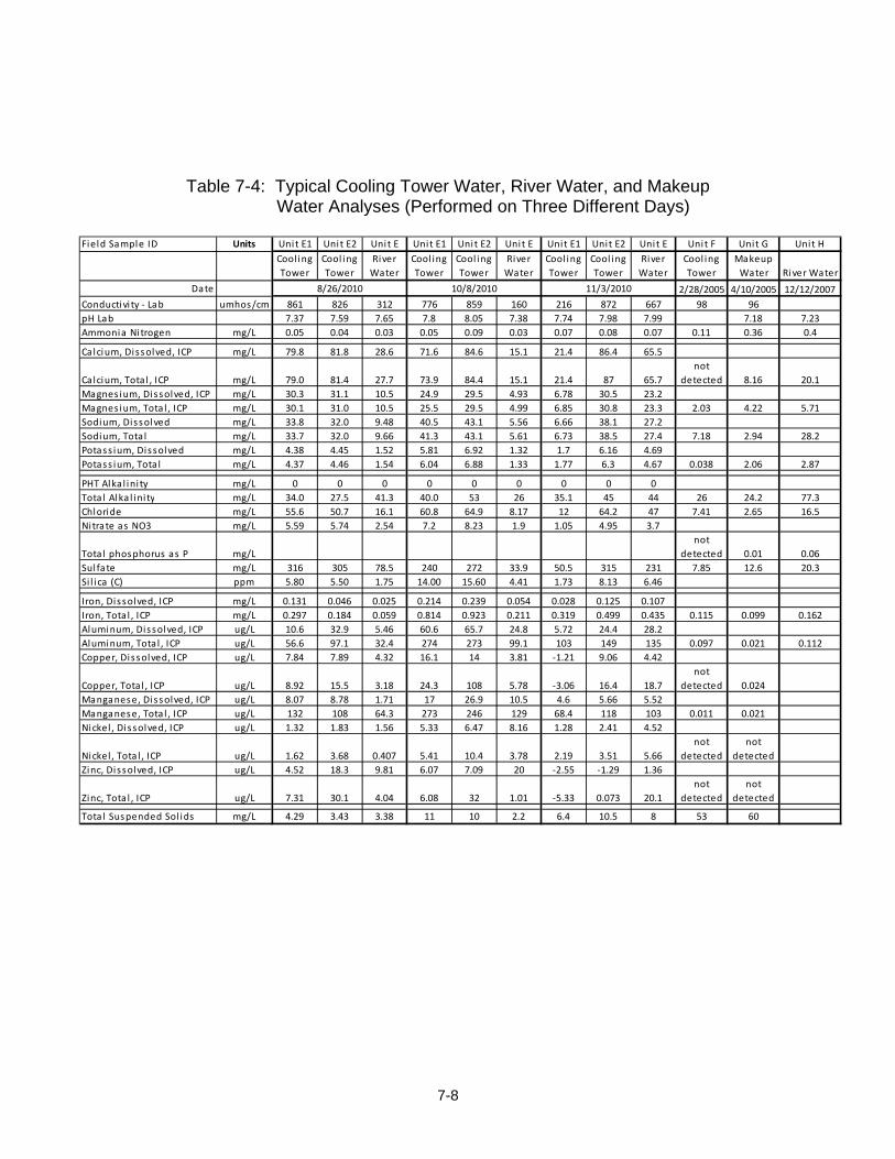
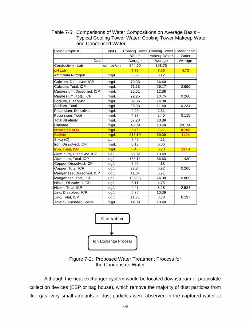
RECOVERY OF WATER FROM BOILER FLUE GAS USING CONDENSING HEAT EXCHANGERS FINAL TECHNICAL REPORT October 1, 2008 to March 31, 2011 by Edward Levy, Harun Bilirgen and John DuPont Report Issued June 2011 DOE Award Number DE-NT0005648 Energy Research Center Lehigh University 117 ATLSS Drive Bethlehem, PA 18015
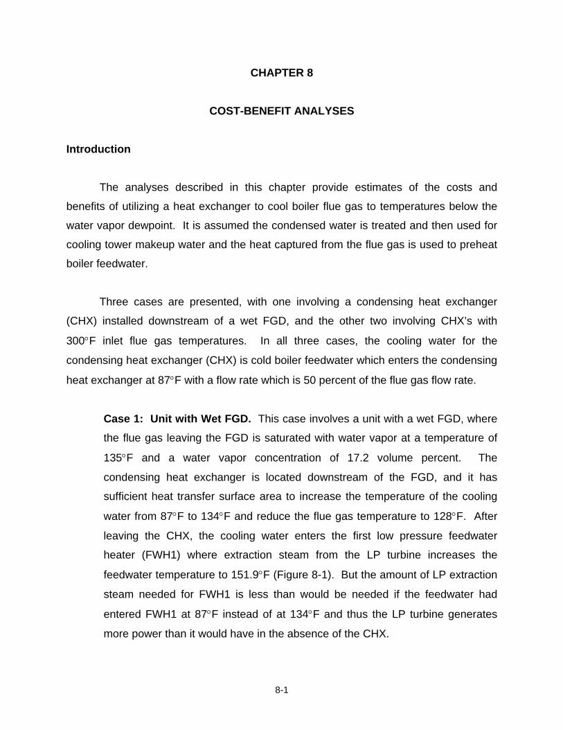
Transcript
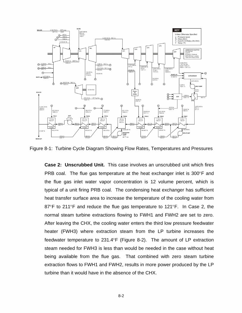
RECOVERY OF WATER FROM BOILER FLUE GAS USING CONDENSING HEAT EXCHANGERS
FINAL TECHNICAL REPORT
October 1, 2008 to March 31, 2011
by
Edward Levy, Harun Bilirgen and John DuPont
Report Issued June 2011
DOE Award Number DE-NT0005648
Energy Research Center Lehigh University 117 ATLSS Drive
Bethlehem, PA 18015
ii
DISCLAIMER
“This report was prepared as an account of work sponsored by an agency of the
United States Government. Neither the United States Government nor any agency
thereof, nor any of their employees, makes any warranty, express or implied, or
assumes any legal liability or responsibility for the accuracy, completeness, or
usefulness of any information, apparatus, product, or process disclosed, or represents
that its use would not infringe privately owned rights. Reference herein to any specific
commercial product, process, or service by trade name, trademark, manufacturer, or
otherwise does not necessarily constitute or imply its endorsement, recommendation, or
favoring by the United States Government or any agency thereof. The views and
opinions of authors expressed herein do not necessarily state or reflect those of the
United States Government or any agency thereof.”
iii
ACKNOWLEDGEMENTS In addition to the U.S. Department of Energy, the authors of this report are
extremely grateful to Southern Company and Lehigh University for supporting this
project.
The authors are also grateful to the other members of the Lehigh project team,
which included Dr. Hugo Caram and Messrs. Michael Kessen, Daniel Hazell, Jason
Thompson, Gordon Jonas, Nipun Goel, and Zheng Yao.
iv
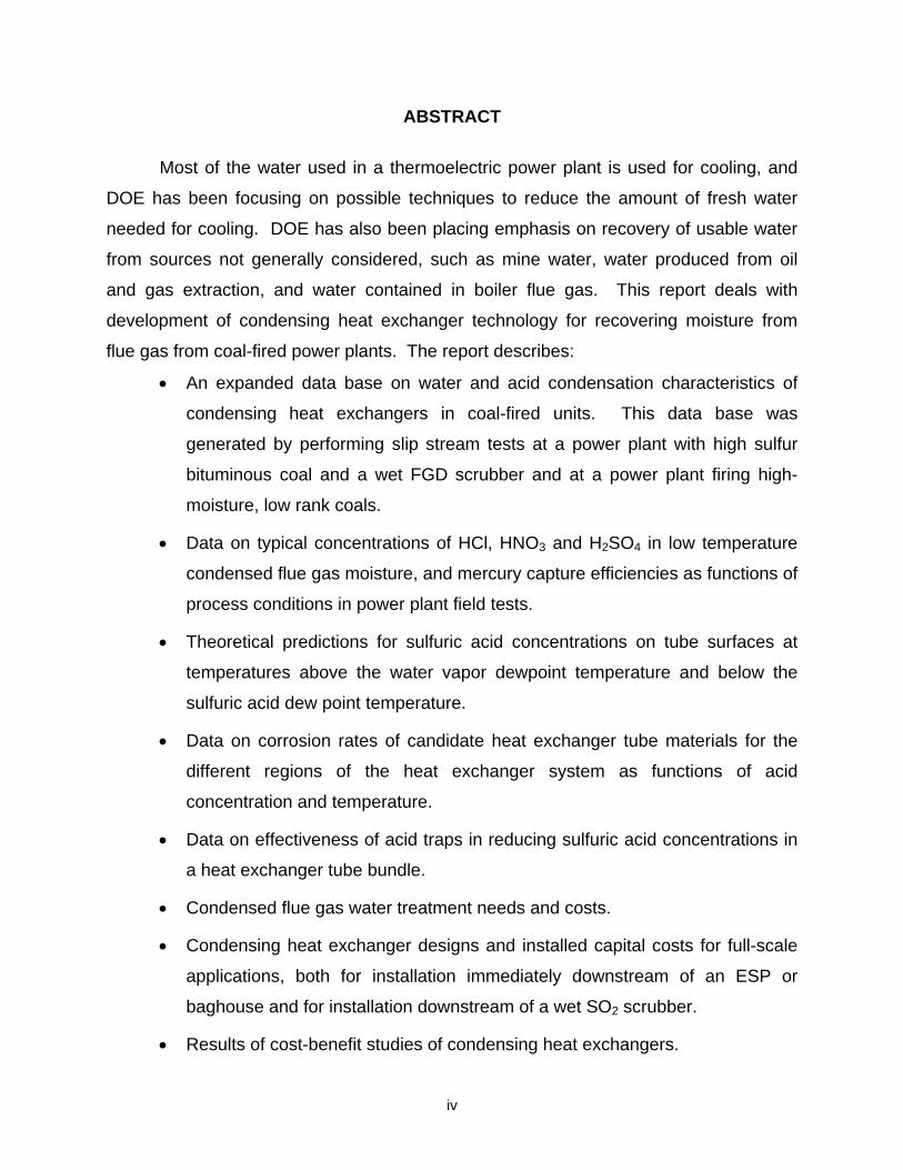
ABSTRACT Most of the water used in a thermoelectric power plant is used for cooling, and
DOE has been focusing on possible techniques to reduce the amount of fresh water
needed for cooling. DOE has also been placing emphasis on recovery of usable water
from sources not generally considered, such as mine water, water produced from oil
and gas extraction, and water contained in boiler flue gas. This report deals with
development of condensing heat exchanger technology for recovering moisture from
flue gas from coal-fired power plants. The report describes:
• An expanded data base on water and acid condensation characteristics of
condensing heat exchangers in coal-fired units. This data base was
generated by performing slip stream tests at a power plant with high sulfur
bituminous coal and a wet FGD scrubber and at a power plant firing high-
moisture, low rank coals.
• Data on typical concentrations of HCl, HNO3 and H2SO4 in low temperature
condensed flue gas moisture, and mercury capture efficiencies as functions of
process conditions in power plant field tests.
• Theoretical predictions for sulfuric acid concentrations on tube surfaces at
temperatures above the water vapor dewpoint temperature and below the
sulfuric acid dew point temperature.
• Data on corrosion rates of candidate heat exchanger tube materials for the
different regions of the heat exchanger system as functions of acid
concentration and temperature.
• Data on effectiveness of acid traps in reducing sulfuric acid concentrations in
a heat exchanger tube bundle.
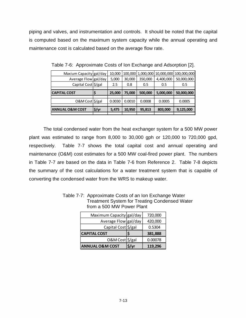
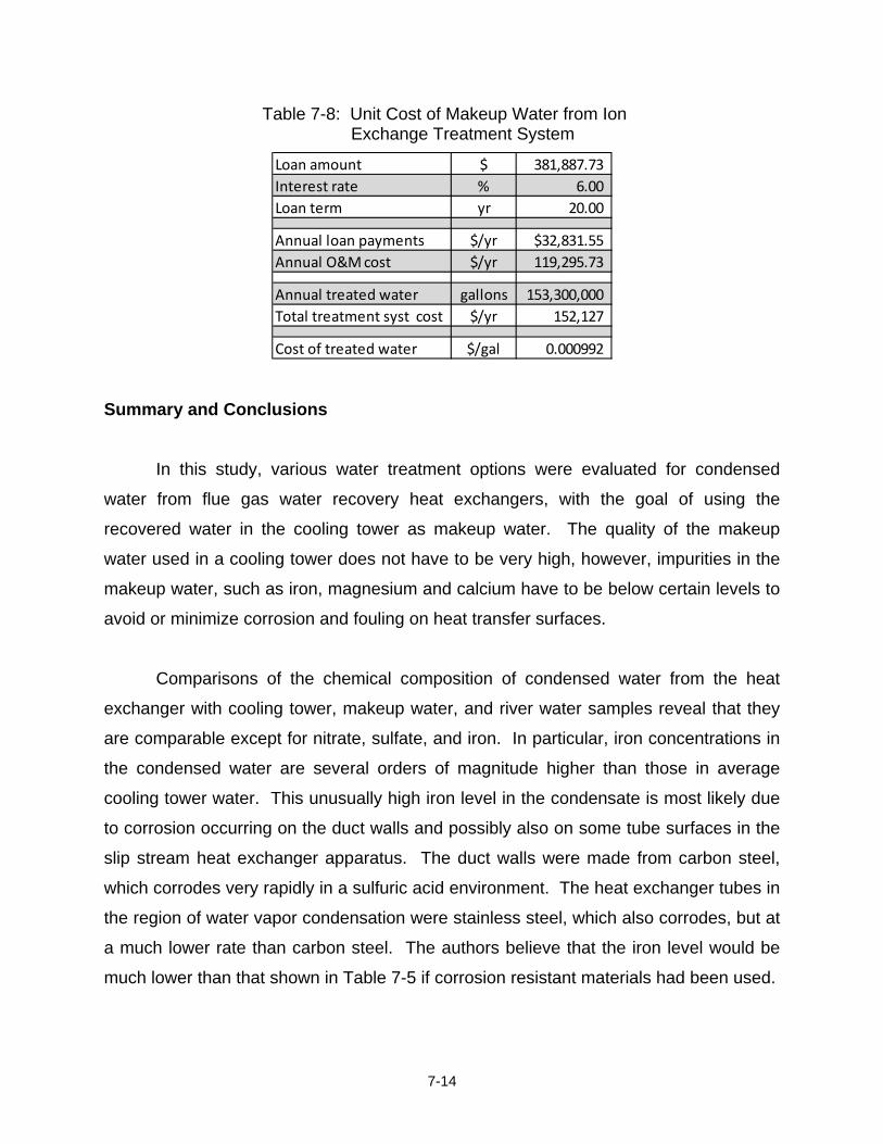
• Condensed flue gas water treatment needs and costs.
• Condensing heat exchanger designs and installed capital costs for full-scale
applications, both for installation immediately downstream of an ESP or
baghouse and for installation downstream of a wet SO2 scrubber.
• Results of cost-benefit studies of condensing heat exchangers.
v
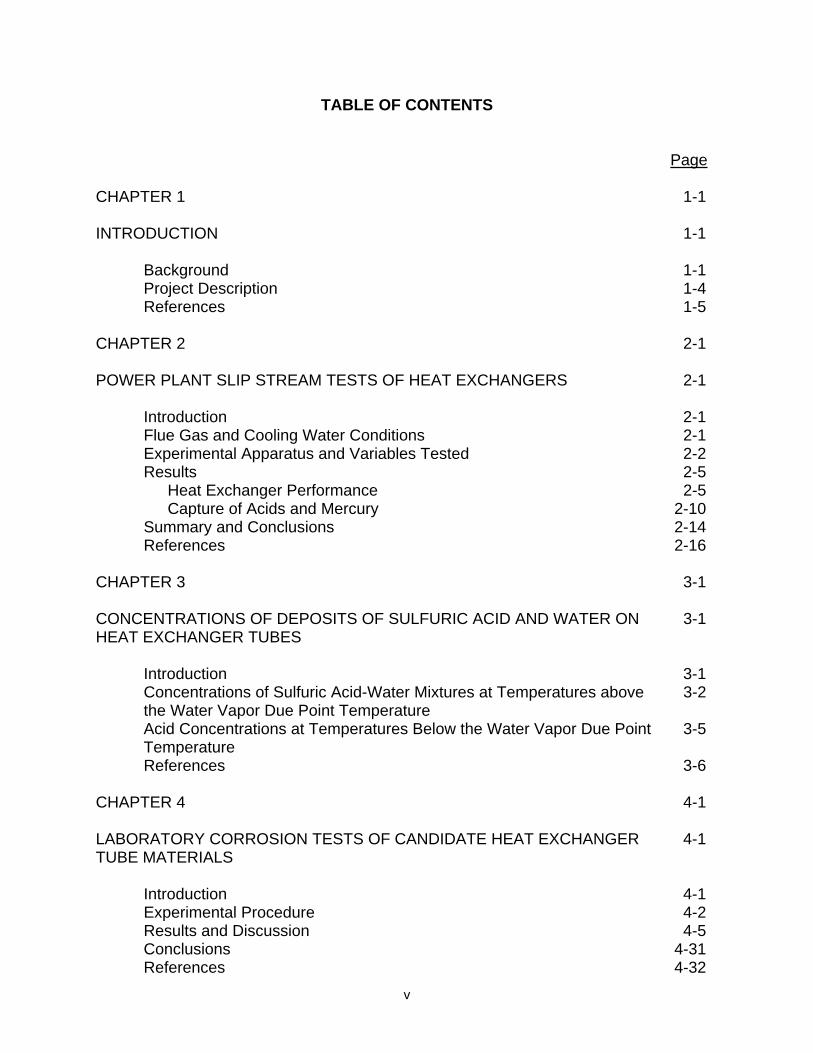
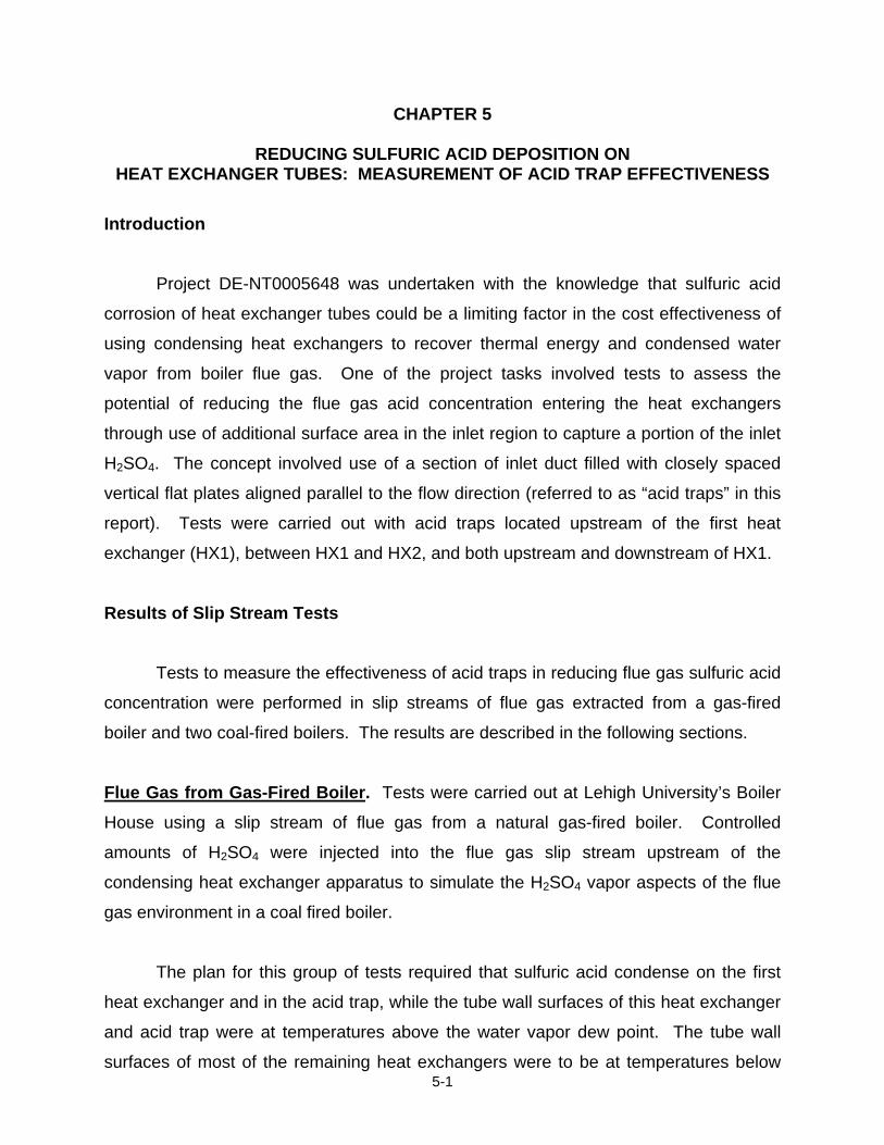
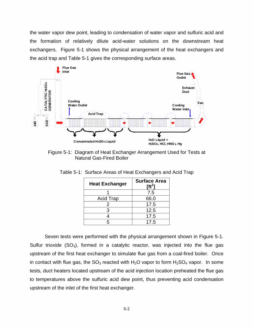
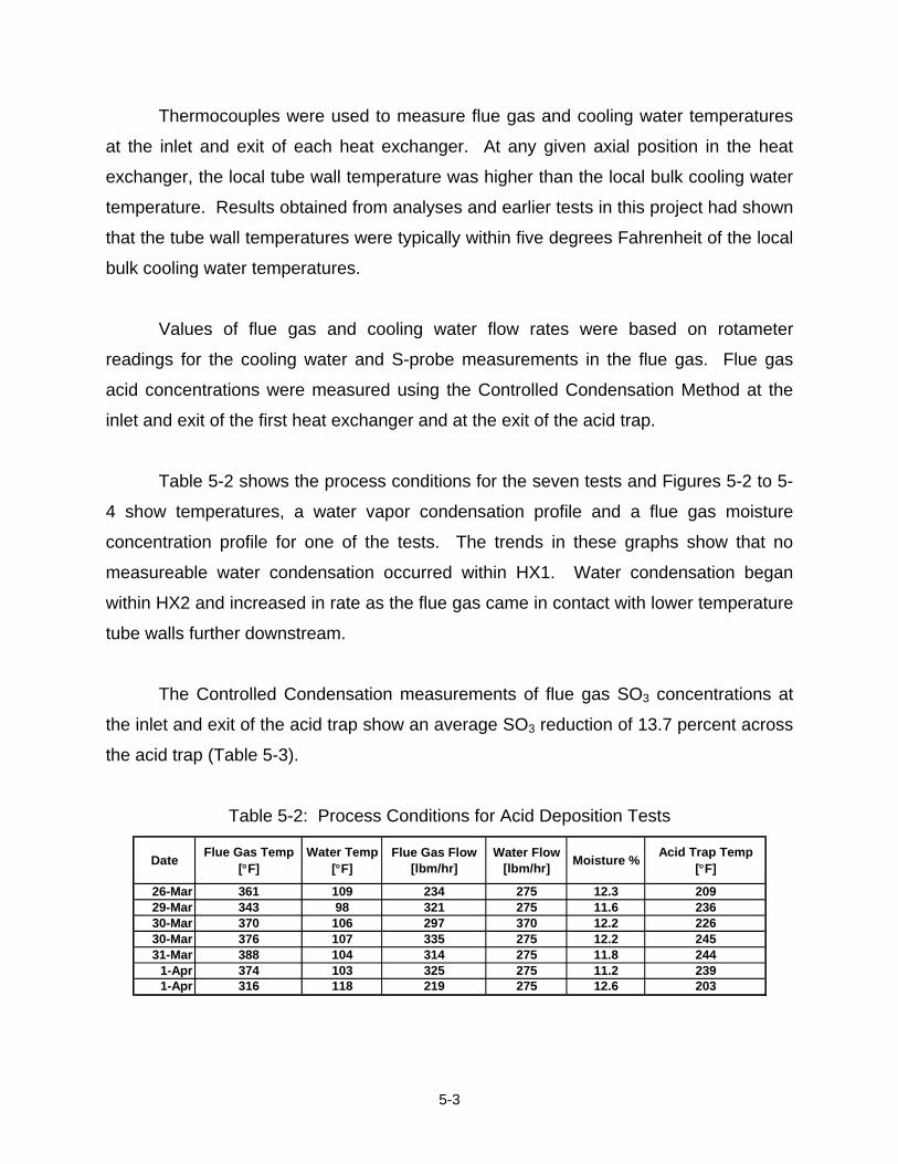
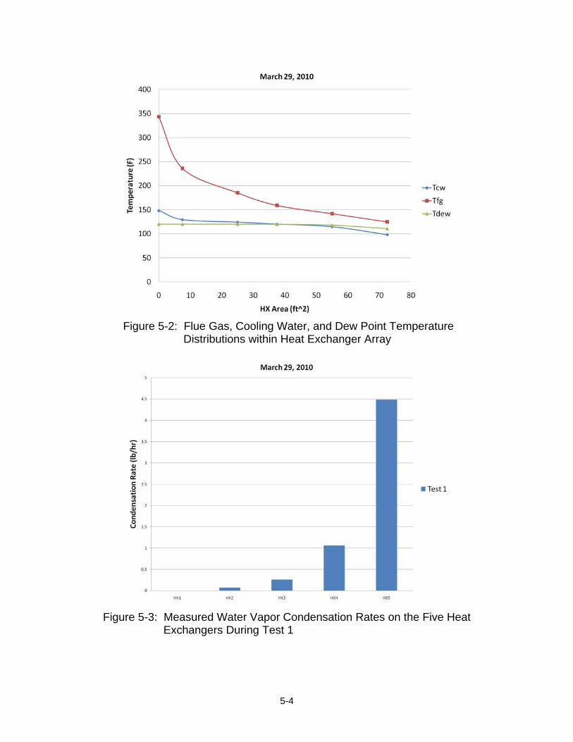
TABLE OF CONTENTS Page CHAPTER 1 1-1 INTRODUCTION 1-1 Background 1-1 Project Description 1-4 References 1-5 CHAPTER 2 2-1 POWER PLANT SLIP STREAM TESTS OF HEAT EXCHANGERS 2-1 Introduction 2-1 Flue Gas and Cooling Water Conditions 2-1 Experimental Apparatus and Variables Tested 2-2 Results 2-5 Heat Exchanger Performance 2-5 Capture of Acids and Mercury 2-10 Summary and Conclusions 2-14 References 2-16 CHAPTER 3 3-1 CONCENTRATIONS OF DEPOSITS OF SULFURIC ACID AND WATER ON 3-1 HEAT EXCHANGER TUBES Introduction 3-1 Concentrations of Sulfuric Acid-Water Mixtures at Temperatures above 3-2 the Water Vapor Due Point Temperature Acid Concentrations at Temperatures Below the Water Vapor Due Point 3-5 Temperature References 3-6 CHAPTER 4 4-1 LABORATORY CORROSION TESTS OF CANDIDATE HEAT EXCHANGER 4-1 TUBE MATERIALS Introduction 4-1 Experimental Procedure 4-2 Results and Discussion 4-5 Conclusions 4-31 References 4-32
vi
TABLE OF CONTENTS (continued)
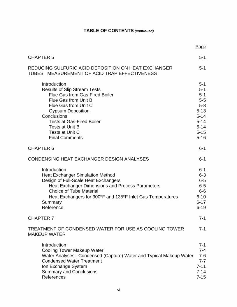
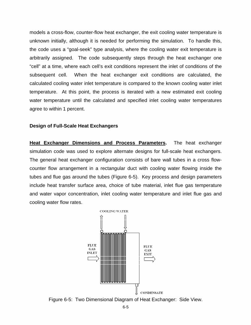
Page CHAPTER 5 5-1 REDUCING SULFURIC ACID DEPOSITION ON HEAT EXCHANGER 5-1 TUBES: MEASUREMENT OF ACID TRAP EFFECTIVENESS Introduction 5-1 Results of Slip Stream Tests 5-1 Flue Gas from Gas-Fired Boiler 5-1 Flue Gas from Unit B 5-5 Flue Gas from Unit C 5-8 Gypsum Deposition 5-13 Conclusions 5-14 Tests at Gas-Fired Boiler 5-14 Tests at Unit B 5-14 Tests at Unit C 5-15 Final Comments 5-16 CHAPTER 6 6-1 CONDENSING HEAT EXCHANGER DESIGN ANALYSES 6-1 Introduction 6-1 Heat Exchanger Simulation Method 6-3 Design of Full-Scale Heat Exchangers 6-5 Heat Exchanger Dimensions and Process Parameters 6-5 Choice of Tube Material 6-6 Heat Exchangers for 300°F and 135°F Inlet Gas Temperatures 6-10 Summary 6-17 Reference 6-19 CHAPTER 7 7-1 TREATMENT OF CONDENSED WATER FOR USE AS COOLING TOWER 7-1 MAKEUP WATER Introduction 7-1 Cooling Tower Makeup Water 7-4 Water Analyses: Condensed (Capture) Water and Typical Makeup Water 7-6 Condensed Water Treatment 7-7 Ion Exchange System 7-11 Summary and Conclusions 7-14 References 7-15
vii
TABLE OF CONTENTS (continued)
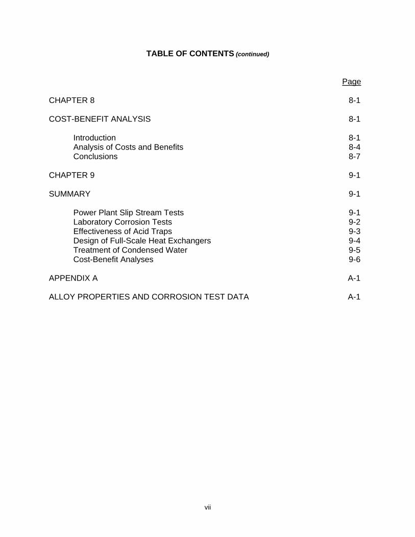
Page CHAPTER 8 8-1 COST-BENEFIT ANALYSIS 8-1 Introduction 8-1 Analysis of Costs and Benefits 8-4 Conclusions 8-7 CHAPTER 9 9-1 SUMMARY 9-1 Power Plant Slip Stream Tests 9-1 Laboratory Corrosion Tests 9-2 Effectiveness of Acid Traps 9-3 Design of Full-Scale Heat Exchangers 9-4 Treatment of Condensed Water 9-5 Cost-Benefit Analyses 9-6 APPENDIX A A-1 ALLOY PROPERTIES AND CORROSION TEST DATA A-1
viii
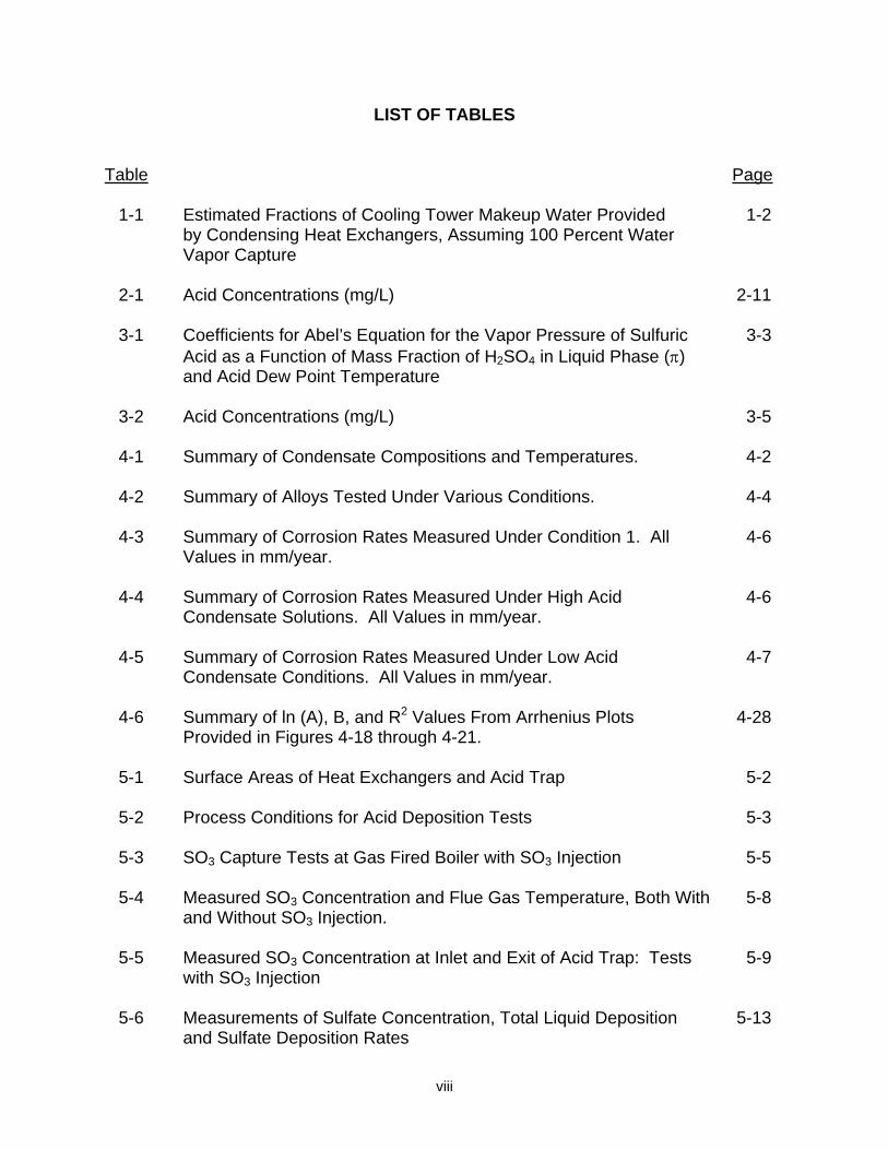
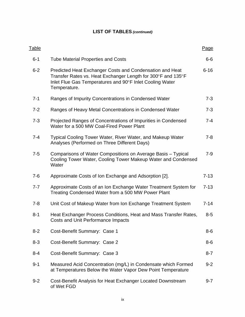
LIST OF TABLES
Table Page 1-1 Estimated Fractions of Cooling Tower Makeup Water Provided 1-2 by Condensing Heat Exchangers, Assuming 100 Percent Water Vapor Capture 2-1 Acid Concentrations (mg/L) 2-11 3-1 Coefficients for Abel’s Equation for the Vapor Pressure of Sulfuric 3-3
Acid as a Function of Mass Fraction of H2SO4 in Liquid Phase (π) and Acid Dew Point Temperature
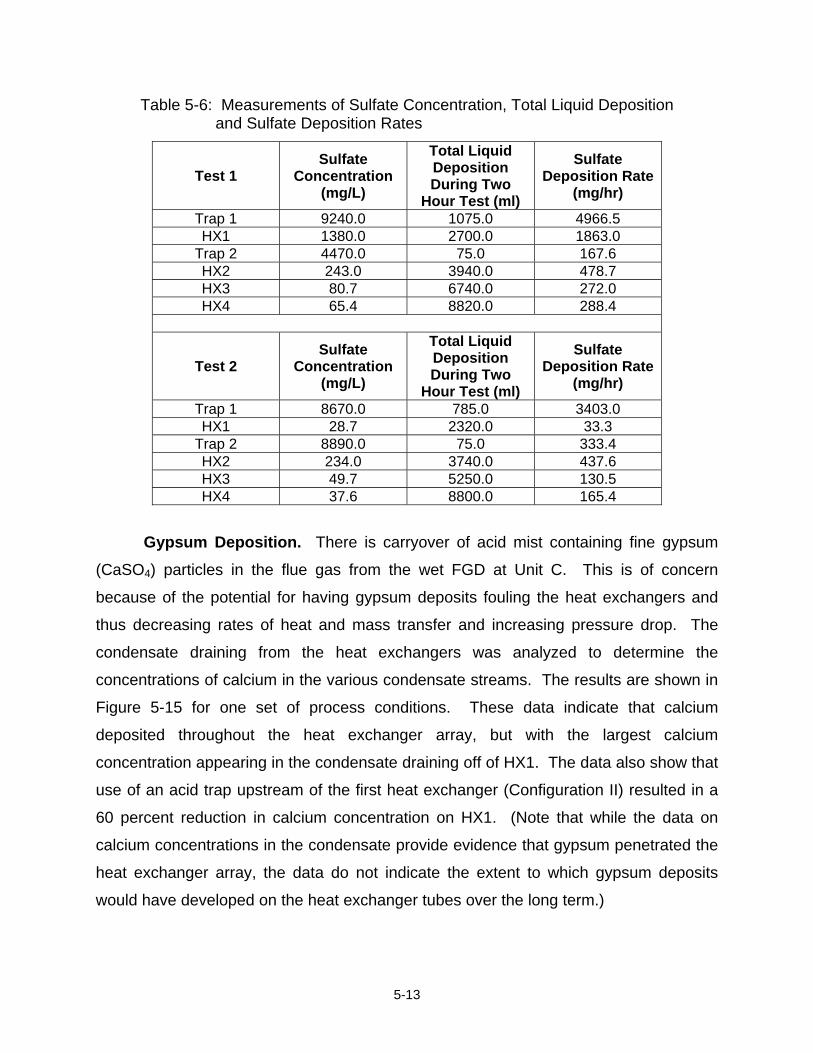
3-2 Acid Concentrations (mg/L) 3-5 4-1 Summary of Condensate Compositions and Temperatures. 4-2 4-2 Summary of Alloys Tested Under Various Conditions. 4-4 4-3 Summary of Corrosion Rates Measured Under Condition 1. All 4-6 Values in mm/year. 4-4 Summary of Corrosion Rates Measured Under High Acid 4-6 Condensate Solutions. All Values in mm/year. 4-5 Summary of Corrosion Rates Measured Under Low Acid 4-7 Condensate Conditions. All Values in mm/year. 4-6 Summary of ln (A), B, and R2 Values From Arrhenius Plots 4-28 Provided in Figures 4-18 through 4-21. 5-1 Surface Areas of Heat Exchangers and Acid Trap 5-2 5-2 Process Conditions for Acid Deposition Tests 5-3 5-3 SO3 Capture Tests at Gas Fired Boiler with SO3 Injection 5-5 5-4 Measured SO3 Concentration and Flue Gas Temperature, Both With 5-8 and Without SO3 Injection. 5-5 Measured SO3 Concentration at Inlet and Exit of Acid Trap: Tests 5-9 with SO3 Injection 5-6 Measurements of Sulfate Concentration, Total Liquid Deposition 5-13 and Sulfate Deposition Rates
ix
LIST OF TABLES (continued)
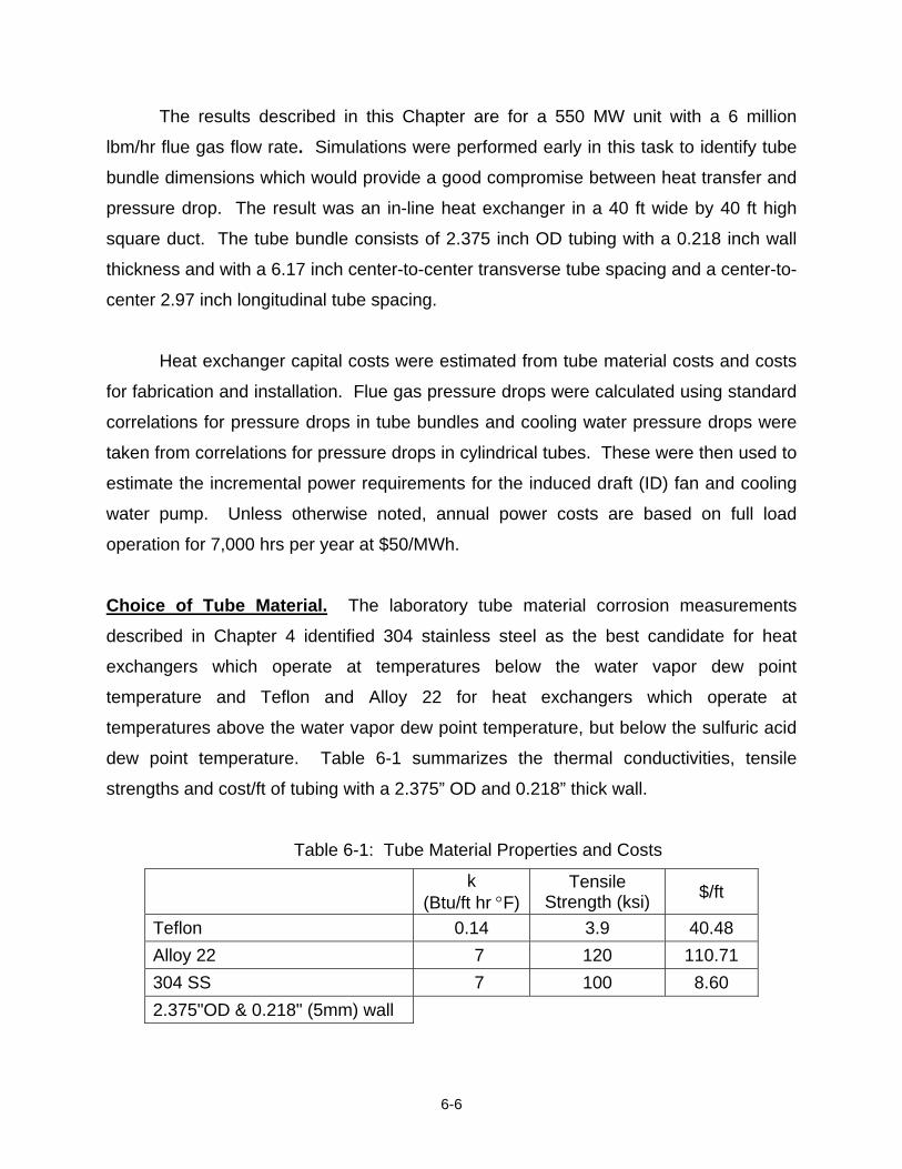
Table Page 6-1 Tube Material Properties and Costs 6-6 6-2 Predicted Heat Exchanger Costs and Condensation and Heat 6-16 Transfer Rates vs. Heat Exchanger Length for 300°F and 135°F Inlet Flue Gas Temperatures and 90°F Inlet Cooling Water Temperature. 7-1 Ranges of Impurity Concentrations in Condensed Water 7-3 7-2 Ranges of Heavy Metal Concentrations in Condensed Water 7-3 7-3 Projected Ranges of Concentrations of Impurities in Condensed 7-4 Water for a 500 MW Coal-Fired Power Plant 7-4 Typical Cooling Tower Water, River Water, and Makeup Water 7-8 Analyses (Performed on Three Different Days) 7-5 Comparisons of Water Compositions on Average Basis – Typical 7-9 Cooling Tower Water, Cooling Tower Makeup Water and Condensed Water 7-6 Approximate Costs of Ion Exchange and Adsorption [2]. 7-13 7-7 Approximate Costs of an Ion Exchange Water Treatment System for 7-13 Treating Condensed Water from a 500 MW Power Plant 7-8 Unit Cost of Makeup Water from Ion Exchange Treatment System 7-14 8-1 Heat Exchanger Process Conditions, Heat and Mass Transfer Rates, 8-5 Costs and Unit Performance Impacts 8-2 Cost-Benefit Summary: Case 1 8-6 8-3 Cost-Benefit Summary: Case 2 8-6 8-4 Cost-Benefit Summary: Case 3 8-7 9-1 Measured Acid Concentration (mg/L) in Condensate which Formed 9-2 at Temperatures Below the Water Vapor Dew Point Temperature 9-2 Cost-Benefit Analysis for Heat Exchanger Located Downstream 9-7 of Wet FGD
x
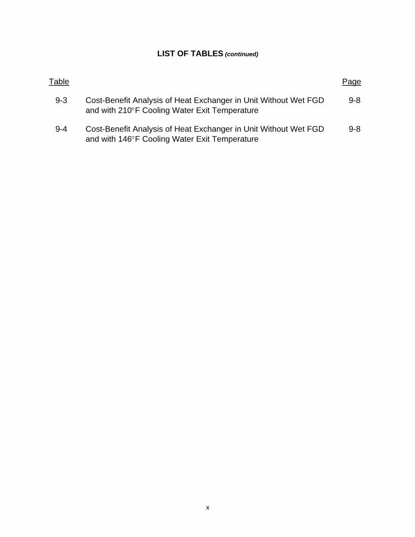
LIST OF TABLES (continued)
Table Page 9-3 Cost-Benefit Analysis of Heat Exchanger in Unit Without Wet FGD 9-8 and with 210°F Cooling Water Exit Temperature 9-4 Cost-Benefit Analysis of Heat Exchanger in Unit Without Wet FGD 9-8 and with 146°F Cooling Water Exit Temperature
xi
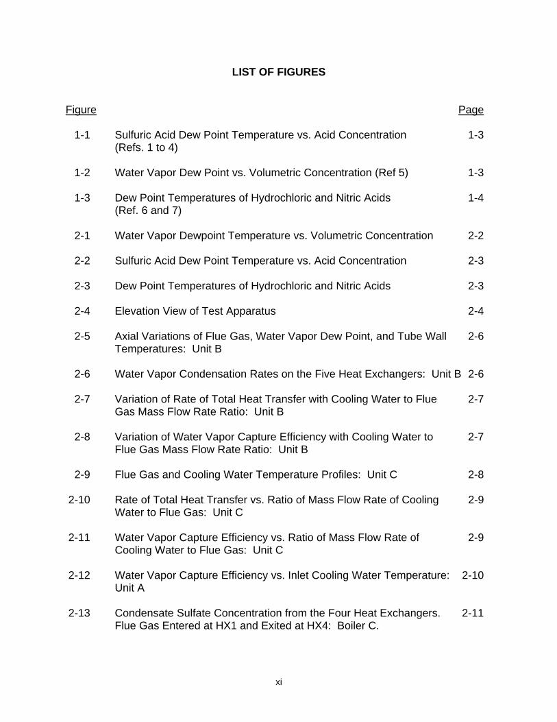
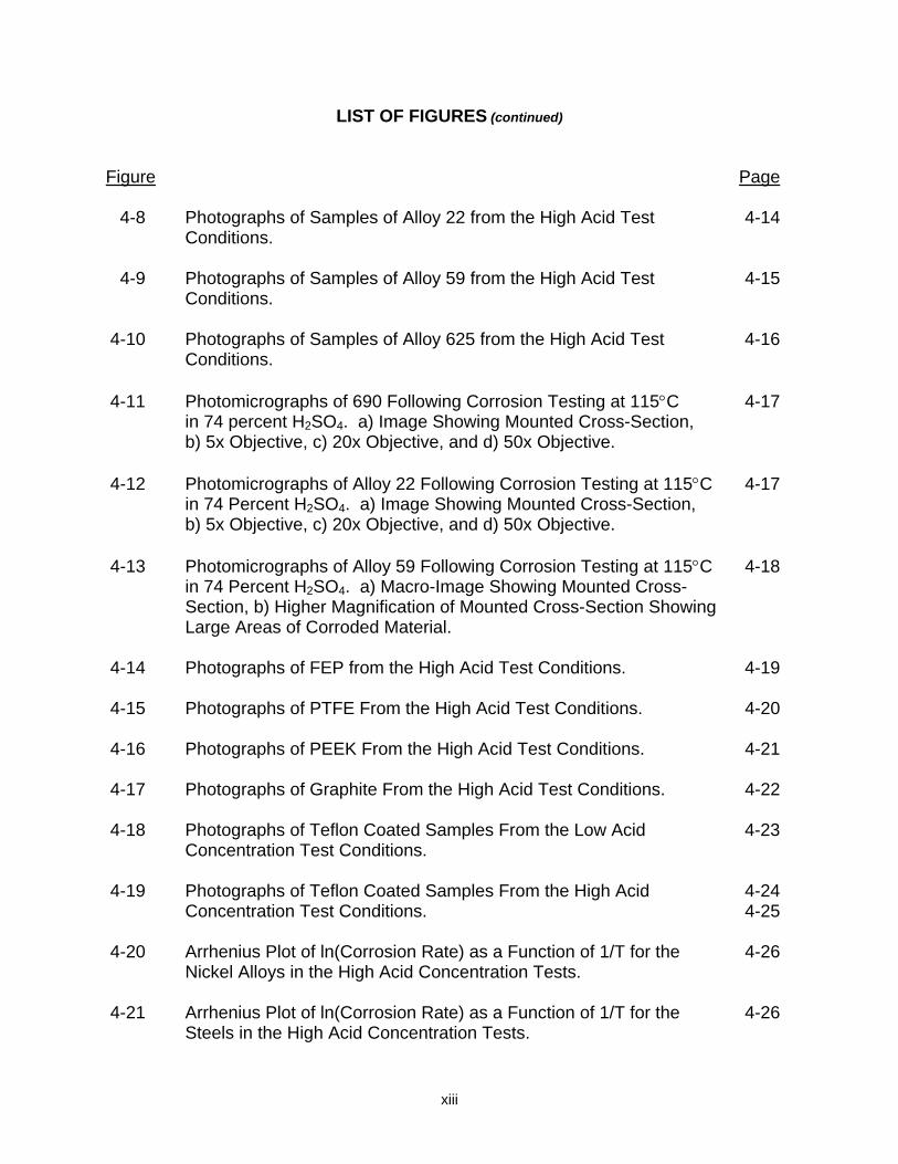
LIST OF FIGURES
Figure Page 1-1 Sulfuric Acid Dew Point Temperature vs. Acid Concentration 1-3 (Refs. 1 to 4) 1-2 Water Vapor Dew Point vs. Volumetric Concentration (Ref 5) 1-3 1-3 Dew Point Temperatures of Hydrochloric and Nitric Acids 1-4 (Ref. 6 and 7) 2-1 Water Vapor Dewpoint Temperature vs. Volumetric Concentration 2-2 2-2 Sulfuric Acid Dew Point Temperature vs. Acid Concentration 2-3 2-3 Dew Point Temperatures of Hydrochloric and Nitric Acids 2-3 2-4 Elevation View of Test Apparatus 2-4 2-5 Axial Variations of Flue Gas, Water Vapor Dew Point, and Tube Wall 2-6 Temperatures: Unit B 2-6 Water Vapor Condensation Rates on the Five Heat Exchangers: Unit B 2-6 2-7 Variation of Rate of Total Heat Transfer with Cooling Water to Flue 2-7 Gas Mass Flow Rate Ratio: Unit B 2-8 Variation of Water Vapor Capture Efficiency with Cooling Water to 2-7 Flue Gas Mass Flow Rate Ratio: Unit B 2-9 Flue Gas and Cooling Water Temperature Profiles: Unit C 2-8 2-10 Rate of Total Heat Transfer vs. Ratio of Mass Flow Rate of Cooling 2-9 Water to Flue Gas: Unit C 2-11 Water Vapor Capture Efficiency vs. Ratio of Mass Flow Rate of 2-9 Cooling Water to Flue Gas: Unit C 2-12 Water Vapor Capture Efficiency vs. Inlet Cooling Water Temperature: 2-10 Unit A 2-13 Condensate Sulfate Concentration from the Four Heat Exchangers. 2-11 Flue Gas Entered at HX1 and Exited at HX4: Boiler C.
xii
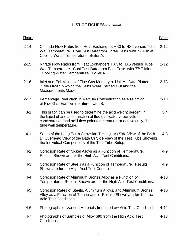
LIST OF FIGURES (continued)
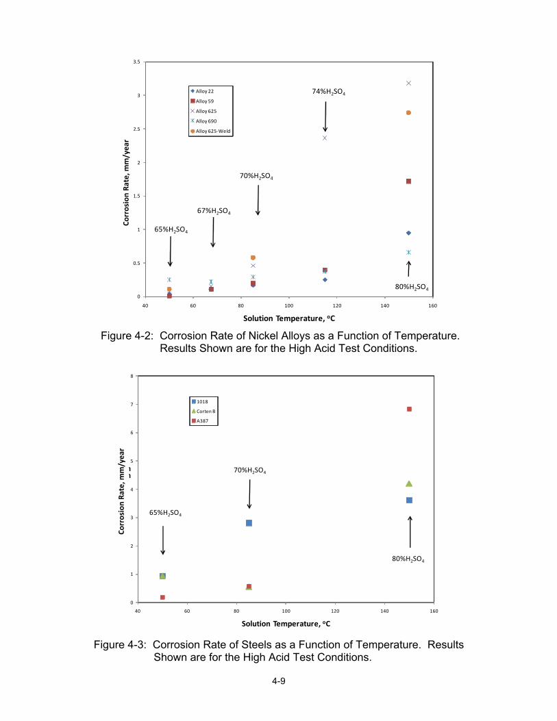
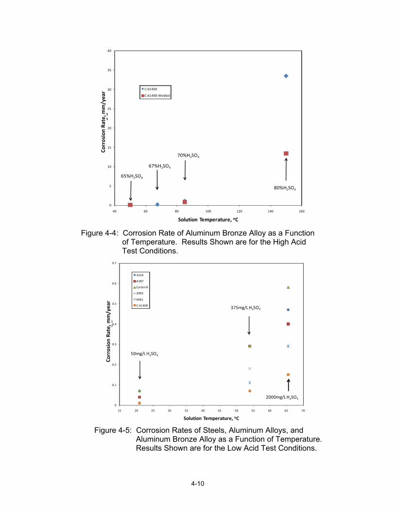
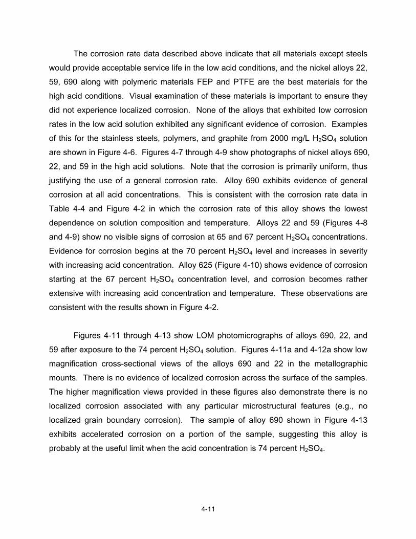
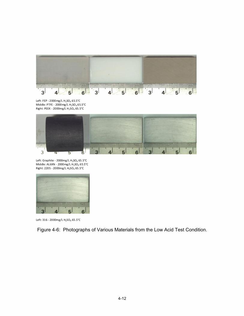
Figure Page 2-14 Chloride Flow Rates from Heat Exchangers HX3 to HX6 versus Tube 2-12 Wall Temperature. Coal Test Data from Three Tests with 77°F Inlet Cooling Water Temperature. Boiler A. 2-15 Nitrate Flow Rates from Heat Exchangers HX3 to HX6 versus Tube 2-12 Wall Temperature. Coal Test Data from Four Tests with 77°F Inlet Cooling Water Temperature. Boiler A. 2-16 Inlet and Exit Values of Flue Gas Mercury at Unit A. Data Plotted 2-13 in the Order in which the Tests Were Carried Out and the Measurements Made. 2-17 Percentage Reduction in Mercury Concentration as a Function 2-13 of Flue Gas Exit Temperature: Unit B. 3-1 This graph can be used to determine the acid weight percent in 3-4 the liquid phase as a function of flue gas water vapor volume concentration and acid dew point temperature, or equivalently, the tube wall temperature. 4-1 Setup of the Long-Term Corrosion Testing. A) Side View of the Bath 4-3 B) Overhead View of the Bath C) Side View of the Test Tube Showing the Individual Components of the Test Tube Setup. 4-2 Corrosion Rate of Nickel Alloys as a Function of Temperature. 4-9 Results Shown are for the High Acid Test Conditions. 4-3 Corrosion Rate of Steels as a Function of Temperature. Results 4-9 Shown are for the High Acid Test Conditions. 4-4 Corrosion Rate of Aluminum Bronze Alloy as a Function of 4-10 Temperature. Results Shown are for the High Acid Test Conditions. 4-5 Corrosion Rates of Steels, Aluminum Alloys, and Aluminum Bronze 4-10 Alloy as a Function of Temperature. Results Shown are for the Low Acid Test Conditions. 4-6 Photographs of Various Materials from the Low Acid Test Condition. 4-12 4-7 Photographs of Samples of Alloy 690 from the High Acid Test 4-13 Conditions.
xiii
LIST OF FIGURES (continued)
Figure Page 4-8 Photographs of Samples of Alloy 22 from the High Acid Test 4-14 Conditions. 4-9 Photographs of Samples of Alloy 59 from the High Acid Test 4-15 Conditions. 4-10 Photographs of Samples of Alloy 625 from the High Acid Test 4-16 Conditions. 4-11 Photomicrographs of 690 Following Corrosion Testing at 115°C 4-17 in 74 percent H2SO4. a) Image Showing Mounted Cross-Section, b) 5x Objective, c) 20x Objective, and d) 50x Objective. 4-12 Photomicrographs of Alloy 22 Following Corrosion Testing at 115°C 4-17 in 74 Percent H2SO4. a) Image Showing Mounted Cross-Section, b) 5x Objective, c) 20x Objective, and d) 50x Objective. 4-13 Photomicrographs of Alloy 59 Following Corrosion Testing at 115°C 4-18 in 74 Percent H2SO4. a) Macro-Image Showing Mounted Cross- Section, b) Higher Magnification of Mounted Cross-Section Showing Large Areas of Corroded Material. 4-14 Photographs of FEP from the High Acid Test Conditions. 4-19 4-15 Photographs of PTFE From the High Acid Test Conditions. 4-20 4-16 Photographs of PEEK From the High Acid Test Conditions. 4-21 4-17 Photographs of Graphite From the High Acid Test Conditions. 4-22 4-18 Photographs of Teflon Coated Samples From the Low Acid 4-23 Concentration Test Conditions. 4-19 Photographs of Teflon Coated Samples From the High Acid 4-24 Concentration Test Conditions. 4-25 4-20 Arrhenius Plot of ln(Corrosion Rate) as a Function of 1/T for the 4-26 Nickel Alloys in the High Acid Concentration Tests. 4-21 Arrhenius Plot of ln(Corrosion Rate) as a Function of 1/T for the 4-26 Steels in the High Acid Concentration Tests.
xiv
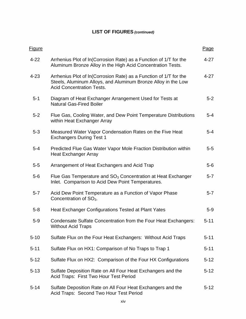
LIST OF FIGURES (continued)
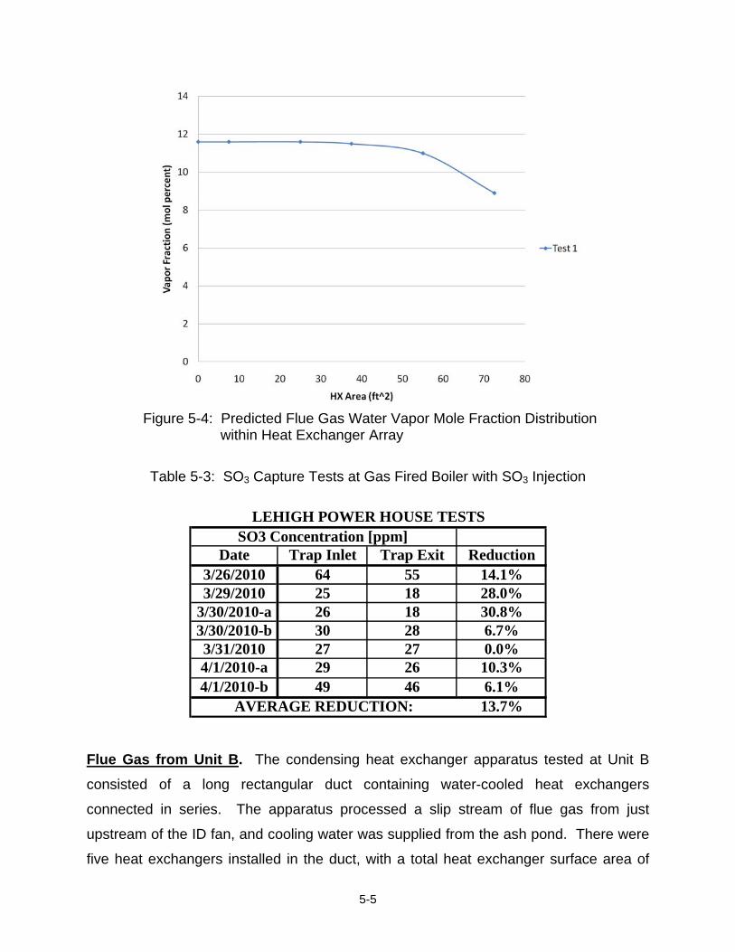
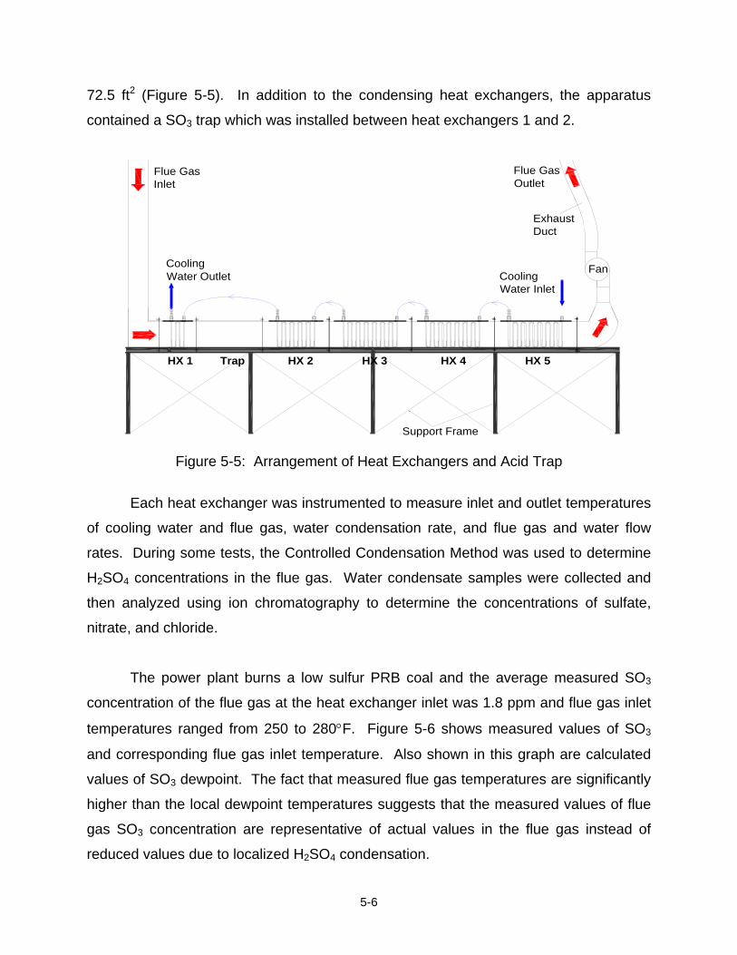
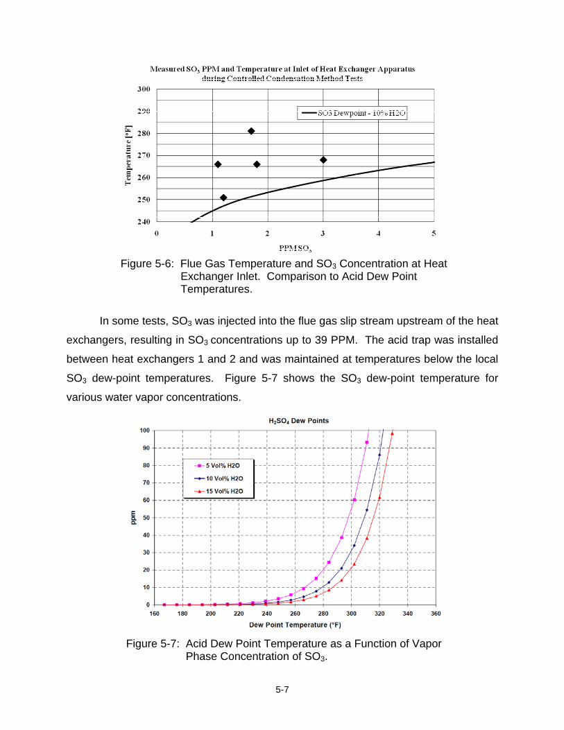
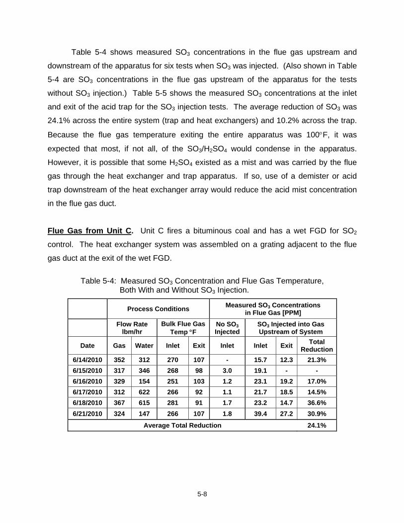
Figure Page 4-22 Arrhenius Plot of ln(Corrosion Rate) as a Function of 1/T for the 4-27 Aluminum Bronze Alloy in the High Acid Concentration Tests. 4-23 Arrhenius Plot of ln(Corrosion Rate) as a Function of 1/T for the 4-27 Steels, Aluminum Alloys, and Aluminum Bronze Alloy in the Low Acid Concentration Tests. 5-1 Diagram of Heat Exchanger Arrangement Used for Tests at 5-2 Natural Gas-Fired Boiler 5-2 Flue Gas, Cooling Water, and Dew Point Temperature Distributions 5-4 within Heat Exchanger Array 5-3 Measured Water Vapor Condensation Rates on the Five Heat 5-4 Exchangers During Test 1 5-4 Predicted Flue Gas Water Vapor Mole Fraction Distribution within 5-5 Heat Exchanger Array 5-5 Arrangement of Heat Exchangers and Acid Trap 5-6 5-6 Flue Gas Temperature and SO3 Concentration at Heat Exchanger 5-7 Inlet. Comparison to Acid Dew Point Temperatures. 5-7 Acid Dew Point Temperature as a Function of Vapor Phase 5-7 Concentration of SO3. 5-8 Heat Exchanger Configurations Tested at Plant Yates 5-9 5-9 Condensate Sulfate Concentration from the Four Heat Exchangers: 5-11 Without Acid Traps 5-10 Sulfate Flux on the Four Heat Exchangers: Without Acid Traps 5-11 5-11 Sulfate Flux on HX1: Comparison of No Traps to Trap 1 5-11 5-12 Sulfate Flux on HX2: Comparison of the Four HX Configurations 5-12 5-13 Sulfate Deposition Rate on All Four Heat Exchangers and the 5-12 Acid Traps: First Two Hour Test Period 5-14 Sulfate Deposition Rate on All Four Heat Exchangers and the 5-12 Acid Traps: Second Two Hour Test Period
xv
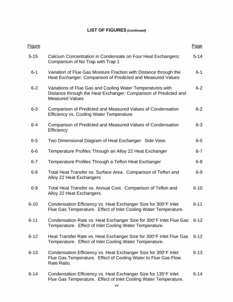
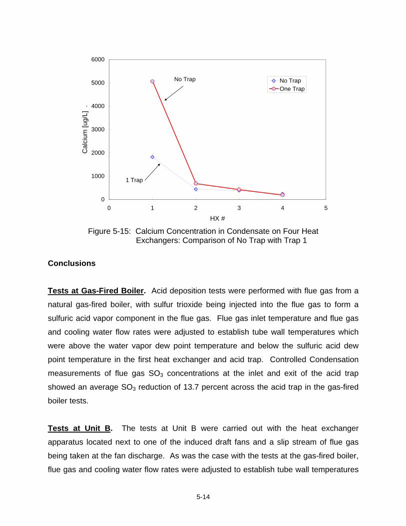
LIST OF FIGURES (continued)
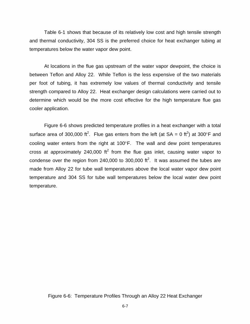
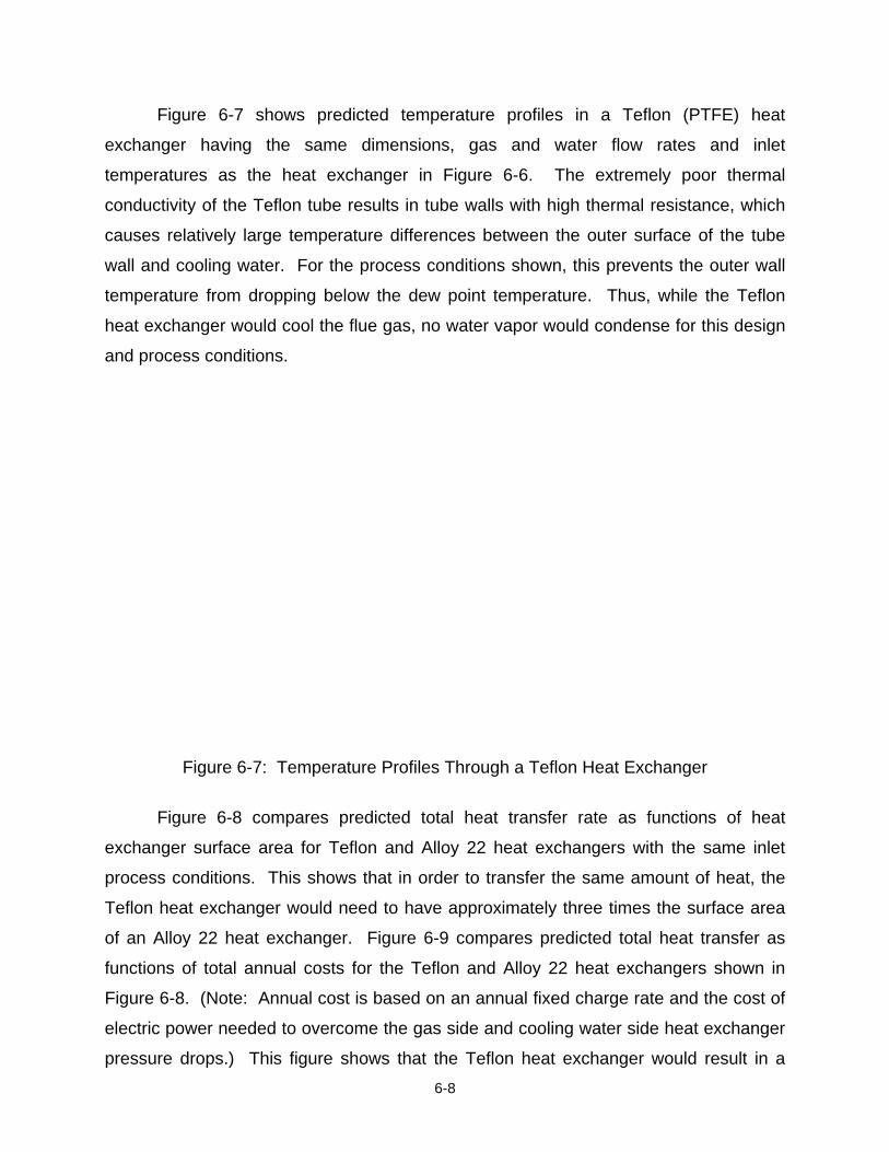
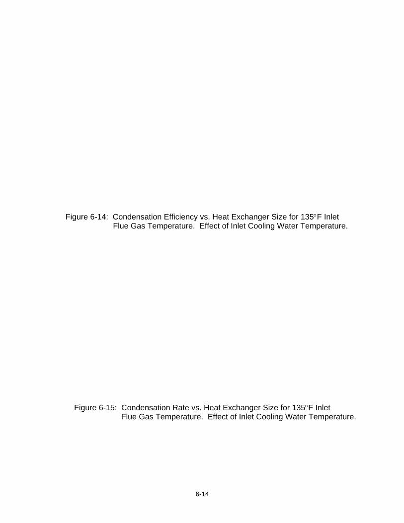
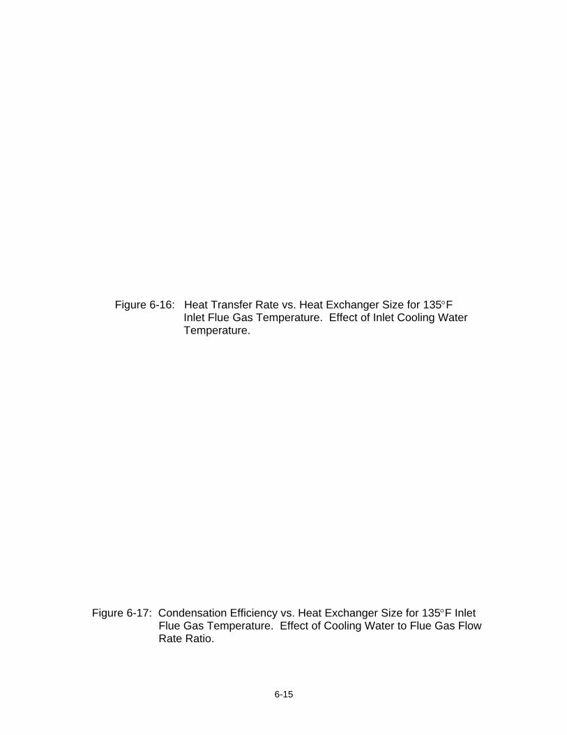
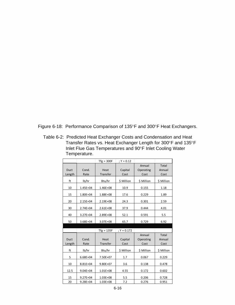
Figure Page 5-15 Calcium Concentration in Condensate on Four Heat Exchangers: 5-14 Comparison of No Trap with Trap 1 6-1 Variation of Flue Gas Moisture Fraction with Distance through the 6-1 Heat Exchanger: Comparison of Predicted and Measured Values 6-2 Variations of Flue Gas and Cooling Water Temperatures with 6-2 Distance through the Heat Exchanger: Comparison of Predicted and Measured Values 6-3 Comparison of Predicted and Measured Values of Condensation 6-2 Efficiency vs. Cooling Water Temperature 6-4 Comparison of Predicted and Measured Values of Condensation 6-3 Efficiency 6-5 Two Dimensional Diagram of Heat Exchanger: Side View. 6-5 6-6 Temperature Profiles Through an Alloy 22 Heat Exchanger 6-7 6-7 Temperature Profiles Through a Teflon Heat Exchanger 6-8 6-8 Total Heat Transfer vs. Surface Area. Comparison of Teflon and 6-9 Alloy 22 Heat Exchangers 6-9 Total Heat Transfer vs. Annual Cost. Comparison of Teflon and 6-10 Alloy 22 Heat Exchangers. 6-10 Condensation Efficiency vs. Heat Exchanger Size for 300°F Inlet 6-11 Flue Gas Temperature. Effect of Inlet Cooling Water Temperature. 6-11 Condensation Rate vs. Heat Exchanger Size for 300°F Inlet Flue Gas 6-12 Temperature. Effect of Inlet Cooling Water Temperature. 6-12 Heat Transfer Rate vs. Heat Exchanger Size for 300°F Inlet Flue Gas 6-12 Temperature. Effect of Inlet Cooling Water Temperature. 6-13 Condensation Efficiency vs. Heat Exchanger Size for 300°F Inlet 6-13 Flue Gas Temperature. Effect of Cooling Water to Flue Gas Flow Rate Ratio. 6-14 Condensation Efficiency vs. Heat Exchanger Size for 135°F Inlet 6-14 Flue Gas Temperature. Effect of Inlet Cooling Water Temperature.
xvi
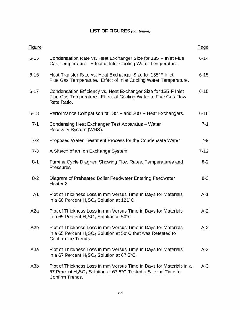
LIST OF FIGURES (continued)
Figure Page 6-15 Condensation Rate vs. Heat Exchanger Size for 135°F Inlet Flue 6-14 Gas Temperature. Effect of Inlet Cooling Water Temperature. 6-16 Heat Transfer Rate vs. Heat Exchanger Size for 135°F Inlet 6-15 Flue Gas Temperature. Effect of Inlet Cooling Water Temperature. 6-17 Condensation Efficiency vs. Heat Exchanger Size for 135°F Inlet 6-15 Flue Gas Temperature. Effect of Cooling Water to Flue Gas Flow Rate Ratio. 6-18 Performance Comparison of 135°F and 300°F Heat Exchangers. 6-16 7-1 Condensing Heat Exchanger Test Apparatus – Water 7-1 Recovery System (WRS). 7-2 Proposed Water Treatment Process for the Condensate Water 7-9 7-3 A Sketch of an Ion Exchange System 7-12 8-1 Turbine Cycle Diagram Showing Flow Rates, Temperatures and 8-2 Pressures 8-2 Diagram of Preheated Boiler Feedwater Entering Feedwater 8-3 Heater 3 A1 Plot of Thickness Loss in mm Versus Time in Days for Materials A-1 in a 60 Percent H2SO4 Solution at 121°C. A2a Plot of Thickness Loss in mm Versus Time in Days for Materials A-2 in a 65 Percent H2SO4 Solution at 50°C. A2b Plot of Thickness Loss in mm Versus Time in Days for Materials A-2 in a 65 Percent H2SO4 Solution at 50°C that was Retested to Confirm the Trends. A3a Plot of Thickness Loss in mm Versus Time in Days for Materials A-3 in a 67 Percent H2SO4 Solution at 67.5°C. A3b Plot of Thickness Loss in mm Versus Time in Days for Materials in a A-3 67 Percent H2SO4 Solution at 67.5°C Tested a Second Time to Confirm Trends.
xvii
LIST OF FIGURES (continued)
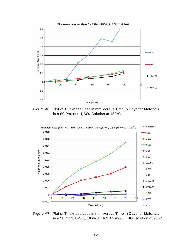
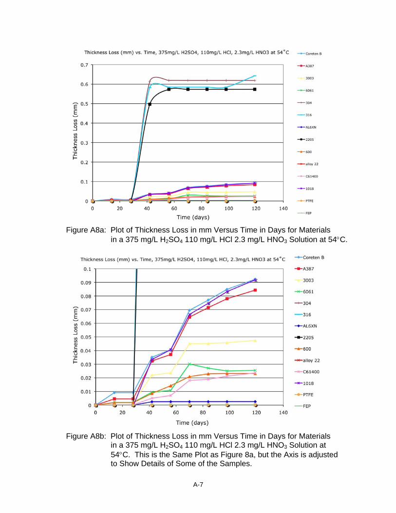
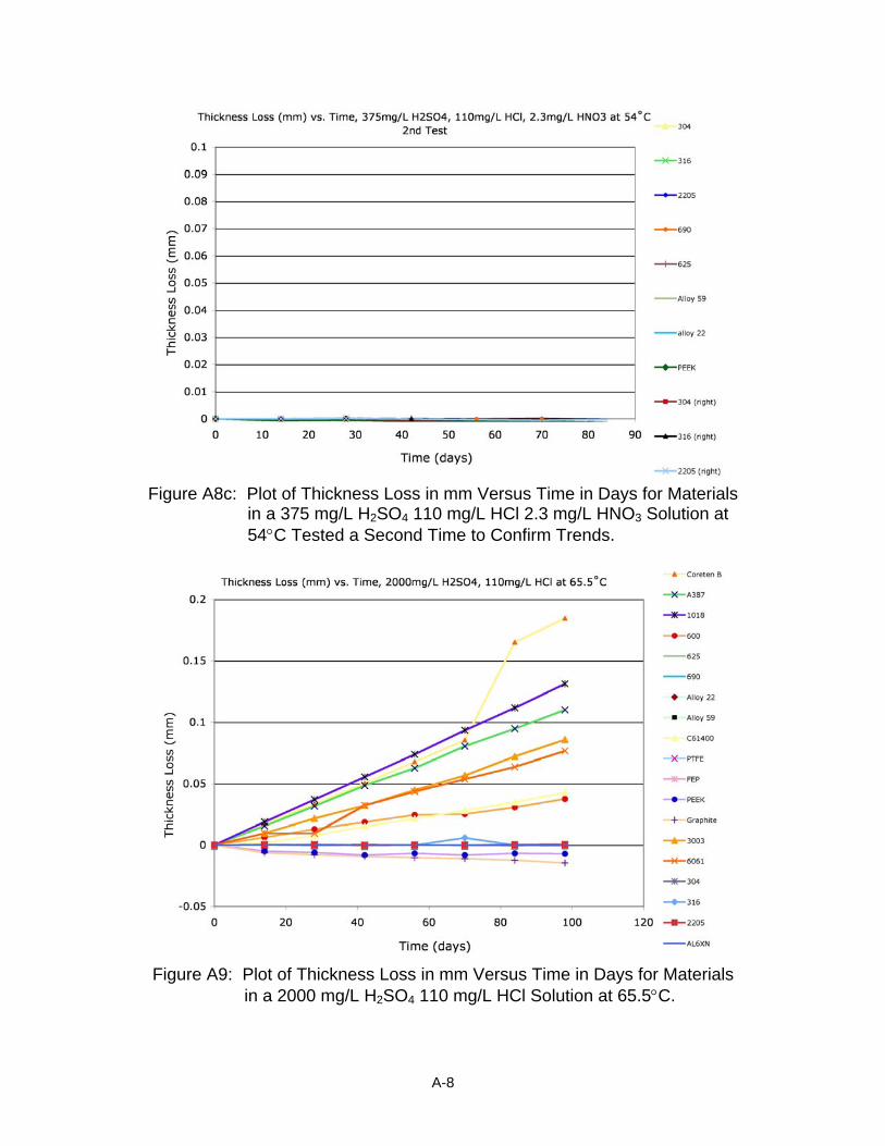
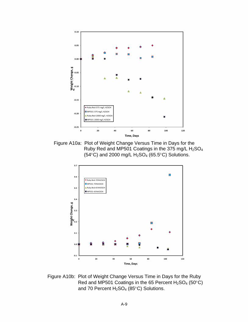
Figure Page A4a Plot of Thickness Loss in mm Versus Time in Days for Materials A-4 in a 70 Percent H2SO4 Solution at 85°C. A4b Plot of Thickness Loss in mm Versus Time in Days for Materials A-4 in a 70 Percent H2SO4 Solution at 85°C Tested for a Second Time to Confirm Trends. A5a Plot of Thickness Loss in mm Versus Time in Days for Materials A-5 in a 74 Percent H2SO4 Solution at 115°C. A5b Plot of Thickness Loss in mm Versus Time in Days for Materials A-5 in a 74 Percent H2SO4 Solution at 115°C Tested a Second Time to Confirm Trends. A6 Plot of Thickness Loss in mm Versus Time in Days for Materials A-6 in a 80 Percent H2SO4 Solution at 150°C. A7 Plot of Thickness Loss in mm Versus Time in Days for Materials A-6 in a 50 mg/L H2SO4 10 mg/L HCl 0.5 mg/L HNO3 solution at 21°C. A8a Plot of Thickness Loss in mm Versus Time in Days for Materials A-7 in a 375 mg/L H2SO4 110 mg/L HCl 2.3 mg/L HNO3 Solution at 54°C. A8b Plot of Thickness Loss in mm Versus Time in Days for Materials A-7 in a 375 mg/L H2SO4 110 mg/L HCl 2.3 mg/L HNO3 Solution at 54°C. This is the Same Plot as Figure 8a, but the Axis is adjusted to Show Details of Some of the Samples. A8c Plot of Thickness Loss in mm Versus Time in Days for Materials A-8 in a 375 mg/L H2SO4 110 mg/L HCl 2.3 mg/L HNO3 Solution at 54°C Tested a Second Time to Confirm Trends. A9 Plot of Thickness Loss in mm Versus Time in Days for Materials A-8 in a 2000 mg/L H2SO4 110 mg/L HCl Solution at 65.5°C. A10a Plot of Weight Change Versus Time in Days for the Ruby Red A-9 and MP501 Coatings in the 375 mg/L H2SO4 (54°C) and 2000 mg/L H2SO4 (65.5°C) Solutions. A10b Plot of Weight Change Versus Time in Days for the Ruby Red and A-9 MP501 Coatings in the 65 Percent H2SO4 (50°C) and 70 Percent H2SO4 (85°C) Solutions.
xviii
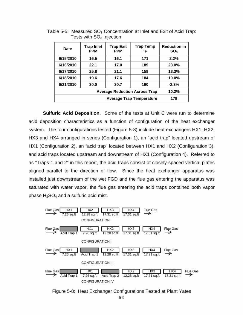
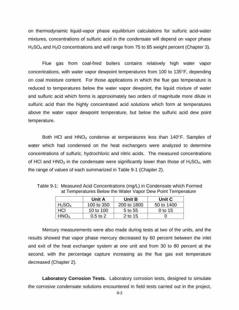
EXECUTIVE SUMMARY Coal-fired power plants have traditionally operated with stack temperatures in the 300°F range to minimize acid corrosion and provide a buoyancy force to assist in the transport of flue gas up the stack. However, as an alternative, there would be benefits to cooling the flue gas to temperatures below the water vapor dew point. The condensed water vapor would provide a source of water for use in power plant cooling; recovered latent and sensible heat could be used to reduce unit heat rate; the reduced flue gas temperature would promote increased mercury removal; and the availability of low-temperature flue gas with reduced acid and water vapor content would reduce the costs of capturing CO2 in back end amine and ammonia CO2 scrubbers. This report, which is the final technical report for DOE project DE-NT0005648, describes the continued development of condensing heat exchanger technology for coal-fired boilers. In particular, the report describes results of slip stream tests performed at coal-fired power plants, theoretical predictions for acid concentrations in liquid deposits at surface temperatures above the water vapor dewpoint temperature, laboratory corrosion data on candidate tube materials, data on the effectiveness of acid traps in reducing sulfuric acid concentrations in heat exchanger tube bundles, designs of full scale heat exchangers and installed capital costs, condensed water treatment needs and costs, and results of cost-benefit studies of condensing heat exchangers. Power Plant Slip Stream Tests. An expanded data base on water and acid condensation characteristics of boiler flue gas with water-cooled condensing heat exchangers was generated from slip stream tests at coal-fired power plants. The units included one which fires high sulfur bituminous coal and has a wet FGD scrubber and two which are unscrubbed and fire high-moisture low rank coals. In the case of the two unscrubbed units, the flue gas slip streams were obtained from flue gas ducts downstream of the ESP’s, while the flue gas slip stream from the third boiler was taken just downstream of the wet FGD. The results show strong dependence of total heat transfer and water vapor capture efficiency on flow rate ratio of cooling water to flue gas and inlet cooling water temperature. If cold boiler feedwater is used as the cooling fluid, the flow rate ratio of cooling water to flue gas will be approximately 0.5 and water vapor capture efficiencies will be limited to approximately 20 percent. For applications in which flow rates of cooling water greater than the flow rate of cold boiler feedwater are available, water vapor capture efficiencies significantly greater than 20 percent will be possible. As boiler flue gas is reduced in temperature below the sulfuric acid dew point, the acid first condenses as a highly concentrated solution of sulfuric acid and water. Based on thermodynamic liquid-vapor phase equilibrium calculations for sulfuric acid-water mixtures, concentrations of sulfuric acid in the condensate will depend on vapor phase H2SO4 and H2O concentrations and will range from 75 to 85 weight percent. Depending on coal moisture content, flue gas from coal-fired boilers has water vapor dewpoint temperatures from 100 to 135°F. For those applications in which the
xix
flue gas temperature is reduced to temperatures below the water vapor dewpoint, the liquid mixture of water and sulfuric acid which forms is several orders of magnitude more dilute in sulfuric acid than the highly concentrated acid solutions which form at temperatures above the water vapor dewpoint temperature, but below the sulfuric acid dew point temperature. Both HCl and HNO3 condense at temperatures less than 140°F and their concentrations in low temperature aqueous condensate are significantly lower than those of H2SO4. Flue gas mercury measurements showed that vapor phase mercury decreased by 60 percent between the inlet and exit of the heat exchanger system at one unit and from 30 to 80 percent at the second, with the percentage capture increasing as the flue gas exit temperature decreased. Laboratory Corrosion Tests. Laboratory corrosion tests, designed to simulate the corrosive condensate solutions encountered in the slip stream field tests, were conducted to identify materials which would have adequate service life. The tests were performed in aqueous solutions containing sulfuric acid at concentration levels representative of both dilute and high acid concentration conditions. All materials tested except carbon steel exhibited acceptable corrosion rates in dilute acid solutions. Of the remaining alloys, 304 stainless steel was found to be the preferred choice due to relatively low cost, ease of fabrication, and negligible corrosion rates over the entire range of test conditions. Alloys 22 and 690 along with two Teflon materials (FEP and PTFE) showed the best performance at high acid concentration conditions. Of these, Alloy 22 is preferred for service in high acid concentrations due to its low corrosion rate, high yield strength and thermal conductivity, and ability to be readily fabricated. Effectiveness of Acid Traps. Tests were performed to assess the potential of reducing the flue gas sulfuric acid concentration entering the heat exchangers through use of additional surface area in the inlet region to capture a portion of the inlet H2SO4. The concept involves use of a section of inlet duct filled with closely spaced vertical flat plates aligned parallel to the flow direction (referred to as “acid traps” in this report). The test results show that at temperatures above the water vapor dewpoint, the acid traps reduced the vapor phase acid concentrations entering the heat exchangers just downstream of the traps by 10.2 to 13.7 percent. At temperatures at or below the water vapor dew point, the presence of an acid trap reduced the sulfuric acid flux on the heat exchanger positioned just downstream of the trap by 33 to 42 percent. Design of Full-Scale Heat Exchangers. Heat exchanger design calculations were made to estimate how much flue gas moisture it would be possible to recover from boiler flue gas, the size and cost of the heat exchangers, and flue gas and cooling water pressure drops. The laboratory corrosion test data showed that at locations in the flue gas upstream of the water vapor dewpoint, the choice of tube material is between Teflon and Alloy 22. The design analyses showed that in order to transfer the same amount of heat, the Teflon heat exchanger would need to have approximately three
xx
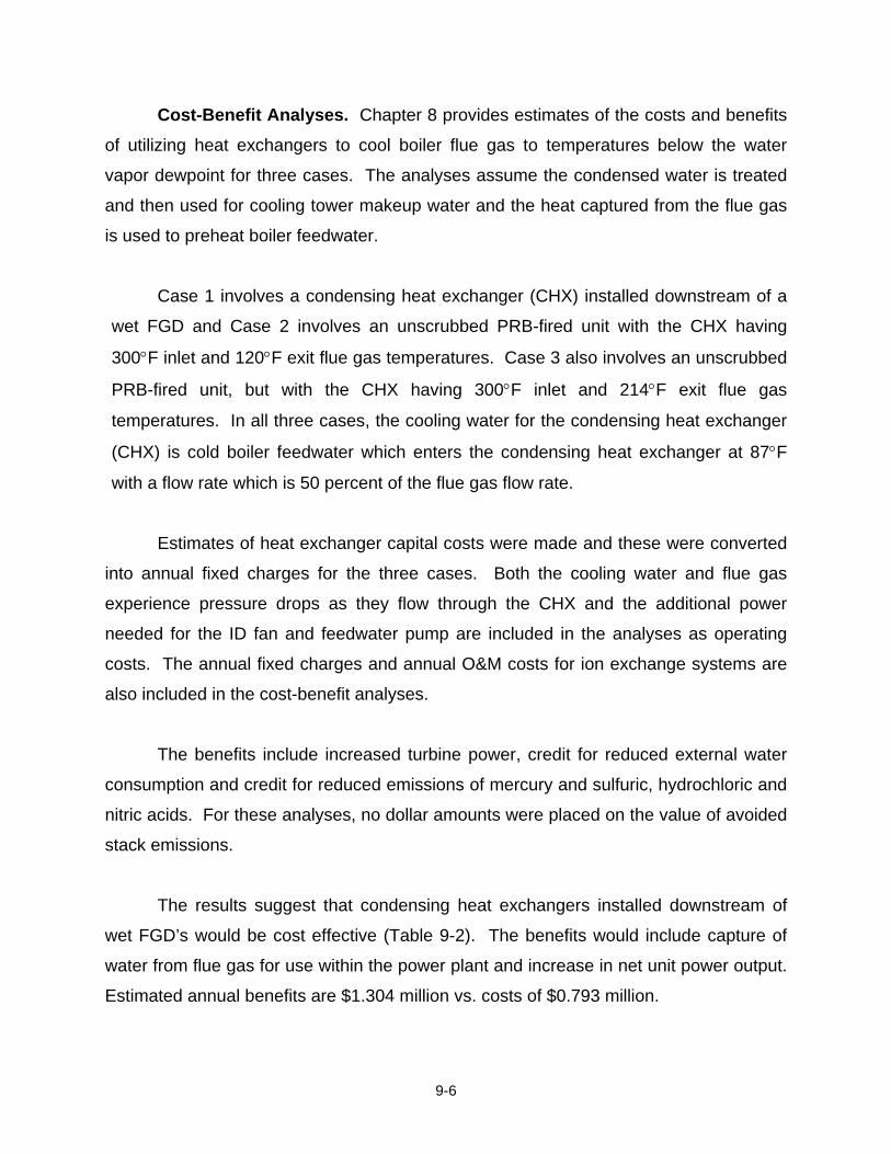
times the surface area of an Alloy 22 heat exchanger, and this would also result in larger pump and fan power requirements than would be needed for the Alloy 22 heat exchanger. As a consequence, the total annual costs for a Teflon heat exchanger would be greater than for a heat exchanger fabricated from Alloy 22. Because of its corrosion resistance in aqueous solutions with low acid concentrations, relatively low cost and high tensile strength and thermal conductivity, 304 SS is the preferred choice for heat exchanger tubing at temperatures below the water vapor dew point. There will be separate applications for condensing heat exchangers, depending on coal type. A boiler firing a Powder River Basin coal may not need a wet SO2 scrubber, and in this case, the flue gas temperature at the inlet of the condensing heat exchanger will be in the 300°F range with inlet water vapor concentrations of approximately 12 volume percent. For those applications in which a wet FGD is needed for SO2 control (bituminous coals and some lignites typically require wet FGD’s), the flue gas entering the condensing heat exchanger will be saturated with water vapor and have a temperature ranging from 125 to 135°F, with the temperature depending on coal moisture content. Treatment of Condensed Water. Ion exchange and reverse osmosis technologies were evaluated for treatment of condensed water from flue gas water recovery heat exchangers, with the goal of using the recovered water as cooling tower makeup water. Comparisons of the chemical composition of condensed water with cooling tower water, makeup water, and river water samples reveal that they are comparable except for nitrate, sulfate, iron and pH level. An ion exchange system is recommended for this application, and cost analysis of the ion exchange system revealed that the cost of water treatment would be approximately $0.001/gallon. Cost-Benefit Analyses. Estimates of the costs and benefits of utilizing heat exchangers to cool boiler flue gas to temperatures below the water vapor dewpoint were made for three cases. The analyses assume the condensed water is treated and the heat captured from the flue gas is used to preheat boiler feedwater. Case 1 involves a heat exchanger installed downstream of a wet FGD and Case 2 involves an unscrubbed PRB-fired unit with the heat exchanger having 300°F inlet and 120°F exit flue gas temperatures. Case 3 also involves an unscrubbed PRB-fired unit, but with the heat exchanger having 300°F inlet and 214°F exit flue gas temperatures. In all three cases, the cooling water for the condensing heat exchanger is cold boiler feedwater which enters the heat exchanger at 87°F with a flow rate which is 50 percent of the flue gas flow rate.
Estimates of heat exchanger capital costs were made and these were converted into annual fixed charges for the three cases. Both the cooling water and flue gas experience pressure drops as they flow through the heat exchanger and the additional power needed for the ID fan and feedwater pump are included in the analyses as
xxi
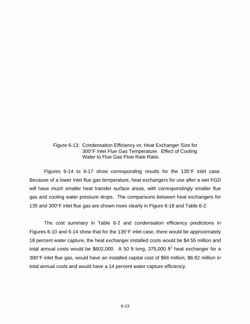
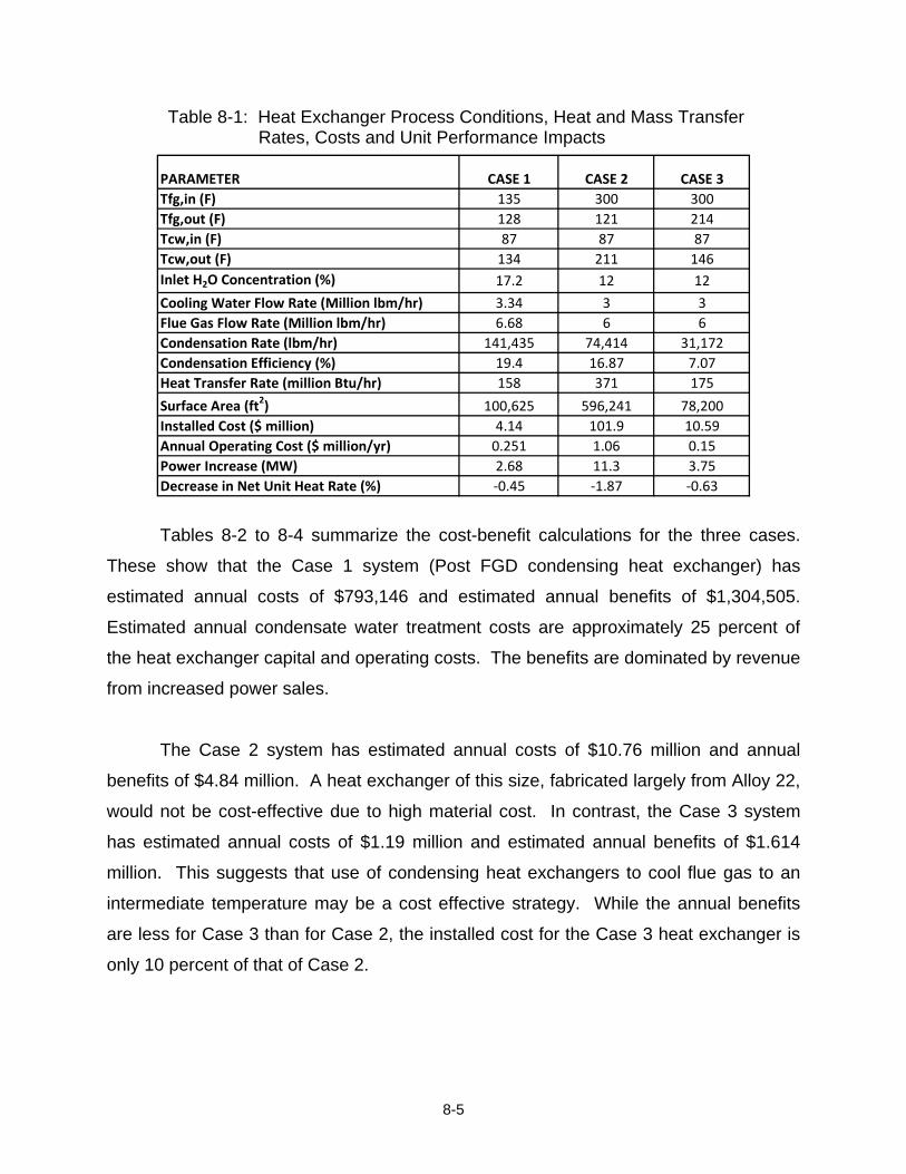
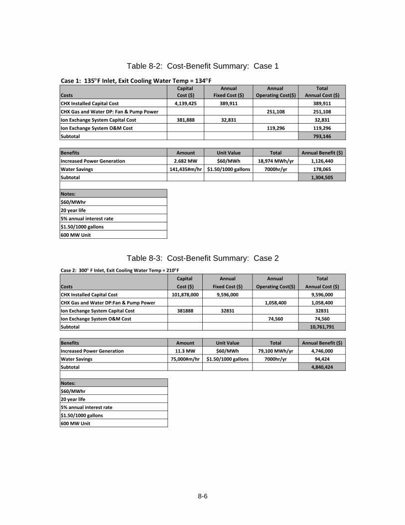
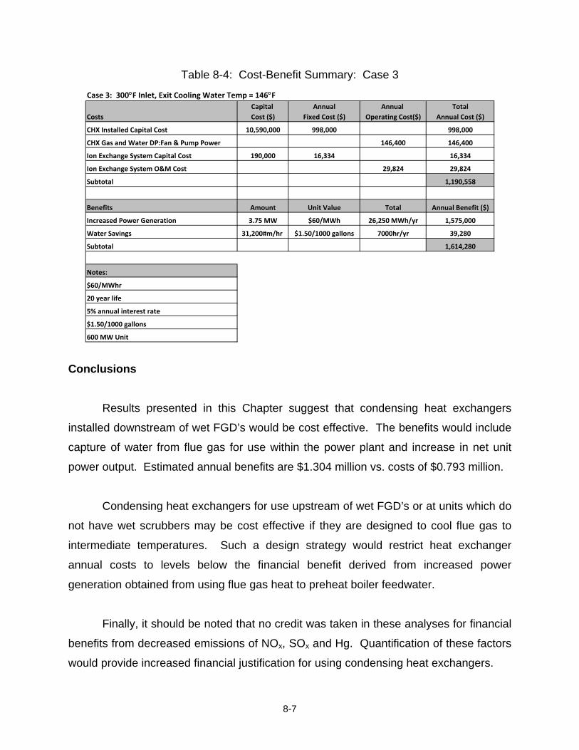
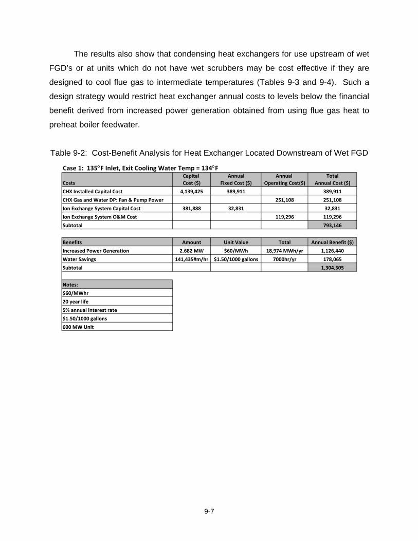
operating costs. The annual fixed charges and annual O&M costs for ion exchange systems are also included in the cost-benefit analyses. The benefits include increased turbine power, credit for reduced external water consumption and credit for reduced emissions of mercury and sulfuric, hydrochloric and nitric acids. For these analyses, no dollar amounts were placed on the value of avoided stack emissions. The results suggest that condensing heat exchangers installed downstream of wet FGD’s would be cost effective. The benefits would include capture of water from flue gas for use within the power plant and increase in net unit power output. Estimated annual benefits are $1.304 million vs. costs of $0.793 million. The results also show that condensing heat exchangers for use upstream of wet FGD’s or at units which do not have wet scrubbers may be cost effective if they are designed to cool flue gas to intermediate temperatures. Such a design strategy would restrict heat exchanger annual costs to levels below the financial benefit derived from increased power generation obtained from using flue gas heat to preheat boiler feedwater.
1-1
CHAPTER 1
Introduction
As the U.S. population grows and demand for electricity and water increase,
power plants located in some parts of the country will find it increasingly difficult to
obtain the large quantities of water needed to maintain operations. Most of the water
used in a thermoelectric power plant is used for cooling, and DOE has been focusing on
possible techniques to reduce the amount of fresh water needed for cooling. DOE has
also been placing emphasis on recovery of usable water from sources not generally
considered, such as mine water, water produced from oil and gas extraction, and water
contained in boiler flue gas.
The moisture in boiler flue gas comes from three sources … fuel moisture, water
vapor formed from the oxidation of fuel hydrogen, and water vapor carried into the boiler
with the combustion air. The amounts of H2O vapor in flue gas depend heavily on coal
rank. Calculation of typical coal flow rates and flue gas moisture flow rates for 600 MW
pulverized coal power plants show that flue gas moisture flow rates range from
approximately 225,000 to more than 650,000 lbs/hr. In contrast, typical cooling tower
water evaporation rates for a 600 MW unit are 2.1 million lbs/hr. Thus, coal-fired power
plants, equipped with a means of extracting all the flue gas moisture and using it for
cooling tower makeup, would be able to supply from 10 percent to 33 percent of the
makeup water by this approach (Table 1-1).
Table 1-1: Estimated Fractions of Cooling Tower Makeup Water Provided
by Condensing Heat Exchangers, Assuming 100 Percent Water Vapor Capture
Case Inlet Flue Gas Moisture Fraction (Volume Percentage)
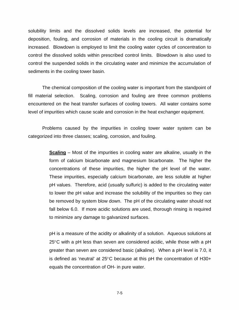
Many coal-fired power plants operate with stack temperatures in the 300°F range
to minimize fouling and corrosion problems due to sulfuric acid condensation and to
provide a buoyancy force to assist in the transport of flue gas up the stack. With SO3
concentrations up to 35 ppm, sulfuric acid begins condensing at temperatures from 250
to 310°F (Figure 1-1), and with flue gas water vapor volume concentrations typically
from 6 to 17.5 volume percent, depending on coal rank, the water vapor dewpoint is
usually in the 100 to 135°F range (Figure 1-2). Other acids (hydrochloric, and nitric, for
example) condense in the same temperature range as H2O (Figure 1-3).
There would be significant benefits to cooling the flue gas to temperatures below
the water vapor and acid dew points, provided the acid corrosion problems can be
overcome in a cost-effective way. With stack temperatures below the water vapor dew
point, condensed water vapor would provide a source of water for use in power plant
cooling; recovered latent and sensible heat from the flue gas could be used to reduce
unit heat rate and thereby reduce CO2 emissions; condensation of acid in a controlled
manner would reduce the flue gas acid content and provide environmental, operational
and maintenance benefits; the reduced flue gas temperature would promote increased
mercury removal; and the availability of low temperature flue gas with reduced acid and
water vapor content would reduce the costs of capturing CO2 at the back end of the
boiler.
Figure 1-1: Sulfuric Acid Dew Point Temperature vs. Acid Concentration (Refs. 1 to 4)
1-3
HCl and HNO3 Dew Points
0.1
1.0
10.0
100.0
1000.0
0 20 40 60 80 100 120 140 160
Dew Point Temperature (°F)
ppm
HCl 5% Vol% H20
HCl 10% Vol% H20
HCl 15% Vol% H20
HNO3 5% Vol% H20
HNO3 10% Vol% H20
HNO3 15% Vol% H20
H2O Dew Point
0%
2%
4%
6%
8%
10%
12%
14%
16%
40 60 80 100 120 140 160
Dew Point Temperature (°F)
Volu
met
ric P
erce
ntag
e
Figure 1-2: Water Vapor Dew Point vs. Volumetric Concentration (Ref 5)
Figure 1-3: Dew Point Temperatures of Hydrochloric and Nitric Acids (Ref 6 and 7) Under DOE project DE-FC26-06NT42727, “Recovery of Water from Boiler Flue Gas,” Lehigh University investigated the heat transfer and water vapor and acid condensation characteristics of condensing heat exchangers (Ref. 8). The present
1-4
report, which is the final technical report for DOE project DE-NT0005648, describes the continued development of condensing heat exchanger technology for coal-fired boilers. In particular, the report describes:
• An expanded data base on water and acid condensation characteristics of condensing heat exchangers in coal-fired units. This data base was generated by performing slip stream tests at a power plant with high sulfur bituminous coal and a wet FGD scrubber and at a power plant firing high-moisture, low rank coals (Chapter 2).
• Data on typical concentrations of HCl, HNO3 and H2SO4 in low temperature condensed flue gas moisture (Chapter 2).
• Theoretical predictions for sulfuric acid concentrations on tube surfaces at temperatures above the water vapor dewpoint temperature, and below the sulfuric acid dew point temperature (Chapter 3).
• Data on corrosion rates of candidate heat exchanger tube materials for the different regions of the heat exchanger system as functions of acid concentration and temperature (Chapter 4).
• Data on effectiveness of acid traps in reducing sulfuric acid concentrations in a heat exchanger tube bundle. Mercury capture efficiencies as functions of process conditions in power plant field tests (Chapter 5).
• Condensing heat exchanger designs and installed capital costs for full scale applications, both for installation immediately downstream of an ESP or baghouse and for installation downstream of a wet SO2 scrubber (Chapter 6).
• Condensed flue gas water treatment needs and costs (Chapter 7). • Results of cost-benefit studies of condensing heat exchangers (Chapter 8).
References
1. Rylands, J. R., and J. R. Jenkinson, “The Acid Dewpoint,” Journal of the Institute of Fuel, Vol. 27, 1954, pp. 299-309.
2. Gmitro, J. I., and T. Vermeulen, “Vapor-Liquid Equilibria for Aqueous Sulfuric Acid,” AIChE Journal, Vol. 10, 1964, pp. 740-746.
3. Halstead, W. D., “The Sulfuric Acid Dewpoint in Power Station Flue Gases,” Journal of the Institute of Energy, Vol. 53, September 1980, pp. 142-145.
1-5
4. Banchero, J. T., and F. H. Verhoff, “Evaluation and Interpretation of the Vapour Pressure Data for Sulfuric Acid Aqueous Solutions with Applications to Flue Gas Dewpoints,” Journal of the Institute of Fuel, Vol. 48, 1975, pp. 76-80.
5. Thermodynamic Properties of Steam, J. Keenan and F. Keyes. John Wiley. 1936.
6. Verhoff, F. H. and J. T. Banchero, “Predicting Dew Points of Flue Gases,” Chem. Eng. Progress, 1974, Vol. 70, pp. 71-72.
7. Yen Hsiung Kiang, “Predicting Dewpoints of Acid Gases,” Chemical Engineering, February 9, 1981, p. 127.
8. Levy, E. et al, “Recovery of Water from Boiler Flue Gas,” Final Technical Report for DOE Project DE-FC26-06NT42727, December, 2008.
2-1
CHAPTER 2
POWER PLANT SLIP STREAM TESTS OF HEAT EXCHANGERS Introduction
This chapter describes the results of slipstream heat transfer and water vapor
condensation tests performed at three coal-fired power plants. In addition, data are
presented on rates of acid condensation on the heat exchangers and on the effects of
the heat exchangers on flue gas mercury content.
Flue Gas and Cooling Water Conditions
The heat exchanger applications described in this Chapter are for two distinct
flue gas process conditions. For a coal-fired unit without a wet FGD, the heat
exchanger system would be located downstream of the ESP or baghouse and would
cool the flue gas to temperatures below the water vapor dew point temperature. Inlet
flue gas moisture concentration will depend on coal type, and will range from
approximately 6 to 8 volumetric percent for bituminous coal to values of 12 to13 percent
for North American lignites. In the case of a unit with a wet FGD, the possibility exists
for heat exchangers to be located both upstream and downstream of the FGD. Flue
gas exiting the FGD is typically in the 125°F to 140°F temperature range and is
saturated with water vapor. A heat exchanger located upstream of the FGD would
capture sensible heat and a heat exchanger located downstream of the FGD would both
cool the flue gas (sensible heat transfer) and condense water vapor from the flue gas
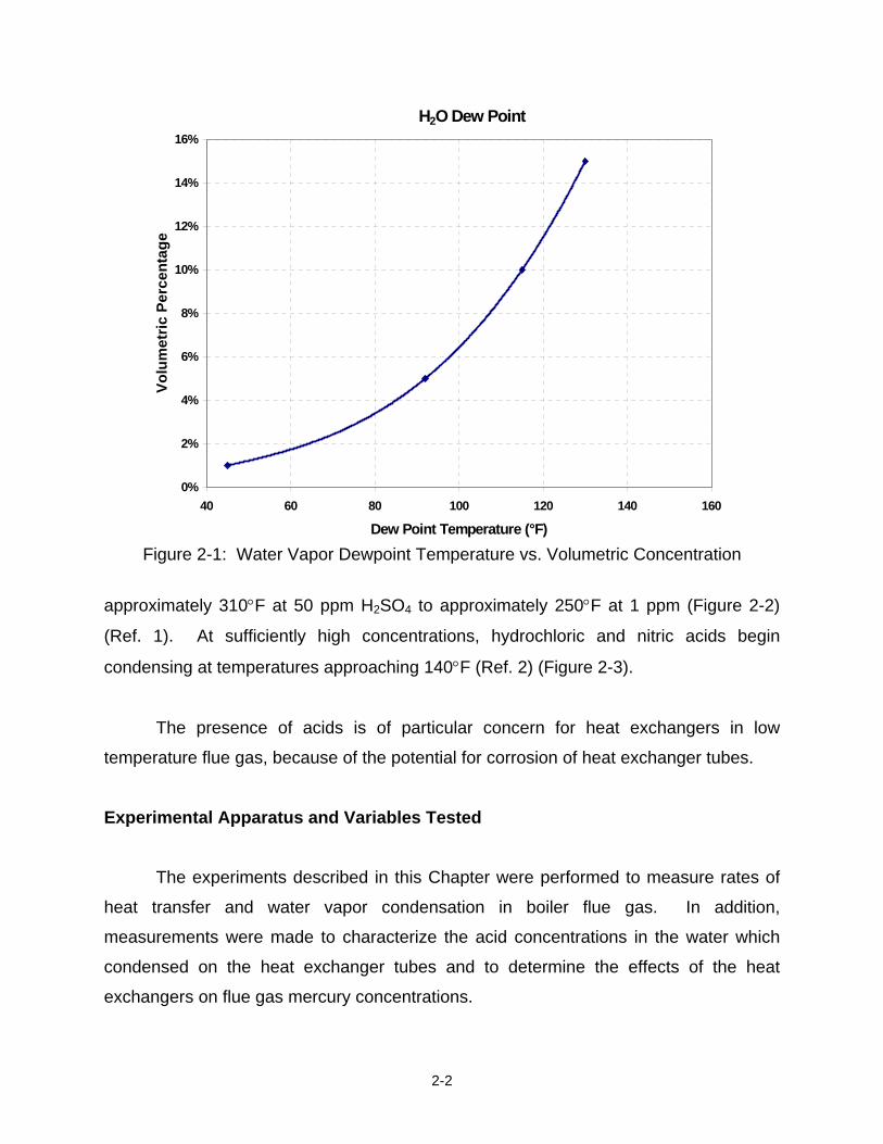
(latent heat transfer). Figure 2-1 shows the relationship between water vapor dewpoint
temperature and volume concentration for flue gas at atmospheric pressure.
In addition to water vapor, flue gas from coal contains sulfuric, hydrochloric and
nitric acids. Typical flue gas sulfuric acid concentrations range from a few ppm to
values in excess of 40 ppm. Sulfuric acid dew point temperature depends on both
sulfuric acid and water vapor concentrations, with dew point temperatures ranging from
2-2
H2O Dew Point
0%
2%
4%
6%
8%
10%
12%
14%
16%
40 60 80 100 120 140 160
Dew Point Temperature (°F)
Volu
met
ric P
erce
ntag
e
Figure 2-1: Water Vapor Dewpoint Temperature vs. Volumetric Concentration
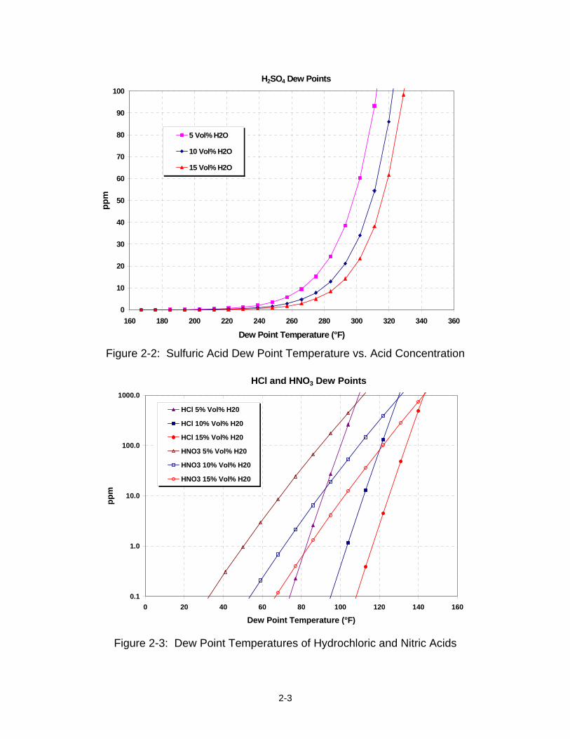
approximately 310°F at 50 ppm H2SO4 to approximately 250°F at 1 ppm (Figure 2-2)
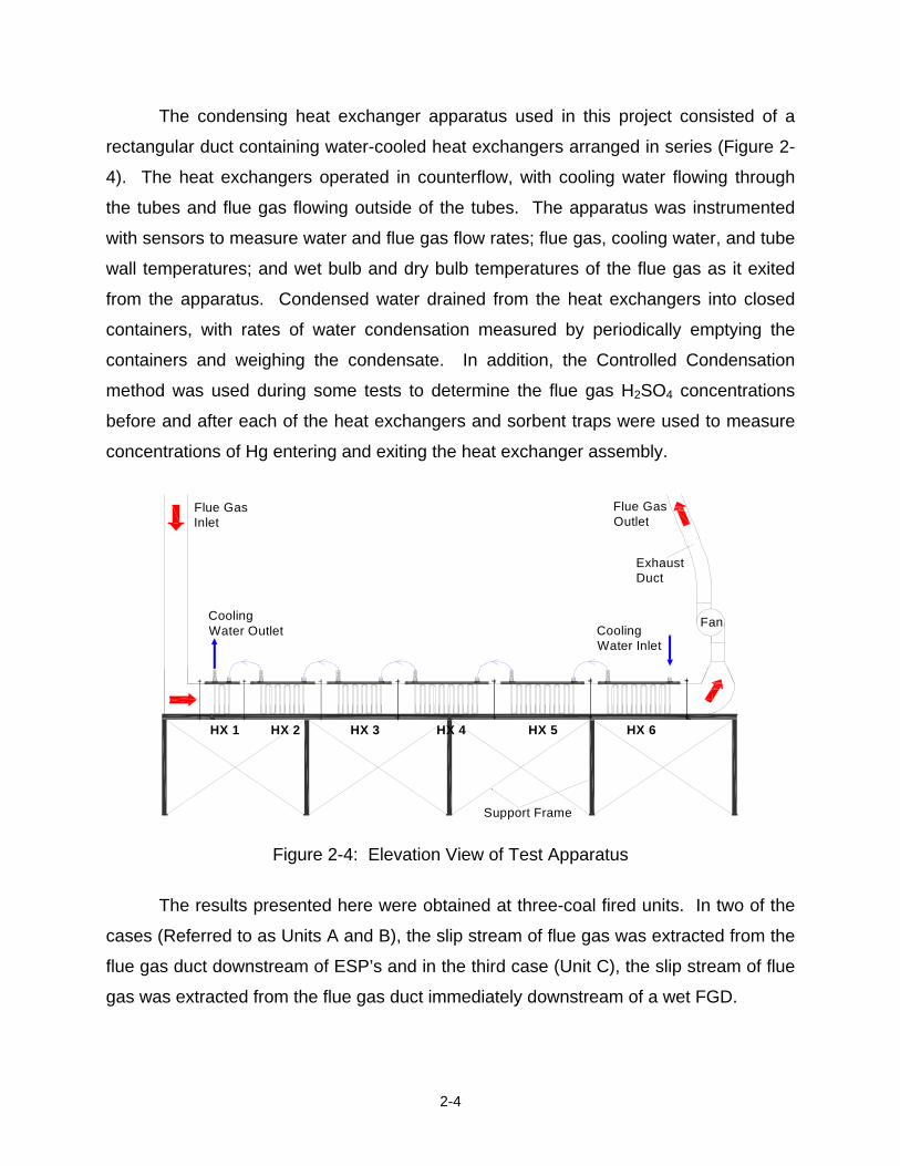
(Ref. 1). At sufficiently high concentrations, hydrochloric and nitric acids begin
condensing at temperatures approaching 140°F (Ref. 2) (Figure 2-3).
The presence of acids is of particular concern for heat exchangers in low
temperature flue gas, because of the potential for corrosion of heat exchanger tubes.
Experimental Apparatus and Variables Tested The experiments described in this Chapter were performed to measure rates of
heat transfer and water vapor condensation in boiler flue gas. In addition,
measurements were made to characterize the acid concentrations in the water which
condensed on the heat exchanger tubes and to determine the effects of the heat
exchangers on flue gas mercury concentrations.
2-3
H2SO4 Dew Points
0
10
20
30
40
50
60
70
80
90
100
160 180 200 220 240 260 280 300 320 340 360
Dew Point Temperature (°F)
ppm
5 Vol% H2O
10 Vol% H2O
15 Vol% H2O
HCl and HNO3 Dew Points
0.1
1.0
10.0
100.0
1000.0
0 20 40 60 80 100 120 140 160
Dew Point Temperature (°F)
ppm
HCl 5% Vol% H20
HCl 10% Vol% H20
HCl 15% Vol% H20
HNO3 5% Vol% H20
HNO3 10% Vol% H20
HNO3 15% Vol% H20
Figure 2-2: Sulfuric Acid Dew Point Temperature vs. Acid Concentration
Figure 2-3: Dew Point Temperatures of Hydrochloric and Nitric Acids
2-4
CoolingWater Outlet
Fan
Flue GasOutlet
Exhaust Duct
Flue Gas Inlet
HX 1 HX 2 HX 3 HX 4
Support Frame
HX 5 HX 6
CoolingWater Inlet
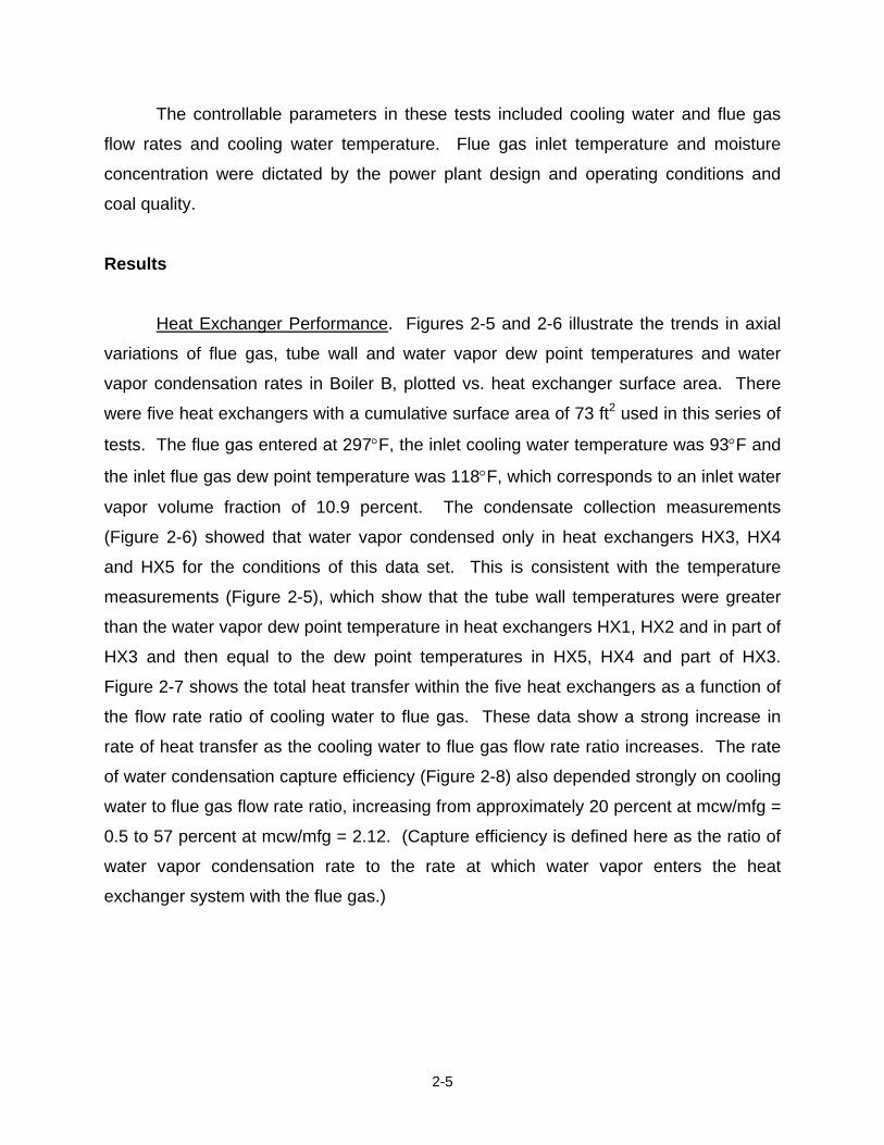
The condensing heat exchanger apparatus used in this project consisted of a
rectangular duct containing water-cooled heat exchangers arranged in series (Figure 2-
4). The heat exchangers operated in counterflow, with cooling water flowing through
the tubes and flue gas flowing outside of the tubes. The apparatus was instrumented
with sensors to measure water and flue gas flow rates; flue gas, cooling water, and tube
wall temperatures; and wet bulb and dry bulb temperatures of the flue gas as it exited
from the apparatus. Condensed water drained from the heat exchangers into closed
containers, with rates of water condensation measured by periodically emptying the
containers and weighing the condensate. In addition, the Controlled Condensation
method was used during some tests to determine the flue gas H2SO4 concentrations
before and after each of the heat exchangers and sorbent traps were used to measure
concentrations of Hg entering and exiting the heat exchanger assembly.
Figure 2-4: Elevation View of Test Apparatus
The results presented here were obtained at three-coal fired units. In two of the
cases (Referred to as Units A and B), the slip stream of flue gas was extracted from the
flue gas duct downstream of ESP’s and in the third case (Unit C), the slip stream of flue
gas was extracted from the flue gas duct immediately downstream of a wet FGD.
2-5
The controllable parameters in these tests included cooling water and flue gas
flow rates and cooling water temperature. Flue gas inlet temperature and moisture
concentration were dictated by the power plant design and operating conditions and
coal quality.
Results
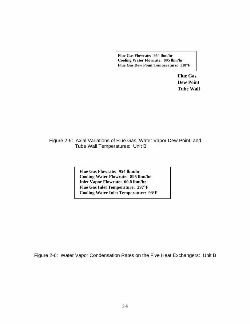
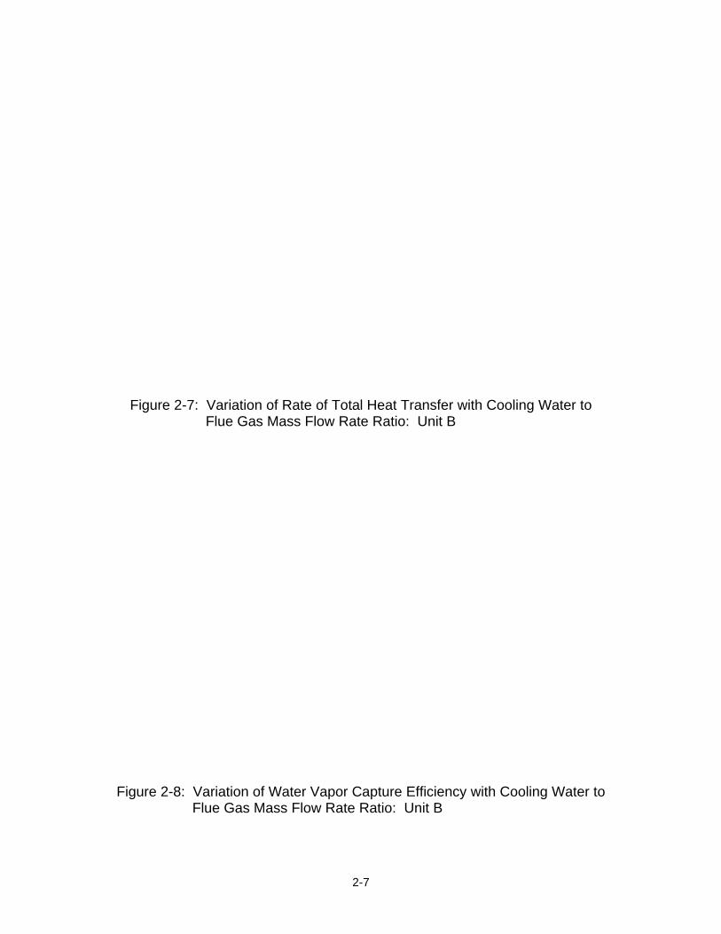
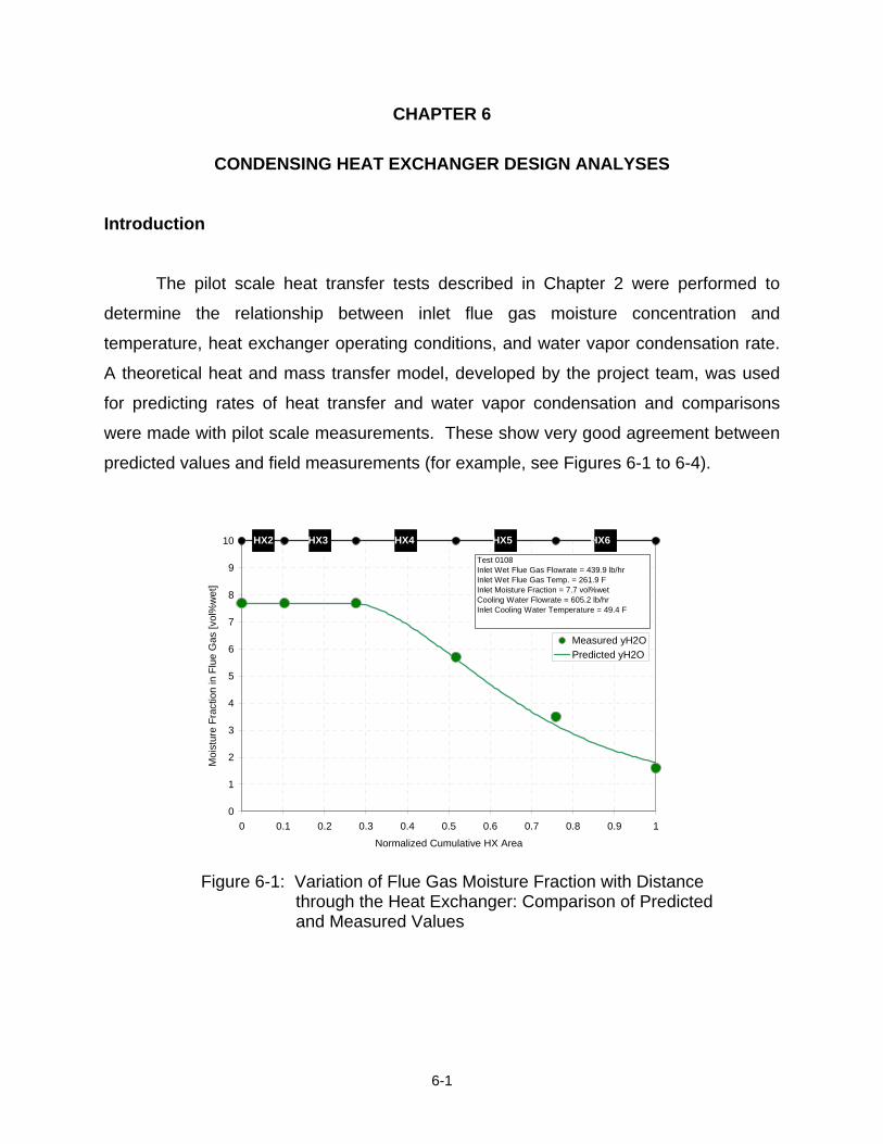
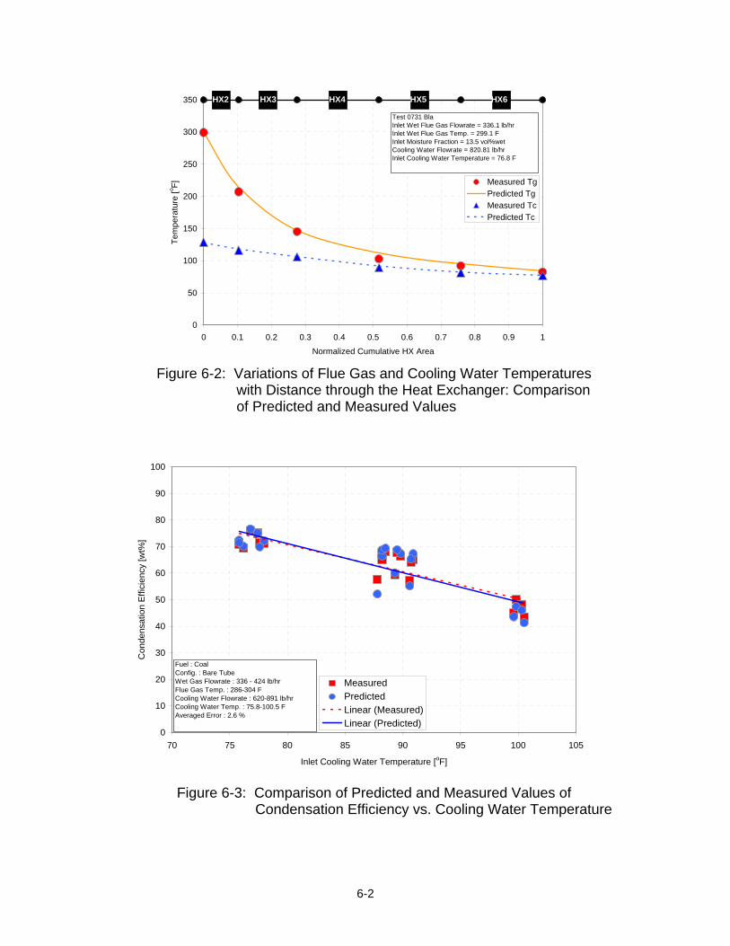
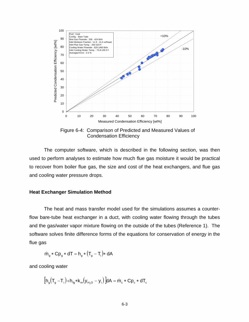
Heat Exchanger Performance. Figures 2-5 and 2-6 illustrate the trends in axial
variations of flue gas, tube wall and water vapor dew point temperatures and water
vapor condensation rates in Boiler B, plotted vs. heat exchanger surface area. There
were five heat exchangers with a cumulative surface area of 73 ft2 used in this series of
tests. The flue gas entered at 297°F, the inlet cooling water temperature was 93°F and
the inlet flue gas dew point temperature was 118°F, which corresponds to an inlet water
vapor volume fraction of 10.9 percent. The condensate collection measurements
(Figure 2-6) showed that water vapor condensed only in heat exchangers HX3, HX4
and HX5 for the conditions of this data set. This is consistent with the temperature
measurements (Figure 2-5), which show that the tube wall temperatures were greater
than the water vapor dew point temperature in heat exchangers HX1, HX2 and in part of
HX3 and then equal to the dew point temperatures in HX5, HX4 and part of HX3.
Figure 2-7 shows the total heat transfer within the five heat exchangers as a function of
the flow rate ratio of cooling water to flue gas. These data show a strong increase in
rate of heat transfer as the cooling water to flue gas flow rate ratio increases. The rate
of water condensation capture efficiency (Figure 2-8) also depended strongly on cooling
water to flue gas flow rate ratio, increasing from approximately 20 percent at mcw/mfg =
0.5 to 57 percent at mcw/mfg = 2.12. (Capture efficiency is defined here as the ratio of
water vapor condensation rate to the rate at which water vapor enters the heat
exchanger system with the flue gas.)
2-6
Flue Gas Flowrate: 954 lbm/hr Cooling Water Flowrate: 895 lbm/hr Inlet Vapor Flowrate: 60.0 lbm/hr Flue Gas Inlet Temperature: 297°F Cooling Water Inlet Temperature: 93°F
Figure 2-5: Axial Variations of Flue Gas, Water Vapor Dew Point, and Tube Wall Temperatures: Unit B
Figure 2-6: Water Vapor Condensation Rates on the Five Heat Exchangers: Unit B
Flue Gas Flowrate: 954 lbm/hr Cooling Water Flowrate: 895 lbm/hr Flue Gas Dew Point Temperature: 118°F
Flue Gas Dew Point Tube Wall
2-7
Figure 2-7: Variation of Rate of Total Heat Transfer with Cooling Water to Flue Gas Mass Flow Rate Ratio: Unit B
Figure 2-8: Variation of Water Vapor Capture Efficiency with Cooling Water to Flue Gas Mass Flow Rate Ratio: Unit B
2-8
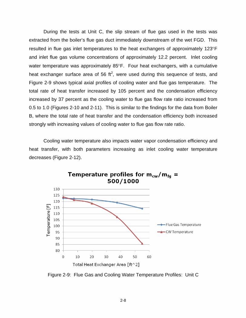
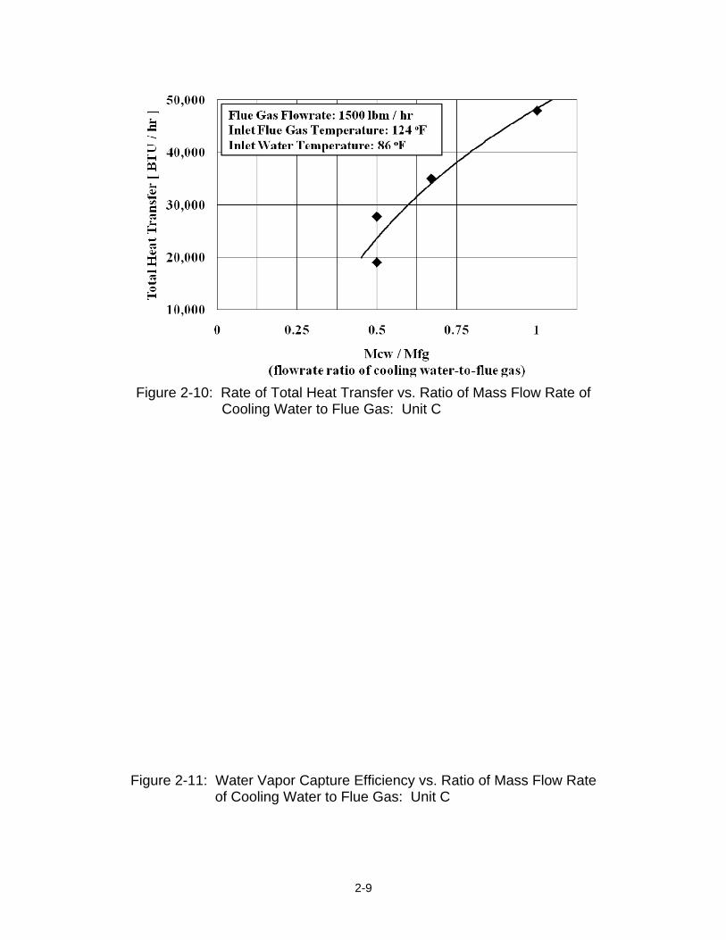
During the tests at Unit C, the slip stream of flue gas used in the tests was
extracted from the boiler’s flue gas duct immediately downstream of the wet FGD. This
resulted in flue gas inlet temperatures to the heat exchangers of approximately 123°F
and inlet flue gas volume concentrations of approximately 12.2 percent. Inlet cooling
water temperature was approximately 85°F. Four heat exchangers, with a cumulative
heat exchanger surface area of 56 ft2, were used during this sequence of tests, and
Figure 2-9 shows typical axial profiles of cooling water and flue gas temperature. The
total rate of heat transfer increased by 105 percent and the condensation efficiency
increased by 37 percent as the cooling water to flue gas flow rate ratio increased from
0.5 to 1.0 (Figures 2-10 and 2-11). This is similar to the findings for the data from Boiler
B, where the total rate of heat transfer and the condensation efficiency both increased
strongly with increasing values of cooling water to flue gas flow rate ratio.
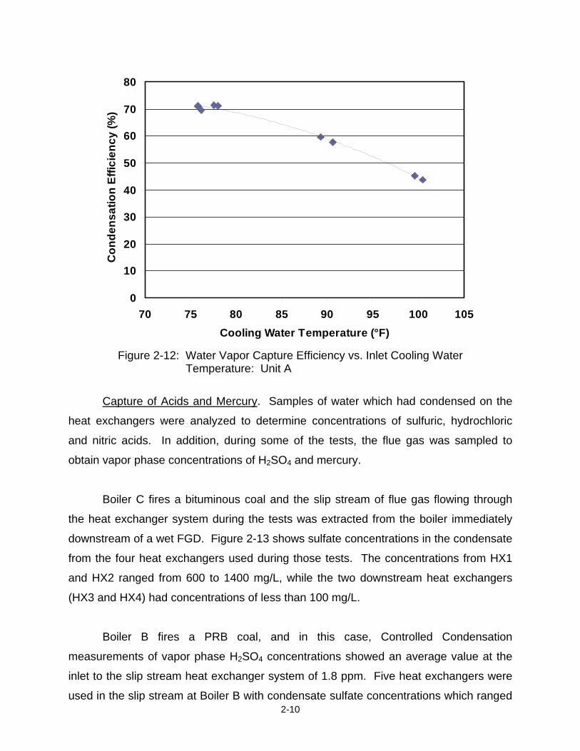
Cooling water temperature also impacts water vapor condensation efficiency and
heat transfer, with both parameters increasing as inlet cooling water temperature
decreases (Figure 2-12).
Figure 2-9: Flue Gas and Cooling Water Temperature Profiles: Unit C
2-9
Figure 2-10: Rate of Total Heat Transfer vs. Ratio of Mass Flow Rate of Cooling Water to Flue Gas: Unit C
Figure 2-11: Water Vapor Capture Efficiency vs. Ratio of Mass Flow Rate of Cooling Water to Flue Gas: Unit C
2-10
0
10
20
30
40
50
60
70
80
70 75 80 85 90 95 100 105Cooling Water Temperature (°F)
Con
dens
atio
n Ef
ficie
ncy
(%)
Figure 2-12: Water Vapor Capture Efficiency vs. Inlet Cooling Water Temperature: Unit A
Capture of Acids and Mercury. Samples of water which had condensed on the
heat exchangers were analyzed to determine concentrations of sulfuric, hydrochloric
and nitric acids. In addition, during some of the tests, the flue gas was sampled to
obtain vapor phase concentrations of H2SO4 and mercury.
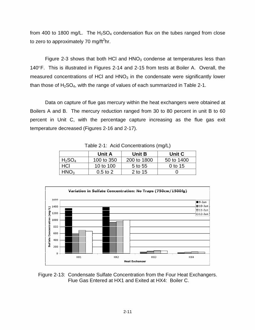
Boiler C fires a bituminous coal and the slip stream of flue gas flowing through
the heat exchanger system during the tests was extracted from the boiler immediately
downstream of a wet FGD. Figure 2-13 shows sulfate concentrations in the condensate
from the four heat exchangers used during those tests. The concentrations from HX1
and HX2 ranged from 600 to 1400 mg/L, while the two downstream heat exchangers
(HX3 and HX4) had concentrations of less than 100 mg/L.
Boiler B fires a PRB coal, and in this case, Controlled Condensation
measurements of vapor phase H2SO4 concentrations showed an average value at the
inlet to the slip stream heat exchanger system of 1.8 ppm. Five heat exchangers were
used in the slip stream at Boiler B with condensate sulfate concentrations which ranged
2-11
from 400 to 1800 mg/L. The H2SO4 condensation flux on the tubes ranged from close
to zero to approximately 70 mg/ft2hr.
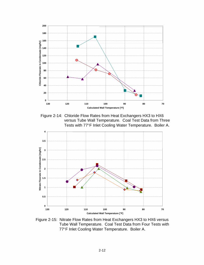
Figure 2-3 shows that both HCl and HNO3 condense at temperatures less than
140°F. This is illustrated in Figures 2-14 and 2-15 from tests at Boiler A. Overall, the
measured concentrations of HCl and HNO3 in the condensate were significantly lower
than those of H2SO4, with the range of values of each summarized in Table 2-1.
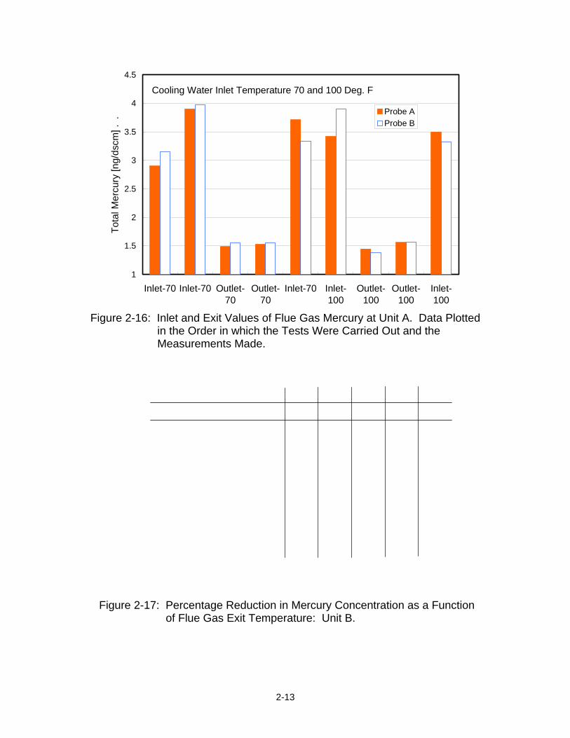
Data on capture of flue gas mercury within the heat exchangers were obtained at
Boilers A and B. The mercury reduction ranged from 30 to 80 percent in unit B to 60
percent in Unit C, with the percentage capture increasing as the flue gas exit
temperature decreased (Figures 2-16 and 2-17).
Table 2-1: Acid Concentrations (mg/L)
Unit A Unit B Unit C H2SO4 100 to 350 200 to 1800 50 to 1400 HCl 10 to 100 5 to 55 0 to 15 HNO3 0.5 to 2 2 to 15 0
Figure 2-13: Condensate Sulfate Concentration from the Four Heat Exchangers. Flue Gas Entered at HX1 and Exited at HX4: Boiler C.
2-12
0
0.5
1
1.5
2
2.5
3
3.5
4
708090100110120130Calculated Wall Temperature [°F]
Nitr
ate
Flow
rate
in C
onde
nsat
e [m
g/hr
]
Test 0731BLa-CD(COAL)Test 0731BLb-CD(COAL)Test 0731BLc-CD(COAL)Test 0813BL-CD(COAL)
Concentration in Condensates Test0731BLa Test0731BLb Test0731BLc Test0813BL Dry Flue Gas Flowrate [lb/hr] 307.5 329.9 319.4 374.8
Inlet Cooling Water Temperature [F] 77.4 77.6 75.8 Coal
Inlet Flue Gas Temperature [F] 323.5 320.7 314.1
Figure 2-14: Chloride Flow Rates from Heat Exchangers HX3 to HX6 versus Tube Wall Temperature. Coal Test Data from Three Tests with 77°F Inlet Cooling Water Temperature. Boiler A.
Figure 2-15: Nitrate Flow Rates from Heat Exchangers HX3 to HX6 versus Tube Wall Temperature. Coal Test Data from Four Tests with 77°F Inlet Cooling Water Temperature. Boiler A.
2-13
Cooling Water Inlet Temperature 70 and 100 Deg. F
1
1.5
2
2.5
3
3.5
4
4.5
Inlet-70 Inlet-70 Outlet-70
Outlet-70
Inlet-70 Inlet-100
Outlet-100
Outlet-100
Inlet-100
Tota
l Mer
cury
[ng/
dscm
] . .
Probe AProbe B
Figure 2-16: Inlet and Exit Values of Flue Gas Mercury at Unit A. Data Plotted in the Order in which the Tests Were Carried Out and the Measurements Made.
Figure 2-17: Percentage Reduction in Mercury Concentration as a Function
of Flue Gas Exit Temperature: Unit B.
2-14
Summary and Conclusions
Data on water capture efficiency and rate of heat transfer in water-cooled heat
exchangers are presented for three coal-fired boilers, two of which utilized slip streams
of flue gas taken from flue gas ducts downstream of the ESP’s, while the flue gas slip
stream from the third boiler was taken just downstream of a wet FGD. The inlet water
vapor volume fractions were approximately the same, being 11 percent for one unit, 12
percent for the second and from 11 to 14 percent for the third unit. Cooling water inlet
temperatures averaged 93°F for one unit, 85°F for the second unit and 75 to 100°F for
the third unit. The results show a strong dependence of both total heat transfer and
water vapor capture efficiency on the flow rate ratio of cooling water to flue gas. For
flue gas from Unit B, the data show a 75 percent increase in rate of heat transfer as the
cooling water to flue gas flow rate ratio increased from 0.5 to 1.6. The rate of water
condensation capture efficiency also depended strongly on cooling water to flue gas
flow rate ratio, increasing from approximately 20 percent at mcw/mfg = 0.5 to 57 percent
at mcw/mfg = 2.12.
In the case of flue gas from Unit C, the total rate of heat transfer increased by
105 percent and the condensation efficiency increased by 37 percent as the cooling
water to flue gas flow rate ratio increased from 0.5 to 1.0.
Inlet cooling water temperature also has a strong impact on water vapor
condensation efficiency. Results presented here for a cooling water to flue gas flow rate
ratio of 2.0 show that condensation efficiency increased from 44 to 71 percent as inlet
cooling water temperature decreased from 100 to 76°F.
Sulfuric, hydrochloric and nitric acids were found in the condensed water which
collected on the surfaces of the heat exchanger tubes. Among the three boilers, the
concentrations of sulfuric acid ranged from 50 to 1800 mg/L, hydrochloric acid was
found in concentrations from 0 to 100 mg/L, and the nitric acid concentrations ranged
from 0 to 15 mg/L.
2-15
Mercury measurements were made during the tests at two of the units. The
results showed that vapor phase mercury decreased by 60 percent between the inlet
and exit of the heat exchanger system at Unit A and from 30 to 80 percent at Unit C,
with the percentage capture increasing as the flue gas exit temperature decreased.
The sulfuric acid concentrations reported here are for acid-water solutions which
deposited on heat exchanger tubes at locations where the tube wall temperatures were
lower than the local water vapor dew point temperatures. Sulfuric acid also condensed
at tube wall temperatures between the water vapor and sulfuric acid dewpoint
temperatures, however, the rates of liquid deposition were significantly lower at these
temperatures and the tests were of too short a duration for the project team to be able
to collect samples of the resulting acid-water solutions. Nevertheless, there are
indications from the literature (Ref. 3) that these higher temperature solutions have
much higher acid concentrations (and consequently cause higher corrosion rates) than
the lower temperature aqueous solutions described in this Chapter.
If the heat exchangers are water cooled, the available cooling water flow rate and
temperature will govern whether the heat exchangers are better suited for improving
unit heat rate or recovering water vapor from flue gas for use as cooling tower makeup
water. In the latter case, a likely source of cooling water will be cold boiler feedwater
leaving the steam condenser. The flow rate of cold boiler feedwater is typically about
one half of the flue gas flow rate of the unit and depending on time of year and whether
the unit uses once-through cooling or an evaporative cooling tower, the feedwater
temperature typically ranges from 85 to 110°F. Recovery of water vapor from flue gas
can be enhanced through a combination of water and air-cooled heat exchangers (Ref.
4).
For applications in which heat rate improvement is the principal concern, in order
to maximize the total rate of heat transfer rate, the flue gas heat exchangers will need to
be cooled with cooling water-to-flue gas flow ratios which are larger than 0.5 and
cooling water inlet temperatures which are lower than typical cold boiler feedwater
temperatures.
2-16
References
1. Verhoff, F.H. and J.T. Banchero, “Predicting Dew Points of Flue Gas,” Chemical Engineering Progress, Vol. 70, No. 8, pp 71-72, 1974.
2. Yen Hsiung Kiang, “Predicting Dew Points of Acid Gases,” Chemical Engineering, February 9, 1981, p. 127.
3 Abel, E., “The Vapor Phase Above the System Sulfuric Acid-Water,” Journal of Physical Chemistry, Vol. 50, No. 3, pp. 260-283, 1946.
4. Levy, E. K., C. Whitcombe, I. Laurenzi, and H. Bilirgen, “Potential Water Vapor Recovery Rates and Heat Rate Reductions Resulting from Condensation of Water Vapor in Boiler Flue Gas,” Proceedings 34th International Technical Conference on Clean Coal & Fuel Systems, Clearwater, Florida, May 31 to June 4, 2009.
3-1
CHAPTER 3
CONCENTRATIONS OF DEPOSITS OF SULFURIC ACID AND WATER ON HEAT EXCHANGER TUBES
Introduction
As boiler flue gas is reduced in temperature below the sulfuric acid dew point, the
acid first condenses as a highly concentrated solution of sulfuric acid and water. Flue
gas from coal-fired boilers also contains relatively high water vapor concentrations,
resulting in water vapor dewpoint temperatures from 100 to 135°F (37.7°C to 57.2°C),
depending on coal moisture content. For those applications in which the flue gas
temperature is reduced to temperatures below the water vapor dewpoint, the liquid
mixture of water and sulfuric acid which forms is approximately two orders of magnitude
more dilute in sulfuric acid than the highly concentrated acid solutions which form at
temperatures above the water vapor dewpoint temperature, but below the sulfuric acid
dew point temperature.
At the beginning of the project, it was thought to be very likely that the tube
materials which will be most cost effective in the high temperature region with high acid
concentrations will be different from the materials of choice in the lower temperature
region with dilute acid mixtures. Long-term laboratory corrosion tests, designed to
simulate the corrosive condensate solutions encountered in field tests carried out in the
project, were conducted to identify materials which will provide adequate service life
along with desired heat transfer and structural properties. Chemical analysis of acid
concentrations in condensed water collected during heat exchanger slip stream field
tests provided data on the concentrations of the dilute water-acid mixtures which form at
temperatures below the water vapor dew point. Information on the concentrations of
high temperature concentrated sulfuric acid-water mixtures was developed from
published literature on the thermodynamics of phase equilibrium of sulfuric acid-water
mixtures.
3-2
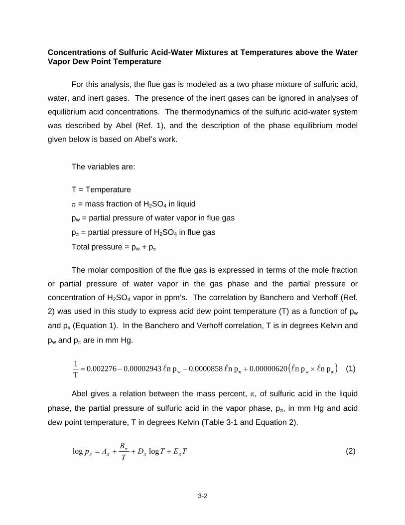
Concentrations of Sulfuric Acid-Water Mixtures at Temperatures above the Water Vapor Dew Point Temperature
For this analysis, the flue gas is modeled as a two phase mixture of sulfuric acid,
water, and inert gases. The presence of the inert gases can be ignored in analyses of
equilibrium acid concentrations. The thermodynamics of the sulfuric acid-water system
was described by Abel (Ref. 1), and the description of the phase equilibrium model
given below is based on Abel’s work.
The variables are:
T = Temperature
π = mass fraction of H2SO4 in liquid
pw = partial pressure of water vapor in flue gas
pπ = partial pressure of H2SO4 in flue gas
Total pressure = pw + pπ
The molar composition of the flue gas is expressed in terms of the mole fraction
or partial pressure of water vapor in the gas phase and the partial pressure or
concentration of H2SO4 vapor in ppm’s. The correlation by Banchero and Verhoff (Ref.
2) was used in this study to express acid dew point temperature (T) as a function of pw
and pπ (Equation 1). In the Banchero and Verhoff correlation, T is in degrees Kelvin and
pw and pπ are in mm Hg.
( )ππ p n p n 00000620.0 p n 0000858.0p n 00002943.0002276.0T1
ww llll ×+−−= (1)
Abel gives a relation between the mass percent, π, of sulfuric acid in the liquid
phase, the partial pressure of sulfuric acid in the vapor phase, pπ, in mm Hg and acid
dew point temperature, T in degrees Kelvin (Table 3-1 and Equation 2).
TETDTB
Ap πππ
ππ +++= loglog (2)
3-3
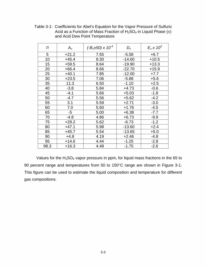
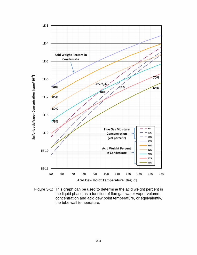
Table 3-1: Coefficients for Abel’s Equation for the Vapor Pressure of Sulfuric Acid as a Function of Mass Fraction of H2SO4 in Liquid Phase (π) and Acid Dew Point Temperature
Values for the H2SO4 vapor pressure in ppm, for liquid mass fractions in the 65 to
90 percent range and temperatures from 50 to 150°C range are shown in Figure 3-1.
This figure can be used to estimate the liquid composition and temperature for different
gas compositions.
3-4
1E‐11
1E‐10
1E‐9
1E‐8
1E‐7
1E‐6
1E‐5
1E‐4
1E‐3
50 60 70 80 90 100 110 120 130 140 150
Acid Dew Point Temperature [deg. C]
Sulfu
ric acid Vap
or Con
centration
[pp
m*10‐
6 ]
5%
10%
15%
90%
85%
80%
75%
70%
65%
90%
85%
15% 65%
80%
70%
75%
5% H 2 O65%
70%
10%
Acid Weight Percent in Condensate
Acid Weight Percent in Condensate
Flue Gas Moisture Concentration (vol percent)
Figure 3-1: This graph can be used to determine the acid weight percent in the liquid phase as a function of flue gas water vapor volume concentration and acid dew point temperature, or equivalently, the tube wall temperature.
3-5
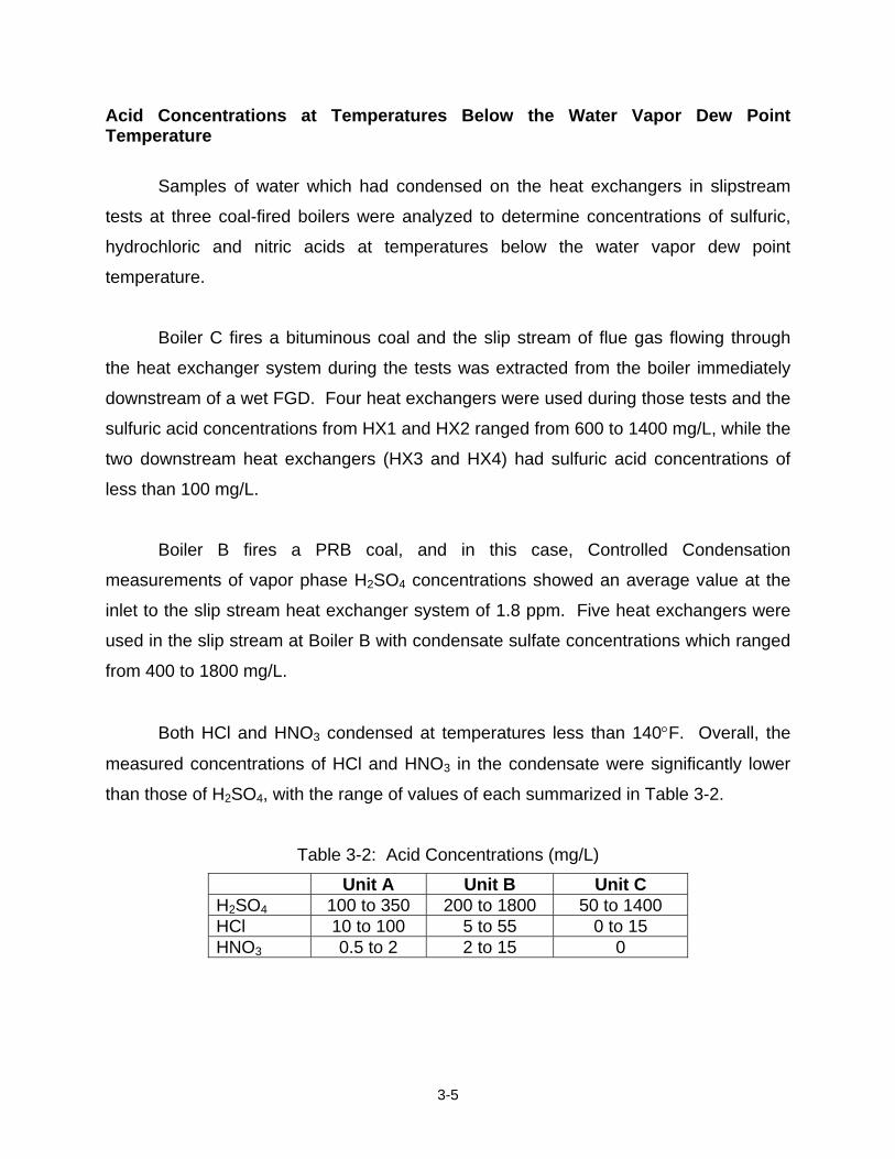
Acid Concentrations at Temperatures Below the Water Vapor Dew Point Temperature
Samples of water which had condensed on the heat exchangers in slipstream
tests at three coal-fired boilers were analyzed to determine concentrations of sulfuric,
hydrochloric and nitric acids at temperatures below the water vapor dew point
temperature.
Boiler C fires a bituminous coal and the slip stream of flue gas flowing through
the heat exchanger system during the tests was extracted from the boiler immediately
downstream of a wet FGD. Four heat exchangers were used during those tests and the
sulfuric acid concentrations from HX1 and HX2 ranged from 600 to 1400 mg/L, while the
two downstream heat exchangers (HX3 and HX4) had sulfuric acid concentrations of
less than 100 mg/L.
Boiler B fires a PRB coal, and in this case, Controlled Condensation
measurements of vapor phase H2SO4 concentrations showed an average value at the
inlet to the slip stream heat exchanger system of 1.8 ppm. Five heat exchangers were
used in the slip stream at Boiler B with condensate sulfate concentrations which ranged
from 400 to 1800 mg/L.
Both HCl and HNO3 condensed at temperatures less than 140°F. Overall, the
measured concentrations of HCl and HNO3 in the condensate were significantly lower
than those of H2SO4, with the range of values of each summarized in Table 3-2.
Table 3-2: Acid Concentrations (mg/L)
Unit A Unit B Unit C H2SO4 100 to 350 200 to 1800 50 to 1400 HCl 10 to 100 5 to 55 0 to 15 HNO3 0.5 to 2 2 to 15 0
3-6
References
1. Abel, E, “The Vapor Phase Above the System Sulfuric Acid-Water.” Journal of Physical Chemistry, Vol. 50, No. 3, pp. 260-283, 1946.
2. Banchero, J. T. and F. Verhoff, “Evaluation and Interpretation of the Vapour Pressure Data for Sulfuric Acid Aqueous Solutions with Application to Flue Gas Dew Points.” J. Institute of Fuel, pp. 76 – 86, June 1975.
4-1
CHAPTER 4
LABORATORY CORROSION TESTS OF CANDIDATE HEAT EXCHANGER TUBE MATERIALS
Introduction From slip stream tests carried out using boiler flue gas and from theoretical
analyses performed by the project team, it became apparent that as flue gas is reduced
in temperature below the sulfuric acid dew point, the acid first condenses as a highly
concentrated liquid solution of sulfuric acid and water. Flue gas from coal-fired boilers
contains relatively high water vapor concentrations, resulting in water vapor dewpoint
temperatures from 100 to 135°F, depending on coal moisture content. For those
applications in which the flue gas temperature is reduced to temperatures below the
water vapor dewpoint, the liquid mixture of water and sulfuric acid which forms on low
temperature surfaces is approximately two orders of magnitude more dilute in sulfuric
acid than the highly concentrated acid solutions which form at temperatures above the
water vapor dewpoint temperature, but below the sulfuric acid dew point temperature
(see Chapter 3).
Depending on factors such as coal composition and combustion conditions,
dilute sulfuric acid-water liquid mixtures can also contain hydrochloric and nitric acids.
The objective of this part of the project was to determine the best materials to use for
heat exchangers in each of these two distinct acid environments: (1) higher
temperature, with highly concentrated sulfuric acid and (2) lower temperature with a
dilute acid mixture, possibly containing sulfuric, hydrochloric and nitric acids.
Long-term laboratory corrosion tests, which were designed to simulate the
corrosive condensate solutions which were observed in field tests performed by the
project team, were conducted to identify materials which would provide adequate
service life along with desired heat transfer and structural properties. Chemical analysis
of acid concentrations in condensed water collected during heat exchanger slip stream
field tests provided data on the concentrations of the dilute water-acid mixtures which
4-2
form. Information on the concentrations of high temperature concentrated sulfuric acid-
water mixtures was developed by the project team from published literature on the
thermodynamics of concentrated liquid sulfuric acid.
Experimental Procedure
Long-term corrosion tests were conducted to identify materials that will provide
adequate service life in various locations of the heat exchanger. Table 4-1 lists the nine
different test conditions. The first condition was included as a screening test (prior to
receipt of all samples and completion of condensate composition and temperature
calculations) in order to make an initial assessment of the expected corrosion behavior.
The next five conditions (2 through 6) represent condensate compositions and
temperatures expected from the high temperature region of the heat exchanger, while
the remaining conditions (7 through 9) represent those expected from the low
temperature region of the heat exchanger.
Table 4-1: Summary of Condensate Compositions and Temperatures.
Condition Condensate Composition Condensate Temperature, °C
in the 60 percent H2SO4 solution at 121°C demonstrated that the stainless steels, Alloy
600, and the aluminum alloys were not suitable for the higher acid concentration
conditions. These alloys all had corrosion rates above ~ 8 mm/year. Thus, they were
not considered further for the high acid conditions. The remaining materials were then
tested first in conditions 2, 4, and 6. Materials not suitable for these conditions were not
tested in conditions 3 and 5. Similarly, all materials were tested in condition 9 first, and
only materials suitable in this condition were evaluated in conditions 7 and 8. Welded
samples were not considered for the low acid conditions because no significant adverse
effect was observed for the high acid conditions.
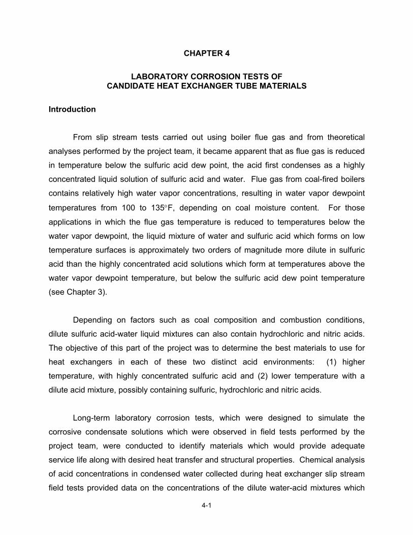
As shown in Figure 4-1, the materials were placed in test tubes that were filled
with the simulated solution and positioned within a constant temperature bath. Silicon
heating oil was used for the 115°C and 150°C tests, while peanut oil was used for the
remaining tests. Test temperatures were held to ± 1°C of the set value. A condenser
was placed on top of each test tube in order to re-condense any acid that evaporated
during the test. The test samples were completely immersed in the solution, and up to
25 individual tests were conducted in each constant temperature bath.
a) b) c)
Figure 4-1: Setup of the Long-Term Corrosion Testing. A) Side View of the Bath B) Overhead View of the Bath C) Side View of the Test Tube Showing
the Individual Components of the Test Tube Setup.
Glass St
Glass Condenser
Glass Test Tube
SS Lid
4-4
Table 4-2: Summary of Alloys Tested Under Various Conditions.
Condition→ High Acid Conditions Low Acid Conditions
Alloy↓ 1 2 3 4 5 6 7 8 9 STEELS: 1018 X X X X X X X A387 X X X X X X X Corten B X X X X X X X STAINLESS STEELS: 304 X X X X 316 X X X X AL6XN X X X X 2205 X X X Ni ALLOYS: 22 X X X X X X X X X 22-Welded X X X 59 X X X X X X 600 X X X X 625 X X X X X X 625-Welded X X X 690 X X X X X X ALUMINUM BRONZE: C-61400 X X X X X X X X C-61400-Welded X X X ALUMINUM: 3003 X X X 6061 X X X POLYMERS: FEP X X X X X X X X PTFE X X X X X X X X PEEK X X X X X TEFLON COATINGS: MP501 X X X X X Ruby Red X X X X X GRAPHITE X X X X X
The samples of each material were machined to dimensions of ¼” x ¾” x 1½”
and then ground to an 80 grit finish prior to being placed in the test solution. The
graphite was received in tube form that had a one inch outside diameter and 0.60 inch
inside diameter. Graphite test samples were one inch in length. All test samples were
weighed prior to testing and during periodic examination intervals (typically every 14
days). Fresh acid solution was provided after each inspection. The equivalent
thickness loss associated with each measured mass loss was determined by dividing
the mass loss by the density and surface area of each sample. The corrosion rate was
then determined by dividing the effective thickness loss by the exposure time. This
assumes uniform corrosion, which was justified by subsequent inspections of the
4-5
samples (as discussed in the next section). Various samples were photographed after
the tests. Select samples were used for examination by light optical microscopy (LOM).
The LOM samples were mounted in bakelite and filled with epoxy. They were then
cross sectioned and metallographically prepared to a one micron surface finish using a
diamond slurry as the final polishing step. Samples were examined and photographed
in the as-polished condition.
Results and Discussion
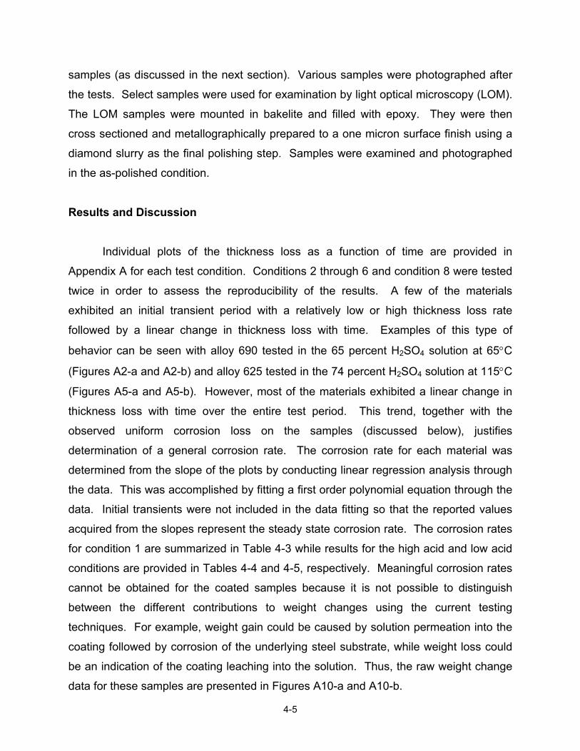
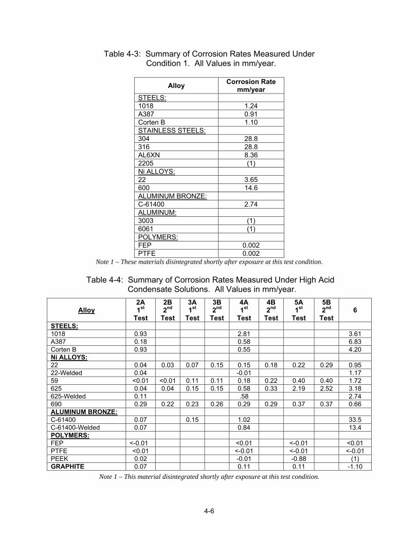
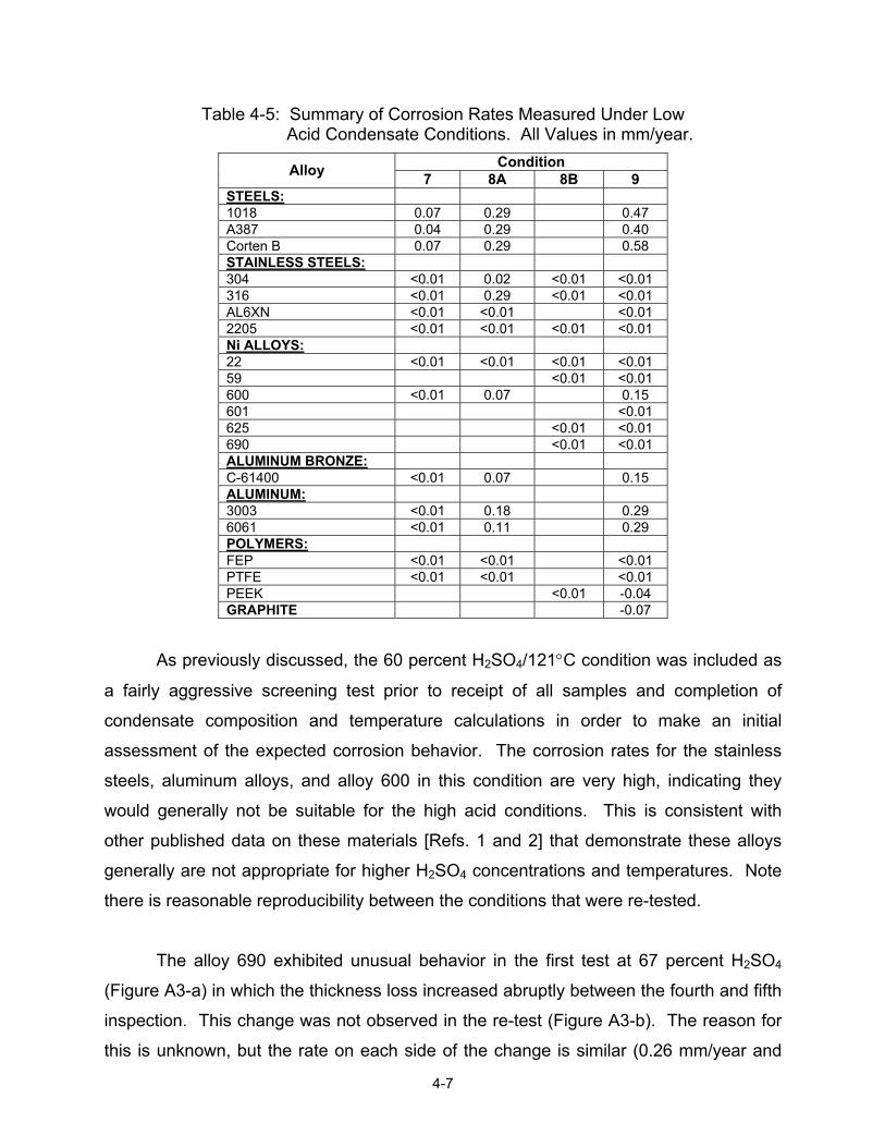
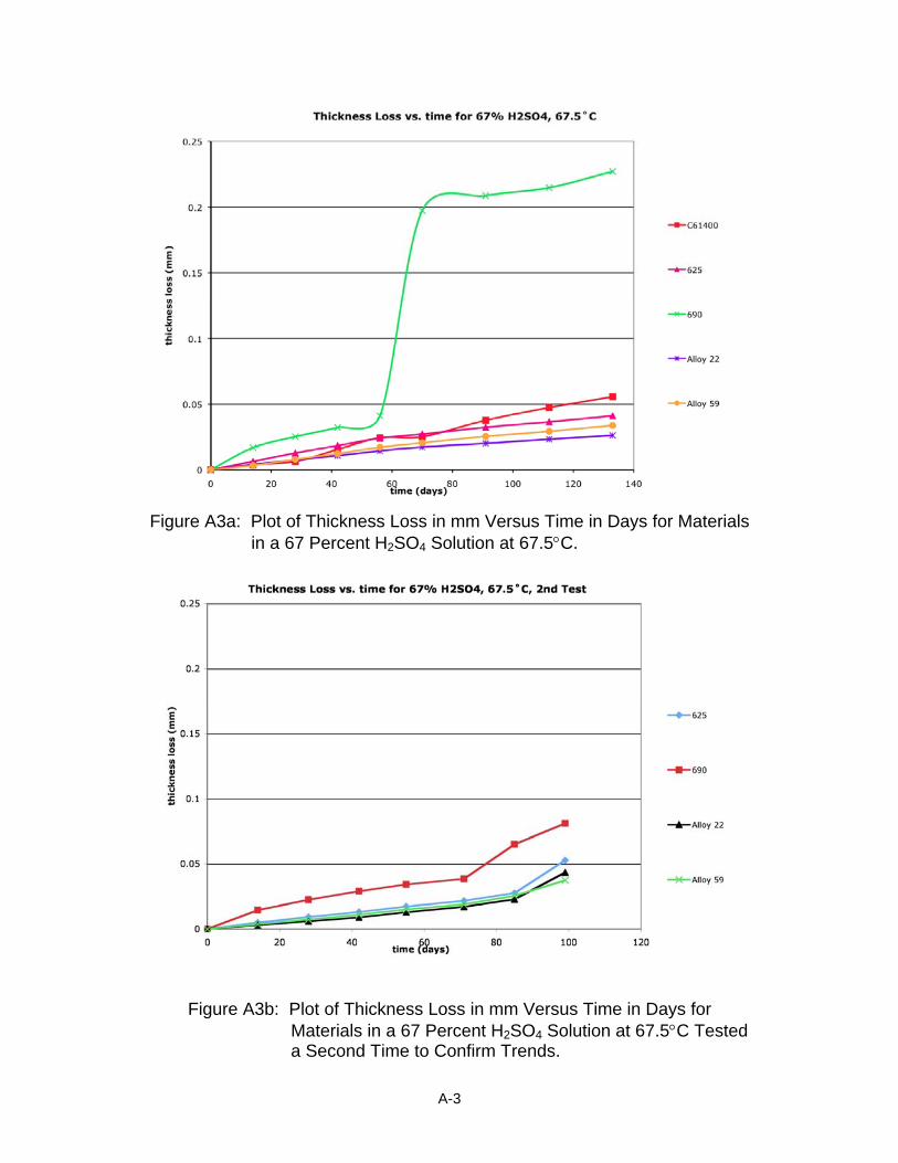
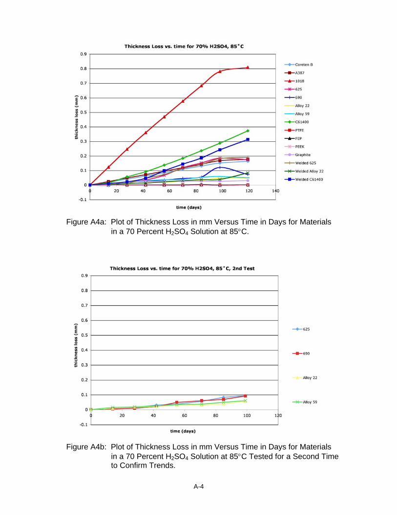
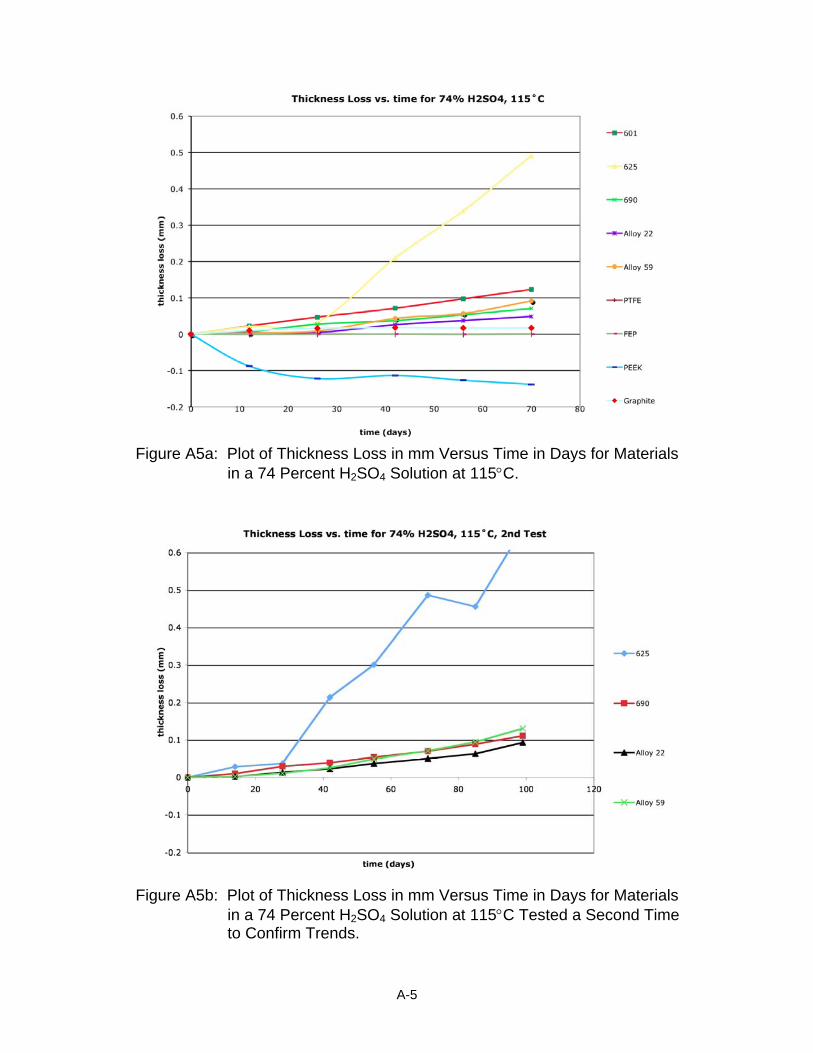
Individual plots of the thickness loss as a function of time are provided in
Appendix A for each test condition. Conditions 2 through 6 and condition 8 were tested
twice in order to assess the reproducibility of the results. A few of the materials
exhibited an initial transient period with a relatively low or high thickness loss rate
followed by a linear change in thickness loss with time. Examples of this type of
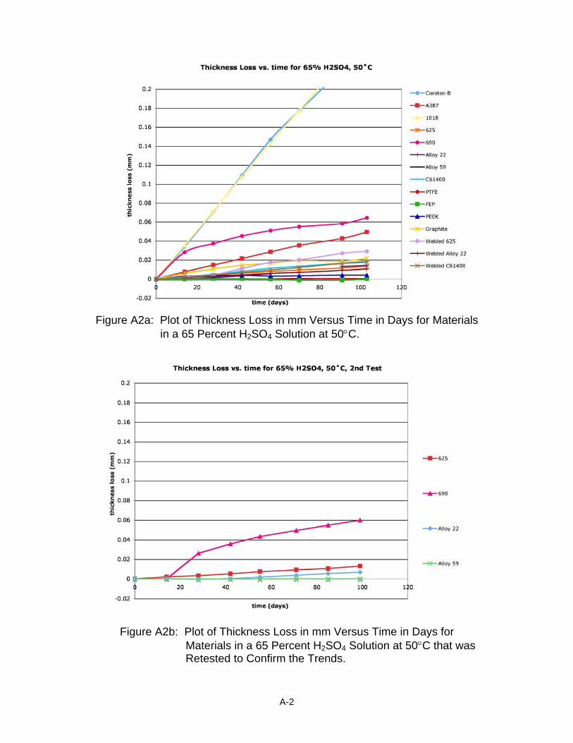
behavior can be seen with alloy 690 tested in the 65 percent H2SO4 solution at 65°C
(Figures A2-a and A2-b) and alloy 625 tested in the 74 percent H2SO4 solution at 115°C
(Figures A5-a and A5-b). However, most of the materials exhibited a linear change in
thickness loss with time over the entire test period. This trend, together with the
observed uniform corrosion loss on the samples (discussed below), justifies
determination of a general corrosion rate. The corrosion rate for each material was
determined from the slope of the plots by conducting linear regression analysis through
the data. This was accomplished by fitting a first order polynomial equation through the
data. Initial transients were not included in the data fitting so that the reported values
acquired from the slopes represent the steady state corrosion rate. The corrosion rates
for condition 1 are summarized in Table 4-3 while results for the high acid and low acid
conditions are provided in Tables 4-4 and 4-5, respectively. Meaningful corrosion rates
cannot be obtained for the coated samples because it is not possible to distinguish
between the different contributions to weight changes using the current testing
techniques. For example, weight gain could be caused by solution permeation into the
coating followed by corrosion of the underlying steel substrate, while weight loss could
be an indication of the coating leaching into the solution. Thus, the raw weight change
data for these samples are presented in Figures A10-a and A10-b.
4-6
Table 4-3: Summary of Corrosion Rates Measured Under Condition 1. All Values in mm/year.
Figure 4-6: Photographs of Various Materials from the Low Acid Test Condition.
4-13
Left: 690 ‐ 65% H2SO4 50°C (1
st test) Middle: 690 ‐ 65% H2SO4 50°C (2
nd test) Right: 690 ‐ 67% H2SO4 67.5°C (1
st test)
Left: 690 ‐ 67% H2SO4 67.5°C (2
nd test) Middle: 690 ‐ 70% H2SO4 85°C (1
st test) Right: 690 ‐ 70% H2SO4 85°C (2
nd test)
Left: 690 ‐ 74% H2SO4 115°C (1
st test) Middle: 690 ‐ 74% H2SO4 115°C (2
nd test) Right: 690 ‐ 80% H2SO4 150°C
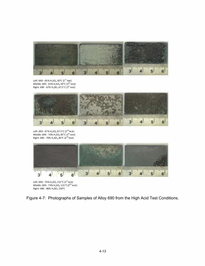
Figure 4-7: Photographs of Samples of Alloy 690 from the High Acid Test Conditions.
4-14
Left: Alloy 22 ‐ 65% H2SO4 50°C (1
st test) Middle: Alloy 22 ‐ 65% H2SO4 50°C (2
nd test) Right: Alloy 22 ‐ 67% H2SO4 67.5°C (1
st test)
Left: Alloy 22 ‐ 67% H2SO4 67.5°C (2
nd test) Middle: Alloy 22 ‐ 70% H2SO4 85°C (1
st test) Right: Alloy 22 ‐ 70% H2SO4 85°C (2
nd test)
Left: Alloy 22 ‐ 74% H2SO4 115°C (1
st test)
Middle: Alloy 22 ‐ 74% H2SO4 115°C (2nd test)
Right: Alloy 22 ‐ 80% H2SO4 150°C
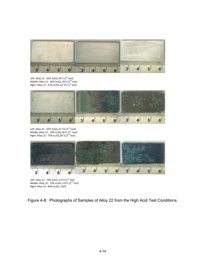
Figure 4-8: Photographs of Samples of Alloy 22 from the High Acid Test Conditions.
4-15
Left: Alloy 59 ‐ 65% H2SO4 50°C (1
st test) Middle: Alloy 59 ‐ 65% H2SO4 50°C (2
nd test) Right: Alloy 59 ‐ 67% H2SO4 67.5°C (1
st test)
Left: Alloy 59 ‐ 67% H2SO4 67.5°C (2
nd test) Middle: Alloy 59 ‐ 70% H2SO4 85°C (1
st test) Right: Alloy 59 ‐ 70% H2SO4 85°C (2
nd test)
Left: Alloy 59 ‐ 74% H2SO4 115°C (1
st test) Middle: Alloy 59 ‐ 74% H2SO4 115°C (2
nd test) Right: Alloy 59 ‐ 80% H2SO4 150°C
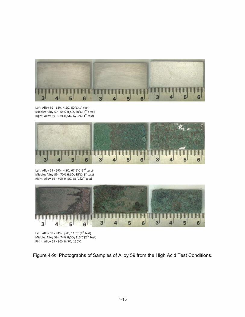
Figure 4-9: Photographs of Samples of Alloy 59 from the High Acid Test Conditions.
4-16
Left: 625 ‐ 65% H2SO4 50°C (1
st test) Middle: 625 ‐ 65% H2SO4 50°C (2
nd test) Right: 625 ‐ 67% H2SO4 67.5°C (1
st test)
. Left: 625 ‐ 67% H2SO4 67.5°C (2
nd test) Middle: 625 ‐ 70% H2SO4 85°C (1
st test)
Right: 625 ‐ 70% H2SO4 85°C (2nd test)
Left: 625 ‐ 74% H2SO4 115°C (1
st test) Middle: 625 ‐ 74% H2SO4 115°C (2
nd test) Right: 80% H2SO4 150°C
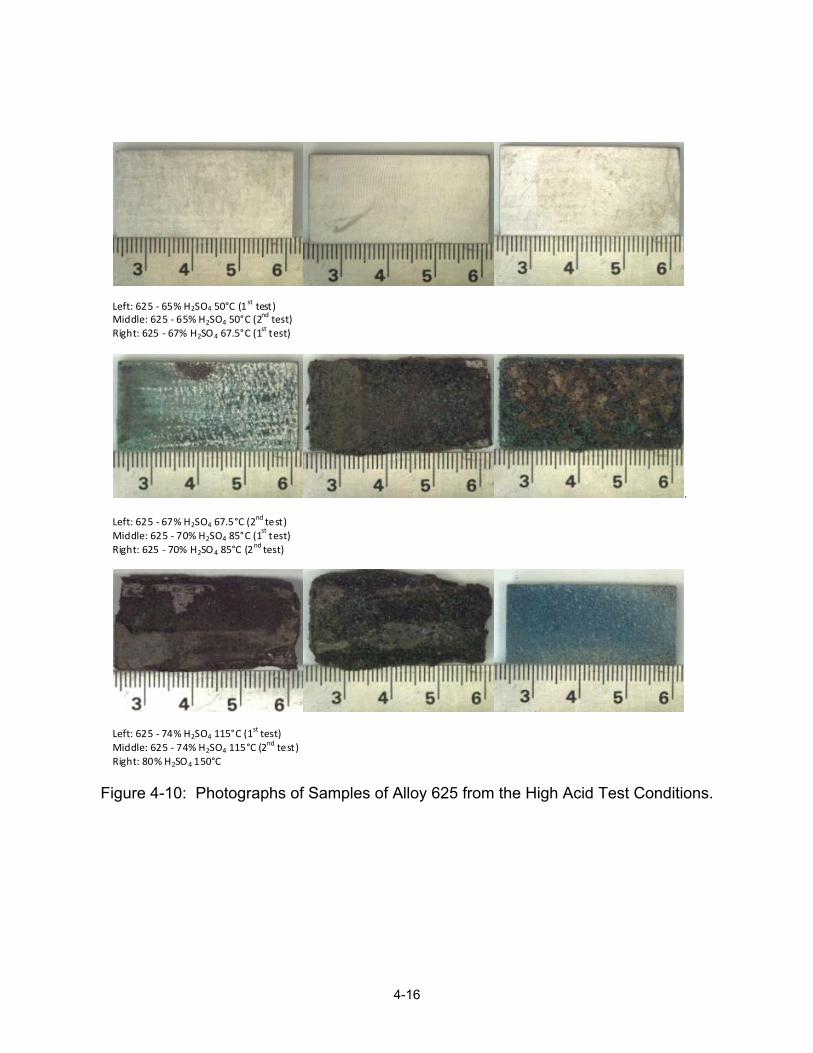
Figure 4-10: Photographs of Samples of Alloy 625 from the High Acid Test Conditions.
4-17
Sample Surface
Bakelite Mount Sample
Sample Cross‐Section
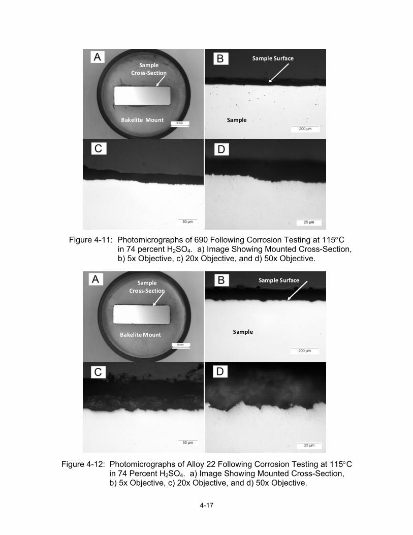
Figure 4-11: Photomicrographs of 690 Following Corrosion Testing at 115°C in 74 percent H2SO4. a) Image Showing Mounted Cross-Section, b) 5x Objective, c) 20x Objective, and d) 50x Objective.
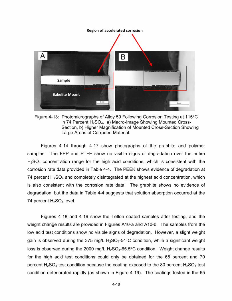
Figure 4-12: Photomicrographs of Alloy 22 Following Corrosion Testing at 115°C in 74 Percent H2SO4. a) Image Showing Mounted Cross-Section, b) 5x Objective, c) 20x Objective, and d) 50x Objective.
Sample Cross‐Section
Bakelite Mount
Sample Surface
Sample
4-18
Bakelite Mount
Sample
Region of accelerated corrosion
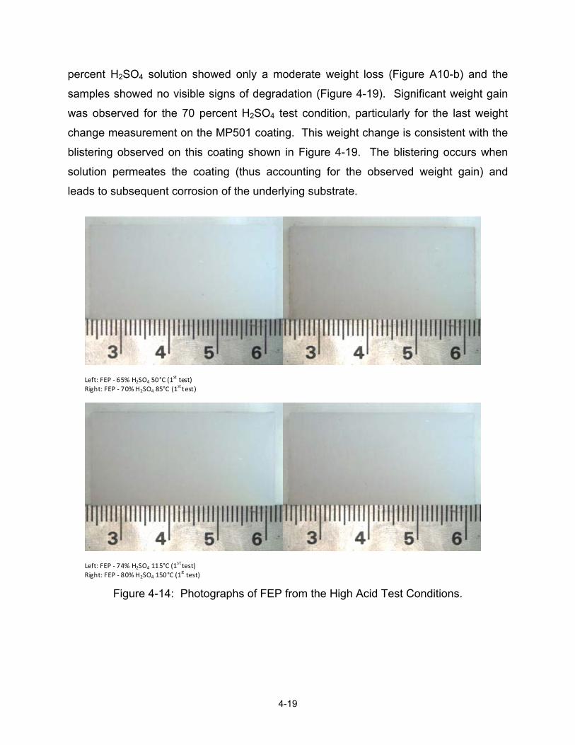
Figure 4-13: Photomicrographs of Alloy 59 Following Corrosion Testing at 115°C in 74 Percent H2SO4. a) Macro-Image Showing Mounted Cross- Section, b) Higher Magnification of Mounted Cross-Section Showing Large Areas of Corroded Material.
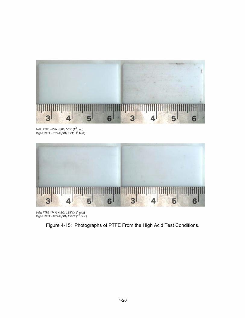
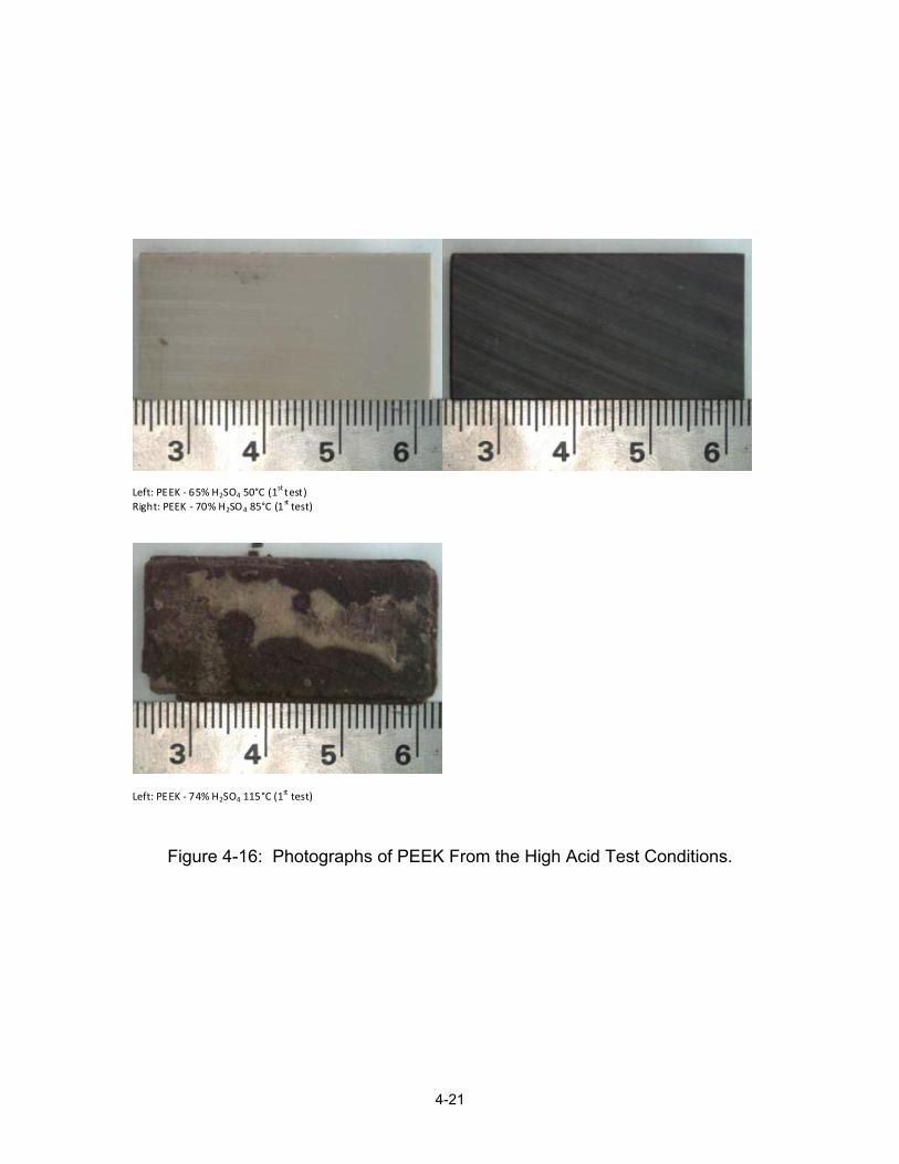
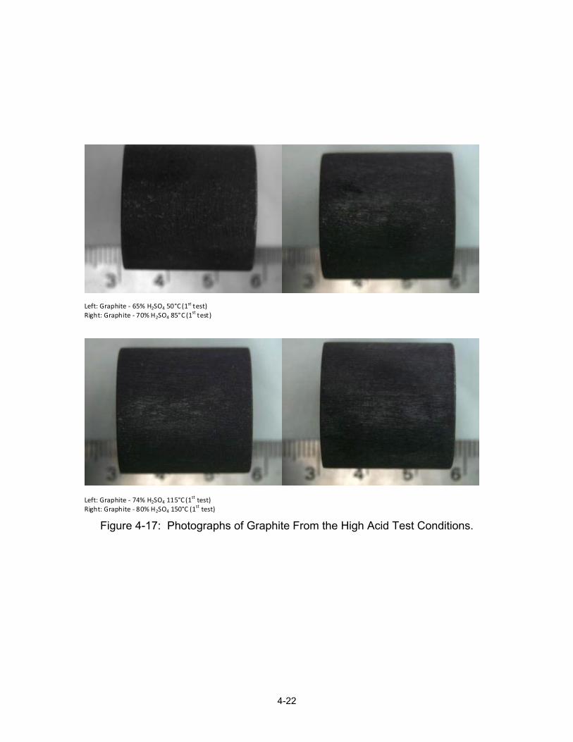
Figures 4-14 through 4-17 show photographs of the graphite and polymer
samples. The FEP and PTFE show no visible signs of degradation over the entire
H2SO4 concentration range for the high acid conditions, which is consistent with the
corrosion rate data provided in Table 4-4. The PEEK shows evidence of degradation at
74 percent H2SO4 and completely disintegrated at the highest acid concentration, which
is also consistent with the corrosion rate data. The graphite shows no evidence of
degradation, but the data in Table 4-4 suggests that solution absorption occurred at the
74 percent H2SO4 level.
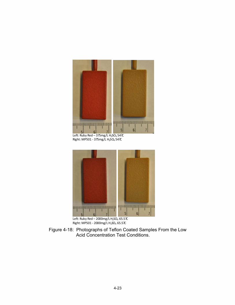
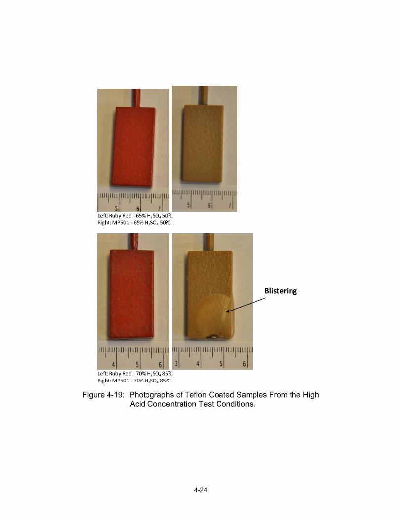
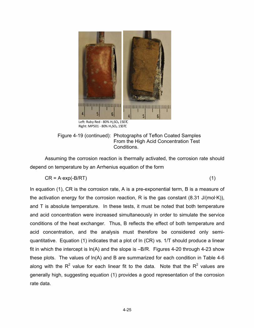
Figures 4-18 and 4-19 show the Teflon coated samples after testing, and the
weight change results are provided in Figures A10-a and A10-b. The samples from the
low acid test conditions show no visible signs of degradation. However, a slight weight
gain is observed during the 375 mg/L H2SO4-54°C condition, while a significant weight
loss is observed during the 2000 mg/L H2SO4-65.5°C condition. Weight change results
for the high acid test conditions could only be obtained for the 65 percent and 70
percent H2SO4 test condition because the coating exposed to the 80 percent H2SO4 test
condition deteriorated rapidly (as shown in Figure 4-19). The coatings tested in the 65
4-19
percent H2SO4 solution showed only a moderate weight loss (Figure A10-b) and the
samples showed no visible signs of degradation (Figure 4-19). Significant weight gain
was observed for the 70 percent H2SO4 test condition, particularly for the last weight
change measurement on the MP501 coating. This weight change is consistent with the
blistering observed on this coating shown in Figure 4-19. The blistering occurs when
solution permeates the coating (thus accounting for the observed weight gain) and
leads to subsequent corrosion of the underlying substrate.
Figure 4-14: Photographs of FEP from the High Acid Test Conditions.
Left: FEP ‐ 65% H2SO4 50°C (1
st test) Right: FEP ‐ 70% H2SO4 85°C (1
st test)
Left: FEP ‐ 74% H2SO4 115°C (1
st test) Right: FEP ‐ 80% H2SO4 150°C (1
st test)
4-20
Left: PTFE ‐ 65% H2SO4 50°C (1
st test) Right: PTFE ‐ 70% H2SO4 85°C (1
st test)
Left: PTFE ‐ 74% H2SO4 115°C (1
st test) Right: PTFE ‐ 80% H2SO4 150°C (1
st test)
Figure 4-15: Photographs of PTFE From the High Acid Test Conditions.
4-21
Left: PEEK ‐ 65% H2SO4 50°C (1
st test) Right: PEEK ‐ 70% H2SO4 85°C (1
st test)
Left: PEEK ‐ 74% H2SO4 115°C (1
st test)
Figure 4-16: Photographs of PEEK From the High Acid Test Conditions.
4-22
Left: Graphite ‐ 65% H2SO4 50°C (1
st test) Right: Graphite ‐ 70% H2SO4 85°C (1
st test)
Left: Graphite ‐ 74% H2SO4 115°C (1
st test) Right: Graphite ‐ 80% H2SO4 150°C (1
st test)
Figure 4-17: Photographs of Graphite From the High Acid Test Conditions.
Figure 4-22: Arrhenius Plot of ln(Corrosion Rate) as a Function of 1/T for
the Aluminum Bronze Alloy in the High Acid Concentration Tests.
Figure 4-23: Arrhenius Plot of ln(Corrosion Rate) as a Function of 1/T for the Steels, Aluminum Alloys, and Aluminum Bronze Alloy in the Low Acid Concentration Tests.
‐3.0
‐2.5
‐2.0
‐1.5
‐1.0
‐0.5
0.0
0.0029 0.0030 0.0031 0.0032 0.0033 0.0034 0.0035
ln (Corrosion Rate)
1/T, 1/K
1018
A387
Corten B
3003 Aluminum
6061 Aluminum
C‐61400
Linear (1018)
Linear (A387)
Linear (Corten B)
Linear (3003 Aluminum)
Linear (6061 Aluminum)
Linear (C‐61400)
‐4
‐3
‐2
‐1
0
1
2
3
4
0.0022 0.0024 0.0026 0.0028 0.003 0.0032
ln (Corrosion Rate)
1/T, 1/K
C‐61400
C‐61400 Weld
Linear (C‐61400)
Linear (C‐61400 Weld)
In(Corrosion
Rate)
In(Corrosion
Rate)
4-28
Table 4-6: Summary of ln (A), B, and R2 Values From Arrhenius Plots Provided in Figures 4-18 through 4-21.
The plots for the nickel alloys (Figure 4-20) show that all alloys except 690 have
similar slopes. This difference is probably associated with differences in composition
among the alloys. Alloys 22, 59, and 625 are all Ni-Cr-Mo alloys with similar chromium
levels while alloy 690 is essentially a Ni-Cr-Fe alloy with no molybdenum and higher
chromium. (See Table A in the Appendix for alloy compositions.) Molybdenum is an
important alloying element for stabilizing the passive film in aggressive aqueous
solutions. The corrosion rates of the Mo-bearing alloys are lower than that of alloy 690
at the lower temperatures, thus leading to the higher B values in Table 4-6. The
corrosion rate of alloy 690 exhibits less dependence on temperature and shows lower
corrosion rates at the two most aggressive test conditions, which may be attributed to
the higher chromium content of the alloy. It is difficult to draw any similar correlations
with the data for the steels. It should be noted that the carbon and low alloy steels are
known to exhibit a decrease in corrosion rate with increasing acid concentration within
the range of 60 to 70 percent H2SO4. For example, Fontana [1] has demonstrated that
the corrosion rate of steels can decrease by a factor of two at ambient temperature
Alloy Ln(A) B, J/mol R2
High Acid Conditions
1018 Steel 5.61 14,700 0.81
A387 Steel 13.7 41,740 0.99
Corten B Steel 6.42 18,620 0.61
Alloy 22 9.42 33,740 0.95
Alloy 59 15.5 51,980 0.91
Alloy 625 16.4 51,660 0.95
Alloy 625 Welded 11.4 36,090 0.99
Alloy 690 2.71 11,520 0.86
C‐61400 24.1 72,370 0.99
C‐61400 Welded 19.5 59,280 0.99
Low Acid Conditions
1018 Steel 11.7 35,160 0.99
A387 Steel 14.9 44,100 0.99
Corten B Steel 12.9 38,100 0.99
3003 Aluminum 21.8 64,460 0.99
6061 Aluminum 20.5 61,470 0.99
C‐61400 15.7 49,540 0.99
4-29
when the acid concentration is increased from 60 percent to 70 percent H2SO4. Thus,
equation (1) may not provide an accurate representation for steels under these test
conditions due to this effect. Note that two of the steel alloys have the lowest R2 values
in Table 4-6. At acid concentrations below approximately ten percent, previous results
presented by Fontana [Ref. 1] have shown that the corrosion rate of steel increases with
increasing acid concentration. This is consistent with the data in Table 4-6 for the low
acid conditions in which the steels have similar ln(A) and B values. Note that the Al
alloys also have similar ln(A) and B values.
The results presented here can be compared to available data on similar
materials and also provide useful information on newer alloys (e.g., alloys 22, 690, and
59) that can be used for material selection purposes. Previously published data [Ref. 2]
have shown that carbon and low alloy steels (i.e., similar to the 1018, A387, and Corten
B alloys investigated in this work) are known to provide adequate corrosion protection in
sulfuric acid near room temperature at acid concentrations above ~ 70 percent H2SO4.
Data published on the corrosion rates of steels under these conditions are typically in
the range of 0.1 to 0.5 mm/year [Refs. 1 and 2]. Steels are rapidly attacked at lower
acid concentrations and higher temperatures. Although acid concentrations above 70
percent H2SO4 are of interest for this application, the temperature is too high (> 115°C)
for steels to provide adequate protection. Moderate corrosion rates were observed at
the lower acid concentrations tested in this program, but the rate of 0.40 to 0.58
mm/year in the 2000 mg/L solution is too high to warrant the use of steels. Published
data on stainless steels [Ref. 2] show that these alloys are generally able to maintain
protective passive scales at temperatures below 40°C and acid concentrations below
about 1 percent and above 93 percent H2SO4. The alloys will undergo active corrosion
at intermediate acid concentrations and higher temperatures. This is consistent with the
results from this program which exhibited very low corrosion rates at low acid/low
temperature conditions and poor corrosion resistance at the high acid/high temperature
conditions. Of the stainless steels investigated in this work for the high acid conditions,
alloy AL6XN exhibited the lowest corrosion rate, which can be attributed to its high
chromium content (20 to 22 wt percent) and presence of molybdenum (6 to 7 wt
percent), each of which stabilize the protective surface scale. All of the remaining
4-30
materials showed very low corrosion rates at the low acid conditions. There is little
reported experience on the use of aluminum alloys for handling sulfuric acid, and the
corrosion rates were observed to increase with increasing acid concentration and
temperature. In contrast, the remaining materials showed negligible corrosion rates
under all the low acid conditions, so it is difficult to justify the use of aluminum alloys for
this application. Of the remaining alloys, conventional 304 stainless steel would be an
optimum choice for the low acid conditions. This alloy is less expensive than the nickel
alloys, showed negligible corrosion rates over the entire solution composition range, is
readily available and easy to fabricate by conventional manufacturing methods.
The two Teflon coatings tested do not appear to be candidate materials for this
application. While only a moderate weight gain was observed for the 375 mg/L H2SO4
solution, this may be evidence of solution permeation through the coating that can lead
to subsequent corrosion of the underlying substrate. In addition, the weight loss rate for
the 2000 mg/L H2SO4 was significant, which may be a sign of the coating leaching into
the solution under this more aggressive condition. The coatings also showed evidence
of permeation and failure under the high acid test conditions.
Corrosion data published to date indicate that nickel alloys, the polymer materials,
and graphite are all known to exhibit good resistance to sulfuric acid [Refs. 1 and 2].
However, the results shown here indicate there are important differences among the
materials considered for the conditions of interest to this application. Alloy 625 is often
used to handle sulfuric acid. Data from Reference 2 indicate this alloy exhibits
corrosion rates below 0.5 mm/year at temperatures below ~85°C and acid
concentrations from 0 to 70 percent H2SO4. The corrosion rates become appreciable
above these ranges. This is consistent with the corrosion rate data shown in Table 4-4
from this work. Thus, this alloy is not preferred for this application. In contrast, results
from this work show that alloys 22, 59, and 690 exhibited lower corrosion rates over a
wider range of acid concentrations and temperatures. Alloys 22 and 59 are known to be
among the best alloys for resistance to aggressive aqueous corrosion. The good
corrosion resistance of these alloys is attributed to their high chromium content (20 – 24
wt percent) and high molybdenum concentration (12 to 16.5 wt percent). The good
4-31
performance of alloy 690 is probably a result of its high chromium content (27-31 wt
percent). Of these materials, alloys 22 and 690 are preferred because they showed the
lowest susceptibility to accelerated corrosion at the higher temperatures. Alloy 22
showed the best overall performance and is the preferred material for the high acid
conditions. This alloy is readily available and can be manufactured by conventional
manufacturing methods. The polymer materials are potential options for this application
as either protective coatings or structural materials. Of the three materials evaluated
here, the FEP and PTFE performed the best. PTFE has been reported to be free from
attack of H2SO4 over the entire composition range at temperature up to 260°C [Ref. 2],
which is consistent with the results presented here. The ultimate use of FEP and/or
PTFE as a structural material or coating would have to be justified by also considering
factors associated with reduced heat transfer (due to lower thermal conductivity), ability
to handle operating stresses (due to reduced strength), and possible increased
assembly costs (due to difficulty in manufacturing relative to engineering alloys).
Conclusions
The corrosion behavior of a wide range of materials was evaluated under low
and high acid sulfuric acid conditions that are representative of the heat exchanger
conditions. The following conclusions can be drawn from the results:
1. The corrosion rates of the engineering alloys increased with increasing acid
concentration and temperature. Except for the steels, the corrosion rate of the
engineering alloys followed an equation of the form CR = A·exp(-B/RT).
2. All materials except steels showed acceptable corrosion rates in the low acid
conditions. Of the remaining alloys, 304 stainless steel is the preferred choice for
the low acid condition due to the relatively low cost, ease of fabrication, and
negligible corrosion rates over the entire range of test conditions.
3. Teflon coatings MP501 and Ruby Red are not likely candidates for this
application due to evidence of permeation, leaching of the coating, and complete
coating failure under the most aggressive test conditions.
4-32
4. Alloys 22 and 690 along with polymeric materials FEP and PTFE showed the
best performance in the high acid conditions. The polymer materials showed no
significant signs of degradation over the entire acid composition range. Alloys 22
and 690 exhibited increased corrosion rates with increasing acid concentration
and temperature, but should provide acceptable performance up to 74 percent
H2SO4 and 115°C where the corrosion rates are less than 0.4 mm/year.
5. The corrosion rates of alloys 22 and 625 that contained welds were not
significantly different than the wrought alloys.
6. Alloy 22 is the preferred alloy for the high acid concentration due to its low
corrosion rate, availability, and ability to be readily fabricated.
References
1. S.K. Brubaker, Corrosion by Sulfuric Acid, ASM Handbook, Volume 13, Corrosion, ASM International, Materials Park, OH, 2001, pp. 1148-1154.
2. M.G. Fontana, Corrosion Engineering, McGraw-Hill Publishing, New York, NY, 1986, pp. 317-337.
5-1
CHAPTER 5
REDUCING SULFURIC ACID DEPOSITION ON HEAT EXCHANGER TUBES: MEASUREMENT OF ACID TRAP EFFECTIVENESS
Introduction
Project DE-NT0005648 was undertaken with the knowledge that sulfuric acid
corrosion of heat exchanger tubes could be a limiting factor in the cost effectiveness of
using condensing heat exchangers to recover thermal energy and condensed water
vapor from boiler flue gas. One of the project tasks involved tests to assess the
potential of reducing the flue gas acid concentration entering the heat exchangers
through use of additional surface area in the inlet region to capture a portion of the inlet
H2SO4. The concept involved use of a section of inlet duct filled with closely spaced
vertical flat plates aligned parallel to the flow direction (referred to as “acid traps” in this
report). Tests were carried out with acid traps located upstream of the first heat
exchanger (HX1), between HX1 and HX2, and both upstream and downstream of HX1.
Results of Slip Stream Tests
Tests to measure the effectiveness of acid traps in reducing flue gas sulfuric acid
concentration were performed in slip streams of flue gas extracted from a gas-fired
boiler and two coal-fired boilers. The results are described in the following sections.
Flue Gas from Gas-Fired Boiler. Tests were carried out at Lehigh University’s Boiler
House using a slip stream of flue gas from a natural gas-fired boiler. Controlled
amounts of H2SO4 were injected into the flue gas slip stream upstream of the
condensing heat exchanger apparatus to simulate the H2SO4 vapor aspects of the flue
gas environment in a coal fired boiler.
The plan for this group of tests required that sulfuric acid condense on the first
heat exchanger and in the acid trap, while the tube wall surfaces of this heat exchanger
and acid trap were at temperatures above the water vapor dew point. The tube wall
surfaces of most of the remaining heat exchangers were to be at temperatures below
5-2
the water vapor dew point, leading to condensation of water vapor and sulfuric acid and
the formation of relatively dilute acid-water solutions on the downstream heat
exchangers. Figure 5-1 shows the physical arrangement of the heat exchangers and
the acid trap and Table 5-1 gives the corresponding surface areas.
Figure 5-1: Diagram of Heat Exchanger Arrangement Used for Tests at Natural Gas-Fired Boiler
Table 5-1: Surface Areas of Heat Exchangers and Acid Trap
Heat Exchanger Surface Area [ft2]
1 7.5 Acid Trap 66.0
2 17.5 3 12.5 4 17.5 5 17.5
Seven tests were performed with the physical arrangement shown in Figure 5-1.
Sulfur trioxide (SO3), formed in a catalytic reactor, was injected into the flue gas
upstream of the first heat exchanger to simulate flue gas from a coal-fired boiler. Once
in contact with flue gas, the SO3 reacted with H2O vapor to form H2SO4 vapor. In some
tests, duct heaters located upstream of the acid injection location preheated the flue gas
to temperatures above the sulfuric acid dew point, thus preventing acid condensation
upstream of the inlet of the first heat exchanger.
Gypsum Deposition. There is carryover of acid mist containing fine gypsum
(CaSO4) particles in the flue gas from the wet FGD at Unit C. This is of concern
because of the potential for having gypsum deposits fouling the heat exchangers and
thus decreasing rates of heat and mass transfer and increasing pressure drop. The
condensate draining from the heat exchangers was analyzed to determine the
concentrations of calcium in the various condensate streams. The results are shown in
Figure 5-15 for one set of process conditions. These data indicate that calcium
deposited throughout the heat exchanger array, but with the largest calcium
concentration appearing in the condensate draining off of HX1. The data also show that
use of an acid trap upstream of the first heat exchanger (Configuration II) resulted in a
60 percent reduction in calcium concentration on HX1. (Note that while the data on
calcium concentrations in the condensate provide evidence that gypsum penetrated the
heat exchanger array, the data do not indicate the extent to which gypsum deposits
would have developed on the heat exchanger tubes over the long term.)
5-14
0
1000
2000
3000
4000
5000
6000
0 1 2 3 4 5
HX #
Cal
cium
[ug/
L] .
No TrapOne Trap
1 Trap
No Trap
Figure 5-15: Calcium Concentration in Condensate on Four Heat Exchangers: Comparison of No Trap with Trap 1
Conclusions
Tests at Gas-Fired Boiler. Acid deposition tests were performed with flue gas from a
natural gas-fired boiler, with sulfur trioxide being injected into the flue gas to form a
sulfuric acid vapor component in the flue gas. Flue gas inlet temperature and flue gas
and cooling water flow rates were adjusted to establish tube wall temperatures which
were above the water vapor dew point temperature and below the sulfuric acid dew
point temperature in the first heat exchanger and acid trap. Controlled Condensation
measurements of flue gas SO3 concentrations at the inlet and exit of the acid trap
showed an average SO3 reduction of 13.7 percent across the acid trap in the gas-fired
boiler tests.
Tests at Unit B. The tests at Unit B were carried out with the heat exchanger
apparatus located next to one of the induced draft fans and a slip stream of flue gas
being taken at the fan discharge. As was the case with the tests at the gas-fired boiler,
flue gas and cooling water flow rates were adjusted to establish tube wall temperatures
5-15
which were above the water vapor dew point temperature and below the sulfuric acid
dew point temperature in the first heat exchanger and acid trap.
Tests performed with SO3 injected into the flue gas upstream of the first heat
exchanger, resulted in inlet SO3 concentrations which were as high as 39 ppm. The
acid trap reduced the SO3 vapor phase concentration entering the first heat exchanger
by 10.2 percent. In addition, the overall reduction of flue gas SO3 concentration
between the inlet of the first heat exchanger and the exit of the last heat exchanger was
24.1 percent.
Tests at Unit C. In the tests at Unit C, the heat exchanger system was installed just
downstream of a wet FGD, with acid trap temperatures just below the water vapor dew
point temperature.
The test data show that the presence of an acid trap resulted in reduced sulfuric
acid flux on heat exchangers positioned just downstream of the trap, with reductions in
flux averaging 33 and 42 percent for the two cases tested. Measurements of total acid
flow rates showed that the trap located upstream of the first heat exchanger captured
from 62 to 76 percent of the total sulfuric acid which was captured by the heat
exchanger system.
There is carryover of acid mist containing fine gypsum (CaSO4) particles in the
flue gas from the wet FGD at Unit C. This is of concern because of the potential for
having gypsum deposits fouling the heat exchangers and decreasing rates of heat and
mass transfer and increasing pressure drop. The condensate draining from the heat
exchangers was analyzed to determine the concentrations of calcium in the various
condensate streams. The data indicate that calcium deposited throughout the heat
exchanger array, but with the largest calcium concentration appearing in the
condensate draining from HX1. The data also show that use of an acid trap upstream
of the first heat exchanger resulted in a 60 percent reduction in calcium concentration
on HX1.
5-16
Final Comments. In summary, the results from the three boilers show that acid traps
can be effective at reducing the quantities of sulfuric acid flowing into the heat
exchangers. At temperatures above the water vapor dewpoint, the acid traps reduced
the vapor phase acid concentrations entering the heat exchangers just downstream of
the traps by 10.2 to 13.7 percent. At temperatures at or below the water vapor dew
point, the presence of an acid trap reduced the sulfuric acid flux on the heat exchanger
positioned just downstream of the trap by 33 to 42 percent.
Corrosion test data described elsewhere in this report show that rates of
corrosion increase with increasing sulfuric acid concentration for some materials. This
suggests that acid traps can be useful in reducing rates of heat exchanger tube wall
corrosion. The data also show acid traps can be effective at reducing amounts of
sulfuric acid which pass through the heat exchanger array into the downstream
ductwork, which is of potential importance for acid emissions control, component life
and maintenance costs.
6-1
0
1
2
3
4
5
6
7
8
9
10
0 0.1 0.2 0.3 0.4 0.5 0.6 0.7 0.8 0.9 1
Normalized Cumulative HX Area
Moi
stur
e Fr
actio
n in
Flu
e G
as [v
ol%
wet
]
Measured yH2OPredicted yH2O
Test 0108Inlet Wet Flue Gas Flowrate = 439.9 lb/hrInlet Wet Flue Gas Temp. = 261.9 FInlet Moisture Fraction = 7.7 vol%wetCooling Water Flowrate = 605.2 lb/hrInlet Cooling Water Temperature = 49.4 F
Test 0731 BlaInlet Wet Flue Gas Flowrate = 336.1 lb/hrInlet Wet Flue Gas Temp. = 299.1 FInlet Moisture Fraction = 13.5 vol%wetCooling Water Flowrate = 820.81 lb/hrInlet Cooling Water Temperature = 76.8 F
Fuel : CoalConfig. : Bare TubeWet Gas Flowrate : 336 - 424 lb/hrFlue Gas Temp. : 286-304 FCooling Water Flowrate : 620-891 lb/hrCooling Water Temp. : 75.8-100.5 FAveraged Error : 2.6 %
Figure 6-2: Variations of Flue Gas and Cooling Water Temperatures with Distance through the Heat Exchanger: Comparison of Predicted and Measured Values
Figure 6-3: Comparison of Predicted and Measured Values of
Condensation Efficiency vs. Cooling Water Temperature
6-3
0
10
20
30
40
50
60
70
80
90
100
0 10 20 30 40 50 60 70 80 90 100
Measured Condensation Efficiency [wt%]
Pre
dict
ed C
onde
nsat
ion
Effi
cien
cy [w
t%]
Fuel : CoalConfig. : Bare TubeWet Gas Flowrate : 336 - 424 lb/hrInlet Moisture Fraction : 11.9 - 14.4 vol%wetInlet Flue Gas Temp. : 263-323 FCooling Water Flowrate : 620-1460 lb/hrInlet Cooling Water Temp. : 75.8-100.5 FAveraged Error : 2.5 %
+10%
-10%
Figure 6-4: Comparison of Predicted and Measured Values of Condensation Efficiency
The computer software, which is described in the following section, was then
used to perform analyses to estimate how much flue gas moisture it would be practical
to recover from boiler flue gas, the size and cost of the heat exchangers, and flue gas
and cooling water pressure drops.
Heat Exchanger Simulation Method
The heat and mass transfer model used for the simulations assumes a counter-
flow bare-tube heat exchanger in a duct, with cooling water flowing through the tubes
and the gas/water vapor mixture flowing on the outside of the tubes (Reference 1). The
software solves finite difference forms of the equations for conservation of energy in the
flue gas
( ) dATThdTCpm igggg ∗−∗=∗∗&
and cooling water
( ) ( )[ ] ccciOHmfgigg dTCpmdA yykhTTh2
∗∗=−∗+− &
6-4
along with the Colburn-Hougen equation, which when condensation occurs, is used to
calculate the liquid-vapor interface temperature, Ti. In the absence of condensation, Ti
is replaced by the tube wall temperature, Tw.
( ) ( ) ( )ciOiohfgmigg TTUyyhkTTh2
−=−∗+−
In addition to the governing equations, correlations were used to approximate the
heat and mass transfer coefficients. The heat transfer coefficient for the flue gas side
was calculated using a correlation for Nussult number for bare tube heat exchangers.
25.0
s
36.0mmax,DD Pr
PrPrReCNu ⎟⎟⎠
⎞⎜⎜⎝
⎛∗∗=
where C and m are functions of Reynolds number. The respective heat transfer
coefficient for the cooling water side is calculated from
( )
( )1Pr8f7.121
Pr1000DRe8f
Nu67.0
5.0D
−⎟⎠⎞
⎜⎝⎛+
−∗⎟⎠⎞
⎜⎝⎛
=
where the parameter f is a function of ReD. The mass transfer coefficient for water
vapor in flue gas is related to the heat transfer coefficient through the following
expression.
67.0glmgg
ohgm LeyMCp
Mhk 2
∗∗∗
∗=
The final correlation used is the Antoine equation, which is used to calculate
interfacial mole fractions of water vapor.
total
cTba
i Pey
i⎟⎟⎠
⎞⎜⎜⎝
⎛+
−
=
Numerical analyses were performed in a step-wise fashion in the axial direction
by discretizing the heat transfer surface area into infinitesimal cells. Inlet flue gas
temperature and mass flow rate were specified, as well as cooling water mass flow rate,
inlet vapor fraction, and inlet cooling water temperature. Because the simulation
6-5
models a cross-flow, counter-flow heat exchanger, the exit cooling water temperature is
unknown initially, although it is needed for performing the simulation. To handle this,
the code uses a “goal-seek” type analysis, where the cooling water exit temperature is
arbitrarily assigned. The code subsequently steps through the heat exchanger one
“cell” at a time, where each cell’s exit conditions represent the inlet of conditions of the
subsequent cell. When the heat exchanger exit conditions are calculated, the
calculated cooling water inlet temperature is compared to the known cooling water inlet
temperature. At this point, the process is iterated with a new estimated exit cooling
water temperature until the calculated and specified inlet cooling water temperatures
agree to within 1 percent.
Design of Full-Scale Heat Exchangers
Heat Exchanger Dimensions and Process Parameters. The heat exchanger
simulation code was used to explore alternate designs for full-scale heat exchangers.
The general heat exchanger configuration consists of bare wall tubes in a cross flow-
counter flow arrangement in a rectangular duct with cooling water flowing inside the
tubes and flue gas around the tubes (Figure 6-5). Key process and design parameters
include heat transfer surface area, choice of tube material, inlet flue gas temperature
and water vapor concentration, inlet cooling water temperature and inlet flue gas and
cooling water flow rates.
Figure 6-5: Two Dimensional Diagram of Heat Exchanger: Side View.
6-6
The results described in this Chapter are for a 550 MW unit with a 6 million
lbm/hr flue gas flow rate. Simulations were performed early in this task to identify tube
bundle dimensions which would provide a good compromise between heat transfer and
pressure drop. The result was an in-line heat exchanger in a 40 ft wide by 40 ft high
square duct. The tube bundle consists of 2.375 inch OD tubing with a 0.218 inch wall
thickness and with a 6.17 inch center-to-center transverse tube spacing and a center-to-
center 2.97 inch longitudinal tube spacing.
Heat exchanger capital costs were estimated from tube material costs and costs
for fabrication and installation. Flue gas pressure drops were calculated using standard
correlations for pressure drops in tube bundles and cooling water pressure drops were
taken from correlations for pressure drops in cylindrical tubes. These were then used to
estimate the incremental power requirements for the induced draft (ID) fan and cooling
water pump. Unless otherwise noted, annual power costs are based on full load
operation for 7,000 hrs per year at $50/MWh.
Choice of Tube Material. The laboratory tube material corrosion measurements
described in Chapter 4 identified 304 stainless steel as the best candidate for heat
exchangers which operate at temperatures below the water vapor dew point
temperature and Teflon and Alloy 22 for heat exchangers which operate at
temperatures above the water vapor dew point temperature, but below the sulfuric acid
dew point temperature. Table 6-1 summarizes the thermal conductivities, tensile
strengths and cost/ft of tubing with a 2.375” OD and 0.218” thick wall.
Table 6-1 shows that because of its relatively low cost and high tensile strength
and thermal conductivity, 304 SS is the preferred choice for heat exchanger tubing at
temperatures below the water vapor dew point.
At locations in the flue gas upstream of the water vapor dewpoint, the choice is
between Teflon and Alloy 22. While Teflon is the less expensive of the two materials
per foot of tubing, it has extremely low values of thermal conductivity and tensile
strength compared to Alloy 22. Heat exchanger design calculations were carried out to
determine which would be the more cost effective for the high temperature flue gas
cooler application.
Figure 6-6 shows predicted temperature profiles in a heat exchanger with a total
surface area of 300,000 ft2. Flue gas enters from the left (at SA = 0 ft2) at 300°F and
cooling water enters from the right at 100°F. The wall and dew point temperatures
cross at approximately 240,000 ft2 from the flue gas inlet, causing water vapor to
condense over the region from 240,000 to 300,000 ft2. It was assumed the tubes are
made from Alloy 22 for tube wall temperatures above the local water vapor dew point
temperature and 304 SS for tube wall temperatures below the local water dew point
temperature.
Figure 6-6: Temperature Profiles Through an Alloy 22 Heat Exchanger
6-8
Figure 6-7 shows predicted temperature profiles in a Teflon (PTFE) heat
exchanger having the same dimensions, gas and water flow rates and inlet
temperatures as the heat exchanger in Figure 6-6. The extremely poor thermal
conductivity of the Teflon tube results in tube walls with high thermal resistance, which
causes relatively large temperature differences between the outer surface of the tube
wall and cooling water. For the process conditions shown, this prevents the outer wall
temperature from dropping below the dew point temperature. Thus, while the Teflon
heat exchanger would cool the flue gas, no water vapor would condense for this design
and process conditions.
Figure 6-7: Temperature Profiles Through a Teflon Heat Exchanger
Figure 6-8 compares predicted total heat transfer rate as functions of heat
exchanger surface area for Teflon and Alloy 22 heat exchangers with the same inlet
process conditions. This shows that in order to transfer the same amount of heat, the
Teflon heat exchanger would need to have approximately three times the surface area
of an Alloy 22 heat exchanger. Figure 6-9 compares predicted total heat transfer as
functions of total annual costs for the Teflon and Alloy 22 heat exchangers shown in
Figure 6-8. (Note: Annual cost is based on an annual fixed charge rate and the cost of
electric power needed to overcome the gas side and cooling water side heat exchanger
pressure drops.) This figure shows that the Teflon heat exchanger would result in a
6-9
larger total annual cost than the Alloy 22 heat exchanger for the same rate of heat
transfer. While Teflon tubing is less expensive per foot of tubing than Alloy 22 tubing, a
larger heat exchanger would be needed with Teflon and this would also result in larger
pump and fan power requirements than would be needed for the Alloy 22 heat
exchanger. (Note: The analyses described in Figures 6-7 to 6-9 are for heat
exchangers with cooling water pressures in excess of 15 psi. To avoid creep damage
to Teflon tubes with high internal pressures, thicker tube walls would be needed for
Teflon tubes than would be needed for Alloy 22 tubes. However, to facilitate direct
comparison of Alloy 22 and PTFE heat exchangers, the same tube wall thickness was
used in analyses of each. As a result, the impacts of low thermal conductivity tube
walls, when using Teflon tubes, on heat exchanger size and cost and on cooling water
and flue gas pressure drops are even larger than are shown in Figures 6-7 to 6-9.)
In summary, Alloy 22 is a better choice than Teflon for heat exchangers which
would operate at temperatures above the water vapor dew point temperature. The
relatively low thermal conductivity of Teflon would prevent water vapor condensation
with Teflon tubes. In addition, the total annual costs for a Teflon heat exchanger would
be greater than for a heat exchanger fabricated from Alloy 22.
Figure 6-8: Total Heat Transfer vs. Surface Area. Comparison of
Teflon and Alloy 22 Heat Exchangers
6-10
Figure 6-9: Total Heat Transfer vs. Annual Cost. Comparison of Teflon and Alloy 22 Heat Exchangers.
Heat Exchangers for 300°F and 135°F Inlet Gas Temperatures. There will be
separate applications for condensing heat exchangers, depending on coal type. A
boiler firing a Powder River Basin coal, with its typically low sulfur and high alkali
contents, may not need a wet SO2 scrubber, and in this case, the flue gas temperature
at the inlet of the condensing heat exchanger will be in the 300°F range with inlet water
vapor concentrations of approximately 12 volume percent range. For those applications
in which a wet FGD is needed for SO2 control (bituminous coals and some lignites
typically require wet FGD’s), the flue gas entering the condensing heat exchanger will
be saturated with water vapor and have a temperature ranging from 125 to 135°F, with
the temperature depending on coal moisture content.
Design calculations were performed for heat exchangers with 300°F and 135°F
inlet flue gas temperatures, and the corresponding capital and operating costs were
estimated. In each case, an inlet flue gas flow rate of 6 million lbm/hr and a cooling
water to flue gas flow rate ratio of 0.5 were assumed. Inlet water temperatures from 90
to 105°F were assumed. Inlet flue gas water vapor concentrations of 12 volume percent
for PRB coal and 17.2 volume percent for the wet FGD case were assumed.
6-11
Figures 6-10 to 6-12 show predicted condensation rate, condensation efficiency
and heat transfer rate as functions of inlet cooling water temperature and heat
exchanger length (or equivalently, heat exchanger surface area) for a 300°F inlet flue
gas temperature. These show the condensation process is particularly sensitive to
cooling water temperature, with predicted condensation rate doubling as cooling water
temperature decreases from 105 to 90°F.
Rates of heat transfer and condensation and condensation efficiency also
depend strongly on cooling water to flue gas flow rate ratio. Figure 6-13 shows
predicted condensation efficiencies for a 300°F flue gas inlet temperature and for a 90°F
inlet cooling water temperature and heat exchanger surface areas ranging up to
600,000 ft2. The results show the condensation efficiency increases from approximately
17 to 60 percent as Mcw/Mfg increases from 0.5 to 2.0 for a heat exchanger with
600,000 ft2 of surface area.
Figure 6-10: Condensation Efficiency vs. Heat Exchanger Size for 300°F Inlet
Flue Gas Temperature. Effect of Inlet Cooling Water Temperature.
6-12
Figure 6-11: Condensation Rate vs. Heat Exchanger Size for 300°F Inlet
Flue Gas Temperature. Effect of Inlet Cooling Water Temperature.
Figure 6-12: Heat Transfer Rate vs. Heat Exchanger Size for 300°F Inlet Flue Gas Temperature. Effect of Inlet Cooling Water Temperature.
6-13
Figure 6-13: Condensation Efficiency vs. Heat Exchanger Size for 300°F Inlet Flue Gas Temperature. Effect of Cooling Water to Flue Gas Flow Rate Ratio.
Figures 6-14 to 6-17 show corresponding results for the 135°F inlet case.
Because of a lower inlet flue gas temperature, heat exchangers for use after a wet FGD
will have much smaller heat transfer surface areas, with correspondingly smaller flue
gas and cooling water pressure drops. The comparisons between heat exchangers for
135 and 300°F inlet flue gas are shown more clearly in Figure 6-18 and Table 6-2.
The cost summary in Table 6-2 and condensation efficiency predictions in
Figures 6-10 and 6-14 show that for the 135°F inlet case, there would be approximately
18 percent water capture, the heat exchanger installed costs would be $4.55 million and
total annual costs would be $602,000. A 50 ft long, 375,000 ft2 heat exchanger for a
300°F inlet flue gas, would have an installed capital cost of $66 million, $6.92 million in
total annual costs and would have a 14 percent water capture efficiency.
6-14
Figure 6-14: Condensation Efficiency vs. Heat Exchanger Size for 135°F Inlet Flue Gas Temperature. Effect of Inlet Cooling Water Temperature.
Figure 6-15: Condensation Rate vs. Heat Exchanger Size for 135°F Inlet Flue Gas Temperature. Effect of Inlet Cooling Water Temperature.
6-15
Figure 6-16: Heat Transfer Rate vs. Heat Exchanger Size for 135°F Inlet Flue Gas Temperature. Effect of Inlet Cooling Water Temperature.
Figure 6-17: Condensation Efficiency vs. Heat Exchanger Size for 135°F Inlet Flue Gas Temperature. Effect of Cooling Water to Flue Gas Flow Rate Ratio.
6-16
Tfg = 300F ; Y = 0.12Annual Total
Duct Cond. Heat Capital Operating AnnualLength Rate Transfer Cost Cost Cost
ft lb/hr Btu/hr $ Million $ Million $ Million
10 1.45E+04 1.46E+08 10.9 0.155 1.18
15 1.80E+04 1.88E+08 17.6 0.229 1.89
20 2.15E+04 2.19E+08 24.3 0.301 2.59
30 2.74E+04 2.61E+08 37.9 0.444 4.01
40 3.27E+04 2.89E+08 52.1 0.591 5.5
50 3.68E+04 3.07E+08 65.7 0.729 6.92
Tfg = 135F ; Y = 0.172Annual Total
Duct Cond. Heat Capital Operating AnnualLength Rate Transfer Cost Cost Cost
Figure 6-18: Performance Comparison of 135°F and 300°F Heat Exchangers.
Table 6-2: Predicted Heat Exchanger Costs and Condensation and Heat Transfer Rates vs. Heat Exchanger Length for 300°F and 135°F Inlet Flue Gas Temperatures and 90°F Inlet Cooling Water Temperature.
6-17
Summary
Because of its high corrosion resistance in dilute aqueous sulfuric acid solutions,
relatively low cost and high tensile strength and thermal conductivity, 304 SS is the
preferred choice for heat exchanger tubing at temperatures below the water vapor dew
point.
At locations in the flue gas upstream of the water vapor dewpoint, the choice is
between Teflon and Alloy 22. The relatively low thermal conductivity of Teflon would
prevent water vapor condensation with Teflon tubes. In addition, while Teflon is the less
expensive of the two materials per foot of tubing, it has extremely low values of thermal
conductivity and tensile strength compared to Alloy 22. In order to transfer the same
amount of heat, the Teflon heat exchanger would need to have approximately three
times the surface area of an Alloy 22 heat exchanger, and this would also result in
larger pump and fan power requirements than would be needed for the Alloy 22 heat
exchanger. As a consequence, the total annual costs for a Teflon heat exchanger
would be greater than for a heat exchanger fabricated from Alloy 22.
There will be separate applications for condensing heat exchangers, depending
on coal type. A boiler firing a Powder River Basin coal may not need a wet SO2
scrubber, and in this case, the flue gas temperature at the inlet of the condensing heat
exchanger will be in the 300°F range with inlet water vapor concentrations of
approximately 12 volume percent range. For those applications in which a wet FGD is
needed for SO2 control (bituminous coals and some lignites typically require wet
FGD’s), the flue gas entering the condensing heat exchanger will be saturated with
water vapor and have a temperature ranging from 125 to 135°F, with the temperature
depending on coal moisture content.
Because of a lower inlet flue gas temperature, heat exchangers for use after a
wet FGD will have much smaller heat transfer surface areas, with correspondingly
smaller flue gas and cooling water pressure drops. For the case analyzed here, there
would be approximately 18 percent water capture, the heat exchanger installed costs
6-18
would be $4.55 million and total annual costs would be $602,000 for a post-FGD heat
exchanger installation. A condensing heat exchanger for 300°F inlet flue gas, would
have an installed capital cost of at least $66 million, at least $6.92 million in total annual
costs and a water capture efficiency of approximately 14 percent.
Results of heat exchanger performance calculations show the condensation
process is particularly sensitive to cooling water temperature, with predicted
condensation rate doubling as cooling water temperature decreases from 105 to 90°F.
Rates of heat transfer and condensation and condensation efficiency also
depend strongly on cooling water to flue gas flow rate ratio. For example, results for a
300°F flue gas inlet temperature and for a 90°F inlet cooling water temperature show
the predicted condensation efficiency increasing from approximately 17 to 60 percent as
fgM/cwM && increases from 0.5 to 2.0 for a heat exchanger with 600,000 ft2 of heat
exchanger surface area.
As a consequence, if the heat exchangers are water cooled, the available cooling
water flow rate and temperature will govern to some extent whether the heat
exchangers are better suited for improving unit heat rate or recovering water vapor from
flue gas for use as cooling tower makeup water. For applications in which water
conservation is the principal concern, a likely source of cooling water will be cold boiler
feedwater leaving the steam condenser. The flow rate of cold boiler feedwater is
typically about one half of the flue gas flow rate of the unit and depending on time of
year, the feedwater temperature typically ranges from 85 to 110°F. Recovery of water
vapor from flue gas can be enhanced through a combination of water and air-cooled
heat exchangers.
For applications in which heat rate improvement is the principal concern, and
sufficiently high flow rates of cooling water are available, the total rate of heat transfer
can be increased significantly by operating the flue gas heat exchanger with cooling
water-to-flue gas flow ratios which are larger than 0.5 and cooling water inlet
temperatures which are lower than typical cold boiler feedwater temperatures.
6-19
Reference 1. Jeong, K., M. Kessen, H. Bilirgen and E. Levy, “Analytical Modeling of Water
Condensation in Condensing Heat Exchanger,” International Journal of Heat and Mass Transfer, 53 (2010) 2361-2368.
7-1
CHAPTER 7
TREATMENT OF CONDENSED WATER FOR USE AS COOLING TOWER MAKEUP WATER
Introduction
The slip stream tests described in Chapter 2 were carried out at three coal fired
boilers using the test heat exchanger apparatus shown in Figure 7-1. In all tests, the
pilot scale test apparatus was located downstream of the boiler’s particulate control
device. The total flue gas flow rate through the apparatus ranged from 300 to 1500
lbm/hr. For a 500 MW coal-fired power plant, the actual flue gas flow rate is estimated
to be about 6,000,000 lbm/hr. Therefore, the ratio of the flue gas flow rate used in the
pilot scale system to the actual flue gas flow rate in a 500 MW power plant is in the
range of 5/100,000 to 25/100,000.
Condensate samples were collected at the bottom of each heat exchanger
section to determine the condensate flow rate and chemical composition of the collected
water.
CoolingWater Outlet
Fan
Flue GasOutlet
Exhaust Duct
Flue Gas Inlet
HX 1 Trap HX 2 HX 3
Support Frame
HX 4 HX 5
CoolingWater Inlet
Figure 7-1: Condensing Heat Exchanger Test Apparatus – Water
Recovery System (WRS).
7-2
Table 7-1 summarizes the ranges of concentrations of impurities in the
condensed water obtained from two of the coal-fired boilers (Units A and C) and a oil-
fired boiler (Unit D). Table 7-2 illustrates the range of measured heavy metal
concentrations obtained from two coal-fired boilers (Units B and C). Table 7-3 shows
the estimated flow rates of impurities in condensed water for a 500 MW coal-fired boiler
for a range of flue gas conditions and heat exchanger capture efficiencies. According to
these calculations, the estimated condensate flow rate for a 500 MW boiler would range
from about 8,000 to 30,000 gph. The corresponding flow rates of acids are shown in
Table 7-3.
Water is used for a multitude of purposes in a fossil-fired power plant, including
equipment cooling (cooling water), maintenance cleaning, air pollution control
(scrubbing), solids conveying, and as the working fluid for the steam cycle. Cooling
water includes the water used for condenser cooling in the turbine cycle heat rejection
system and for the cooling of auxiliary equipment.
This Chapter examines the treatment costs for condensed water from flue gas,
where the treated water is to be used as cooling tower makeup water. Two treatment
options (ion exchange and reverse osmosis) were considered, with the ion exchange
method being selected because of it’s ability to provide levels of water purity consistent
of the needs of cooling tower makeup water and at a substantially lower cost than
treated water from a reverse osmosis system. While reverse Osmosis (RO) can be
considered to be an alternative to ion exchange water treatment systems, RO systems
are usually used for processes that require extremely high purity water. In addition, the
capital investment and O&M costs of the RO systems can be considerably higher than
those for ion exchange systems. One of the disadvantages of the RO recovery systems
is that they are subject to fouling without good prefiltration and pH adjustment. In
addition, ion exchange systems can be designed to remove only the target ions from the
effluent stream, which helps to reduce the capital and O&M costs.
7-3
Table 7-1: Ranges of Impurity Concentrations in Condensed Water
Annual treated water gallons 153,300,000 Total treatment syst cost $/yr 152,127
Cost of treated water $/gal 0.000992 Summary and Conclusions In this study, various water treatment options were evaluated for condensed
water from flue gas water recovery heat exchangers, with the goal of using the
recovered water in the cooling tower as makeup water. The quality of the makeup
water used in a cooling tower does not have to be very high, however, impurities in the
makeup water, such as iron, magnesium and calcium have to be below certain levels to
avoid or minimize corrosion and fouling on heat transfer surfaces.
Comparisons of the chemical composition of condensed water from the heat
exchanger with cooling tower, makeup water, and river water samples reveal that they
are comparable except for nitrate, sulfate, and iron. In particular, iron concentrations in
the condensed water are several orders of magnitude higher than those in average
cooling tower water. This unusually high iron level in the condensate is most likely due
to corrosion occurring on the duct walls and possibly also on some tube surfaces in the
slip stream heat exchanger apparatus. The duct walls were made from carbon steel,
which corrodes very rapidly in a sulfuric acid environment. The heat exchanger tubes in
the region of water vapor condensation were stainless steel, which also corrodes, but at
a much lower rate than carbon steel. The authors believe that the iron level would be
much lower than that shown in Table 7-5 if corrosion resistant materials had been used.
7-15
Nitrate and sulfate concentrations are higher in the condensate flow when
compared to the cooling tower water. In addition, the acidity of the condensed water
(pH ~4.72) is higher than that of typical makeup water (pH ~ 7.55) used in the cooling
tower. The low level of pH is probably due to the high concentrations of sulfate and
nitrate in the condensed water.
An ion exchange system is recommended for removal of sulfate and nitrate ions.
Insoluble or precipitated iron is readily removed like other suspended solids by both
clarification and filtration and ion exchange materials remove iron in the water being
treated. Although the heat exchanger system is located downstream of the particulate
collection devices (ESP or bag house), which filter the majority of dust particles from
flue gas, very small amounts of dust particles were observed in the captured water at
the bottom of the heat exchangers. Therefore, a particulate filtering (suspended solid)
system is recommended as the first step in the process.
Economic analysis of the ion exchange system revealed that the cost of treated
water would be about $0.001/gallon (see Table 7-8). This analysis does not include the
capital cost and O&M cost of the water recovery system. It only considers the treatment
of the condensed water from the water recovery systems prior to its use in the cooling
tower as makeup water.
References
1. U.S. Environmental Protection Agency - Water Research Foundation, “http://iaspub.epa.gov/ tdb/pages/treatment/treatmentOverview.do?treatmentProcessId=263654386”, Cincinnati, Ohio, 2011.
5. Lintner, W., “Cooling Towers: Understanding Key Components of Cooling Towers and How to Improve Water Efficiency,” U.S. Department of Energy Efficiency and Renewable Energy, Federal Energy Management Program, February 2011.
8-1
CHAPTER 8
COST-BENEFIT ANALYSES
Introduction The analyses described in this chapter provide estimates of the costs and
benefits of utilizing a heat exchanger to cool boiler flue gas to temperatures below the
water vapor dewpoint. It is assumed the condensed water is treated and then used for
cooling tower makeup water and the heat captured from the flue gas is used to preheat
boiler feedwater.
Three cases are presented, with one involving a condensing heat exchanger
(CHX) installed downstream of a wet FGD, and the other two involving CHX’s with
300°F inlet flue gas temperatures. In all three cases, the cooling water for the
condensing heat exchanger (CHX) is cold boiler feedwater which enters the condensing
heat exchanger at 87°F with a flow rate which is 50 percent of the flue gas flow rate.
Case 1: Unit with Wet FGD. This case involves a unit with a wet FGD, where
the flue gas leaving the FGD is saturated with water vapor at a temperature of
135°F and a water vapor concentration of 17.2 volume percent. The
condensing heat exchanger is located downstream of the FGD, and it has
sufficient heat transfer surface area to increase the temperature of the cooling
water from 87°F to 134°F and reduce the flue gas temperature to 128°F. After
leaving the CHX, the cooling water enters the first low pressure feedwater
heater (FWH1) where extraction steam from the LP turbine increases the
feedwater temperature to 151.9°F (Figure 8-1). But the amount of LP extraction
steam needed for FWH1 is less than would be needed if the feedwater had
entered FWH1 at 87°F instead of at 134°F and thus the LP turbine generates
more power than it would have in the absence of the CHX.
Figure A2a: Plot of Thickness Loss in mm Versus Time in Days for Materials in a 65 Percent H2SO4 Solution at 50°C.
Figure A2b: Plot of Thickness Loss in mm Versus Time in Days for Materials in a 65 Percent H2SO4 Solution at 50°C that was Retested to Confirm the Trends.
A-3
Figure A3a: Plot of Thickness Loss in mm Versus Time in Days for Materials in a 67 Percent H2SO4 Solution at 67.5°C.
Figure A3b: Plot of Thickness Loss in mm Versus Time in Days for Materials in a 67 Percent H2SO4 Solution at 67.5°C Tested a Second Time to Confirm Trends.
A-4
Figure A4a: Plot of Thickness Loss in mm Versus Time in Days for Materials in a 70 Percent H2SO4 Solution at 85°C.
Figure A4b: Plot of Thickness Loss in mm Versus Time in Days for Materials in a 70 Percent H2SO4 Solution at 85°C Tested for a Second Time to Confirm Trends.
A-5
Figure A5a: Plot of Thickness Loss in mm Versus Time in Days for Materials in a 74 Percent H2SO4 Solution at 115°C.
Figure A5b: Plot of Thickness Loss in mm Versus Time in Days for Materials in a 74 Percent H2SO4 Solution at 115°C Tested a Second Time to Confirm Trends.
A-6
Figure A6: Plot of Thickness Loss in mm Versus Time in Days for Materials in a 80 Percent H2SO4 Solution at 150°C.
Figure A7: Plot of Thickness Loss in mm Versus Time in Days for Materials in a 50 mg/L H2SO4 10 mg/L HCl 0.5 mg/L HNO3 solution at 21°C.
A-7
Figure A8a: Plot of Thickness Loss in mm Versus Time in Days for Materials in a 375 mg/L H2SO4 110 mg/L HCl 2.3 mg/L HNO3 Solution at 54°C.
Figure A8b: Plot of Thickness Loss in mm Versus Time in Days for Materials in a 375 mg/L H2SO4 110 mg/L HCl 2.3 mg/L HNO3 Solution at 54°C. This is the Same Plot as Figure 8a, but the Axis is adjusted to Show Details of Some of the Samples.
A-8
Figure A8c: Plot of Thickness Loss in mm Versus Time in Days for Materials in a 375 mg/L H2SO4 110 mg/L HCl 2.3 mg/L HNO3 Solution at 54°C Tested a Second Time to Confirm Trends.
Figure A9: Plot of Thickness Loss in mm Versus Time in Days for Materials in a 2000 mg/L H2SO4 110 mg/L HCl Solution at 65.5°C.
A-9
Figure A10a: Plot of Weight Change Versus Time in Days for the
Ruby Red and MP501 Coatings in the 375 mg/L H2SO4 (54°C) and 2000 mg/L H2SO4 (65.5°C) Solutions.
Figure A10b: Plot of Weight Change Versus Time in Days for the Ruby Red and MP501 Coatings in the 65 Percent H2SO4 (50°C) and 70 Percent H2SO4 (85°C) Solutions.