174
1
1

2
1.
2.
4.
5.
( )
3.
Some Suggested Topics (I)
3
Electrophoretic actuatorsUltra strong polymers for ballistic protectionDendritic polymers for drug deliveryConjugated Polymer SensorsBirefringence as a Measure of Chain OrientationPolymeric Coatings on Optical FibersPlastic Contact LensesHydrogelsSelf Assembled Photonics3d Interference Lithography – positive and negative resists2D Lithographic Masks via Self Assembled BCPs - Flash MemoryMorphology of Immiscible BlendsIonomer ClustersBlock Copolymers
noncrystallineliquid crystallinecrystalline

Some Suggested Topics (II)
4
Block Copolymer-Homopolymer BlendsDetermination of Polymer Surface EnergySingle Walled Carbon Nanotubes – an example of a class ofpolymersAdhesion of PolymersOptical Properties of Liquid Crystalline PolymersPolymer WaveguidesPolymers for Optical StoragePhotoelastic Determination of StressesCrystalline PolymersFibersBiodegradable FibersPolyelectrolytesGelsPolyeletrolyte GelsDefects in MesophasesRole of Defects in Controlling Properties

Some Suggested Topics (III)
5
Additives to Polymers and Sequestration of Nanoparticles in BlendsTargeted Location and Orientation of Nanoparticles in Block CopolymersPolymerization Induced Phase Separation (PIPS)Orientation Methods for controlling polymer structure
Flow FieldsElectric, Magnetic FieldsSubstrates
Epitaxy in PolymersThin Film Patterning - terracing and dewettingPolymer FoamsSegmented copolymers (polyurethanes, polyetheresters)Inorganic and metal-containing polymers
Some Suggested Topics (IV)
6
Techniques applied to Polymer MorphologyScattering
Light scatteringWide angle X-ray and/or neutron scattering
Small angle X-ray and/or neutron scatteringElectron diffraction
Microscopy TechniquesTEMSEMAFM
Thermal AnalysisDSCDMA

,,
, ;,
——Lord Kelvin( )7
“When you can measure what you are talking aboutand express it in numbers you know sth. about it,but when you cannot, your knowledge is of ameagre and unsatisfactory kind: it may be thebeginning of knowledge, but you have scarcely inyour thoughts advanced to the state of Science.”

8

9
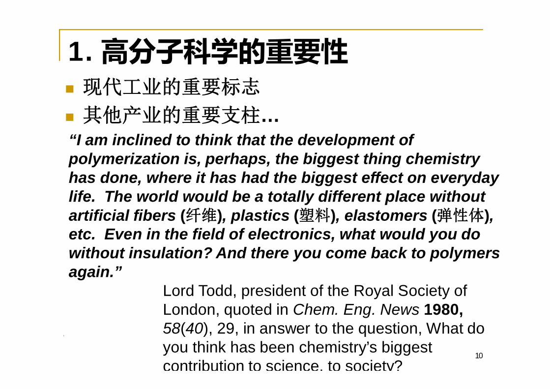
1.
…“I am inclined to think that the development ofpolymerization is, perhaps, the biggest thing chemistryhas done, where it has had the biggest effect on everydaylife. The world would be a totally different place withoutartificial fibers ( ), plastics ( ), elastomers ( ),etc. Even in the field of electronics, what would you dowithout insulation? And there you come back to polymersagain.”
Lord Todd, president of the Royal Society ofLondon, quoted in Chem. Eng. News 1980,58(40), 29, in answer to the question, What doyou think has been chemistry’s biggestcontribution to science, to society?
10

11
1.

——
12

13
0
2000
4000
6000
8000
10000
12000
14000
16000
18000
20000
1940 1960 1980 1998
2
1/7~1/8
20 20
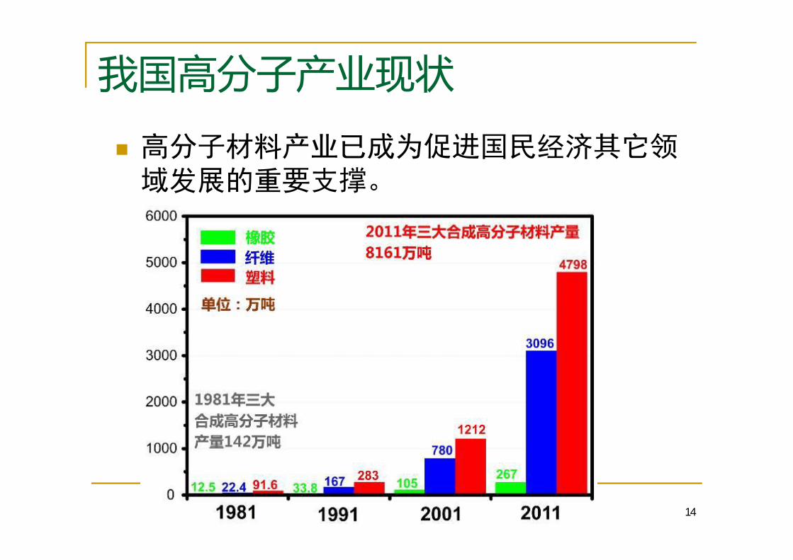
14

15
20118161 7400
40170
(PE PP PVC PS ABS)90%
160
200
400
600
800
1000
1200
1996 1997 1998 1999 2000 2001 2002 2003 2010 0
2 0 0
4 0 0
6 0 0
8 0 0
1 0 0 0
1 2 0 0
1 4 0 0
1 6 0 0
1 8 0 0
1 9 9 6 1 9 9 7 1 9 9 8 1 9 9 9 2 0 0 0 2 0 0 1 2 0 0 2 2 0 0 3 2 0 1 0
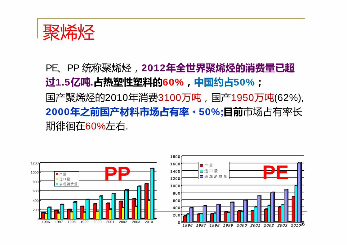
PE PP 20121.5 . 60% 50%
2010 3100 1950 (62%),2000 50%;
60% .
PP PE

17
604%
500
GDP 4%
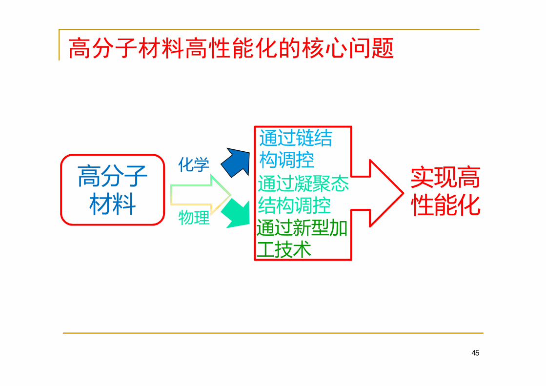
Why Polymers/Plastics?

18

Why Polymers/Plastics?
19

20
Carbon Fibers & Composite MaterialsPAN

Composite Materials in Commercial Aircrafts
21
20 30
C/C

Composite Materials in Fighters
22
60 80
40 60

Milestones of Polymer Materials
23
)
–
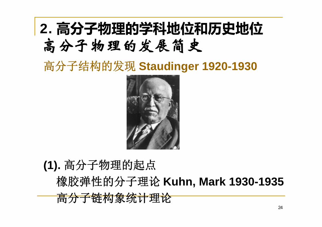
Staudinger 1920-1930
(1).Kuhn, Mark 1930-1935
24
2.

(2). DNA 1935-1965Flory Rouse-ZimmWatson-Crick d-Helix DNA, Natta
25
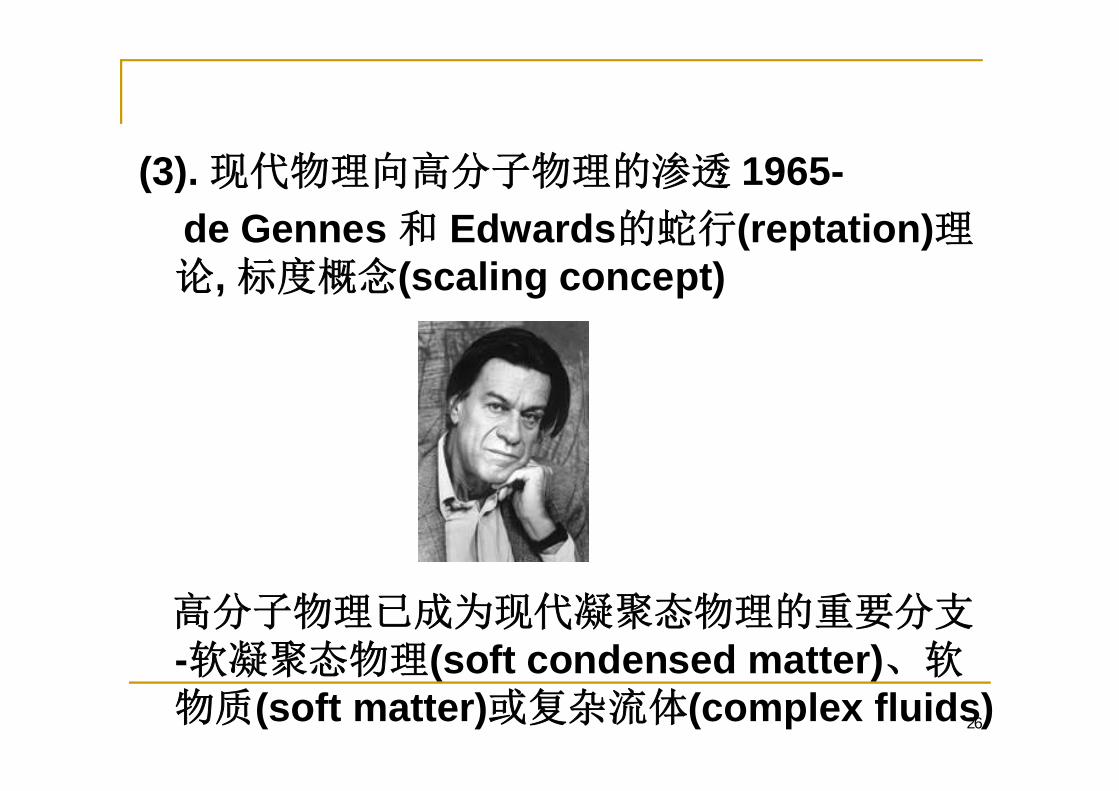
(3). 1965-de Gennes Edwards (reptation)
, (scaling concept)
- (soft condensed matter)(soft matter) (complex fluids)26
27
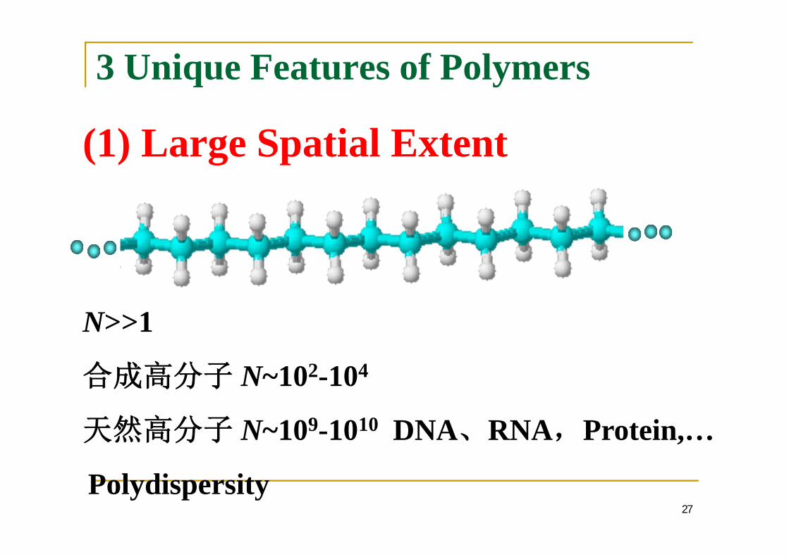
3 Unique Features of Polymers
N>>1
N~102-104
N~109-1010 DNA RNA Protein,…
(1) Large Spatial Extent
Polydispersity
28

The Mean Size of a Polymer Chain
29
~R h CN l
Freely Jointed Chainand Kuhn Segment le
2 2
0 0/ 6 / 6eR h L l
Unperturbed Chain:
=0.5 Ideal Chain Random Walk Chain=0.6 Real Chain Self-avoiding Chain
12 2 2
1 1
2N N
i ji j i
h Nl Nlr r
Root Mean Square of end-to-end Distance
L: Contour Length of a Chain
2 1/2h h N l
Radius of gyration

DNA, RNA & Virus
30
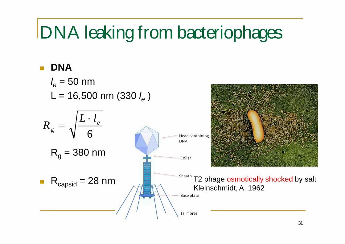
DNA leaking from bacteriophages
31
DNAle = 50 nmL = 16,500 nm (330 le )
Rg = 380 nm
Rcapsid = 28 nm
g 6eL lR
T2 phage osmotically shocked by saltKleinschmidt, A. 1962

DNA Condensation (DNA )
32

a. Tacticity –
b. Polymer Topology – Homo, Hetero, Copolymers
(2) Connectivity
33
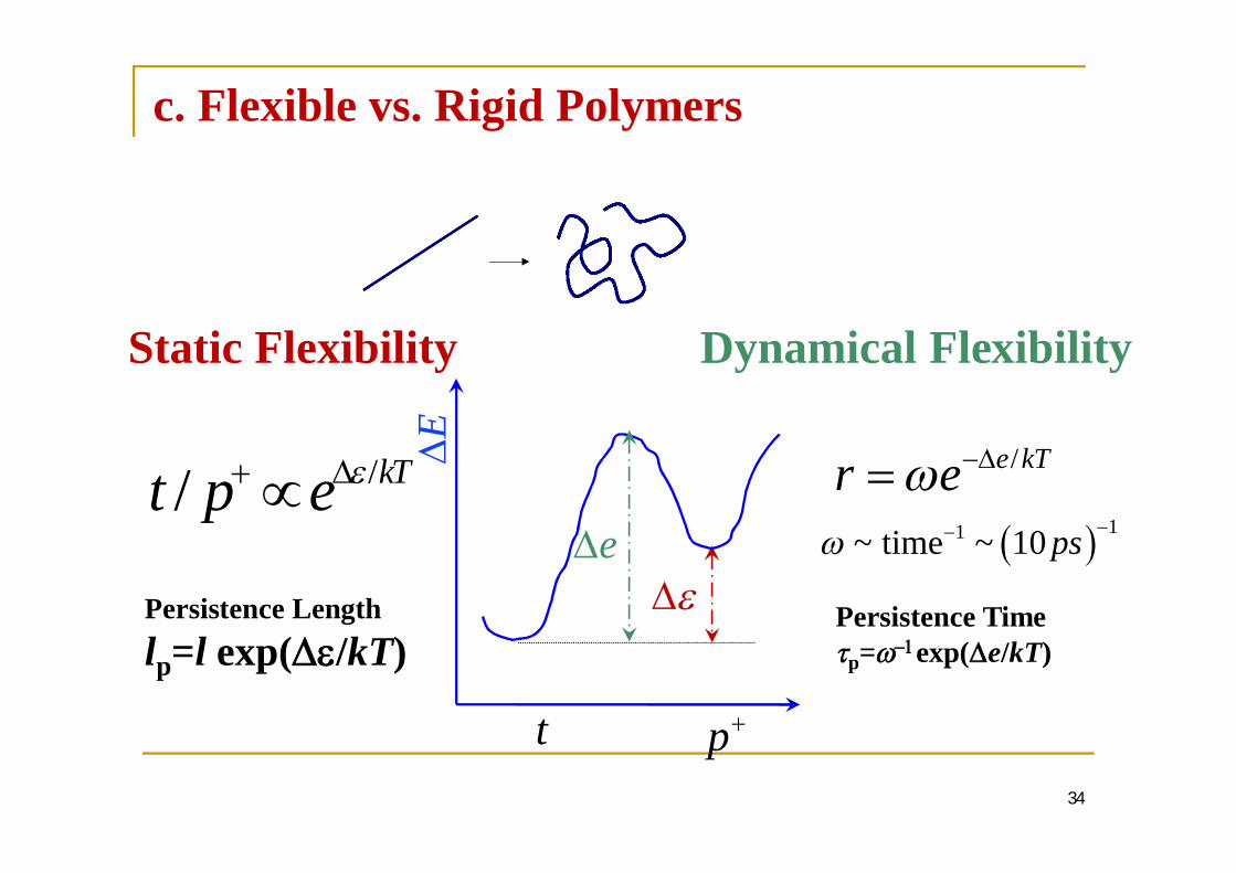
c. Flexible vs. Rigid Polymers
34
Static Flexibility
Persistence Lengthlp=l exp( /kT)
// kTt p e
Dynamical Flexibility
1
pt
e
E
Persistence Timep= exp( e/kT)
/e kTr e11~ time ~ 10 ps

d. Multiple Configurations(Confirmations)
35
lnS k4 N
ln / 'S k
Total number of chain conformations
Entropy of Chain Conformations
l
'The number of chain conformations in a state
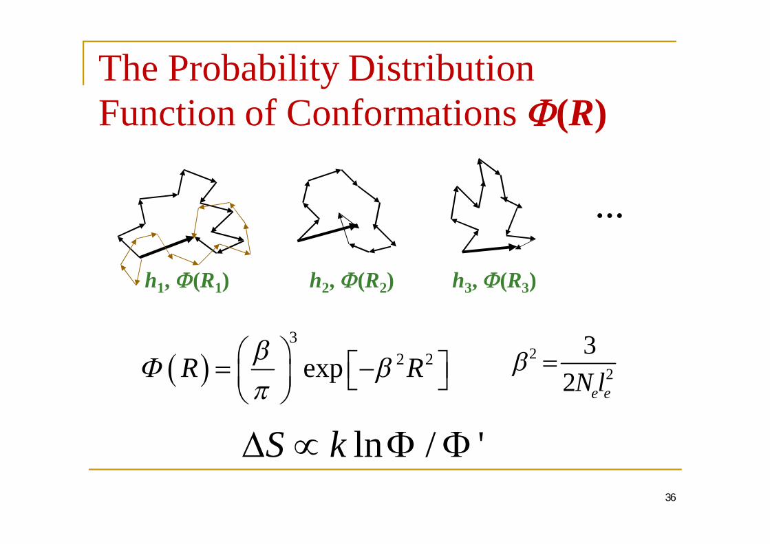
The Probability DistributionFunction of Conformations (R)
36
32 2expR R
h1, (R1)
…
h2, (R2) h3, (R3)
22
32 e eN l
ln / 'S k

(3) Multiple InteractionsVan der Waals, Hydrogen bond, Electrostatic
Multi-scale ….
37Glass, Gel
”

Condensed Matters
38Crystal Liquid Crystal
Blend
Triblock CopolymerHIPS & ABS Amorphous & Melt
39
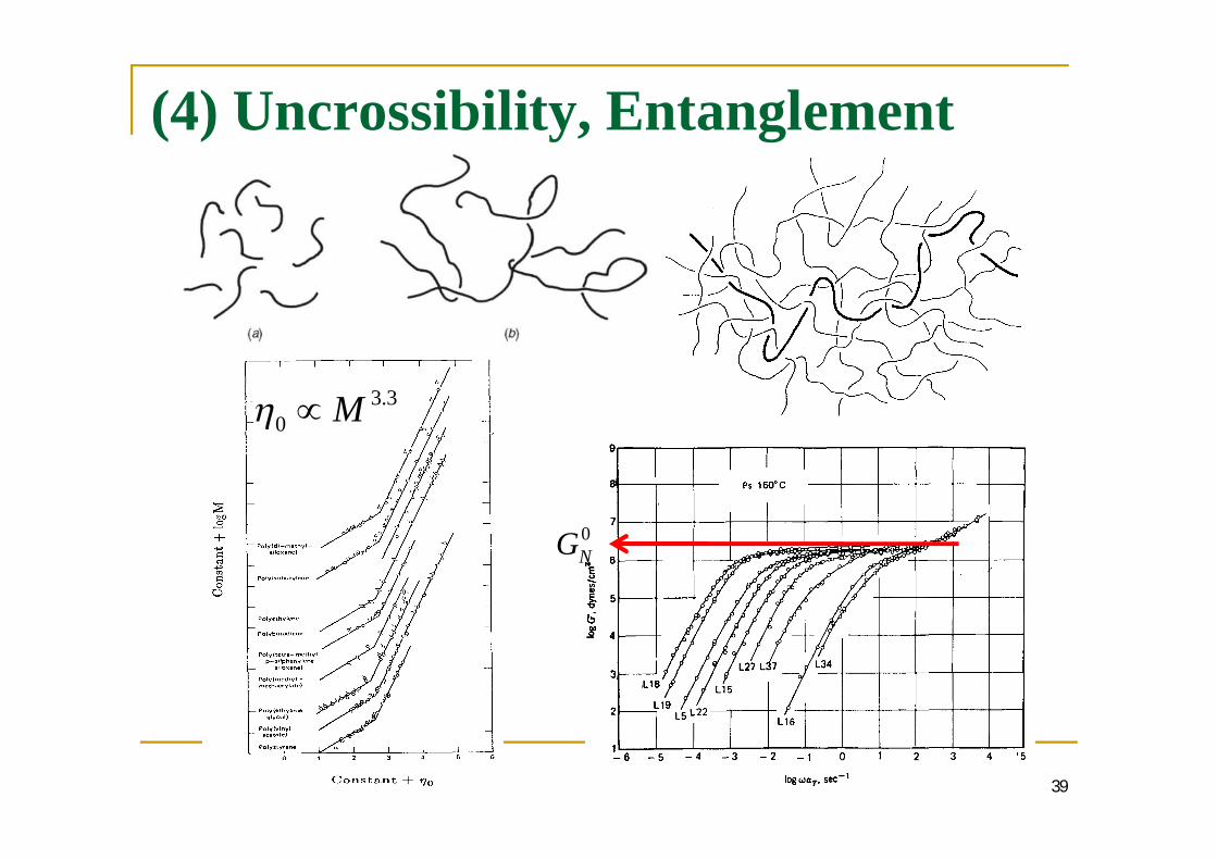
(4) Uncrossibility, Entanglement
3.30 M
0NG
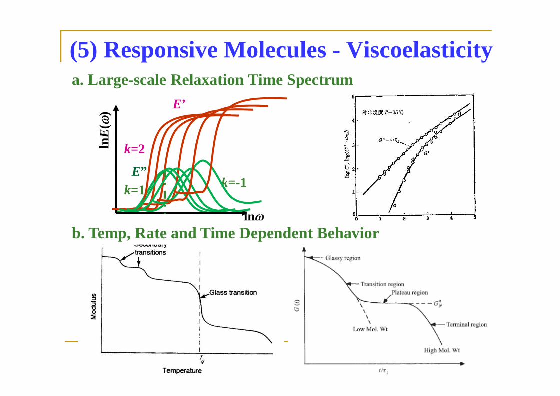
(5) Responsive Molecules - Viscoelasticity
40
a. Large-scale Relaxation Time Spectrumln
E(
)
ln
E’
k=2
k=1 k=-1E”
b. Temp, Rate and Time Dependent Behavior

b. Temp, Rate and Time Dependent BehaviorAn Example: Silly Putty
41
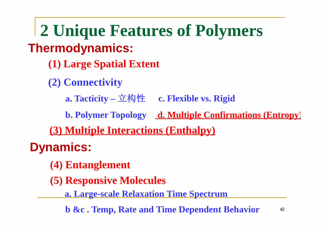
2 Unique Features of Polymers
42
(1) Large Spatial Extent
(2) Connectivitya. Tacticity –
b. Polymer Topology
c. Flexible vs. Rigid
d. Multiple Confirmations (Entropy)
(3) Multiple Interactions (Enthalpy)
(4) Entanglement
Thermodynamics:
Dynamics:
(5) Responsive Moleculesa. Large-scale Relaxation Time Spectrum
b &c . Temp, Rate and Time Dependent Behavior

43
Polymers are Complex yet Simple
Large number of degrees of freedomand multiple confirmations (Entropy)
Multiplicity of interactions (Enthalpy)
Allows averaging – Mean-field Theory
Universal properties – Scaling behavior
Osmotic, Viscosity, Viscoelasticity …

Shortcomings of Polymer Materials
Mechanical PropertiesModulus, Strength, Hardness, Creep, ……Surface PropertiesElectrical & Optical PropertiesAging & Stability……
44
Open Discussion
45

(1).
46

(2).
47

(3).
48
37%
21%
16%
1%
3%
13%
9%

(3).
49
(MPa) (g/cm3) (Mpa) (GPa) ( )iPP 230 0.94 244 4.1 0.9%
iPP 30-40 0.94 32-42 1.5-2 >50%400-800 7.8 51-102 ~200 ~100%
iPP

50

51
2 714 3
314 4782969 4.8 106
10 4.8 105 131050 (~3.8 )
52

53
(Monomer) (Segment) (Blob) (Chain)
( )
( )
( )
WLF Eq. Rouse-Zimm Model
Tube Model (entanglement & disentanglement time)
))
terminal relaxation timeMaster ( ) RelaxationSecondary ( ) Relaxation

( (4)) 2008( )
( , )Introduction to Polymer Physics (Oxford,1995, M. Doi)Polymer Chemistry (2nd, CRC Press, 2007, Hiemenz,P. C., Lodge, T. P.)Polymer Physics (Cambridge, 2003, Rubinstein)The Physics of Polymers (3nd) (Springer, 2007, G. R.Strobl)Introduction to Physical Polymer Science (Wiley,2006, L. Sperling)Principles of Polymer Chemistry (Flory)
( Mark, Tobolsky et. al.)
54
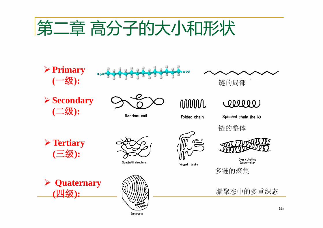
Primary( ):
Secondary( ):
Tertiary( ):
Quaternary( ):
55

2.1 (local)
2.1.1 (Constitutions or Architectures)
-CH2-CH2-
2.2.1.1
2.2.1.2
56

57
2.2.1.3
Branched polymer Cross-linked polymer

58
Star ( ) polymers
homo-armed( )
hetro-armed( )
Hyperbranched ( ) Polymersand Dendrimers ( ):
The composition of dendrimerscan be varied throughout themolecule in a systematic way
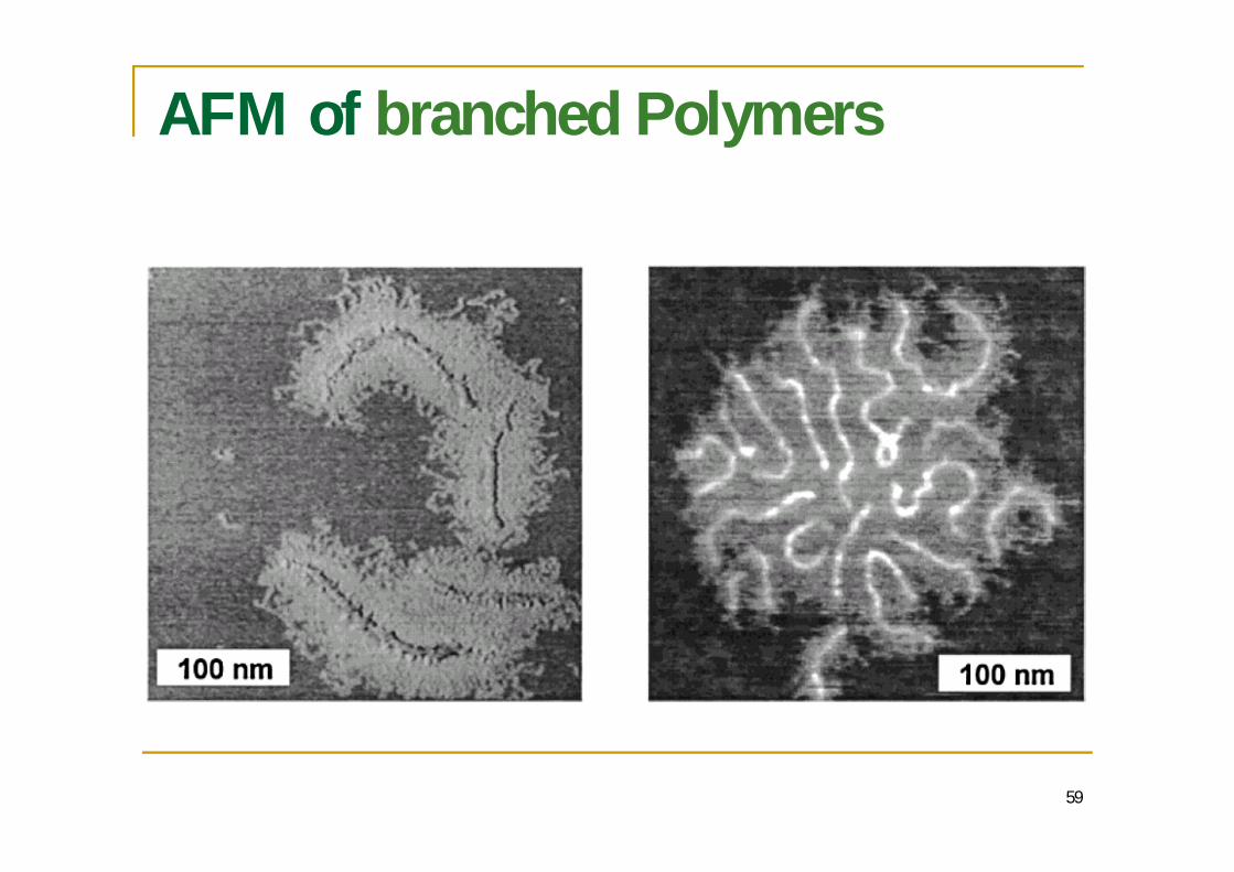
AFM of branched Polymers
59

2.1.1.4
Homopolymers ( ):
Linear polymer
Branched polymer
Copolymers ( ):
Linear random copolymer
Linear alternating copolymer
Linear block copolymer
Graft copolymer
: two different monomersand
60
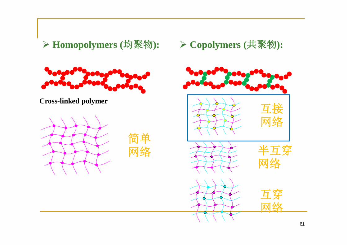
61
Cross-linked polymer
Homopolymers ( ): Copolymers ( ):

2.1.2 (Configurations)
Arrangements fixed by the chemical bonding in themolecule, such as cis ( ) and trans ( ), isotactic( ) and syndiotactic ( ) isomers. Theconfiguration of a polymer cannot be altered unlesschemical bonds are broken and reformed.
62
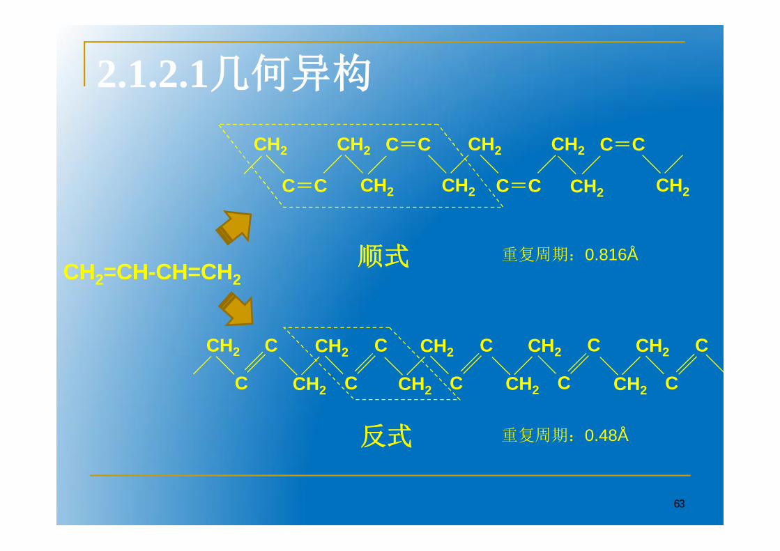
2.1.2.1
63
CH2 CH2
C C CH2CH2
C C
CH2
CH2 CH2
C C
C C
CH2
0.816ÅCH2=CH-CH=CH2
CH2
CH2C
C CH2
C
C
CH2
CH2
C
C
CH2
CH2
C
C
CH2
CH2
C
C
0.48Å

2.1.2.2
: C*?? 64
C*
COOH
OHCH3
H
*C
COOH
HOCH3
H

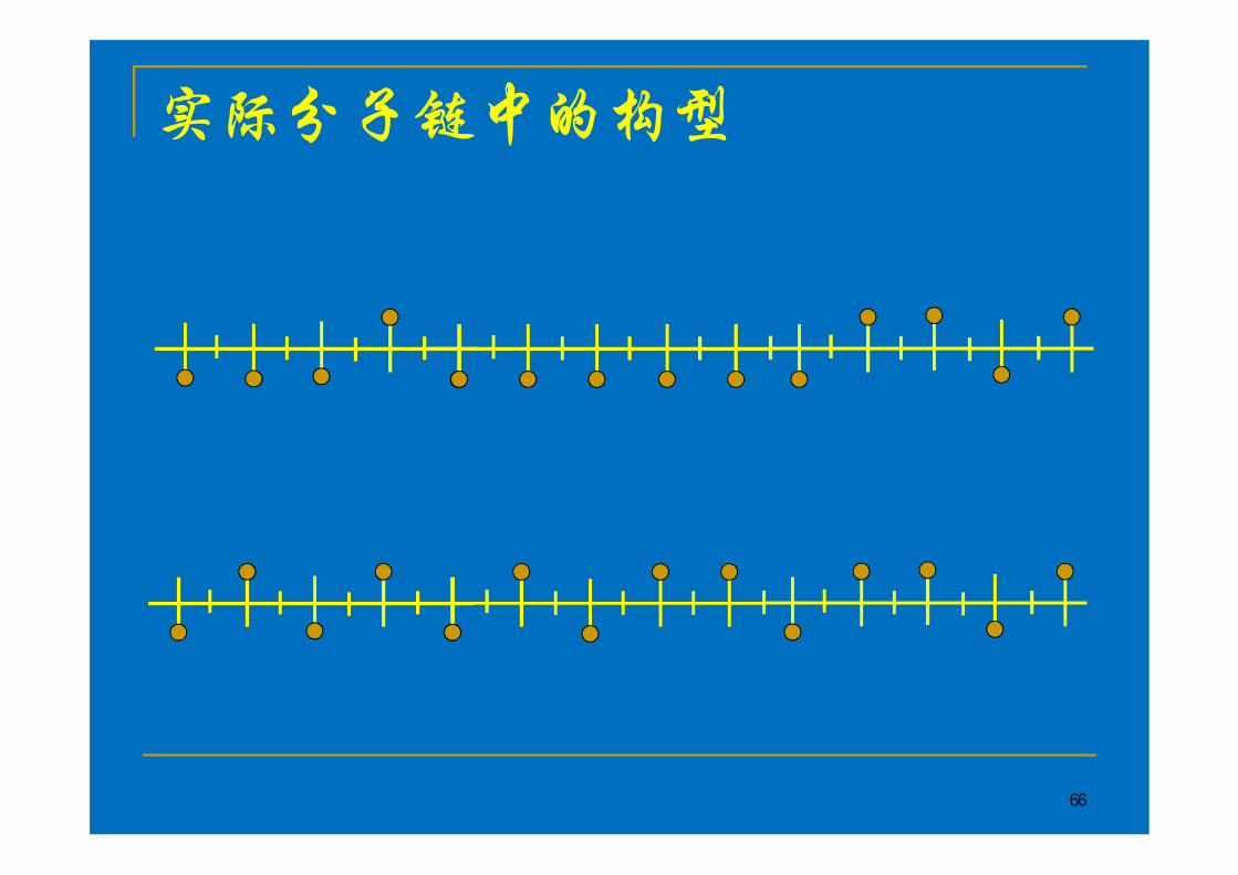
isotactic
syndiotactic
atactic
66

67
(diads) (triads)
, mm
, rr
, mr
m
r
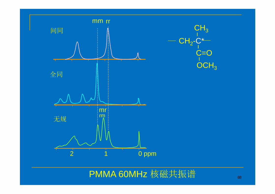
68PMMA 60MHz
CH2-C*CH3
C=OOCH3
2 1 0 ppm
mm rr
mrrm
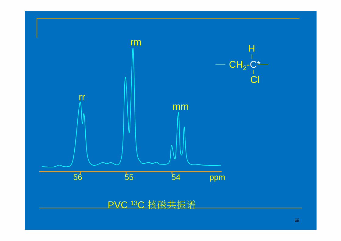
69
CH2-C*H
Cl
mm
rm
rr
56 55 54 ppm
PVC 13C

70
(tetrads)
mmm
mmr
rmrrrr
rrm
mrm

71
(pentads)mmmm
rmrr
rmrm
mmrr
mmrmrmmr
mmmr
rrrr
rrrm
mrrm
( )
( )
( )

Hotta, H., et al., PNAS, 103(42), 15327 (2006)
72

73
PP-RHIPP
PE
….

74
75

76

77
( )
()
( )

BOPP
78

79
BOPP
BOPP BOPP1999
973 3010
PE

2:
80
(TM)(ET)
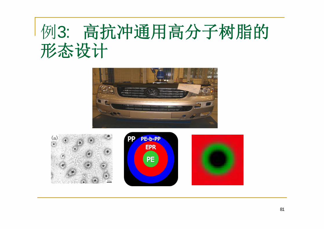
3:
81

-PAN
82

83
PAN
ITA( )
ITA
ITA
AN!

2.1.2 (Configurations)
,
!!!
84

2.2 (glouble)
85
Molecular Weight (MW) and Molecular Weight Distribution(MWD) Degree of polymerization (DP)
~R h N l= 0.6 0.5
2.2
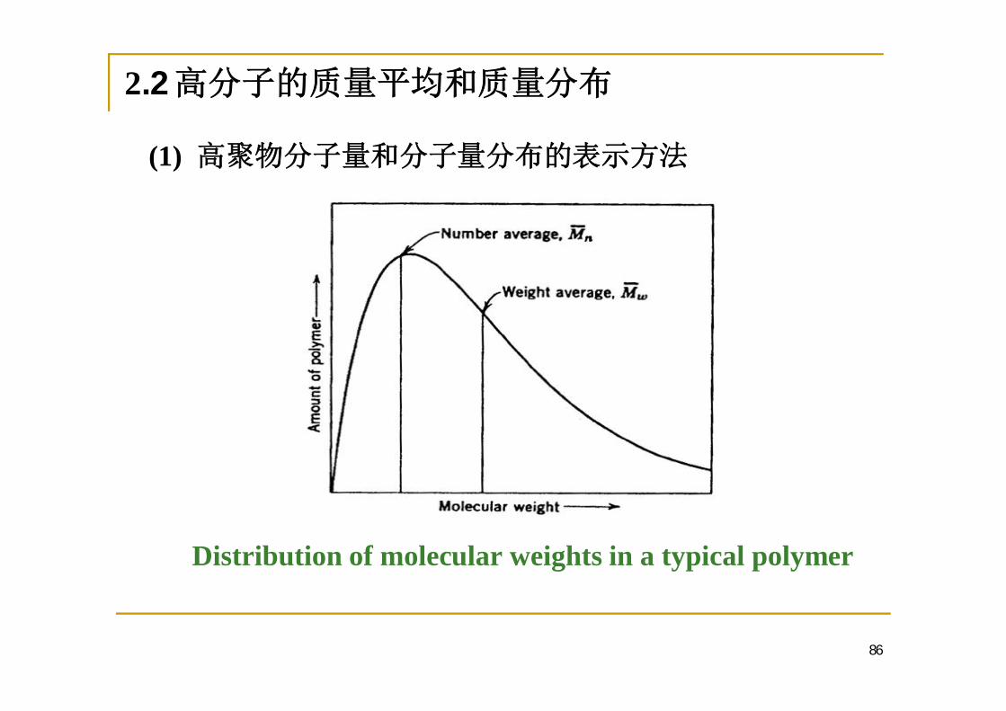
86
(1)
Distribution of molecular weights in a typical polymer

87
5g 4 8g 5 10g 3?
: 12 ; : 90g ii
ii
nNn
4/12
5/12
3/12
ii
ii
wWw
4 5/90
5 8/90
3 10/907.5n i i
iM N M 8w i i
iM W M
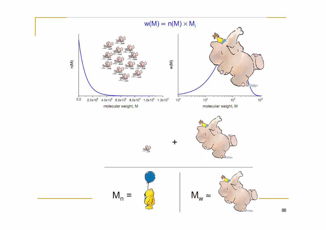
88

89
Definitions of Average MWs and MW Distribution
ii
n n ii
n Nn
1ii
Ni
iw w ii
w Ww
1ii
W
n: total mole number; ni: molenumber of ith molecule with molemass of Mi; Ni: mole fraction ofith molecule;
(1) Number-average molecularweight ( ):
(2) Weight-average molecularweight ( ):
nMnw ii
iw
ii
MwM
w
ii iw n M ii
in w
M
=dd
=d
>
w: total weight of the sample; wi:weight of the ith molecule; Wi: weightfraction of ith molecule.
=1
d =d
d
=
= / d = 1= 1
=
= /
ii iW N M ii
iN W
M
= = = = =

90
(3) Z-average molecular weight(Z ):
(4) Viscosity-average molecularweight ( ):
3
2
2i
i
ii ii
zi
i
ii
i
i
i ii
i
i
w M
w
z MM
z
n M
n MM
1 1// 1i i
i i
i iii
i i
i
nw M
w
M
nM
M
wz nM MM M
=
=
=d
d
=
: Mark-Houwink =kMK-M-

MW Distribution & Polydispersity( )
91
Schulz
Tung
Logarithm normaldistribution
2 2( )n n nM M
2d
dw
M MN M
N MM
M M
22 1wn
nn M
MM
w
n
MdM
Width of molecular weight distribution ( ):
Polydispersity ( ):
MW Distribution Function/,
/
,
i i i i
i i ii i
i i i i
i i ii i
n n w MN Mn n w M
w w n MW Mw w n M
=d
d=
= ( ) =

Bimodal Distribution
92
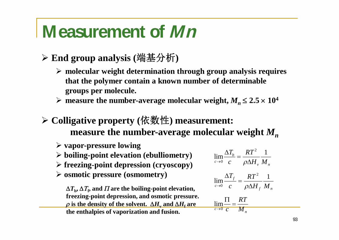
Measurement of Mn
93
End group analysis ( )molecular weight determination through group analysis requiresthat the polymer contain a known number of determinablegroups per molecule.measure the number-average molecular weight, Mn 2.5 104
Colligative property ( ) measurement:measure the number-average molecular weight Mn
vapor-pressure lowingboiling-point elevation (ebulliometry)freezing-point depression (cryoscopy)osmotic pressure (osmometry)
Tb, f, and are the boiling-point elevation,freezing-point depression, and osmotic pressure.
is the density of the solvent. Hv and Hf arethe enthalpies of vaporization and fusion.
nv
bc MH
RTcT 1lim
2
0
nf
f
c MHRT
cT 1lim
2
0
nc M
RTc0
lim

94
Vapor-phase osmometry (VPO, )
Small temperature difference resulting fromdifferent rates of solvent evaporation from andcondensation onto droplets of pure solvent andpolymer solution maintained in an atmosphereof solvent vapor.Measure Mn that is too lower for membraneosmometry method.Calibrated with low-molecular weightstandards: a relative method.Quasi-steady-state phenomena. care must betaken to standarize such variables as time ofmeasurement and drop size betweencalibration and sample measurement.
11
22
1
2
21
2
//MwMwA
nnA
nnnAT
Measurement chamber of VPO(Pasternak, 1962). Droplets of solventand polymer solution are placed, withthe aid of hypodemic syringer, on the“beads” of two theristors used astemperature-sensing elements andmaintained in equilibrium with anatmosphere of solvent vapor.

95
Membrane osmometry ( )
0cc Van’t Hoff relation
Polymer solution pure solvent
P P2 , , 0, ,s sP T P T
1
1 0cV c2
2 30
1c
RT A c A cM
RTM

96
Based on the Flory-Huggins Theory of Polymer Solutions
21 1
2
2
1 1 12
1
cRTc V c M
T cA
V
RM
22 2
1
12V
Asecond Virialcoefficent
11
mixFn
Chemical potentialof solvents
Flory-Hugginsparameter
0 0ic ci
i
i i
cRTM
i
i i
ii
cMRTcc
ii
i ii
nRTc
n M
1
n
RTcM
97
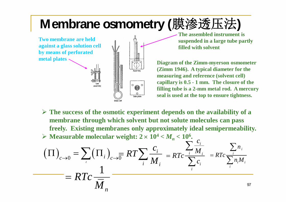
Membrane osmometry ( )
Diagram of the Zimm-myerson osmometer(Zimm 1946). A typical diameter for themeasuring and reference (solvent cell)capillary is 0.5 - 1 mm. The closure of thefilling tube is a 2-mm metal rod. A mercuryseal is used at the top to ensure tightness.
Two membrane are heldagainst a glass solution cellby means of perforatedmetal plates
The assembled instrument issuspended in a large tube partlyfilled with solvent
The success of the osmotic experiment depends on the availability of amembrane through which solvent but not solute molecules can passfreely. Existing membranes only approximately ideal semipermeability.Measurable molecular weight: 2 104 < Mn < 106.
0 0ic ci
i
i i
cRTM
i
i i
ii
cMRTcc
ii
i ii
nRTc
n M
1
n
RTcM

Measurement of Mw – light scattering
98
General set-up of a light scattering ( ) experiment
Incident beamIntensity I0
Scattered beamIntensity I(q)
Detector
Sample
if kkq 2if kk
4 sin2
q
Scattering vector ( ):
where
: wavelength of the radiation
Tyndall ( ) phenomenon

Theory of Light Scattering
The intensity Is of the wave scattered by a single molecule:
42
4 2
16iI cN I
M r
Rayleigh ( )derived:
iI
sI
: polarizability ( )
The averaged intensity I of the wave scattered by many molecules:
42
4 2
16isI I
r

100
The change in the square of the refractive index ( ) n is linear
2 20 4 cNn n
M 2n M dn
N dc4
24 2
16iI cN I
M r
22 2
4 24
in dn
r dcMIN
c I
Rayleigh ratio( )
2
i
r KcMI
R I 22 2
4
4 n dnKN dc
i ii
i i i wi i i
i
c MR R K c M Kc KcM
c
Hence, dilute scattering measurementsgive the weight-average molar mass of apolydisperse polymer sample.
1
w
KcR M

101
For small particles d< /20The contrast required for scattering from polymer solutionsprimarily comes from concentration fluctuations
22
2
12
mix mixmix mix
F FF F
1 1
22
2
1 ...2
mix mix
mix
F F F n
F
122
2mixFI kT
c
2I
F kT
1 1mixF
n
Based on the Flory-Huggins Theory of Polymer Solutions:I c
2I c
102
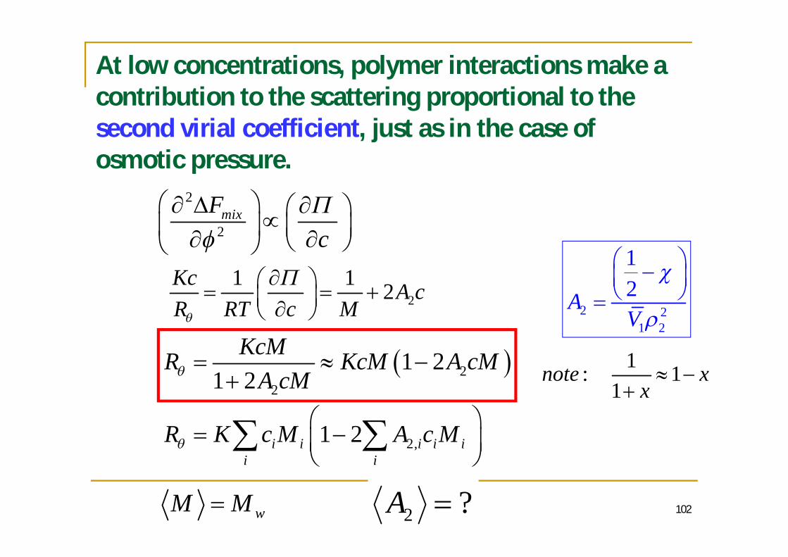
21 1 2Kc A c
R RT c M 2 21 2
12AV
22
1 21 2
KcMR KcM A cMA cM
2 ?AwM M
2,1 2i i i i ii i
R K c M A c M
At low concentrations, polymer interactions make acontribution to the scattering proportional to thesecond virial coefficient, just as in the case ofosmotic pressure.
2
2mixF
c
1: 11
note xx
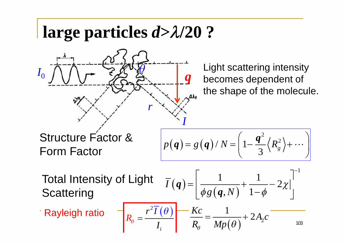
large particles d> /20 ?
103
11 1 2
, 1I
g Nq
q
21 2Kc A c
R Mp
2
i
rI
RI
r
I0
I
q
22/ 1
3 gp g N Rqq qStructure Factor &Form Factor
Light scattering intensitybecomes dependent ofthe shape of the molecule.
Total Intensity of LightScatteringRayleigh ratio

104
11 1 2I
Npq
q
22
21 1 2
3gRKc A c
R Mq
00
1 11 x
xx 2
221 2
3gRKc cY A c
R Mq
' 1 1 2K c cR Np q
22 1
,c MNV
2 21 2
12AV
21 2Kc A c
R Mp q
2 22
22
1 81 sin 29 2
h A cM
4 sin2
q
221
3 gp Rqq
22
6ghR

Measurement of M
105
dd
F vA y
/ /dv dy d dt
For Newtonian fluids
1-dimension
: Stress( ): Viscosity( )
:Velocity Gradientdd
vy/d dt :Flow Rate
=

106
Nomenclature of solution viscosity
r: ( ); sp: ( ); red: ( );inh: ( ); [ : ( )
: viscosity of polymer solution at temperature T
0: viscosity of pure solvent at T.

Theoretical and Experimental basis
107
[ ] aKMMark-Houwink equation:
Flory-Fox equation3/22
g hR VM M
2 2gR M 3 1M
Experiments:
Theory
Size of the polymer chain :
empirical formula
Solution viscosity as a measure of polymer molecular weight

108
Viscosity measurement
The small molecular liquids and dilutepolymer solutions are Newtonian flow:the viscosity does not change with theshear stress and shear rateMeasurements of solution viscosity areusually made by comparing the effuxtime t ( ) required for a specifiedvolume of polymer solution to flowthrough a capillary ( ) tube withthe corresponding effux time t0 of thepure solvent.
tBAt
ltVm
lVtghR
88
4
000 //
tBAttBAt
r
0tt
r0
01t
ttrsp
If B/t is much small than At and0

109
Treatment of viscosity data
aKM][
ckcsp 2'
...32
1lnln32spsp
spspr
232 '31
21'ln ckck
cr
ckc
r 2"ln
Huggins equation:
If sp < 1, r can be expressed byTaylor series expansion
Mark-Houwink equation:
Viscosity-average molecular weight( ):
= == = =

Measurement of MWD
110
Gel permeation chromatography ( )Size exclusion ( ) chromatography

111
High MW
Elution volume
Am
ount
ofpo
lym
erel
uted Mark of
injection
Low MWGPC curve:
ebVaMlogVe: elution volume
Samplemixture
Separation
begins
Partialseparation
separation
complete
separatedsamples
leave column
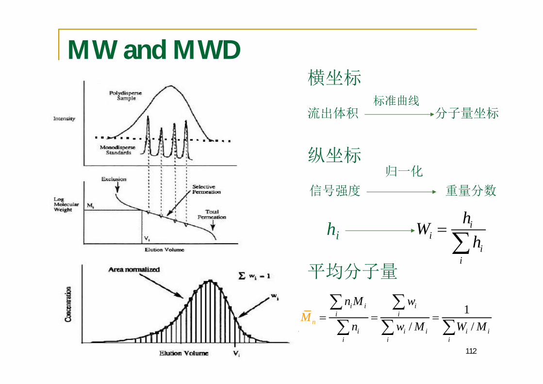
112
MW and MWD
ii
ii
hWh
hi
1/ /
i i ii i
i i i ii i
ni
i
n M w
n w MM
W M

113
Universal calibration ( )log A A
A eM A B V3/22
~ ~g hR VM M
,hA hB A BA BV V M M
Universal calibration parameter
1 1log log log1 11 1log log1 1
11
1 1 log1 1
A AB A
B B B
A AA AB e
B B B
AAe
B
Be
AA A
B B B
B
a K
a KM Ma a Ka KM A B Va a K
a BAa a K
A
Va
B V
,A Ba aA A B BA B
K M K M
log B BB eM A B V
Flory-Fox equation
Mark-Houwink equation

2.2.2
trans ( ) and gauche ( ) conformations:Potential energies associatedwith the rotation of centralC-C-bond for ethane (dashedline) and butane (solid line).The sketches show the twomolecules in views along theC-C-bond.
Rotational Isomeric States ( RIS)
2 2N
114

Random coil ( ) of polymer
i-1i+1
i
In melt or solution
: ( )
Zigzag conformation of PE (21 helix) Random coil
ComputerSimulation of aSingle Chain inSolutions
115

(zigzag) ( )
Polyproplenes in Crystals
116

2.2.3 (flexibility)
2.2.3.12.2.3.1 Static Flexibility
1 ( )
lp=l exp( /kT)
117
/kTp e
pt
// kTt p e
lp l

2.2.3 (flexibility)2.2.3.2 Dynamical Flexibility
1
2t ( )
p= exp( E/kT)
E p
2.2.3.3
118
/E kTr e 11~ time ~ 10 ps
t p+
pt

2.2.4
2.2.4.1
<h2>
<Rg2>
119
)
L=Nl ??
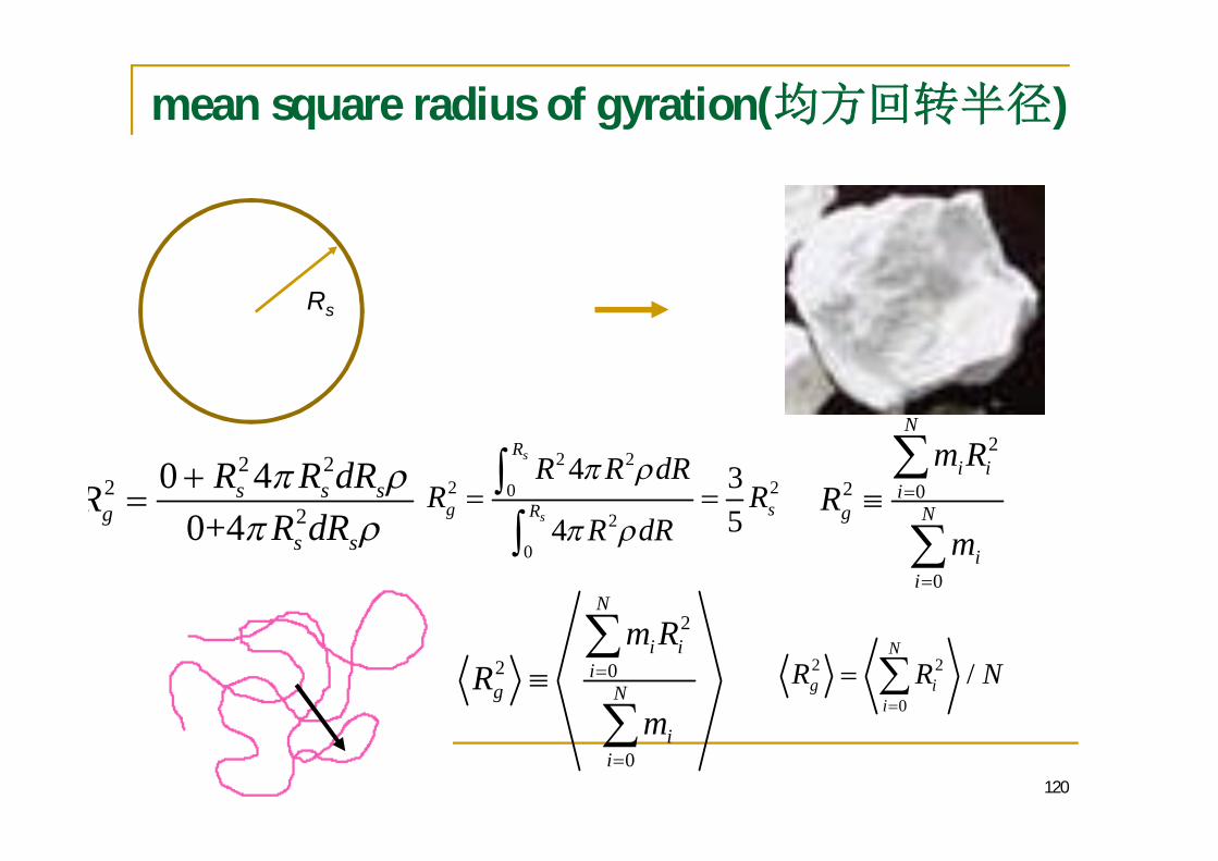
mean square radius of gyration( )
120
Rs
2 22
20 4
0+4s s s
gs s
R R dRRR dR
2
2 0
0
N
i ii
g N
ii
m RR
m
2 2
0/
N
g ii
R R N
2 22 20
2
0
4 354
s
s
R
g sR
R R dRR R
R dR
2
2 0
0
N
i ii
g N
ii
m RR
m
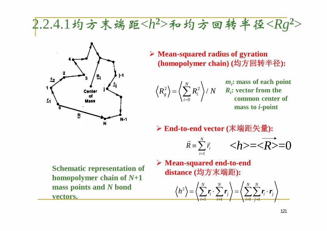
2.2.4.1 <h2> <Rg2>
Schematic representation ofhomopolymer chain of N+1mass points and N bondvectors.
N
iirR
1
2
1 1 1 1
N N N N
i j i ji i i j
h r r r r
End-to-end vector ( ):
Mean-squared end-to-enddistance ( ):
Mean-squared radius of gyration(homopolymer chain) ( ):
2 2
0/
N
g ii
R R Nmi: mass of each pointRi: vector from the
common center ofmass to i-point
<h>=<R>=0
121

122
<h2>
l: the bond lengthei: the unit vector
(1)
(2)
N n!!!
1 2 3 1... N Nh r r r r r 2h
i ilr e
2h
cosi j ije e1
2 2 2
1 12 cos
N N
iji j i
h Nl l
N=2n-1 2n
= = + 2
= + 2 = + 2

(1) (freely-jointed) <h2>
12 2 2
fj1 1
2 cosN N
2ij
i j i
h Nl l Nl
h2fj N
ij ~ 0-180 cos 0ij
123
Nn!!!
N=2n-1 2n
< >=< > / ? ? ?
??
??
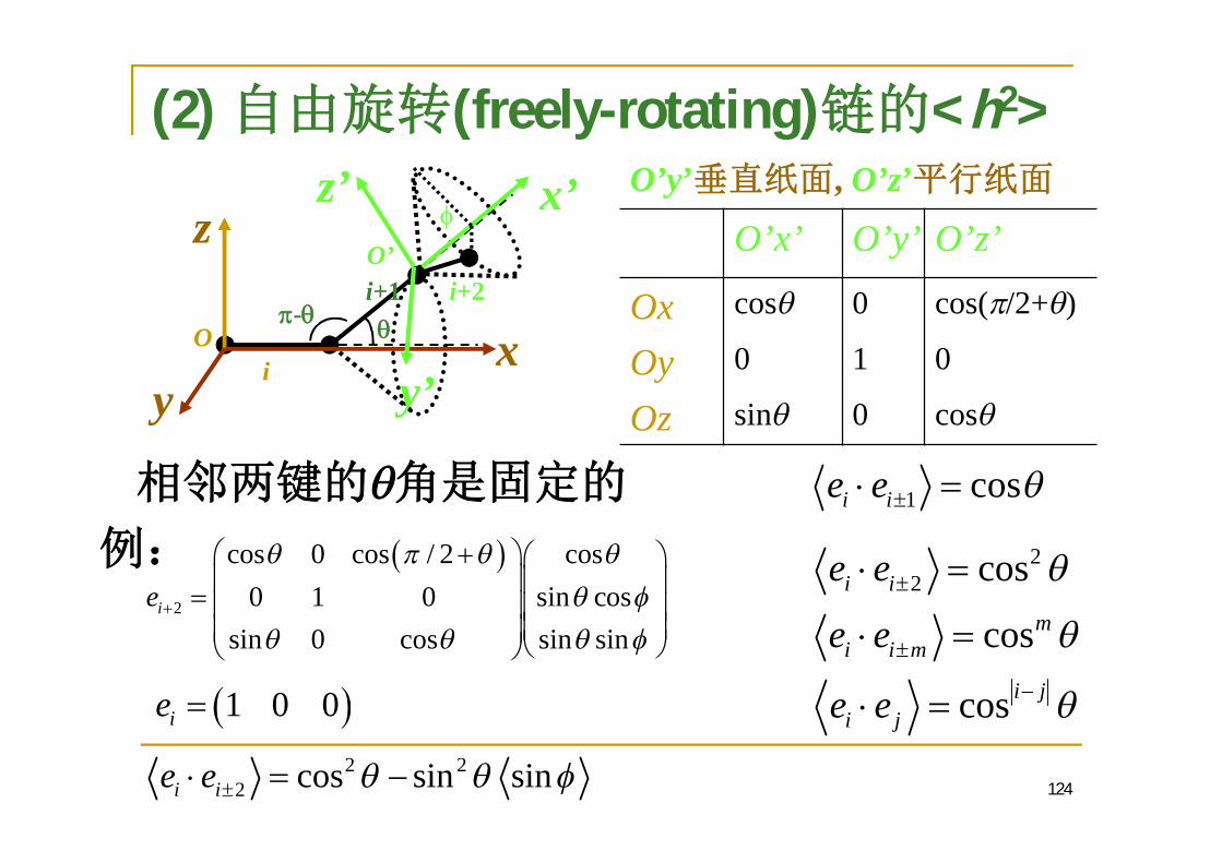
(2) (freely-rotating) <h2>
22 cos
cos
cos
i i
mi i m
i ji j
e e
e e
e e
2
cos 0 cos / 2 cos0 1 0 sin cos
sin 0 cos sin sinie
2 22 cos sin sini ie e
O’x’ O’y’ O’z’
Ox cos 0 cos( /2+ )
Oy 0 1 0
Oz sin 0 cos
O’y’ , O’z’
1 cosi ie e
-
i
i+1 i+2
xy
zx’
y’
z’
1 0 0ie
O
O’
124
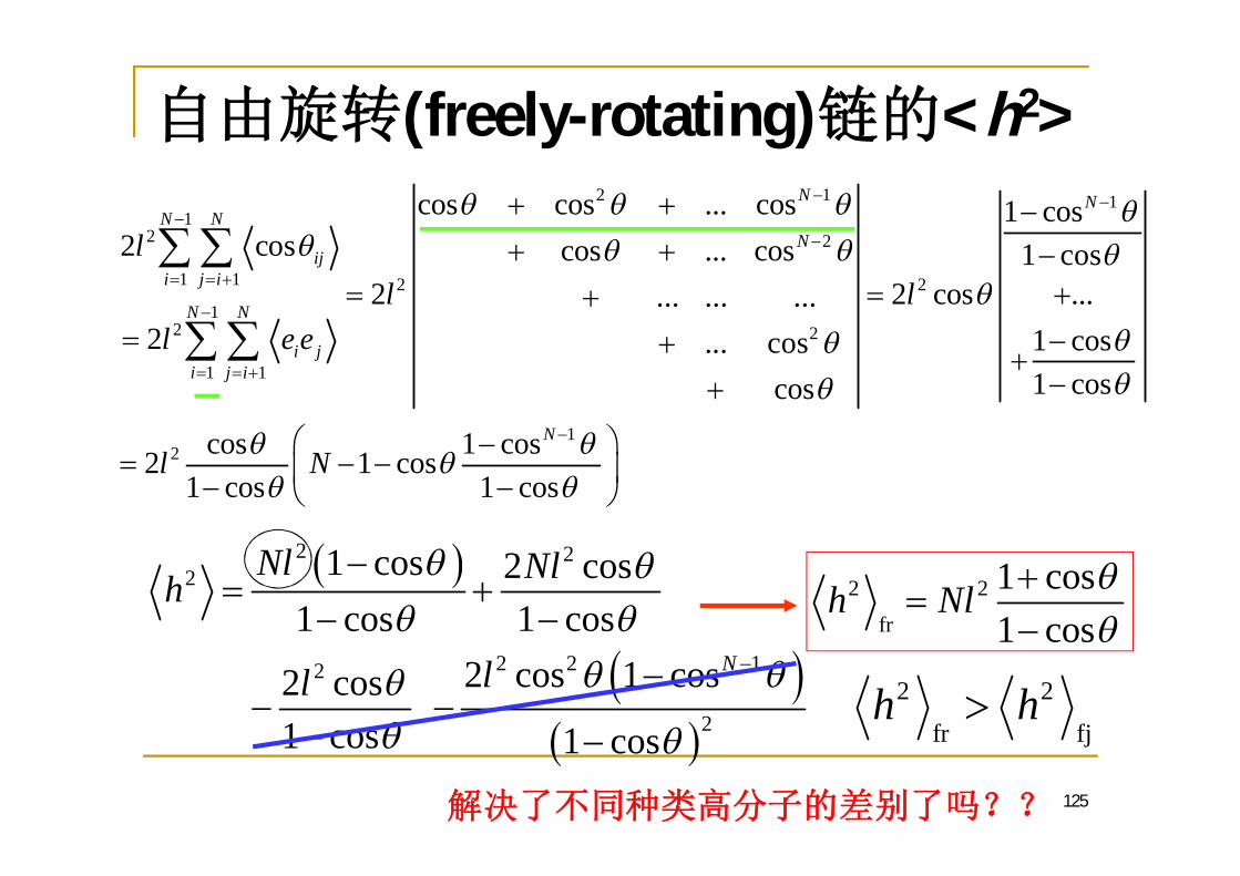
(freely-rotating) <h2>2 1 1
12 2
1 1 2 21
2 2
1 1
12
cos cos ... cos 1 cos2 cos cos ... cos 1 cos
2 2 cos ...... ... ...2 1 cos... cos
1 coscos
cos 1 cos2 1 cos1 cos 1 cos
N NN N
Nij
i j i
N N
i ji j i
N
ll l
l e e
l N
2 22
2 2 12
2
1 cos 2 cos1 cos 1 cos
2 cos 1 cos2 cos1 cos 1 cos
N
Nl Nlh
ll
2 2
fr
1 cos1 cos
h Nl
j
2
fr
2
fh h
125
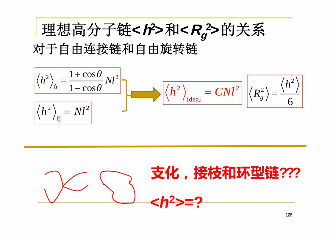
<h2> <Rg2>
22
6g
hR
126
2 2fr
1 cos1 cos
h Nl
2 2
fjh Nl
2 2ideal
h CNl
???
<h2>=?

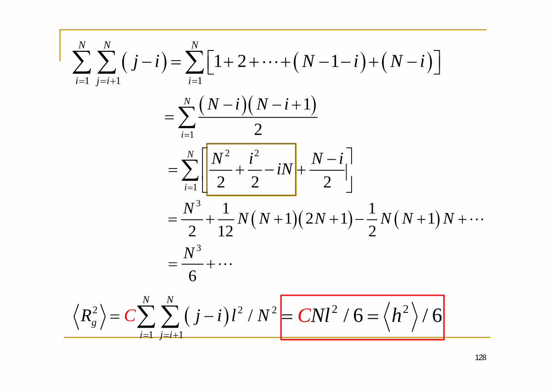
Radius of gyration
127
2
1 1 1 1
12
N N N N
ij ij iji j i i j
r r r
jij iR Rr
2 2
1 1 1 1 1 1
1 1 1 22 2 2
N N N N N N
ij ij j i j i i j i ji j i j i j
r r R R R R R R R R
2 2
1/
N
i gi
N RR 2 2 2
1 1
N N
j gi j
N RR0 0 0 0
0n n n n
i j i ji j i j
R R R R
2 2 2
1 1/
N N
g iji j i
R Nr
rij i j
Ri im
rij =hij: i j
2 2ij Ch j i l
Ri
Rj
rij
m
2 2
1 1/
N N
iji j i
h N 2 2
1 1
/N N
i j i
l NC j i
2 2 2
1 1
N N
ij gi j i
N Rr
=1 + cos1 cos
= 1 or
2 2 2
0 0 0/ /
N N N
g i i i ii i i
R m R m R N
128
1 1 11 2 1
N N N
i j i ij i N i N i
1
12
N
i
N i N i
2 2
1 2 2 2
N
i
N i N iiN
3 1 11 2 1 12 12 2
N N N N N N N
3
6N
2 2 2
1 1/
N N
gi j i
R NC j i l 2 2/ 6 / 6Nl hC

??
1.
2.129
2 6/5h N
2h N
(2)(1)

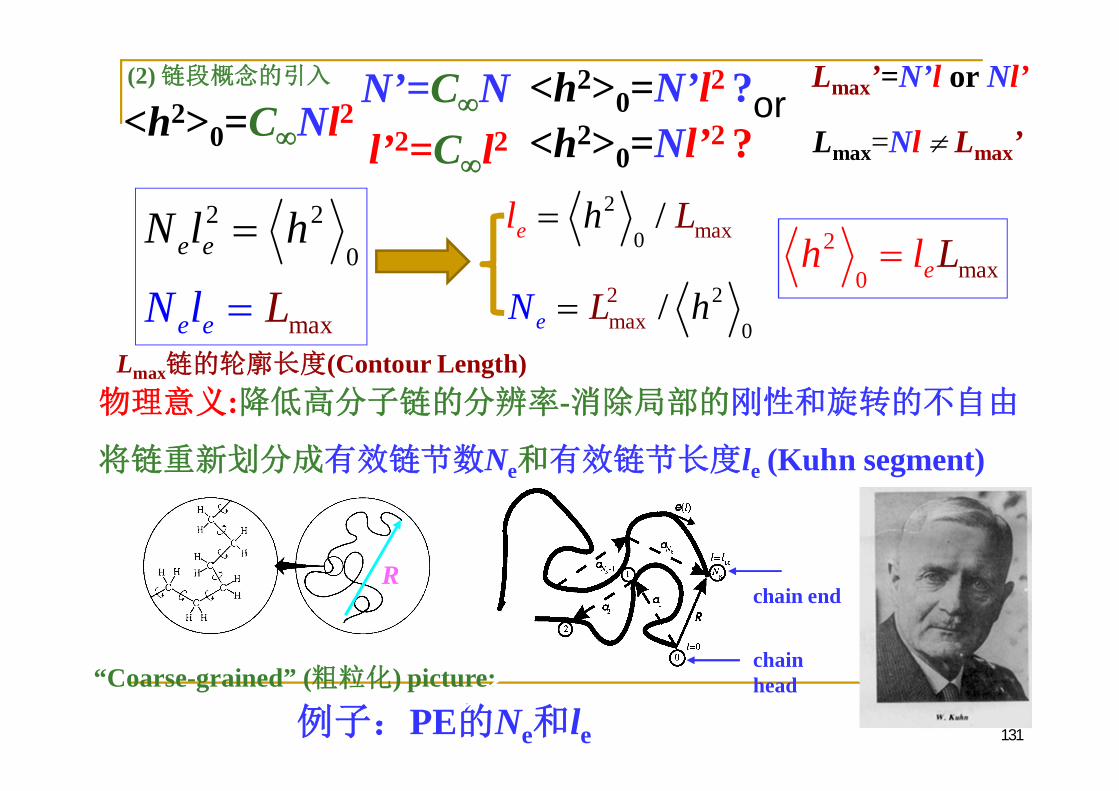
When does the freely jointed chain works& Kuhn segment le
(1)
130
<h2>0=C Nl2<h2>~N6/5
C
- > -- << -
131
“Coarse-grained” ( ) picture:
R
: -
Ne le (Kuhn segment)
chainhead
chain end
PE Ne le
max
2 20e
e
e
eN l
N l
L
h
Lmax (Contour Length)
m2
0 axeLh l
<h2>0=C Nl2N’=C Nl’2=C l2
<h2>0=N’l2 ?<h2>0=Nl’2 ?
orLmax=Nl Lmax’
2max
2
0/e LN h
2
0 max/e h Ll
Lmax’=N’l or Nl’(2)
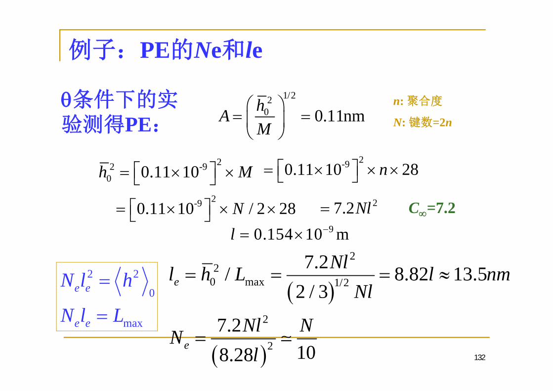
PE Ne le
PE1/22
0 0.11nmhAM
22 -90 0.11 10h M
2 2
0
max
e e
e e
N l h
N l L
22
0 max 1/2
2
2
7.2/ 8.82 13.52 / 3
7.2108.28
e
e
Nll h L l nmNl
Nl NNl
n:
N: =2n
132
2-90.11 10 28n2-90.11 10 / 2 28N
90.154 10 ml
27.2Nl C =7.2
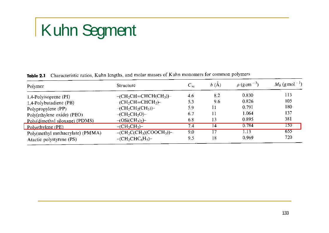
Kuhn Segment
133

(2) C2 2 2 2
0 fj 0/ /h h h NlC
(3)1/ 21/ 2
2 2 2 2
0 fr 0
1 cos/ /1 cos
h h h Nl
(1) A1/ 2
2
0/ MA h
(4) le2
max0e /l h L134
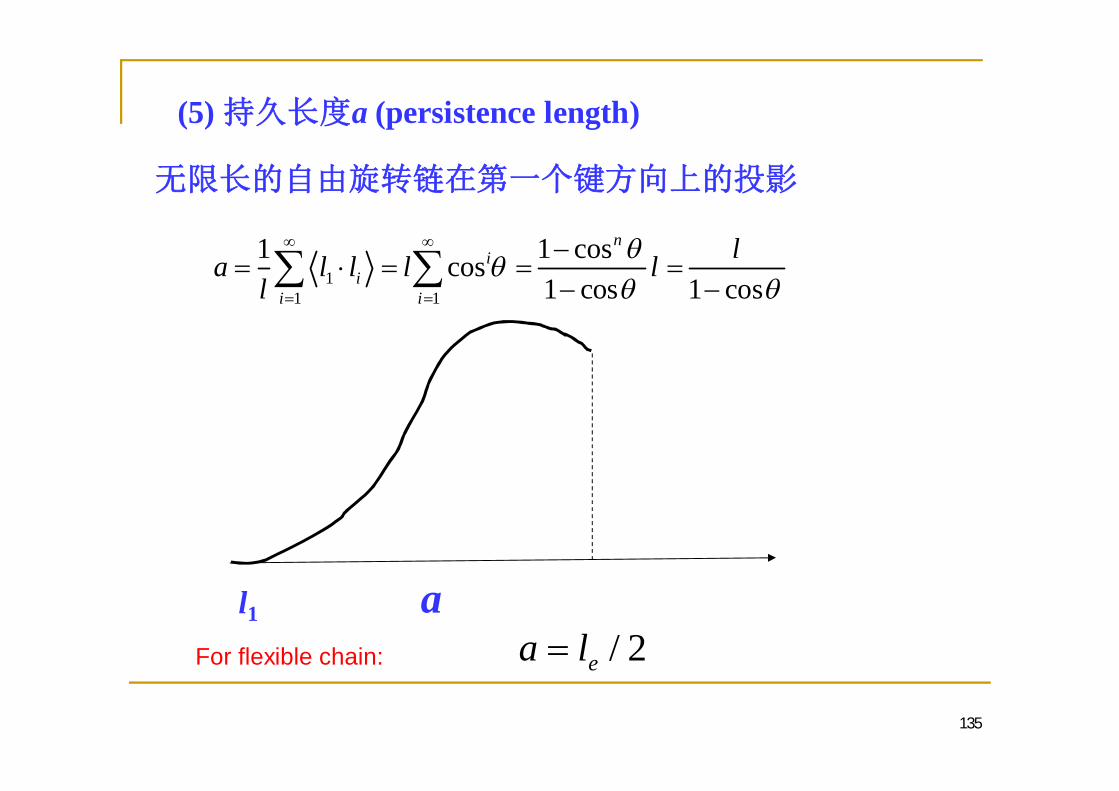
(5) a (persistence length)
11 1
1 1 coscos1 cos 1 cos
ni
ii i
la l l l ll
l1 a
135
/ 2ea lFor flexible chain:
2.2.4.2
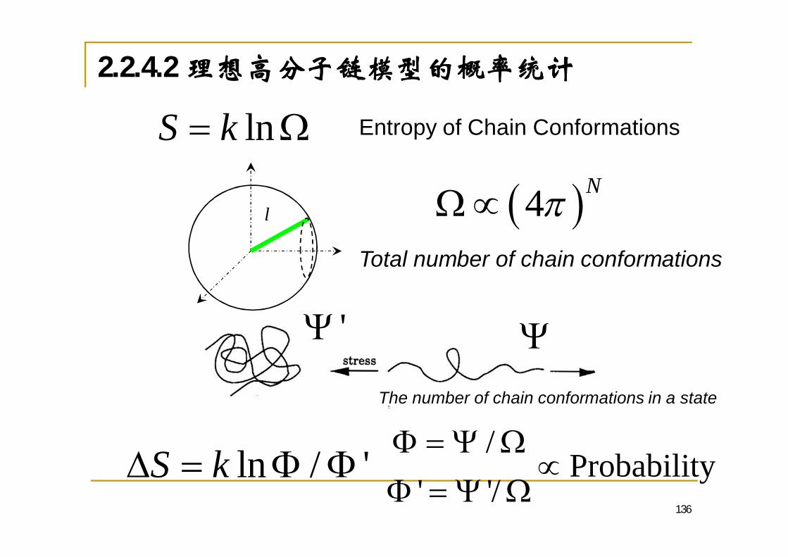
136
lnS k
4 N
ln / 'S k /Probability
' '/
Total number of chain conformations
Entropy of Chain Conformations
l
'
The number of chain conformations in a state

h (h)
h1, (h1)
…
h2, (h2) h3, (h3)
142
=

138
2 2
2 2gg
h h h dh
R R h dh
138ln / 'S k R R
h
h'
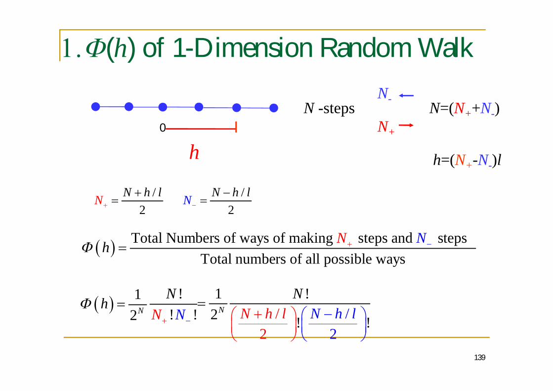
(h) of 1-Dimension Random Walk
139
0
h
N -stepsN-
N+
h=(N+-N-)l
N=(N++N-)
/2
N lN h /2
N lN h
Total Numbers of ways of making steps and stepsTotal numbers of all possible ways
h N N
12Nh
!! !N
N N /2
/2
1 !2 ! !
N N h l N h lN
140
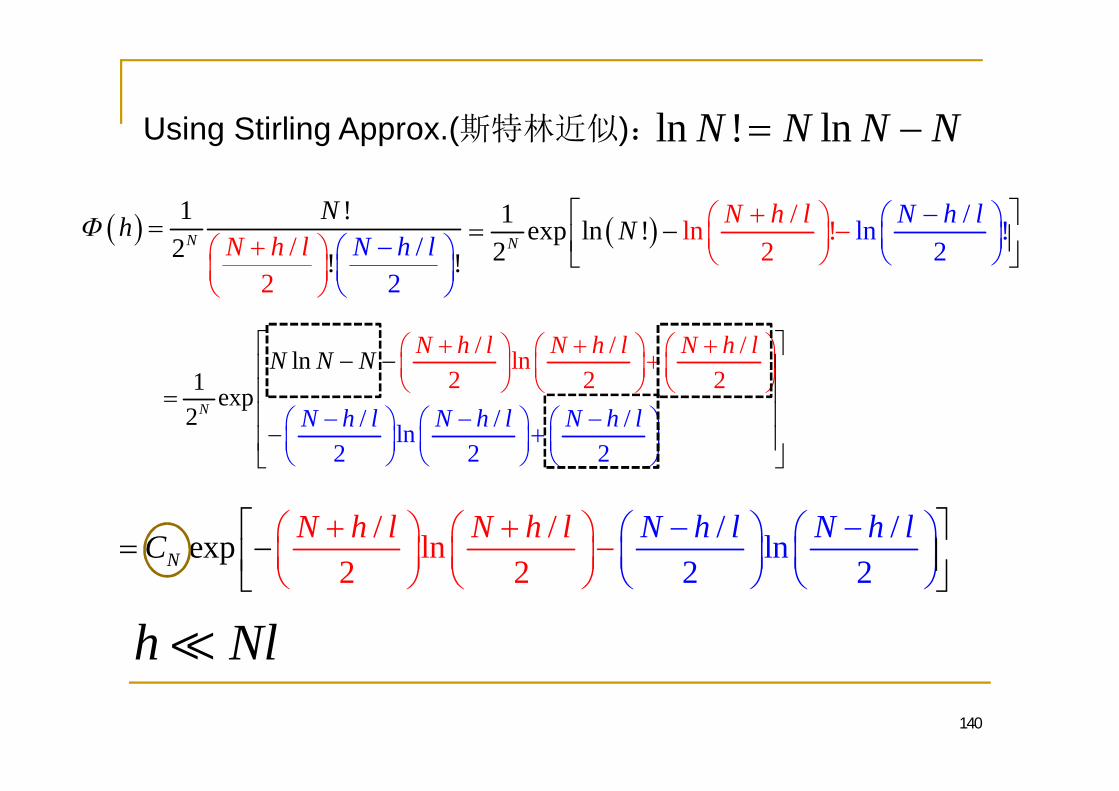
Using Stirling Approx.( ) ln ! lnN N N N
1 !2 !
2/ /!
2
N N h N h lh
lN 1 exp ln ! /ln /ln!
2!
22NN hN hl N l
/ / /ln
/ / /ln
2
ln1 e
2x
22
2p
2
2
N
N h l N h
N h l N h
l NN N
l N h l
N h l
/ /ln2
ex / /ln2
p22N
N h l N h lN hC l N h l
h Nl

141
2
2"exp2N
hh CNl
1 / 1 /l 1 / 1 /ln2
x n2 22
e pNh Nl h NlN Nh Nl h NlNC N
h Nl
21ln 12
y y y O
/y h Nl 1 11 ln'ex 12 2
p2
ln2N
N y N yy NNC y
1h dh
1/2 2
2 2
1 exp2 2
hhNl Nl
Normalization
Gaussian Distribution
1 ln 12
1 l'exp ln2
n 12N
N y y y yNC NN
22 112
11p2 2
x2
"eNN y y y N y yC y 2"exp
2NNC y
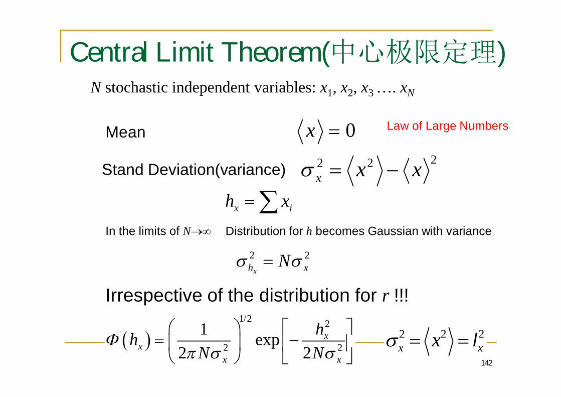
Central Limit Theorem( )
142
N stochastic independent variables: x1, x2, x3 …. xN
Mean
Stand Deviation(variance)
0x22 2
x x x
In the limits of N
x ih xDistribution for h becomes Gaussian with variance
2 2xh xN
Irrespective of the distribution for r !!!1/2 2
2 21 exp
2 2x
xx x
hhN N
2 2 2x xx l
Law of Large Numbers
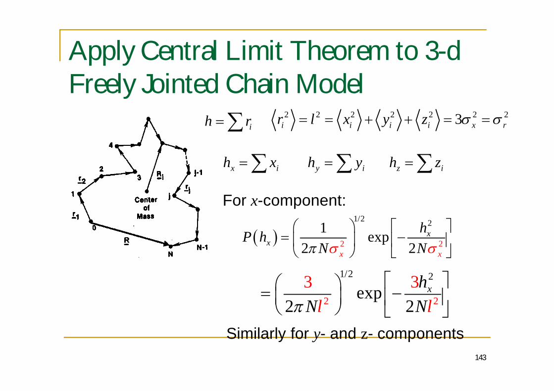
Apply Central Limit Theorem to 3-dFreely Jointed Chain Model
143
2 2 2 2 2 2 23i i i i x rr l x y z
x ih x
ih r
y ih y z ih z
For x-component:1/2
2
2
2
1 exp2 2
x
xx
x
hP hN N
Similarly for y- and z- components
1
2
2
2
/2
exp32 2
3 xhN Nl l

Overall Distribution for h
144
, ,x y z x y zh P h h h P h P h P h
Generalized to d-dimension:
3 d???
1/2 2
2 2, ,
3 3exp2 2
x y zR h h h Nl NR
l
3
2 2
/2 23 3exp2 2
hNl Nl
2 2 2 2x y zh h h h
145
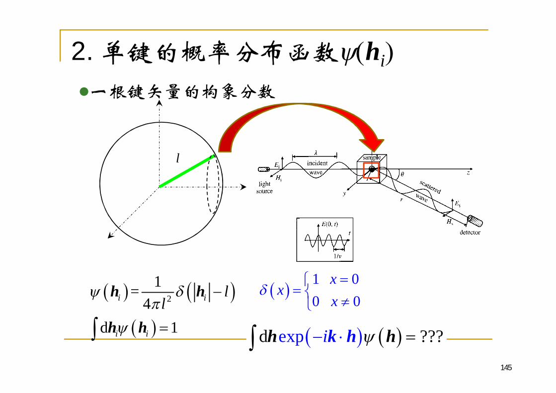
2. hi
l
2
1=4
d 1
i i
i i
ll
h h
h h
1 00 0
xx
x
ex ???pd ik hhh

&
146
d exp ih k h h
02 0 0
21 d d sin exp cod s4
ikh ll
hh h
22 0
1
0 1
1 d4
d d expx ih h l khhl
x
22 0
1 d2
1 ikh ikhe ei
h lkh
h hl
22 0
1 d 2 i2
s n kh hh h ll kh
22
1 2 sin2
l kll kl
sin klkl -30 -20 -10 0 10 20 30
-0.4
-0.2
0.0
0.2
0.4
0.6
0.8
1.0
sin(
kl)/k
l
kl
2
1=4
ll
h h
d exp ih k h h
= cos + ( )
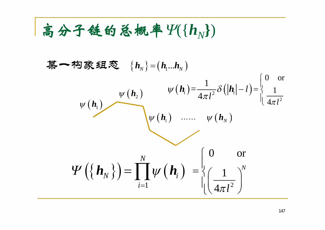
({hN})
147
1...N Nh h h
1
N
N ii
h h
1h2h
ih Nh……
2
0 or
14
N
l
21=
4i i ll
h h2
0 or1
4 l

=h (h, N)
148
:1
N
ii
h h
h, (h, N)
1 00 0
xx
x 31 d
2ie k xk=
1
N
ii
h h, Nh d . . . dd ih

Fourier
x
sin(
x) FT
f(x)
x
FT
iFT
iFT
f(x)=cos(ax)
F= ( )d if x F e x
149
F( )=f(x)=1
31 d
2ix e k xk
1 d2
iF f x xe x2
a aF
a

h (h, N)
150
31
1 21 d expd d ... d,
2
N
iN iiN ik kh h h hh hh
3 1 1
1 d e d ... p(2
d x )N i
Ni
iie ik h h k hh hk
31 d p
2 d ex
Nie ik h h hk k h
sind exp
kli
klh k h h
2
1=4i i l
lh h
1
N
N iih h
31 sind
2,
Ni kle
kN
lk hkh

h (h, N)
151
31 sind
2,
Ni kle
kN
lk hkh
2 2 2 2sin 1 exp6 6
NNkl k l Nk lkl
2
1/2 2
exp
exp4
ax bx dx
ba a
=1
2 d exp 6
, ,
=1
26
exp3
2
, ,
=3
2 exp3
2
12 d exp 6 x y zd dk dk dkk
, ,x y zdk
h
h
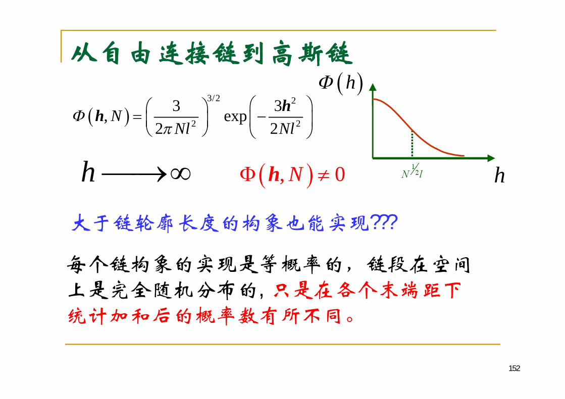
152
h , 0Nh
,
3/2 2
2 2
3 3, exp2 2
NNl Nl
hh
???
(h, N)
= ,
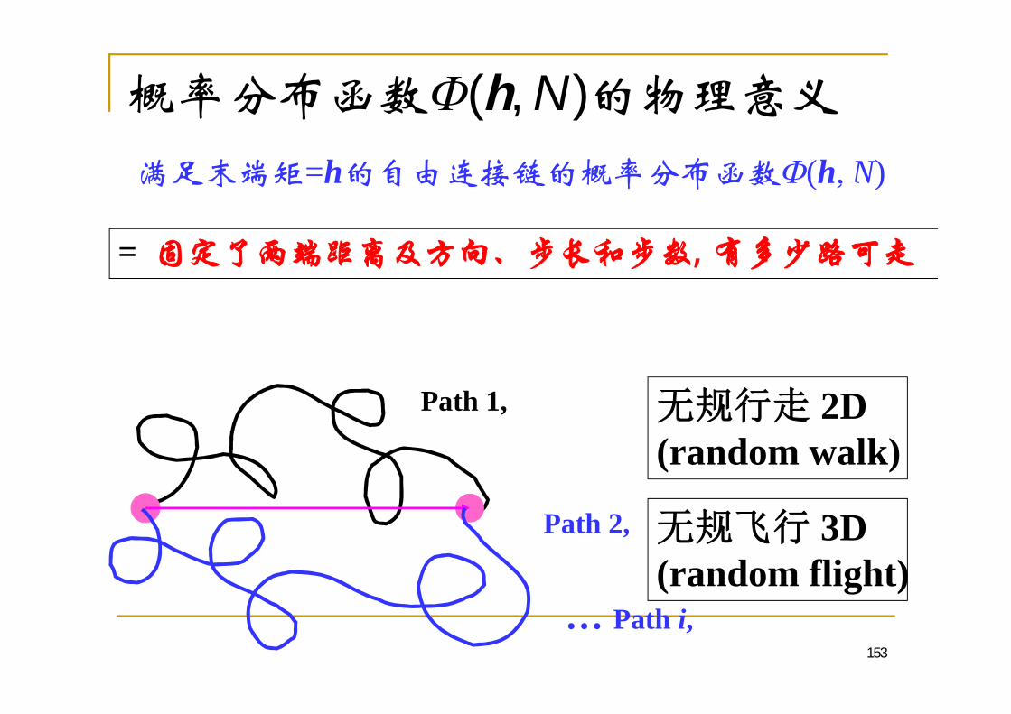
=h (h, N)
Path 1,
Path 2,
… Path i,
2D(random walk)
153
3D(random flight)

W(h, N)
RR’
W(h, N)
h
22
22/3
2 423exp
23, h
Nlh
NlNhW(R, N)
154
h
h

(h, N)
3/2 1/222
2 20
3 3 2 2exp 4 d2 2 3
h Nh h lNl N
hl
h
W(h, N)
h
,0
W h Nh
h*=(2N/3)1/2 l
155
2 210
2 1 !!d
2ax m
m m
me x x
a a
10
!dp axp
px e xa
< > < > /
3/ 2 22
2 20
2 2 23 3exp 4 d2 2
h h hNl N
h h Nll
>
< >=< > / ? ? ?

Applications of Gaussian Chain Model: Stretching of an Ideal Chain
156
3/22
2 2
3 3, exp2 2
g g
gg g
NN l N l
hh3/2
2
2 2
3 3, , exp2 2g g g g
g g
N N N NN l N l
hh h
2
2 2
3 3 3( , ) ln( ) ln2 2 2g B B B g
g g
S N k k k NN l N lhh
23( , ) Bg
g
G Nh
k TN l
hf h
2
2
3( , ) ( )2g B g
g
G N U TS k T G NN lhh
, , /g g gN N Nh h
lnS k h
=???
kf x
ln / 'S k
/' '/

157
ri-1ri
hi
hi
ri-1
ri+1
ri hi+1
3/ 2 2
2 2
33, exp2 2
ii l l
hh
3/2 2
2 21
3 3exp2 2
gNi
iil l
hh
3/22
2 2
3 3, exp2 2
g g
gg g
NN l N l
hh
2 2 2 2 2
0i gh h l b l
2 2 2 2g g g g
h Nl N l N h
g
NN
31
1 21 d expd d ... d,
2
N
iN iiN ik kh h h hh hh

Two Definitions of Segment
(1) Kuhn Segment (Kuhn )le
lg le158
2maxeh l L
(2) Effective Gaussian Segment ( )lg
,
lg le
159
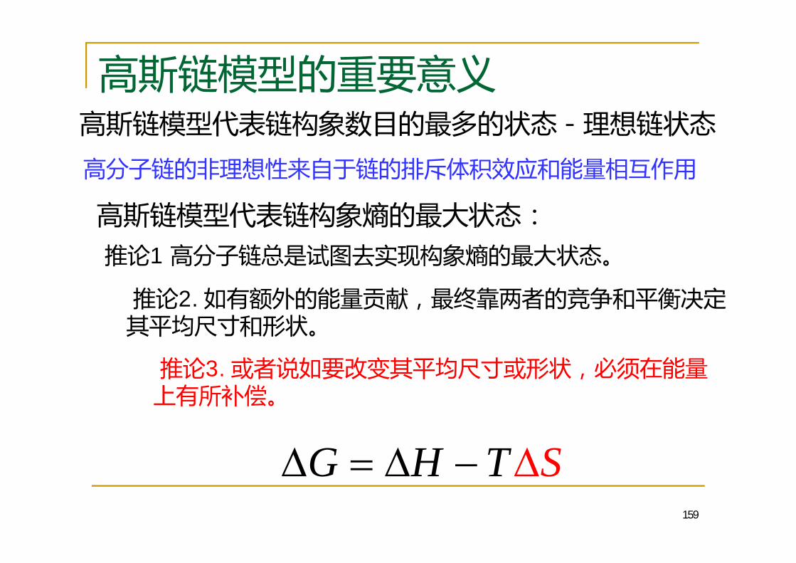
G H ST
1
3.
2.

I
160
2 1RW ~R N
3/2 2
2 21
33 exp2 2
gNi
ii l l
hh
23 /21
2 21
33 exp2 2
g gN Ni i
nb bR R
2
2 0
3exp2
gN nconst dnb n
R
2 2l b
Path Integral( )Edward’s Minimum Model
interaction energyih H Mean-field Free Energy
,=
6,, =
32
exp3
2

Appendix. Diffusion Equation
161
1Nh
h
has a probability of 1/zof occurring
, =1
, 1
=
, 1 = ,, ,
+12
,
1= 0
1=
13
2 ,= 6
,
, =3
2 exp3
2
Diffusion Equation
Each l has a directions of zl
h>>l, N>>1

II: blob
162162 162
2 2 6/5SAW ~ ~R N N
3/2 2
2 2
3 3, exp2 2
NNl Nl
hh2 1RW ~R N
???

(Blob)
163
blob
Blob
blob
~ BNG k Tg
2 1RW ~R N 2 2
SAW ~R N

2.2.5 -2.2.5.1
164
1 1
sin1 N Ni j
i j i j
gN
k r rk
k r r
2 2
1 1
1 16
N N
i ji jN
k r r
2
1 1
21 26
N N
i ji j i
N NN
k r r2 2 2
1 1
N N
i j gi j i
N Rr r
22 221
3 gN RNN
k
2 2sin 16
kl k lkl
l12
sing klkkl
22
13 gN Rk
sin j iij
j i
gk r r
kk r r
1/k r

2.2.6.2
165
2 2gi j i j lr r
i j|i-j|
2 2
0 0
1 d d 16
N N
i jg i jN
kk r r
0
2g
2
0
1 d d 16
N Ni j li j
Nk
2 2g
0 0
1 d d exp6
N N li i jj
Nk
2 2
00 0
1 d d expN N
gi j RN
i jk
g
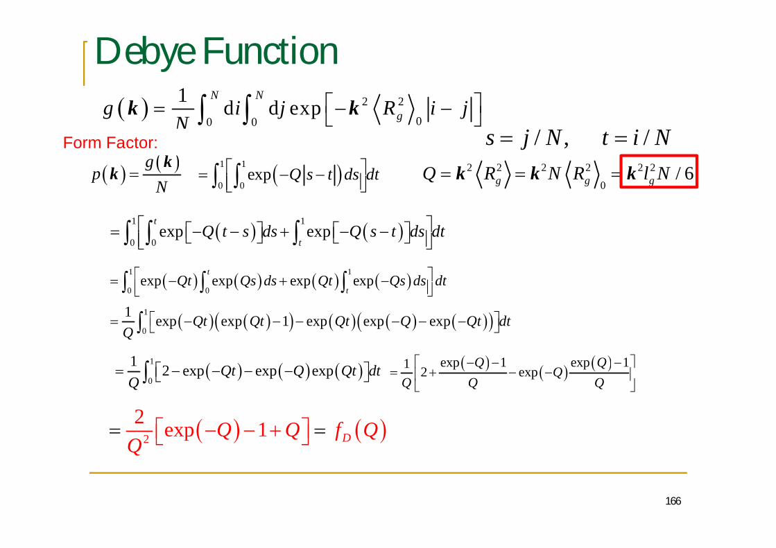
Debye Function
166
gp
Nk
k
/ , /s j N t i N
2 2
00 0
1 d d expN N
gg i j R i jN
k k
2 2 2 2 2 2
0/ 6g g gQ R N R l Nk k k
1 1
0 0exp exp
t
tQ t s ds Q s t ds dt
1 1
0 0exp exp exp exp
t
tQt Qs ds Qt Qs ds dt
1
0
1 exp exp 1 exp exp expQt Qt Qt Q Qt dtQ
1
0
1 2 exp exp expQt Q Qt dtQ
exp 1 exp 11 2 expQ Q
QQ Q Q
22 exp 1 DQ Q f Q
Q
Form Factor:1 1
0 0exp Q s t ds dt

Debye
167
2 2D D gg Nf Q Nf Rk k
22 1Q
Df Q e QQ
2 2(1) 1gRk2 3
2
2 1 / 2! / 3! 1 1 / 3Df Q Q Q Q Q QQ
221
3D gg Nf Q N Rkk
22 2 2/ 1
3D g gp g N f R Rkk k kForm Factor:
2 2gQ Rk

168
2 2(2) 1gRk
2
2 21QDf Q e Q
Q Q
22 2 2
22 2 2 2
1 / 3 1
2 / 1
g g
D
g g
N R Rg Nf Q
N R R
k kk
k k k
Ornstein-Zernike
2 21 / 2g
NgR
kk
2 2 2 2 / 6g gQ R l Nk k
2 2
11 / 2g
pR
kkor
Structure Factor Form Factor
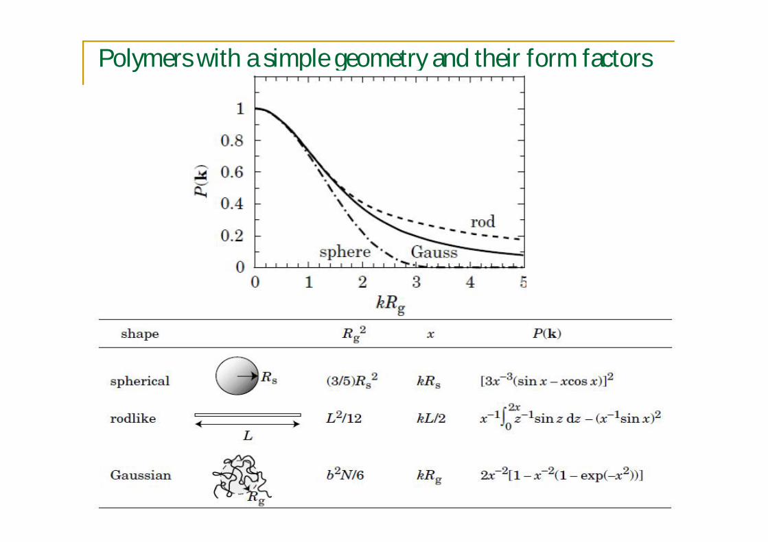
Polymers with a simple geometry and their form factors
169

170
Sphere
Rod

Form Factor ( )of a Real Chain
171
2 2
11 / 2g
pR
kk
???
2p kk1gkR
172
1/1
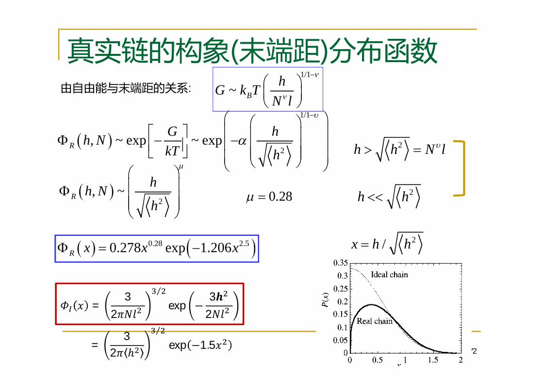
~ BhG k T
N l1/1
2, ~ exp ~ expR
G hh NkT h
2h h N l
2, ~R
hh Nh
2h h0.28
0.28 2.50.278 exp 1.206R x x x2/x h h
:
=3
2exp
32
=3
2 exp 1.5
173
1.
2.
(1)
(2)
(3)
(5)
(4)

-
174174
Gaussian Chain Model
Entropy of Chain Conformations
Mechanic Properties
Scattering Theory (R> /20)
h, (h, N)
h
h
2
2
3( , )2conf g B
g
S N k CN lhh
20 eR l L
2 2 2~R N l
Scaling Concept & Blob Model
2 20
R NlIn solution:
2 2
11 / 2g
pR
kk
23 Bk TNlhf
~ BNG k Tg
, =3
2exp
32


![montary policy-group5 [兼容模式] - Fudan Universityjpkc.fudan.edu.cn/picture/article/237/1a/60/b6e9c3d24cc68d90191773... · MONETARY POLICY: THEORY, APPLICATION During Financial](https://static.documents.pub/doc/80x56/5b062b627f8b9a56408b4c5c/montary-policy-group5-fudan-policy-theory-application-during.jpg)


