52
Reservoirology & Graphs rev 2 Riccardo Rigon R., Marialaura Bancheri, Francesco Serafin From August 2016 Sara di Nambrone, 1 Agosto 2016
| Date post: | 16-Apr-2017 |
| Category: |
Education |
| Upload: | riccardo-rigon |
| View: | 205 times |
| Download: | 1 times |

Reservoirology & Graphs rev 2
Riccardo Rigon R., Marialaura Bancheri, Francesco Serafin
From August 2016
Sara
di
Nam
bro
ne,
1
Agost
o 2
01
6

!2
Rational
In literature we found several representations of the water budget as reservoirs.
However these representations usually are not very explicative.
hillslope to the dynamic saturation area in the riparian zoneand underlying groundwater. The approach connects the twoupper storage units which conceptualize storage in theriparian peat soils (Ssat) and the freely draining podzols on thehillslopes (Sup). Direct mapping of the spatial extent ofsaturated soils in the valley bottom – that were hydrologicallyconnected to the stream network during different wetnessconditions (see Ali et al., 2014) – allowed us to develop andfit a simple antecedent precipitation index-type algorithmwhich could explain around >90% of the variability (Birkelet al., 2010). This algorithm was applied to create acontinuous time series of the expanding and contractingdaily saturation area extent (dSAT) (Figure 4). This dSATtime series was used as model input to dynamically distributedaily precipitation inputs between the storage volumes in thelandscape-based (hillslope (Sup) and saturation area (Ssat))model structure (Soulsby et al., 2015).Like Birkel et al. (2015), we used reservoirs that could
become unsaturated allowing storage deficits to occur. Theriparian area is normally saturated (i.e. with positive storage),but can have small deficits following prolonged dry periodsin summer. In the upper stores, water levels below a certainthreshold can only be further depleted by transpiration and nolateral flow to the riparian area will be generated. Incomingprecipitation fluxes arefirst intercepted and reduced by PET –if available. The remaining effective precipitation fills the
uppermost storages and captures soil moisture-relatedthreshold processes of runoff generation (Tetzlaff et al.,2014). Consequently, Sup was often in deficit, but in wetterperiods would fill and spill into Ssat, which usually has low orno deficit generating stream flow.The storages S are state variables in the model, and we
describe the following fluxes and calibrated parametersshown in Figure 4. The unsaturated hillslope reservoir Sup isdrained (fluxQ1 inmmd!1) by a linear rate parameter a (d!1)and directly contributes to the saturation area store Ssat. Therecharge rate R (mm d!1) to groundwater storage Slow islinearly calculated using the parameter r (d!1). The Slow storegenerates runoff Qlow (mm d!1) contributing to totalstreamflow Q (mm d!1) using the linear rate parameter b(d!1). The runoff component Qsat (in mm d!1), which isgenerated nonlinearly from Ssat, conceptualizes saturationoverland flow using the rate parameter k (d!1) and thenonlinearity parameter α (—) in a power function-typeequation (Figure 2).Q is simply the sumofQsat andQlow. Theuse of linear or non-linear parameters was based on priorsystematic tracer-aided multi-model testing for similarcatchments in the Scottish Highlands (Birkel et al., 2010;Capell et al., 2012). In particular, the non-linear conceptu-alization of Qsat has a physical basis in the dynamicexpansion of the saturation area and fluxes that generatestorm runoff. Likewise, the linear nature of Q1 and R reflect
Figure 4. Conceptual diagram of the model with equations and calibrated parameters (in blue)
2487CONNECTIVITY BETWEEN LANDSCAPES AND RIVERSCAPES
Copyright © 2016 The Authors Hydrological Processes Published by John Wiley & Sons Ltd. Hydrol. Process. 30, 2482–2497 (2016)
Take an example of the figure above from Birkel et al. 2011. It pretends to
be explicative and from it we should be able to derive easily the set of mass
conservation that rule the system. However, this action requires a little of
analysis. A more complicate set of reservoirs is shown in the next slide.
Rigon et al.
Introduction

!3
1 Figure 1. Flow diagram for Prediction in Ungauged Basins 2
3
4 Figure 2. Model structure derived from DEM, showing three landscape classes and the 5 groundwater system connecting them. 6
7
β
D
Ks
Kf
Si
Su,max
X
22
Hydrol. Earth Syst. Sci. Discuss., doi:10.5194/hess-2016-433, 2016Manuscript under review for journal Hydrol. Earth Syst. Sci.Published: 29 August 2016c� Author(s) 2016. CC-BY 3.0 License.
Savenije, H. H. G., & Hrachowitz, M. (2016). Opinion paper: How to make our models more physically-based. Hydrology and Earth System Sciences Discussions, 1–23. http://doi.org/10.5194/hess-2016-433
Rigon et al.
Introduction

!4
The idea is to build an algebra of objects to represent (water) budgets
giving a clear idea of the type of interactions that the budget is subject
to.
Any symbol should correspond to a mathematical term or a group of
mathematical terms. The number and the collocation of parameters of
the models should be clear.
There is a better way to represent reservoir interactions ?
Rigon et al.
Introduction

!5
Introduction
Rigon et al.
At the beginning, I was trying to develop my own algebra
However I realised soon that Petri Nets cover the same area. I
had to adjust somewhat my perception because in Petri Nets,
storages (called places) are represented as circles, and fluxes
(called transitions) are represented as small rectangle. I
made, in our case, the rectangles small square. But the
concept and the rules remains the same. All of it resulted in a
graphical algebra a little more verbose than my original one,
but, at the end, more explicative.

!6
The other relevant difference
Introduction
Rigon et al.
The normal Petri Nets, are discrete Petri net, and do not have
time. Instead, we are dealing with dynamical systems and, having
time inside, is a necessity for us. So, our, are time continuous
Petri nets (TCPN).
Blätke, M. A., Heiner, M., & Marwan, W. (2011). Petri Nets in System Biology (pp. 1–108). Msgdeburg Universität.
2.2. Standard Petri Net 5
the integration of qualitative, continuous and stochastic information. This allows the representationof di↵erent kinetic processes and di↵erent data types. Petri nets link structural and dynamic analysistechniques to investigate and validate a model such as graph theory, application of linear algebra tocheck a model and simulation methods. This facilitates the performance of simulation studies to explorethe time-dependent dynamic behaviour, the in-depth analysis of structural criteria and the state spaceof a model.
2.2 Standard Petri Net
A Petri net is represented by a directed, finite, bipartite graph, typically without isolated nodes. Thefour main components of a general Petri net are: places, transitions, arcs and tokens; see Figure 2.3,A.
Figure 2.3: Petri Net Formalism. Petri nets consist of places, transitions, arcs and tokens (A). Justplaces are allowed to carry tokens (B). Two nodes of the same type can not be connected with each other(C). The Petri net represents the chemical reaction of the water formation (D). A transition is enabled andmay fire if its pre-places are su�ciently marked by tokens.
Places are passive nodes. They are indicated by circles and refer to conditions or states. In abiological context, places may represent: populations, species, organisms, multicellular complexes,single cells, proteins (enzymes, receptors, transporters, etc.), molecules or ions. But places could alsoembody temperature, pH-value or membrane potential; see also Section 3.3.1. Only places are allowedto carry tokens; see Figure 2.3, B.
Tokens are variable elements of a Petri net. They are indicated as dots or numbers within a placeand represent the discrete value of a condition. Tokens are consumed and produced by transitions; seeFigure 2.3, D. In biological systems tokens refer to a concentration level or a discrete number of aspecies, e.g., proteins, ions, organic and inorganic molecules. Tokens might also represent the value ofphysical quantities like temperature, pH value or membrane voltage that e↵ect biological systems. APetri net without any tokens is called “empty”. The initial marking a↵ects many properties of a Petrinet, which are considered in Chapter 2.
Transitions are active nodes and are depicted by squares. They describe state shifts, system eventsand activities in a network. In a biological context, transitions refer to (bio-)chemical reactions,molecular interactions or intramolecular changes; see also Section 3.3.1. If a place is connected byan arc with a transition, the place (transition) is called pre-place (post-transition). If a transitionis connected by an arc with a place, the transition (place) is called pre-transition (post-place); seeFigure 2.4. Transitions consume tokens from its pre-places and produce tokens within its post-placesaccording to the arc weights; see Figure 2.3, D.

!7
For information about
normal Petri Nets, a good reference is
Murata, T. (1989). Petri Nets: Properties, Analysis and Applications. Proceedings of the IEEE, 77(4), 1–40.
Petri Nets
Rigon et al.

!8
So …. our graphical language
Places correspond to storages, for instance the volume of
water in groundwater, or the energy content of the same
groundwater, or its momentum content. To distinguish the
various “storages” the circle has a variable specification. It
is intended that a graph is composed of places that
contains the same type of quantities, mass, momentum or
energy. Places can be coloured, and the same color used to
represent the same physical place but in different types of
budgets.
Places
Rigon et al.

!9
So …. our graphical language
Each one of the places depicted represents the time
variation of the named quantity. For instance the place at
the center represents
Places
Rigon et al.

!10
Symbols for reservoirs systems
an arc (positive in the direction of the arrow) connect a place with a transition and viceversa. In our case a transition is a flux. By convention, the arc is of the same color of the place from where it exits.
Rigon et al.
Transitions or Fluxes
A flux (transition) is represented by a square the symbols inside represents the type of flux

!11
So, a linear reservoir
is represented as follows:
Rigon et al.
A simple example to begin with
with a one-to one correspondence with the equation below:

!12
or, BTW
Rigon et al.
A simple example to begin with
if we want to use colors

!13
Symbols
a linear flux (positive in the direction of the arrow).
an external forcing, for instance precipitation but can be evapotranspiration, if this is measured is represented by a
It is a term of the r.h.s of the budget equation
a non linear flux (positive in the direction of the arrow).
The symbol indicating non-linearity alone
Rigon et al.
Arcs

!14
so, the previous linear budget could be
Rigon et al.
A simple example to begin with
when rainfall is an assigned time series, i.e. a flux boundary condition

!15
Who is connected with whom ?
Rigon et al.
Allowed connections (with colors)
So we can have
but not other type of connections
transition —> place
place —> transition
place —> transition —> place
transition —> place —> transitions

!16
Who is connected with whom ?
Rigon et al.
One transition can be connected with more than one place, implying the existence of a partition coefficient
One place can have more that one transitions, also implying some partition coefficient

!17
One flux that interacts back:
simply means that
where B is some metastable place
Who is connected with whom ?
Rigon et al.

!18
Soulsby, C., Birkel, C., & Tetzlaff, D. (2016). Modelling storage-driven connectivity between landscapes and riverscapes: towards a simple framework for long-term ecohydrological assessment. Hydrological Processes, 30(14), 2482–2497. http://doi.org/10.1002/hyp.10862
hillslope to the dynamic saturation area in the riparian zoneand underlying groundwater. The approach connects the twoupper storage units which conceptualize storage in theriparian peat soils (Ssat) and the freely draining podzols on thehillslopes (Sup). Direct mapping of the spatial extent ofsaturated soils in the valley bottom – that were hydrologicallyconnected to the stream network during different wetnessconditions (see Ali et al., 2014) – allowed us to develop andfit a simple antecedent precipitation index-type algorithmwhich could explain around >90% of the variability (Birkelet al., 2010). This algorithm was applied to create acontinuous time series of the expanding and contractingdaily saturation area extent (dSAT) (Figure 4). This dSATtime series was used as model input to dynamically distributedaily precipitation inputs between the storage volumes in thelandscape-based (hillslope (Sup) and saturation area (Ssat))model structure (Soulsby et al., 2015).Like Birkel et al. (2015), we used reservoirs that could
become unsaturated allowing storage deficits to occur. Theriparian area is normally saturated (i.e. with positive storage),but can have small deficits following prolonged dry periodsin summer. In the upper stores, water levels below a certainthreshold can only be further depleted by transpiration and nolateral flow to the riparian area will be generated. Incomingprecipitation fluxes arefirst intercepted and reduced by PET –if available. The remaining effective precipitation fills the
uppermost storages and captures soil moisture-relatedthreshold processes of runoff generation (Tetzlaff et al.,2014). Consequently, Sup was often in deficit, but in wetterperiods would fill and spill into Ssat, which usually has low orno deficit generating stream flow.The storages S are state variables in the model, and we
describe the following fluxes and calibrated parametersshown in Figure 4. The unsaturated hillslope reservoir Sup isdrained (fluxQ1 inmmd!1) by a linear rate parameter a (d!1)and directly contributes to the saturation area store Ssat. Therecharge rate R (mm d!1) to groundwater storage Slow islinearly calculated using the parameter r (d!1). The Slow storegenerates runoff Qlow (mm d!1) contributing to totalstreamflow Q (mm d!1) using the linear rate parameter b(d!1). The runoff component Qsat (in mm d!1), which isgenerated nonlinearly from Ssat, conceptualizes saturationoverland flow using the rate parameter k (d!1) and thenonlinearity parameter α (—) in a power function-typeequation (Figure 2).Q is simply the sumofQsat andQlow. Theuse of linear or non-linear parameters was based on priorsystematic tracer-aided multi-model testing for similarcatchments in the Scottish Highlands (Birkel et al., 2010;Capell et al., 2012). In particular, the non-linear conceptu-alization of Qsat has a physical basis in the dynamicexpansion of the saturation area and fluxes that generatestorm runoff. Likewise, the linear nature of Q1 and R reflect
Figure 4. Conceptual diagram of the model with equations and calibrated parameters (in blue)
2487CONNECTIVITY BETWEEN LANDSCAPES AND RIVERSCAPES
Copyright © 2016 The Authors Hydrological Processes Published by John Wiley & Sons Ltd. Hydrol. Process. 30, 2482–2497 (2016)
Birkel, C., Soulsby, C., & Tetzlaff, D. (2011). Modelling catchment-scale water storage dynamics: reconciling dynamic storage with tracer-inferred passive storage. Hydrological Processes, 25(25), 3924–3936. http://doi.org/10.1002/hyp.8201
Rigon et al.
A more complicate example
We can represent the initial system as follows:

!19
Now, start to read it. There are three ordinary differential equations (ODEs), represented by the three places, and here also colored in different ways. Moreover, there is a given input (J). One of the equations, contains a non linear term. The others are linear. Because J is split into two directions, a partition coefficient is necessary.
Rigon et al.
One circle is one ODE

!20
The equations, in one-to-one correspondence to the net are:
Where the fluxes form is note yet specified.
Rigon et al.
One circle is one ODE

!21
The missing knowledge can be given by a table of this type:
where 7 parameters are given, and the type on non linearity present in equation (2) is specified. J(t) is given. If also ET is measured (as actually happened in the original paper, parameters reduce to 5).
Rigon et al.
Topology must be completed
!22
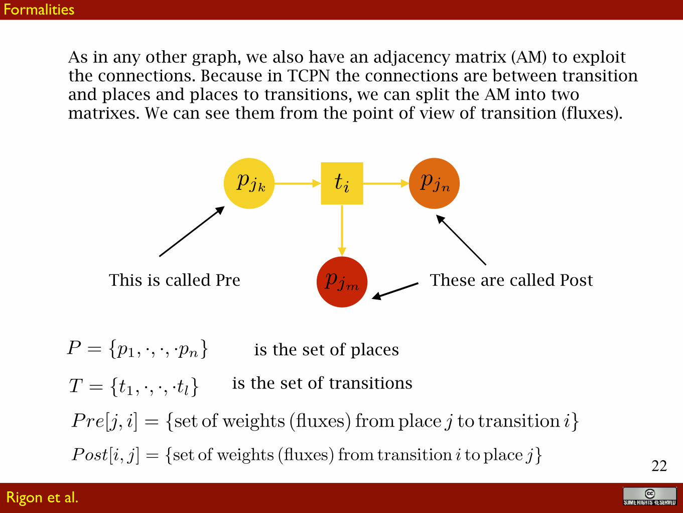
As in any other graph, we also have an adjacency matrix (AM) to exploit the connections. Because in TCPN the connections are between transition and places and places to transitions, we can split the AM into two matrixes. We can see them from the point of view of transition (fluxes).
This is called Pre These are called Post
is the set of places
is the set of transitions
Formalities
Rigon et al.

!23
is the set of places
is the set of transitions
Pre is a matrix n x l (rows are for the places, column are for the
transitions), and to each couple is associated a flux, or, in a more abstract
way to say it, it is:
Where represents a space of allowed fluxes expressions
Post is a matrix l x n
Both Pre and Post are adjacency matrixes with weighted entries
Rigon et al.
Formalities
If

!24
So, we can try a first definition by saying that a TCPN is a 5-tuple:
where S is the set of tokens present in places (at any specific time, including the initial one).
The set
is said the preset of . The set:
the postset of
Navarro-Gutierrez, M., Ramirez-Trevino, A., & Gomez-Gutierrez, D. (2016). Modelling the behaviour of a class of dynamical systems with Continuous Petri Nets (pp. 1–6). Presented at the 2013 IEEE 18th Conference on Emerging Technologies & Factory Automation (ETFA), IEEE. http://doi.org/10.1109/ETFA.2013.6647992
Rigon et al.
Formalities

!25
Actually, we introduced a few new elements here (besides places, transitions, arcs, tokens):
a Table of association between fluxes and their expression:
Expressions or, possible algebraic form of the fluxes
Rigon et al.
Table of association

!26
Rigon et al.
Table of association
So, we can say that, the full description of system is a 7-tuple:
where
is a vocabulary of fluxes and symbols, with their semantic
is the set of expressions where the symbols are combined to produce the fluxes form and, ultimately the fluxes values
To build the vocabulary, we used simple table, but a more rigorous approach could be envisioned by looking at the Basic Modelling Interface (BMI)

!27
Introducing some of the next networks we will also show explicitly what the previous sets and matrixes are.
A TCPN identifies a a coupled set of ordinary differential equations, in number equal to the rank of the places. They are:
Rigon et al.
Formalities
In practice, Post and Pre are sparse matrixes, and it could be convenient to store them in triplets
where expression, eventually are mapped to real values when expressions are evaluated.

!28
Every modelling solution is actually a compound. So the blue graph below on the right can be seen as a “coarse graining” of the one on the left.
To signify compounds the normal Petri net graphics use a sign, which we will use, instead to indicate sink/source effects.
Rigon et al.
Compounds

!29
thus, if the linear water budget below contains also a sink/source one
Rigon et al.
Sources/Sinks
it can be represented as follows:
!30
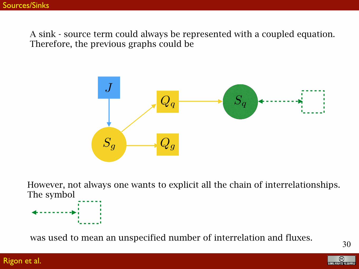
A sink - source term could always be represented with a coupled equation. Therefore, the previous graphs could be
However, not always one wants to explicit all the chain of interrelationships. The symbol
was used to mean an unspecified number of interrelation and fluxes.
Rigon et al.
Sources/Sinks

!31
We can have also systems of equations, formally of the same type, but parametrised by some variable, for instance, one case is that of the age-ranked water budget:
e.g. Rigon and Bancheri, 2016,
where the water volumes are separated according to water age
Rigon et al.
Parameterised equations

!32
In this case, instead of representing the equations with (unspecified) many graphs, we use only one, but with shadows or borders.
Rigon et al.
Parameterised equations

!33
When dealing with cases in which some physics-chemical reaction can be reverted, the case can be represented as a loop:
And simplified, as:
Rigon et al.
More complicate topologies

!34
Rigon et al.
Coupled equations: the single reservoir water budget
The single reservoir water budget has been a little complicated with respect to the simpler one in previous slides, to introduce evapotranspiration ad percolation loss. Both precipitation and percolation are assigned as flux boundary conditions.
!35
Rigon et al.
Coupled equations: the single reservoir energy budget
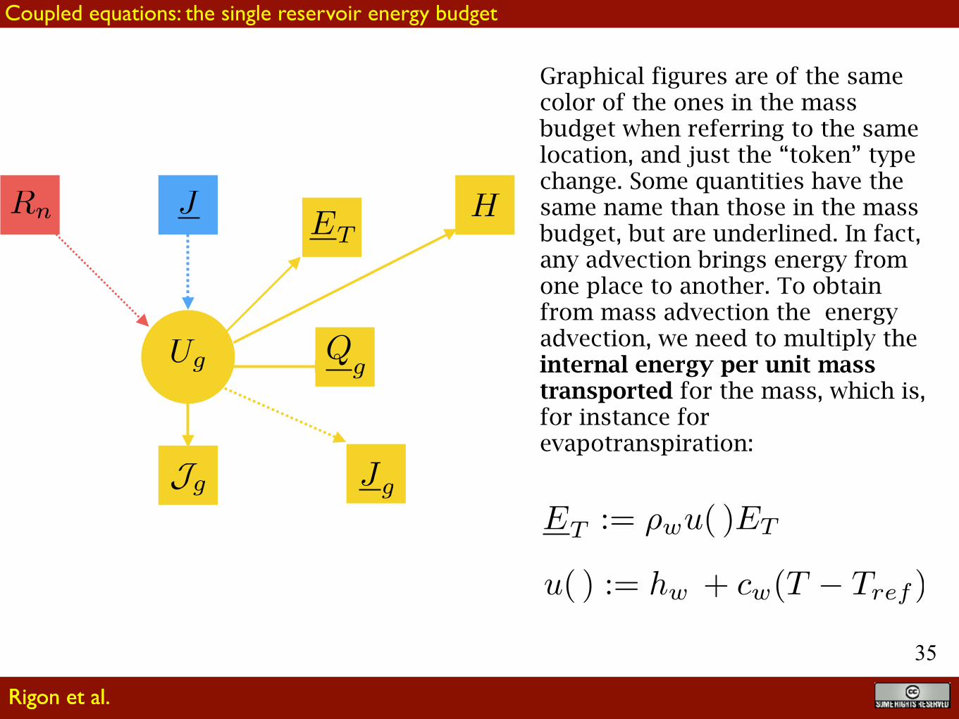
Graphical figures are of the same color of the ones in the mass budget when referring to the same location, and just the “token” type change. Some quantities have the same name than those in the mass budget, but are underlined. In fact, any advection brings energy from one place to another. To obtain from mass advection the energy advection, we need to multiply the internal energy per unit mass transported for the mass, which is, for instance for evapotranspiration:
Rigon et al.

!36
Rigon et al.
Coupled equations
The energy budget contains other terms, beyond the advective fluxes.
• Radiation, • thermal convective fluxes, • conduction
Radiation is given here as an external flux. This is not completely true, because it is actually a net budget which involve also the temperature of surfaces.
Rigon et al.

!37
Rigon et al.
Coupled equations
A single reservoir water budget with Evapotranspiration. Its equation is
As said, both J and Jg are assigned
Rigon et al.

!38
Rigon et al.
Coupled equations
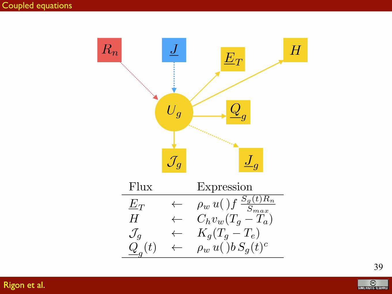
The fact that Evapotranspiration expression contains the net radiation, suggests that the budget can be modified as follows
where the symbol
tells that Rn does not enter in the budget but it is one of its parameters the dotted line means that it is an assigned boundary condition.
Rigon et al.
!39
Rigon et al.
Coupled equations
Rigon et al.

!40
Rigon et al.
Coupled equations
The two coupled budget can be represented as above. Arcs of the energy budget are weighted, in order to transform the quantity advected in energy. J in this case is not partitioned because the weight also implies it. The global graph look simpler than the single two.
Rigon et al.

!41
Rigon et al.
Coupled equations
Shadows in the water budget mean that the water budget is parametrised, and represents actually a group of equations.

!42
Now assume to have a river network
Consider the path starting in A1, for example. It can be decomposed into steps (states)
and we can write the water budget for each of them.
Rigon et al.
River Networks

!43
The Petri scheme can be
Rigon et al.
River Networks

!44
The full network interactions can be represented as follows
Rigon et al.
River Networks

!45
It can be simplified as shown above
Rigon et al.
Simplifications
!46
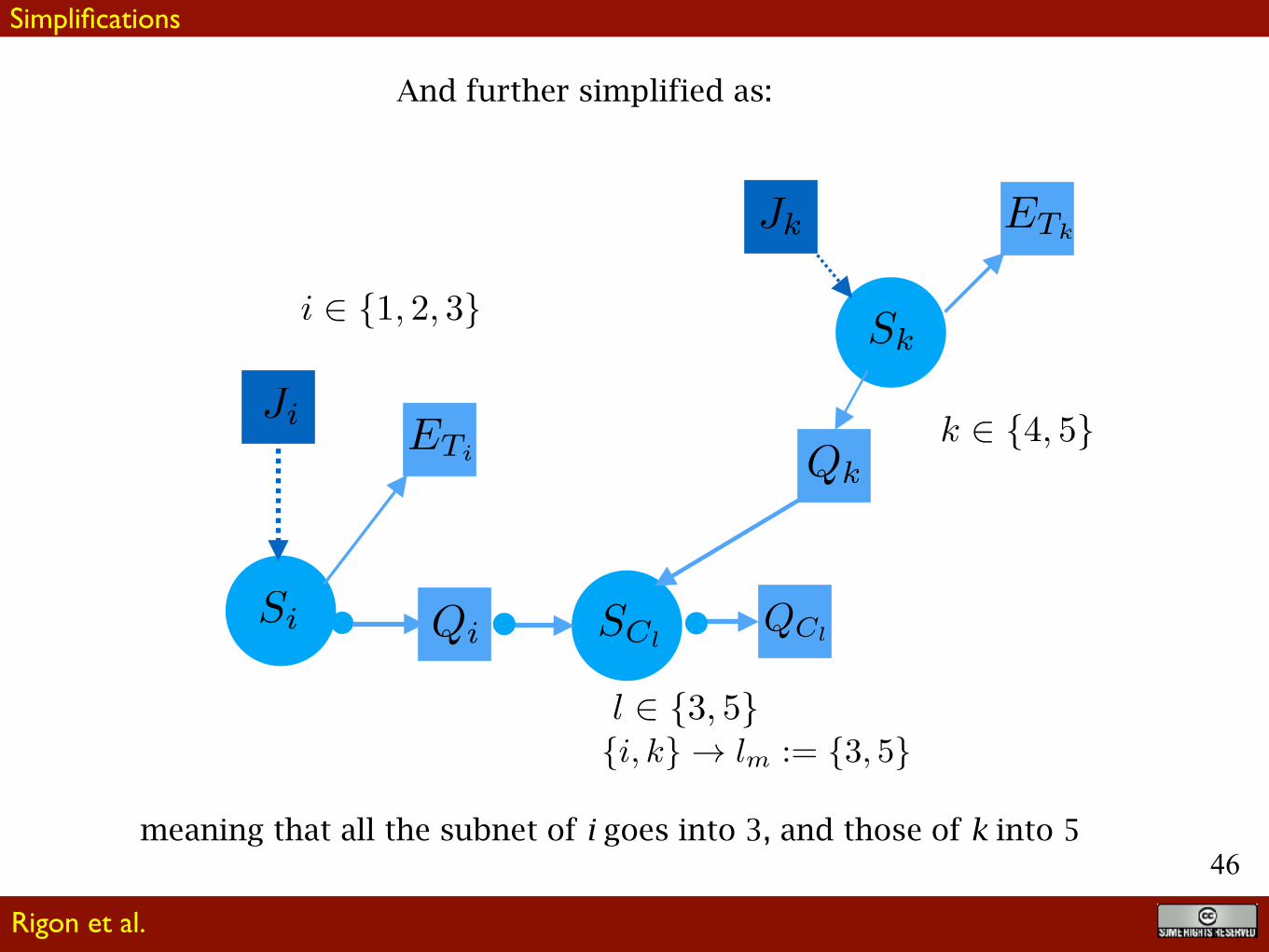
And further simplified as:
meaning that all the subnet of i goes into 3, and those of k into 5
Rigon et al.
Simplifications

!47
Here we introduce a space explicit place/
The difference is that the storage in channels has a spatial curvilinear coordinate. Tributary’s water enters the channel at some “x”, and exit at the last downstream x.
Rigon et al.
Space explicit places

!48
The full network interactions or as below.
A typical case is when channel is described by a width function, or when the dynamics of water is modeled by a 1d - de Saint-Venant equation.
Rigon et al.
Space explicit places

!49
The network above can be simplified as
where it is assumed that each i outflow has a coordinate x associated.
Rigon et al.
Space explicit places simplified

!50
The network with a space explicit channel is, at the end,
particularly simple. But it is easy to produce more complicate
configurations, especially if a single hydrologic response unit
(HRU) is subdivided in many interconnected reservoirs.
Rigon et al.
Comments

!51
Conclusion
We hope to have defined a group of signs able to simplify the understanding of reservoir interaction and the way we build our model.
Rigon et al.
Questions ?

!52
Find this presentation at
http://abouthydrology.blogspot.com
Ulr
ici, 2
00
0 ?
Other material at
Domande
Rigon et al.

![Experimental Study of Quantum Graphs with Simple Microwave ...przyrbwn.icm.edu.pl/APP/PDF/132/app132z6p01.pdf · quantum graphs experimentally and numerically [3–6]. Quantum graphs](https://static.documents.pub/doc/80x56/5f477c6969cae9597540afa8/experimental-study-of-quantum-graphs-with-simple-microwave-quantum-graphs-experimentally.jpg)


