Hidden Markov Models (HMMs) are some of the most widely used methods in computational biology. Theyallow us to investigate questions such uncovering the underlying model behind certain DNA sequences. Byrepresenting data in rich probabilistic ways, we can ascribe meaning to sequences and make progress inendeavors including, but not limited to, Gene Finding.
This lecture is the first of two on HMMs. It covers Evaluation and Parsing. The next lecture on HMM’swill cover Posterior Decoding and Learning with an eventual lead into the Expectation Maximization (EM)algorithm. We will eventually cover both supervised and unsupervised learning. In supervised learning, wehave training data available that labels sequences with particular models. In unsupervised learning, we donot have labels so we must seek to partition the data into discrete categories based on discovered probabilisticsimilarities.
We find many parallels between HMMs and sequence alignment. Dynamic programming lies at thecore of both methods, as solutions to problems can be viewed as being composed of optimal solutions tosub-problems.
2 Modeling
2.1 We have a new sequence of DNA, now what?
1. Align it:
• with things we know about (database search).
• with unknown things (assemble/clustering)
2. Visualize it: “Genomics rule #1”: Look at your data!
• Look for nonstandard nucleotide compositions.
• Look for k-mer frequencies that are associated with protein coding regions, recurrent data, highGC content, etc.
• Look for motifs, evolutionary signatures.
• Translate and look for open reading frames, stop codons, etc.
3
6.047/6.878 Lecture 06: Hidden Markov Models I
• Look for patterns, then develop machine learning tools to determine reasonable probabilisticmodels. For example by looking at a number of quadruples we decide to color code them to seewhere they most frequently occur.
3. Model it:
• Make hypothesis.
• Build a generative model to describe the hypothesis.
• Use that model to find sequences of similar type.
We’re not looking for sequences that necessarily have common ancestors, rather, we’re interested in sim-ilar properties. We actually don’t know how to model whole genomes, but we can model small aspectsof genomes. The task requires understanding all the properties of genome regions and computationallybuilding generative models to represent hypotheses. For a given sequence, we want to annotate regionswhether they are introns, exons, intergenic, promoter, or otherwise classifiable regions.
Figure 1: Modeling biological sequences
Building this framework will give us the ability to:
• Generate (emit) sequences of similar type according to the generative model
• Recognize the hidden state that has most likely generated the observation
• Learn (train) large datasets and apply to both previously labeled data (supervised learning) andunlabeled data (unsupervised learning).
In this lecture we discuss algorithms for emission and recognition.
2.2 Why probabilistic sequence modeling?
• Biological data is noisy.
• Probability provides a calculus for manipulating models.
• Not limited to yes/no answers, can provide degrees of belief.
• Many common computational tools are based on probabilistic models.
• Our tools: Markov Chains and HMM.
3 Motivating Example: The Dishonest Casino
3.1 The Scenario
Imagine the following scenario: You enter a casino that offers a dice-rolling game. You bet $1 and then youand a dealer both roll a die. If you roll a higher number you win $2. Now there’s a twist to this seeminglysimple game. You are aware that the casino has two types of dice:
4
6.047/6.878 Lecture 06: Hidden Markov Models I
1. Fair die: P (1) = P (2) = P (3) = P (4) = P (5) = P (6) = 1/6
2. Loaded die: P (1) = P (2) = P (3) = P (4) = P (5) = 1/10 and P (6) = 1/2
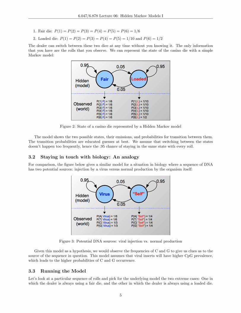
The dealer can switch between these two dice at any time without you knowing it. The only informationthat you have are the rolls that you observe. We can represent the state of the casino die with a simpleMarkov model:
Figure 2: State of a casino die represented by a Hidden Markov model
The model shows the two possible states, their emissions, and probabilities for transition between them.The transition probabilities are educated guesses at best. We assume that switching between the statesdoesn’t happen too frequently, hence the .95 chance of staying in the same state with every roll.
3.2 Staying in touch with biology: An analogy
For comparison, the figure below gives a similar model for a situation in biology where a sequence of DNAhas two potential sources: injection by a virus versus normal production by the organism itself:
Figure 3: Potential DNA sources: viral injection vs. normal production
Given this model as a hypothesis, we would observe the frequencies of C and G to give us clues as to thesource of the sequence in question. This model assumes that viral inserts will have higher CpG prevalence,which leads to the higher probabilities of C and G occurrence.
3.3 Running the Model
Let’s look at a particular sequence of rolls and pick for the underlying model the two extreme cases: One inwhich the dealer is always using a fair die, and the other in which the dealer is always using a loaded die.
5
6.047/6.878 Lecture 06: Hidden Markov Models I
We run the model on each to understand the implications. We’ll build up to introducing HMMs by firsttrying to understand the likelihood calculations from the standpoint of fundamental probability principlesof independence and conditioning.
Figure 4: Running the model: probability of a sequence, given path consists of all fair dice
In the first case, where we assume the dealer is always using a fair die, we calculate the probability asshown in Figure 4. The product term has three components: 1/2 - the probability of starting with the fair
die model, (1/6)10
- the probability of the roll given the fair model (6 possibilities with equal chance), and
lastly (0.95)9
- the transition probabilities that keep us always in the same state.The opposite extreme, where the dealer always uses a loaded die, has a similar calculation, except that
we note a difference in the emission component. This time, 8 of the 10 rolls carry a probability of 1/10based on the assumption of a loaded die underlying model, whiletwo rolls of 6 have a probability of 1/2 ofoccurring. Again we multiply all of these probabilities together according to principles of independence andconditioning. This is shown in Figure 5.
Finally, in order to make sense of the likelihoods, we compare them by calculating a likelihood ratio, asshown in Figure 6.
We find that, it is significantly more likely for the sequence to result from a fair die. Now we step backand ask, does this make sense? Well, of course. Two occurrences of rolling 6 in ten rolls doesn’t seem out ofthe ordinary, so our intuition matches the results of running the model.
3.4 Adding Complexity
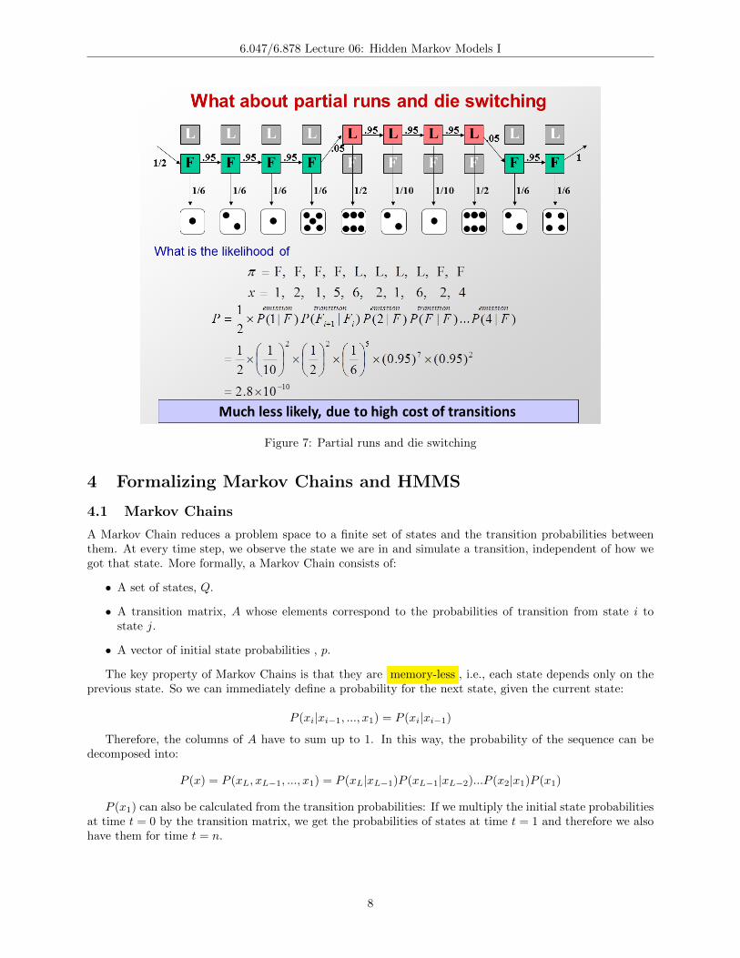
Now imagine the more complex, and interesting, case where the dealer switches the die at some point duringthe sequence. We make a guess at an underlying model based on this premise:
Again, we can calculate the likelihood using fundamental probabilistic methods. From Figure 7, we cansee that, our guessed path is far less likely than the previous two cases. Now, it begins to dawn on us thatwe will need more rigorous techniques for inferring the underlying model. In the above cases we more-or-lessjust guessed at the model, but what we want is a way to systematically derive likely models. Let’s formalizethe models introduced thus far as we continue toward understanding HMM-related techniques.
6
6.047/6.878 Lecture 06: Hidden Markov Models I
Figure 5: Running the model: probability of a sequence, given path consists of all loaded dice
Figure 6: Comparing the two paths: all-Fair vs. all-loaded.
7
6.047/6.878 Lecture 06: Hidden Markov Models I
Figure 7: Partial runs and die switching
4 Formalizing Markov Chains and HMMS
4.1 Markov Chains
A Markov Chain reduces a problem space to a finite set of states and the transition probabilities betweenthem. At every time step, we observe the state we are in and simulate a transition, independent of how wegot that state. More formally, a Markov Chain consists of:
• A set of states, Q.
• A transition matrix, A whose elements correspond to the probabilities of transition from state i tostate j.
• A vector of initial state probabilities , p.
The key property of Markov Chains is that they are memory-less , i.e., each state depends only on theprevious state. So we can immediately define a probability for the next state, given the current state:
P (xi|xi−1, ..., x1) = P (xi|xi−1)
Therefore, the columns of A have to sum up to 1. In this way, the probability of the sequence can bedecomposed into:
P (x) = P (xL, xL−1, ..., x1) = P (xL|xL−1)P (xL−1|xL−2)...P (x2|x1)P (x1)
P (x1) can also be calculated from the transition probabilities: If we multiply the initial state probabilitiesat time t = 0 by the transition matrix, we get the probabilities of states at time t = 1 and therefore we alsohave them for time t = n.
8
6.047/6.878 Lecture 06: Hidden Markov Models I
4.2 Hidden Markov Models
Hidden Markov Models are used as a representation of a problem space in which observations come aboutas a result of states of a system which we are unable to observe directly. These observations, or emissions,result from a particular state based on a set of probabilities. Thus HMMs are Markov Models where thestates are hidden from the observer and instead we have observations generated with certain probabilitiesassociated with each state. These probabilities of observations are known as emission probabilities.
Formally, a Hidden Markov Model consists of the following parameters:
• A series of states, Q.
• A transition matrix, A: For each s, t, in Q the transition probability is: ast = P (xi = t|xi−1 = s)
• A vector of initial state probabilities , p.
• Set of observation symbols, V , for example {A, T, C, G} or, 20 amino-acids or utterances in humanlanguage.
• A matrix of emission probabilities, E: For each s, t, in Q, the emission probability is
esk = P (vk at time t|qt = s)
The key property of memory-less-ness is inherited from Markov Models: the emissions and transitionsare only dependent on the current state and not on the past history.
5 Back to Biology
Now that we have formalized HMMs, we want to use them HMMs in solving some real biological problems.In fact, HMMs are a great tool for gene sequence analysis, because we can look at a sequence of DNA asbeing emitted by a mixture of models. These may include introns, exons, transcription factors, etc. Whilewe may have some sample data that matches models to DNA sequences, in the case that we start freshwith a new piece of DNA, we can use HMMs to ascribe some potential models to the DNA in question. Wewill first introduce a simple example and think about it a bit. Then, we will discuss some applications ofHMM in solving interesting biological questions, before finally describing the HMM techniques that solvethe problems that arise in such a first-attempt/native analysis.
5.1 A simple example: Finding GC-rich regions
Imagine the following scenario: we are trying to find GC rich regions by modeling nucleotide sequences drawnfrom two different distributions: background and promoter. Background regions have uniform distributionof 0.25 for each of A, T, G, C. Promoter regions have probabilities: A: 0.15, T: 0.13, G: 0.30, C: 0.42. Givenone nucleotide observed, we cannot say anything about the region from which it was originated, becauseboth regions could have emited it at different probabilities. We can learn these initial state probabilitiesbased in steady state probabilities. By looking at a sequence, we want to identify which regions originatefrom a background distribution (B) and which regions are from a promoter model (P). It was noted againthat Markov chains are absolutely memory-less, this means that for example if you have lost in a Casino inthe last 7 days, it won’t mean that you would most probably win today. This is also true in the example ofrolling a die where you might have repetitions of a number.
We are given the transition and emission probabilities based on relevant abundance and average lengthof regions where x = vector of observable emissions consisting of symbols from the alphabet {A,T,G,C};π = vector of states in a path (e.g. BPPBP); π∗ = maximum likelihood of generating that path. In ourinterpretation of sequence, the max likelihood path will be found by incorporating all emissions transitionprobabilities (by dynamic programming).
HMMs are generative models, in that an HMM gives the probability of emission given a state (withBayes’ Rule), essentially telling you how likely the state is to generate those sequences. So we can alwaysrun a generative model for transition between states and start anywhere. In Markov Chains, the next state
9
6.047/6.878 Lecture 06: Hidden Markov Models I
Figure 8: HMMS as a generative model for finding GC-rich regions.
will give different outcomes with different probabilities. No matter which the next state is, at that next state,the next symbol will still come out with different probabilities. HMMs are similar: You can pick an initialstate based on initial probability vector. In the example above, you pick B since there are more backgroundthan promoter. Then draw an emission from the P(X—B). Since all are 0.25, you can pick any symbol, forexample G. Given this emission, the probability of the next transition state does not change. So we havetransition to B again is with probability 0.85 and to P with 0.15 so we go with B and so on.
We can compute the probability of one such generation by multiplying the probabilities that the modelmakes exactly the choices we assumed. For the example above we have the probability of three differentpaths computed as in Figures 9, 10, and 11.
Figure 9: Probability of seq, path if all promoter
Now the question is, what path is most likely to generate the given sequence?One brute force approach may be looking at all paths, trying all possibilities, and calculating their joint
probability P (x, π). The sum of probabilities of all the alternatives is 1. For example, if all states arepromoters, P (x, π) = 9.3× 10⁻⁷. If all emissions are Gs, P (x, π) = 4.9× 10⁻⁶. If we have use the mixtureof B’s and P ’s as in Figure 11, P (x, π) = 6.7× 10⁻⁷; which is small because a lot of penalty is paid for thetransitions between B’s and P ’s which are exponential in length of sequence. Usually, if you observe moreG’s, it is more likely to be in the promoter region and if you observe more A and Ts, then it is more likelyto be in the background. But we need something more than just observation to support our belief. In thecoming sections we will see how can we mathematically support our intuition.
10
6.047/6.878 Lecture 06: Hidden Markov Models I
Figure 10: Probability of seq, path if all background
Figure 11: Probability of seq, path sequence if mixed
5.2 Application of HMMs in Biology
HMMs are used in answering many interesting questions. Some biological application of HMMs are summa-rized in the table shown in Figure 12.
6 Algorithmic Settings for HMMs
We use HMMs for three types of operation: scoring, decoding, and learning. We talk about scoringand decoding in this lecture. These operations can happen for a single path or all possible paths. For thesingle path operations, our focus is on discovering the path with maximum probability, the most likely path.However in all paths operations we are interested in a sequence of observations or emissions regardless of itscorresponding paths.
6.1 Scoring
6.1.1 Scoring over a single path
For a single path we define the Scoring problem as follows:
11
6.047/6.878 Lecture 06: Hidden Markov Models I
Figure 12: Some biological applications of HMM
Figure 13: The six algorithmic settings for HMMS
• Input: A sequence of observations x = x1x2 . . . xn generated by an HMM M(Q,A, p, V,E) and a pathof states π = π1π2 . . . πn.
• Output: Joint probability, P (x, π) of observing x if the hidden state sequence is π.
12
6.047/6.878 Lecture 06: Hidden Markov Models I
The single path calculation is essentially the likelihood of observing the given sequence over a particularpath using the following formula:
P (x, π) = P (x|π)P (π)
We have already seen the examples of single path scoring in our Dishonest Casino and GC-rich regionexamples.
6.1.2 Scoring over all paths
We define the all paths version of Scoring problem as follows:
• Input: A sequence of observations x = x1x2 . . . xn generated by an HMM M(Q,A, p, V,E).
• Output: Joint probability, P (x, π) of observing x over all possible hidden state sequences, πs.
we do all operations on all possible paths and states and score the sequence over all paths π using thefollowing formula,
P (x) = ΣπP (x, π)
In this case the score is calculated for just a given sequence of observations or emissions regardless of thepaths. We use this score when we are interested in knowing the likelihood of particular sequence for a givenHMM.
6.2 Decoding
Decoding answers the question: Given some observed sequence, what path gives us the maximum likelihoodof observing this sequence? Formally we define the problem as follows:
• Decoding over a single path:
– Input: A sequence of observations x = x1x2 . . . xN generated by an HMM M(Q,A, p, V,E).
– Output: The most probable path of states, π∗ = π∗1π∗2 . . . π
∗N
• Decoding over all paths:
– Input: A sequence of observations x = x1x2 . . . xN generated by an HMM M(Q,A, p, V,E).
– Output: The path of states, π∗ = π∗1π∗2 . . . π
∗N that contains the most likely states at any time
point.
In this lecture, we will look only at the problem of decoding over a single path. The problem of decodingover all paths will be discussed in the next lecture.
For the single path decoding problem, we can imagine a brute force approach where we calculate thejoint probabilities of a given emission sequence and all possible paths and then pick the path with themaximum joint probability. The problem is - there are exponential number of paths and using such a bruteforce search for the maximum likelihood among all the paths is very time consuming and impractical. Tosolve this problem Dynamic Programming can be used. Let us formulate the problem in the dynamicprogramming approach.
Through decoding we would like to find out the most likely sequence of states based on the observation.For the decoding operation, the model parameters eis (the emission probabilities given their states) andaijs, (the state transition probabilities) are given. Also, the sequence of emissions x is given. The goal isto find the sequence of hidden states, π∗, which maximizes the joint probability of a given emission and itspath P (x, π), i.e.,
π∗ = arg maxπP (x, π)
Given the emitted sequence x we can evaluate any path through hidden states. However we are lookingfor the best path. We start by looking for the optimal substructure of this problem.
For a best path, we can say that, the best path through a given state must contain within it the following:
13
6.047/6.878 Lecture 06: Hidden Markov Models I
• Best path to previous state
• Best transition from previous state to this state
• Best path to the end state
Therefore the best path can be obtained based on the best path of the previous states, i.e., we can find arecurrence for the best path. The Viterbi algorithm, a dynamic programming algorithm, is commonly usedto obtain the best path.
6.2.1 Most probable state path: the Viterbi algorithm
Suppose, the probability vk(i), of the most likely path ending at state k at position (or time instance) i inthe path (which can be shown as πi = k) is known for all the states k. Then we can compute this probabilityat time i+ 1, as follows:
vl(i+ 1) = el(xi+1)maxk(aklvk(i))
The most probable path π∗ or the maximum P (x, π) can be found recursively. Assuming we knowvj(i− 1), the score of the maximum path up to time i− 1, now we need to increase the computation for thenext time step. The new maximum score path for each state depends on
• the maximum score of the previous states
• the penalty of transition to the new states (transition probability), and
• the emission probability.
In other words, the new maximum score for a particular state at time i is the one that maximizes thetransition of all possible previous states to that particular state (the penalty of transition multiplied by theirmaximum previous scores multiplied by emission probability at the current time).
All sequences have to start in state 0 (the begin state). By keeping pointers backwards, the actual statesequence can be found by backtracking. The solution of this Dynamic Programming problem is very similarto the alignment algorithms that we studied in previous lectures.
The steps of the Viterbi algorithm ?? are summarized below:
1. Initialization (i = 0): v0(0) = 1, vk(0) = 0 for k > 0.
As we can see in Figure 14, we fill the matrix from left to right and trace back. Each position in thematrix has K states to consider and there are KN cells in the matrix, so, the required computation timeis O(K2N) and the required space is O(KN) to remember the pointers. Note that, the running time hasreduced from exponential to polynomial.
6.3 Evaluation
Evaluation is about answering the question: How well does our model of the world capture the actual world?Given a sequence x, many paths can generate this sequence. The question is how likely is the sequence, giventhe entire model? In other words, is this a good model? Or, how well the model does capture the exactcharacteristics of a particular sequence? We use evaluation operation of HMMs to answer these questions.With evaluation we can compare the models.
Let us formally define the Evaluation problem first.
• Input: A sequence of observations x = x1x2 . . . xN and an HMM M(Q,A, p, V,E).
• Output: The probability that x was generated by M summed over all paths.
14
6.047/6.878 Lecture 06: Hidden Markov Models I
Figure 14: The Viterbi algorithm
We know that, if we are given an HMM, we can generate a sequence of length n easily using the followingsteps:
• Start at state π1 according to probability a0π1(obtained using vector, p).
• Emit letter x1 according to emission probability eπ1(x1).
• Go to state π2 according to the transition probability aπ1|π2
• Keep doing this until emit xN .
Thus we can emit any sequence and calculate its likelihood. However, many state sequence can emit thesame x. Then, how do we calculate the total probability of generating a given x over all paths? That is, ourgoal is to obtain the following probability:
P (x|M) = P (x) =∑π
P (x, π) =∑π
P (x|π)P (π)
The challenge of obtaining this probability is there are too many paths (exponential number of paths).Each path has an associated probability. Some paths are more likely, some are less likely, and we need tosum them up all. One approach may be using just the Viterbi path and ignoring the others. We alreadyhave shown how to obtain the Viterbi path. But its probability is very small; it is just a small fraction of theprobability mass of all possible paths. It is a good approximation only if it has high probability density. Inother cases, it will give us an inaccurate approximation. So, the correct approach calculating the exact sumiteratively by using dynamic programming. The algorithm that does this is known as Forward Algorithm.
6.3.1 The Forward Algorithm
First we derive the formula for forward probability f(i).
From Figure 15, it can be seen that, the Forward algorithm is very similar to the Viterbi algorithm. Inthe Forward algorithm, summation is used instead of maximization. Here we can reuse computations of theprevious problem including penalty of emissions, penalty of transitions and sums of previous states. Therequired computation time is O(K2N) and the required space is O(KN). The drawback of this algorithm isthat in practice taking the sum of logs is difficult; therefore approximations and scaling of probabilities areused instead.
16
6.047/6.878 Lecture 06: Hidden Markov Models I
7 An Interesting Question: Can We Incorporate Memory in OurModel?
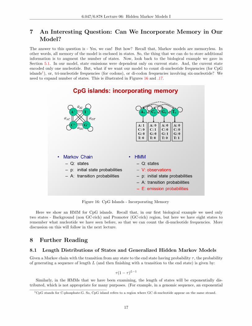
The answer to this question is - Yes, we can! But how? Recall that, Markov models are memoryless. Inother words, all memory of the model is enclosed in states. So, the thing that we can do to store additionalinformation is to augment the number of states. Now, look back to the biological example we gave inSection 5.1. In our model, state emissions were dependent only on current state. And, the current stateencoded only one nucleotide. But, what if we want our model to count di-nucleotide frequencies (for CpGislands1), or, tri-nucleotide frequencies (for codons), or di-codon frequencies involving six-nucleotide? Weneed to expand number of states. This is illustrated in Figures 16 and .17.
Figure 16: CpG Islands - Incorporating Memory
Here we show an HMM for CpG islands. Recall that, in our first biological example we used onlytwo states - Background (non GC-rich) and Promoter (GC-rich) region, but here we have eight states toremember what nucleotide we have seen before, so that we can count the di-nucleotide frequencies. Morediscussion on this will follow in the next lecture.
8 Further Reading
8.1 Length Distributions of States and Generalized Hidden Markov Models
Given a Markov chain with the transition from any state to the end state having probability τ , the probabilityof generating a sequence of length L (and then finishing with a transition to the end state) is given by:
τ(1− τ)L−1
Similarly, in the HMMs that we have been examining, the length of states will be exponentially dis-tributed, which is not appropriate for many purposes. (For example, in a genomic sequence, an exponential
1CpG stands for C-phosphate-G. So, CpG island refers to a region where GC di-nucleotide appear on the same strand.
17
6.047/6.878 Lecture 06: Hidden Markov Models I
Figure 17: Counting Nucleotide Transitions
distribution does not accurately capture the lengths of genes, exons, introns, etc). How can we construct amodel that does not output state sequences with an exponential distribution of lengths? Suppose we wantto make sure that our sequence has length exactly 5? We might construct a sequence of five states withonly a single path permitted by transition probabilities. If we include a self loop in one of the states, we willoutput sequences of minimum length 5, with longer sequences exponentially distributed. Suppose we havea chain of n states, with all chains starting with state π1 and transitioning to an end state after πn. Alsoassume that the transition probability between state πi and πi+1 is 1−p, while the self transition probabilityof state πi is p. The probability that a sequence generated by this Markov chain has length L is given by:(
L− 1
n− 1
)pL−n(1− p)n
This is called the negative binomial distribution.More generally, we can adapt HMMs to produce output sequences of arbitrary length. In a Generalized
Hidden Markov Model [1] (also known as a hidden semi-Markov model), the output of each state is a stringof symbols, rather than an individual symbol. The length as well as content of this output string can bechosen based on a probability distribution. Many gene finding tools are based on generalized hidden Markovmodels.
8.2 Conditional random fields
Conditional random field model is an alternative to HMMs. It is a discriminative undirected probabilisticgraphical model. It is used to encode known relationships between observations and construct consistentinterpretations. It is often used for labeling or parsing of sequential data. It is widely used in gene finding.The following resources can be helpful in order to learn more about CRFs:
• Lecture on Conditional Random Fields from Probabilistic Graphical Models course: https://class.coursera.org/pgm/lecture/preview/33. For background, you might also want to watch the twoprevious segments, on pairwise Markov networks and general Gibbs distributions.