Distribution Category: Liquid Metal Fast Breeder Reactors (UC-79) ANL-80-97 ARGONNE NATIONAL LABORATORY 9700 South Cass Avenue Argonne, Illinois 60439 THERMAL-PERFORMANCE STUDY OF LIQUID METAL FAST BREEDER REACTOR INSULATION by Kelvin K. Shiu September 1980 DISCLAIMER Based on a thesis submitted to the Graduate School of the University of Illinois-w-Urbana in partial fulfillment of requirements for the degree of Doctor of Philosophy in Nuclear Engineering
Transcript
Distribution Category:
Liquid Metal FastBreeder Reactors (UC-79)
ANL-80-97
ARGONNE NATIONAL LABORATORY9700 South Cass Avenue
Argonne, Illinois 60439
THERMAL-PERFORMANCE STUDY OFLIQUID METAL FAST BREEDER REACTOR INSULATION
by
Kelvin K. Shiu
September 1980
DISCLAIMER
Based on a thesis submitted to theGraduate School of the University of Illinois-w-Urbana
in partial fulfillment ofrequirements for the degree of
101. Temperature Distribution of 24 Screen Plates Wetted with 8 in.(203 mm) of Sodium, Hot-face Temperature at 857F (458 C)........ 111
102. Temperature Distribution of 24 Screen Plates Wetted with 8 in.
(203 mm) of Sodium, Hot-face Temperature at 690F (366*C)..........111
103. Temperature Distribution of 24 Screen Plates Wetted with 8 in.
(203 mm) of Sodium, Hot-face Temperature at 520F (271C)..........112
104. Temperature Distribution of 24 Screen Plates Wetted with 8 in.
(203 mm) of Sodium, Oxidized, Hot-face Temperature at 448F(231 C).......................................................... 112
105. Temperature Distribution of 24 Screen Plates Wetted with 8 in.
(203 mm) of Sodium, Oxidized, Hot-face Temperature at 615 F(324 C).......................................................... 112
106. Temperature Distribution of 24 Screen Plates Wetted with 8 in.(203 mm) of Sodium, Oxidized, Hot-face Temperature at 820F(438C).................................................................... 113
107. Sodium Oxide Deposits on Plate................................... 113
108. Exaple of Sodium Oxide Deposits on First Few Screens............ 114
11
LIST OF FIGURES
No. Title Page
109. Example of Sodium Oxide Deposits on Last Few Screens..............114
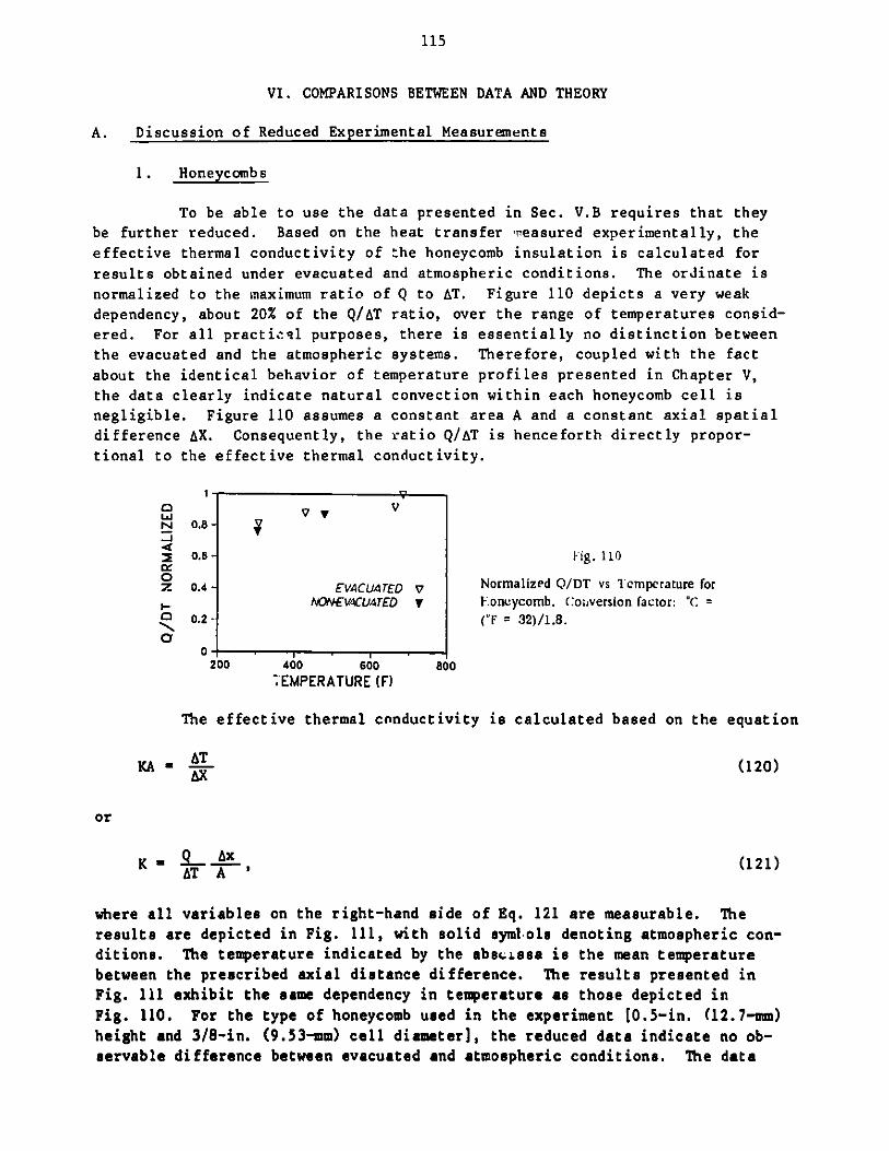
110. Normalized Q/DT vs Temperature for Honeycomb......................115
111. Effective Thermal Conductivity vs Temperature for Honeycomb........116
112. Normalized Q/DT vs Temperature for 12 Multiplates.................116113. Effective Thermal Conductivity vs Temperature for 12 Multiplates. 117114. Normalized Q/DT vs Temperature for 24 Multiplates.................118115. Effective Thermal Conductivity vs Temperature for 24 Multiplates. 118116. Normalized Q/DT vs Temperature for 12 Screen Plates.............. 119117. Effective Thermal Conductivity vs Temperature for 12 screen
120. Effective Thermal Conductivity vs Temperature for 24 Screen
Plates with Sodium and Sodium O xide.............................. 122
121. Effective Thermal Conductivity vs Temperature for Screen Plates,
Composite Insulation by Lemercier et al. ......................... 125
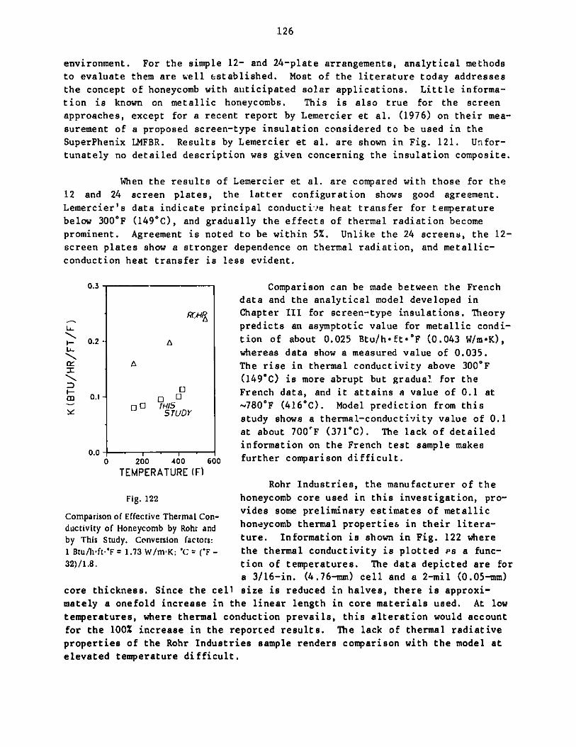
122. Comparison of Effective Ther-nal Conductivity of Honeycomb by Rohrand by This Study................................................. 126
C.1. Insulated Thermocouple Attached to Massive Solid..................135
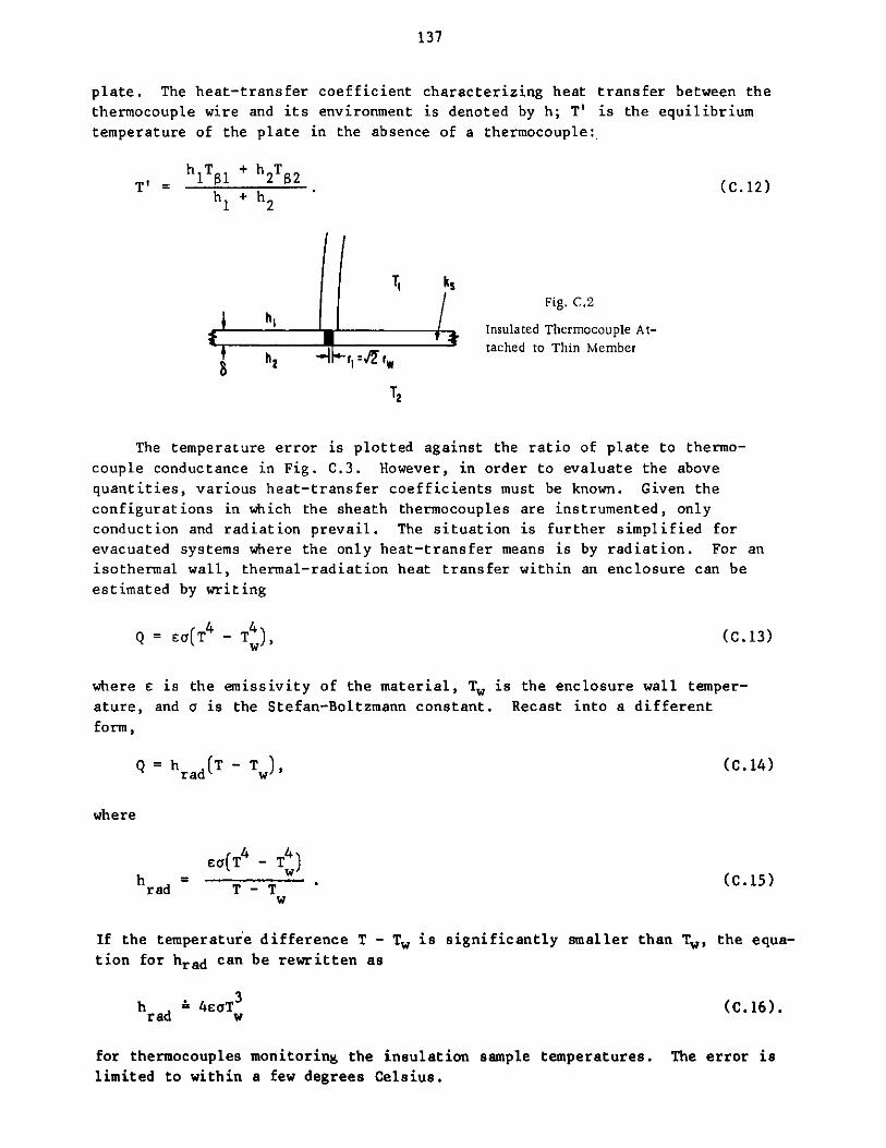
C.2. Insulated Thermocouple Attached to Thin Member....................137
C.3. Temperature Errors vs Thermocouple Conductance....................138
E.1. Derivation of e + T = 1.......................................... 140
E.2. Derivation of e + p + T = 1...................................... 140
E.3. Total Thermal Resistance between Two P ates Separated by a Non-
reflective and Nonopaque Medium.................................. 141
E.4. Total Thermal Resistance between a Black Surface and Its Adjacent
Nonreflective and Nonopaque Medium................................141
E.5. Total Thermal Resistance between Two Plates Separated by a Re-flective, Transparent, and Emissive Medium........................142
12
LIST OF TABLES
No. Title Page
I. Sunmary of French Screen-type Insulation..........................28
I I. Values of Ni as a Function of Wave Nunber a, from Catton (1966) . 43
III. Fabrication and Inspection Requirements for Test Vessel......... 72
13
THERMAL-PERFORMANCE STUDY OF
LIQUID METAL FAST BREEDER REACTOR INSULATION
by
Kelvin K. Shiu
ABSTRACT
Three types of metallic thermal insulation were
investigated analytically and experimentally: multilayer
reflective plates, multilayer honeycomb composite, and
multilayer screens. Each type was subjected to evacuated and
nonevacuated conditions, where thermal measurements were made
to determine thermal-physical characteristics. A variation of
the separation distance between adjacent reflective plates of
multilayer reflective plates and multilayer screen insulation
was also experimentally studied to reveal its significance.
One configuration of the multilayer screen insulation was
further selected to be examined in sodium and sodium oxide
environments. The emissivity of Type 304 stainless steel used
in comprising the insulation was measured by employing
infrared technology.
A comprehensive model was developed to describe the
different proposed types of thermal insulation. Various modes
of heat transfer inherent in each type of insulation were
addressed and their relative importance compared. Provision
was also made in the model to allow accurate simulation of
possible sodium and sodium oxide contamination of the
insulation. The thermal-radiation contribution to heat
transfer in the temperature range of interest for LMFBR's was
found to be moderate, and the suppression of natural
convection within the insulation was vital in preserving its
insulating properties. Experimental data were compared with
the model and other published results. Moreover, the threeproposed test samples were assessed and compared under various
conditions as .viable LMFBR thermal insulations.
I. INTRODUCTION
Motivated by the concepts of producing more fissionable materials than it
consumes and of better heat-transfer capabilities from fuel to coolant, the
Liquid Metal Fast Breeder Reactor (LMFBR) was conceived in the middle 1940's.
Because of the inherent characteristic that a nuclear reactor's power output is
primarily limited by the ability to transfer heat away from the fuel, liquid
metals with their superb heat-transfer characteristics were suggested for use
14
as reactor coolants. Both sodium and a mixture of sodium and potassium (NaK)
were two liquid metals that received a great deal of attention in the early
development of the LMFBR. However, when more became known about these liquid
metals, particularly their fire-hazard potential and NaK's corrosive properties,
Nak was rendered less attractive than sodium as a reactor coolant, and sodiumis being used almost exclusively in today's LMFBR systems. Another major at-
traction of sodium in an LMFBR is its by neutron-absorption cross section at
high energies. This enhances the reactor's ability to produce more fuel thanit consumes if fertile fuel blanket assemblies are placed around the reactor
core to capture this breeding capability.
Various design approaches of the primary system and the reactor vessel
were proposed. Presently, all IMFBR's can be categorized as either pool or
loop types. The pool-type design can be characterized by a large reactor ves-
sel within which is contained the primary heat-transport system, which com-
prises both the primary puaps and the intermediate heat exchangers. These
components are immersed in a pool of sodium covering the reactor core, and
thus, the name pooi-type LMFBR. For a loop-type reactor, the components are
located outside the reactor vessel and are interconnected by piping forming
"loops" to allow sodium to flow to and from each component. Because of this
major difference in component locations, the loop reactor requires a smaller-
diameter reactor vessel. For a small power reactor, e.g., Clinch River Breeder
Reactor (CRBR) (300 MWt), the closure of the reactor vessel comprises only
rotating plugs, whereas, for a similar power-size pool reactor, the closure
consists of the rotating plugs as well as a shield deck.
In the recent designs of a commercial-size plant (1200 MWe), the diameterof the pool-type IMFBR reactor vessel is 60-80 ft (18.3-24.4 m); its loop-type
counterpart is about 40 ft (12.2 m). Moreover, the closure head of a loop-type
reactor vessel is proposed to consist of the rotating plugs and a shield deck.
There are indications that the use of a large reactor vessel might mitigateeffects of events such as core-disruptive accidents. Besides the safety fea-
tures, the large-diameter vessel is also favored because, with the large sodiuminventory inside, it provides a means to reduce thermal transient effects.
There is increasing evidence that the large reactor vessel will be used for
loop-type LMFBR's. Both General Electric and Westinghouse, in their loopPrototype Large Breeder Reactor (PLBR) conceptual designs, proposed 40-ft
(12.2-m)-dia reactor vessels.
Various deck designs were proposed, and some of them were built. Experi-
mental Breeder Reactor II (EBR-II) and Phenix use the integral-deck approach,
where the closure deck and the vessel wall form an integral member, subjecting
the closure to elevated temperature. Thermal insulation is placed on the out-
side of the closure to prevent heat losses. The advantage of an integral deckstems from its ability to form a fairly tight boundary to contain sodium aero-sols transport. The requirement imposed on the thermal insulation are also
less stringent. However, operating experience indicates certain unattractive
features of this approach, one of which is that thermal-transient effects
15
resulted in significant stresses on the integral member. This has prompted the
French reactor designers to explore an alternative approach, namely, the cold-
deck design, in which the shield deck is maintained at only a slightly elevated
temperature [~-50 F (66 C)]. Instead of a complete steel structure, a web
approach filled with high-density concrete is suggested. The load of the deck
is taken up by the web structure, and the concrete is used only for gamma-
shielding purposes. To maintain the required temperature level on the deck
structure, thermal insulation is used on the underside of the deck, where it is
exposed to sodium aerosols. Furthermore, a cooling system is also implemented
within the deck structure to ensure desired temperature levels under all oper-
ating conditions. As noted earlier, the closure of small loop reactors com-
prises only the rotating plugs, and because of the ability of these plugs
to allow free expansion, thermal-insulation requirements become less stringent.
However, a situation similar to the pool reactor is encountered when a large
loop reactor is considered where the shield-deck requirements are comparable.
Due to the similarities between both the large loop and pool decks, from
now on only the pool will be used as an example for illustrative purposes, in
fact, the arguments and discussion also apply to large loop reactors. Because
of the enormous size of the deck, both axially and radially, any significant
variations in temperature distributions within the structure would impose unwar-
ranted stresses upon the deck structure, causing the structure to bow. Conse-
quently, if unchecked, this could lead to disruption of fuel handling and of
reactor shutdown controls. The amount of heat transferred through the deck
structure and the concrete should always be maintained within an acceptable low
level. Thus, a reliable and safe operation of the deck structure becomes the
criterion by which performance of an insulation is evaluated.
Besides the above constraints, there are additional requirements that an
acceptable thermal insulation must satisfy. First, the insulation cannot in any
way interact, or physically or chemically degrade, when it comes into contact
with sodium. If the insulatLon has to be used on the underside of the deck,access for inspection, repair, or maintenance will be severely limited. Hence,
it must be reliable throughout the lifetime (~30-40 yr) of the plant without
scheduled maintenance or inspection. Moreover, since the insulation is exposedto high-temperature sodium ~950 F (5100C), large quantities of aerosols are
expected to be transported from the hot sodium surface to the colder surfacesof the insulation on which they will condense. This, in effect, will reduce
the insulating capability enormously over a long period of time. The insula-
tion should tL;erefore exhibit the inherent characteristic of high resistance to
aerosol penetration. For large reactors, sodium sloshing caused by seismicdisturbances and impulses, or any other safety-related hypothetical design
events, could impose on the insulation tremendous impacts to which it is notnormally subjected. Hence, it must also be able to sustain the aforementionedevents without compromising its integrity.
In view of the above requirements, many types of commonly considered ther-
mal insulation can be eliminated, for example, fiber glass or calcium silicate,
16
since these materials are incompatible with sodium. Most refractory materials,
due to their ceramic nature, cannot be considered either. Some metallic re-
flective foils, a few mils thick, can indeed sustain long time exposure to
sodium, and yet their lack of physical strength poses support arid seismic prob-
lems. Layers of metallic plates spaced a certain distance apart were proposed
to be used a, PLBR insulations. The British use this approach in their Proto-
type Fast Reactor (FFR). The advantage of the multiplates is that they are
simple and inexpensive.
A different kind of insulation is proposed to be used by the French in
their SuperPhenix (1200-MWe) commerical-size plant. It comprises layers of
metallic plates, each separated by layers of screens. Other more exotic types
of insulation were also suggested, e.g., honeycomb composites. All these are
to be made of either Type 304 or 316 stainless steel, whose compatibility with
sodium is well known. Each of them provides its own uniqueness in realizing
the objectives as LMFBR insulation. Certainly, other kinds of insulation might
lend themselves to be possible thermal insulation for an LMFBR system. This
study, however, is confined to discussion of the above three types.
Among the types of insulation proposed, the multiplate approach is the
most studied one. However, the effects on thermal properties for various num-
bers of layers need to be examined. The Freinch-type screen insulation, on the
other hand, is the least known. To effectively use the screen-type insulation,
various aspects of heat-transfer processes will have to be identified and under-
stood. Metallic honeycomb has been widely applied in many areas, but not as a
thermal insulation. Its thermal characteristics as a function of temperature
require further investigation. The presence of sodium and/or sodium oxide on
any of these types of insulation may substantially affect their thermal perfor-
mance. Little information is available on these long-term effects. Therefore,
it is important to have experimental results using sodium to simulate condi-
tions in which insulation performance in a reactor can be studied. All theseconstitute different vital areas in which analytical and experimental studies
would lead to increased confidence in plant design and reliability and form thebasis for this study.
II. LITERATURE SURVEY
A. Design Approaches, Proposed Concepts, and Factors Affecting Insulation
Performance in LMFBR Systems
Since the mid 1940's, different types of fast reactors were built, many
having very small cores as well as small thermal outputs. Clementine, the
first fast reactor developed at Los Alamos Scientific Laboratory, had a core
5.9 in. (150 mm) in diameter and 5.5 in. (140 mm) high, completely surrounded
by steel. This was reported by Jurney (1954) and Arnold (1953). Later, reac-
tors with similar core sizes but various core designs were built, e.g., USSR-
BRS, EBR-II, and homogeneous-core reactors LAMPRE-I and -II. By the late
17
1950's, the United Kingdom built Dounreay with a 21-in. (533.4-mm)-dia, 21-in.
(533.4-mm)-high core. All the reactor closures aforementioned had only very
simple dome structures. Also, because of their reduced physical sizes, thermal-
related problems were only of a minor nature. All these systems were cooled by
liquid ntals, e.g., sodium, mercury, or NaK.
By the 1960's, the United States embarked on a nuclear-reactor program in
which two different design concepts were studied, reviewed, analyzed and
finally built. They were the Experimental Breeder Reactor II (EBR-II) and the
Fermi Reactor. These two design concepts represented a marked difference in
design approaches from then until the present. A major characteristic of
EBR-II is that, unlike its predecessors, both its primary pumps and its inter-
mediate heat exchangers are placed within the reactor vessel. Despite the fact
that the core of EB2-II is almost six times smaller than the one of Fermi, the
reactor vessel of EBR-II is 26 ft (7.93 m) in diameter versus 14.5 ft (4.42 m)
for the Fermi Reactor. As can be seen from Fig. 1, the closure of the Fermi
Reactor essentially comprises the fuel-handling and -control mechanisms that
form an integral part of the closure. Figure 2 shows an elevation view of
the primary tank of EBR-II. The cover is made of a carbon-steel plate con-
nected to the primary tank wall, forming a boundary for the sodium aerosols.
Conventional thermal insulation is placed on the top side of this carbon-steel
plate to provide the necessary thermal gradient for the upper structure.
Later, the French built the Phenix Reactor, in which major resemblances
with EBR-II can be noted. Among the similarities is the reactor cover, as can
be seen in Fig. 3. The name pool-type reactor is adopted to describe such a
large reactor vessel within which is contained the primary heat-transport
system. At about the same time, the United Kingdom constructed the Prototype
Fast Reactor (PFR), which is also a pool type. However, instead of an integral
deck, the British chose to place the thermal insulation below the deck, thus
enabling a low-temperature closure structure, as seen in Fig. 4. Only recently,
the French started construction on the full-size (1200-MWe) demonstration plant,
which is also a pool reactor with a reactor vessel about 70 ft (21.3 m) in diam-
eter. Contrary to their Phenix design, they adopted a PFR-type deck approach,
shown in Fig. 5, in which thermal insulation is required below the closure
structure. During the last few years, other pool-type design concepts have been
proposed and studied, and most of them favor the cold-deck underside-insulation
approach. Some of these concepts are shown in Figs 6 and 7.
An alternative approach, in which the primary heat-transport system is
located outside the reactor vessel, is conveniently called the loop concept.
The Fast Fluxc Test Facility (FFTF), shown in Fig. 8, is a design of this kind
that is being built in the United States. The West German SNR-300 (Fig. 9) and
the Japanese Monju (Fig. 10), both of which are loop reactors, are also being
constructed. Despite the fact that these reactors are designed by different
countries, the closures of both reactor vessels are extremely similar. For the
pool reactors, the closure consists of the rotating plugs and the shield deck,
18
Offset HandlingHolddown Drive Mechanism
Transfer RotorDrive Mechanism
Plug Drive Mechanism
Deck Structure
- --- - Rotating Plug!III ' I I I IContai nur
I! i i I Normal Operation)
-Sodium LevelExit Port -(Refueling)
Offset II"
HandlingMechansm
SRotating-I C Upper ~30" Outlet
Plug Reactor Holddown
Thermal Column
Shield D sAlignment Spider
Exit Port, -tHolddown Plate
6" Radial BlanketInlet
- 14" Core Inlet
Rotor I oreSupport Support Plates
Assembly ... Radial Blanket
Saseby -I - - Thermal ShieldTransfer Pot ITransfer ~
RotorContainer Radial Blanket
Prmr ___ Inlet Plenum
Shield Tonk mCore
Vessel Inlet Plenum
FlexplateSupports
Radial Blanket Inlet Manifold Support Plate Support Structure
Fig. 1. Cross Section of Fermi Reactor. Conversion factor: 1 in. = 25.4 mm.
19
--
Fig. 2. Elevation View of EBR-1I
-F I
+ at ,
j!~~ ~ it t,
A CONTROL ROD MECHANISM
B FUEL TRANSFER ARM CONTROL
C. INTERMEDIATE HEAT EXCHANGER (6)
D. PRIMARY CIRCULATION PUMP (3)
E. FUEL TRANSFER ARM
F ROTATING PLUG
G. SURROUNDING NEUTRON SHIELDING
H TOP NEUTRON SHIELDING
J. CORE
K. 21 SUSPENSION POINTS
L. MAIN TANK
M. LEAK TANK
N. SAFETY TANK
0. CONICAL SUPPORT COLLAR FOR REACTOR
Fig. 3. Elevation View of Phenix Reactor
SUBASSEMBL-FUEL UNLOADING TRANSFER COFFIN
CUNTROL ROO DRIVES (11
- ROTATING PLLGS -
STORAGE BASKET
PRIMARY - -
PRIMARY A. LA;Y PIMP: PRIMARY SODIUM PUMP(:)
REAC TOR I
BLAST SHIELL SArETY ROOSI)
BIOLOGICAL .E LC --
SIlR BAFFLE
I
-
20
Rotating Shield - PumpReactor Roof
Sodium
Insulation Sodiu
Intermediate Pump
Neat Exchanger
Pnimory Vessel
Look Jacket - -j Valve
Core NeutrCoreReactor J1 cat - -
- -&Beed
--- Insulat
D& SDiagrid sup'Structure- -
Fig. 4. elevation View of Prototype Fast Reactor
METALLIC -. ROTATING CONTROL-ROD FUEL IRAINSULATION PLUG VES
\ -t 1 1
- ARGON SPACE iNSTI TREE - - - -"I iHOT
(I POOL t T
EMERGENCY I IHX 1- 4COOLING SYSTEM
I PUMP
FUEL -TRANSFER RAMP
STEFASSviMdLIES
DIAGRID -- -
CORE CATCHER--
NSFER GRIPPER
CORE
COLD POOLAREAS
Fig. 5. Elevation View of SuperPhenix Reactor
n Shield
lion
m Levels
21
W WIII , PLUG -O A lUG L
I"- 0 pPLUG : "
esL I 4, CCCOLLWGDCCI- - - -( wL Pump WILL
.. , - C Duct
. l L 01a WILL
-ntal - (C~WO O*,~P
-~ o r '-- 40.
I' _AAA P1W -1a w uLO
l -rr t - " " -' 'M
'u1.- - :U. C MP
-I A W( I -Pit-
wLL rW S j - I-- 1AL O ouW WASM( LS
rp.«-x ,"1c t rua W 14 CO W tt
IL d r'- mnulstss SWS(LOI-
-a sM 1isnt-
-- - sECaO /v 0- ---ti
:I I- - an ua n lAUT,!r LIII SA W___ __ «I UCLL WOL
whereas the loop-reactor closure consists of only rotating plugs. Recent PLBR
studies for a commercial-size loop-type LMFBR show that larger reactor vessels,
in the order of 40 ft (12.2 m), are favored. This will result in a reactorvessel design comparable to the pool concept, in which both the rotating plugsand the shield deck make up the closure of the vessel (information primarily
obtained from reports by A. Amorosi et al. and other internal reports at ANL).
A principal reason why thermal insulation has been such an important area
in which detailed information is needed, is because, previously, for loop-
reactor closures, thermal gradients and thermal expansions can easily be accom-
modated by free-end support arrangements. Furthermore, the reduced sizes of
earlier generations of reactors serve to diminish such difficulties; there-
fore, the requirements of thermal insulations are much less critical. The
integral-deck or hot-roof approach for the first generation of pool reactors
poses unusual thermal-stress and thermal-stripping problems during normal oper-
ating conditions. These difficulties are further amplified during transients
and variations in primary-pump speed condit-ons. Therefore, coupled with the
earlier operating experiences and the fact that reactor-vessel diameters are
progressing to larger dimensions, "under-roof" thermal insulation has become
increasingly vital and essential for building a reliable LMFBR system.
Only recently has the topic of thermal insulation begun to receive some
limited attention. Because of the location at which the insulation will be
placed, certain unique situations will have to be considered. In addition to
the requirements outlined in Chapter I for thermal insulation, a recent report
by Collins (1978) also specifies that adequate flexibility and structural com-
pliance to accommodate normal thermal dilatation between the insulation, the
shield deck, and components that penetrate the shield and insulation are needed
to avoid damaging thermal stresses. The insulation must retain its integrity
during and after design seismic events, including forces from structural accel-
erations and inertial sloshing of sodium. These become the basic requirements
used to evaluate any proposed insulation.
Different materials have been examined for their compatibility with sodium
dAring various nuclear-reactor-related studies, e.g., Balkwill (1974) and Fink
(1976). Their conclusions indicate that because of sodium's extraordinary
reducing properties, almost all conventional thermal insulation will not be
compatible. Some react exothermically with sodium; others react violently.
Generally, materials containing silicate react with sodium. Some metals, e.g.,
copper or iron, are also susceptible to sodium reaction, as reported by
McKisson (1970). Only a few metallic materials proved to be attractive, and
among them are Types 304 and 316 stainless steel. Low thermal conductivity,
comparative low cost, and wide availability render stainless steel of both
kinds to be very promising insulation material.
In most proposed LMFBR systems, normal operating sodium temperature is
950-1000 F. Figure 11 shows that at such temperatures sodium vapor pressure is
25
quite substantial. This imp' s that large quantities of sodium-vapor aerosols
will be created and, by mea of diffusion and convection, the aerosols will be
transported from the pool st ace up to the insulation, where condensation and
deposition will take place, as seen from Fig. 12. Any extended penetration of
sodium aerosols into the insulation will almost certainly reduce its insulatingeffectiveness. Perhaps a similar detrimental effect as a consequence of aero-
sol transport is the oxidation of the sodium into sodium oxide or super oxide,which exhibits a very high thermal-emissivity value. Aside from the thermaldegradation caused by increased thermal radiation and conduction heat transfer,
both sodium and its various oxides could also prevent proper operation of equip-
ment, e.g., the rotating-plug seals of EBR-II reported by Copper (1969) andcontrol-rod mechanisms and rotating plugs of Phenix reported by Delisle (1977).
Therefore, in addition to the requirements stated earlier, the thermal insula-
tion should also be able to provide some form of vapor-transport barrier to
reduce the deposits of sodium and sodium oxides on the shield deck as well as
Within the last few years, various kinds of metallic thermal insulation
have been proposed for these LMFBR systems. Despite the unique requirements
presented in Sec. A above, different ideas originally conceived for other in-
dustrial applications are examined and modified. One of these is the multi-
layer insulation concept. Other ideas of encapsulating conventional thermal
insulation are also explored.
Thermal baffles, which are essentially
have been widely used as thermal insulation
development of liquid-metal-cooled reactors,
in Hallum and SRE. Figure 13 shows the find
'n the two reactors. The white deposits are
layers of reflective materials,
for a long time. During the early
a similar concept was used, e.g.,
of multi'ayer metallic plates used
sodium and sodium oxides. During
ce -
ling
I.
aerosol
1
I
vapor pressure(10 ;/cm2 )
310
~ I
C I
II~1
10-6
10
500
itJ
f:i
27
the 1960's the application of multilayer reflective-radiation shield was further
perfected by the aerospace industry. Various parametric and thermal character-
istic studies were performed. The work is summarized in the NASA report by
Glaser et al. (1967). However, these types of insulation were developed for
lightweight and compact applications, and mechan;-al strength was not a major
concern. Hence, metallic foils, whose thickness .as in the order of a thou-
sandth of an inch or hundredth of a millimeter, were commonly used. Rarely
would these insulations exceed an overall thickness of a few inches (200 mm).
Due to the lack of strength of the reflective shields, a variety of spacer
materials was proposed to remedy the direct contact problem between foils.
Paquin (1968) proposed the use of high-purity refractory oxides as spacers.
Some of the more common ones are silk, Mylar, dimpled sheets, paper, and mica.
They are chosen because of their poor thermal conductivities and, thus, con-
tribute in reducing conduction heat transfer from one layer to another.
Fig. 13. Multilayer Plates after Exposure to Sodium
Plain multiple-layer reflective plates have been proposed by Atomics Inter-
national and Westinghouse to be used in their PLBR loop systems. This type of
insulation is actually being used inside the British PF\ system. Nevertheless,reservations concerning the integrity of the insulation over long time exposure
to sodium aerosols can be demonstrated by the French revolutionary approach of
28
a patented concept by Lemercier (1973) in which metallic screens are added
between each pair of reflective shields. Detailed information on the design of
this type of insulation is not available. It is unclear whether one of the
patent concepts or a modified version of them will actually be used in the
SuperPhenix Reactor. Limited sources indicate that screen-filled multilayer
reflective insulation will be used. Both French patents describe some sort of
encapsulation with a stainless steel container sealed by capillary effects.
Different screen-wire dimensions and mesh sizes have been presented. A paper
presented in 1976 by one of the inventors, Lemercier, reported the conclusions
of a testing program of this type of insulation; but variance is noted on such
critical dimensions of the insulation as screen-wire size, mesh size, and thick-
ness when compared to the patents. A summary is presented in Table I. Recently,
insulation of layers of screens and layers of plates was proposed by General
Electric to be used in their PLBR pool design.
TABLE 1. Summary of French Screen-type Insulation
Patent Patent Lemercier
No. 73 23338 No. 73 23339 (1976)
Wire diameter
(mm) 0.4 0.4 20.6a
Wire mesh(mm) 4 NA NA
Overall
thickness
(mm) NA 120 NA
aWire gauge screen.
Other ideas of an acceptable thermal insulation have also been suggested,
one of which is the honeycomb approach, which will receive an extensive treat-
ment here. The purpose of using honeycomb-type material in different applica-
tions varies widely from structural strength, to noise control, to solar
collectors. Metallic honeycombs are widely used in the aircraft industry to
build wings, fuselages, and other parts of planes. Incidentally, at Argonne
National Laboratory, the idea was conceived that if face sheets, which were es-
sentially reflective thermal-radiation shields, could be placed between a
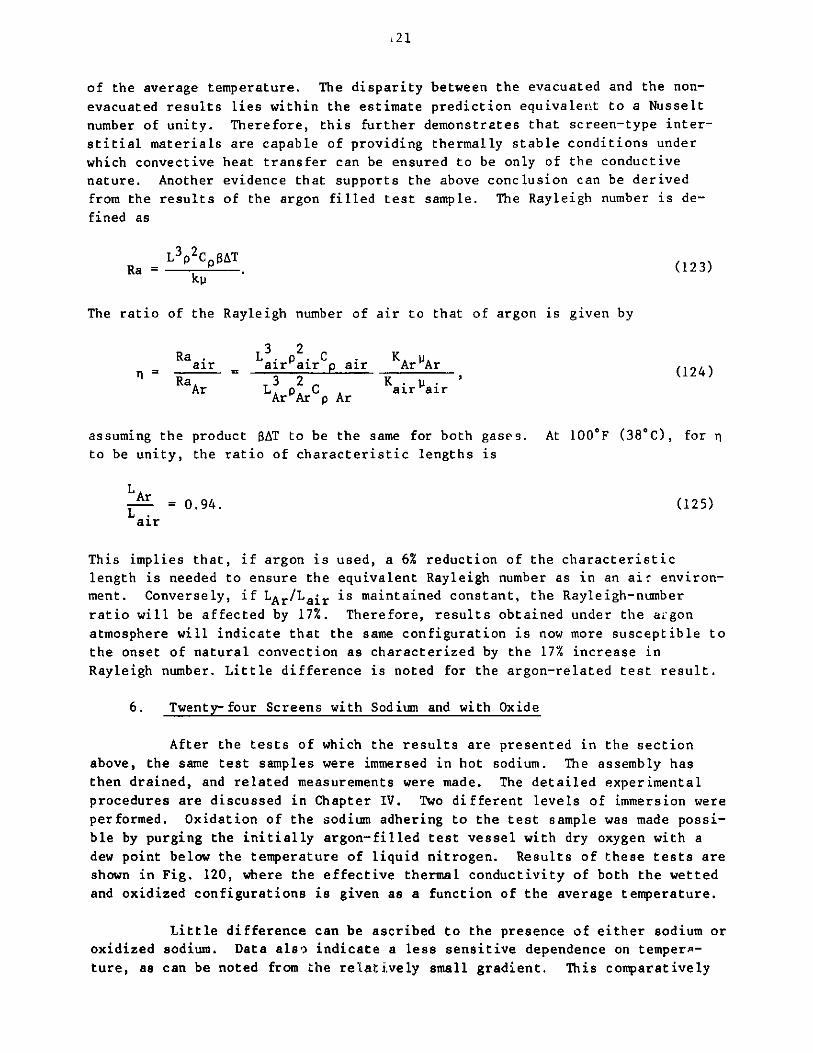
honeycomb core forming a sandwich-type thermal insulation, as shown in Fig. 14,
then, by arranging alternate layers of honeycomb core on face sheets, any
honeycombcore
face sha&tFig. 14
I
K4
Schematic Diagram ofHoneycomb Insulation)
\
29
thickness of such insulation could be made. This concept, on the other hand,
can be viewed as a multilayer reflective-shield insulation using honeycomb
cores as spacers. Also in the PLBR pool studies, other concepts such as the
"Solami" have also been explored by Collins (1978).
Most of the authors, in their study of heat transport through the insula-
tion, assume contributions from different modes of transfer, the sum of which
is the total amount of heat transferred across the insulation.
C. Contact Resistance
The study of contact resistance, also referred to as interface resistance,
can be dated back to the early forties when Mersman (1943) showed a one-
dimensional heat-conduction problem of two plane-boundary semi-infinite homo-
geneous solids of dissimilar materials with an imperfect contact along their
interface. This contact was t presented by a discontinuity in temperature at
the interface. After elaborate mathematical theorems were established, a complex
solution resulted. Schaaf (1974) later furthered such treatment by incorporating
a heat source in the original problem. Despite its practical applications,
interest in this area was primarily confined to exotic mathematical treatment due
to lack of adequate calculating facilities to render the subject more realistic.
This interest was revised in the sixties by the rapid development in the aero-
space industry. Precise understanding and knowledge of contact resistance is
critical in numerous space related heat-transfer studies, e.g., high- and low-
temperature shields (Barzelay, 1954, 1955). Aside from thermal radiation,conduction is the only other means of heat transfer in such environments.
Therefore, tip until the early sixties, thermal resistance was either esti-
mated or experimentally measured, e.g., by Willis and Ryder (1949) and Brunot
and Buckland (1949), or simply neglected.
Later some theoretical treatments analyzed heat transfer by conduction
through contacts and the interface fluid. Some used cylindrical geometries tomodel the contact areas. Contact surfaces of steel, brass, and aluminum were
also experimentally studied. Semiempirical analysis was made by using data on
steel to brass and steel to aluminum contacts. Fenech and Rohsenow (1963),
neglecting both radial-conduction and natural-convection heat transfer within
the contact area and using average boundary conditions, solved the Laplace
equation, from which they obtained an expression of thermal conductance across
the interface. Based on this approach, more detailed calculations using an
analog computer were reported by Henry and Fenech (1964). Clausing and Chao
(1965) summarized the assumptions inherent in theories presented up to 1965 in
the literature, in which (1) the actual areas of contact were uniformly dis-
tributed over the entire area, (2) the contact areas were circular, (3) the
asperities deform plastically under the load, so that the average pressure
exerted between them equaled the microhardness, and (4) the film surface resis-
tance was negligible. The authors further proposed a model where the contact
30
resistance was represented by the sum of the macroscopic constriction resis-
tance, microscopic construction resistance, and the film resistance of the
interface. Later, Clausing (1966) extended the model to describe heat transfer
between dissimilar metals. More refined theoretical treatments and experi-
mental data were presented by Clausing (1966), Mikic and Rohsenow (1966), and
Roca and Mikic (1971).
As the mathematical model describing the interface improved, the lack of
accurate information about the contact surface became more pronounced. Pre-
viously, different idealized models could assume certain well-behaved bound-
aries, whereas more sophisticated treatment required detailed data about the
contact surfaces. Clausing (1966) used the microscopic constriction concepts
to incorporate the surface into his model. Probabilistic density-distribution
functions were derived by Mikic and Rohsenow (1966) to account for variations
of the material surfaces. Different variances in different directions of the
surface were considered. Copper et al. (1969) further challenged the Gaussian-
distribution assumption of heights and proposed a different set of statistical
distribution functions arrived at considering the original surface profile.
More idealized treatment of the interface surface assuming parabolic con-
tacts was addressed by Yovanovich (1970), in which complex transformation to
the ellipsoidal coordinates provided a solution to the Laplace equation with
mixed boundary conditions. The thermal-contact resistance, it was reported,
was directly proportional to a geometrical function of the contact paraboloids.
Experimental results were also presented to substantiate the validity of the
theory. Effects of cyclic loading, over a pressure range of 4.45-34.5 x 10⁵ N/m2
(64.5-500 psi), on thermal conductance were measured experimentally by McKinzie
(1970). Agreement was found between data and theories proposed by Clausing
(1966) as well as McKinzie. Similar measurements were made by Cassidy and
Herman (1969) at ambient pressure of I atm (0.101 MPa) to 3 x 10-12 m/m Hg
(4 x 10⁻¹⁰ Pa), and limited agreement was calculated with Mikic theory. In
addition to accurately modeling the surface conditions, pressure distribution
on the interface was also considered in the theoretical treatment by Roca and
Mikic (1971)
Despite these exotic treatments on the subject of thermal-contact resis-
tance, there is still a chasm between engineering-application data and theories
developed, especially for complex geometrical contacts. experimental data for
soldered joints bolted or screwed sheet metal joints were reported by Yovanovich
and Tuarze (1969), and Veilleux and Mark (1969). Smuda and Gyorog (1969) con-
ducted an experimental investigation on thermal characteristics of materials
inserted between plane-parallel metal surfaces. Load pressures and mean junc-
tion temperatures were varied from 25 to 1000 psi (0.172 to 6.89 MPa) and -100
to 200 F (-73.3 to 93.3 C). Screens of various mesh sizes and materials were
reported tested where acceptable thermal-conductivity properties coupled with
their superb mechanical strength rendered the use of these materials as an
insulation uniquely attractive. Later, Gyorog (1970) further extended the
investigation to include other interstitial materials and configurations. Adimensionless correlation was presented, based on the functional relationships
of load, screen dimensions, and material properties. Notable improvements were
observed in thermal-insulation characteristics by separating the wire screens
with shim materials.
31
D. Convection
In 1900, Bernard experimentally studied the critical temperature gradient
that, when exceeded, would establish natural convection for horizontal plates
heated from below. Lord Rayleigh (1926) later laid the foundations for the
theoretical treatment of Bernard's experiment.
DeGraaf and Van Der Held (1952) later reported the observation of Bernard
cells by injecting smoke into the test cavity. The critical Rayleigh number
was found to be around 2000. Later, other studies were performed to further in-
vestigate the onset of natural convection between parallel plates. Chandrasekhar
(1971) summarized both the theoretical and experimental studies, where c criti-
cal Rayleigh number of 1709 was reported. Figure 15 depicts the Nusseit number
1.2 1-
300 500
1630
t_ ILI - -II Lt _t I I I L t I I I I I I V - I
1000 1500 2000 2500
Iti I I11! ff II 11 1 [ilia I I I III "I1I1I111 "771r--7n
I ,i S.0.
10
l" .'am 1 1 41 6 1 )0'd
-'fp
++
y
.. ,. 4 G 7S')1
' 2 .u 4 7
I ~I 1111 II11111 11111 II l~if 11111Cap111
I0U 10' 10+ 10' 10' 10' 10' 10'' 10
16a
Fig. 15. Nusselt Number vs Rayleigh Number for Parallel Plates. ANL Neg. No. 113-77-351.
w0
10
1.1
U.V'nt
lin
1-3r
32
as a function of the Rayleigh number. For Rayleigh numbers less than 1709, the
Nusselt number is virtually unity, implying that conduction prevails. It was
noted later that, by introducing side walls between horizontal plates heated
from below, thermal stability was further enhanced, thereby delaying the onset
of natural convection to a much higher Rayleigh number.
Theoretical treatments of infinitely long cylinders were presented by
Ostronmov (1958) and Yih (!959). Boundary conditions of perfectly condctingand perfectly insulating wall were both addressed. Analytically, Malku- and
Veronis (1958) used an integral technique, applied by Stuart (1958) to Lhemathematically analogous problem of predicting momentum transfer through a
fluid between two closely spaced, concentric rotating cylinders. Ostrach and
Pneulli (1963) had considered perfectly conducting walls of cylinders of arbi-
trary cross section using an approximation scheme. The results of Catton et al.
(1974) showed that the amount of suppression by continuing walls is a func-tion of both cavity-aspect ratios. Interferometric study of critical Rayleigh
numbers by Norden and Usmanov (1972) also helped to independently evaluate the
condition of natural-convection onset. Lighthill (1953) used the integralmethod to study natural convection in a closed-end tube of various aspect ra-
tios with constant-temperature walls. Experimental verification was obtained
by Martin (1955) and Harnett and Welsh (1957). Low Rayleigh-number convection
inside a spherical cavity was investigated by Drakhlin (1952). Using finite-
difference methods, Wilkes (1963) numerically solved the transient and steady-
state problems for natural convection in rectangular cavities with isothermal
walls and either perfectly conducting or perfectly insulating horizontal sur-
faces with a unity aspect ratio. It was demonstrated that, for a Rayleigh num-
ber of about 105, horizontal isotherms were observed in the interior with a
temperature gradient established in the vertical direction such that tempera-
ture increased upwards. De Vahl Davis (1968) concluded that, in a similar con-
figuration, the vertical temperature gradient in the center of the cavity is
essentially zero for small Rayleigh numbers. As for increasing Rayleigh num-bers, the slopes of the isotherms tend to become negative and the temperature
gradient approaches an asymptotic positive value, which is highly dependent
upon horizontal-wall conditions.
E. Radiation and Emissivity
The literature on beat transfer from radiating stationary media without
conduction, convection, and other energy-transfer mechanisms are summarized by
Jakob (1957). Early discussions by McAdams (1954) were confined to radiative
heat transfer in boiler furnaces and related areas. Radiative exchange between
surfaces separated by an absorbing and scattering medium involves considera-
tions of (1) the configuration of the surfaces, (2) the radiative properties of
the surfaces and the medium, and (3) their temperature distributions. In
McAdams (1954), Hottel used a finite-difference method to present a solution of
gray absorbing and emitting gas at constant temperature with heat source and
heat sink. An improved prediction was reported by Hottel and Cohen (1958),accounting also for variation of temperature in the medium. The solution to
33
the heat-exchange problem by radiation using the electrical-network method was
suggested by Oppenheim (1956). Bevans and Dunkle (1960) extended the concept
and solved a multinode network problem. A vigorous demonstration of the anal-
ogy of the electrical-network model to the solution of the two integral equa-tions that described the process of radiative heat transfer in a closed system
with absorbing and scattering surfaces was reported by Adrianov (1959), inwhich the two integral equations could be approximated by a system of linearalgebraic equations, which would result in the equivalent solution of the net-
work model.
Jakob (1957) has summarized the literature of configuration factors, alsoknown as views factors, shape factors, angle factors, or geometric factors, for
a few simple geometries for radiation through absorbing and nonabsorbing media.
Certain other straightforward geometries were investigated and tabulated by
Pittman and Bushman (1961), Hamilton and Morgan (1952), and Person and
Leuenberger (1957), and Tripp et al. (1962). Instead of evaluating the double-
area integrals, Sparrow (1965) proposed contour integrations whereby the ex-
pression was reduced to a simpler form. However, more complex but continuous
geometries will still have to be analyzed numerically. For highly discontin-
uous materials, approximations will have to suffice.
The term "radiosity" was defined by Hottel (McAdams, 1954) to denote the
amount of energy leaving a surface as a result of the energy emitted and re-flected by another surface. With this concept, n equations can be written for
an n-surface system based on the energy-conservation principle, whereby the
unknown variable can be solved. Gebhart (1961) introduced another method for
the solution of gray-body problems. Assumptions required by his method were
the same as those used for the Hottel method; that is, surfaces were gray,diffuse, and uniform in temperature.
Radiation-coupled conduction and convection can be divided into two cate-
gories. The first involves radiation passing through an absorbing emitting
medium, where net radiant energy is transferred to or from each element of themedium. Conduction and convection transfers can be treated as heat sources and
heat sinks, and the conservation-of-energy equation is an integrodifferential
equation. The other category deals with radiation interaction through theboundary conditions of conduction and convection processes. Viscanta (1960)
presented the first complete formulation of infinite parallel plates with an
absorbing medium, in which numerical iteration procedures were used to solve
the governing equation for several combinations of parameters. A thorough
treatment of radiation transfer coupled with free convection was presented byCess (1964), in which the ratio of the Nusselt number to the Grashof number wasexpressed in terms of an infinite series. Free convection without radiationreduces the expression to only the first term. Experimental investigations
were undertake n to augment the analytical studies, and reasonably good agree-ments were reported.
34
Emissivity is expressed as a ratio of a characteristic radiation emittedby a surface to that of a black body. There are different types of emissivi-
ties, depending on the various characteristics of the radiation; e.g., spectral
emissivity denotes the ratio of radiation of a certain wavelength emitted by
the surface conditions of the material to the emission of that wavelength from
a black surface. An oxide film of a few microns on the surface is sufficient
to alter its value significantly. Only literature pertinent to this study will
be reviewed.
Eckert et al. (1957) measured the total normal emissivity of porous mate-
rials by an energy balance between convective and radiative heat flow. Two
different types of porous surfaces were studied: Poroloy and modified Tyler
materials. The former was fabricated of Type 304 stainless steel wire wound on
a mandrel, layer after layer, to attain the desired porosity; then the material
was sintered. The latter was essentially composed of Type 304 stainless steel
screens fabricated by a special weaving process. High porosity and mesh sizes
showed increased total normal emissivity.
Wade (1959) and Wade and Slemp (1962) reported that oxide coating forma-
tions were observed on all their Type 347 stainless steel samples at an oxida-
tion temperature of 2000 F, and total normal emissivity values changed from 0.3
to 0.85 in the order of hours. A comprehensive literature survey was summa-
rized by Touloukian (1970) in which emissivities of different types of stain-
less steel under different conditions were presented. The effects of surface
films on radiative properties of metallic surfaces was treated theoretically by
Cravalho et al. (1969), in which the relative effect was found to depend on the
reflective index of the film, and naturally occurring oxide films had no effect
on the total hemispheric-radiation properties except at high temperatures.
Brannon and Goldstein (1969) reported that an increase in oxide-film-layer
thickness would result in a similar increase of emissivity.
Information on emissivity values of sodium oxide is extremely limited and
incomplete. To my knowledge, there is no good documentation on such measure-
ment for sodium oxide. Through private communication with the staff of Atomics
International, I determined that some crude experimental measurements were made
on sodium oxide on one occasion in which the emissivity value was estimated to
be between 0.9 and 1.0.
F. Gas Conduction
When the value of the Rayleigh number is well below the threshold at which
natural convection occurs, conduction prevails. This becomes especially
straightforward for gaseous conduction between parallel plates. On the other
hand, gas conduction within honeycomb configurations lately has also received a
great deal of attention, primarily from the standpoint of solar-energy applica-
tions. Studies include thermal stability and heat transfer of inclined honey-
comb cells, e.g., reports by Randall et al. (1977) and Buchberg et al. (1976).
Attention is focused primarily in trying to minimize convection in order to
35
prevent heat losses. Various aspect ratios have been investigated, and rectan-
gular cell structure is found to be an effective device to suppress natural
convection. Under this condition, the application of the heat-conduction equa-
tion to account for the gas-conduction heat transfer is sufficient. Thermal
stability for irregular cell sizes and geometries has not received much at-
tention. Since the convection onset depends heavily on the cell geometry,
arbitrary configurations limit the ability to pursue any meaningful studies.
However, given the configuration presented by layers of screens stacked to-
gether, thermal-stability analysis of other fundamental geometries--namely,
horizontal cylinders, vertical flat plates, and inclined flat plates--will have
to suftice as some form of estimate of the complex geometry.
Another kind of gas conduction has not been addressed previously, namely,
heat transfer in rarefied gases. Despite the fact that, in reactor applica-
tions, this type of energy transport is extremely uncommon, experiments were
selected for this study to test all insulation assemblies under evacuated
conditions in order to be able to better distinguish various forms of heat
transfer. If the mean free path of gas molecules is large compared to the
characteristic system length, conduction can be approximated well by Knudson's
formula. However, given the equipment-design criteria, the contribution from
rarefied-gas heat transfer is not measurable by the existing setup. Therefore
it will be assumed that, for low-density gases, conduction can be neglected.
C. Sodium and Sodium Oxides
One consequence of using liquid sodium as a heat-transfer fluid is the
formation of sodium aerosols during high-temperature operation that can be
transported to and deposited on different components, causing unnecessary main-
tenance. Since requirements of high thermal efficiency prevail, the operating
temperature of the primary sodium is about 1000 F (538C), and the amount of
sodium aerosols generated increases proportionally with temperature. This is
clearly shown in Fig. 10, where the vapor pressure of sodium is plotted against
temperature. An increase of 100 F, from 900 to 1000 F (482 to 538C), in tem-
perature will result in a fourfold increase in vapor pressure. Therefore, to
estimate the amount of aerosols produced, the rate of vapor-nuclei formation
can be evaluated, and or:: method is suggested by Sheth (1975). Vapor agglomer-
ation will occur when aerosols of various sizes are formed. Knowledge of ag-
glomeration dynamics implies an ability to calculate aerosol sizes that are
critical in removal mechanisms or other sodium-related investigations, as de-
scribed by Files et al. (1976). The authors provide a comprehensive treatment
of aerosol removal by settling, surface plating, leakage, and ventilation.
Nonetheless, forces that affect aerosol transport behavior are equally impor-
tant to be understood. Brownian motion arises from the collision of ae osol
particles with cover-gas molecules in thermal motion.
Gravity is another type of force to which aerosol particles are subjected.
Both of these forces are dealt with by Greenfield et al. (1969). Force and
36
free convective forces are addressed also by Castelman et al. (1969). Other
resis (mass concentration related), and photophoresis (light related) can also
influence aerosol behavior; however, because of their limited influence in this
study, they are not considered here.
To a greater or lesser degree, the operating experience of an LMFBR re-
lates to the difficulty imparted from sodium aerosols and vapors in the cover
gas. EBR-II reported sodium buildup from aerosol transport on the seals of
rotating plugs, as discussed by Cooper (1969). Similar problems were also
encountered at the Fermi Reactor. During the 10 years of operation at RAPSODIE
and 3 years at PHENIX, problems of condensation of sodium in annular spaces
were encountered. Plugging also occurred in gas pipes, filters, and vapor
traps. The KNK Reactor reported that nonhomogeneously distributed deposits
were formed between the large utility plug and the reactor vessel. These oc-
currences can be attributed to the geometry of the components and their maldis-
tribution of temperature. Joyo also received its fair share of aerosol-related
difficulties, and before Monju was built, a vigorous research and development
program was launched to overcome such problems. These are some of the examples
reported by the International Working Group on Fast Reactors [Himeno (1976)]
et al. to illustrate the immense task of circumvention of sodium-aerosol trans-
port. All countries who participate in LMFBR developments are engaging in
experimental and/or analytical programs intended to reduce and control sodium-
aerosol transport, as described by the International Working Group on Fast
Reactors, IAEA (1977). Other sodium-related experiences are summarized by Funk
(1974).
Of all the aforementioned means by which sodium aerosols are transported,
convection is the most important. Diffusion or Brownian movement only becomes
significant when the transport time due to convection is on the order of the
diffusion time. Under typical reactor operating conditions, convection will
prevail. The impacts of both natural and forced convection depend on a number
of parameters: temperature gradient, temperature, geometrical configuration,
fluid properties, and the velocity of the flow. For simple geometries and
idealized conditions, both types of convection have received much attention,
some of which, for natural convection, is given in Sec. II.D above. In EBR-II,
forced convection has been introduced properly around annular regions, e.g.,
various types of components seals, to eliminate natural-convection cells formed
from temperature maldistribution. Since both types of convection are highly
sensitive to geometrical configurations, a thorough and complete analytical or
experimental effort to model the deck structure and the cover-gas space is not
entirely realistic. Simplified models by Shimazaki (1970), (1975) attempt to
predict deposition rate and distribution of sodium aerosol due to th ermal
convection.
In a separate effort, evaporation from a sodium-pool surface was studied
experimentally and, in parallel, a mathematical model of vapor formation was
developed by Himeno et al. in JAPFNR-243 (1976). Deposition in an annulus
37
within an enclosed cover-gas space is also addressed by Himeno et al. in
JAPFNR-245 (1976). Results of distribution within an annulus versus distance
from the inlet are given. Similar studies are being made in the United Kingdom
and the United States.
The conversion of sodium to different types of oxides (namely, sodium
oxide, Na20, and sodium super oxide, Na2 2) due to the presence of oxygen from
the cover-gas system, regular maintenance leakage, and residual oxygen of the
structure and components, further complicate the situation. Oxides of sodium,
unlike sodium metal, exhibit characteristics such as low thermal. conductivity,
high emissivity, low ductility, and high melting temperature. This markedly
different behavior in physical and chemical properties of sodium oxides make
controlling vapor transport difficult. Elevated temperature was used in the
German RSB facility to change the condensed sodium deposit into its liquid
state, i.e., rwre sodium metals, whereby it can be drained back into the sodium
pool. However, if a substantial amount of sodium oxide is present, the viscos-
ity of sodium and sodium oxide mixture, coupled with poor wetting, may prevent
effective drainage, as discussed by Jansing et al. (1977).
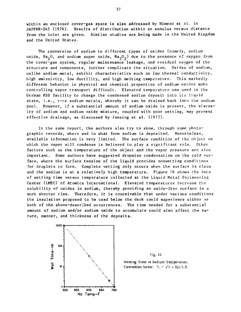
In the same report, the authors also try to show, through some photo-
graphic records, where and in what form sodium is deposited. Nonetheless,
available information is very limited. The surface condition of the object on
which the vapor will condense is believed to play a significant role. Other
factors such as the temperature of the object and the vapor pressure are also
important. Some authors have suggested dropwise condensation on the cold sur-
face, where the surface tension of the liquid provides nonwetting conditions
for droplets to form. Complete wetting only occurs when the surface is cleanand the sodium is at a relatively high temperature. Figure 16 shows the data
of wetting time versus temperature collected at the Liquid Metal Engineering
Center (LMEC) of Atomics International. Elevated temperatures increase the
solubility of oxides in sodium, thereby providing an oxide-free surface in a
much shorter time. Therefore, it is conceivable that under various conditions
the insulation proposed to be used below the deck could experience either or
both of the above-described occurrences. The time needed for a substantial.
amount of sodium and/or sodium oxide to accumulate could also affect the na-
ture, manner, and thickness of the deposits.
1000
100
E o Fig. 16
Wetting Time vs Sodium Temperature.3 10 Conversion factor: C =_(*F - 32)/1.9.
500 550 600 650 700
Na Temp-F
38
III. ANALYTICAL STUDIES
A. Thermal Convection
1. Natural Convection
A few geometries are of particular interest in convection heat trans-
fer as they pertain to the different types of thermal insulation. They can be
identified as the spaces between horizontal parallel plates, the square cells
of the honeycombs, and the interstitial spaces between layers of screens.
Closely coupled with the question of geometry is the determination of the con-
ditions of the onset of thermal instability, which will result in convection
heat transfer.
Based on the basic hydrodynamic equations, namely, the continuity,
linear momentum and energy, and by using the Boussinesq approximation, which
assumes that p is a constant in all terms except the external-force term,
Chandrasekhar (1971) obtained the analytical solution for an infinite horizontal
layer of fluid in which a steady temperature gradient is maintained. Three dif-
ferent types of boundary conditions were examined: the free surfaces where
there is no tangential stresses, tne rigid surfaces where no slip occurs at the
boundaries, and the combination of these conditions.
For the free surfaces, the Rayleigh number is about 657; for both
rigid surfaces, the Rayleigh number is 1708; and for the combined situation,
the Rayleigh number is 1100. Experimental efforts by Schmidt and Milverton
(1935), Silveston (1958), and others confirmed the analytical results that
there is only heat transfer by the conductive mode for Rayleigh numbers below
the critical value, e.g., ~1700, in Fig. 15.
Between the Rayleigh number values of 1700 and 3200, the increase in the
value of the Nusselt number follows a nearly linear relation. The flow pat-
terns were first observed by Bernard (1900), who reported the formation of
cells of similar sizes within which convection prevails, as shown in Fig. 17.
Suppression of the existence of these convection cells will result in a unit
Nusselt number, characterizing conduction heat transfer. Therefore, this can
be simply applied to calculate conduction and convection heat transfer between
horizontal plates. In Fig. 18, the Rayleigh number,
2 3p 2gATC L
Ra= pk(1)ku '
where
p = density,
= coefficient of expansion,
AT = temperature difference,
39
L = characteristic length,
k = thermal conductivity,
u = viscosity,
and
Cp = specific heat,
is plotted as a function of AL 3 for three
helium. Air has never been and never will
but it is presented for the convenience of
extraordinary ability of helium to maintain
the figure.
different fluids: air, argon, and
be considered as an LMFBR cover gas,
later experimental analysis. The
thermal stability is evident from
2500
-9 --- -
I I I I I ,/-ot ~ o
2000
1500
1000 -
500 -
0-HEATED
Fig. 17. Flow Pattern for Bernard Cell0
Temp 1500
Ar
1AirI1
Ra= 17601HI,
1111
11
i111
1f
He
0.4 0.8 1.2
T L
Fig. 18. Rayleigh Number vs ATI3 for Paral-lel Plates. Conversion factor: C =
( F - 32)/1.8.
Different authors have demonstrated that the presence of lateralwalls reduces or even suppresses natural convection between horizontal surfaceswith the lower surface maintained at a higher temperature. The Malkus power-integral technique can be adopted to estimate the amount of heat transfer frombelow within such an enclosure, as described by Edwards (1969). It uses anintegral expression derived from the energy-conservation equation. The approx-
imate velocity and temperature profiles of the most unstable convection, whichare derived from a linear perturbation analysis of the equations of motion, aresubstituted into the expansion to obtain the final solution. Two differenttypes of sidewall boundary conditions can be assumed: a linear wall temperature
11.6 2
,......
i
40
in the upward direction, and an adiabatic condition between the fluid and the
wall. At any vertical position, the vertical heat flux consists of a conduc-
tive and a convective term
q=-Kk T+ pC VT, (2)az p z
where Vz is the vertical component velocity.
The total upward heat transfer per cell is therefore the sum of
vertical heat flux of the fluid and of the wall:
Q = Aw K<-aT/z> + A fKf<-aT/az> + AfpC (Vz T>,
where the brackets denote a vertical average and the bar denotes a horizontal
average. It is further assumed that only horizontally symmetric temperature
profiles are considered. This implies that, for the most unstable disturbances,
the net heat transfer between the fluid element and the wall element vanishes.
If L is the height of the cell and -(a/az)T is written as (Th - Tc)/L, where
Th and Tc are the hot an, cold temperatures, respectively,
- ( V T>Nu = L __ _ 1 + -zL
K Th - Tc a<-T/z> K Th - Tc(4)
The Nusselt number is known only if the temperature and velocity profiles are
known. If the velocity vanishes, representing a special case in which only
conduction prevails, the Nusselt number reduces to unity, as expected. Sub-
stitution of the velocity and temperature profiles obtained from perturbation
study would enable the evaluation of the onset of natural convection within
such cells.
The temperature profile can be written as the sum of an average
temperature and a small temperature perturbation:
T(x,y,z) = T(z) + T'(x,y,z). (5)
When Eq. 5 is coupled with the continuity equation that specifies
fdx dy VV~ =f z = 0, (6)z fdxdy
it follows that
VzT VzT.(7)
Similarly to Eq. 5, the velocity distribution can be written as
V (x,y,z) - -V' -f. . . (x,y) g (z) (8)z z i.9J.9 ,t ,3 zk
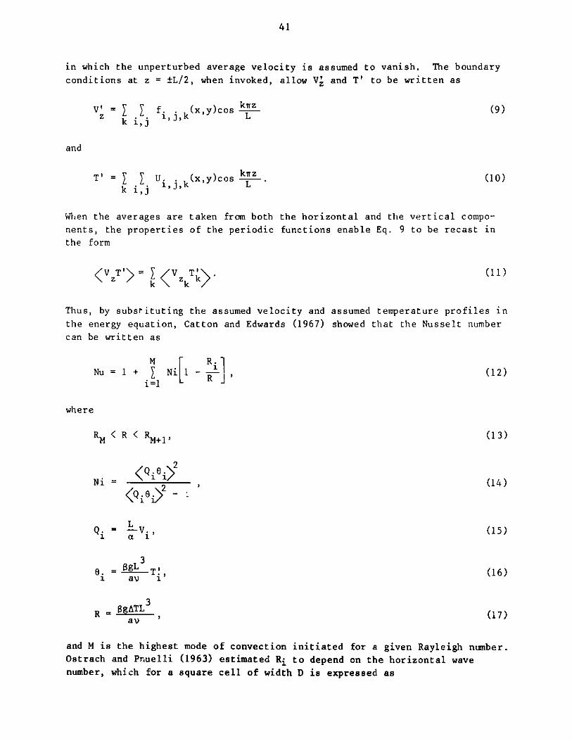
41
in which the unperturbed average velocity is assumed to vanish. The boundary
conditions at z = L/2, when invoked, allow V, and T' to be written as
V' =G f. . (x y)cos kiz (9)k i,j
and
T'= U. . (xy)cos krz .(10)k i,j ij,k L
When the averages are taken from both the horizontal and the vertical compo-
nents, the properties of the periodic functions enable Eq. 9 to be recast in
the form
<VzT'> = zkT >. (11)
Thus, by substituting the assumed velocity and assumed temperature profiles in
the energy equation, Catton and Edwards (1967) showed that the Nusselt number
can be written as
M R.Nu = 1 + NiL1 - R J , (12)
i=1
where
RM < R M+1, (13)
.<i
Ni = (14)
Qi= L (15)
_ L
30. = gL (T,(16)i av 1
R = SgATL3
av
and M is the highest mode of convection initiated for a given Rayleigh number.
Ostrach and Pnuelli (1963) estimated Ri to depend on the horizontal wavenumber, which for a square cell of width D is expressed as
42
nLF5a = D (18)
If the walls of the cell are perfectly conducting, the horizontal wave numberwill be the same as shown by Eq. 18. For adiabatic walls, the adjusted wavenumber is
a' = 0.75 L/7D for conducting walls (19)
and
a' = a for diabatic walls. (20)
The vertical and horizontal wave numbers for closed cells can be approximated
by
bi = kiT + 0.85, (21)
2 biA. = a + -- , (22)1 2'
and
(Ai + b'23R. = . (23)
A.1
The values of Ni for infinite horizontal surfaces were determined by
Catton et al. (1974) and are presented in Fig. 19 and Table II. These valueswill be used as an approximation for Ni. A limited application of the abovemethod was reported by Sun and Edwards (1970), where rectangular cells ofratios 2 and 3.6, and 4 and 15.2 were examined for aspect ratios of 4 and 3.87,respectively. For reference, experimental data were also presented for stain-less steel, as plotted in Fig. 20. The data collected only for stainless
=9 i=72.0======-
...-.- -=
2u .5- Fig. 19
Ni vs wave Number a
1.011 1-- -0 10 20 30 40 50 60
Wove Number a
43
TABLE II. Values of Ni as a Function offrom Catton (1966)
Wave Number a,
Values of i
a 1 3 5 7 9
1.0 1.435 1.745 1.850 1.918 1.974
12.0 1.609 1.777 1.865 1.927 1.981
21.0 1.737 1.813 1.881 1.937 1.990
30.0 1.806 1.847 1.898 1.948 2.000
42.0 1.857 1.882 1.921 1.965 2.000
54.0 1.888 1.907 1.940 1.980 2.000
.-
-JU,N,D
6.05.0
4.0
3.02.5
2.0
I .5
Sun and Edwards (1970)
O CELL I L/d=1.54 H=1.26o CELL 2 L/d=I.00 H=2.16 ',6
-- THEORY ITHEORYa
2x1C) 4 4x10⁴ 6x10⁴ I 0 2Kx05RAYLEIGH NUMBER BASED ON HEIGHT
6x10³ 104 4 x10⁵
Fig. 20. Nusselt Number vs Rayleigh hum-ber for Stainless Steel Cylinder
steel cylinders, show that, with L/D equal to unity, the critical Rayleighnumber is about 2 x 10⁴ , which is considerably higher than for parallel plates.
2. Natural Convection within a Porous Medium
The phenomenon of natural convection through porous media hasreceived increasing attention due to its widespread applications, principallyin the areas of geophysics and thermal-insulation designs. Under the assump-tion that the space to be considered is homogeneous, th2 actual flow of fluidin a porous medium from a phenomenological standpoint closely resembles thehypothetical convective motion in a fluid layer of the same rate. However,the flow-resistance expressions for the two cases do differ in that, for porous
1 I 1 . 1i n L.%..
44
media, instead of the shearing stress being proportional to the velocity
gradient, Darcy's Law is applied,
(flv = -Vp, (24)
where p is the viscosity, K is the permeability of the medium, V is the
macroscopic velocity, and p is the pessure of the fluid. If Cartesian
coordinates are adopted for the porou3 medium that is uniform between two
horizontal impermeable surfaces separated by a distance 2, the equations of
continuity, motion, and energy can be expressed as
Dp+ pV = f + V.- (pV) = 0, (25)
p = N ~+ pV . VV = -pg -Vp- -- V, (26)D t 3t N~ ^~ ~ K ~
and
DT = a 2 T, (27)
where p is the density of the fluid, g is the vector presentation of gravitation
acceleration, T is the temperature of the porous medium, and a is its thermal
diffusivity. Note that the conventional viscosity term is replaced by Darcy's
Law, which is valid for Reynolds number based on one pore diameter being less
than unity, as stated by Lapwood (1948).
Based on these Pquations, the onset criterion of natural convection
can be evaluated for the "z components in ways similar to those used to pre-
dict the horizontal fluid layer, except for vanishing velocity boundary condi-
tions at z = 0, X. Lapwood derived the condition to be
Ra K = 4r2 (28)
where
3Ra = SC RAT (29)
va
in which S and v denote, respectively, the coefficient of expansion and the
kinematic viscosity, and AT represents the temperature difference between the
bounding surfaces. Before Eq. 28 can be used, two parameters would first have
to be determined: the medium's thermal diffusivity and its permeability K.
Strictly speaking, the time-dependent density derivative in Eq. 25
should be replaced by (3/3t)ep, where e is the porosity of the medium. How-
ever, in obtaining Eq. 29, we assume the variation of density to be negligible
except due to temperature differences. Second-order approximation terms are
neglected. Lastly, it is also assumed that the criterion of onset rendered
the partial time derivative zero.
45
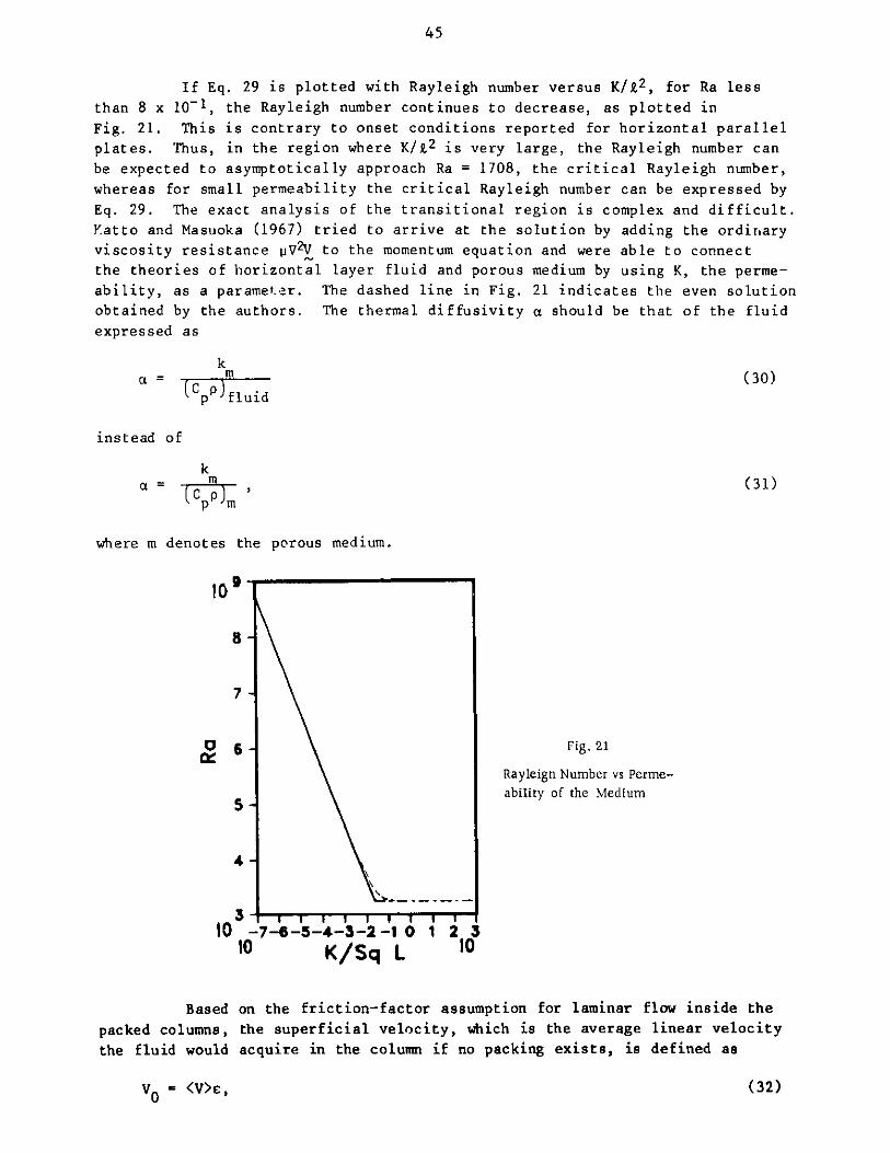
If Eq. 29 is plotted with Rayleigh number versus K/l. 2, for Ra less
than 8 x 10⁻¹, the Rayleigh number continues to decrease, as plotted in
Fig. 21. This is contrary to onset conditions reported for horizontal parallel
plates. Thus, in the region where K/R 2 is very large, the Rayleigh number can
be expected to asymptotically approach Ra = 1708, the critical Rayleigh number,
whereas for small permeability the critical Rayleigh number can be expressed by
Eq. 29. The exact analysis of the transitional region is complex and difficult.
Katto and Masuoka (1967) tried to arrive at the solution by adding the ordinary
viscosity resistance pi 2V to the momentum equation and were able to connect
the theories of horizontal layer fluid and porous medium by using K, the perme-
ability, as a parameter. The dashed line in Fig. 21 indicates the even solution
obtained by the authors. The thermal diffusivity a should be that of the fluid
expressed as
ka = m (30)
aCpfluid
instead of
ka = m (31)
p m
where m denotes the porous medium.
10'
8
7
0 6 .Fig. 21
Rayleign Number vs Perme-
5 -ability of the Medium
4
3-1'10 -7-6-5-4-3-2-1 0 1 2 3
10 K/Sq L 10
Based on the friction-factor assumption for laminar flow inside the
packed columns, the superficial velocity, which is the average linear velocity
the fluid would acquire in the column if no packing exists, is defined as
V0 (3>E,2(32)
46
where e is the void fraction
_ Volume of voidVolume of bed
Based on the Fanning friction-factor expression, the average velocitycan be written as
(P. - PQ)R21 O K
<V>= 2 L(34)
where R, is the hydraulic radius,
R = Cross section available for flow (35)K Wetted perimeter
and can be further written as
Volume of void
R = Volume of bed _C (36)K Wetted surface
Volume of bed
Using Eq. 36, we can rewrite Eq. 32 as
P - P 2V _ 0 L E . (37)0 2jjL 2
With the application of Darcy's Law (Eq. 24), the permeability of the medium,
K, can be expressed as
3K = . (38)
22
47
B. Thermal Radiation
Thermal radiation is recognized as energy in the form of electromagneticwaves with wavelength, in general, ranging from 3 to 13 pm emitted by a medium
due solely to the temperature of that medium. The Stefan-Boltzmann equationdescribes the energy flux for black body radiation,
Eb T) = n2 aT4 , (39)
where n is the index of refraction and a is the Stefan-Boltzmann constant.
However, normally encountered media and surfaces do not generally satisfy this
equation. Consequently, assumptions and modifications of the equation will
have to be made to better describe real media and surfaces. The assumptions
are summarized as follows.
1. Gray body: This implies that ea and ax are both independent of wave-length. In reality, very few matrials satisfy this assumption over the entire
range of wavelengths. Nevertheless, for finite range considerations, this will
suffice as a good approximation.
2. Diffuse: This denotes directional uniformity. In other words, the
intensity of the radiation leaving a surface resulting from emission or reflec-
tion is uniform in all angular directions.
3. Local thermodynamic and radiation equilibrium: This assumption al-
lows the existence of a nonisothermal system in which the temperature within
the system will be defined unambiguously. Radiation equilibrium requires the
amount of radiant energy absorbed per unit time by a given volume to be equalto the amount of radiant energy emitted per unit time by the same volume.
According to Kirchhoff's Law, in a particular direction and for each component
of polarization, the monochromatic emittance eX and the monochromatic absorp-tance as are equal. That is,
E
eE() = = a(8i). (40)ab
As a consequence of the above assumptions, the following equality resulted:
ex - aX. (41)
With the introduction of these assumptions, radiative heat transfer between
surfaces can be described sufficiently accurately without requiring a knowledge
of quantum mechanics and electromagnetic theory. Different theories using the
above assumptions are discussed briefly below.
48
Az, dA2
r
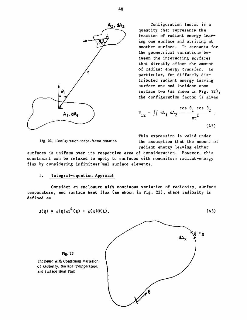
Configuration factor is aquantity that represents thefraction of radiant energy leav-ing one surface and arriving at
another surface. It accounts forthe geometrical variations be-tween the interacting surfacesthat directly affect the amountof radiant-energy transfer. Inparticular, for diffusely dis-tributed radiant energy leavingsurface one and incident uponsurface two (as shown in Fig. 22),the configuration factor is given
cos 6 cos 0
F1 2 = ff d 12 2nr
(42)
This expression is valid underFig. 22. Configuration-shape-factor Notation the assumption that the amount of
radiant energy leaving either
surfaces is uniform over its respective area of consideration. However, this
constraint can be relaxed to apply to surfaces with nonuniform radiant-energy
flux by considering infinitestImal surface elements.
1. Integral-equation Approach
Consider an enclosure with continous variation of radiosity, surface
temperature, and surface heat flux (as shown in Fig. 23), where radiosity is
defined as
J() - c( )dr4() +p( )G()
Fig. 23
Enclosure with Continuous Variationof Radiosity, Surface Temperature,and Surface Heat Flux
dAC
(43)
49
where G(T,) denotes the incident radiant heat flux upon position E, and n is
assumed to be unity. The local heat-transfer rate at X in the enclosure is the
difference between the emitted radiant flux and the amount of incident
radiation absorbed. That is,
q(X) = E(X)aT4 (X) - a(X)G(X). (44)
With Eq. 43, the radiosity can be reexpressed as
J( ) = e(E)aT4 () - 2i[q(E) - E(E)cT4 ()]. (45)
If the enclosure is opaque, then,
E(U) + p( ) = 1 (46)
and
4 1 - eU)J(&) = aT () - e)q(-).-(47)
Since all the radiation incident upon an element of an enclosure comes from
other elements that make up the enclosure, the incident radiation heat flux can
be written as
G(x) = f J(E)dFdx-dC. (48)
When Eq. 43 is recast into a different form, the radiosity at x becomes
J(x) = E(x)aT4 (x) + 1 - e(x) J J(E)dFdx-dE (49)
and combining Eqs. 47 and 49, we obtain
= aT 4 (x) - f dT()dFdx-d + [1 - E(C)] dFdx-d&. (50)
If the temperature is prescribed, the heat-flux distribution can be
calculated from Eq. 50. Conversely, if the heat flux is provided, the tempera-
ture distribution can be determined. This represents two different heat-
transfer processes in which the gray-body energy exchange is characterized bythe first two terms of the right side of the equation. The last term denotesthe energy exchange resulting from geometrical reflections of different ele-ments within the enclosure.
2. Finite-difference Approximation
The integral equation given in Eq. 50 is generally difficult to
solve, sometimes even for simple geometries. For this reason a finite-difference approximation is formulated. Instead of examining infinitestimal
50
elements, we choose a finite number of small subareas such that the radiosity
over each subarea is assumed to be constant. The radiosity for subarea i is
therefore
4J. = E.aT. + p.G.. (51)
1 1 1 1 1
From the energy balance between subareas within an enclosure, the total amount
of radiant energy arriving at subarea i is
NG. = I J.F. ., (52)
j=1 1J
where N is the number of subareas within the enclosure. The local heat-
transfer rate at subarea i is given by
4q. = e.aT. - ac.G.. (53)
1 1 11
Combining Eqs. 51 and 52, we obtain
J. = e.aT. + i (q. - E.aT.). (54)1 1 1 a. 1 11
If the enclosure is opaque, implying that the sum of the emittance andreflectance is unity, then,
E. + p. = 1 (55)1 1
and
4 - 1 56J.=4T l q.. (61 ..1
Using Eq. 52, we can further eliminate the radiosity to obtain
The first term clearly shows the gray-body energy exchange; the second term
describes the geometrical reflection between surfaces. Equation 58, in es-
sence, is the finite-difference representation of Eq. 50, for which a numerical
solution can be obtained, provided that a sufficiently large number of mesh
points are used. Various similar approximation methods, namely, Hottel'smethod, Gebhart 's method, and the Network method, can all be derived from these
finice-difference approximation equations.
3. Network Method
It is recalled from the definitions of radiosity (Eq. 51) and localheat-transfer rate (Eq. 53) that, if the incident radiant heat flux is elimi-
nated from these equations, the result is
R- I-EAF12 EA
I
--E I
~ I
-P I-E3A2F AF
I -
A 2¬ 2 AF12 A1¬ 1
Fig. 24. Equivalent Networks f
Energy Exchange betwe
Surfaces
q. = J. - G.,1 1 1
- 1 (aT'; -(a) (59)
where analogy can be drawn between the above equa-
tion and the Ohm's Law expression. The quantities
(1 -ei)/ei, qi, and (aT - Ji) can be interpreted
(b) as the "resistance" to radiant heat flow, the
"current" of heat transfer, and the "potential
difference" between two imaginary surfaces,
respectively. Equation 59 and its electronic-
circuit equivalent are depicted in Fig. 24a. When
the emittance Ei approaches zero, regardless of
(c) the surface temperature, there is no heat transfer
away from surface i. As ci becomes unity, thethermal resistance, (1 - Ei)/ci, vanishes andconsequently, Eq. 59 reduces to the simple fact
(d) that the radiosity is the black-body emissive
power.
or Using Eq. 52 and the local heat exchangeen between surface i and its surroundings given by
the difference between radiosity and irradiation,
(60)
we can write the heat-transfer rate as a function of radiosities from different
surfaces and their respective configuration factors.
52
n nq.= J. - J.F. = (J.- J.)F... (61)
i1 1 3 J 1 3 =1 1 3 3
n
The identity F.. = 1j=1 '1
has been used to arrive at Eq. 61. If the radiosities Ji and Jj are inter-
preted as thermal potential nodes, Eq. 61 becomes a summation of these thermal
potential differences between surfaces within the enclosure where the resis-
tance between nodes is dependent upon the surface areas and their respective
configuration factors. This is also illustrated in Fig. 24b.
Authors such as Sparrow (1965) and Kreith (1976) extended this con-
cept and arrived at a network model of radiant energy exchange as depicted in
Fig. 24a in which each black-body emitter is denoted by a battery acting as adriving force. The black bodies are typically connected together through two
resistors, each representing the gray-body approximation and the geometrical
resistance in energy transfer. This electric-network analogy allows the appli-
cation of linear rules of electrical circuit, namely, Kirchhoff's Law, to many
body-energy exchanges in which simplicity and linearity of the equations are
preserved.
This basic approach is commonly used by others in formulating their
solutions, such as Tien and Cunnington (1969), Fletcher (1970). However, note
that the network model given in Fig. 24 is not the result of direct derivation
from fundamental equations. The two equations that form the basis of the net-
work model and are dedIuced from first principles are Eqs. 59 and 61. Each of
them describes precisely only the energy-exchange relationship between itself
and its immediate surroundings, as depicted in Fig. 24. When the system in-
cludes only two surfaces, attempts in connecting the two surfaces results in a
network shown in Fig. 24d.
Further efforts in connecting multiple surfaces together, e.g.,
Fig. 24c, exemplified an inherent assumption. Energy transfer from one black
surface to another follows the most direct path, i.e., the connection along
which there are the least number of resistors. Since, for the two-surface
system, the shortest path between the surfaces happens to be also the only
path, the above assumption seems to be superfluous. But as one examines a
three-body system (Fig. 24c), energy leaving surface 1 traverses to surfaces 2
and 3 via path 12 and 13, and if the three surfaces are assumed to be of a
black-body nature, radiant energy arriving at surface 3 by path 23 is totally
independent of surface 1. This implies that, once radiant energy impinges upon
any of these surfaces, its earlier history of where the energy originates be-
comes irrelevant to any subsequent energy-transfer calculation. The energy
exchange between surfaces 1 and 2 is
(62)q12 - A1F12(Ebl - Eb2),9
53
where 1/A1 F12 is the thermal resistance. This differs from results obtained by
evaluating the effective thermal resistance of the three resistors based on the
theory of electric circuits, namely,
1 = 1 1 + A1F 1 2 . (63)
A2F23 AF13
For a two-body gray-surface system, the network representation that
is a direct reduction from the basic equations accurately models the energy
exchange between the surfaces. However, similar network representation for
three-body interaction poses a few difficulties if caution is not exercised in
reducing solution from the model. Figure 24c illustrates the fact that energy
exchanges between each pair of radiosity nodes, viz., J1 and J2, J 3 and J2 , and
J1 and J3 , satisfy the equation
r12 R 1 2), (64)12
where q12 is the energy exchange between the radiosity nodes J 1and J2 and F12is the configuration-factor resistance between those two surfaces. But in
order to ascertain the net heat-transfer rate from surface 1 to surface 2, the
network-resistance equivalent between the two points of interest yields
with Fij i,j = 1, 2, 3, denoting the configuration-factor resistance betweensurfaces i and j. The network equivalent model further predicts that theradiant-energy exchange between surfaces 1 and 2 is inversely proportional to
the effective thermal resistance (Eq. 64) multiplied by the difference in ther-mal potential, given by the black emissive power between the said surfaces.
That is,
q = -(Ebl - Eb2). (66)
As the emittance of surface 3, e3, approaches zero, implying that it
is a perfect reflector (p3 = 1), there is a maximum amount of energy transfer
between surfaces 1 and 2. Conversely, when surface 3 is a black body, energy
transfer is minimum. Careful examination of Eq. 64 shows that the effectivethermal resistance is only dependent upon the configuration factors, emittance,and areas of respective surfaces. Consequently, changes in the radiative prop-
erties of surface 3 have little effect on the overall energy exchange betweenthe other two surfaces. Similar difficulty also occurs when the model is ex-
tended to many-body exchanges.
54
4. Gebhart Method
The basic assumptions of this method entails the gray-bodyapproxi i -of interaction and diffuse surfaces. Gebhart, who introduced
this method, denoted the fraction of
radiant energy absorbed by surface jto that which is emitted by surface i
as Gj1 . This fraction of radiant
A Fienergy includes the direct'radiantA. energy transfer and any other transfer
through multiple reflections within
the enclosure from surfaces i to j.
For an enclosure with n surface ele-
ments as depicted in Fig. 25, the
F.n energy balance between surface i and
surface j can be summarized as
n
G.. =E.F.. + pkF. G,13 J IJ k=1k kj
(67)
An where Fij denotes the fraction of the
amount of total direct energy emitted
Fig. 25. Enclosure to Illustrate the Gebhart Method by surface element i that is absorbed
by element j and is the definition of
configuration factor. The summation represents the exchanges through reflec-
tions. For example, when k = 1, the term p1 Fi1 describes the fraction of total
direct energy from surface i that is reflected from element 1. However, this
quantity, when multiplied by G1 j, signifies the fraction of reflected radiation
from surface element i reflected by element 1 that would be absorbed by ele-ment j. This is a direct consequence of the assumption that the surfaces are
diffuse.
Equation 67 can be rewritten without the summation notation as
G 1. =eJF1. + p1 F1 1G 1.'+ p 2 F 1 2 G2. + ... + pnFnG .;
G2 . =e.F 2 . + p 2 F2 1 G . + p 2 F 2 2 G 2 . + ... + pF2nG.;
G . = e.Fn.+{pnF G . + pF G . + ... +pFG.;nj jnj n lrc 2n22 e nnnnj
where it can be easily recast irn a matrix equation as
p 1 F 1 1 -1
P1F21
p1Fn1
p2F12 nFin lj F
p 2 F 2 2 pF2 G = JF2j.,
pF F - c. F .2 n02 fni. n3 nJ
(68)
(69)
rnrn]j
I
55
or simply
AG = F. (70)
The solution to Eq. 70 can be realized by multiplying each side with
the inverse of A, denoted by A 1 .
A~lAG = A 1F. (71)
Using the identity of
-lA A = I, (72)
where I is defined as the identity matrix satisfying
0 i + j(I).. = 6.. = (73)
1j 1j 1 =j
Equation 71 becomes
G = A~1F. (74)
Therefore, provided the inverse to the matrix A exists, all the components of
the vector G can be evaluated. Since the inverse of a matrix is defined as thequotient of the transposed cofactor matrix of A and the determinant of A
-11 _ (C) T(75)
A-A 7
Eq. 75 stipulates that A~1 is nonsingular if the determinant of A is nonzero.
The existence of A and the uniqueness of its solution is assured if and only ifAX = 0 implies that x = 0, as specified by Stakgold (1967). Physically, thiscan be easily demonstrated by allowing ej to go to zero, thereby creating a
perfectly reflective surface j, which would render all Gnj zero. See
Appendix A.
Consequently, the net energy transfer by a surface element j can bewritten as
n
q j L G E AREb -c.A.Ebj. (76)nk=1 k Ab 33b
56
The first term with the summation sign incorporates all the energy transfer to
element j by absorption through either direct exchange or multiple reflections.
The second term expresses the emission loss from the j surface. A reciprocity
relation, proved by Gebhart, reduces Eq. 76 to
G. .e.A. = G..e.A. (77)
and
Sn
q .j= .A. G. - EY. (78)
5. Hottel's Method
This method was proposed by Hottel, and described by McAdams (1954),
where the author introduced the following definition for the energy transfer
from surfaces 1 and 2:
q1-2 = F1 2AlEb1'
where F12 is the fraction of energy emitted by surface 1 and absorbed by sur-
face 2 assuming black-body exchanges. It is a function of the geometrical
orientation of the two surfaces and of the emittance of the respective surface.
The net energy exchange between surface 1 and the enclosure is given by
n
Anet 1 . qi-1' (80)i=l
where qi_1 is the net flux between surfaces i and 1 and can be expressed as
=i-i q1 .-_i ~- q_1. (81)
Within an enclosure of n surfaces, except for surface 1, all surfaces are as-
sumed to be at 0 K. Consequently, any energy that arrives at a surface 9 will
have to originate from surface 1 and the energy that is absorbed can then be
written as
net = _- = (G - J )A , (82)
where G and J are the irradiation and the radiosity of 9, respectively, and
Ay is the surface area of surface element 2. The amount of reflected radiation
at surface 9 will be exactly equal to the radiosity of the surface:
(83)p Gx = J.
57
On the other hand, the irradiation of surface element 2 can also be written as
GRA = (C E + J )A F + J2A2F + ... + J A F , (84)2.2 E lbl 1 112 2 222 n n n2. (4
in which the radi'isity is defined in a slightly different manner than prev'-ously noted. Radiosity of the ith surface, Ji, is defined as the amount of
energy that leaves surface i exclusively due to reflections from surface 1; for
a black-body enclosure, the above definition reduces to zero. It is also for
this reason that the radiant energy that arrives at surface k from surface 1
includes both the radiosity J1 term and the gray-body emissive power SiEbi.Based on Eqs. 84 and 83, a matrix equation describing the radiant-energy inter-
action results:
A1F11-A1/pl A2F21 A3F31 ... AFnl J1 A F Ebl
1F12 A222 - A2/2 A3F3 2 ... AnFn2 2 = A112 Ebl '
A1 ln.AnFnn -An'pn Jn AiFlnEb1(85)
It is again obvious that if surface 1 assumes a 0 K temperature, Eq. 85 wouldbecome a homogeneous matrix equation to which only the trivial solution exists
(see Appendix A).
Based on Eqs. 82 and 83, the radiant-energy transfer from surface 1 to
surface 2 is expressed as
_ - J A2 (Lt - 1 . (86)
By comparing Eqs. 86 and 79, we see that
S J AF. =.(87)it P Ebl A1
It can be further demonstrated that the reciprocity identity is valid, so that
F. .A. = F. .A.. (88)Fij Aj =Fji Ai .(8
Finally, from Eq. 79 it is expected that F12 would have to convergeto the well-known gray-body approximation, viz., ql-enclosure = slAlEbl. Since
the summation of energy flow from surface 1 is equal to the gray-body
approximation
n
q 1= biAE ,(89). 1-i 1b
i=1
58
it follows that
n
I F1 . = E. (90)j=1 1
6. Modified Gebhart Method
Recall that Gebhart first defined Gij as the fraction of total radi-ant energy emitted by surface i that is absorbed by surface j. Consequently,multiple reflections within the enclosure are also meticulously included. By
the assumption that the energy from the ith surface is diffusely reflected, thefraction absorbed by the jth surface is Gij. Based on this fact, the following
equations result:
G . = E.F . +lj j lj
G2j E F2j+
G . = e.F . +nj J nJ
p F G .+ p2 F G . + ... + p F G .;1 11 1 J 2 12 2 J n In nJ
p F1Gy+ p2F2 2 G2 j + ... + PnF2 nGnj; )
p F G +.+ ... + p F G .1n j P2Fn2G2j+ + nnn nj
(91)
EACH FACE I SQ. FT.
3Lt 3
SURFACES1: T,2:T2
3: insulated
Fig. 26
A Cubical Enclosure
within the enclosure
These equations essentially describe the energybalance between a surface and its environment. For
example, G1 j, the amount of radiant energy emitted by sur-
face 1 and absorbed by surface j, is equal to the summa-tion of the fraction j and the fractions that are
reflected from each surface.
A cubical enclosure is depicted in Fig. 26 in which
the base of the cube is maintained at 1500*F (816 C), one
side of the enclosure is heated to 800 F (427 0C) and the
remaining surfaces are well insulated. It is further
assumed that each surface of this cubical enclosure is of
unit area and the emittance is 0.7. Insulated surfaces
would imply that the amounts of energy incident upon and
radiated from such surfaces are equal. Therefore, emit-
tances for these surfaces are arbitrarily chosen to be
zero. The configuration factors between the components
are
F12 = 0.2 F13 = 0.8
F22 = 0 F23 = 0.8
F32 = 0.2 F33 = 0.6
Fy = 0F110
F21 = 0.2
F31 =0.2
(92)
59
where surfaces 1, 2, and 3 are labeled according to Fig. 26. The resultantmatrix for Eq. 91 can be written as
-1
0.06
0.06
0.06 0.8
-1 0.8
0.06 0.8
(93)
It can be seen from Eq. 69 that G 1 3 vanishes due to the fact that
surface 3 is insulated, and e3 is chosen to be zero. Similarly, based on this
assumption and on the definition of Gij, G31 or G32 is also expected to vanish,
for the amount of emitted energy leaving surface 3 and arriving at either sur-
face 1 or 2, which is absorbed, is zero. This is not the case, as is demon-
strated in the example. However, this does not imply that qnet 3 , the net
energy leaving surface 3, is in error, for it indeed vanishes. So, to circun-
vent the aforementioned difficulty, Gij can be redefined as follows: Gij rep-
resents the fraction of total black-body radiant energy emitted from surface i
that is absorbed by surface j. Consequently, Eq. 91 can be rewritten as
These equations describe Gij as the sum of the fraction of black-body radiationfrom i arriving directly at j that is absorbed and the multiple-reflectionterms. Thus the matrix equation becomes
P 1 e F1 1 -1 p2 1F12
e1 E2
e 2 p1 F2 1 p2 E 2 F2 2 -1
E1 E2
inn 2n n261 62
p 3e 1 F13
E3
p 3 e 2 F2 3
E3
En 1F1'
n GF
ne2F2n GSG2j j2F2" E.
p eF -
n njn
G . -eF .n nj nnj
(95)
60
For n = 3, the above equation becomes
-1
0.06
8.57 x 10-
0.06
-1
8.5 x 10⁵
560 G1 . E F1.J1 lJ
560 G. =-E. cEF2. .2j j 22j
-0.4 G3. e F .3j 3 3j
For j = 2, the inverse matrix is
0.352 0.072
10.2968 0.072 0.352
9.08 x 1U-5 9.08 x 10⁻⁵
593.6 G 12 0.14
593.6 G22=-0.7 0
0.9904 G23 2 x 10⁴
(97)
which shows that only G 1 2 is nonvanishing.
The exchange between surfaces 1 and 2 is given by
F12 G12A 1Eb G21A2Eb2.
The net energy gain or loss of a surface is
mF = G. A.E. - E A E .net 1 31 jjbj 1 1 bl
It can be seen from Eq. 98 th"_ if the black-body emissive powers of surfaces 1and 2 are the same, then the heat-exchange rate between the two surfaces will
be zero. Since G12A 1 and G2 1A2 are both independent of temperature, this
demonstrates the reciprocity relation
G12A G21A2' (100)
Furthermore, Gebhart has already established that the sum of the fractions from
one surface to all other surfaces is always unity. Therefore, it follows that
m 1- G.. = 1.
j=iE "i 1
(101)
An example of the Gebhart method and the modified version along with a proof of
identity is given in Appendix B.
(98)
(99)
(96)
61
C. Contact Resistance
In general, two phenomena in conduction can be ascribed to the study ofcontact resistance: constriction thermal resistance and surface interface
resistance. Both of these areas have received considerable attention, as indi-cated in Chapter II. Their importance with regard to engineering heat-transfer
calculations cannot be overemphasized. Despite these facts and despite exten-
sive studies in search of a comprehensive, analytical model describing the
phenomena, available models all require rather laborious computation and de-tailed information on statistical surface conditions. Of the three types ofinsulation of interest, only the honeycomb and the screen-type insulations
demand attention in this area. The effects of contact resistance on the sup-ports of parallel-plate insulation are not addressed, since the plates are
assumed to be separated by a perfect insulator.
Yovanovich and Tuarze (1969) reported an experimental investigation of
thermal-contact resistance at soldered joints in which a survey of leadingheat-transfer texts led the authors to believe that a soldered joint exhibited
negligible thermal resistance. However, it was demonstrated that experimental
measured data on soldered joints showed a ten- to hundredfold increase in ther-
mal resistance over the theoretical predicted value. The method through whichthe solder joint is prepared also greatly affects the magnitude of the measured
values. Figure 27 shows the reported results, where the curves clearly indi-cate an independence of load pressure. The top curve represents a joint with no
oxide layer, but yet containing dispersed cavities throughout the solder. The
average thickness of the solder used in these experiments is 15 pm. A completeheat-transfer model describing the honeycomb insulation will have to includesuch a contribution.
0.20-
0.15-
L 0.10 Fig. 27p
Contact Resistance vs Load
W/ OXIDE----------Pressure for Soldered Joint
0.05
w/oOXIDE
0.000 25 50 75 100
Kg/cm2
62
The study of thermal-contact resistance of screen materials has receivedrelatively little attention. Smuda and Gyorog (1969) and Gyorog (1970) pre-sented experimental results on the study of various types of interstitial mate-rials. Stainless steel screens were investigated, and the thermal-contactresistance as a function of load is depicted in Fig. 2b. Within the same fig-
ure, data of an aluminum screen are also shown for comparison. Since there are
thousands of contacts per screen layer, the error involved could be larger than
given by individual contacts, but nonetheless, it provides a reasonable esti-mate of the screen composite.
10000
F-MSt(Unless
O
= Fig. 28
1000 41F Al Thermal Resistance per Contact vs
o Load. Conversion factors: 1 Btu/h-'F = 0.528 W/K; 1 lb = 0.138 N.
0
C)'
100-0 1 2 3
LOAD/CONTACT (Ib)
63
D. Comprehensive Models
Based on the theories proposed or developed in previous sections, it is
possible to combine these theories so that comprehensive models can be formu-
lated to describe the three different kinds of thermal insulation. The total
amount of heat transfer through the insulation is assumed to be the sum of the
individual heat-transfer components.
QTotal Qconv + Qrad + Qcond. (102)
Note that the gaseous-conduction contribution to heat transfer is included in
the Qconv term. The computer code that calculates the thermal conductivity by
an iterative method is listed in Appendix F.
1. Multiplates
Whether it be 12 or 24 plates, the thermal-radiation heat transfer
satisfies the Stefan-Boltzmann equation. The modified Gebhart method can be
used to adequately describe the energy exchanges between surfaces. Due to the
simplicity of the geometry, for large plates where edge effects can be ignored,
the network model can also be a very precise model. Thermal convection between
parallel plates can be of significant importance if the product of the dimen-
sion between individual plates and the temperature difference they sustain
exceeds a certain value. The Rayleigh number is plotted against ATL3 in
Fig. 18. By carefully choosing the constant, one can maintain thermal sta-
bility where only conduction will be the major concern.
This model is applied to the experimental results, including both the
evacuated and the nonevacuated data. Details are presented in Chapter VI. For
12 multiplates, convection is not expected to play a significant role in over-
all heat transfer, just as predicted from thermal-stability considerations.
2. Honeycombs
Based on the model presented in Sec. III.A.l for cellular geometries,
natural-convection onset conditions can be easily evaluated. For the type of
honeycomb material used in the experiments (aspect ratio 1.33), the theory and
experimental results ensure a conduction-dominated heat-transfer regime. To
predict the experimental data collected in this study, thermal convection is
neglected. The manufacturer of the brazed honeycomb material used a vacuum-
brazing technique where the chamber in which the brazing was performed was
evacuated. A possibility of 30% of brazed defects was reported. Therefore,
even with 30% of the cells gas-filled, the heat-transfer contribution is
minimal.
64
The metallic conduction through the honeycomb-cell wall can be evalu-
ated by assuming a modified cross-sectional area that satisfies the Fourier
heat-conduction equation. The modified area is essentially the total of all
the cross-sectional areas of the cell walls after discounting the percentage of
bad contacts.
Using the modified Gebhart method, one is able to express the net
heat loss or heat gain of a surface (Eq. 99). The honeycomb-cell wall is
assumed to be insulated; this implies that the irradiation is equal to the
radiosity. This assumption is well justified by the fact that each surrounding
cell is exposed to similar conditions as the one under consideration. If there
is a net heat flow from one cell to another, it would mean that there is a
temperature gradient across the cell; this violates the assumption that the
heat source is from below. This calculation can easily be extended to include
any number of honeycomb cells by simply modifying the area involved. Results
are compared with experimental data in Chapter VI, where good agreement is
evident.
3. Screens
Similar to the multiplates, both the 12 and the 24 layer screens can
be treated by the same model. Section III.A.2 discussed the topic of the onset
of natural convection within a porous medium. Based on the formulation and the
application of Eq. 38, the thermal stability inside layers of screens can be
evaluated. As for the screen materials selected for the experiment, the
Rayleigh number falls in the transition regime. However, even though the
Rayleigh number is in the neighborhood of the critical value, consideration of
only the thermal-conduction aspect will suffice, since the Nusselt-number devi-
ation from unity is still not substantial.
Thermal-radiation heat transfer is modeled by means of the network
approach. The screen layers are characterized by a transmissivity T, which is
defined as the fraction of radiation that is transmitted through the medium or
as the fraction of open area, as discussed by Tien and Cunnington (1973). The
derivation is given in Appendix E, in which two cases are examined: E + p +
r = 1 and e + r = 1. The results are given in Figs. E.3-E.5. Comparisons are
made with data presented by Kreith (1976) and Tien and Cunnington. Based on
information from Fig. E.5, results of thermal-radiation heat transfer of
screen-type materials can be evaluated, as presented by Shiu and Jones (1978).
The application of these methods to describe the experimental results
is presented in Chapter VI.
The three models proposed exhibit very good agreement with measured
data. Therefore they can be used to describe similar insulations with differ-
ent parameters, e.g., T, e, and p.
65
E. Influence of Sodium and Sodium Oxide on Models
1. Sodium
Studies of the heat-transfer effects due to the presence of sodium
deposits are rather limited. Interest is primarily confined to different
thermal-hydraulic aspects of the
60 liquid state of sodium and its
application in breeder-reactor
designs. Sodium is an exception-
ally good heat conductor (as shown50-in Fig. 29), about 100 times better
r than water. It melts at about
208*F (98'C), and its thermal con-D 40F- 40 _ ductivity maintains almost a linear
relation with increasing tempera-
ture. Relatively pure sodium30 I I I exhibits a very low emittance and
200 300 400 500 600 700 800 900 1000 thus appears to be highly reflec-
TEMPERATURE (F) tive. Without consideration of thenature of the sodium deposits, the
Fig. 29. Thermal Conductivity of Sodium vsatorementedthmalepoperte
Fig. 31. Wetting Angles of DifferentMaterials vs Tcmperature
Figure 32 shows the effects on wetting behavior with different sur-
face preparation using different abrasives. The change of surface roughness is
no greater than 0.279 Um when using abrasives ranging from 0.25-11m diamond dust
to 180 silicon carbide grit. At low temperatures, the wetting angle is larger
for rough surfaces and comparatively smaller as temperature increases. Fig-
ure 33 depicts the effects of oxidation on wetting resulting from the increas-
ing thickness of the oxide film on the material. The material tested is
preoxidized from a few minutes up to 10 h at 700*C. An elevated temperature is
needed before a similar type of wetting angle is observed. However, for other
similar material tests, the change is minimal. Figure 34 shows the wettingbehavior as a function of time at different temperatures of a preoxidized sam-
ple. Finally, Fig. 35 illustrates the effects of wetting due to the presence
of different amounts of oxygen in the sodium. Therefore, in order to accu-
rately decribe the heat-transfer aspects of a component, these attributing
causes must be considered.
67
Fig. 32
Wetting Angles of Stainless Steel withDifferent Surface Finish vs Temperature
600
/4m D1/AMOND GRITS-.-- pm
--- Ohr- hr
Fig. 33
Effects of Oxidation on Wetting Anglesof Stainless Steel vs Temperature
LJ30
90
L 150
M316
-- 1
2c0x400 2)0 400T (C)
316L.IHr I/Hr I0Hr
300 C 30'C00C
3 50'C-35013
-000 350C
/0 30 /0TIME
30(HR)
Fig. 34
Effects of Preoxidized Stainless Steelon Wetting Angles vs Time
/0 30
30F
90F
L31:
I. \
sF
200 400T('C)
316L
30
(390
150
68
W
Fig. 35
Effects of Oxygen Content in Sodium on200 400 600 Wetting Angles at Different Temperatures
TCC)
-5 PPM-- 60 PPM 02
--- 20 PPM
Due to the complexity of the situation and the interdependence of
various parameters, exact analytical solution is supplanted by two cases in
which the overall heat-transfer characteristics are bonded and adequately
described. The first case involves a situation in which the material surface
is perfectly wetted and the sodium is uniformly (in thickness) distributed over
the surface. Consequently, this situation is valid only when the temperature
is significantly above 300*F (149*C). Due to the low emittance values ofsodium, which is in the order of 0.1-0.23 depending on its purity, radiantenergy exchange will be affected markedly. The second case attempts to incor-
porate the situation in which condensation occurs without wtting, i.e., wet-
ting angle greater than 90*, by introducing the effective emittance value which
is equivalent to the weighted sums of the products of different emittance and
their respective areas normalized to unit areas. The effective emissivity can
be written
EsA + emAS = s s m m (103)
eff A + A(0s m
where es and em represent the emittance values of sodium and the material onwhich the vapor is deposited, and Am is the surface area of the material thatis not covered with sodium. This implies that As is the cross-sectional areaof all the sodium droplets. Equation 103 can further be written in fractions
of tv.e total area as
A 1 - Ae =f e -s- + e s . (104)eff s A m A
Any metallic or alloy surface covered with an oxide coating causes an
acute increase in its emittance, which will significantly affect the character-istics of the radiant-energy exchange of that surface. In most cases, the
emittance of the composite essentially exhibits the same emittance value as the
69
coating. Wade (1959) has shown that the stably oxidized specimens of stainless
steel emit diffusely over a range of 600-2000 F (316-1093*C) and a range ofincident angles. This implies that the measured value of total normal emissiv-
ity is the same as the total hemispherical emissivity.
2. Sodium Oxide
Under conditions of different temperature gradients, sodium vapors
will condense on cooler surfaces of the thermal. insulation. Regardless of the
final form of the vapor deposit, sodium droplets on the insulation surfaces
will be exposed to a significant amount of oxygen, which enters the system
through the cover-gas supply, outgassing of different components, and leakage
caused by routine maintenance. This will eventually oxidize all the exposed
sodium surfaces. Once an outer oxidized layer is formed, it will prevent any
further contact of oxygen with sodium, thereby stopping the oxidation process.
Despite the fact that various arguments have been raised concerning the drain-
age of sodium on the insulation surface, sodium can only be drained when the
surface is wetted by it. Consequently, even if there is adequate solution
drainage, there will still be a thin film ̂ f sodium the thickness of which
depends on the drainage capability of the surface that will be susceptible to
oxidation. Effective drainage of the RSB test facility at elevated tempera-
tures was reported by Jansing et al. (1977). Heat transfer due to the presence
of the oxide layer is significantly affected. This is attributed to the in-
crease in emittance of the oxide. In order to model the heat-transfer effects
of sodium oxide contamination, it is assumed that, at elevated temperatures,
radiant heat transfer between surfaces is entirely dominated by the oxide
layer. For temperatures that do not allow perfect wetting of the insulation
surface, so that oxidation only results in localized areas, the effective emit-
tance of the surface can be represented by
A 1 - AS = 5 -- +E (s105)eff s A o As(
where co is the emittance of the oxide.
The perfectly wetted model is tested only against experimental re-
?ults in which good agreement is observed. The detail comparison is providedin Chapter VI. The aodel used is given in Sec. VI.B. To permit an accurate
description of either the sodium-wetted or sodium oxide conditions, the emis-
sivity value of stainless steel is altered accordingly. Metallic conduction
along the screen wire is also changed. A thin film of sodium 1 mil (0.002 nm)
thick is assumed, and thermal conduction through this film layer is calculated.
This film thickness was confirmed by chemical analysis performed by Jensen
(1978). Despite the fact that the partially wetted models are not tested, theperfectly wetted ones serve to bound the cases.
70
IV. EXPERIMENTAL SYSTEMS
A. Design and Setup
Experimental investigations were conducted to determine the apparent ther-
mal conductance of various types of proposed thermal insulation. Two types of
experimental environment, under which the insulation would be examined, were
vital to the understanding of their properties and applications. The first
involved a study of the insulation under various temperatures and pressures.
Data collected under this condition would provide information that would lead
to a better understanding of that type of test sample. A more focused study
involved an examination of the insulation heat-transfer properties under sodium
environment that resembles reactor conditions. Due to the use of liquid sodium
in the study, experiments were performed at the Liquid Metal Experimental Mod-
eling Facility of the Reactor Analysis and Safety Division at Argonne National
Laboratory. It was also for this reason that special attention was required
for the experimental design and setup of the test section.
A test vessel made up of two sections was conceived, as shown in Fig. 36.
The upper section is slightly larger than the lower part, forming an edge upon
which the test samples can be supported. Both sections are accessible through
a covered flange. The bottom of the vessel is made up of an explosive bonded
copper-cladded stainless steel disk, whose purpose is to distribute heat uni-
formly throughout the 18-in. (457.2--mm) base. A 0.5-in. (12.7-mm)-pipe-size
drain pipe leading to an exit valve is centered at the bottom surface. In
addition to providing drainage, it also serves as a cold trap where impurities
are precipitated and collected due to the lower temperature. A transfer line
penetrates the side wall at 5.5 in. (139.7 mm) above the base to allow sodium
to be transferred in and out of the vessel. The inlet inside the vessel i-
1.5in. (38.1 mm) above the bottom. A thermocouple well is located on the wall
7 in. (177.8 mm) from the bottom edge, and the tip of the well is 2.58 in.(65.6 mm) from the bottom of the vessel. The container, a shroud welded to a
0.25-in. (6.35-mm) disk, inside which is located the test-insulation samples, is
1 ft (0.3 m) long and 17 in. (0.43 mm) in diameter. It rests by its own weighton the machined edge. Threaded rods screwed into the studs on the top side of
the container allow it to be transferred in and out of the vessel. Three 0.5-in.
(12.7-mm) standard-size pipe, two of which are in the upper section, are pro-
vided through the side of the vessel for system-evacuation and gas-filling
purposes. A 0.5-in. (12.7-mm) pipe, welded to 0.25-in. (6.35-mm) Swagelok
coupling, is connected to each pipe. Neoprene is the gasket material for the
flange cover. The disk of the container is always maintained below 150*F
(66 C), thereby providing a freezing seal for the sodium vapor that might have
traversed up the gap between the shroud and the vessel. Therefore, sodium is
not expected in the upper portion of the vessel, and even if, for some unfore-
seen reason, sodium escapes into the upper section, the flange cover will pro-vide adequate protection against sodium vapor leaking into the atmosphere.
B - 3
... c w w
isr-- a i-.s-rr!
p/ / /ZZ /-/i ~ - -
-t
.. +. w- we-:( r 1
r-
--- 1- -- 010
.ca~1
T./ro 1.lJlT G- f1JV. t.L KQ I
A-.
j fA/ A ,T
!+II! I r . - C
SECTION'i
- -- ri.0
- - - -
NOT E-' (DES:GN WELDING. ABRCATION TESTING.I I OF VESSEL TO CON0COM TO SPEC 04-'104
This test vessel was specially designed at Argonne National Laboratory for
this series of experiments. Special caution has to be exercised to ensure the
containment of sodium within the test vessel. Despite the high cost, Type 304
stainless steel, due to its high compatibility with sodium, is chosen over car-
bon steel. All components within the test vessel are fabricated with Type 304
stainless steel. Note from Fig. 36 that pipe-thread connections are delib-
erately avoided in the design, for they are most susceptible to sodium leaks,
especially at high temperatures. Joints are either welded or connected to-
gether by Swagelok-type fittings. The drain valve used is a Nupro stainless
steel valve. The test vessel is fabricated by Huron Fabricators, Inc., of Ohio
according to a set of fabrication requirements and procedures, as listed in
Table III. Radiography is performed only on the major weld that goes fromthe top to the bottom of the vessel. A helium leak test done by a separate
agency demonstrates that no leaks are detected at a sensitivity of 4.2 x
10-10 std cm3 /s.
TABLE III. Fabrication and Inspection Requirements for Test Vessel
Fabrication Requirement
Construction
All component parts shall be machined, formed, and welded to the dimen-
sions and tolerances specified on the'drawings.
Welding
Welding procedures and qualified welders as specified in paragraphs UW-47
and -48 of the ASME Boiler and Pressure Vessel Code (1974, Section IX,
Welding Qualifications) shall be used in performing the welding operations.
Shielding arc-welding processes shall be used. Backup rings are not
allowed. The root pass shall be effectively shielded when possible so an
oxide-free interior surface is achieved.
Inspection and Tests
Liquid Penetrant
The root and final pass of all pressure-boundary welds as indicated on
drawings shall be given liquid-penetrant inspection as per Appendix VIII,
Division I, Section VIII, of the 1974 ASME Boiler and Pree'ure Vessel
Code. The liquid penetrant shall be completely removed immediately after
inspection.
Radiography
Welds shall be radiographed as noted on drawings, per Division I, Sec-
tion VIII, paragraph UW-51, of the 1974 ASME Boiler and Pressure Vessel
Code.
Helium Leak Test
Weld areas shall be mass-spectrometer vacuum-leak-tested with helium as
noted on drawing. A leak detected at a sensitivity of I x 10-9 std cm3/s
shall be cause for rejection.
73
Two thermocouples are located inside the thermocouple well. One is at the
bottom of the well, which is 2.58 in. (65.6 mm) from the bottom of the vessel;
the other is at the entrance of the well, about 5 in. (127 mm) from the base.
These two thermocouples are silver-soldered onto a copper disk to fit inside of
the wall. Nine other thermocouples, made from No. 20 gauge (0.8-mm) ther-
mocouple wires with silicate-impregnated insulation to form bare junctions,
were welded 1800 apart onto the outside of the vessel wall with four on one
side and five on the other, asx Thermocouple shown in Fig. 37. Simi lar thermo-No)Digital Readout Channel couples are located on the drain
line, the fill, line, the three
0.5-in. (12.7-mm) pipes, and the
outside wall of the upper section,
as indicated in Fig. 37.
12"
Thermocouples inside the ves-sel, due to the possibility of their
contacting sodium, are stainless
steel sheathed. Twenty of them are
brought through the flange coverx(@ 2 using four Conax fittings, which
4O provide excellent sealing under
6'" @x various conditions. To make provi-
18" X 7sion for repeated removal of the® 9" container from the test vessel, a
II" ®set of thermocouple connections is
made inside the upper section.® 44" 1x This allows the flange cover to be
7' removed independently of the con-
tainer. Of the 20 aforementionedthermocouples, two are used to
record inlet and outlet coolant
3 14 temperature; two others are tack-
welded on the top side of the con-
Fig. 37. Locations of Thermocouples t ainer disk in different radial
Exterior to Test Vessel locations; and the remaining 16 areinstrumented inside the container
in the lower section of the vessel. Three of the 16 thermocouples are locatedat different axial locations at the perimeter of a test sample. The rest are
all tack-welded onto the test sample under one of the three arrangements depic-ted in Fig. 38. The thermocouples selected for this experiment, whether
sheathed or bare junction, are Type K Chromel-Alumel wires, calibrated to
within 1'F (5/9 C) at 500 F (260C).
Heater wires are tack-welded along the outside vessel wall to provide
adequate heating. They are instrumented in sections so that temperature along
the wall can be controlled by merely adjusting electric current to different
74
x 2o* /
3 3
x Thermocouple location
Fig. 38. Arrangement of Thermo-couples on Test Sample
wall of the vessel, as seen
sections. Two layers of Wetpak,* each 3/4 in.
(19.05 mm) thick, are placed around the outside ofthe vessel to reduce heat losses. Four thermocou-
ples are located between the Wetpak layers to
permit the heat losses through the side of the
vessel to be estimated. To further keep the heat
dissipation to a minimum, the vessel is surrounded
by a 2-in. (50.3-mm) layer of fiber-glassinsulation.
An air cooling system is used inside the
upper section of the vessel. The cooling coil is
located on the top surface of the container and is
covered with a heat-transfer cement, Thermon,
which has a thermal conductivity comparable with
stainless steel. Both the inlet and the outlet of
the cooling coil are connected to the outside by
0.25-in. (6.35-mm) Conax fittings through the side
in Fig. 36. Swagelok fittings located immediatelybefore and after the Conax fittings allow easy disconnection that would facili-
tate the removal of the container. Aluminum foils are placed in a multilayered
fashion over the cooling coil to prevent heat loss through the flange cover and
the vessel wall of the upper section. The inlet and outlet coolant temperature
is recorded by two thermocouples located in the midstream of the coolant flow.
Gas flow rate is measured by a flowmeter by Schuttle and Koerting, which is
calibrated to 1% at full scale.
Another cooling system is located on the outside ledge of the vessel where
the upper and lower sections meet. Its primary purpose is to maintain the
upper section of the vessel around room temperature. Consequently, coupled
with the air cooling system inside, the lip on which the container rests will
always be maintained below the melting point of sodium, 208 F (98 C). Labora-
tory water is chosen as the heat coolant to be used inside the 0.25-in. (6.35-mm)
copper tubing covered with Thermon. Thermocouples and a flowmeter are used to
monitor the inlet and outlet temperatures and the flow rate of the coolant,
respectively. The general contention is that water should not be used concur-
rently with sodium in any sodium system. Part of the motivation behind this
belief stems from the fact that sodium, whether it is a liquid or a solid,
reacts violently with water, resulting in possible explosions and sodium fires.
However, in recent years, as the understanding of sodium properties progresses,
water has been proposed, in different applications and with satisfactory pre-
cautionary measures, to be used within sodium systems. The water-cooling sys-
tem used in this experiment satisfied the double-barrier requirement imposed,
for example, on the CRBR inert-cell cooling system reported by Brubaker et al.,
1978.
*Wetpak is an alumina silica fibrous thermal insulation, which is wet before application. After it has been ap-
plied and let dry, water evaporates from the material, leaving behind pockets of air spaces. It has a thermalconductivity of 0.3 Btu-in./h-ft 2 - F (0.04 W/m-K) at 350 F (177 C).
75
Heating capabilities of the vessel are provided by two sets of coaxial
stainless steel-sheathed heating cables of diameter 0.016 in. (0.41 mm), manu-
factured by ARI industries. They are located at the base and at the side of
the lower section of the vessel. The set of 15 cables at the bottom is at-
tached on a circular plate that is tightly held against the copper-clad base.
All the cables used are 3 ft (0.91 m) long. As for the perimeter of the ves-
sel, there are 18 cables, eight of which are concentrated on the lower 6 in.
(152 mm) in order to provide more efficient heating in the area where there is
sodium. The remaining heating cables are distributed uniformly along the side
up to the ledge of the vessel. Trace heating for sodium-transfer lines for
areas in which sodium might be present is furnished by both the coaxial stain-
less steel-sheathed heating cables and the heavy-duty heater cables, manufac-
turered by General Electric, of which the latter one is easily removable.
All the coaxial heating cables are connected to a power cabinet where 408-V
three-phase power supply is transformed by three transformers to 120-V ac, which
subsequently supplied the cables. The electrical circuit is shown in Fig. 39.
Variable transformers provide control over the heating rate of each cable. If
temperature levels have to be maintained over a period of time, temperature
controllers by Weathermeasure are used.
480-120 TRANSFORMER
R -o
3-PHASE480V 120V
W - - - 45amp.
BO
N
Fig. 39. Electrical Circuit of Power Supply
With sodium inside the test vessel and prolonged periods of experimenta-
tion, several precautionary measures are implemented to ensure safe operation.
The portion of the vessel that contains sodium is placed inside a modified
55-gal (0.208-m3) steel drum where the vessel is supported by firebricks. A
sheet of screen mesh is embedded inside a 2-in. (50.8-mm) layer of pea gravel
76
placed at the bottom of the 55--gal drum, shown in Fig. 40. It is electrically
connected so that if there is a sodium leak from the test vessel, by the nature
of its property, the open circuit between the screen mesh and the drum closes
and sends out an alarm signal. The remaining cavity of the 55-gal (0.208-m3 )
drum is filled with vermiculite, which serves as a buffer to keep air from the
region. In the event of sodium leakage, sodium reaction with surrounding oxy-
gen is therefore minimized.
Fib;. 40
Test Vessel within 5.5-gal Drum. Filled with Vermiculite
77
B. Test Samples
Three types of metallic thermal insulation were studied: (a) the multi-
layer stainless steel plates or, simply, multiplates, (b) the honeycomb, and
(c) the multilayers of stainless steel plates with layers of screens in be-
tween, or multiscreen plates. The common characteristics of all these types of
insulation is that they are basically composed of layers of metallic plates of
which the multiplate is the fundamental concept and the others are all deriva-
tives of it. The honeycomb and the multiscreen plates can be seen as varia-
tions of the multiplate concept in which different kinds of spacers are chosen,
for example, the honeycomb with vertical metallic strips and the multiscreen
plates with screens.
All three types of insulation tested in the experiments are 1 ft
(0.3048 m) thick and consist of 1/32-in. (0.79-mm)-thick cold-rolled 2B finish
stainless steel plates. The multiplates assembly is supported by passing three
equally spaced threaded rods through the perimeter of the assembly with each
plate separated by oversized nuts on the three rods, as shown in Fig. 41. For
a diameter of 16 in. (0.41 m), the type of plate selected shows adequate
strength to support its own weight. Two geometric configurations are studied:
the 0.5-in. (12.7-mm) and the 1-in. (25.4-mm) separation. The outside perim-
eter of the assembly is shielded with a 1-mil (2.54 x 10- 2 -mm)-thick stainless
steel foil as a radiation barrier and a means of isolating the insulation from
the remaining environment.
Fig. 41
Twenty-four Multiplatcs with Supports.
ANI. Neg. No. 900-78-12:34 rI .
78
However, only the 0.5-in. (12.7-mm) separation is tested for the honeycomb
insulation. This implies that the honeycomb core used is 0.5 in. (12.7 mm)
high. The core cell size is chosen to be 3/8-in. (9.53-mm) formed 2-mil
(5.08 x 10- 2 -mm) stainless steel strips. The test assembly is made up of five
panels, each consisting of four honeycomb cores vacuumed-brazed to five 1/32-in.
(0.79-mm) face sheets, i.e., the stainless steel plates. Both the production
and brazing of the honeycomb are done by Rohr, Inc. It is reported that qual-
ity assurance on the brazing process indicates a 70"F (21"C) complete brazing.
Each panel of the assembly is separated from the other panels by a similar
honeycomb core. In this case, no shield is needed on the perimeter.
Incomplete information available from French patents by Lemercier on the
French-type insulation indicates that a range of screen and wire sizes has been
considered for the LMFBR application. They vary from using a 0.4-mm wire with
0.4-mm spacing to 8 3-mil (2.11-mm) wire and a four-mesh arrangement. General
Electric, recently, in their pool-type PLBR studies proposed to use a screen
that employs 80-mil (2.03-mm) wire and four-mesh spacing. The importance in
the careful selection of the wire size and the mesh size of the screens is
reflected in being able to minimize conduction through the wires and radiation
through the screens. Forty-seven-mil (1.19-mm) wire, four-mesh Type 304
stainless steel screen is chosen for this study. Similar to the multiplates,
two configurations are studied: those with 1-in. (25.4-mm)-thick screens
between plates and 0.5-in. (12.7-mm)-thick screens between plates. Considera-
tion of the fact that these types of screen insulation will be used inside a
reactor vessel leads to the conclusion that fiber materials should be avoided.
Remote as it might seem, any loose or broken wires, if falling into the sodium
pool, could result in irreversible dampers to components of the reactor system.
To assemble the 0.5-in. (12.7-mm) screen composite, five screen layers are
used. Each layer is oriented with a rotation angle from the previous one. A
five-layer, 0.5-in. (12.7-mm) screen is shown in Fig. 42.
Fig. 42. Screen ( onposites
79
C. Experimental Procedures
This section illustrates the procedures used during the experiment. The
discussion will be confined to he heat-transfer measurements of different
types of'insulation. Procedures pertaining to the infrared spectroscopy study
are left to the next section, where a comprehensive treatment of the entire
work is given.
The experiment can be divided into three parts according to the environ-
ments in which the tests are performed: (a) nonevacuated, (b) evacuated, and
(c) sodium. However, due to the similar nature of procedures in both setup and
data acquisition of tests in air and in vacuum, they will be treated simulta-
neously. Differences and variations between tests in air and those in vacuum
will be pointed out whenever they arise.
Some of the precautionary measures to ensure a leakproof system during the
fabrication process of the vessel were discussed in Sec. IV.A. Minor altera-
tions were performed at the test fa-ility of Argonne National Laboratory.
Fittings and valves were added to the test vessel, which was then subjected to
another helium leak test to maintair its overall integrity.
1. Evacuated and Nonevacuated Environments
A schematic diagram of both types of environment is shown in Fig. 43
in which the only difference between them is characterized by the presence of a
vacuum pumping system for the evacuated case. All the insulation test samples
are degreased by either Freon-II or Freon-TF, and then washed with acetone to
ensure clean test surfaces before the experiment. Thermocouples, the inside of
the test vessel, and any related materials within the test vessel are also
subjected to the same cleaning procedure previously mentioned. Each thermo-
couple is fastened to the test insulation by several pieces of 2-mil (5.08 x
10-2 -mm)-thick stainless steel shim stock. The tip of the thermocouple is
tack-welded onto the insulation material. The fusing of the stainless steel on
which the thermocouple junction is located and the thermocouple sheath provides
an exceedingly temperature-sensitive junction, increasing the accuracy of the
thermocouple. Two holes, through which 16 thermocouples from the test sample
extend into the upper section, are located on the perimeter of the container
disk. Through a series of thermocouple connectors, lead wires, and Conax fit-
tings, these thermocouples are connected to a 24-point Honeywell Strip Chart
Recorder. The recorder is calibrated to within 1'F (0.6C) over the range of
32-100 F (0-38 C). Calibration procedures are detailed in Appendix D. Each
thermocouple is disconnected from its connector whenever the flange cover is
removed and is checked each time there is a change of test sample. The upper
section of the test vessel is shown in Fig. 44. To maintain a good vacuum
within the system, the sealant silicone rubber is applied at the ends of each
sheath thermocouple lead wire that passes through one of the Conax fittings, to
prevent possible leakage within the stainless steel sheath. Figure 45 is a
schematic of the thermocouple connections.
80
Cold TrapUsing Liquid Nitrogen
Regultor 4 - -
Dry Air Supply Upper Section Argon Supplyof
Experimental Vessel
S( thenatk i -irin of Test i it'
4,"
/ :Ptii ';\ L p
N
[io. 44. t'pper Section of Tcst Vessel
A
81
TO TCRECORDER
CONNECTORTO THE CRANE CONAX
TC PACKING
GLAND
Fig. 45
CONNECTOR Schematic Diagram of Thermocouple Connections
SHEATH TCTO TESTSAMPLE
After the test sample is placed inside the container supported by
three angle irons that are attached to the shroud, and the thermocouples are
fitted with connectors, the test sample is lowered into the vessel by a pulley.
Except for the multiscreen plate, which uses a set of six spring-loaded angle
irons, all other test samples use three plain angle irons for support. Subse-
quently, two 0.23-in. (6.35-mm) tubing connections are made with Swagelok
fittings to the air-cooling coil. A positive pressure test at each connection
along the coil is then conducted, and with negative results it will be followed
by the insulation of the upper section with aluminum foils and the connection
of the thermocouples to the flange cover. After the neoprene gasket is in
place and the cover lowered, the vessel is sealed by fastening the cover to the
flange with 20 bolts. Only coaxial heater wires at the bottom of the vessel
are used to provide necessary heating for the vessel at various temperatures.
Both the current consumed by, and the voltage sustained across, each wire are
recorded after each operating temperature has attained equilibrium. The tem-
peratures along the sidewall of the vessel as well as other temperature moni-
tors outside the test vessel are displayed on an Omega Engineering Model 250
Chromel-Alumel digital readout. The unit is factory-calibrated and is accurate
to within 1.3 F (0.72 C), as discussed in Appendix D. After the system has
come to an equilibrium, each channel of the digital readout and of the strip-
chart recorder is also noted. Flow rates and temperatures of both coolants are
also recorded at that time.
Equilibrium of the system is determined by closely monitoring the
temperature change within the system. When the change of system temperature
within a few hours falls within the error limits of the system, it can be
safely assumed that the system is at equilibrium. Certainly, the error limitsinvoked include the fluctuations of the ambient temperature as well as the
82
coolant pressures and the resolution of temperature signals by recorders. The
average time required to attain an equilibrium for various temperatures is 16-
24 h. In addition to thermal equilibrium, the evacuated system also has to
attain a low enough gas pressure so that the gas contribution to heat transfer
due to convection is negligible. Normally, it takes a slightly longer time to
attain a thermal equilibrium and a sufficiently low gas pressure when the sys-
tem is first evacuated. This is primarily due to the outgassing effects of
materials, which can be alleviated by operating the system at a higher tempera-
ture, thereby enhancing the outgassing process.
2. Sodium and Sodium Oxide Environment
Because of the extreme sensitivity of sodium to water, all the insu-
lation test samples, the test vessel, and the container were given a final
cleaning with alcohol in addition to the degreasing process by either Freon-TI
or Freon-TF and acetone. Water vapor is carried away from the samples by the
evaporating process of the alcohol. Only one test sample is investigated in
sodium and sodium oxide environment.
A schematic of the operating system is shown in Fig. 43. Connected
to the vessel are an argon system, a dry-air supply, and an evacuating system.
The argon system provides an adequate cover-gas supply and purging capability.
The dry-air supply, coupled with a liquid-nitrogen cold trap, ensures extremely
low-moisture air (dew point at -196.16 C) when bled into the system. Sodium*
used in this e'neriment is transferred initially from a 400-lb drum, which when
placed inside the heating facility discourages further movement, to a working
pig, which holds about 12 gal (0.454 m 3). This pig is equipped with wheels and
can be transported easily. A schematic and an actual picture are shown in
Figs. 46 and 47. Before the actual transfer, the sodium within the drum, the
transfer line, and the pig are heated above 208F (98C), the melting point of
sodium. Then the drum is pressurized with argon to about 2 psig (13.79 kPa)
when the pig is evacuated to about 3 psig (20.69 kPa) vacuum. The two valves
on the transfer line are then opened, and sodium flow is indicated by tempera-
ture changes at various locations on the transfer line due to the temperature
difference between the line and the drum. The purity of the sodium is ensured
by maintaining the drum at slightly higher than melting temperature [~250F
(~121 C)] for an extended period of time, allowing impurities to precipitate on
colder regions, e.g., the surface of the sodium pool. This principle of cold
tripping is clearly demonstrated by Fig. 48 in which the oxygen content is
plotted as a function of temperature. The above technique is used on the drum
as well as on the working pig, ensuring that minimum impurity within the work-
ing sodium is maintained.
*According to the manufacturer, U. S. Industrial Chemicals Co., Ohio, impurities contained in the sodium are
(1) calcium less than 400 ppm, (2) chloride less than 0.00fPo, and (3) potassium less than 100 ppm.
83
~4dI>
1~
4
IIp
i' ,
J~&Y.. ' 'y ' i'Y _p.T fyb rA
r
'1
3.jam
('I -
Fig. 9h. Mobile Sodium Pig
M
JA
; -
rte'.,
+V,
9
1
n V " yt~r't .
r'
1"w
l t ,S.
"
a {
L
84
J2 Pcs 2.9 1/Ft. -Coax Win 20.5 Ft. Ea.
IT= 7.57 Amp a)225 Volts I"AR= 59. 5 a Ea.
2 Pcs 1.6 1/Ft. / I"Coax Wire 27 Ft. Ea.
IT = 30.3 Amps o®220 VoltsR=42 Ea.
Bottom Probe 24" DownTop Probe I Dpwr,
Diameter of Vessel 12', Insulation
Apart
Apart
FE BADC
v'
2"
Fig. 47. Schematic Diagram of Mobile Sodium Pig. Conver-sion factors: 1 ft = 0.3048 m; 1 in = 25.4 mm.
000
i l00
0.001 0.01
Fig. 48
Oxygen Content in Sodium vs Temperature.
Conversion factor: C = ( F - 32)/1.8.
0.1
OXYGEN-wt%
Before the sodium is further transferred into the test vessel, which
is maintained at 300 F (149 C), its temperature is raised to about 450 F(232 C) and the test vessel is purged repeatedly with argon. During the
transfer, the level of sodium within the test vessel is monitored by two ther-
mocouples, located inside the thermocouple well and separated by an axial dis-
tance of 2.17 in. (55.1 mm). When the 450 F (232 C) sodium from the workingpig renders a temperature rise of the lower thermocouple, transfer is termi-
nated. During all transfer processes, pressures in both components are noted
and adjusted constantly where extensive pressure buildup is deliberately
avoided. A relatively low pressure required during transfer can be explainedby its low viscosity depicted in Fig. 49.
LevelIndicators
li t Vo
W
"1
A
85
0.7 1 1 I I I
0.6-
0.5
a 0.4
in0U
5 0.3
0.2
0.1
00 200 400 600 800 1000 1200
TEMPERATURE (C)
Fig. 49. Relation of Sodium Viscosity and Temperature
When sodium is needed to wet a designated thickness of insulation,
the test vessel is again connected to the working pig, where the inventory
sodium is brought inside to raise the sodium level to the required level. To
assume a complete wetting of the material, the sodium is kept at about 650*F
(343 C) and is maintained at the required level overnight. Experimental data
indicate that at that temperature good wetting can be assured, as can be seen
from Fig. 16. Afterward, the insulation is drained slowly at the same tempera-
ture by removing sodium from the vessel and transferring it back to the pig.
High-temperature draining permits only a very thin film to be left on the mate-
rial. A sodium pool 5 in. (127 mm) deep is retained inside the test vessel to
provide a heat source for conductance measurements.
In view of the need to create oxide deposits on the insulation
sample, the method chosen to provide enough oxygen for such reaction is by
repetitively filling and evacuating the system with dry air. The manufac-
turer's specification of cylinder dry air has a dew point of -76*F (-60*C).
Nonetheless, an extra cold trap using liquid nitrogen is employed to safeguard
any influx of moisture into the vessel. During the oxidation process, the
sodium pool is maintained at a very low temperature to reduce the solubility of
oxide in sodium. Excessive oxidation of the pool is also prevented due to the
formation of an oxide layer, which inhibits extensive penetration of oxygen
into the sodium. The process is concluded with the purging of the system with
argon. Two levels of immersion of the test sample are performed: 5 and 8 in.
(127 and 203.2 mm). The amount of dry air needed for the reaction increases
proportionally with the increase in sodium-covered surface area.
86
After the experiment is concluded, the test sample is disassembled
for examination. The test sample is transferred from the vessel by first
freezing whatever sodium is left in the vessel, and, with a continual supply ofargon to the test vessel, a plastic bag is placed over the cover-flange area
after the flange has been removed. The plastic bag is then purged several
times before the test sample is raised slowly from the vessel into the bag, as
shown in Fig. 50. During the transfer process, argon is being replenished
continually in the test vessel as the test sample is raised. A separate argon
supply is also furnished at the top of the plastic bag. The heavier nature of
argon as compared to air ensures a sustained argon atmosphere inside the bag
and the test vessel. When the bottom of the bag is sealed off, the test sample
is then inside an argon-filled containment, where it can be transported safely
to the sodium scrubber for rinsing. The sodium and sodium oxide on the surface
of the test sample is then dissolved in 15 gal (0.0568 m 3 ) of 100% anhydrousethyl alcohol.
A second rinse uses another 15 gal (0.0568 m 3) of 100% anhydrous
ethyl alcohol to remove the remaining sodium on the insulation. Fifteen gal-
lons (0.0568 m 3) of water are used as a final rinsing agent to clean the test
sample before the test sample is disassembled. Chemical samples are collectedfor these rinses for analysis to reveal the sodium content within the solu-
tions. Finally, the residual sodium left at the bottom of the test vessel is
disposed of by burning in the scrubber. The combustion products are adequately
scrubbed and disposed of.
87
t' O 1
t
Fig. 50. Transfer of Sodium-wetted Test Sample
r "
a1
/I, zi
L , _07_
88
D. Infrared Measurements and System
To be able to apply the analytical model to predict the experimental
results, the emissivity of stainless steel used has to be known. Infrared
technology is chosen to determine the emissivity value of stainless steel as a
function of temperature. The experimental system comprises an infrared camera
unit, a black and white display unit, and a color monitor. A schematic of the
experimental setup is shown in Fig. 51. Styrofoam slabs were used around the
samples and the camera setup to prevent thermal-radiation reflection from warm
objects in the vicinity of the system. Figure 52 illustrates the arrangement
of various equipment and test samples. The camera unit is a lightweight,
hand-held, real-time electro-optical prism scanning system with interchange-
able lenses and various spectral-range filters. Indium antimonide (InSb) which
has a spectral range of 2-5.6 jr. under liquid-nitrogen temperature, is used as
a photovoltaic infrared detector. The thermal-display unit has a scanning-
line frequency of 2500 per second and 280 lines per frame (1:4 interlaced).
With the interchangeable gray filter, temperature measurements range from
-20*C (-4%F) to 200 0 *C (3632 F), where the minimum detectable temperature dif-
ference at 30 C is 0.2 C. Objects with different temperature characteristics
are displayed with different gray tones. The color monitor displays various
gray tones in different colors to allow easy distinction.
HeaterSample
Thermo-couple
Ammeter
DigitalReadout
Infrared Camera
I Serno SystemI I
I R-Scanning ___ VideoSystem Pream~p
SLens
Black S White Color MonitorDisplay
Fig. 51. Schematic Diagram of Infrared System
89
Fig. 52. Experimental Setup of Infrared Measurement
Test samples are cut into rectangular plates and then cleansed with a
degreasing agent, acetone, and alcohol. A Type K Chromel-Alumel thermocouple
is spot-welded on the central portion of each plate. A black-body reference
is provided by depositing candle soot, which has an emissivity value of 0.95
according to Touloukian (1970), onto one of the stainless steel plates. Then
each test sample and a black-body reference are attached to asbestos paper,
where slightly undersize holes on the paper allow better heating from a heater
placed behind the asbestos paper. Temperature signals from the thermocouples
are displayed on a digital temperature readout.
A portion of the object is scanned sequentially by the vertical and hori-
zontal scanning unit of the camera, where emitted infrared radiation is detected
90
by the indium antimonide crystal. By the photovoltaic process a small elec-
tric current is generated and further amplified, and when this current is
coupled with the triggering generators of the camera, a thermal picture as
described earlier is produced on a cathode-ray tube, Areas that are detected
as emitting the same amount of radiation are characterized by the same shade
of gray or the same color. Isotherm units are defined by the manufacturer of
the detector to characterize different layers of radiation intensity, whereby,
with the help of the calibration graphs, the corresponding temperature can be
evaluated. With a standard black-body reference, a difference in isotherm
unit AI measured between the object and the reference would enable the eval-
uation of the emissivity of the object by the energy-balance equation
o( a -Ia ) = AI+ E (Ir -I a), (106)
where co and Cr denote the emissivities of the object and the reference,
respectively, and 10, Ia, and Ir represent the absolute isotherm level for the
objective, the ambient, and the reference temperatures, T0, Ta, and Tr, ob-
tained from the calibration charts.
Two different samples, characterized by different surface conditions, are
studied. They are both Type 304 stainless steel material. The first kind,
used exclusively in construction of the test vessel as well as the insulation
samples, except for the face sheets of the honeycomb insulation, has a 2B
cold-rolled surface finish. The other kind is a nickel--based brazed alloy,
vacuum-plated on the surface of the first kind. The emissivity data for both
samples are presented as a function of temperature in Figs. 53 and 54. The
plain stainless steel exhibits a very low emissivity value, 0.05 at about
38 C (100 F), but when the temperature is increased to slightly above 427C
(800 F), a darkening of the surface to bluish brown is observed. A similar
appearance is also noted for portions of different insulation test samples
which have been exposed to elevated temperatures. The brazed-alloy sample
shows a somewhat different temperature dependence. From room temperature up
The second type of energy balance involves examining the energy gained
and lost specifically for each layer of the multiplate insulation, as shown in
Fig. 59. From thermocouples located at different axial positions within the
insulation, a temperature profile pertaining to insulation is obtained by
interpolation. Temperature distributions of the vessel wall as well as of the
radiation shield are also experimentally measured. An energy balance is set
1-
94
THIN FOIL:001
r
Qs(i+1)
up between the amount of energy trans-
fer from one layer to the next layer
and the amount that leaves the pe-
riphery of the first layer. Mathe-
matically, it can be represented as
Q (i + 1) = Q (i)
Tj+1
Qx(i+1) = Q() + Qs(j+1)
Fig. 59. Energy Balance within Insula-tion Test Sample. Conversionfactor: 1 in. = 25.4 mm.
+ Q (i + 1),
where Qx(i) represents the net amount
of heat energy that leaves or arrives
at the ith surface; and Qs(i + 1) is
the amount of heat transfer from the
(i + 1) surface to the periphery. We
can write Qx(i) for multilayers of
reflective plates, assuming a gray-
body limit, as
(i) = -x R. 1+1
where Ri is the thermal resistance between the ith plate and the (i + 1)th
plate and is given by
R. = A.F1 - E- 1 - Ei-1 1 I 1 i+1R. = + +
i A F i,i+l E Ai Ei+lAi+1(116)
with Ai, si, and Fi,i+l representing the area, emissivity, and configuration
factor from surface i to surface i + 1, respectively. We can evaluate QS(i)by simply comparing the temperature distribution between the radiation shield
and multilayer plates as
(117)Q (i) =-(aTi - aT4 ),sI
where Rsi, the thermal resistance between the ith surface and the portion of
the radiation shield bounded by the ith and the (i + 1)th plates, is given by
1-c. 1- s.
R. -+ +si e.A. c .A . A F
1 1 Si. Si s Si
(118)
Here, esi denotes the emissivity of the radiation shield between the ith and
the (i + 1)th plates, and Asi is the associated area. Therefore, from
Eqs. 114-118, the net amount of energy exchange can be estimated. A few Btu/h
are attributed to the loss through the periphery. When this balance is ap-plied to each layer of the multiplate configuration, the energy obtained for
the last plate (namely, the coldest surface), compared with the heat flux
measured by the air-cooling coil, indicates good agreement.
(114)
(115)
-
%I
I
I Ti
I
{
- rT ),
95
V. D I SCUSSION OF EXPERIMENTAL RESULTS
A. Multilayer Stainless Steel Plates
Multilayer stainless steel plates of 12 and 24 layers comprising a total
insulation thickness of 12 in. (305 mm) were experimentally studied. The insu-
lation with different geometries was subjected to atmospheric and evacuated
conditions under which the data were collected. The temperature at the hot
face of the insulation was also varied.
1. Twelve Plates
Figure 60 shows the axial temperature distribution versus the axial
distance. The gas pressure inside the test section when the measurement was
made was atmospheric. For the first 7 in. (177 mm) the temperature drop is
less than 100*F (56*C); in the remaining 5 in. (127 mm) there is a temperature
reduction in excess of 100*F (56*C). Figure 61 shows the temperature profiles
of the test vessel. Except for the first inch at the colder face, she test-
section temperature is unequivocally higher than that of the insulation. De-
spite the presence of the radial thermal shield, a small amount of heat is
transferred from the insulation to the vessel wall. This is demonstrated by
the energy balance between this heat outflow versus heat through-put ac ross
the insulation. The difference in temperatures recorded by thermocouples
350
300
250 -
200L.
F-150
100-
50-
n-vI
FU VIt
0 2 4 6 8 10INCHES
Fig. 60. Temperature Distribution of 12 Multiplates,
Nonevacuated, with Hot-face Temperatureat 340*F (1710C). Conversion factor: C =
( F - 32)/1.8.
600
F-
w
01,12
O400
20
200 - Q
I I
0 2 4 6 8INCHES
, ,
10 12
Fig. 61. Temperature Distribution of Test-vesselWall Concurrent to Fig. 60 Measurements.Conversion factor: C = ( F - 32)/1.8.
[
CC
-
K
' 6
located in the midsection versus the perimeter of the insulation were compara-tively substantial, in the order of 15-20 F (8-12*#), This is a direct conse--quence of the fact that convection prevails in these situations. Analytically,under idealized conditions,
(119)total hAAT + h AATttl c R
(see Chapter III discussion), the existing configuration of a 1-in. (25- uim) gapand the given temperature difference do not 'end themselves to the onset ofthermal convection. Observation of convectio can be ascribed to the fact thatperturbation occurred in the axial direction near the edge and in the azimuthaldirection. Another major reason that supports the conclusion of thermal-
convection occurrence stems from the evacuated data taken at the same tempera-ture. The described feature vanished accordingly.
LL
W-
700 -
600 -
500 -
400 -
300 -
200 -
100 -
An0 2 4 6 8 10 12
INCHES
Fig. 62. Temperature Distribution of 12 Multi-plates, Nonevacuated, with Hot-faceTemperature at 615 F (324 C). Con-version factors: C = ( F - 32)/1.8;1 in. = 25.4 mm.
mean temperature. (Mean temperature is
The temperature distribution of a
similar test but at a higher tempera-
ture is shown in Fig. 62. The feature
signifying thermal convection is not aspronounced as in the last test, but it
is evident. Close examination showsthat the inherent characteristics of
the curve depicted in Fig. 62 is iden-tical to what is shown in Fig. 60.
When the test vessel is evacuated,
heat transfer due to thermal convection
can be eliminated. This further con-
fines the energy-transfer processes to
only thermal radiation and residual gasconduction. Figures 63-65 depict the
temperature distribution within the
insulation in different temperaturedomains. A least-squares fit applied
to each of these profiles indicates its
linear dependency over axial distance.
The surrounding wall temperatures for
these profiles are presented in Figs. 66
and 67. Due to the sensitive dependency
of radiation heat transfer on tempera-ture, energy thoughput of the test insu-lation is significantly less at a lowerdefined to b. the average temperature
between the hot ana cold faces.) Despite the fact that comparatively large
thermal resistance for radial energy transfer from the test sample to the ves-
sel wall exists, small losses (in the order of a few Btu/h) can sustain a
deviation from the anticipated results.
[]
0
0
00
00
0
-
V
97
400 -
300 -
200 -
-
100
00
. .I.I
2 4 6 8
INCHES10
550
500
450
LA.I
CL
400 -
350 -
300 -
250 -
200 -
150-
100 -
50-
0-12
Fig. 63. Temperature Distribution of 12 Multi-plates, Evacuated, with Hot-face Tem-perature at 390 F (199"C). Conversionfactors: C = (* - 32)/1.8; 1 in.
25.4 mm.
700
600 -
500 -
400
300 -
200 -
100 -
U
0 2 4 6 8
INCHES
I10
0 2 4 6 8
INCHES10 12
Fig. 64. Temperature Distribution of 12 Multi-plates, Evacuated, with Hot-face Tem-perature at 548 F (287 C). Conversionfactors: C = ("' - 32)/1.8; 1 in. =
25.4 mm.
400
L
W
WLF-
300 -I
200 -
100
01212
Fig. 65. Temperature Distribution of 12 Multi-plates, Evacuated with Hot-face Tem-perature at 690F (366'C) Conversionfactors: 'C = ('F - 32)/1.8; 1 in. =
25.4 mm.
Fig. 66.
I I I I
0 2 4 6 8
INCHES10 12
Temperature Distribution of Test-vesselWall Concurrent to Fig. 63 Measurements.Conversion factors: 'C = ('F - 32)/1.8:1 in. - 25.4 mm.
L
LiI-
AA
AA
A
LIH
0
0
0
0
0
0
0
- - - , -
0
0A
A0
0
i I - -
ir-
v
I
L
1
98
00 .2
I I.4.
4 6 8 10 12INCHES
Fig. 67
Temperature Distribution of Test-vesselWall Concurrent to Fig. 64 Measurements.Conversion factors: *C = ( F - 32)/1.8;1 in. = 25.4 mm.
La.
I-
500
400 -
300 -
200 -
100 0
00
I * I I
2 .4 6 8INCHES
10
600
500 -
400 -
300 -
200 -
100 -
e
2I.
500
400
300
200
100
012
. -
0 2 4 6 8INCHES
10 12
Fig. 68. Temperature Distribution of 24 Multi-plates. Nonevacuated, with Hot-faceTemperature at 442 F (228 C). Con-version factors: 'C = ( F -- 32)/1.8:1 in. = 25.4 mm.
Fig. 69. Temperature Distribution of 24 Multi-plates, Nonevacuated. with Hot-faceTemperature at 543 F (284 C). Con-version factors: *C = ( F - 32)/1.8;1 in. = 25.4 mm.
0
0 OO
0
0
a::.
L-
-F-
2. Twenty-four Plates
The test results presented inFigs. 68 and 69 are of a 24-plate thermalinsulation exposed to different temperatures.Data were collected in an atmospheric condi-
tion. Both curves display a very linearbehavior over the axial distance of the insu-lation. This contrasts greatly with the re-sults for the 12 plates obtained under similar
conditions. The linearity of these resultsshows that a minimal amount of heat transfercan be attributed to natural convection. This
can be understood analytically from the fact
that the separation distance between any twohorizontal surfaces is related to the cuberoot of the Rayleigh number. Therefore, de-spite small perturbation in temperature dis-tribution within the test vessel, a reductionin the plate-separation distance can signifi-
cantly increase the thermal stability withinthe region.
0
0
0
0
A
99
When the test vessel was evacuated and the same insulation was sub-
jected to a range of temperatures, results obtained are as plotted in Figs 70-
72. The linear dependency on the axial distance is again evident for all three
hot-face temperatures.
I-
400
300
200 -
100 -$
0 I I I I I . I I
N 2 4 6 8INCHES
10
Fig. 70. TerlAperature Distribution of 24 Multi-plates, Evacuated, with Hotface Tem-peratures at 350 F (177'C). Conversionfactors: 'C = ('F - 32)/1.8; 1 in. =
25.4 mm.
U-CL2-
600
500 -
400 -
300 -
200 -
100 -
n-I.E.....4 -
0 2 4 6 8INCHES
10
400
300U..
I- 200
100 4
012 0 2 4 6 8
INCHES
,10 12
Fig. 71. Temperat rL Distribution uo 24 Multi-plates, Evac'ited, with Horface Tem-perature 440 F (227 C). Conversionfactors: *C ('F - 32)/1.8; 1 in.25.4 mm.
Fig. 72
Temperature Distritution of 24 Multi-plates, Evacuated, vith Hot-face Tem-perature at 550'F ,288 C). Conversionfactors: C = ( F - 32)/1.8; 1 in. =25.4 mm.
12
O
0O
- O
.4 1 1 1 1 1
V
V
V
V
7
v
100
For all the evacuated cases, the maximum temperature difference betweenthe axial temperature of the insulation and the test-vessel wall is not in excess
of 50 F (28 C) for the nonevacuated cases, the temperature difference is about
100 F (56 C). This is a direct consequence of the presence of natural convection
within the insulation and of the increased thermal-radiation heat transfer throughthe wider gap which reduces the temperature difference between plates.
B. Honeycombs
Due to the composition of the honeycomb insulation (detailed description
is given in Sec. IV.A), in which honeycomb cores are placed between layers of
stainless steel plates, the gaps normally existing between multiple-layer
plates are now being compartmentalized into various cells 3/8 in. (9.5 mm)wide. Coupled with the 0.5-in. (12.7-mm) cell height, this cell arrangement
further minimizes the possibility of natural-convection occurrence within the
cell. From an experimental point of view, the presence of the honeycomb core
also enhances the isolation of the test vessel with the test sample. Moreover,
to facilitate comparison among various types of insulation, the same types of
stainless steel plates were used to form the honeycomb insulation face sheets.
Therefore, the honeycomb results are obtained under the best-controlled
conditions.
The temperature distributionsaxial length are given in Figs. 73
Li.CL
400-
300
200 -
Ioo
0 *1
6Ht-inches
Fig. 73. Temperature Distribution of Honeycomb.Nonevacuated, with Hot-face Tempera-ture at 310'F (154'C). Conversion factors:'C = ('F - 32)/1.8; 1 in. = 25.4 mm.
for atmospheric conditions over the totaland 74. A linear behavior is observed for
500
LA.
w
D
CLJ
I-
400 -
300-
200 -
100 -
0 -p I I I I
0 2 4 6 8INCHES
10 12
Fig. 74. Temperature Distribution of Honey-comb, Nonevacuated, with Hot-faceTemperature at 480 F (249"C). Con-version factors: 'C * ( ' - 32)/1.8;1 in. = 25.4 mm.
O
0
0
0
0
.0
p
4
I0
101.
both cases. The temperature difference between the axial temperature and test-
vessel wall temperature is about 100 F (56 C). Even with the presence of air,
results confirm the lack of thermal convection within the insulation assembly.Deviation from linearity diminishes further for temperature distribution under
the evacuated conditions depicted in Figs. 75-78. The temperature difference
between the wall and the insulation is substantially larger than any encoun-
tered earlier. The biggest difference is almost 200 F (111 C) shown in Fig 77
This clearly shows that, due to the high thermal resistance of the insulation,
the temperature within the composite experiences a more severe drop than that
of the wall. This effect is not as pronounced in the previous cases.
400
300-
*1
2 4 6
INCHES
Fig. 75
Temperature Distribution of Honeycomb,Evacuated, with Hot-face Temperature at320 F (1600 C). Conversion factors: (C(*F - 32)/1.8; 1 in. = 25.4 mm.
8 10 12
1 I
2 4 68INCHES
10 12
500
400
Fig. 76
Temperature Distribution of Honeycomb,
Evacuated, with Hot-face Temperature at430*F (2210C). Conversion factors: 'C -
( F - 32)/1.8; 1 in. = 25.4 mm.
LA.
I-
W
I-
300 -
200 -
100 -
10
LA -
I- 200 -
0
0
0
100 -
0
C3
03
03
C
I
102
2 4 6INCHES
700
600 -
50 -
400 -
300 -
200 -
100 -
8 10 12
Fig. 78
Temperature Distribution of Honeycomb,Evacuated, with Hot-face Temperature at695F (368 C). Conversion factors: C =(0F - 32)/1.8; 1 in. = 25.4 mm.
0 2 4 S 010 12INCHES
r
Fig. 77
Temperature Distribution of Honeycomb,Evacuated, with Hot-face Temperature at670*F (354*C). Conversion factors: C =
(*F - 32)/1.8; 1 in. = 25.4 mm.
a-W&
0+t0
700
600-
500-
MI
W
CL2W
V
V
V
a
400 -
300 -
200 -
100-
A
.
0
v
103
C. Screen-type Insulations
1. With 12 Reflective Plates
In this arrangement, reflective stainless steel plates of the same
type were placed between every inch of screens. Figures 79-81 depict the tem-
perature profiles of the insulation in different temperature ranges. These
data were collected under atmospheric conditions when the test vessel was
filled with air. A notable feature that resembles the 12 and 24 plates is the
slight deviation from the linear behavior at higher temperatures. This is ev-
ident in all three temperature ranges. The effect can possibly be attributed
to the influence from thermal convection and test-vessel wall effects. The
presence of the screen material serves to divide the 1-in. (25.4-mm) gap into
various irregular-size compartments with the intention of confining thermal
convection to a localized region if not totally eliminating it. Significant
improvements in thermal stability are noted when compared to the 12 plates.
Detailed comparison and discussion of different types of insulation are reserved
until the next chapter.
300,
200 -
Li.
1-
100 2E-
0 2 4 6 8 10 12INCHES
Fig. 79. Temperature Distributionof 12 Screen Plates, Non-evacuated, with Hot-face
Temperature at 300"F(149 C). Conversion fac-tors: 'C = ( F - 32)/1.8;,1 in. a 25.4 mm.
400
300 -
200 -CL7E
100
0 2 4 6 8 10 12INCHES
Fig. 80. Temperature Distributionof 12 Screen Plates. Non-evacuated, with Hot-faceTemperature at 365'F(185'C). Conversion fac-tors: C = ( F - 32)/1.8;1 in. = 25.4 mm.
500
400 -
300
200 -
100
0 2 4 6 8 10 12
INCHES
Fig. 81. Temperature Distributionof 12 Screen Plates, Non-evacuated, with Hot-faceTemperature at 470 F(243 C). Conversion fac-tors: 'C = ( F - 32)/1.8;1 in. = 25.4 mm.
Similtr tests were also performed for this insulation under evacuated
conditions. Results over a 'ange of hot-face temperature are given in Figs. 82-
85. The temperature profiles exhibit a very linear behavior over the length ofthe insulation. Except for the data point at 12 in. (305 mm), an essentiallyperfect linear fit can be obtained with the remaining data points. The vari-
ance between that point and the linear fit is about 10'F (5.6'C) over the tem-perature range measured.
0
0
00
0
0
0
0
A
A
104
400
300 -
200 -
100.!
0"C-
0 2 4 6 8
INCHES10
500
I
L.
I-
*1
400 -
300 -
200 -
100 -
01212
Fig. 82. Temperature Distribution of12 Screen Plates, Evacuated,with Hot-face Temperatureat 350 F (177 C). Conversionfactors: *C = ( F - 32)/1.8;
1 in. = 25.4 mm.
600 -
500 -
400 -
300 -
200
100
0o 4z6 8
INCHES
Fig. 84. Temperature Distribution of12 Screen Plates, Evacuated,with Hot-face Temperatureat 620'F (327'C). Conversionfactors: 'C = ('F - 32)/1.8;
1 in. = 25.4 mm.
0 i 4 6 8
INCHES10 12
Fig. 83. Temperature Distribution of12 Screen Plates, Evacuated,with Hot-face Temperatureat 490 F (254 C). Conversionfactors: "C = (*F - 32)/1.8;1 in. = 25.4 mm.
L.
a-2Lw
600
500 -
400 -
300 -
200 -
100 -
012 0 12
INCHES
Fig. 85. Temperature Distribution of12 Screen Plates, Evacuated,with Hot-face Temperatureat 580'F (304'C), Conversionfactors: 'C = ('F - 32)/1.8;1 in. = 25.4 mm.
S
S
S
U|LLJ
I-
02F-
V
V
V
V
V
V
V
V
, - . .,1.
aINor=
10
105
2. With 24 Reflective Plates
For the same overall insulation thickness, instead of using 12 reflec-
tive plates, we used 24, reducing the gap distance between plates to 0.5 in.
(13 mm). The gaps were then filled with stainless steel screens. Figures 86-88
depict the temperature distributions of the insulation over a range of tempera-
tures. Similar profiles are noted when compared to corresponding 12-screen-
plate and honeycomb tests. This indicates the comparable influence due to nat-
ural convection or the lack thereof within the screens. Figures 89-92 show the
temperature profiles of this insulation recorded under evacuated conditions.
The linear dependency for all these curves further accents the slight possibil-
ity of thermal-convection occurrence inside the screen layers when filled with
air. Detailed treatment and discussion are refrained until the next chapter.
400-
I 300-
Fig. 86
200- 0 Tempe:ature Distribution o 24 Screen Plates,o 0Nonevacuated, with Hot-face Temperature
at 407 F (208C). Conversion factors: C =
(F - 32)/1.8; 1 in. = 25.4 mm.100-
0 .0 2 4 6 8 10 12
INCH
500
400-
Fig. 87 300 -O
Temperature Distribution of 24 Screen Plates, <Nonevacuated, with Hot-face Temperature W0at 475F (246C). Conversion factors: C = (200(F - 32)/1.8; 1 in. = 25.4 mm.
100
0 2 4 6 8 10 12INCH
106
600-
500 -
1 400-
< 300-
L&.
W 200 -I1--
100 -
0 2 4 6 8 10 12INCH
Fig. 88. Temperature Distribution
of 24 Screen Plates, Non-evacuated, with Hot-face
Temperature at 556 F(291 C). Conversion fac-tors: C = (OF - 32)/1.8;1 in. = 25.4 mm.
400 r
300 -
F-
200 -
100 4
0 2 4 6 8 10 12INCH
Fig. 89. Temperature Distribution
of 24 Screen Plates,Evacuated, with Hot-face
Temperature at 345'F(174"C). Conversion fac-
tors: 'C = ("F - 32)/1.8;1 in. = 25.4 mm.
La
W&
-
Wim~2F--
500
400 -
300 -
200 -
100 -
0 . . . .0 2 4 6 8 10 12
INCH
Fig. 90. Temperature Distributionof 24 Screen Plates,Evacuated, with Hot-faceTemperature at 480'F(249'C). Conversion fac-tors: 'C = ('F - 2)/1.8;1 in. = 25.4 mm.
500 -
400-
300-
CLJ
W 200 -
100 -
600 1 IF
0+. i.i.,.s.s.0 2 4 6 8 10 12
INCH
Fig. 91. Temperature Distributionof 24 Screen Plates,
Evacuated, with Hot-faceTemperature at 596'F(313'C). Conversion fac-tors: 'C = ('F - 32)/1.8;1 in. = 25.4 mm.
LA-
2W-
700-
600 -
500 -
400
300 -
200 -
0 2 4 6 8 10 12INCH
Fig. 92. Temperature Distributionof 24 Screen Plates,Evacuated, with Hot-faceTemperature at 650 F(343 C). Conversion fac-tors: 'C = ('F - 32)/1.8;1 in. = 25.4 ram.
A
a
0
0
0
0
m
m
m
0
0
v
V7
v
v
0
107
3. Sodium Immersion and Oxidation
The thermal insulation described in Sec. 2 sove was further tested
by using sodium as a heat sour
100 f
0
"7
1~1~5~1~.4
INCHES10 1
Fig. 93. Temperature Distribution of24 Screen Plates with Sodium
sodium.
erty of
drained
ce. This essentially will confirm the data col-lected earlier by using either radiative or
convective means of heating the test sample.
Figure 93 indicates the temperature profile
versus the axial distance. The fact that a
smooth curve is obtained can b ascribed to
the change of the inside atmosp "' =the
vessel from air to argon, as plc IFig. 18. The inert gas argon ha . . rties
that give rise to less stable conditions
thermodynamically. This shows that, if there
is natural convection in tests described in
Sec. 2 above, it would be initiated under on-
set conditions. For ATL 3 that is in the orderof 10~4, a slight increase in the Rayleighnumber renders the conditions thermally less
stable. Conclusively speaking the systems tobe presented, which are argon-filled and use
liquid sodium as a heat source are more sus-
ceptible to the onset of natural convection
than those tested in air.
as a HeatSource. Conversion The insulation composite was immersed
factors: C = (*[-32)/1.8; in hot sodium for an extended period to allow1 in. = 25.4 mm. wetting. Between 5 and 5.5 in. (127 and
140 mm) of the insulation was covered with
After a prescribed amount of time as determined by the wetting prop-stainless steel (refer to Chapter IV for details), excess sodium wasaway from the insulation. Only a few inches of sodium are retained in
the test vessel to serve as a heat source as described in the previous para-
graph. Temperatures recorded by thermocouples located inside the insulation
are shown in Figs. 94-96. A distinct feature can be noted in which the temper-
ature profiles for either of these three tests exhibit a discontinuity of thefirst derivative at the midsection. The location at which the continuity oc-curs agrees with the height of sodium immersion. Due to the presence of theliquid sodium, the capacity to transfer heat through the composite is signif-
icantly enhanced, causing the reduction in temperature difference between
plates. When temperature is increased, the temperature difference in the
sodium-wetted region is also increased accordingly. This indicates that, atelevated temperatures, thermal radiation becomes a more pronounced means ofheat transfer than conduction and, therefore, the discontinuity of the profile
is less obvious, as seen in Fig. 96.
300
200
a-LJ
I-
0
0
0
0
108
400
300 -
200 -
100
00 2 I 68
INCHES
10
Fig. 94. Temperature Distribution of24 Screen Plates Wetted with5 in. (127 mm) of Sodium,Hot-face Temperature a390*F (199 C). Conversionfactors: C = (F - 32)/1.8;1 in. = 25.4 mm.
800
700
i.. 6 0 0 -0
500
400
0~0
300F-
200 -
100 -
o- i VI I I
0 2 4 6
INCH
500
400 -
!-
I- 200 -
100 -
012
.
0 2 4 6 8
INCHES
10 12
Fig. 95. Temperature Distribution of24 Screen Plates Wetted with5 in. (127 mm) of Sodium,Hot-face Temperature at4557 (235 C). Conversionfactors: *C = ( F - 32)/1.8;
1 in. = 25.4 mm.
Fi,. 96
Temperature Distribution of 24 ScreenPlates Wetted with 5 in. (127 mm) ofSodium, Hot-face Temperature at840 F (440 C). Conversion factors:
C = ( F - 32)/1.8; 1 in. = 25.4 mm.
8 10 12
O
O
O
0a-U1-
4
0
i . . . , , . 1 .
v
109
To measure the effects that sodium oxide have on the thermal physicalproperties of the insulation, repetitive purging and filling of the test vessel
with dry oxygen were performed to provide an adequate oxygen supply to allow
oxidation of the sodium layers. Tests similar to those aforementioned were un-
dertaken and results are shown in Figs. 97-100. The presence of liquid sodium
within the few inches of the insulation is certainly evident. Nevertheless,after the oxidation process, the effects observed are indistinguishable from
sodium-wetted tests.
800 -
700
600-
LL.500 Fig. 97
0.. Temperature Distribution of 24 Screen400 Pl3tes Wetted with 5 in. (127 mm) of
Sodium, Hot-face Temperature at300 845 F (452*C). Conversion factors:
C = ( F - 32)/1.8; 1 in. = 25.4 mm.
200
100
00 2 4 6 8 10 12
INCHES
700
600 -
Fig. 98
Temperature Distribution of 24 ScreenPlates Werzd with 5 in. (127 mm) of
Sodium Oxidized, Hot-face Temper-ature at 698 F (370 C). Conversionfactors: C = ( F - 32)/1.8; 1 in.25.4 mm.
LA.
I-
Wa.
I--
500
400
300
200 -
100
2 4 6
INCH
O
O
00 8
I 1
10 12
.
K
.
110
600
500 -0
L O
400-X 0 Fig. 99
Temperature Distribution of 24 Screen300 Plates Wetted with 5 in. (127 mm) of
Sodium, Oxidized, Hot-face Temper-a.. ature at 560 F (293C). Conversion
L 200 factors: C = (*F - 32)/1.8; 1 in. =F-. 25.4 mm.
100
00 2 4 6 8 10 12
INCH
500
400 -
Fig. 100 300 -Temperature Distribution of 24 Screen 0
Plates Wetted with 5 in. (127 mm) of <
Sodium, Oxidized, Hot-face Temper- Wature at 430 F (221C). Conversion c 200 0
factors: C = (F - 32)/1.8; 1 in. =25.4 mm.
100
0'0 2 4 6 8 10 12
INCH
Another set of tests, similar in nature to those presented earlier,
was conducted, except that the insulation had been immersed in 8 in. (203 mm)of liquid sodium. Long-time immersion was allowed to permit a thorough removal
of the oxide layer by the inventory sodium through solubility. Figures 101-103
depict the results with 8-in. (203-mm) immersion. The discontinuity is less
obvious because most of the data points are clustered within the wetted region.
111
However, the sodium elevation was confirmed when the test assembly was disas-sembled. A similar behavior was also observed for temperature distribution of8-in. (203-mm) sodium immersion after oxidation. The results ar, presented inFigs. 104-106.
900
800
700
600
I 500-CL .
1 400I-
300
200
100-
0
A
A
A
v I V I T I W I
0 2 4 6 8INCHES
10
Fig. 102
Temperature Distribution of 24 Screen PlatesWetted with 8 in. (203 mm) of Sodium, Hot-face Temperature at 690 F (366 C). Con-version factors: C = ( F - 32)/1.8; 1 in. =
25.4 mm.
Fig. 101
Temperature Distribution of 24 Screen PlatesWetted with 8 in. (203 mm) of Sodium, Hot-face Temperature at 857 F (458'C). Con-version factors: C = ('F - 32)/1.8; 1 in. =
25.4 mm.
12
LJ
I-
F-
700
600-
500-
400 -
300 -
200 -
100
0
. 9 m
0i I I .. . . . I .
2 4 6
INCH
8 10
P
12
0
0
0
0
-
112
Fig. 103
Temperature Distribution of 24 Screen PlatesWetted with 8 in. (203 mm) of Sodium, Hot-face Temperature at 520'F (271 C). Con-version factors: C = ( F - 32)/1.8; 1 in. =
25.4 mm.
0 2 4 6 8 10INCH
10 12
Fig. 104. Temperature Distribution of24 Screen Plates Wetted with8 in. (203 mm) of Sodium, Ox-idized. Hot-face Temperatureat 448'F (231'C). Conversionfactors: "C = ('F - 32)/1.8;1 in. = 25.4 mm.
LI-
600 -
500 -
400 -
300 -
200 -
100 -
0*-- - , r
0 2 4 6 8 10 12INCHES
Fig. 105. Temperature Distribution of24 Screen Plates Wetted '4ith8 in. (203 mm) of Sodium. Ox-idized, Hot-face Temperatureat 615 F (324 C). Conversionfactors: "C = ("F - 32)/1.8;1 in. =25.4 mm.
600
500 -
w
0~mi
400 -
300 -
200 -
A
100
0
400 - 0
0
0
0a-
I--
300
200
100
4
A
A
A
0 1I v- v v .Ir
0 2 4 6 NHINCHES
I
-
I
J
2
J
113
800-
700 -
600-600 Fig. 106
+- 500 -
S500Temperature Distribution of 24 Screen Plates: 400 - Wetted with 8 in. (203 mm) of Sodium. ()xi-
300 dized, Hot-face Temperature at 820"F (438().Conversion factors: C = (1F - 32)/!.8; 1 in. =
200 25.4 mm.
100
0 .-. I.0 2 4 6 8 10 12
INCHES
Figures 107-109 show traces of sodium and sodium oxide adhering to
the screens and plates. These photographs were taken during the final disas-
sembly process, when sample solutions were collected for chemical analysis.
Drain holes can be seen in Fig. 107. They are 5/8 in. (15.9 mm) in diameter
and 4 in. (102 mm) from the perimeter. These drain holes are presented in al-
ternating layers for the first 6 in. (152 mm). Chemical analysis of the var-
ious solution rinses by Jensen (1978) confirmed a film thickness within the
screen to be about 1 mil (0.025 mm). Jensen used two methods (titratxon and
atomic absorption) to accurately ascertain the amount of sodium presetit in the
solution.
r ' ,.. A
/
ia
1-g. 107. Sodium Oxide Deposits on Plate. ANI, Neg. No. 900-78-1179 i#1?A.
114
Ir
7~I
- t \'. t
.- ,t% 7
\' -X'.1 '',;'\ " ' " M: ~ 'o "\ , \\-
14\
Ii . In8
o iLp IL : odim ( n idc DI pos its
n irt L w Surccn7 . ANLI Neg.
Ko. DOu-?S-I13 I TP l
-I
-9,
Fig. 109
' xiJnplL SodiUm OxidIC Pposits
I l.at Few Scr''cr. ANI. Ncg.
,o. 1Cr-8-1 1 T9 :12.
115
VI. COMPARISONS BETWEEN DATA AND THEORY
A. Discussion of Reduced Experimental Measurements
1. Honeycombs
To be able to use the data presented in Sec. V.B requires that theybe further reduced. Based on the heat transfer measured experimentally, the
effective thermal conductivity of the honeycomb insulation is calculated for
results obtained under evacuated and atmospheric conditions. The ordinate is
normalized to the maximum ratio of Q to AT. Figure 110 depicts a very weak
dependency, about 20% of the Q/AT ratio, over the range of temperatures consid-
ered. For all practical purposes, there is essentially no distinction between
the evacuated and the atmospheric systems. Therefore, coupled with the fact
about the identical behavior of temperature profiles presented in Chapter V,
the data clearly indicate natural convection within each honeycomb cell is
negligible. Figure 110 assumes a constant area A and a constant axial spatial
difference AX. Consequently, the ratio Q/AT is henceforth directly propor-
tional to the effective thermal conductivity.
1
N 0.8 -
0.6- Fig. 110r
z 0.4 EVACUATED v Normalized Q/DT vs Temperature forNA EVACUA TED y IEonycomb. Conversion factor: C =
0.2- (F = 32)/1.8.
00 I
200 400 600 800TEMPERATURE (F)
The effective thermal conductivity is calculated based on the equation
KA - AT (120)
or
K - -Ax- (121)AT A
where all variables on the right-hand side of Eq. 121 are measurable. Theresults are depicted in Fig. 111, with solid symr.ols denoting atmospheric con-ditions. The temperature indicated by the abscissa is the mean temperaturebetween the prescribed axial distance difference. The results presented inFig. 111 exhibit the same dependency in temperature as those depicted in
Fig. 110. For the type of honeycomb used in the experiment [0.5-in. (12.7-mm)height and 3/8-in. (9.53-mm) cell diameter!, the reduced data indicate no ob-servable difference between evacuated and atmospheric conditions. The data
116
0.15-
0.10 -L
Im
tOV EV4CUATED "EVACUATED /
,'
3
Q3= G3A E bii=1(122)
0.05
.i.......-----. AIR
0.00-Y-0 200 400 600
TEMPERATURE (F)
Fig. 111
Effective Ther'ial Conduc-tivity vs Temperature forHoneycomb. Conversionfactors: 1 Btu/h-ft-*F =1.73 W /m-K; C = ( F -
32)/1.8. The emissivity of stainless steel is chosen to be0.3 (see Chapter IV), and the configuration factor
hidden in G is deduced from literature published by Hottel on radiation ex-
change between parallel disks and squares. Heat transfer due to conduction
through the honeycomb core is calculated analytically based on the equivalentarea of the experimental test sample according to the Fourier equation of con-
duction. Gaseous conduction is neglected. Good agreement is evident. As
temperature decreases, the theoretical curve is going to asymptotically ap-proach a limit which signifies the metallic conduction limit. At the high-temperature regime, the dominance of thermal radiation is succinctly displayedthrough progressively nonlinear characteristics. Also depicted in Fig. 112 isthe thermal conductivity of argon and air as a function of temperature.
2. Twelve-plate Results
As described in Chapter IV,
the 12-plate configuration is one of themost simple geometries. Twelve layersof stainless steel plates were spaced1 in. (25.4 mm) apart to form a compos-
ite. In Fig. 112, the values of the
heat flux tc the temperature-differenceratio normalized to the maximum are
plotted. The abscissa represents thehot-face temperature of the test sample.
Data were collected in both evacuatedand atmospheric conditions. Both sets of
1 I
WN-J
Oz1-00(
0.8-
0.6-
0.4-
0.2-
200"
400 600TEMPERATURE (F)
800
Fig. 112. Normalized Q/DT vs Temperature for12 Multiplates. Conversion factor:'C = (OF - 32)/1.8.
point representing the highest mean temperature isaround 420 F (2160C), which is equivalent to ahot-face temperature of about 700'F (371 C) if thecold face is kept to 15 0 F (660C). Small extrapo-lation to a higher mean temperature of 525'F(274 C) would be tantamount to having a hot-facetemperature of 900'F (482 C). Such extrapolationis acceptable because the second derivative of the
linear curve fitting of these data points is very
stable.
For comparison purposes, the theoreticalresults for honeycomb insulation are also plotted
in Fig. 111. Radiation transfer assumes
which is derived in Chapter III.
00
0
EVACUATED 0NONEWCUATED 0
~E3A3E b3,
117
data exhibit a linear characteristic over the temperature range between 300 and
700 F (150 and 370 C). The presence of air in the sample caused a substantial
increase in the normalized Q/AT ratio. Moreover, there is a proportional in-
crease in the nonevacuated condition throughout the temperature range of con-
cern. This increase results notably from the dominant convective heat transfer
with larger AT at higher temperatures. As pointed out in Chapter V, analytical
prediction precludes any thermal convective heat transfer under the above con-ditions; nevertheless, perturbations in temperature contribute to the onset
condition of thermal instability.
The steady increasing Q/AT value indicates the possibility of a di-
minishing temperature difference, a growing heat transmission through the sam-
ple, or both. For the evacuation condition, the sole heat-transfer mechanism
is thermal radiation, and its effects upon the thermal properties of the sampleare evident. However, black-body thermal radiation shows a highly nonlineardependence on temperature. Such dependence is not most apparent here because
only a small temperature range and only reasonably low temperatures are consid-
ered. Contributions that can be ascribed to the presence of air are obvious.
The substantial difference cannot be solely at-
0.3 tributed to the conductive heat transfer of the
gas; therefore convection would also have to pre-vail within the insulation. Figure 113 shows the
effective thermal conductivity as a function of0.2 VACUATEDO the average temperature. The smooth curve in the
A04, E "TED N figure represents the results obtained based on
= the analytical approach given in Chapter III.
There is fairly good agreement between theory andm 0.1 o the experimental results. The analytical results
derived from the theory of thermal radiation can
be approximated by a straight line over the tem-
perature range of interest. Except for about a
o 200 400 600 threefold increase in the effective thermal con-TEMPERATURE(F) ductivity, the nonevacuated and evacuated cases
exhibit a similar dependence on temperature re-
Fig.113 sulting from thermal radiation. As concluded
Effective Thermal Conductivity vs earlier, the threefold difference results from the
Temperature for 12 Multiplates. thermal convection. The equivalent Nusselt number
Conversion factors: 1 Btu/h-ft- F= is about 7, which corresponds to a Rayleigh number1.73 W/m-K; C = (F - 32)/1.8. of about 105.
Therefore, despite the fact that theory predicts a Nusselt number of
unity for the condition that existed in the test sample, instability and per-turbation could cause and perpetuate thermal convection within the describedinsulation.
3. Twenty-four-plate Results
This configuration is identical to the one described in Sec. 2 above
with variance in the total number of stainless steel plates used. Conse-quently, increasing the number of plates to 24 reduces the interstitial gap to
118
0.5 in. (12.7 mm). The normalized
versus the hot-face temperature is
WN
0
z
0
1-
0.8-
0.6-
0.4-
0.2 -
ratio of heat flux to temperature difference
plotted in Fig. 114. Two notable featuresdistinguish this set of data from previ-
ously mentioned results. In the presentcase, a slight distinction can be made
between the evacuated and the nonevacu-ated data. Second, the gradient of thesedata points reflects a more sensitive
dependence on temperature.
cy In Fig. 115, the effective thermal
200 400 600 800 conductivity is plotted against the aver-
TEMPERATURE (F) age temperature. The smooth curve de-
picts the theoretical predictions over
Fig. 114. Normalized 0/DT vs Temperature for the temperature range. There is essen-
24 Multiplates. Conversion factor: t ially only a 10% difference between bothC = (F - 32)/1.8. the evacuated and the nonevacuated data.
This implies that, for a gap size of
0.5 in. (12.7 mm), thermal convection is reduced to only gaseous conduction,
characterized by a unity Nusselt number. Reasonable agreement is shown between
analytical and experimental results. The effec-
tive thermal conductivity almost doubles its
values as the average temperature is increased
from 100 to 400*F (38 to 204 C). Both analytical
and experimental results can be accurately repre-
sented by linear approximations.
4. Twelve-screen Results
The 12-screen-plate insulation evolves
from the 12-plate configuration. Layers of
screen materials were used to fill the gaps be-
tween plates. Results of the ratio of normalized
heat flux to temperature as a function of hot-
face temperature are plotted in Fig. 116. Simi-
lar to the results already been discussed, the
evacuated and nonevacuated data both display the
same sort of linear dependence on temperature.
However, there is a small difference, about 10%,
between data collected under different condi-
tions. This persists uniformly over the range of
temperature that is of interest.
0.15
LL
LLN
I
N
0.10 a
0.05-
0.001 , I0 200 400 600
TEMPERATURE (F)
Fig. 115. Effective Thermal Conduc-tivity vs Temperature for24 Multiplates. Conversionfactors: 1 Btu/h-ft-*F =1.73 W/m-K; "C = ( F -32)/1.8.
The effective thermal conductivity is plotted against average temper-
ature in Fig. 117. The 10% disparity between the two sets of data suggests
that the presence of the screens between layers of metallic plates does indeed
provide a more stable configuration in which thermal convection is reduced.
However, the screen layers stop short of completely eliminating convection.
0
0
0
EVACUATED 0NON-VACUAT E D
EVACUATED ANON-EVACUATED A
A
119
The theoretical prediction labeled as r = 1 - e in Fig. 117 is based on the
assumption that the screen material uniformly fills the gaps between the
plates, and its reflectivity vanishes. Reasonable agreement is obtained be-
tween theory and data.
0.15-
EVACUATED 0NON-EVACUATED U
F- 0.10 I/LL..
N 0.-
o a Evacuated o 'Z 0.4 /Non-Evacuated 0.0o v ..m 0.05 - .s
A more realistic approach is to characterize the screen as a semi-
transparent material with the transmissivity T and a nonvanishing reflectivity
p. Analytical development was presented in Chapter III. Results arrived at
using this model are also shown in Fig. 117. The curve represents the effec-
tive thermal conductivity of an insulation with 1-in. (25.4-mm) gap size filled
with screen material of four-mesh 0.047-in. (1.19-mm)-dia wire. Conduction and
thermal effects related to the presence of the gas within the test sample are
neglected. The emissivity of the screen material is assumed to be 0.3, and the
transmissivity is 0.66. The latter constant corresponds to the fraction of
open area as supplied by the manufacturer (Cambridge Wire Cloth). Good agree-
ment can be noted. The equivalent heat-transfer coefficient for the nonevacu-
ated case is about 0.22, which gives rise to a Nusselt number slightly above
unity. Consequently, for the 12-screen nonevacuated geometry, there is only a
very limited degree of natural-convection heat transfer within the insulation
if it is at all present. This again confirms analytical prediction in the
onset of natural convection for screen materials (see Chapter III).
120
The choice of the transmissivity is based on the fact that for onelayer of four-mesh; 0.047-in. (1.19-mm)-dia screen, the fraction of open areais 0.66. If another layer is placed over it, the total projected open area isreduced, but the effective open area is still 0.66. Since the nature of thethermal radiation is assumed to be diffused, the transmissivity is therefore
chosen to be that of the fraction of the effective open area.
5. Twenty-four-screen Results
The 24-screen geometry is the extended configuration to the 24 platesas the 12 screens are to the 12 plates. The major differences between the twoscreen-filled systems are (1) the number of plates and the number of screenlayers employed, and (2) the gap size between successive plates. Instead ofthe layers of screen material, five sheets were used to comprise the intersti-
tial material. Results of the ratio
difference are plotted as a function
I,
0.8 0 0
0.6 -
0.4 0
0.2 NONEVACUATED 0EVACUATED f
0200 400 600
TEMPERAlURE (F)800
Fig. 118. Normalized Q/DT vs Temperaturefor 24 Screen Plates. Conversionfactor: C =_("F - 32)/1.8.
of normalized heat flux to temperature
of hot-face temperature in Fig. 118. In
addition to the evacuated and nonevacu-
ated data, in which the nonevacuated data
imply an air-filled atmospheric environ-
ment, test results of the sample obtained
in an argon atmosphere are also pre-
sented. Unlike the test mentioned ear-
lier, the argon-filled test utilized
5 in. (127 mm) of liquid sodium as a heatsource. Analytically (as confirmed byresults plotted in Fig. 118), aside from
the negligible difference between the two
gases, alteration in the heat source
should not have rendered any changes in
the thermal-physical properties of thesample.
Several of the familiar features mentioned above recurred in this set
of data, of which the linear characteristic of both cases is obvious. The data
1 ints seem to be scattered a little more than any of the ones mentioned. The
value of the slope shared by these cases indicated their dependence on thermal
radiation. Figure 119 shows the effective thermal conductivity as a function
0.15 -
Fig. 119
Effective Thermal Conductivity vsTemperature for 24 Screen Plates.Conversion factors: 1 Btu/h-ft''F =1.73 W/m-K; -C = ( F - 32)/1.8. .
0.10 -
0.05 -
0.00 +0
EVACUATED 0NON-EVACU4TED U
U. /* 0
0
200 400 600
TEMPERATURE (F)
0W
-J
0ZI-0Or
T-i
121
of the average temperature. The disparity between the evacuated and the non-
evacuated results lies within the estimate prediction equivalent to a Nusselt
number of unity. Therefore, this further demonstrates that screen-type inter-
stitial materials are capable of providing thermally stable conditions under
which convective heat transfer can be ensured to be only of the conductive
nature. Another evidence that supports the above conclusion can be derived
from the results of the argon filled test sample. The Rayleigh number is de-
fined as
Ra= L3p2C AT (123)
The ratio of the Rayleigh number of air to that of argon is given by
Ra 3 2air _ LaiaiC pair KAr Ar (124)
Ra - 3 2K.y.'T1 RAr L3 p0 aruiAr Ar p Ar air air
assuming the product SAT to be the same for both gases. At 100F (38C), for r
to be unity, the ratio of characteristic lengths is
LAr 0.94. (125)L.air
This implies that, if argon is used, a 6% reduction of the characteristic
length is needed to ensure the equivalent Rayleigh number as in an air environ-
ment. Conversely, if LAr/Lair is maintained constant, the Rayleigh-number
ratio will be affected by 17%. Therefore, results obtained under the argon
atmosphere will indicate that the same configuration is now more susceptible to
the onset of natural convection as characterized by the 17% increase in
Rayleigh number. Little difference is noted for the argon-related test result.
6. Twenty-four Screens with Sodium and with Oxide
After the tests of which the results are presented in the section
above, the same test samples were immersed in hot sodium. The assembly has
then drained, and related measurements were made. The detailed experimental
procedures are discussed in Chapter IV. Two different levels of immersion were
performed. Oxidation of the sodium adhering to the test sample was made possi-
ble by purging the initially argon-filled test vessel with dry oxygen with a
dew point below the temperature of liquid nitrogen. Results of these tests are
shown in Fig. 120, where the effective thermal conductivity of both the wetted
and oxidized configurations is given as a function of the average temperature.
Little difference can be ascribed to the presence of either sodium or
oxidized sodium. Data also indicate a less sensitive dependence on temperA-
ture, as can be noted from the relatively small gradient. This comparatively
122
Li.
1-
0.20
0.15
0.10
0.05
0.00200
SODIUM WETTED 0OXIDIZED 0
I I
400 600
TEMPERATURE- F800
Fig. 120. Effective Thermal Conductivity vsTemperature for 24 Screen Plateswith Sodium and Sodium Oxide.Conversion factors: 1 Btu/h-ft-"F =1.73 W/m-K: C = ( F - 32)/1.8.
oxidized sodium is truly interesting.tively of the impacts of the presencephysical properties. Given either of
will be enhanced. When sodium, which
mild dependence implies the insignif-
icance of thermal-radiation contribu-
tion to the overall heat transfer ofthe insulation. It further exempli-fies the increased role of thermal
conduction as the thermal resistance
of the metallic screens is dimin-
ished. Consequently, although dataare available only between 400 and700 F (204 and 371 C), extrapolationcan easily be made to include thefreezing of sodium [208 F (98 C)] and
the maximum temperature expected of
the insulation.
The lack of distinctive featuresbetween data collected from screens
covered with liquid sodium and with
Previously, little was known quan:ita-
of sodium and sodium oxide on thermal-the above circumstances, heat transfer
is well recogized for its superb heat-
transfer capability, thoroughly covers the screens, ,'tting of the screen sur-
faces would occur. The aspects of wetting were addressed wien the experimental
procedure of wetting was discussed in Chapter lV. Once the screens are wetted,
and if sodium drainage is at substantially high temperatures, only a very thinfilm of sodium, ~0.001 in. (0.025 mm), will be left adhering to the metal sur-
face and thus contributing to the conductive heat transfer of the screens. The
ratio of thermal conductivity of stainless steel to sodium at 400*F (204*C) is
0.2. Moreover, sodium reasonably free of oxides exhibits a lower emissivityvalue, ~0.10-0.15, than stainless steel, which incidentally will affect the
emissivity of the metallic composite and cause a reduction in thermal-radiation
transfer.
On the other hand, when the sodium is allowed to be oxidized by oxy-
gen, a coating of principally sodium oxide (Na 2 0) and possibly some sodium
superoxide (Na 2 02 ) will appear. However, this process is self-limiting in
that, once an oxide layer is formed, it prevents any further oxidation of the
sodium below. It has been established that the emissi'ity of sodium oxide is
in the order of 0.8-0.9, which is substantially higher than that of stainless
steel or sodium. However, this change in radiation property is not reflected
in data presented in Fig. 120. There is neither an increase of the effective
thermal conductivity in the absolute sense nor any change in the gradient as a
function of temperature which signifies the nonlinear behavior of thermal radi-
ation. One possible explanation for this is that the sodium oxide film is
nonuniform and extremely thin so that its influence on thermal-radiation trans-
fer is diminished greatly. The presence of this sodium oxide layer would have
been caused by the insufficient amount of oxygen and the length of time to
123
which the insulation is exposed. An alternative explanation to this behavior
could have stemmed from the fact that a complete sodium oxide layer is formed,but then later, as temperature is elevated, the oxide layer is dissolved by the
sodium underneath. Figure 48 shows the solubility curve of sodium monoxide
(Na2O) in sodium as a function of temperature. For a temperature change of
700 F (389 C), the solubility changes by a hundredfold, which could have pro-
vided the condition under which the observed results could be explained. All
evidence indicates that the latter explanation is much more plausible.
Analytical prediction based on the model proposed in Chapter III isdepicted in Fig. 120. It is assumed that sodium displays an emissivity of 0.15
and that a 1-mil (0.001-in.) sodium thickness adheres to the insulation compos-
ite. Reasonably good agreement below 750F (399 C) is realized. The relative
ratio between conduction and radiation is found to be one to two. This is
unprecedented, even for the honeycomb assembly.
B. Comparisons between Types of Insulation and Published Data
1. Comparison between Various Types of Insulation
In this section, the various proposed design insulations are com-
pared. Different modes of heat transfer are identified, and their relative
significance with regard to the overall thermal-physical property is discussed.
Direct comparison of this nature is possible because each experimentally tested
type of insulation is based on the fundamental concept of either 12 or
24 plates.
Figures 112 and 115 show that there is a major difference in effec-
tive thermal conductivity between 24 and 12 plates. This pertains not only to
the nonevacuated but also to the evacuated data as well. The 24-plate geometryindicates that the small gap between plates is vital in the suppression of
natural convection. A substantial margin will have to be allowed in designing
the gap dimension to accommodate perturbations that could render the configura-
tion thermally unstable. Significant consequence is implied from the figures.
It can be seen from the 12-plate nonevacuated data, where, despite the analyti-
cally proven stable condition, thermal convection increases the effective con-
ductivity almost threefold. The evacuated data provide the means by which the
significance of thermal radiation can be isolated and studied. As the number
of reflective plates is doubled, both theory and data reveal that almost the
same magnitude of increase is realized in the overall conductance. It becomes
much more significant at higher temperatures. This evidence lends itself to
the conclusion that, as an insulation, the 24-plate arrangement is superior to
its 12-plate counterpart.
One major reason why the 12-plate configuration is not as compatible
as the 24-plate arrangement is that it is highly susceptible to the onset of
thermal convection. However, this can be eliminated through the use of screen
material placed between the gaps. Comparisons between Figs. 114 and 118, show
124
that the presence of the screen layers is able to reduce convection to that of
only conduction. At low temperatures, the difference in thermal conductivity
is ascribed to the metallic conduction of the screens. At higher temperatures
the nonlinear increase is due to thermal radiation of the same material; for
example, at 500 F (2600C), a 30% increase is noted. Therefore, it is clear
that screens will help to mitigate a thermally unstable condition, and yet,
their presence contributes to higher thermal-radiation heat transfer, espe-
cially at elevated temperatures.
The logical conclusion thus far would seem to be the 24 screen
plates. If comparisons are made between the 24-plate arrangement and its
screen counterpart, as depicted in Figs. 116 and l"4, the above contention is
well supported. Both arrangements show little effects of thermal convection,
thereby ensuring a solely conductive and radiative medium. Thermal radiation
from the reflective plates as well as from the screen layers of the 24 plates
is still higher; at 500 F (2600C), the thermal-conductivity increase is from
0.05 to 0.07, a 40% increase. Metallic screen conduction is also evident at
low temperature, despite its relatively minor contribution. Generally speak-
ing, the 24 screen plates have slightly better overall heat-transfer character-
istics than the 24 plates.
For a 24- or a 12-screen-plate system, except for the number of re-
flective plates employed, the number of layers of screens used is identical.
Therefore, only two parameters enter into consideration; one is the number of
reflective plates used, and the other is the plausible change in thermal prop-
erties resulting from changing the transmissivity of the layers. The first
parameter is assessed through a comparison of the 12 plates to the 24 plates.
Therefore, changes observed when the 12 screen plate is compared wiTh its 24-
screen counterpart can only be ascribed to the second parameter. Comparison
between the 12-screen plates and the 24-screen plates reveals that the reduc-
tion in effective thermal conductivity can be accounted for by the increase in
reflective plate. This indicates that the number of screen layers employed
under this configuration is quite independent of the transmissivity, which
supports the analytical model reported earlier. This implies that the differ-
ence in the thermal-radiation contribution to heat transfer from screens be-
tween the two arrangements is negligible.
Since the honeycomb composite is based on the concept of 24 plates,
comparison must first be made with that configuration. As is apparent from the
contrast between Figs. 112 and 116, the honeycomb exhibits a much higher
thermal-conductivity value than the 24 plates. Both designs indicate that only
conduction and radiation prevail. Significant metallic conduction from the
honeycomb cell wall accounts for the almost threefold difference at low temper-
atures. Major effects from thermal radiation arising from the cell wall are
also evident at higher temperatures. At 650*F (343C), the honeycomb-effect
conductivity has doubled in value. Around 500F (260C), the ratio of thethermal conductivities of the two geometries is above two. Hence, from a
strictly thermal-insulation standpoint, the 24-plate design is far more attrac-
tive than the honeycomb composite.
125
When the 24 screen plates are compared with the honeycomb assembly,
the 24 screen plates exhibit a better overall thermal performance. At reduced
temperatures, heit transfer by means of metallic conduction Through the 2-mil
(0.051-mm)-thick honeycomb cell wall surpasses heat transfer through the screen
layers. As temperature is increased, a similar nonlinear dependence of thermal
conductivity on temperatures is observed that ising rLe of thermal radiation.
Fig. 121. Effective Thermal Conductivity vs Temperature forScreen Plates. Composite Insulation by Lemercier et al.Conversion factors: 1 Btu/h-ft-'F = 1.73 W/m-K; *C =
(F - 32)/1.8.
characteristic of the increas-
The effects of sodium and
sodium oxide on thermal insu-
lation can be recognized by
the contrasting results de-picted in Figs. 120 and 121.
Between temperatures of 300
and 500 F (149 and 260 C), thepresence of sodium caused the
effective thermal conductivity
to double its value. Sinceboth sets of data indicate
strong dependence on metallic
conduction at low tempera-
tures, this twofold increasein conductivity is fairlyuniform over the described
temperature range. At highertemperatures a more substan-
tial influence of thermalradiation reduces the thermal-conductivity disparity towithin 50%. Based on themodel proposed, the difference
will eventually vanish attemperatures beyond the inter-est of LMFBR design criteria.
As discussed in the previ-ous section, the sodium oxide
formed after the repeated
purging of the test vessel
with oxygen appears to have been dissolved by the sodium underneath it. De-spite the lack of experimental data on the effects of sodium oxide on thermalconductivity, the theory proposed to describe the 24 screen plate has demon-strated that good agreement can be obtained for sodium-wetted conditions.Hence, if the model is applied to a sodium oxide environment, its impact can beevaluated accordingly.
2. Comparison with Other Results
As mentioned in Chapter II, very little experimental or theoreticaldata are available for multilayer composite insulation, especially under sodium
126
environment. For the simple 12- and 24-plate arrangements, analytical methodsto evaluate them are well established. Most of the literature today addressesthe concept of honeycomb with anticipated solar applications. Little informa-
tion is known on metallic honeycombs. This is also true for the screenapproaches, except for a recent report by Lemercier et al. (1976) on their mea-surement of a proposed screen-type insulation considered to be used in the
SuperPhenix LMFBR. Results by Lemercier et al. are shown in Fig. 121. Unfor-tunately no detailed description was given concerning the insulation composite.
When the results of Lemercier et al. are compared with those for the12 and 24 screen plates, the latter configuration shows good agreement.Lemercier's data indicate principal conductive heat transfer for temperature
below 300 F (149 C), and gradually the effects of thermal radiation becomeprominent. Agreement is noted to be within 5%. Unlike the 24 screens, the 12-screen plates show a stronger dependence on thermal radiation, and metallic-
conduction heat transfer is less evident.
0.3 r
0.2 -
0.1 -
0.0 40
A
0(1[JO TIS
STUDY
200 400 600TEMPERATURE (F)
Fig. 122
Comparison of Effective Thermal Con-ductivity of Honeycomb by Rohr andby This Study. Conversion factors:1 Btu/h-ft-F = 1.73 W/m-K; C = ( F -32)/1.8.
core thickness. Since the cell
Comparison can be made between the Frenchdata and the analytical model developed inChapter III for screen-type insulations. Theorypredicts an asymptotic value for metallic condi-
tion of about 0.025 Btu/h .f t - *F (0.043 W/m "K) ,whereas data show a measured value of 0.035.The rise in thermal conductivity above 300'F
(149 C) is more abrupt but gradual for the
French data, and it attains a value of 0.1 at~780 F (416 C). Model prediction from thisstudy shows a thermal-conductivity value of 0.1at about 700FF (371 C). The lack of detailedinformation on the French test sample makes
further comparison difficult.
Rohr Industries, the manufacturer of thehoneycomb core used in this investigation, pro-
vides some preliminary estimates of metallichoneycomb thermal properties in their litera-
ture. Information is shown in Fig. 122 where
the thermal conductivity is plotted iss a func-tion of temperatures. The data depicted are fora 3/16-in. (4.76-mm) cell and a 2-mil (0.05-mm)size is reduced in halves, there is approxi-
mately a onefold increase in the linear length in core materials used. At lowtemperatures, where thermal conduction prevails, this alteration would account
for the 100% increase in the reported results. The lack of thermal radiativeproperties of the Rohr Industries sample renders comparison with the model at
elevated temperature difficult.
I-
LL
I
L-
127
VII. CONCLUSIONS AND RECOMMENDATIONS
Five different designs of metallic insulation were experimentally studiedand respective analytical models proposed. Three sets of experimental condi-
tions were chosen under which measurements were made: evacuated, nonevacuated,and sodium-wetted environments. Because of carefully selected geometries,
direct comparison between data is possible. All test samples exhibit negligi-
ble effects due to thermal convection. From a purely thermal-physical-property
standpoint, the 24 plates are by far the best. Besides its exceedingly simplearrangement, it is also the most economical. Then, there are the 24 screen
plates, which exhibit high thermal rczistance at low temperatures. The increas-ing dominance by thermal radiation is very gradual. The honeycomb and the
12 screen plates are equally compatible in the temperature range of i.iterest.
The honeycomb is most susceptible to conduction at low temperatures. The 12
plates rank last among all the types of insulation tested. This is primarilydue to the fact that natural convection occurred within the insulation.
However, a thermal insulation which possesses superior thermal character-
istics as an insulation could become useless if it is highly susceptible to
sodium transport and condensation. This is one reason why there are reserva-
tions in using multiplates as LMFBR insulation. Both the honeycomb and the
screen plates indicate good to excellent thermal properties, and they also
provide barriers whereby sodium-aerosol transport is severely limited and
localized.
Due to the difficulties involved in studying sodium contamination of theinsulation, immersion of a selected thermal insulation, namely the 24 screen
plates, in sodium was introduced. Results show that there is a 100% increasein thermal conductivity. Therefore, over the lifetime of the reactor, if the
proposed insulation is wetted with sodium, the thermal conductivity can beexpected to double its value. However, a potentially more adverse condition,i.e., the sodium oxide contamination, was not thoroughly studied. If the
residual sodium adhering to the insulation is oxidized to sodium oxide, theemissivity of the medium will be altered. This could lead to increased heattransfer through the insulation. The important parameters in designing thevarious types of insulation were identified.
Good agreement was noted between the models proposed and the experimental
data. Therefore, the models can subsequently be used not only to predict the
thermal properties of the insulation under normal conditions but also to pre-
dict when the insulation is contaminated with sodium or sodium oxide. These
experimental results can henceforth be used as design guidelines for the thermalinsulation required for larger LMFBR systems.
A few areas deserve additional attention, namely, the impact of sodiumoxide on the thermal properties of insulation, and the manner in which theinsulation is filled with sodium or sodium oxide. Their influence will be
128
geometry-dependent. Moreover, long-time study on vapor transport within aparticular type of insulation is informative with regard to the degradationrate of the thermal insulation over the anticipated lifetime of the reactor
system. Finally, based on information collected in this study on the proven
ability of honeycomb and screen materials to reduce or eliminate thermal con-vections, studies can be extended to include the applications of these proposed
types of insulation near and around penetrations and components.
129
APPENDIX A
Uniqueness of the Gebhart and Hottel Solutions
The solutions obtained from both the Gebhart and the Hottel methods are a
direct consequence of solving an inhomogeneous matrix equation of the form
AX = C. (A.1)
It has also been demonstrated that the solution x exists and is unique if
and only if the solution to the homogeneous equation is the trivial solution
(Stakgold, 1967)
AX - 0. (A.2)
In other words, if x does have a nontrivial solution, then the determinant
of A mist be zero.
For the Gebhart method, a homogeneous equation implies that the absorptance
of the surface to which all the energy iq directed is zero and the set of equa-
tions can be written as
(p1F11 - 1)G1j + p 2 F1 2 G2 j + p3F13 G3 + ... + pnF nGnj
Since each equation of Eqs. A.3 is linearly independent, it is true if andonly if all the coefficients of Gij in that equation vanishes. Conversely, ifthe coefficients are not zero, then all the Gij's will have to vanish to satisfy
the equality. It is evident that not all the coefficients will vanish for aparticular configuration. Therefore, it shows that the Gebhart matrix has indeedonly the trivial solution to its homogeneous equation. It also follows that thesolution to the inhomogeneous equation exists and is unique. Physically, it isquite obvious that if the absorptance of the surface of concern j vanishes, thefraction of energy emitted by any surface i that is absorbed by j, Gij, shouldvanish since no energy is reaching surface j. In other words, the vector Gnj isidentically zero. This further implies the solution to the inhomogeneousequation exists and is unique.
Similarly, the equation used by Hottel, shown in Eqs. A.4, indicates thatthe homogen ous equation describing a situation in which the emittance of thesurface of conce-n (in this case surface 1) is zero will render the last termsof all the Eqs. A.4 zeros.
The linear independence of these equations assures that all the coefficients of
Ji are zero or conversely that all the Ji' s will have to be zero. Consequently,the existence and uniqueness of the inhomogeneous solution follow. The assump-
tion invoked by Hottel (McAdams, 1954) is that all but one surface have 0 K tem-perature, and that the emittance of that surface vanishes. This implies thatthat surface is not transferring any energy into the system, and the enclosure
is essentially at 0 K temperature equilibrium. This further signifies that therewill not be any energy transfer between surfaces, and therefore the solution
of Ji to such a system must also vanish.
131
APPENDIX B
Numerical Application of the Gebhart Method
and the Modified Gebhart Method
A cubical enclosure is depicted in Fig. 26 in which the base of the cube
is maintained at about 1500 F (816 C).
F11 = 0 F1 2 = 0.2 F1 3 0.b
F 2 1 =0.2 F 2 2 = F 2 3 O.8
F31 = 0.2 F32 = 0.2 F3 3 = 0.6 (B.1)
e 1 0.7 e2 = 0.7 e3 = 0
p1 = 0.3 p2 = 0.3 P3 0
For the Gebhart Method, the matrix equation becomes
-1 0.06 0.8 G F1]
0.06 -1 0.8 G2j) = -E F2 j)(B.2)
0.06 0.06 -0.4 G3j\F3j
The inverse of the matrix can be expressed as
A-1 = cof(A), (B.3)
where cof is the transpose of the cofactor. The inverse of the matrix in
where the equalities of reciprocity and identity are used.
qnet2 = 0.3962A2(Ebl - Eb2); (B.14)
qnet3 = 0. (B.15)
For the Modified Gebhart Method, the matrix equation is
F-F-2 1 2 1p2 - F1 3 03 i eF
2 32F p F p - 1 -i2 F G 2j -E e F2 (B.16)
F121 1 F2202 - E1 2303 G2j " - 2 2j .(.6
e 3
F31 1 F3202 F33P3 - 1 Ge 3F3
133
If C3 = 0.001, the ab(
-1C
0.06
8x 10⁻⁵ 8The inverse becomes
0.352
0.2968(0.072
9 x 10⁻⁵
ove equation can be written as
0.06 560 Gj
-1 560 G2j = -Ej
x 10-5 -0.4 G3j
0.072
0.352
9 x 10⁻⁵
0.7F1 j
0.7F2j
0.001F3j
594
594
0.9964
If j = 1,
7 0G11 0.304
A-1(-0.7) 0.14 = G21 = 0.3968 )2 x10⁻⁴ G 3 1 5 x 10⁻⁴
if j = 2,
0.14 G 12 0.3968
A-1(-7) 0 = G22 = 0.304);
2 x 10⁻⁴ G32 / K 5 x 10⁻⁴
if j = 3,
0.56 (c13 2 x 10⁻³
A~1(-0.001) 0.56 = G2 3 )( 2 x 10⁻³
6 x 10⁻⁴ G33 2 x 10⁻⁶
n
gnett )1. GiAiEbi - E1A1Ebl;
qnet1 = 0.396A1(Eb2 - Ebi);
(B.17)
(B.18)
(B.19)
(B.20)
(B.?1)
(B.22)
(B-23)
qnet2 = 0.396A2(Ebl - Eb2);
qnet3 = 0.
To show the identity relation, since
G.. = e e.F.. +1J J 1J
AkGk .=.keSk
G..CF Fp.
i= 1 i
.A F .+. j k kj+j=1 j=1 i=1
G..AkFki(l - ei) .
k ki ie.
Sum the above equation over k, using
F. = 1jk
and
VA.G.. = c.A..
jI .. J J J
From reciprocity,
GA. G.. -e. = 0J i JI J
G.. =1.i h1
134
(B.24)
(B.25)
(B.26)
(B.27)
(B.28)
or
(B.29)
(B.30)
1E.J
(B.31)
135
APPENDIX C
Error Analysis of Temperature Measurements
Two kinds of thermocouples are used throughout the experiment: stainless
steel sheath and asbestos-glass-impregnated wires. All in-vessel temperature
measurements are made with stainless steel sheath thermocouples; ex-vessel
measurements are made with insulated thermocouple wires, except for the base
heating elements. The procedures and methods by which these thermocouples are
secured in their respective locations are described in Chapter IV and will notbe repeated here.
To estimate the temperature error incurred due to the presence of athermocouple, different models are established ;o represent different situa-
tions. The first one, shown in Fig. C.1, involvesan insulated thermocouple wire welded onto the
Tf surface of a massive solid. Heat-conduction theory[Grober (1961)], provides an expression for the heatflow rate passing through an isothermal circular
TS area situated on the otherwise insulated surface ofa semi-infinite solid. The heat-transfer rate is
Qi = 4riKs(Ttc -T), (c.1)
here Ttc is the temperature of the circular area, K.s is the temperature of the solid at infinity, is theconductivity of the solid,
r, = rw /2, (c.2)
TTcc
D2Q0))Q4 ax
of
Di
Fig. C.1. Insulated Thermocouple riAttached to Massive Solid of
tc
face by the thermocouple lead(1959) and Schneider (1955),
Q2 = T - Ttc)
and energy balance,
1.Q2'-
For the application,
nd rw is the radius of the wires and for the typef insulated thermocouple used.
After the system has acquired thermal equilib-iun, energy conservation requires that the amountf heat conducted through the circular area be equalo the amount conducted into or away from the sur-ds. Based on the fin theory, Eckert and Drake
(c.3)
(c.4)
KA = (Rw 1 + Rw2 )Aw 5(C.5)
136
Here Rwl and Rw 2 are thermal conductivities of the leads, Aw is the cross-sectional area of the wire, To is the temperature of the bulk environment,and R is the thermal resistance of heat transfer between the wires and their
immediate environment and is expressed as
r.
1rwR = 1 + 2 w (C.6)2irhR. 2irk.
where ki is the thermal conductivity of the insulating materials of the wires,h is the heat-transfer coefficient to the fluid environment, and ri is defined
as (see Fig. C.1)
r. = (D1 + D 2)/4. (C.7)
Thus, the result is
T - T 4r.k - 1tc s = i s .(0.8)T -T
For all the ex-vessel glass-impregnated thermocouples, Ttc - Ts and the resultis found to be within 1 C. Temperature deviations of such small magnitude areexpected, for attempts are made during instrumentation to maintain lead wiresat temperatures close to junction temperature. The heat-transfer coefficient
used to arrive at the results is based on conduction and radiation effects andtheir dependence on temperature.
A different model is used to evaluate the temperature error of stainless
steel sheath thermocouples welded onto thin members, as shown in Fig. C.2. A
detailed treatment of the model is given by Schneider (1955). The temperature
error expressed in a nondimensional form is
- -TTt ,= 1 + 2nk acr K--l , (C.9)
T -T s 1 K0(erg)C
C (2irw1Hw Rw1rw1) 1/2+ (2rw2Hw2Rw2wrw2 1/2 (C.10)
and
Hw1 - - + - -, (C.11)
where K1 and KO denote the modified Bessel functions of the second kind, and h
and h2 represent the heat-transfer coefficients on either side of the thin
137
plate. The heat-transfer coefficient characterizing heat transfer between the
thermocouple wire and its environment is denoted by h; T' is the equilibriumtemperature of the plate in the absence of a thermocouple:.
h T + hTT' = 11 282(C.12)
h + h2
T ksFig. C.2
Insulated Thermocouple At-tached to Thin Member
h2 r =~7 rw
T2
The temperature error is plotted against the ratio of plate to thermo-couple conductance in Fig. C.3. However, in order to evaluate the above
quantities, various heat-transfer coefficients must be known. Given the
configurations in which the sheath thermocouples are instrumented, onlyconduction and radiation prevail. The situation is further simplified forevacuated systems where the only heat-transfer means is by radiation. For an
isothermal wall, thermal-radiation heat transfer within an enclosure can be
estimated by writing
Q = ea(T4 - T4), (C.13)
where c is the emissivity of the material, Tw is the enclosure wall temper-
ature, and a is the Stefan-Boltzmann constant. Recast into a different
form,
Q = hrad(T - Tw), (C.14)
where
ea(T4 - T4 )
h = w . (C.15)rad T - T
w
If the temperature difference T - Tw is significantly smaller than Tw, the equa-tion for hrad can be rewritten as
hrad 4caT3 (C.16).rad w
for thermocouples monitoring the insulation sample temperatures. The error is
limited to within a few degrees Celsius.
138
1.0
0.8-
I.01
0.4 er
l
0.2--
0.01 0.1
Ks6
Fig. C.3. Temperature Errors vs Thermocouple Conductance
10
I
EE
I
139
APPENDIX D
Recorder Calibrations
Two different kinds of recorders are used: the Honeywell Model 15 Uni-versal Multipoint stripe chart record, and a digital multiple-channel readoutModel 250B made by Omega Engineering at Stamford, Connecticut. The Model 250Bwas calibrated at the factory with a precision source, and frequent calibra-tion is not necessary due to the stability and internal accuracy of the meter.
However, calibration verification over a range of temperature is made to en-
sure reliable results according to the owner's manual published by the manu-facturer. Good agreement is obtained between the meter and the thermocouplereference tables by Powell (1968).
Model 15 is calibrated at 100 0 *F (538 C) full scale in a similar mannerusing a voltage generator. Two set points are chosen: cabinet temperatureand 900 F (482*C). Cabinet temperature is measured by using an independenttemperature-measuring device, and the recorder is adjusted accordingly. Based
on the thermocouple reference tables by Powell, a corresponding voltage of900 F (482 C) is used to provide the high-temperature signal, where furtheradjustment is made. Then the low set point is checked again to ensure ac-curacy. After such a calibration, it is found that at 400 F (204 C), therecorder is accurate within 1.3 F (0.720C). bdel 15 is then checked against
Model 250B, and agreement is obtained within the error limits stated earlier.
140
APPENDIX E
Network-model Derivations
Two cases of the network model are derived: (1) the e + T = 1 deriva-
tion, given in Fig. E.1, and (2) e + p + T = 1, given in Fig. E.2, where e, p,
and T, denote the emittance, reflectance, and transmittance of the medium,respectively. The radiosities leaving the top part of the bottom part of theporous medium are represented by Ju and JD; Gu and GD are the irradiations
from above and below of the medium; Ebs is the black-body emissive power of
the medium. If the techniques described in Chapter III are applied, the re-sultant equations can be interpreted as an Ohm's-Law equation where twonetwork models result. The results of the models and their comparisons withother data are presented in Figs. E.3-E.5.
E + T = 1
Ju = Ebs + T G,
- Es + T GFig. E.1
Derivation of e + T = 1
u G
1
T[c (Ebs - Ju) + JDU - J
E+ p+ T = 1
Ju EbS+T
Fig. E.2
Derivation of c + p + r = 1
JD EEbs +TG + PEb2
qu= J - G
= (E -weJ ) + (E -J
GD + p Ebi
201
O 0.1 0.2 0.3 0.4 0.5 0.6 0.7 0.8 0.9 1.0E
Ju1-- t
Ebs
- R TOTAL E21
-J
Fig. E.3. Total Thermal Resistance between
Two Plates Separated by a Non-reflective and Nonlpaque Medium
_ 1Fis CONFIGURATION FACTORBETWEEN A Bt ACK SURFACE
I AD THF MEDiUM
- -
- Es =. -
15
J10
5
Ol I I I I I I -I I IO O. 0.2 0.3 0.4 0.5 0.6 0.7 0.8 0.9 1.0
FIS
Fig. E.4. Total Thermal Resistance between a
Black Surface and Its Adjacert. Non-reflective and Nonopaque Medium
L0
t----- - R TOTAL F F t (-
E + FI 5
- KREITH :=R TOTAL
--------- Is-\ %4\ \\
ES=0.
0.9
O.7
.6.
-0.51
0.41
0.3t
0.2
o.
I-aE) +E]
142
I v- I I I III I
I0
0
1.0
Ju
- -E
\- Ebs
6 R\f -E - Y
\\R
. - TOTAL- TI EN (1973)
N. .\ *0 0
\N 00 * 0* %%4%,
0000
2-C-21+¬T2'+E-ET
C = 0.1
TIEN (1973)
1=0.11=.05T:.0I
1=0.51=0.3
I I I I I I I I I I
0 0.1 0.2 0.3 0.4 0.5 0.6 0.7 0.8 0.9 1.0E
Fig. E.5. Total Thermal Resistance between Two Plates Separated byby a Reflective. Transparent, and Emissive Medium
FORTRAN IV 61 RELEASE 2.0 GAP DATE = 79335 15/12/34
0001 SUBROUTINE GAP(P)0002 REAL KEFF,KARG,H,HNEW,KNEW0003 INTEGER OPTION0004 COJMON T(200),TP,NNAO0005 COIIION TEtIP,KARG,KEFFFNAS,FSS,ENA,ESS,ENAO,SIGMA,RHO,U,DNAS,DINS0006 COMMON G,H,M,TT,DELT,METHOD,OPTION
C TP AND TT DENOTE THE SODIUM POOL TEMP0007 14 TP=1460.0008 TT=1460.0009 NNAO=O0010 DO 10 I=1,2000011 10 T(I)=0.0012 15 DO 20 I=1,2000013 TT=TT-.50014 IF (METHOD.EQ.1) CALL HEAT(Q)0015 IF (NNAO.LT.1) GO TO 180016 ESS=ENAO0017 18 QCONV=H*(TP-TT)0018 QRAD=SIG1A*FNAS*(TP**4-TT**4 )/( 1/ENA+1/ESS-1)0019 QT=QCONV+CRAD0020 IF (Q.GE.1000) GO TO 9990021 Y=Q-QT0022 IF (Y) 30,30,200023 20 CONTINUE
CC CHECK THE VALUE OF H WITH THE CALCULATED DELTA TC ADJUST H IF NECESSARY AND RE-CALCULATE TEMP OF 1ST PLATEC
0024 30 DELT=TP-TT0025 C=QT/DELT0026 CALL CCNV(HNEW,DELT,DNAS)0027 S=ABS((H-HHEW )/H)0028 R=HNEW-H0029 IF (S.GE.2) GO TO 9990030 IF (R! 39,39,400031 39 IF (S.LE..05*H) GO TO 400032 H=(H+HN W)/20033 GO TO 140034 40 PQCONV=0CONV/QT*1000035 PQRAD=QRAD/QT* 1000036 WRITE (6,75) PQCONV,PQRAD,C0037 75 FORMAT (1HO,2X,'PQCONV=',E10.3,5X,'PQRAD=',E10.3,5X,'CONDUCTANCE 01F ARGON GAP=',E10.4)0038 RETURN0039 999 STOP0040 END
145
FORTRAN IV G1 RELEASE 2.0 PLATE DATE = 79335 15/12/34
0001 SUBROUTINE PLATE(Q)0002 REAL KEFF,KARG,H,HNEW,KNEW0003 INTEGER OPTION0004 COMMON T(200),TP,NNAO0005 COMON TEHP,KARG,KEFF,FNAS,FSS,ENA,ESS,ENAO,SIGMA,RHO,U,DNAS,DINS0006 COMMON G,H,M,TT,DELT,METHOD,OPTION
CC CALCULATE THE TEMP OF EACH PLATE (36)C
0007 T(1)=TEMP0008 DSS=1./12./2.0009 IF (OPTION.EQ.0) GO TO 13
C DSS IS CHANGED TO A NEW VALUE DUE TO FINITE THICKNESS OF SS PLATE0010 DSS=DSS-1./32./12.0011 13 N=M-10012 NN=M-NNAO0013 DO 50 I=1,N0014 IF ( OPTION.EQ.0) GO TO 110015 TS=T(I)0016 CALL FOIL(Q,TS,X)0017 WRITE (6,10) X0018 10 FORMAT (1H ,' TEMP OF SS ',E10.5)0019 T(I)=X0020 11 TS=T(I)+1.50021 IF (NN.GE.I) GO TO 640022 ESS=EMA00023 GO TO 660024 64 ESS=.50025 66 DO 65 J=1,300
C QCOhD=(TS-T(I))*KARG/DSS*1.080026 QCOND=(TS-T( I) )*2.5
C QRAD=SIGIA*FSS*(TS**4-T(I)**4)/(1/ESS+1/ESS-1)0027 QRAD=SIG!IA*(TS**4-T(I)**4)*.0110028 QRADT=(((TS+T(I) )/2. )**4-T(I)**4)*SIGMA*.10029 QRAD=QRAD+QRADT0030 Y=Q-QCO1;D-QRAD0031 IF (Y) 60,60,700032 60 T(I+1)=TS0033 WRITE (6,119) TS0034 119 FORMAT (1H ,2X,E10.5)0035 WRITE (6,109) Q,QCOND,QRAD0036 109 FORMAT (111 ,2X,'Q=',E10.4,2X,'QCOND=',E10.4,2X,'QRAD=',E10.4)0037 IF (TS.GE.TT) GO TO 1100038 GO TO 500039 110 WRITE (6,120) M0040 120 FORMAT (1HO,' NEED LESS THAN ',13,' PLATES')0041 GO TO 1110042 70 TS=TS+.30043 65 CONTINUE0044 50 CONTINUE0045 GO TO 112
CC WITH THE TEMP DIFFERENCE OF ALL THE PLATES, FIND DELTA T IF ITC IS LESS THAN 850 CHANGE K AND ITERATE OTHERWISE PRINTC
146
FORTRAN IV G1 RELEASE 2.0 PLATE DATE = 79335 15/12/34
0046 111 IF ( OPTION.EQ.0) GO TO 2100047 CALL FOIL(Q,TS,X)0048 WRITE (6,10) X0049 210 DELT=TS-T(1)0050 CALL CO1(DELT,KEFF,KNEW,Q,DINS)0051 GO TO 1150052 112 IF ( OPTICN.EQ.0) GO TO 2200053 CALL FOIL(Q,TS,X)0054 WRITE (6,10) X0055 220 DELT=T(M)-T(1):056 CALL CON(DELTKEFF,KNEW,',DINS)0057 115 RETURN0058 END
0001 SUBROUTINE CONV(H,DELT,DNAS)0002 REAL H,NU,KARG0003 PR=.660004 RHo=.0450005 KARG=.0160006 G=32.20007 U=8.5E-70008 B=1460.0009 GR=DNAS**3*RHO**2*G*DELT/U**2/B/32.2**20010 NU=.173*(GR*FR)**.280011 H=U*KARG/DNAS0012 WRITE(6,10) H,NU,GR,DELT0013 10 FORMAT (1HO,5X,'H= ',E10.3,5X,'NU=',E10.3,5X,'GR=',5X,E10.3,'DELT=
1',E10.5/)0014 RETURN0015 END
0001 SUBROUTINE CON(DELT,KEFF,KNEW,Q,DINS)0002 REAL IKEFF,KNEW0003 REAL KErF,KNEW0004 91 FORMAT (1H0,2X,'DELTA T=',2X,E10.5,2X,'KEFF=',E10.4)0005 KNEW.=Q*DINS/DELT0006 WRITE (6,10) KNEW0007 10 FORMAT (1HO,2X,'KNEW=',E1O.4)0008 KEFF=KEFF+0.0050009 WRITE (6,15) KEFF0010 15 FORMAT (1H0,2X,'NEW KEFF=',E10.4)0011 RETURN0012 END
0001 SUBROUTINE HEAT(Q)0002 REAL KEFF,KARG,H,HNEW,KNEW0003 INTEGER OPTION0004 COMMON T(200),TP,NNAO0005 COMMON TEMP,KARG,KEFF,FNAS,FSS,ENA,ESS,ENAO,SIGMA,RHO,U,DNAS,DINS0006 COMMOi G,H,M,TT,DELT,METHOD,OPTION0007 Q=KE-. *(TT-TEMP)/DINS0008 RETURN0009 END
0001 SUBROUTINE FOIL(Q,TST)0002 REAL KSS0003 KSS=9.40004 T=TS0005 00 10 I=1,500006 T=T+0.010007 QCOND=KSS*(T-TS)/(1./32./12.)0008 Y=Q-QCONO0009 IF (Y) 20,20,100010 20 GO TO 250011 10 CONTINUE0012 25 RETURN0013 END
147
ACKNOWLEDGMENTS
I am indebted to Mr. A. Amorosi and Dr. H. 0. Monson of Argonne National
Laboratory (ANL) who introduced me to this problem and have provided encour-
agement and helpful suggestions throughout this study. Special appreciation
is extended to my thesis adviser, Professor B. G. Jones, for his valuable
inspiration, advice, encouragement, and guidance on the subject. Numerous
discussions with E. A. Spleha, D. J. Quinn, E. S. Sowa, and F. A. Smith on
different aspects of the experimental setup and design are duly acknowledged.
I am also grateful to R. M. Hodges and H. J. Shepelak for their assistance in
the experimental preparation.
Finally, I acknowledge the support and cooperation of the Reactor Analy-
sis and Safety Division, the Materials Science Division, and the Engineering
Division of ANL during this work, as well as the financial support by the Nu-
clear Engineering Program of the University of Illinois during the initial
stages of my study.
REFERENCE S
Adrianov, V. N., Application of the Electric Analogue to the Problem of Ra-
Amorosi, A., et al., An Overview of Pool-type LMFBRs: General Characteristics,
ANL-76-61 (May 1976).
Arnold, G. P., et al., Reactor Development Program Progress Report, LA-1575,
Los Alamos Scientific Laboratory (July 1953).
Atomics International, PLRR Pc2l Report, TI-707-230-007, Phase A (1978).
Balkwill, J. K., Chemical and Physical Testing of Thermal Insulation on Mate-
rials for Use at FFTF and SPTF, LMEC-74-6, LMEC (1974).
Barrett, W. L., Design and Construction of the Sodium Natural Convection
Experiment, TRG-Report-2752(R) (Oct 1975).
Barzelay, M. E., et al., Thermal .onductance of Contacts in Air Craft Joints,
NACA Tech Note 3167 (Mar 1954).
Barzelay, M. E., et al., Effect of Pressure on Thermal Conductance of Contact
Joints, NACA Tech Note 3295 (May 1955).
Becker, H. B., A Mathematical Solution for Gas-to-Surface Radiative ExchangeArea for a Rectangular Parallelepiped Enclosure Containing a Gray Medium, J.Heat Transfer 99, 203-207 (1977).
Bernard, H., Les Touribillons Celluaries Dams une Nappe Liquide, Rev. Gen.Sci. Pures Appl. 11 (1900).
Bevans, J. T., and R. V. Dunkle, Radiant Interchange Within an Enclosure,
J.Heat Transfer 82, 1 (Feb 1960).
148
Brannon, R. R., Jr., and R. J. Goldstein, Emittance of Oxide Layers on a Metal
Substrate, J. Heat Transfer 92, 257 (1970).
Brubaker, R. C., et al., ANL, personal communication (Feb 1978).
Brunot, A. W., and F. F. Buckland, Thermal Contact Resistance of Laminated and
Mechanical Joints, Trans. ASME 71 (1949).
Buchberg, H., I. Catton, and D. K. Edwards, Natural Convection in EnclosedSpaces--A Review of Application to Solar Energy Collection, J. Heat Transfer 98,182 (May 1976).
Cassidy, J. F., and M. Herman, Thermal Contact Resistance Measurements at
Ambient Pressures of One Atmosphere to 3 x 1012 mm Hg and Comparison with Theo-
Gebhart, B., Calculations in Radiant Surroundings of Arbitrary Complexity for
Gray, Diffuse Radiation, Int. J. Heat Mass Transfer 3, 341 (1961).
Gieseke, J. A., et al., CharacteristicR of Agglomerates of Sodium OxideParticles, Battelle, BMI-NUREG-1977 (Aug 1977).
Glaser, P. E., et al., Thermal Insulation Systems, ANSA SP-5027 (1967).
Greenfield, M. A., et al., Characteristics of Aerosols Produced by Sodium
Fires, AI-AEC-12878 (Oct 31, 1969).
Grober, H., et al., Fundamentals of Heat Transfer, McGraw-Hill, NY (1961).
Cyorog, D. A., Investigation of Thermal Insolation Materials for Contacting
Surfaces, Prog. Astronaut. Aeronaut. 24 (1970).
Hamilton, D. C., and W. R. Morgan, Radiant Interchange Configuration Factors,NASA TN2836 (1952).
Hartnett, J. P., and W. E. Welsh, Trans. ASME 79, 1551 (1957).
Harpole, G. M., and I. Catton, Laminar Natural Convection about Downward Facing
Heated Blunt Bodies to Liquid tals, Paper No. 76-HT-HH, J. Heat Transfer 98,
208 (May 1976).
Henry, J. J., and H. French, The Use of Analog Computers for Determining Sur-
face F1%rameters Required for Prediction of Thermal Contact Conductance, J. Heat
Transfer 86, 543 (Nov 1964).
Himeno, Y., et al., Sodium Vapor Deposition in Annular within enclosed AirCover Gas Space, JAPFNR-245 (Nov 1976).
Himeno, Y., et al., Sodium Vapor Deposition Studies Related to the Development
of Components for LMFBR in Japan, JAPFNR-243 (Nov 1976).
Hodkin, E. N., and M. G. Nicholas, Atomic Energy Research Establishment, The
Wetting of Cladding Materials and Other Metals and Alloys by Sodium, AERE-R-7406, Rev. (1976).
Hollands, K. G. T., et al., Free Convective Heat Transfer across Inclined Air
Layers, J. Heat Transfer, Paper No. 75-HT-55 (May 1976).
Hornberger, D. W., et al., "FFTF Fuel Handling," Proceedings of the 23rd Confer-
ence on Remote Systems Tech, p. 397 (1975).
Hottel, H. C., and E. S. Cohen, AIChE J. 4(1), 3 (1958).
International Working Group on Fast Reactors, Tenth Annual Meeting Summary
Report, Part II, IWGFR-18, International Atomic Energy Agency (1977).
International Working Group on Fast Reactors, Aerosol Formation, Vapour Deposits
and Sodium Vapour Trapping, IWGFR-15, International Atomic Energy Agency(Dec 1976).
Jakob, M., Heat Transfer, Vol. 2, Wiley, NY (1957).
Jansing, W., et al., Operating Experience on Sodium Deposits in KNK Reactor andRSB Facility, IWGFR-15, International Atomic Energy Agency (1977).
Jurney, E. T., et al., TID-1C048, Los Alamos Scientific Laboratory (May 1954).
151
Jensen, K. J., ANL, personal communication to K. Shiu, ANL (1978).
Lapwood, E. R., Convection of a Fluid in a Porous Medium, Proc. Cambridge
Philos. Soc. 44 (1948).
Katto, Y., and T. Masuoka, Criterion for the Onset of Convective Flow in a Fluidin a Porous Medium, Int. J. Heat Mass Transfer 10 (1967).
Kreith, F., Principles of Heat Transfer, 3rd Edition, Intext Educational
Publishers, NY (1976).
Larkin, B. K., and S. W. Churchill, Heat Transfer by Radiation through Porous
Insulations, AIChE J. 5(4), 467 (1959).
Lemercier, G., French Patents 7323338 and 7323339 (1973).
Lemercier, G., et al., "Development Program and Major Test Results for Thermal
Insulation Used in Presence of Sodium Vapors and Aerosols," Inter. Conf. on
Liquid Metal Tech. in Eng. Production, Champion, PA (1976).
Lighthill, M. J., J. Mech. Appl. Math 6 (1953).
MacGregor, R. K., et al., Radiation Interchange Interior to Multilayer Insula-
tion Blankets, J. Spacecr. Rockets, 7(2), 221-223 (1970).
McAdams, W. H., Heat Transmission, 3rd Edition, McGraw-Hill, NY (1954).
McKinzie, D. J., Experimental Confirmation of Cyclic Thermal Joint Conductance,Prog. Astronaut. Aeronaut. 24, 289-309 (1970).
McKinzie, D. J., Plastic Set of Smooth Large Radii of Curvature Thermal Conduc-
tance Specimens at Light Loads, AIAA J. 11(3) (1973).
McKisson, R. L., Sodium Technology, Atomics International, North American
Rockwell (1970).
Malkus, W. V. R., and G. Veronis, Finite Amplitude Cellular Convection, J. Fluid
Mech. 4, 225 (1958).
Martin, B. W., Proc. R. Soc. London A230 (1955).
Mason, E. A., and L. Monshick, Transport Properties of Polar-gac Mixtures,
J. Chem. Phys. 36(10) (May 1962).
Mersman, W. A., Heat Conduction in an Infinite Composite Solid with an InterfaceResistance, Trans. Am. Math. Soc. 53, 14-24 (1943).
Mikic, B. B., and W. M. Rohsenow, Thermal Contact Resistance, NASA Technical
Report No. 4542-41 (1966).
Norden, P. A., and A. G. Usmanov, The Conception of Convection in Horizontal
Fluid Layers, Heat Transfer Sov. Res. 4 (1972).
Oppenheim, A. K., Radiation Analysis by the Network Method, Trans. ASME 78,725 (1956).
Ostrach, S., and D. Pnuelli, The Thermal Instability of Completely Confined
Fluids inside Some Particular Configurations, J. Heat Transfer, Paper No. 62-
WA-140 (Nov 1963).
152
Ostonmov, G. A., Free Convection under Conditions of the Internal Problem,NACA TM 1407 (1958).
Ozoe, H., et al., Natural Convection Patterns in Long Inclined Rectangular Box
Heated from Below, Part I, Part II, Int. J. Heat Mass Transfer 20, 123 (1977).
Paquin, M. L., "'High Temperature Multi-Foil Thermal Insulation," IEEE Inter
Society Conversion Eng. Conf. Rec., Boulder, CO, Vol. 1 (1968).
Person, R. A., and H. Leuenberger, Compilation of Radiation Shape Factors for
Cylindrical Assemblies, Paper No. 56-A-144, Mech. Eng. 79, 374 (1957).
Pittman, C. M., and A. J. Bushman, Configuration Factors for Exchange for Ra-
diant Energy between Axisymmetrical Sections of Cylinders, Cones and Hemispheresand their Basis, NASA, TN D-944 (1961).
Platten, J. K., and G. Chavpeyer, Nonlinear Two-dimensional Benard Convection
with Soret Effect: Free Boundaries, Int. J. Heat Mass Transfer 20 (1977).
Popov, V. M., Determining Thermal Resistance of Contact between Finished Wavy
Metallic Surfaces, J. Eng. Phys. 32(5), 497-502 (1977).
Powell, R., et al., Thermocouple Reference Tables Based on the IPTS-68,
U. S. Department of Commerce, NBS Monograph 125 (1968).
Primary System Study Group, ANL, A Study of Basic Approaches to the Design of
the Primary System of Loop-type LMFIRs, ANL/A78-3 (Mar 1978).
Rabl, An, Radiation Transfer through Specular Passages--A Simple Approximation,Int. J. Heat Mass Transfer 20, 323-330 (19'i6) .
Ralph, J. C., and P. Sugarman, Free Convection Heat Transfer across Gas-filled
Enclosed Spaces between a Hot Liquid Surface and a Cooled Roof, AERE-R-8244(Jan 1976).
Randall, K. R., et al., Natural Convection Characteristics of Flat Plate
Collectors, ERDA, C00/2971-1 (Sept 1977).
Rayleigh, Lord, On Convective Currents in a Horizontal Layer of Fluid When the
Higher Temperature is on the Underside, Philos. Mag. 2 (1926).
Refractory Product Co. publication on the specifications of Ceramic Fibre
Insulation.
Rhee, S. J., et al., Natural Convection Heat Transfer in Beds of Inductively
Heated Particles, J. Heat Transfer 100, 78 (Feb 1978).
Richmond, J. C., and J. E. Stewart, Spectral Emittance of Uncoated and Ceramic-
coated Inconel and Type 321 Stainless Steel, NASA, Memo 4-9-59w (1959).
Roca, R. T., and B. B. Mikic, Thermal Contact Resistance in a Non-ideal Joint,NASA, Tech. Report No. DSR71821-77 (1971).
Rohr Industries, Inc., Handbook of Rohrbond Sandwich Design, Aerospace and
Marine Systems Group (1976).
Roux, J. A., and A. M. Smith, Combined Conductive and Radiative Heat Transfer
in a Scattering Infinite Stab, J. Heat Transfer 100 (1978).
153
Schaaf, S. A., On the Superposition of a Heat Source and Contact Resistance, Q.Apple. Math. 5(1), 107-111 (1974).
Schmidt, R. J., and S. W. Milverton, On the Instability of a Fluid When Heated
from Below, Proc. R. Soc. London, A, 152 (1935).
Schneider, G. E., et al., Transient Thermal Response of Two Bodies Communicatingthrough a Small Circular Contact Area, Int. J. Heat Transfer 20 (1977).
Schneider, G. E., and M. M. Yovanovich, Correlation of the Over-all Thermal
Resistance of Metallic 0-Rings Contacting Two Cylinders, J. Spacecr. Rock-ets 11(3) (1974).
Schneider, P. J. Conduction Heat Transfer, Addison-Wesley, Reading, MA (1955).
Sheriff, N., and N. W. Davies, Review of Liquid Metal Natural Convection Rele-vant to Fast Reactor Conditions, UK-AEA (May 1977).
Sheth, A., Parametric Study of Sodium Aerosols in the Cover-gas Space of Sodium-
cooled Reactors, ANL-75-11 (Mar 1975).
Shimazaki, T. T., Deposition of Sodium Vapor and Aerosols in Vertical Annuli in
the Presence of Thermal Convection, TI-095-22-133 (Aug 1970).
Shimazaki, T. T., Transport of Radioactive Gases through the Sodium Dip Sealsin the CRBRP Top Head, TI-707-230-010 (Mar 1975).
Shiu, K., and B. G. Jones, Thermal Performance Prediction of Multi-Plate Insula-
tion for LMFBR Systems, Trans. Am. Nucl. Soc. 26 (1977).
Shiu, K., and B. G. Jones, Thermal Radiation Transfer Through LMFBR Deck
Insulation, Trans. Am. Nucl. Soc. 28 (1978).
Silveston, P. L., Part 1, Forsch. Ingenieurwes. 24 (1958).
Smith, J., and F. Seely, Advanced Mechanics of Materials, Second Edition,
Wiley (1952).
Smuda, P. A., and D. A. Gyorog, Thermal Isolation with Low-conductance Intersti-
tial Materials under Compressive Loads, Prog. Astronaut. Aeronaut. 23, 3-22(1969).
Sparrow, E. M., Radiation Heat Transfer between Surfaces, Adv. Heat Transfer 2,
400 (1965).
Stakgold, I., Boundary Value Problems of Mathematical Physics, MacMillan, NY
(1967).
Strong, H. M., et al., Flat Panel Vacuum Thermal Insulation, J. Appl. Phys. 31(1)
(1960).
Stuart, J. T., On the Non-Linear Mechanics of Hydrodynamic Stability, J. FluidMech. 4 (1958).
Sun, W. M., and D. K. Edwards, "Natural Convection in Cells with Finite Conduct-
ing Side Walls Heated from Below," Fourth International Heat Transfer ConferenceParis-Versailles, Vol. 4 (1970).
Threlfall, D. C., Free Convection in Low-temperature Gaseous Helium, J. FluidMech. 67(1), 17-28 (1975).
154
Tien, C. L., and G. R. Cunnington, A Study of Heat-Transfer Processes in Multi-layers Insulations, Prog. Astronaut. Aeronaut. 23 (1969).
Tien, C. L., and G. R. Cunnington, Radiation Heat Transfer in Multilayer Insula-
Touloukian, D., Thermal Physical Properties of Matter, Vol 7, IFI/Plenum (1970).
Tripp, et al., Radiation Shape Factors for Plane Surfaces and Spheres, Circlesor Cylinders, Kans. State Univ. Bull. 46(4) (1962).
Veilleux, E., and M. Mark, Thermal Resistance of Bolted or Screwed Sheet Metal
Joints in a Vacuum, J. Spacecr. Rockets, Engineering Notes 6(3), 339-342
(1969).
Verschoor, J. D., and P. Greebler, Heat Transfer by Gas Conduction and Radiation
in Fibrous Insulations, Trans. ASME (Aug 1962).
Viskanta, R., Heat Transfer in Thermal Radiation Absorbing and Scattering Media,ANL-6170 (May 1960).
Wade, W., Measurements of Total Hemispherical Emissivity of Several Stably Oxi-dized Metals and Sorx3 Refractory Oxide Coatings, NASA, Memo 1-20-59L (1959).
Wade, W. R., and W. S. Slemp, Measurements of Total Emittance of Several Refrac-
tory Oxides, Cermets and Ceramics for Temperatures from 600-2, 000F, NASA,Tech. Note D-998 (1962).
Westinghouse, PLBR Pool Report (1978).
Wilkes, J. 0., The Finite Difference Computation of Natural Convection in an
Enclosed Rectangular Cavity, Ph.D. thesis, U. of Michigan (1963).
Willis, N. D., and E. A. Ryder, Thermal Resistance Measurements of Joints
Formed between Stationary Metal Surfaces, Trans. ASME 71 (1949).
Yih, Chia-Shun, Thermal Instability of Viscous Fluids, J. Fluids XVII(1)
(1959).
Yovanovich, M. M., Thermal Construction Resistance between Contacting Metallic
Paraboloids: Application to Instrument Bearings, Prog. Astronaut. Aeronaut. 24(1970).
Yovanovich, M. M., and M. Tuarze, Experimental Evidence of Thermal Resistanceat Soldered Joints, J. Spacecr. Rockets Eng. Notes 6(7), 855-857 (1969).
Yovanovich, M. M., A Correlation of the Minimum Thermal Resistance at Soldered
Joints, J. Spacecr. Rockets Eng. Notes 7(8), 1013-1014 (1970).