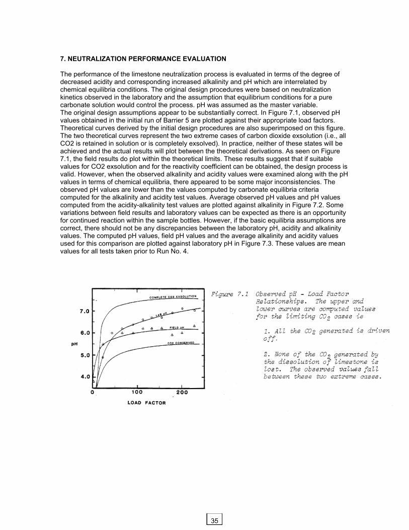
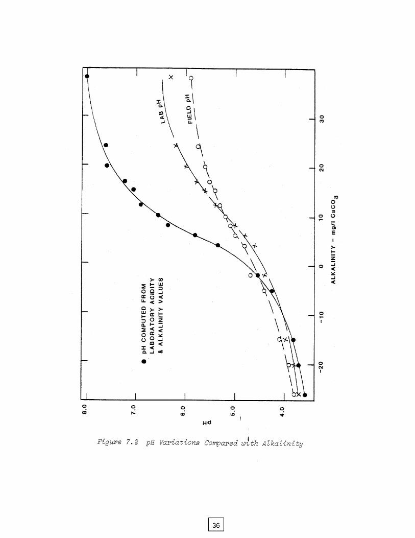
7. NEUTRALIZATION PERFORMANCE EVALUATION The performance of the limestone neutralization process is evaluated in terms of the degree of decreased acidity and corresponding increased alkalinity and pH which are interrelated by chemical equilibria conditions. The original design procedures were based on neutralization kinetics observed in the laboratory and the assumption that equilibrium conditions for a pure carbonate solution would control the process. pH was assumed as the master variable. The original design assumptions appear to be substantially correct. In Figure 7.1, observed pH values obtained in the initial run of Barrier 5 are plotted against their appropriate load factors. Theoretical curves derived by the initial design procedures are also superimposed on this figure. The two theoretical curves represent the two extreme cases of carbon dioxide exsolution (i.e., all CO2 is retained in solution or is completely exsolved). In practice, neither of these states will be achieved and the actual results will plot between the theoretical derivations. As seen on Figure 7.1, the field results do plot within the theoretical limits. These results suggest that if suitable values for CO2 exsolution and for the reactivity coefficient can be obtained, the design process is valid. However, when the observed alkalinity and acidity values were examined along with the pH values in terms of chemical equilibria, there appeared to be some major inconsistencies. The observed pH values are lower than the values computed by carbonate equilibria criteria computed for the alkalinity and acidity test values. Average observed pH values and pH values computed from the acidity-alkalinity test values are plotted against alkalinity in Figure 7.2. Some variations between field results and laboratory values can be expected as there is an opportunity for continued reaction within the sample bottles. However, if the basic equilibria assumptions are correct, there should not be any discrepancies between the laboratory pH, acidity and alkalinity values. The computed pH values, field pH values and the average alkalinity and acidity values used for this comparison are plotted against laboratory pH in Figure 7.3. These values are mean values for all tests taken prior to Run No. 4.

Owner

36

Owner

37

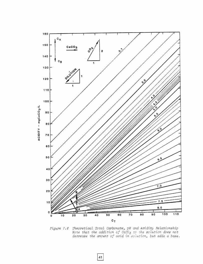
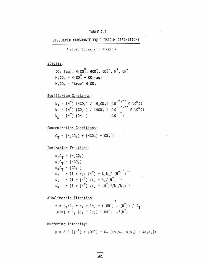
Carbonate System Equilibria: The relationships between pH, acidity and alkalinity are described by carbonate systems equilibria. Table 7.1 and Figure 7.4 identify the governing species and their relationship to one another in the carbonate equilibrium system. The alkalinity and acidity in the reactions are measured by titrating the water samples with an acid or base to the appropriate end point. The titration end points correspond to the equivalence points, x, y and z in Figure 7.4 The equivalence points define the Acid or Base Neutralization Capacity (ANC or BNC). The equations in Table 7.1 define the theoretical acid-base neutralization capacities of the carbonate systems. Alkalinity and acidity are measures of the proton excess or deficiency of a solution with respect to a reference proton level (Ct). Titrations taken to the equivalence points f = 0 and f = 1 give the alkalinity and acidity values of a sample from which Ct is obtained as the difference in the titration values between the two equivalence points. Point y on Figure 7.4 is the phenolphthalein end point. It represents the point at which the solution's ANC is capable of neutralizing an acid concentration equal to the Ct of the solution. Point x represents the end point of the alkalinity determination by "Standard Methods" (22). At this point the solution has no acid neutralization capacity. A negative ANC is common for AMD. The amount of base required to bring the solution to f = 0 (End Point x) is termed the mineral acidity, or, equivalently, free acidity or negative alkalinity. In this range, the solution is highly ionized and H+ added will remain disassociated; a characteristic of a "Strong Acid". In contrast, a "weak" acid is only partially ionized. Aqueous CO2 (H2CO3) acts like a weak acid and the resulting acid concentration is governed by the equilibrium constants given in Table 7.l. The relationship of concentrations of alkalinity, acidity and total carbonate species (Ct) are independent of temperature, pressure and some selected changes in the solutions chemical composition. Graphs of pH contours can be constructed using these concentrations (Ct, Alk, Acy) which can be used to investigate equilibrium conditions. On Figure 7.5 Alkalinity is plotted as a function of Ct as derived from the equations in Table 7.l. Similarly, Figure 7.6 is a plot of Ct versus Acidity. On these graphs, the addition or removal of base, acid, C02, CaCO3 or dilutions of the solution is a vector quantity. The problems of reconciling the test data with equilibrium theory can be illustrated by plotting a typical neutralization result on Figures 7.5 and 7.6. For example, for a lab pH of 6.0 on Figure 7.3, we obtain the following average test results: Alkalinity = 20 mgl Acidity = 2 mgl CT= 22 mgl However, when alkalinity is plotted against Ct on Figure 7.5 (point A) and acidity against Ct on Figure 7.6, a pH value of 7.5 is obtained rather than the actual test value of 6.0. In order to move the plotted Point A from the 7.5 contour to the test 6.0 contour, the addition of an acid or C02 concentration is required in accordance with the vector diagrams on the graphs. In the case of our example a vertical translation of the axis by 15 mgl is necessary to reconcile the test values. This indicates that the solution contains an acid other than that derived from the H+ ion and its presence is not being detected by the acid and alkalinity test values when they are related to the pH test value.

The discrepancy between the lab test values themselves and with neutralization theory created difficulty in analyzing the results of the first 3 runs. In order to resolve this problem, an expanded testing program was proposed, which included field testing for alkalinity and acidity.

Owner

40

Owner

41

Owner

42

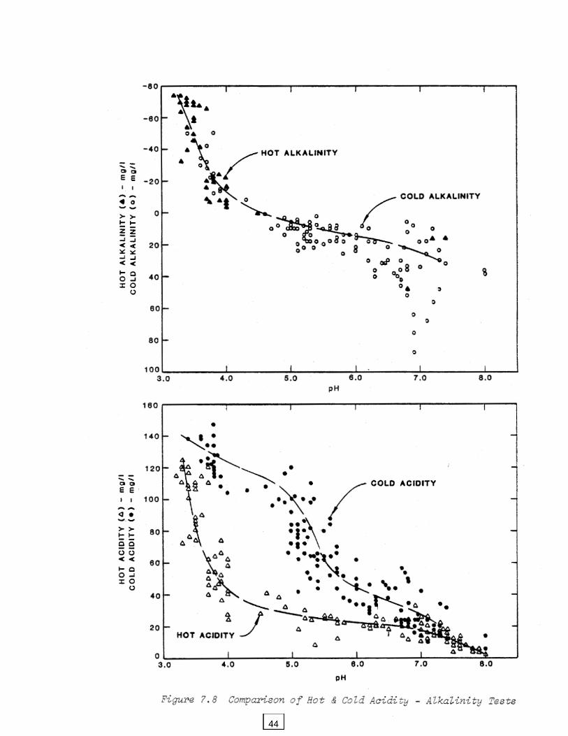
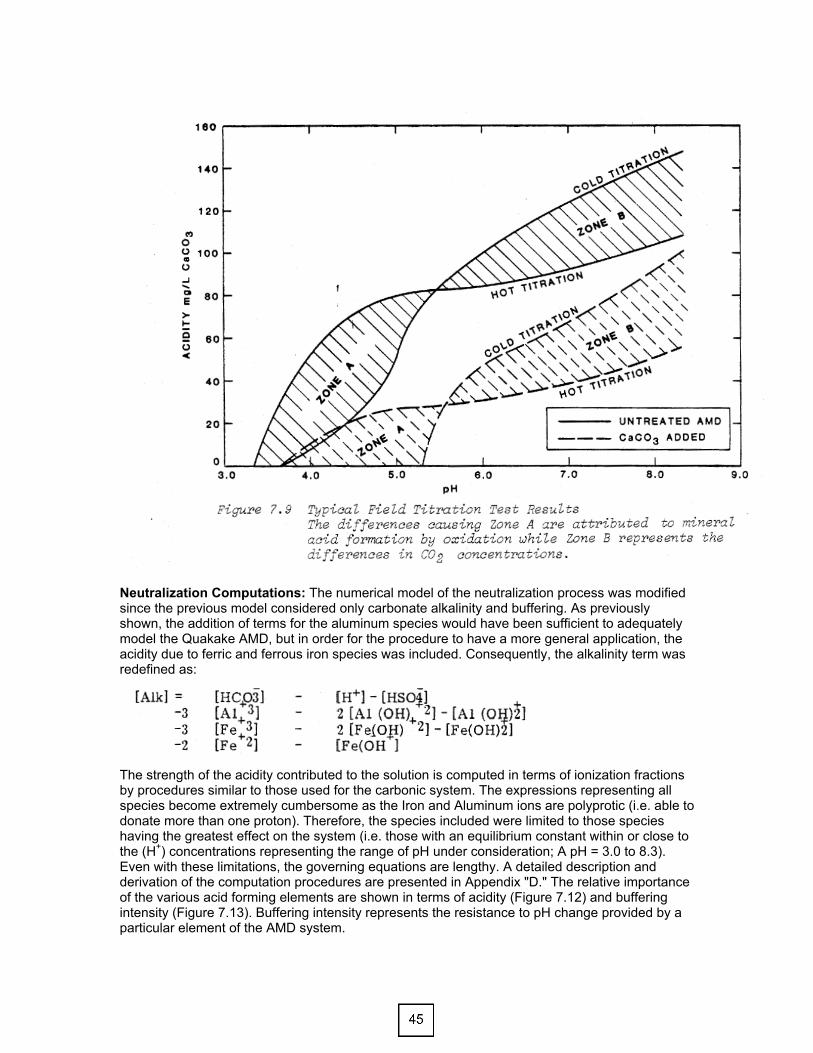
Field Titration Results: All the field titration tests were performed immediately after the samples were obtained. Care was taken to minimize CO2 losses caused by overhandling and mixing. Two types of titration were performed. First, a sample was titrated before the AMD could change temperature ("Cold" titration). A second sample was boiled ("Hot" titration) in accordance with Standard Methods (phenolphthalein acidity at boiling temperature). The boiling drives off all the free carbon dioxide and promotes the hydrolysis of iron and aluminum compounds. A relative measure of the carbon dioxide content is obtained from the difference between the hot and cold acidity titrations (amounts). Plots of the "Hot" and "Cold" titration results are presented in Figure 7.8. As expected, the "Cold" acidity values were much higher than the "Hot" values due to the aqueous carbon dioxide. However, the alkalinity titrations were not expected to show a large increase in mineral acidity. The high "Hot" acidity levels at pH's greater than 5.0 were unexpected as well. A typical set of titration curves, presented in Figure 7.9, illustrates the effects of the carbon dioxide content and mineral acidity. The increase in mineral acidity is attributed to aluminum hydrolysis since iron levels, generally l.0+ mg/l, could not have caused the increased mineral acidity through ferrous-ferric oxidation. The "Hot" acidity values for Run No. 4 are compared with the acidity curve computed for 13 mgl of aluminum in Figure 7.10. As can be seen from this, the acidity beyond the strong (mineral) acid range is caused primarily by partially disassociated aluminum species acting as a weak acid. Figure 7.11 suggests why the acidity caused by the aluminum species was not identified prior to Run No. 4. The low laboratory acidity values, beyond pH = 5, led to the assumption that, once the mineral acidity was neutralized, the remaining acidity would be predominately CO2 acidity. It was also assumed that the iron and aluminum contributed primarily mineral acidity which was largely converted to a precipitate beyond pH = 5.5. The results of the field titrations in Run No. 4 show these assumptions to be incorrect, indicating that the chemical evaluation of the neutralization process is more complex than previously assumed.

Owner

44

Neutralization Computations: The numerical model of the neutralization process was modified since the previous model considered only carbonate alkalinity and buffering. As previously shown, the addition of terms for the aluminum species would have been sufficient to adequately model the Quakake AMD, but in order for the procedure to have a more general application, the acidity due to ferric and ferrous iron species was included. Consequently, the alkalinity term was redefined as:

The strength of the acidity contributed to the solution is computed in terms of ionization fractions by procedures similar to those used for the carbonic system. The expressions representing all species become extremely cumbersome as the Iron and Aluminum ions are polyprotic (i.e. able to donate more than one proton). Therefore, the species included were limited to those species having the greatest effect on the system (i.e. those with an equilibrium constant within or close to the (H+) concentrations representing the range of pH under consideration; A pH = 3.0 to 8.3). Even with these limitations, the governing equations are lengthy. A detailed description and derivation of the computation procedures are presented in Appendix "D." The relative importance of the various acid forming elements are shown in terms of acidity (Figure 7.12) and buffering intensity (Figure 7.13). Buffering intensity represents the resistance to pH change provided by a particular element of the AMD system.

Owner

46

Owner

47

Owner

48