Tamaki, K., Suyehiro, K., Allan, J., McWilliams, M., et al., 1992 Proceedings of the Ocean Drilling Program, Scientific Results, Vol. 127/128, Pt. 2 74. PERFORMANCE OF THE OCEAN BROADBAND DOWNHOLE SEISMOMETER AT SITE 794 1 Toshihiko Kanazawa, 2 Kiyoshi Suyehiro, 3 Naoshi Hirata, 4 and Masanao Shinohara 4,5 ABSTRACT The ocean broadband downhole seismometer (OBDS) was successfully emplaced in Hole 794D in the Japan Sea during ODP Leg 128, and OBDS data were obtained continuously aboard JOIDES Resolution during a 60-hr period of real-time observation. During the real-time observation, air-gun profiling was done around Hole 794D using nine ocean-bottom seismometers (OBSs). The OBDS successfully observed air-gun signals from the seismic profiles, five local earthquakes, and an earthquake in Burma (m b 5.4). Signal-to-noise ratios of air-gun signals and local earthquakes observed by the OBDS are higher by over 20 dB than those observed by OBS. The epicentral distance of Burma earthquake was 38.99° to the OBDS. The OBDS could record P, S, and some surface waves from this teleseismic event with good signal-to-noise ratio for both the vertical and horizontal components. Broadband seismic noise spectra (5 m-30 Hz) in the ocean region were revealed for the first time by the OBDS observation. The noise level falls between the two levels of noisy and quiet conditions on land above 10 s. The noise level increases toward longer period. Signals from earthquakes larger than m s = 6 at 30° distance would rise above noise at an 100-s period. Following the real-time observation, an OBDS seafloor recorder was installed and operated for 30 days in event detection mode and time window mode. There was no triggered event. Very long-period data of 1-hr sampling showed only gradual variations without abrupt steplike changes. This indicates that the clamping we used for the OBDS sensors in the hole was sufficiently stable for such a long-term broadband observation. The results obtained in this paper strongly suggest that a broadband downhole seismometer performs well and is dispensable for constructing broadband digital seismograph networks on the ocean floor. INTRODUCTION Observational seismology has entered a new era with the use of high-performance broadband digital seismographs. Land seismic net- works enjoy this technical advance and have been improving their instrumentation toward wide dynamic range and frequency band, with easy data access observation (e.g., IRIS, GEOSCOPE). The new set of data from these observations advances high-resolution seis- mological studies of the Earth's interior. It has been noted, however, that this new observational window is still limited spatially in the sense that these networks include little of Earth's surface that is covered by water. There are, however, many difficulties in setting uppermanent seismic stations under the sea. These difficulties include the following: (1) Station environment, whether seafloor or borehole observation is required. Sta- tion design is also important, whatever the environment. Even if island observations prove to be adequate, vast areas of open ocean will remain (e.g., in the northwestern Pacific). (2) Sustaining stable long-period observation. (3) Retrieving data. (4) Supplying power. Resolution of these difficulties varies depending on the objectives. More importantly, we lack observational long-period data on which to base our discussion, except for the pioneering experiment of the Columbia-Point Arena Ocean-Bottom Seismic Station (Sutton et al., 1965, 1989). About 7 yr after the last attempted ocean sub-bottom seismic observation (Duennebier, Stephen, et al. (1987c), a new-generation seismic experiment to emplace an ocean broadband downhole seis- mometer (OBDS) was successfully conducted on Ocean Drilling 1 Tamaki, K., Suyehiro, K., Allan, J., McWilliams, M., et al., 1992. Proc. ODP, Sci. ‰swto, 127/128, Pt. 2: College Station, TX (Ocean Drilling Program). 2 Laboratory for Earthquake Chemistry, Faculty of Science, the University of Tokyo, 7-3-1 Hongo, Bunkyo-ku, Tokyo 113, Japan. 3 Ocean Research Institute, the University of Tokyo, 1-15-1 Minamidai, Nakano-ku, Tokyo 164, Japan. 4 Department of Earth Sciences, Faculty of Science, Chiba University, 1 -33 Yayoi-cho, Chiba 260, Japan. 5 Present address: Ocean Research Institute, the University of Tokyo, 1-15-1 Minami- dai, Nakano-ku, Tokyo 164, Japan. Program (ODP) Leg 128 in the Japan Sea (Ingle, Suyehiro, et al., 1990). The borehole instrument was installed at 714.5 m below seafloor (mbsf) within a basalt section near the bottom of Hole 794D. The water depth was 2807 m. Briefly, the experiment was intended to initiate a seismic broad- band observation in the backarc basin of the northern Japan Plate subduction zone to obtain seismic information of the hitherto un- probed crust and upper mantle there. Then, a long-term observation was necessary to capture natural earthquakes larger than moderate size. The seismic sensor is a modified version of a Guralp CMG-3 three-axis feedback-type accelerometer with six-channel outputs of DC-to-30 Hz low-gain and 10 m-to-30 Hz high-gain acceleration signals. The analog signals are digitized by a 16-bit A/D converter at 80 Hz/ch sampling rate and telemetered uphole through the logging cable. Our experiment during Leg 128 consisted of two phases; first, to receive the signals aboard JOIDES Resolution to conduct real-time observation and, second, to connect the logging cable to the seafloor recording system specially constructed for this experiment and deploy it for a long-term observation. During the first phase, an air-gun firing experiment was conducted to detail the crustal structure, including anisotropy together with observation using an ocean-bottom seis- mometer (OBS) array (Hirata et al., this volume; Shinohara et al., this volume). The seafloor recorder for the second phase was designed to record 60 Mb of selected data triggered by earthquakes and for predetermined time windows after appropriate digital filtering. This data set was retrieved after 8 months in May 1990. We shall describe in this paper the characteristics of the seismic signal and noise obtained from this experiment with our focus on long-period data. DATA ACQUISITION Real-Time Experiment A digital broadband (DC-30 Hz) seismometer was emplaced in Hole 794D in the Japan Sea on 26 September 1989. The seismometer housing was locked within the basaltic rock section at 714.5 mbsf at a water depth of 2807 m. Following the installation of the OBDS in Hole 794D, we con- ducted real-time observation (Fig. 1). The purposes of this observa- 1157
Transcript
Tamaki, K., Suyehiro, K., Allan, J., McWilliams, M., et al., 1992Proceedings of the Ocean Drilling Program, Scientific Results, Vol. 127/128, Pt. 2
74. PERFORMANCE OF THE OCEAN BROADBAND DOWNHOLE SEISMOMETER AT SITE 7941
Toshihiko Kanazawa,2 Kiyoshi Suyehiro,3 Naoshi Hirata,4 and Masanao Shinohara4,5
ABSTRACT
The ocean broadband downhole seismometer (OBDS) was successfully emplaced in Hole 794D in the Japan Sea during ODPLeg 128, and OBDS data were obtained continuously aboard JOIDES Resolution during a 60-hr period of real-time observation.During the real-time observation, air-gun profiling was done around Hole 794D using nine ocean-bottom seismometers (OBSs). TheOBDS successfully observed air-gun signals from the seismic profiles, five local earthquakes, and an earthquake in Burma (mb 5.4).
Signal-to-noise ratios of air-gun signals and local earthquakes observed by the OBDS are higher by over 20 dB than thoseobserved by OBS. The epicentral distance of Burma earthquake was 38.99° to the OBDS. The OBDS could record P, S, and somesurface waves from this teleseismic event with good signal-to-noise ratio for both the vertical and horizontal components.Broadband seismic noise spectra (5 m-30 Hz) in the ocean region were revealed for the first time by the OBDS observation. Thenoise level falls between the two levels of noisy and quiet conditions on land above 10 s. The noise level increases toward longerperiod. Signals from earthquakes larger than ms = 6 at 30° distance would rise above noise at an 100-s period.
Following the real-time observation, an OBDS seafloor recorder was installed and operated for 30 days in event detectionmode and time window mode. There was no triggered event. Very long-period data of 1-hr sampling showed only gradualvariations without abrupt steplike changes. This indicates that the clamping we used for the OBDS sensors in the hole wassufficiently stable for such a long-term broadband observation.
The results obtained in this paper strongly suggest that a broadband downhole seismometer performs well and is dispensablefor constructing broadband digital seismograph networks on the ocean floor.
INTRODUCTION
Observational seismology has entered a new era with the use ofhigh-performance broadband digital seismographs. Land seismic net-works enjoy this technical advance and have been improving theirinstrumentation toward wide dynamic range and frequency band,with easy data access observation (e.g., IRIS, GEOSCOPE). The newset of data from these observations advances high-resolution seis-mological studies of the Earth's interior. It has been noted, however,that this new observational window is still limited spatially in thesense that these networks include little of Earth's surface that iscovered by water.
There are, however, many difficulties in setting up permanent seismicstations under the sea. These difficulties include the following: (1) Stationenvironment, whether seafloor or borehole observation is required. Sta-tion design is also important, whatever the environment. Even if islandobservations prove to be adequate, vast areas of open ocean will remain(e.g., in the northwestern Pacific). (2) Sustaining stable long-periodobservation. (3) Retrieving data. (4) Supplying power.
Resolution of these difficulties varies depending on the objectives.More importantly, we lack observational long-period data on whichto base our discussion, except for the pioneering experiment of theColumbia-Point Arena Ocean-Bottom Seismic Station (Sutton et al.,1965, 1989).
About 7 yr after the last attempted ocean sub-bottom seismicobservation (Duennebier, Stephen, et al. (1987c), a new-generationseismic experiment to emplace an ocean broadband downhole seis-mometer (OBDS) was successfully conducted on Ocean Drilling
1 Tamaki, K., Suyehiro, K., Allan, J., McWilliams, M., et al., 1992. Proc. ODP, Sci.‰swto, 127/128, Pt. 2: College Station, TX (Ocean Drilling Program).
2 Laboratory for Earthquake Chemistry, Faculty of Science, the University of Tokyo,7-3-1 Hongo, Bunkyo-ku, Tokyo 113, Japan.
3 Ocean Research Institute, the University of Tokyo, 1-15-1 Minamidai, Nakano-ku,Tokyo 164, Japan.
4 Department of Earth Sciences, Faculty of Science, Chiba University, 1 -33 Yayoi-cho,Chiba 260, Japan.
5 Present address: Ocean Research Institute, the University of Tokyo, 1-15-1 Minami-dai, Nakano-ku, Tokyo 164, Japan.
Program (ODP) Leg 128 in the Japan Sea (Ingle, Suyehiro, et al.,1990). The borehole instrument was installed at 714.5 m belowseafloor (mbsf) within a basalt section near the bottom of Hole 794D.The water depth was 2807 m.
Briefly, the experiment was intended to initiate a seismic broad-band observation in the backarc basin of the northern Japan Platesubduction zone to obtain seismic information of the hitherto un-probed crust and upper mantle there. Then, a long-term observationwas necessary to capture natural earthquakes larger than moderatesize. The seismic sensor is a modified version of a Guralp CMG-3three-axis feedback-type accelerometer with six-channel outputs ofDC-to-30 Hz low-gain and 10 m-to-30 Hz high-gain accelerationsignals. The analog signals are digitized by a 16-bit A/D converter at80 Hz/ch sampling rate and telemetered uphole through the loggingcable. Our experiment during Leg 128 consisted of two phases; first,to receive the signals aboard JOIDES Resolution to conduct real-timeobservation and, second, to connect the logging cable to the seafloorrecording system specially constructed for this experiment and deployit for a long-term observation. During the first phase, an air-gun firingexperiment was conducted to detail the crustal structure, includinganisotropy together with observation using an ocean-bottom seis-mometer (OBS) array (Hirata et al., this volume; Shinohara et al., thisvolume). The seafloor recorder for the second phase was designed torecord 60 Mb of selected data triggered by earthquakes and forpredetermined time windows after appropriate digital filtering. Thisdata set was retrieved after 8 months in May 1990.
We shall describe in this paper the characteristics of the seismicsignal and noise obtained from this experiment with our focus onlong-period data.
DATA ACQUISITION
Real-Time Experiment
A digital broadband (DC-30 Hz) seismometer was emplaced inHole 794D in the Japan Sea on 26 September 1989. The seismometerhousing was locked within the basaltic rock section at 714.5 mbsf ata water depth of 2807 m.
Following the installation of the OBDS in Hole 794D, we con-ducted real-time observation (Fig. 1). The purposes of this observa-
1157
T. KANAZAWA, K. SUYEHIRO, N. HERATA, M. SHINOHARA
45°N
40c
Japan Sea
3 0 0 KM
130°E 135C 140c
Figure 1. Map showing the Japan Sea (after Ingle, Suyehiro, von Breymann et al., 1990). Circled dots denoteLeg 128 sites, and dots show Leg 127 sites. Site 794 was drilled during both legs. Boxed dots indicate DSDP Sites299 through 302. Bathymetry in meters. Blow-up of squared area is shown in Figure 2. Dotted depth contoursindicate Wadati-Benioff zone.
tion were (1) to study the crustal seismic anisotropy in the northernpart of the Yamato Basin, (2) to compare the performance of theseismometer in the hole with that on the ocean bottom, and (3) toknow the orientation of the horizontal sensors of OBDS. We deployedeight analog- and one digital-recording OBSs on two orthogonal linesand did an air-gun profile experiment about Hole 794D (Fig. 2). Itused two 9-L air guns or 17-L air gun on two lines, 70 and 90 km long,and two circles of 9 km (inner circle) and 18 km (outer circle) radius.The shot spacing was about 150 m. The OBDS was positioned at thecenters of the circles and the cross point of the two lines.
The OBDS signals were telemetered to the JOIDES Resolutionvia an electromechanical cable and recorded by the on-board systemat an 80-Hz sampling interval. We successfully recovered the nineOBSs. The local crustal structure derived from the experiment isdescribed in Hirata et al. (this volume) and Shinohara et al. (thisvolume). Unfortunately the digital OBS JRT4H close to Hole 794Ddid not work well. We had planned to use these records for comparingperformance between observations on the seafloor and in the hole.Instead, we used OBS JRT4, an analog-recording OBS deployed closeto Hole 794D, as a replacement for this comparison.
Off-Line Experiment
The seafloor off-line recorder was deployed on the sea bottom nearHole 794D on 29 September 1989, succeeding the 60-hr real-timeexperiment. In May 1990, we recovered the seafloor system, includ-ing a heavy battery unit, without any difficulty. No damage was foundto the recovered unit, although the 400-m nylon rope of 24Φ connected
to the seafloor unit for recovery was slightly abraded by the sedi-ments. No electrical corrosion occurred on the surface of the recov-ered system and the electromechanical cable over about 8 months ofdeployment. Thus, the mechanical design was ideal for the seaflooroff-line recorder and recovery system.
In the recovered 60-Mb tape cartridge, there was no triggeredrecord of an earthquake. In the two-IC memory card of 1 Mb, 35-dayrecords of the very long-period (VLP) signals sampled at 1-hr inter-vals and 245-hr records of the long-period (LP) signals sampled at1-min intervals were recorded. A complete description of the OBDSsystem and the experiments is given in Suyehiro et al. (this volume).
FREQUENCY RESPONSE OF SENSOR ANDOVERALL SYSTEM
OBDS
The seismic sensor of the OBDS is a modified version of a GuralpCMG-3 three-axis feedback-type accelerometer. Each componentwas designed to work within a tilt of ±5° using a leveling mechanism,because ODP holes were expected to be less than 3° from vertical.Each component has two acceleration outputs of DC-to-30 Hz lowgain and 10 m-to-30 Hz high gain. The 10 m-to-30 Hz accelerationsignal is the output of an analog high-pass filter of 10 mHz with again of 15.6 dB to which the low-gain acceleration signal is input.The sensor outputs of the OBDS are fed into a 16-bit analog-to-digitalconverter with a resolution of 0.34 mV at 1 LSB. Figure 3 is a blockdiagram of the sensor. Table 1 lists the sensitivities and cornerfrequencies of sensors. A vertical sensor and a horizontal sensor have
1158
DOWNHOLE SEISMOMETER PERFORMANCE
40°30• N
40°0'
39°50137°40' E 138°0' 138°50'
30 km
Figure 2. Locations of Hole 794D and the OBDS and OBS array. The OBDS and JRT4 were deployed atHole 794D. Filled squares show OBSs. The bathymetry contour interval is 100 m. Air-gun profiles wereconducted along the two perpendicular lines and two circles.
different mechanical structures; therefore, the responses are some-what different especially in the high-frequency end. Figure 4 showsthe frequency responses for a range of 0.3 to 100 Hz and the charac-teristics of the high-pass filter of 10 mHz.
OBS
For comparing OBDS with OBS records in this paper, the charac-teristics of OBS used in the experiment should be known. We willdescribe briefly here the recording system and the typical charac-teristics of the OBS. The OBSs installed around the OBDS wereequipped with three-component velocity sensors of 4.5-Hz naturalfrequency, mounted on a mechanical leveling system (Kanazawa,1986; Matsuda et al., 1986). Movement of the leveling system withtwo orthogonal axes was strongly damped by silicon oil. Outputsignals of the three sensors were amplified with several different gainsto raise the dynamic range and recorded by a direct analog recordingmethod. Using a compact, 90-min cassette tape, a continuous 14-dayrecord was made with an ultra-low tape speed of 0.1 mm/s. Thespecifications and overall frequency response of the OBS JRT4, therecords of which were used for a comparison with the OBDS data,are shown in Table 2 and Figure 5. The frequency response is flat inthe range of 5 to 22 Hz (at -3 dB level). The dynamic range is about40 dB for each recording channel.
HORIZONTAL SENSOR AZIMUTH
We had not designed our system to report its orientation. At thetime of emplacement we controlled the attitude of OBDS within itssensitive range before clamping in place but did not control theorientation of sensors. Therefore, the sensitive azimuths of the hori-zontal sensors were to be estimated from measurement of the recordedpolarity and the amplitude of the air-gun shots in circles around thehole, such as previously performed by Duennebier, Anderson, et al.(1987) and Anderson et al. (1987).
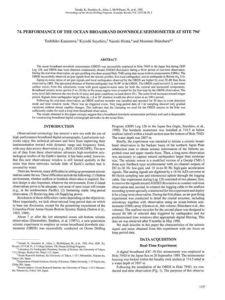
We used the OBDS data of air-gun shots fired in the inner circleduring the real-time observation to determine the azimuths of thehorizontal sensors. Figure 6 shows records of the vertical sensor andthe horizontal sensor, H2, for air-gun shots on the inner circle.Figure 6 also shows the ratio of the maximum amplitude of the initialphases vs. azimuthal angle. The observed amplitude ratio varies witha period of 180°. The minima are at azimuthal angles of 0° and 180°.These show that the H2 sensor is sensitive in the east-west direction.Figure 7 shows records of the H2 sensor for the shots made along theline. The polarity of the first arrival clearly reversed before and afterthe air-gun shots passed over the OBDS, with up direction for shotsin the eastern portion and down direction for those in the westernportion. However, for shots along the north-south line, the polaritychange is ambiguous. And the amplitudes of the first arrivals aresmaller than those in east-west line. All these facts suggest that thehorizontal sensor, H2, was directed toward the west by about 270°.
VERY LONG-PERIOD DATA
Very long-period (VLP) data, the low-gain outputs of the OBDSsensors sampled at 1-hr intervals after the application of a digitalsecond-order high-cut filter of 2 hr, were recorded in the IC memorycard of the seafloor recorder (Fig. 8). The sensor of the OBDS has anautomatic mass-centering function to avoid decreasing the dynamicrange of its output. However, we had disabled the function to avoid amiscalculation of VLP data that would be caused by mass-centering atan 11-min interval. In exchange for a largely reduced dynamic range,reliable VLP data were recorded during the off-line experiment.
Power Consumption of the System
One month after installation of the seafloor system, the VLP beganto fluctuate abruptly and showed a trapezoid-shaped change of 3 daysduration. After records of about 0 count for the next 2 days, VLPrecords ended on the 35th day, when the battery deep-discharge
Figure 3. Block diagram of a modified version of CMG-3 accelerometer. The direct output of the sensor is fed into the 16-bit digitizer as the DC-to-30 Hzlow-gain acceleration signal. In parallel, the direct output is fed into a high-pass filter of 10 mHz with a gain of six and digitized as the 10 mHz-to-30 Hzhigh-gain acceleration signal. Activating DC voltage to calibration coil by a command will check the sensitivity of the sensor.
Table 1. Sensitivity and corner frequency of the OBDS sensor.
Sensor
Vertical sensorV (#V380)
Horizontal sensorHI (#H3133)
Horizontal sensorH2(#H3134)
Channel
Low gainHigh gain
Low gainHigh gain
Low gainHigh gain
Response(Hz)
DC-3010m-30
DC-3010m-30
DC-3010m-30
Sensitivity(V/m•s2)
256615396
270016200
285417124
Table 2. Specifications of the OBS JRT4.
Cornerfrequency (Hz)
44.4
56.0
56.0
Sensor
Amplifier
Recorder
Three components mounted on a gimbal mechanismGeospace GS-1 ID (4.5 Hz, 380 ohm)Sensitivity 0.32 V/kine
Low-noise amplifierVertical component
Horizontal component
High-gain channelLow-gain channel
Gain
90 dB61 dB65 dB
Direct analog recording, 14 days continuouslyTape speed 0.1 mm/s
protection circuit was activated. Vertical and horizontal VLP datashow the same fluctuations with time for which the amounts aredifferent. We think that a voltage drop from the power source causedthe fluctuations. The sensor CMG-3 needs ±12 V to work stably. Otherelectronic parts in the bottom instrument work at ±5 V. Therefore, thevoltage drop affected the sensor first and made it unstable. On the33rd day a serious voltage drop occurred and terminated sensoroperation. By our estimation, the observation period can possibly be
45 days based on the consumption current of 270 mA measured in thelaboratory. In practice, the observation period was only 30 days. Thisshows that the consumption current was on the order of 400 mAduring the off-line observation, which was 1.5 times larger than ourestimation. VLP data of about 10,000 counts on average (Fig. 8)suggest that the outputs of sensors were about 3.5 V DC during theobservation. VLP data show that the mass of a sensor was largely offcenter, which meant that it consumed more electric power than ourestimation and shortened the observation period.
Estimation of Temperature Change and Tilting
The vertical VLP data increased about 14,000 digital counts forthe first 10 days after emplacement. Then it decreased by about 6300digital counts during the next 14 days and became almost stable. Thehorizontal VLP data show similar changes to the vertical ones withalmost the same amount and reversed polarity. Considering a resem-blance between the two components, these long-term variations aresupposed to be caused by temperature changes in the housing.
The OBDS sensor has a temperature coefficient of about-180 ppm/°C. Using this coefficient value, the variations of the VLPdata could be converted to temperature changes inside the housing; atemperature decrease of about 9°C for the first 10 days after theemplacement and an increase of about 4°C during the next 14 days.
Temperature measurements in Hole 395A, provided by the DARPAdownhole seismometer that was emplaced at 609 mbsf, showed a steadyincrease in temperature, about 1°C during 35 days (Becker et al., 1986).Temperature measurements in Hole 581C, by OSSIV which was em-placed about 378 mbsf, showed also a steady increase in temperature,about 6°C during a 64-day period (Duennebier, Cessaro, et al. (1987).Temperature changes in Hole 794D estimated by VLP data were not asteady increase and larger than the changes in Holes 395A and 581C.
The horizontal sensor is sensitive to tilting of the housing or thehole, because horizontal acceleration is indistinguishable from a small
1160
DOWNHOLE SEISMOMETER PERFORMANCE
.O•σ
_Φ<Dcjü<
Φ
180
-1800.1 1 10
Frequency (Hz)100
Vertical
co
•<o
I -20oo<
\
enΦC
180
-1800.1 1 10
Frequency (Hz)100
Horizontal
\
tΦ
•σ
"Q.
< -20
0.0012 0.01 0.1 1Frequency (Hz)
Figure 4. Frequency response of the OBDS sensors. A. The response of the
vertical sensor. B. The response of the horizontal sensor. C. The response of
the high-pass filter.
180
0
180
—
tilt change. As a tiltmeter, the OBDS horizontal sensor works within±24.6 mrad (±1.4°) from vertical with a resolution of 0.75 µrad(corresponds to 1 digital count). The OBDS vertical sensor is notsensitive to tilting as much as the horizontal sensor. Therefore thetilting of the housing or the hole made a contribution to the horizontalVLP variations. We had no measurement of tilt nor temperature in thisstudy, and therefore we can not distinguish the VLP data separatingthe contribution of tilting from that of the temperature change.
Stability of OBDS Emplacement
The method of fixing the instrument in hole is extremely criticalfor such a long-term broadband observation. The OBDS instrumentwas clamped in the basaltic rock section at 715 mbsf by pressingagainst the wall of the hole with an extended pad arm similar to thatof OSS IV. As stated above, the OBDS horizontal sensor has aresolution of 0.75 µrad as a tiltmeter, and a contribution from tiltingof the housing or the hole was contained in the horizontal VLPvariations. However, the VLP data shows only gradual variationswithout abrupt steplike changes. Therefore the tilt variations observedin our experiment were considered to be only gradual ones of whichamounts could not be estimated. Considering this fact, the clampingwe used for the OBDS sensors had sufficient stability.
LOCAL EARTHQUAKES
Hole 794D is situated in the region of aftershocks of the 1983Japan Sea earthquake, M = 7.7. The OBS JRT4 observed 25 earth-quakes during its period of deployment. The OBDS observed fiveearthquakes among these (Table 3). Several of the earthquakes werelocated by the seismological network of Tohoku University.
Figures 9, 10, and 11 show the OBDS acceleration records of theearthquakes, #12, #18, and #21, respectively. For direct comparison,the velocity records of the OBS JRT4 close to Hole 794D are alsoshown in the figures. Figure 12 shows the velocity power spectra ofearthquake #12 observed by the OBDS and the OBS JRT4. The waveshapes of the horizontal sensor of the OBDS are almost similar tothose of the vertical sensor, which is the most impressive charac-teristic of the earthquake records observed by the OBDS. By contrast,the wave shapes of the horizontal sensors of the OBS JRT4 do notresemble those of the vertical sensor because the predominant wavesat about 3.5 Hz were largely excited in the horizontal component ofthe OBS JRT4. Such features are not observed in the records of theOBDS. The excitation of waves of 3.5 Hz is considered to be an effectof the soft sediments on which the OBS JRT4 was emplaced. In therecord of the vertical component of the OBS JRT4, waves of about6 Hz were also excited, but not seen in the OBDS spectra. This mightalso be an effect of the soft sediments.
The predominant frequency of S arrivals observed by the OBDSis 12.6 Hz, which is longer than the approximate 14 Hz of P arrivalsas seen from land observation (Fig. 12). Other characteristics of theOBDS records are a larger dynamic range of wave shapes, muchclearer onsets, better signal-to-noise ratios, and shorter duration of aphase compared to those of the OBS JRT4.
One motivation for emplacing a seismometer beneath the sedi-ments on the ocean bottom was to improve the signal-to-noise ratiofor earthquakes (Carter et al., 1984; Cessaro and Duennebier, 1987).The results of OSS II (clamped at 194-m sub-bottom depth in softsediments) suggest that such an emplacement should avoid the noiseassociated with the sediment/water interface (Carter et al., 1984). Theresults showed that OSS IV appeared to be more sensitive than anOBS placed nearby on the ocean floor, in terms of the signal-to-noiseratio (Cessaro and Duennebier, 1987).
1161
T. KANAZAWA, K. SUYEHIRO, N. HIRATA, M. SHINOHARA
10
Q. 1
Q
3Q. 0.1
δ
0.01
\ OBS JRT4 Vertical Low
Δ - A '
: 500µkina
0.0 0.5 1.0 1.5
Frequency (Log(Hz))2.0
Figure 5. The overall frequency response of the JRT4 OBS plotted for six levelsof velocity.
For our case, during the off-line observation there were no earth-quakes observed, so that we do not have sufficient data. However, theOBDS was more sensitive and had higher quality wave shape DATAthan the OBS JRT4.
AIR-GUN SIGNALS
As stated previously, the crustal structure derived from the air-gunprofiles conducted during the real-time experiment is described inHirata et al. (this volume) and Shinohara et al. (this volume). Thecharacteristics of the record sections of the air-gun profiles observedby the OBDS were also described in Shinohara et al. (this volume).Here, we describe dominant features of air-gun records of the OBDSin comparison with those of the OBS JRT4.
Figures 13 and 14 show air-gun records observed by the OBDSand the OBS, respectively. The OBDS could clearly observe initialarrivals; however, the OBS could not. In the record section of theair-gun profiles, seismograms are plotted side by side which raisesthe signal-to-noise ratio. Therefore, the initial arrivals can be pickedup in the OBS record section. But if we compare a seismogramrecorded by the OBDS with that by the OBS, the OBDS record has alarger signal-to-noise ratio than the OBS record by more than 20 dB.
TELESEISMIC OBSERVATIONS BY OBDS
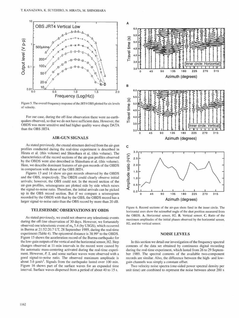
As stated previously, we could not observe any teleseismic eventsduring the off-line observation of 30 days. However, we fortunatelyobserved one teleseismic event of mb 5.4 (by USGS), which occurredin Burma at 21:52:20.7 UT, 28 September 1989, during the real-timeexperiment (Table 4). The epicentral distance is 38.99° to the OBDS.Figure 15 shows the acceleration record of the Burma earthquake forthe low-gain outputs of the vertical and the horizontal sensor, H2. Stepchanges observed at 11-min intervals in the record were caused bythe automatic mass-centering activated during the real-time experi-ment. However, P, S, and some surface waves were observed with agood signal-to-noise ratio. The observed maximum amplitude isabout 3.6 µm/s2. Signals from the earthquake lasted over 100 min.Figure 16 shows part of the surface waves for an expanded timeinterval. Surface waves dispersed from a period of about 40 to 15 s.
I Inner circle: Horizontal |H ) i t i i i>
3.0
4 5 90 135 180 225 270 315
Azimuth (degrees)
45 90 135 180 225
Azimuth (degrees)
270 315
45 90 135 180 225 270 315
Azimuth (degrees)
Figure 6. Record sections of the air-gun shots fired in the inner circle. Thehorizontal axes show the azimuthal angle of the shot position measured fromthe OBDS. A. Horizontal sensor, H2. B. Vertical sensor. C. Ratio of themaximum amplitudes of the initial phases observed by the horizontal sensor,H2, and the vertical sensor.
NOISE LEVELS
In this section we detail our investigation of the frequency spectralcontents of the data set obtained by continuous digital recordingduring the real-time experiment, which lasted from 26 to 29 Septem-ber 1989. The spectral contents of the available two-componentrecords are similar. Also, the difference between the high- and low-gain channels was simply a constant offset.
Two velocity noise spectra (one-sided power spectral density perunit time) are combined to represent the noise between about 200 s
1162
DOWNHOLE SEISMOMETER PERFORMANCE
Table 3. Local earthquakes observed by the OBDS durning the real-timeexperiment (monitored and numbered by OBS JTR4).
Figure 7. Record section obtained by the horizontal sensor, H2, of the air-gunshots fired along the east-west line. The horizontal axis shows the epicentraldistance.
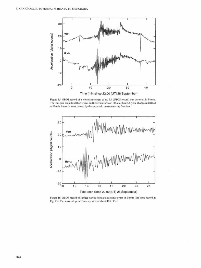
and 30 Hz for the horizontal low-gain component (Fig. 17). For thelower frequency range (up to about 2 s), an average of four spectrabetween 06:00 and 10:00 UT, Sept. 27,1989, each obtained from 8192samples of 2-Hz high-cut filtered data sampled at a 0.125-s interval, isplotted. At higher frequency range, an average of four spectra between21:35 and :38 UT, Sept. 26, 1989, each obtained from 8192 samplesof data sampled at a full rate of 80 Hz, is shown. No air-gun energyappears in Figure 17. The weather condition was fair during this period.
The outstanding peak between 0.1 and 1 Hz consists of two peaksat 0.3 and 0.5 Hz (Fig. 17). These are different from frequencies ofnoise due to ocean waves, namely 0.07-Hz noise generated by wavesacting on coasts and 0.14-Hz noise due to standing ocean waves,originally explained by Wiechert and Longuet-Higgins (Aki andRichards, 1980). We can find the 0.14-Hz peak on the OBDS spectra,suggesting its origin to be due to standing ocean waves (Fig. 17).
If we compare the OBDS noise power spectra with that of noisyand quiet conditions for a typical station on hard basement rock (Akiand Richards, 1980), we find that the OBDS noise level falls betweenthe two levels on land above 10 s (Fig. 17). The noise level increasestoward the longer period. Signals from earthquakes larger than ms =6 at 30° distance would rise above noise at a 100-s period.
Among the few ocean bottom long-period seismic observations(Sutton et al., 1988; Trevorrow et al., 1990; Dozorov and Soloviev,1991), we compare with the results obtained from the Columbia-PointArena Ocean Bottom Seismic Station (OBSS) in Figure 17 (Sutton etal., 1988). Their results are comparable to or quieter than other resultsbelow 10 Hz (Dozorov and Soloviev, 1991). The OBDS noise levelis lower than OBSS above 0.1 Hz. The increase in OBDS noise levelbelow 0.1 Hz is probably due to the system and not representingnatural noise, because OBDS has only acceleration outputs with a
resolution of about 1.2 ×10"7 m/s2, which is equivalent to about 1.9×10²nm/sat0.1 Hz.
Figure 18 represents the spectra in displacement. The displace-ment power density falls at about 43 dB/decade. This figure may becompared with the noise spectra from Marine Seismic System (MSS)and quiet continental sites at Queen Creek, Arizona, and Lajitas, Texas(Adair et al., 1986), and Seismic Research Observatory (SRO) stationon Guam island (GUMO) (Hedlin and Orcutt, 1989). We choseGUMO data for comparison because this station was quieter thanTaiwan and Easter Island stations as discussed by Hedlin and Orcutt(1989), who found that island stations and OBS or MSS noise spectraare comparable between 0.1 and 10 Hz, and thus, seafloor stations arepractical where there are not nearby islands for stations.
The OBDS is quieter than MSS below 0.1 Hz and quieter thanGUMO above about 0.15 Hz. Below 0.1 Hz, island stations show areduction in displacement power, whereas the OBDS does not be-cause of the resolution problem given above. Still at the low-fre-quency band above about 0.01 Hz, the OBDS is capable of capturinglarge global earthquakes or intermediate events at teleseismic dis-tances as exemplified by the teleseismic event record.
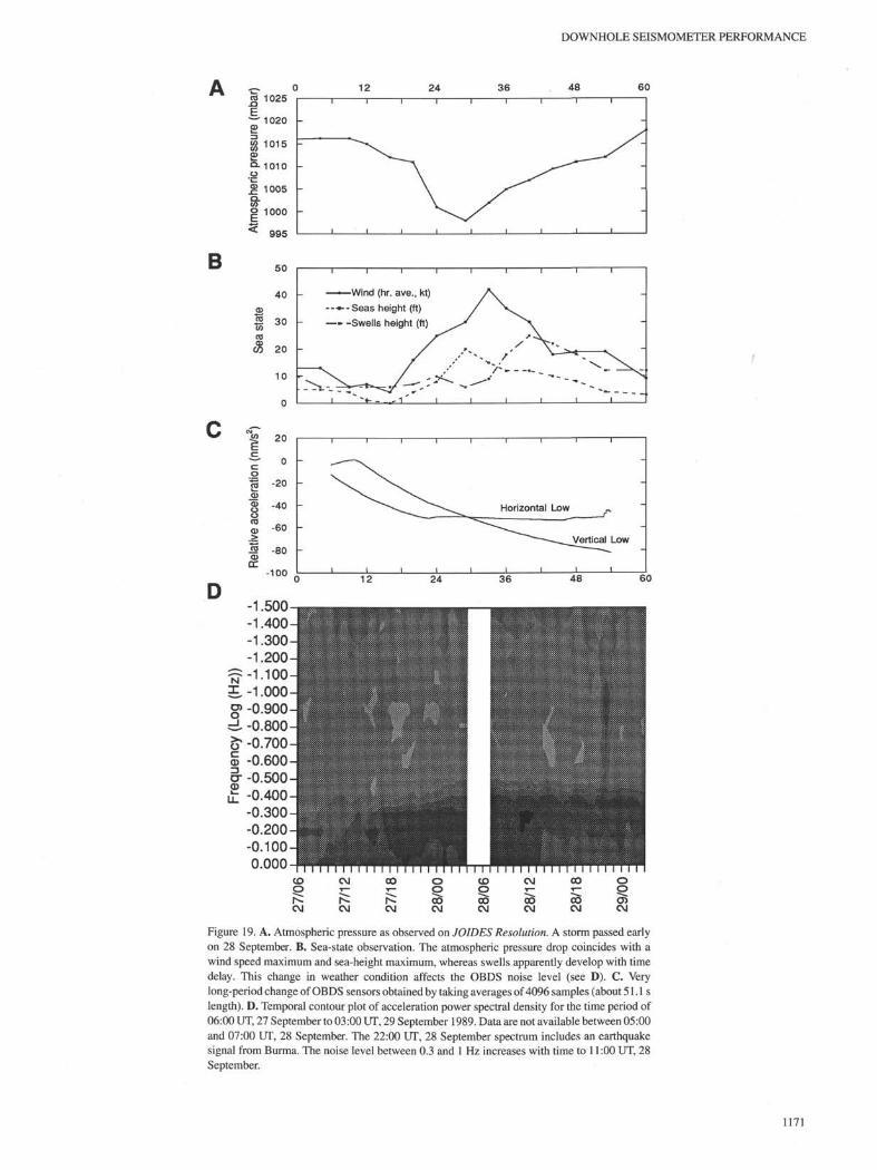
The temporal change of the acceleration power spectral density isshown in Figure 19D. This was obtained by contouring the spectracalculated for 8192 samples at 0.125-s intervals starting at hourintervals from 06:00 UT, 27 September to 03:00 UT, 29 September.A decade change in power spectral density level corresponds to agray-scale level change. The conspicuous spectra at 22:00 UT, 28September is the result of an earthquake (Fig. 15).
When we compare this with the sea state and atmospheric pressure(Fig. 19 A, B), we see that above about 0.3 Hz, the change correspondsto the change in pressure and sea state except for swell height.Apparently, below this frequency, the noise level is not affected bythese factors. Figure 19C was obtained by calculating the mean valuesof 4096 samples at about 51-s intervals and substituting DC offsetscaused by the 11-min mass centering function by interpolations. Thevertical component does not seem to be affected by the weather,whereas the horizontal component seems to have changed its trend ata maximum in atmospheric pressure rate, although its physical rela-tionship is not clear.
CONCLUSIONS
We analyzed the observed records of the OBDS during phase 1, thereal-time observation, and phase 2, the off-line observation, to clarify itsperformance. We also analyzed the observed records of the OBS JRT4,which was emplaced close to the OBDS to compare the performance ofthe OBDS in the hole with the observation from the seafloor.
The following results were obtained in this study.
1. The orientation of the horizontal sensors was successfullydetermined by analyzing the records of air-gun profiles conductedduring the phase 1. The horizontal sensor, H2, was directed towardthe west by about 270°, and HI was directed toward the south.
2. The method of fixing the instrument in hole is extremely criticalfor such a long-term broadband observation. The OBDS instrumentwas clamped in the basaltic rock section at 715 mbsf by pressingagainst the wall of the hole with an extended pad arm. The clampingperformed well with sufficient stability.
3. Comparison between the records of the OBDS and the OBSJRT4 for local earthquakes and air-gun signals shows that the OBDShad higher quality wave shapes and a larger signal-to-noise ratio ofmore than 20 dB greater than that of the OBS.
4. The OBDS could record P, S, and dispersed surface waves with goodsignal-to-noise ratios for the vertical and horizontal components from ateleseismic event of a magnitude nib 5.4 that occurred in Burma onSeptember 28,1989. The epicentral distance was 38.99° to the OBDS.
5. The seismic noise spectrum was revealed for the first time inbroadband (5 m-30 Hz) in the sea region by our OBDS observation.
1163
T. KANAZAWA, K. SUYEHIRO, N. HIRATA, M. SHINOHARA
30000
£ 20000
Oo
5)
a)oo<
10000
-10000
Long-term hourly values (high-cut filtered at 7200 s)
5 10 15 20 25
Time (days since 00:00 [UT] -30September 1989 )
Figure 8. Record section of VLP data for the OBDS sensors.
The noise level falls between the two levels of noisy and quietconditions on a hard basement rock on land above 10 s. Comparisonswith previous islands, seafloor, or borehole observations at frequen-cies above 0.1 Hz showed that the OBDS site was relatively quiet.The noise level increases toward a longer period, which is probablydetermined by the system.
The results obtained in this paper strongly suggest that a broad-band downhole seismometer is a high-performance solution for con-structing broadband digital seismograph networks on the ocean floor.
ACKNOWLEDGMENTS
We thank the staffs and the crews of JOIDES Resolution, Tansei-maru, Kaiko-maru 5, and Wakashio-maru for their contributions tothe experiments. We owe very much to the ODP engineers andtechnicians and Schlumberger engineer aboard JOIDES Resolutionfor Leg 128. We thank all the shipboard scientists, including H. Kinoshita,H. Shiobara, and A. Nishizawa.
REFERENCES
Adair, R. G., Orcutt, J. A., and Jordan, T. H., 1986. Analysis of ambient seismicnoise recorded by downhole and ocean-bottom seismometers on Deep SeaDrilling Project Leg 78B. In Hyndman, R. D., Salisbury, M. H., et al., Init.Repts, DSDP, 78B: Washington (U.S. Govt. Printing Office), 767-781.
Aki, K., and Richards, P., 1980. Quantitative Seismology (Vol. 1): New York(Freeman), 497-498.
Anderson, P. N., Duennebier, F. K., and Cessaro, R. K., 1987. Ocean boreholehorizontal seismic sensor orientation determined from explosive charges.J. Geophys. Res., 92:3573-3579.
Becker, K., Langseth, M. G., and Hyndman, D., 1986. Temperature measure-ments in Hole 395A, Leg 78B. In Hyndman, R. D., Salisbury, M. H., et al.,Init. Repts. DSDP, 78B: Washington (U.S. Govt. Printing Office), 767-781.
Carter, J. A., Duennebier, F. K., and Hussong, D. M., 1984. A comparisonbetween a downhole seismometer and a seismometer on the ocean floor.Bull. Seismol. Soc. Am., 74:763-772.
Cessaro, R. K., and Duennebier, F., 1987. Regional earthquakes recorded byocean bottom seismometers (OBS) and an ocean sub-bottom seismometer(OSS IV) on Leg 88. In Duennebier, F. K., Stephen, R., et al., Init. Repts.DSDP, 88: Washington (U.S. Govt. Printing Office), 129-145.
Dozorov, T. A., and Soloviev, S. L., 1991. Spectra of ocean-bottom seismicnoise in the 0.01-10 Hz range. Geophys. J. Int., 106:113-121.
Duennebier, F. K., Anderson, P. N., and Fryer, G. J., 1987. Azimuth determi-nation of and from horizontal ocean bottom seismic sensors. J. Geophys.Res., 92:3567-3572.
Duennebier, F. K., Cessaro, R. K. and Harris, D., 1987. Temperature and tiltvariation measured for 64 days in Hole 581C. In Duennebier, F. K.,Stephen, R., Gettrust, J. F., et al., Init. Repts. DSDP, 88: Washington (U.S.Govt. Printing Office), 161-165.
Duennebier, F. K., Stephen, R., Gettrust, J. F., et al., 1987. Init. Repts. DSDP,88: Washington (U.S. Govt. Printing Office).
Hedlin, M.A.H., and Orcutt, J. A., 1989. A comparative study of island, seafloor,and subseafloor ambient noise levels. Bull. Seis. Soc. Am., 79:172-179.
Ingle, J. C , Jr., Suyehiro, K., von Breymann, M., et al., 1990. Proc. ODP, Init.Repts., 128: College Station, TX (Ocean Drilling Program).
Jeffreys, H., and Bullen, K. E., 1940. Seismological Tables: British Associa-tion, Gray-Milne Trust.
Kanazawa, T., 1986. Ocean bottom seismometer with low power design. Annu.Meet. Seismol. Soc. Jpn. Abstr., 2:240. (Abstract in Japanese)
Matsuda, N., Fujii, T, and Kinoshita, H., 1986. Pop up ocean bottom seis-mometer with hydrophone system. Annu. Meet. Seismol. Soc. Jpn. Abstr.,2:241. (Abstract in Japanese)
Sutton, G. H., Barstow, N., and Carter, J. A., 1988. Long-period seismic meas-urements on the ocean floor. In Proc. Workshop on Broad-band DownholeSeismometers in the Deep Ocean. Woods Hole Oceanogr. Inst., 126-142.
Sutton, G. H., McDonald, W. G., Prentiss, D. D., and Thanos, S. N., 1965.Ocean-bottom seismic observatories. Proc. IEEE, 53:1909-1921.
Trevorrow, M. V, Yamamoto, T., Turgut, A., Goodman, D., and Badiey, M.,1990. Very low frequency ocean bottom ambient seismic noise and cou-pling on the shallow continental shelf. Mar. Geophys. Res., 11:129-152.
Date of initial receipt: 8 May 1991Date of acceptance: 28 February 1992Ms 127/128B-236
1164
DOWNHOLE SEISMOMETER PERFORMANCE
A 2000
-8000
Time (s)
20 25 30
Time (s)
Figure 9. Records of the earthquake #12 (Table 3). A. Acceleration records from the OBDS. High-gain outputs of vertical and horizontalsensors are shown. B. P-wave acceleration records from the OBDS, with an expanded time scale. C. Velocity records for verticallow-gain output and horizontal outputs, HI and H2, from the OBS JRT4.
8B
-10
-12×10J
5 10 15 20 25 30 35
Time (s)15 20 25 30 35 40 45
Time (s)
Figure 10. Records of the earthquake #18 (Table 3). A. Acceleration records for the high-gain outputs ofvertical and horizontal sensors observed by the OBDS. B. Velocity records of vertical low-gain outputand horizontal outputs, HI and H2, observed by the OBS JRT4. 5 waves are saturated on all traces.
1165
T. KANAZAWA, K. SUYEHIRO, N. HIRATA, M. SHINOHARA
10 15 20
Time (s)15 20 25 30 35 40
Time (s)
Figure 11. The records of the earthquake #21 (Table 3). A. Acceleration records for the high-gain outputsof vertical and horizontal sensors observed by the OBDS. B. Velocity records of vertical high-gain outputand horizontal outputs, HI and H2, from the OBS JRT4. 5 waves on the vertical trace are saturated.
10
1010
Frequency (Hz)
101 10
Frequency (Hz)
Figure 12. The velocity power spectra of earthquake #12 (Table 3). A. Velocity power spectra of the OBDSvertical high-gain output and the JRT4 vertical low-gain output around P-wave arrivals. OBS velocityresponse was assumed flat, so frequency range of 5 to 22 Hz is within 3 dB change (Fig. 5). For direct levelcomparison, OBS curve should be lowered by about 26 dB in power. B. Velocity power spectra of the OBDShorizontal high-gain output and the JRT4 horizontal output, HI, around 5- wave arrivals.
1166
DOWNHOLE SEISMOMETER PERFORMANCE
600
Figure 13. Record of air-gun shot # 160 of the north-south line observed by theOBDS at a distance of 7.99 km. A. Velocity record of the vertical high-gainoutput applied by a 5-Hz high-pass filter. B. The same velocity record with anexpanded time scale.
3.0 3.5
Time (s)
Figure 14. Record of air-gun shot #160 of the north-south line observed bythe OBS at a distance of 7.62 km. A. Velocity record of the vertical low-gainoutput. B. The same velocity record with an expanded time scale.
Table 4. Teleseismic event observed by the OBDS (determinedbyUSGS).
Origin time [UT]HypocenterMagnitudeDistance to OBDSTraveltime from Jeffreysand Bullen table (1940)
9/28 21:52 20.720.313°N98.809°E
mb5.438.99°
P:S:
33 km Burma
8 min. 6 s14 min. 35 s
1167
T. KANAZAWA, K. SUYEHIRO, N. HIRATA, M. SHINOHARA
σ>
-10 -
-200 10 20 30
Time (min since 22:00 [UT] 28 September)
Figure 15. OBDS record of a teleseismic event of mb 5.4 (USGS record) that occurred in Burma.The low-gain outputs of the vertical and horizontal sensor, H2, are shown. Cyclic changes observedat 11-min intervals were caused by the automatic mass-centering function.
-2010 12 14 16 18 20 22
Time (min since 22:00 [UT] 28 September)
Figure 16. OBDS record of surface waves from a teleseismic event in Burma (the same record as
Fig. 15). The waves disperse from a period of about 40 to 15 s.
1168
DOWNHOLE SEISMOMETER PERFORMANCE
0.01 0.1 1
Frequency (Hz)10
io1l l ü H —i—t-t-t0.1
Frequency (Hz)Figure 17. Velocity power spectral density per unit time (one-sided) obtained from OBDS horizontal low-gain component. A.OBDS curve for frequencies below about 0.5 Hz is the mean of four 1022-s-long data sets between 06:00 and 10:00 UT on27 September 1989. The mean of four 102-s-long data sets between 21:35 and 21:38 UT on 26 September is plotted forfrequencies above about 0.5 Hz. Also shown are typical land noise curves from Aki and Richards (1980). Dotted curve isvertical-component spectra of OBSS at a quiet period from Sutton et al. (1988). B. Expanded plot of A showing three spectralpeaks. The leftmost peak is at about 0.14 Hz.
1169
T. KANAZAWA, K. SUYEHIRO, N. HIRATA, M. SHINOHARA
10*
NX
QCO
α_Q)
ECDü
Q .W
b
10
Frequency (Hz)Figure 18. Displacement power spectral representation of Figure 17. Displacement power decay is about 43 dB/decade. Also shown for comparison are MSS,Queen Creek, and Lajitas from Adair et al. (1986), and GUMO from Hedlin and Orcutt (1989).
Figure 19. A. Atmospheric pressure as observed on JOIDES Resolution. A storm passed earlyon 28 September. B. Sea-state observation. The atmospheric pressure drop coincides with awind speed maximum and sea-height maximum, whereas swells apparently develop with timedelay. This change in weather condition affects the OBDS noise level (see D). C. Verylong-period change of OBDS sensors obtained by taking averages of 4096 samples (about 51.1slength). D. Temporal contour plot of acceleration power spectral density for the time period of06:00 UT, 27 September to 03:00 UT, 29 September 1989. Data are not available between 05:00and 07:00 UT, 28 September. The 22:00 UT, 28 September spectrum includes an earthquakesignal from Burma. The noise level between 0.3 and 1 Hz increases with time to 11:00 UT, 28September.