DYNAMIC PORTFOLIO ALLOCATION, THE DUAL THEORY OF CHOICEAND PROBABILITY DISTORTION FUNCTIONS
BY
MAHMOUD HAMADA, MICHAEL SHERRIS AND JOHN VAN DER HOEK
ABSTRACT
Standard optimal portfolio choice models assume that investors maximise theexpected utility of their future outcomes. However, behaviour which is incon-sistent with the expected utility theory has often been observed.
In a discrete time setting, we provide a formal treatment of risk measuresbased on distortion functions that are consistent with Yaari’s dual (non-expectedutility) theory of choice (1987), and set out a general layout for portfolio optimi-sation in this non-expected utility framework using the risk neutral computa-tional approach.
As an application, we consider two particular risk measures. The first oneis based on the PH-transform and treats the upside and downside of the riskdifferently. The second one, introduced by Wang (2000) uses a probability dis-tortion operator based on the cumulative normal distribution function. Bothrisk measures rank-order prospects and apply a distortion function to the entirevector of probabilities.
KEYWORDS
Portfolio allocation, dual theory, probability distortion, equilibrium pricing.
1. INTRODUCTION
This paper considers the dynamic optimal consumption and portfolio selectionproblem, in a discrete-time setting and using a non-expected utility setting. Themajority of portfolio choice models assume that preferences are representedby a von Neuman-Morgenstern utility function and individuals choose amongrisky alternatives so as to maximise the expectation of the utility of possibleoutcomes. Although the expected utility model has long been the standard forchoice under uncertainty, questions have been raised concerning its validity, andbehavior patterns which are systematic, yet inconsistent with expected utilitytheory have often been observed as in the Allais paradox (1953 [1]) and Kahne-man & Tversky (1979 [11]). Fishburn (1988 [6]) surveys the reasons why the
expected utility hypothesis fails. Camerer (1989 [3]) carries out empirical testsof several generalized models of utility theory. Yaari (1987 [24]) developed adual theory of choice under risk where the roles of probabilities and paymentsare interchanged, so the wealth utility function is replaced by a probability dis-tortion function. Some of the expected utility related paradoxes are resolvedin the dual theory. The rank dependent utility model introduced by Quiggin(1982, [15]) can be viewed as an extension of both the expected utility and thedual utility models where both the cumulative distribution function and the out-comes are distorted. The idea of the rank dependent utility model is to rank-order prospects and apply a distortion function (called weighting function byQuiggin [15]) to the entire vector of probabilities and the utility function tothe outcomes.
Recently, there has been development in a non-expected utility framework.Wang (1995 [20], 1996 [19]) proposes calculating insurance premiums by apply-ing the proportional hazards transform to the decumulative distribution func-tion, thereby introducing a new risk measure. This new measure turns out tobe consistent with Yaari’s dual theory of choice. Wang (2000 [22]) also usesa different class of distortion operators to recover the Black-Scholes formula.Van der Hoek and Sherris (2001 [18]) introduce a new class of risk measuresfor asset allocation which is based on the distortion function approach to insur-ance risk.
Empirically, there is evidence to support non-expected utility model. Indeed,Bufman and Leiderman (1990 [2]) use Israeli data between 1978 and 1986 totest an intertemporal consumption-investment model introduced by Epsteinand Zin (1989 [5]) that uses Kreps-Porteus (1978 [13]) non-expected utilitypreferences. They find evidence to reject the expected utility model and acceptthe non-expected utility one. Their results differ from those of Epstein andZin (1989b [4]) and Giovannini and Jorion (1989 [7]) who took data from thetranquil postwar US economy. This suggests that a non-expected utility modelmay perform better in a volatile economy. The results of the empirical tests ofthe same model using French data from 1960 to 1994 conducted by Koskievic(1999 [12]) support those of Bufman and Leiderman (1990 [2]).
This paper is organised as follows. In section 2, we present the concept ofrisk aversion for non-expected utility and illustrate the idea of using a distortionfunction to price risk. New objective for asset allocation is set in non-expectedutility framework. Section 3 provides a formal treatment of risk measuresbased on probability distortion. New class of risk measures for portfolio selec-tion based on the proportional hazards transform, proposed by van der Hoekand Sherris (2001 [18]) is then reviewed and extended to the multinomial case.This is the first step in setting out a general scheme for dynamic asset allocationwhen the risk measure is based on a distortion function. Some other proper-ties, useful for the optimisation, are developed along the way. In section 4 wederive a dual utility theory equilibrium pricing formula for market securitiesand propose to solve the optimal portfolio problem using the risk neutral com-putational approach when the investor behaviour is modeled by this new class
188 M. HAMADA, M. SHERRIS AND J. VAN DER HOEK
8464-05_Astin36/1_08 29-05-2006 15:17 Pagina 188
of risk measures. In section 5, we extend the previous framework from singleperiod to multi-period. In section 6, some numerical examples for asset allo-cation are provided. The conclusion highlights some further developments.
2. NON-EXPECTED UTILITY THEORY
2.1. Risk aversion in utility theory and its dual
Decision makers with a von Neumann-Morgenstern utility function are saidto be risk averse if they prefer to have the expected value of a gamble ratherthan facing the gamble itself, i.e. For all gambles X with �(X ) = 0 and positivevariance, and for a level of wealth W, U(W ) > EU(W + X ).
It can be proved (see Ingersoll [10]) that decision makers are risk averse ifand only if their von Neumann-Morgenstern utility function of wealth isstrictly concave. Moreover, the level of risk aversion is measured by the degreeof concavity of the utility function. Locally, this is determined by Arrow-Pratt’s
absolute risk aversion index: A(W) = ( )( )
u wu w
�
�. The larger the index, the more risk-
averse the agent.To induce a risk-averse individual to undertake a fair gamble, a compen-
satory risk premium Pc(X ) has to be offered. Or dually, to avoid a presentgamble, a risk averse individual would be willing to pay an insurance risk pre-mium Pi (X ). These risk premiums are depicted as follows:
� [U(W + Pc(X ) + X )] = U(W)
� [U(W + X )] = U(W – Pi(X ))
The amount W – Pi (X ) is the amount which, when received with certainty, isconsidered by the individual as good as W + X. It is called the certainty equiv-alent of the gamble W + X.
In the expected utility theory, suppose that an individual must choose amonglotteries with at most n outcomes x1, x2, …, xn, with respective probabilities p1,p2, …, pn, then there exists a utility function U such that this individual’s choicecriterion is to maximise
� U X p U x u X dPw wi ii
n
W1
= ==
#!] ^ ]^ ]g h gh g6 @
Note that this objective function is linear in probabilities and distorts the payoffs.In the dual theory of choice introduced by Yaari [24], the certainty equiva-
lent to X ≥ 0 is defined as:
X gP0
=3#] g (SX (t))dt
DYNAMIC PORTFOLIO ALLOCATION 189
8464-05_Astin36/1_08 29-05-2006 15:17 Pagina 189
where g is a “dual utility” or a distortion function (continuous and non-decreas-ing) g : [0,1] → [0,1] with g(0) = 0 and g(1) = 1, applied to the probability decu-mulative distribution:
SX (t) = Pr[X > t ]
This general form of P(X) is valid for continuous and discrete time cases,where the integral sign will be a summation sign in a discrete case, and theappropriate formula is developed later. If X is a non-negative random variablerepresenting a loss amount then P(X) is the certainty equivalent of the risk X.In the dual theory, given a choice among risky prospects, the agent would preferrisks having the greatest certainty equivalent.
It can be proved (see Yaari [24]) that the investor is risk averse if and onlyif g is convex. An intuitive interpretation of this property follows in the casewhen g is differentiable:
X g S t dt tg S t d tP X X X00
= =33
� F##] ]^ ]^ ]g gh gh gassuming that tg[SX (t)] → 0 as t → ∞. Recall that:
� X td tX0
=3
F# ] g6 @Comparing P(X) to � [X ], P(X) can be thought of as a corrected mean of Xwhere the payment t receives a weight g�(SX (t)) ≥ 0. Note that these weights sumup to 1, i.e. g�# (SX (t))dFX (t) = dt
d# [–g(SX (t))]dt = g(1) – g(0) = 1.If g is convex, then
Therefore, the weight assigned to a high outcome is less than the weightassigned to a low outcome. Hence, by distorting the probabilities with a con-vex function, agents behave pessimistically, in the sense that they assign highprobability to bad outcomes and low probability to good outcomes.
The comparison of risk aversion in this framework is naturally based onthe convexity of the function g representing the agent’s preference function. Themore convex the function g, the more risk averse the agent. The dual Arrow-Prattrisk aversion would be in this case ( )
( )g pg p
�
� for 0 < p < 1, as defined in Yarri (1986 [23]).In the sense of Ross (1981 [17]), agents are strongly more risk averse, if theyrequire a larger compensation for any mean preserving spread in their prospects,even if the initial situation is not one of perfect certainty. Risk aversion mea-surement in the sense of Yaari (1986 [23]) and Ross (1981 [17]) are discussedin Röel (1985 [16]).
To sum up, while risk aversion in utility theory is measured by the utilityfunction, in the dual theory, it is measured by the probability distortion function.
190 M. HAMADA, M. SHERRIS AND J. VAN DER HOEK
8464-05_Astin36/1_08 29-05-2006 15:17 Pagina 190
The choice of the distortion function g determines the properties of the cer-tainty equivalent.
In the literature, Wang (1996 [20]) proposes a general class of distortion oper-ators to use in pricing insurance premiums. When the distortion function is apower function, i.e., g(x) = xr, the mapping
SX(t) → g(SX(t))
is called the PH-transform. Applications and implementation of the PH-trans-form in insurance is discussed in Wang (1998 [21]). Although the PH-transformenjoys desirable properties in insurance pricing, it cannot be applied to assetsand liabilities simultaneously. Wang (2000 [22]) proposes another class of dis-tortion operators
ga( p) = F[F–1( p) + a ]
where F( p) = ep
p2
1x2
2
3-
-# dx is the standard normal cumulative distribution
function and shows how the mean of the distorted decumulative distributioncan be used as another alternative to the risk-neutral valuation in asset pricing.Van der Hoek and Sherris (2001 [18]) introduced another framework for pricingasset and liabilities, based on distortion of the probability distribution. They usetwo different distortion operators, g and h to allow a different pricing of theupside and downside of the risk. The specification of g and h is not given,thereby allowing for a general pricing framework. In the following, we shall con-sider the certainty equivalent in discrete-time, then overview the risk measureintroduced by van der Hoek and Sherris (2001 [18]), develop new propertieswhich are useful for optimisation, and use these results to solve the optimalportfolio problem.
2.2. New Objective for Asset Allocation
In multi-period asset allocation, investors are faced with a series of decisionswhere at the beginning of each period, they have to choose the optimal amountof consumption and investment. The optimal consumption level Ct at time tis a risky prospect. Formally, Ct, t = 0,…,T is a non-negative and boundedrandom variable defined on some probability space. By virtue of Theorem 2in Yaari ([23]), the scheme (C0, C1,…,CT) is preferred to (C�0, C�1,…,C�T) if andonly if there exists an increasing continuous function U : Rn
+ → R+ such that:
U (H(C0), H(C1),…, H(CT)) ≥ U(H(C�0), H(C�1),…,H(C�T ))
The investor chooses the consumption stream that maximises an increasing func-tion of the certainty equivalent of consumption at each period.
DYNAMIC PORTFOLIO ALLOCATION 191
8464-05_Astin36/1_08 29-05-2006 15:17 Pagina 191
In what follows, we choose
:
, , ...,
U R R
x x x xbn1 2
"
7
n+
i
+
i!^ hwhere 0 < b ≤ 1 is the time preference factor. The consumption-investmentproblem can be reformulated as follows:
t. .
,
�
Max H C
s t Wr
C
C t T
b
1
0 0
, ,...,C C Ctt
tt
t
Q
0
0 0
T0 1
6$ !
=+
=
=
T
T
t!
!
^
]h
g=6
G@
Z
[
\
]]]
]]]
(2.1)
where W0 is initial wealth and r is a constant interest rate, that can be extendedto be varying with time and states of nature. Q is the risk-neutral probabilitymeasure under which the underlying security process is martingale. The objec-tive function is not as tractable as in the expected utility theory. This is becauseit depends on the order of consumption. In the following section, we developan expression for the discrete time case.
3. ASSET ALLOCATION IN SINGLE-PERIOD
3.1. Dual Theory Equilibrium Pricing
In the dual utility theory the consumer-investor problem for a single-periodusing the rank-ordered optimisation framework is
0
,
max
�
C H C
C C
W C r C
subject to
and
b
0
11
,C C
Q
0 1
0 1
0 1
0 1
$
+
= ++
^ h
6 @
Z
[
\
]]]
]]]
(3.1)
where C0 and C1 are consumption at time 0 and 1 respectively, W0 is initialwealth, b is a time discount factor and r is a constant interest rate, that can beextended to be varying with time and states of nature. Q is the risk-neutralprobability measure under which the underlying security process is martingale.
Suppose that C*0 and C*
1 are solution to (3.1). Perturb the consumption C*0 in
such a way that the consumer consumes less than C*0 in order to invest in a
security j whose price at time 0 is xj. This translates to
192 M. HAMADA, M. SHERRIS AND J. VAN DER HOEK
8464-05_Astin36/1_08 29-05-2006 15:18 Pagina 192
t = 0 : C*0 � = C*
0 – zxj
t = 1 : C*1 � = C*
1 + zXj
where z is the fraction invested in the security j and Xj is the security j priceat time 1: The objective is
Obj = C*0 – zxj + bH(C*
1 + zXj )
= C*0 – zxj + b �̂h [C*
1 + zXj ]
where
�̂h [C*1 + zXj ] = Ph
zW
! (w) (C*1 (w) + zXj (w))
and
zP h(w) = h (P [C*1 + zXj ≥ C*
1(w) + zXj (w)]) –
h(P[C*1 + zXj > C*
1 (w) + zXj (w)])
Note that this is not an expectation since the weights zP h(w) depend on X andthe operator �̂h is not linear.
We know that Obj is maximized for z = 0 (since C*0 and C*
1 are optimal).If Obj is concave in z and differentiable then it is maximized when the deriva-
tiveObj
z22
is zero.
j jjzObj
xP
C Pz z w w z w w wh
zW W
122
2
2= - + + +* hX Xb b! !] ] ]` ] ]g g gj g g
Now, 0Obj
zz 0
=2
2
=implies
j
j
j �
�
x C
H C
P P
P
w w w w
w w
h h
h
WW
W
0 0 1
0 1
= +
= +
*
*
b b
bX
X
b
!!
!
] ] ] ]_ ] ]
g g g gi g g
This gives a relationship between the price of the security j at time 0 and time 1:If �P 00 =h , then we have the pricing result suggested by Wang (2000 [22])
xj = bH(Xj)
With these ingredients, we propose to study some classes of risk measuresbased on distortion functions and consider the application to asset allocation.
DYNAMIC PORTFOLIO ALLOCATION 193
8464-05_Astin36/1_08 29-05-2006 15:19 Pagina 193
3.2. Application: Van der Hoek and Sherris class of risk measures
In their paper, van der Hoek and Sherris (2001 [18]) define the certainty equiv-alent of a random variable X by:
+
+ +> >Pr Pr
a a a
a a a
H X H X X X
h X t dt g X t dt
, ,a g h h g
0 0
/ = + - - -
= + - - -3 3
+H H
# #
] ] ]_ ]_] ]
g g g i g ig g7 7A A$ $. . (3.2)
where a is a real constant, and h is a convex and increasing function on [0,1]with h(0) = 0 and h(1) = 1, and g is a concave and increasing function on [0,1]with g(0) = and g(1) = 1. The convexity and concavity of h and g ensures theconcavity of Ha,g,h(X) which is an appealing property in portfolio optimisation.
Definition 1. The functions g and h are said to be conjugate if and only if: h(x) =1 – g(1 – x) ∀x ∈ [0,1]
In what follows, we provide an expression of H(X ) in the discrete-time case.
Proposition 1 (Order assumption). If X is a multinomial discrete random variabletaking the values (x1, x2,…, xn) such that x1 < x2 < …< xn, with probabilities (p1,p2,…, pn), then,
x+ +a aH X h h x a g gi
pip
i
n
i i i11
1= + - - - - --=
-ip p!] ^ ^g h h8 8B B (3.3)
where
h h p g g pand1 kk
i
i kk
i
1 1
= - == =
pip ! !e eo o
Proof. The idea of the proof is the same as in the proof of Theorem (Certaintyequivalent). A detailed proof is provided in the appendix. ¡
In its general form, H(X) is a piecewise linear function, so it is not differentiable.However, when x1, x2,…, xn and a can be ordered, then H(X) has a simple dif-ferentiable form given by the corollary (2) in the appendix. More useful proper-ties of H are detailed in the appendix.
In the case of a one-period model with one risky security and one risklessasset, there are 5 unknown variables: C0, the consumption at time 0, Cu
1 andCd
1 , the consumption at time 1 for the up and down states and H0 and H1 theinvestment positions in the safe and the risky asset respectively. To solve thisproblem, we start from the budget constraints that involve both consumptionand investment strategies and express all the variables in terms of C u
1 and C d1 .
We then show how this is equivalent to using the risk-neutral computational
194 M. HAMADA, M. SHERRIS AND J. VAN DER HOEK
8464-05_Astin36/1_08 29-05-2006 15:19 Pagina 194
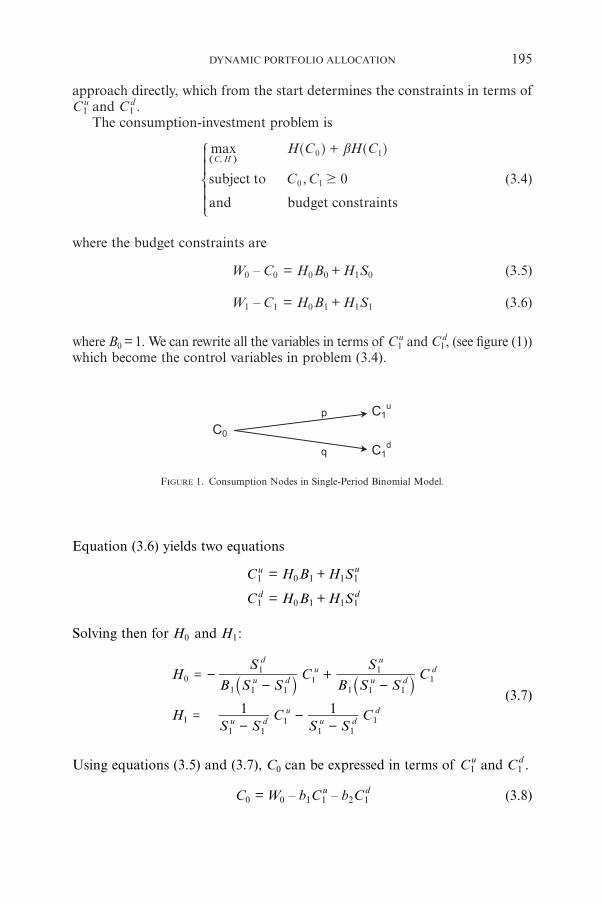
FIGURE 1. Consumption Nodes in Single-Period Binomial Model.
approach directly, which from the start determines the constraints in terms ofC u
1 and C d1 .
The consumption-investment problem is
,
max H C H C
C Csubject to
and budget constraints
b
0
,C H0 1
0 1 $
+] ^ ^g h hZ
[
\
]]
]]
(3.4)
where the budget constraints are
W0 – C0 = H0B0 + H1S0 (3.5)
W1 – C1 = H0B1 + H1S1 (3.6)
where B0 = 1. We can rewrite all the variables in terms of C u1 and C d
1, (see figure (1))which become the control variables in problem (3.4).
DYNAMIC PORTFOLIO ALLOCATION 195
Equation (3.6) yields two equations
C u1 = H0B1 + H1Su
1
C d1 = H0B1 + H1Sd
1
Solving then for H0 and H1:
HB S S
SC
B S S
SC
HS S
CS S
C1 1
u d
du
u d
ud
u du
u dd
01
11
1 1
= --
+-
=-
--
1 1
1
1 1
11
1 1 1 11
` `j j(3.7)
Using equations (3.5) and (3.7), C0 can be expressed in terms of C u1 and C d
1 .
C0 = W0 – b1C u1 – b2C d
1 (3.8)
8464-05_Astin36/1_08 29-05-2006 15:20 Pagina 195
where
bB S S
B S Su d
d
11
1 0=
-
-
1 1
1` j and bB S S
S B Su d
u
21
1 0=
-
-
1 1
1` j
Interpretation of b1 and b2:
For the choice of Sd1 < B1S0 < Su
1 , it is easy to check that Q(w1) = (B1S0 – Sd1 ) /
(Su1 – Sd
1 ) and Q(w2) = (Su1 – B1S0) / (Su
1 – Sd1 ) define a martingale measure for
the discounted price S1 /B1. Therefore
b1C u1 + b2C d
1 = B�C
Q1
1< F
And equation (3.8) can be written as
W0 = C0 + B�C
Q1
1< F
The absence of arbitrage condition is equivalent to Q(wi) ∈ (0,1) for i ∈{1,2}.Provided that B1 = (1 + r) ≥ 1, we also have bi / Q(wi) /B1 ∈ (0,1).
The problem (3.4) is then equivalent to
0
,
/
max
�
H C H C
C C
W C C r
subject to
b
0
1
,C H
Q
0 1
0 1
0 1
$
+
= + +
] ^ ^
]g h h
g6 @(3.9)
This would be the starting point if the optimal portfolio problem (3.4) was for-mulated within the risk-neutral computational approach.
The constraints of Problem (3.4) are:
(1) C u1 ≥ 0 and C d
1 ≥ 0
(2) W0 – C0 ≥ 0 ⇒ b1Cu1 + b2C
d1 ≥ 0 (using (3.8))
(3) C0 ≥ 0 ⇒ b1Cu1 + b2C
d1 ≤ W0 (using (3.8))
Solving the Problem – Feasible Region. In this section, we consider the spe-cial case when the distortion functions g and h are conjugate, and we solve theproblem analytically. The general case of non-conjugate distortion functionsis left to the next paragraph dealing with the case of 2 risky assets and 1 risk-less security.
196 M. HAMADA, M. SHERRIS AND J. VAN DER HOEK
8464-05_Astin36/1_08 29-05-2006 15:20 Pagina 196
Let us write all the variables in terms of C u1 and C d
1 :
• H(C0) = C0 = W0 – b1C u1 – b2C d
1
h(p)C u1 + [1 – h(p)]C d
1 if C u1 ≥ C d
1• H (C1) =
h(q)C d1 + [1 – h(q)]C u
1 if C u1 ≤ C d
1
Therefore, the objective function in the problem (3.9) is equal to
W0 + {bh(p) – b1}C u1 + {b (1 – h(p)) – b2}C d
1 if C u1 ≥ C d
1H (C0) + bH (C1) =
W0 + {b (1 – h(q)) – b1}C u1 + {bh (q) – b2}C d
1 if C u1 ≤ C d
1
We consider then the two maximization problems
0
,
max
P
h p b C h p b C
C C
C C
b C b C W
subject to
b b 1
0 0
,C C
1
1 2
1 2
$ $
$
#
=
- + - -
+
1 1
1 1
1 1
1 1
u d
u d
u d
u d
1 1u d
^ ^^h hhZ
[
\
]]]]
]]]]
" #, -(3.10)
and
0
,
max
P
h q b C h q b C
C C
C C
b C b C W
subject to
b b1
0 0
,C C1 2
1 2
$ $
#
#
=
- - + -
+
1 1
1 1
1 1
1 1
u d
u d
u d
u d
1 1
2
u d^^ ^hh hZ
[
\
]]]]
]]]]
# "- ,(3.11)
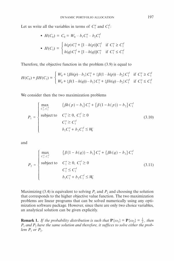
Maximizing (3.4) is equivalent to solving P1 and P2 and choosing the solutionthat corresponds to the higher objective value function. The two maximizationproblems are linear programs that can be solved numerically using any opti-mization software package. However, since there are only two choice variables,an analytical solution can be given explicitly.
Remark 1. If the probability distribution is such that P{w1} = P{w2} = 21 , then
P1 and P2 have the same solution and therefore, it suffices to solve either the prob-lem P1 or P2 .
DYNAMIC PORTFOLIO ALLOCATION 197
8464-05_Astin36/1_08 29-05-2006 15:21 Pagina 197
FIGURE 3. Solution to the Single-Period Portfolio Problem in the Dual Theory.
FIGURE 2. Feasible regions for consumption in one-period model.
198 M. HAMADA, M. SHERRIS AND J. VAN DER HOEK
8464-05_Astin36/1_08 29-05-2006 15:21 Pagina 198
Given the constraints, feasible sets of the solution to P1 and P2 are illustratedin Figure (2). Possible solutions are indicated by the little arrows.
The objective function in the problem (3.10) is linear in C u1 and C d
1 . Theequation of the line representing the level curve of the objective function at apossible value z1 is given by
Ch p b
zh p b
h p bC
b bb
1 12 2
1=- -
-- -
-1 1d u1^^ ^^ ^
hh hhh(3.12)
There are four possible solutions of the problem corresponding to the summitsof the feasible region
(0, 0), 0, bW
02
d n, 0 0,b bW
b bW
1 2 1 2+ +d n and 0 ,b
W0
1d n. (3.13)
Figure 3 plots the solution for the case where b = 0.95, r = 10% and r = 0.8.Optimal Investment Strategies. Once the optimal consumption rules are obtained,the optimal investment strategies follow from the budget equations (3.7).
• When (C u1 ,C d
1 ) = (0,0), then (H0, H1) = (0,0)
• When (C u1 ,C d
1 ) = ( 0 , 0bW
1), then (H0, H1) = ( 0 0,W W
B S S
S
B S S
B-
- -0 01
1
1d
d
d1 1
1 ).
• When (C u1 , C d
1 ) = ( 0 0,b bW
b bW
1 1+ +2 2), then (H0, H1) = (W0, 0). This situation is
referred to as “plunging”.
• When (C u1 ,C d
1 ) = ( 0,0 bW
2), then (H0, H1) = ( 0 0,W WS B S
S
S B SB
-- -0 01
1
1u
u
u1 1
1 ).
4. OPTIMAL PORTFOLIO CHOICE IN A MULTI-PERIOD MODEL
4.1. General Set-up
As discussed in Section 2.2, the consumption-investment problem is:
t. .
,
�
Max H C
s t vr
C
C t T
b
1
0 0
, ,...,C C Ctt
tt
t
Q
0
0
T0 1
6$ !
=+
=
=
T
T
t!
!
^
]h
g=6
G@
Z
[
\
]]]
]]]
(4.1)
where v is the initial wealth and r is a constant interest rate.
DYNAMIC PORTFOLIO ALLOCATION 199
8464-05_Astin36/1_08 29-05-2006 15:22 Pagina 199
Problem (4.1) is set up in the discrete-time case. However, it can be solvednumerically either with a finite number or a continuum states at each timeperiod.
Let us consider the case when at each time t, Ct takes (2t +1) possible values(recombining trinomial tree), then Ct is a vector of 2t +1 control variables, i.e.
Ct = [Ct,– t, …,Ct,0 , …, Ct, t ] ∈ �+2t +1
For each vector Ct, there exists a corresponding vector
pt = [ pt,– t, …, pt,0 , …, pt, t ] ∈ [0,1]2t +1
where pt, i = P [Ct = Ct, i ].
From Proposition (No order assumption), one way to write the term H(Ct) inthe objective function is:
H(Ct) = C .F p C ,i t
t
t t i,t i= -
! ^ h
Where the function
FCt, i: [0,1]2t +1
$ �+
pt = [ pt,– t,…, pt,0,…, pt,t ] 8(4.2)
g p g p I
h p h p I1 1
<
< >
a
a
kC C kC C C
kC C kC C C
, , , , ,
, , , , ,
t k t i t k t i t i
t k t i t k t i t i
-
+ - - -
# #
#
! !
! !
b bb b
l ll l
;;
EE
Z
[
\
]]
]]
! ! !! ! !
_
`
a
bb
bb
+ + ++ + +
Remark 2. Another formulation is also possible using Proposition (Order assump-tion), where the control variables are ordered explicitly.
The general expression (4.2) can be significantly simplified in the case when gand h are conjugate functions and the consumption at each time is distributedwith the same probability over the states, i.e.
g(x) = 1 – h(1 – x) ∀x ∈ [0,1]
and
P [Ct = Ct, i ] = qt = t2 11+
∀t ∈ [1,T ], ∀i ∈ [– t, t ]
200 M. HAMADA, M. SHERRIS AND J. VAN DER HOEK
8464-05_Astin36/1_08 29-05-2006 15:22 Pagina 200
Then, using Proposition (conjugate), we have
C # # <F p g t C C g t C C2 11
2 11
, , , ,t t k t i t k t i,t i#=
+-
+^ b bh l l# #- -
where #{Ct,k ≤ Ct, i} denotes the number of variables Ct,k, k ∈{– t,…, t}, suchthat Ct,k ≤ Ct, i .
In this case, the problem (4.1) can be solved using one of the simplicialalgorithms used in rank regression problems. Osborne (2001 [14]) is an excellentreference for solving such types of problems.
4.2. Application: Wang’s class of distortion operators
Now consider another class of distortion operators introduced by Wang (2000[22]). Wang shows that applying this distortion operator to a stock price dis-tribution, the risk neutral valuation of stock prices can be recovered in the nor-mal and the lognormal cases. Further investigations, however, should be car-ried out to check whether this statement is true for any contingent claim, andalso when there is no normality assumption on the underlying asset prices.Hamada & Sherris (2001[8]) provide some insight into this question.
4.2.1. The operator. Let X be a random variable with a decumulative distribu-tion function SX(x) = P [X > x]. The expectation of X is alternatively given by:
� X S x dx S x dx1X X
0
0= - +
3
3
-# #] ]g g6 6@ @
Let F(u) = e dxu
p21 x
2
3-
-2
# be the standard normal cumulative function and a ∈ �,
the distortion operator is defined as:
ga(u) = F[F–1(u) + a ]
for u in [0,1]. The risk-adjusted premium of X, as defined by Wang (2000) admitsthe following Choquet representation
,aH X g S x dx g S x dx1a aX X
0
0= - +
3
3
-# #] ]g g6 6 6@ @ @" ,
When X is positive, we have:
,aH X g S t dta X0
=3# ] g6 6@ @
DYNAMIC PORTFOLIO ALLOCATION 201
8464-05_Astin36/1_08 29-05-2006 15:23 Pagina 201
The risk-adjusted premium is evaluated as in Yaari’s dual theory of choice underuncertainty. The tail distribution SX (t) is distorted by the function ga(p) =F[F–1(p) + a ]. This operator shifts the pth quantile of X by a positive or neg-ative value a and reevaluates the normal cumulative probability of the shiftedquantile.
If a > 0, then ga(p) > p, if a < 0, then ga(p) < p. Since ga is continuous andga(p) ∈ [0,1], then:
ga is convex if a < 0
ga is concave if a > 0
The investor behaves pessimistically by shifting the quantiles to the left, therebyassigning high probabilities to low outcomes, and behaves optimistically byshifting the quantiles to the right thereby assigning high probabilities to highoutcomes. Typically, an insurer has a lower a than a reinsurer when pricing thesame risk.
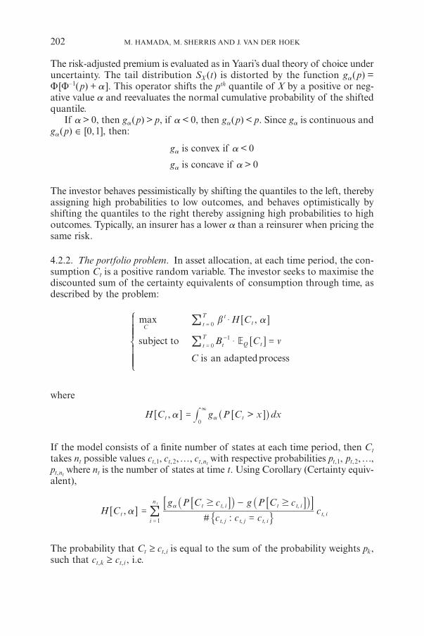
4.2.2. The portfolio problem. In asset allocation, at each time period, the con-sumption Ct is a positive random variable. The investor seeks to maximise thediscounted sum of the certainty equivalents of consumption through time, asdescribed by the problem:
,max
�
aH C
B C vsubject to
bC
ttt
T
t Q tt
T
0
1
0
$
$ =
=
-
=
C is an adaptedprocess
!
!
66
@@
Z
[
\
]]]
]]]
where
, aH C g P C x dxat t0
=3
># ^ h6 6@ @
If the model consists of a finite number of states at each time period, then Ct
takes nt possible values ct,1, ct,2,…, ct,ntwith respective probabilities pt,1, pt,2,…,
pt,ntwhere nt is the number of states at time t. Using Corollary (Certainty equiv-
alent),
c c
c cc
c,
:#aH C
g P C g P C
, , ,
, ,,
a
tt j t j t i
t t i t t i
i
n
t i1
$ $=
=
-
=
t
! _ _i i6 7 78@ A A B# -
The probability that Ct ≥ ct,i is equal to the sum of the probability weights pk,such that ct,k ≥ ct,i , i.e.
202 M. HAMADA, M. SHERRIS AND J. VAN DER HOEK
8464-05_Astin36/1_08 29-05-2006 15:24 Pagina 202
FIGURE 4. Trinomial lattice encoding.
P [Ct ≥ ct,i ] =c c
p ,:
t kk , ,t k t i$
!! +Hence,
c cc
c
c c c c,
:#aH C
g p g p
, , ,
: : >
,
a
tt j t j t i
kk kk
i
n
t i1
, , , ,t k t i t k t i=
=
-$
=
, ,t tt ! !!
b bl l6 ;@ E#
! !-
+ +
By defining the risk-neutral probability and using the expression above, thedescription of the problem is complete. This is not a linear program, howeverit can be solved using an optimisation package. The next paragraph showshow to solve it on a trinomial lattice and provides some results in two periods.
4.2.3. How to compute H [C, a ] over a lattice? Fix a time t, and consider thedistribution of the consumption represented by the vertical nodes (t, i ) – t ≤ i ≤ t .At time t, the consumption Ct takes 2t +1 possible values ct,i with probabilitiespt,i = P [S = St,i ] ; see Figure (4). Hence,
c cc
c
c c c c,
:#aH C
g p g p
, , ,
: : >
,
a a
tt j t j t i
kk kk
i
t
t i, , , ,t k t i t k t i
==
-$
= - t
, ,t t! !!
b bl l6 ;@ E#
! !-
+ +
DYNAMIC PORTFOLIO ALLOCATION 203
8464-05_Astin36/1_08 29-05-2006 15:25 Pagina 203
The probabilities pt,i , t ∈{1,…,T}, i ∈{–t,…,0,…,t} can be specified as follows:
p P S S
tk
t kk i p p p p1
, ,
( , )max
t i t i
uk
dk i
u dt k i
i k t i
2
02
$ $ $
= =
=--
- -# #
- - +
+
! c d ^m n h7
7
A
A(4.4)
where pu and pd are respectively the probabilities of up and down jumps and[x] is the integer part of x. The expression (4.4) is a generalisation of the prob-abilities in a binomial model. Likewise, the expression �Q [Ct ] in the constraintscan be computed. In effect,
�Q [Ct ] = Q c, ,t i t ii t
t
$= -
!
where:
Q Q S S
tk
t kk i q q q q1
,
( , )max
t i
uk k i
u dt k i
i k t i
2
02
$ $ $
= =
=--
- -# #
- - +
+d
,t i
! c d ^m n h7
7
A
Awhere qu and qd are respectively the risk-neutral probabilities of up and downjumps.
5. NUMERICAL RESULTS
This section provides two numerical examples of portfolio allocation using theclasses of distortion operators introduced earlier.
The first example considers Wang’s distortion operator. Suppose that thereare three dates t = 0,1,2 and five states of the world. This corresponds to arecombining trinomial lattice. We numerically solve the problem (4.3) for T = 2.For a loading parameter a = 0.5, Figure (5) shows the consumption and invest-ment strategies as well as the wealth process for a two period example. The dis-count factor b = 0.9, the risk-free interest rate r = 10% and initial wealth v = $10.
The jump probabilities are pu = pm = pd = 31 and qu = 15
2 , qm = 31 and qd = 15
8 .For this choice of risk neutral probabilities, and a correlation coefficient r = 0.75,the means and volatilities of the two risky securities are respectively: mean1 =13.46%, volatility1 = 07.07%, and mean2 = 15.20%, volatility2 = 10.61%.
The intermediate consumption C is null and the consumption is strictlypositive at the highest state of the world. However, intermediate positions nr,r1 and r2 in the riskless asset, the first security and the second security respec-tively are nonzero.
204 M. HAMADA, M. SHERRIS AND J. VAN DER HOEK
8464-05_Astin36/1_08 29-05-2006 15:25 Pagina 204
FIGURE 5. Consumption and investment strategies using Wang’s distortion operator.
To see the impact of the loading parameter a on the consumption stream,Figure (6) plots the optimal consumption for different values of a .
Around the value a = – 0.8, there is a switch in consumption from the low-est state, where it is nonzero and null elsewhere, to the highest state.
A closer look at the consumption process around a = – 0.8, is representedin Figure (7). This figure shows that in the transitory passage across the levela = 0.8, the intermediate consumption becomes nonzero.
From the examples above, it is clear that the linearity of the dual utility inconsumption results in a corner solution in the optimisation problem. This isnot a desirable feature in portfolio selection, although, as shown in the example,with 3 assets, diversification is possible. On the other hand, within the expectedutility framework, a risk averse investor is always diversifying provided that theexpected return of the risky asset is positive.
DYNAMIC PORTFOLIO ALLOCATION 205
8464-05_Astin36/1_08 29-05-2006 15:25 Pagina 205
FIGURE 6. Consumption process as function of the loading parameter a.
FIGURE 7. Consumption process as function of the loading parameter a (a zoom into – 0.8)
206 M. HAMADA, M. SHERRIS AND J. VAN DER HOEK
8464-05_Astin36/1_08 29-05-2006 15:25 Pagina 206
FIGURE 8. Optimal consumption and trading strategies using PH risk measure.
The second example is a numerical solution to the problem (??) where therisk measure is the one introduced by van der Hoek and Sherris. Figure (8)shows the optimal consumption and trading strategies for the parameters valuesindicated in the figure.
This numerical example shows that consumption at the end of the investmentperiod is positive in all the states. This is due to the asymmetry resulting frompricing the downside of the risk using the distortion function g(x) = x0.2 andthe upside of the risk using h(x) = 1 – (1 – x)0.9. It is worth noting that the con-sumption in the middle and the down state equals the benchmark consumptiona = 5. This is consequence of the linearity in Problem (??) where C = a is a cor-ner solution.
6. CONCLUSION
In this paper we have provided a formal treatment of risk measures based ondistortion functions in discrete-time setting. We have also shown that the riskneutral computational approach is well adapted to portfolio optimisation withsuch measures that don’t lie within the expected utility framework.
The application to two different distortion operators shows that the portfo-lio consumption and investment rules are different from the expected utility resultssince the optimisation leads to corner solutions resulting from the linearity of
DYNAMIC PORTFOLIO ALLOCATION 207
8464-05_Astin36/1_08 29-05-2006 15:25 Pagina 207
the objective in the control variables. This is an undesirable feature and animportant area that needs to be addressed before these non-expected utility riskmeasures can be confidently applied to asset allocation. This is an area forfuture research. One possibility is to consider combining expected and non-expected utility measures as in Quiggin (1982 [15]).
REFERENCES
[1] ALLAIS, M. (1953) Le comportement de l’homme rationnel devant le risque. Economertica,21, 503-546.
[2] BUFMAN, G. and LEIDERMAN, L. (1990) Consumption and asset returns under non-expectedutility, some new evidence. Economics letters, 34, 231-235.
[3] CAMERER, C.F. (1989) An experimental test of several generalized utility theories. Journalof Risk and Uncertainty, 2(1), 61-104.
[4] EPSTEIN, L.G. and ZIN, S.E. (1989) Substitution, risk aversion, and the temporal behaviorof consumption and asset returns: An empirical analysis. Carnegie-Mellon University, Pit-tersburg, PA.
[5] EPSTEIN, L.G. and ZIN, S.E. (1989) Substitution, risk aversion, and the temporal behaviorof consumption and asset returns: A theoretical framework. Econometrica, 57(4), 937-69.
[6] FISHBURN, P.C. (1988) Nonlinear preference and utility theory. Johns Hopkins Series in theMathematical Sciences, no 5. Baltimore and London, pp. xiv, 259.
[7] GIOVANNINI, A. and JORION, P. (1989) Time-series tests of a non-expected utility model ofasset pricing. Columbia University, New York.
[8] HAMADA, M. and SHERRIS, M. (2001) On the relationship between risk neutral valuationand pricing using distortion operators. Working paper.
[9] HE, H. (1990) Convergence from discrete to continuous-time contingent claims prices. TheReview of Financial Studies, 3(4), 523-546.
[11] KAHNEMAN, D. and TVERSKY, A. (1979) Prospect theory: An analysis of decision under risk.Econometrica, 47, 263-291.
[12] KOSKIEVIC, J.-M. (1999) An intertemporal consumption-leisure model with non-expectedutility. Economics Letters, 64, 285-289.
[13] KREPS, D.M. and PORTEUS, E.L. (1978) Temporal resolution of uncertainty and dynamicchoice theory. Econometrica, 46(1), 185-200.
[14] OSBORNE, M. (2001) “Simplicial Algorithms for Minimizing Polyhedral Functions”. Cam-bridge University Press.
[15] QUIGGIN, J. (1982) A theory of anticipated utility. Journal of Economic Behavior and Orga-nization, 3, 323-343.
[16] ROEL, A. (1985) Risk aversion in quiggin and yaari’s rank-order model of choice underuncertainty. The Economic Journal.
[17] ROSS, S.A. (1981) Some stronger measures of risk aversion in the small and in the largewith aplications. Econometrica, 49, 621-638.
[18] VAN DER HOEK, J. and SHERRIS, M. (2001) A class of non-expected utility risk measuresand implications for asset allocations. Insurance: Mathematics and Economics 28, 69-82.
[19] WANG, S. (1996) Ambiguity aversion and the economics of insurance. University of Water-loo, research report 96-04.
[20] WANG, S. (1996) Premium calculation by transforming the layer premium density. AstinBulletin, 26, 71-92.
[21] WANG, S. (1998) Implementation of proportional hazards transforms in ratemaking. Pro-ceedings of the Casualty Actuarial Society LXXXV. Available for download on http://www.casact.org/pubs/proceed/proceed98/index.htm.
[22] WANG, S.S. (2000) A class of distortion operators for pricing financial and insurance risks.The Journal of Risk and Insurance, 36(1), 15-36.
208 M. HAMADA, M. SHERRIS AND J. VAN DER HOEK
8464-05_Astin36/1_08 29-05-2006 15:25 Pagina 208
[23] YAARI, M.E. (1986) “Univariate and Multivariate Comparison of Risk Aversion: A NewApproach”. Cambridge University Press.
[24] YAARI, M.E. (1987) The dual theory of choice under risk. Econometrica, 55, 95-115.
MAHMOUD HAMADA
School of Finance and EconomicsUniversity of Technology of SydneySydney, AustraliaE-mail: [email protected]
APPENDIX A.
PROPERTIES OF THE CERTAINTY EQUIVALENT IN DUAL THEORY
A.1. General Case
Let g be a continuous, non-decreasing function, g : [0,1] → [0,1] with g(0) = 0and g(1) = 1, and X be a positive random variable representing a risk. The riskX is measured by its certainty equivalent defined as:
X g S t dtP X0
=3#] ]^g gh
In the discrete-time case, X takes n possible values (X(w1), X(w2), …, X(wn))with probabilities (p1, p2,…, pn), where n ∈ � \{0}. In probabilistic notation, letW = {w1, w2,…, wn} be the probability space where wi , i ∈ {1,…,n} are the statesof the world, then P [wi] = pi ∀i ∈ {1,…,n}.
This is typically the case of a tree model, where the number of states growsas time evolves. The following theorem gives an expression of P(X) in the dis-crete case.
Theorem 1 (Certainty equivalent). If X is a random variable taking on n distinctvalues X(w1),X(w2),…,X(wn) with respective probabilities p1, p2, …, pn then,
P(X) = �̂g [X ]
where �̂g [X ] is a weighted average of possible values of X, such that the weightPg(wi) assigned to X(wi) is given by:
�̂g [X ] can be interpreted as an expectation where the probability assigned toa possible value of X depends also on the other values.
DYNAMIC PORTFOLIO ALLOCATION 209
8464-05_Astin36/1_08 29-05-2006 15:25 Pagina 209
Proof. To simplify notation, let xi = X(wi), i ∈ {1,…,n}. If we denote x(i) theith value in increasing order (order statistics), then we have:
>
>
>
>
.... ....
>
Pr X t
x t
p x t x
p x t x
p x t x
t x
if
if
if
if
if
1
0
( )
( ) ( )
( ) ( )
( ) ( )
( )
kk
n
kk
n
n n n
n
1
2 12
3 23
1
$
$
$
$
=
=
=
-
!!6 @
Z
[
\
]]]]]
]]]]]
Therefore,
( ) ...X g dt g p dt g p dt g p dt
x g x x
g g x
P 1
( )
kk
n
x
xx
kk
n
x
x
nx
x
ip
i ii
n
ip
ip
i
n
i
20 3
1 11
1
11
( )
( )( )
( )
( )
n
n
1
21
2
3
1
$
= + + + +
= + -
= -
= =
+=
-
-=
-
## # #! !
!
!
] e e ^]]
] ]
]
g o o hgg
g g
g
88
BB
where
>
g g p
g P X x
i kk i
n
i
1
=
=
= +
p !e]`
og j8 B
210 M. HAMADA, M. SHERRIS AND J. VAN DER HOEK
Since g is an increasing function from [0,1] to [0,1], and ∀i >p pk kk i
n
k i
n
1= +=!!
then:
for all i in {1..n}, Pgi / g p g pk
k i
n
kk i
n
1
-= = +
! !e eo o ∈ [0,1]
Moreover, .P g p g g0 1 1i kk1 1
= - = == =i
n ng! !` ] ]j g g Therefore {Pg1 , Pg
2 , …, Pgn }
define a probability measure on the probability space W = {w1, w2,…, wn}. ¡
This theorem states that in the discrete-time case, the certainty equivalent of X isequivalent to an expectation under another probability measure. This has beenshown when all the possible values of X are distinct. The question that arisesimmediately is: what happens in the case when some possible values of X coin-cide? The following example provides an insight into this question.
8464-05_Astin36/1_08 29-05-2006 15:27 Pagina 210
In the general case when some values of X coincide, order them in increasingorder, then from each set of equal values keep only one value and assign theprobability of the set to this value. Thus, a new variable Y is defined in such away that all the elements of Y are strictly increasing with adjusted probabilityweights such that the identity P(X ) = P(Y ) is satisfied.
Another approach consists of keeping the redundant values and dividingthe probability weights by the number of these values. This is the idea of thenext corollary:
Corollary 1. If X is a random variable taking n possible values X(w1), X(w2),…,X(wn) with probabilities (p1, p2, …, pn), then,
P(X ) = �̂g [X ]
where �̂g [X ] is a weighted average of possible values of X, such that the weight Pg
assigned to X (wi) is given by:
j j:
>
# X X X
g P X X g P X Xw
w
w wP
$=
=
-
w wii
i ig^ _ _ ^^_ ^_h i i h
h i h i6 6@ @# - for all wi in W
where the notation #{X(wj) : X(wj) = X(wi)} stands for the number of values X(wj)equal to X(wi).
Proof. The idea of the proof is given in the previous example. In formal terms,let
Define a new random variable Y and a subset of indices S ⊆ {1,…,n}, such that:
DYNAMIC PORTFOLIO ALLOCATION 211
8464-05_Astin36/1_08 29-05-2006 15:27 Pagina 211
Y (wi) = X (wi) ∀i ∈ S
Y (wi) ! Y (wj) for i ! j, ∀(i, j ) ∈ S2
Image(Y ) = Image (X )
where Image(X ) is the set of all possible values taken by X.
By applying the theorem to Y whose values are all distinct, we have:
s
j j:#
Y P Y
P X
P X
X X XP X
w w
w w
w w
ww w
P
1
ss S
s
s
s s s
s S
ss S i
i
n
C
1
=
=
==
!
!
! !
= w w i
CC
C
g
g
g
g
i i
i i
!
!
! !
!
] ^ ^^ ^
^ ^
_ _ ^^ ^
g h hh h
h h
i i hh h
# -
Since
Pr[X > t ] = Pr[Y > t ] ∀t ≥ 0
then,
P (Y ) = P (X )¡
A.2. Application: Van der Hoek and Sherris class of risk measures
Corollary 2 (Position of a). If X is a multinomial discrete random variable takingthe values (x1, x2, …, xn) such that x1 < x2 < … < xn, with probabilities (p1, p2, …,pn), then,
• If a ≤ x1, then:
H X x h x x
h h x
ip
i
n
i i
ip
ip
i
n
i
1
1
1
11
= + -
= -
=
-
+
-=
1 !
!
] g 68
@B
212 M. HAMADA, M. SHERRIS AND J. VAN DER HOEK
8464-05_Astin36/1_08 29-05-2006 15:28 Pagina 212
• If a ≥ xn, then:
H X x g x x
g g x
n ii
n
i i
i ii
n
i
1
1
1
11
= + -
= -
=
-
+
-=
p
p p
!
!
] g 68
@B
• If a ∈ [xr , xr +1) where r ∈ {1,…, n – 1}, then:
g aH X h g g x h h x1 rp
i ii
r
i i ii r
n
i11
11
= - - + - + --=
-= +
p p p prp ! !] g 8 8 8B B B
where
h h p1 kk
i
1
= -=
ip !e o and g g pk
k
i
1
==
ip !e o
This corollary illustrates the idea of pricing the upside and the downside ofthe risk differently. In effect, for outcomes xi’s below the level a, the proba-bility distribution is distorted by the function g, and for outcomes xi’s abovethe level a, the probability distribution is distorted by the function h.This is a flexible way to price risk around some benchmark a. The choice ofthe distortion functions g and h reflects the risk behaviour of the investor.Indeed, h is convex, then 2h(x) ≤ h(x – 1) + h(x + 1) wherever h is defined.Therefore
<h p h p h p h p1 1 1 1kk
i
kk
i
kk
i
kk
i
1
1
1 1
2
1
1
- - - - - -=
-
= =
-
=
-
! ! ! !e e e eo o o o
or
hpi – 1 – hp
i < hpi – 2 – hp
i – 1
So the probability assigned to the outcome xi is less than the probabilityassigned to xi – 1. In other terms, the investor assigns lower probabilities tohigher outcomes. The more risk averse the investor, the more convex the dis-tortion function h. The same argument applies to the concavity of g.
Furthermore, the choice of h with respect to g reflects how the investorconsiders the risk with respect to the benchmark a. For some choice of gand h, pricing risk does not depend on a. This is the idea of the followingproposition:
DYNAMIC PORTFOLIO ALLOCATION 213
8464-05_Astin36/1_08 29-05-2006 15:28 Pagina 213
Proposition 2 (Conjugate). Let X be a random variable taking on n distinct valuesX(w1), X(w2),…,X(wn) with probabilities p1, p2, …, pn. In the case when h and gare conjugate, we have
H (X) = �̂h [X ] (A.1)
where the weighted average weights are given by
Ph(w) = h (P [X ≥ X (w)] ) – h (P [X > X (w)] ) ∀w ∈ W (A.2)
Proof. In the case when h and g are conjugate, i.e., h(1 – x) = 1 – g(x), in Appen-dix 2, we show that:
H (X ) = H0,0,h(X ) = h0
3# (P [X > t ] ) dt
Therefore, the proposition follows from Theorem (Certainty equivalent). ¡
Proposition 3 (No order assumption). For a multinomial discrete random vari-able X taking the values (x1, x2, …, xn), with probabilities (p1, p2, …, pn), xi ! xj
if i ! j then,
H (X ) = Const + x xg I h I x, ,>a a
p Xip X
i
n
1i i
+#=
i i! ` j! !+ +where
x x
x x
x x
a
g g p g p
h h p h p
Const h p g p
1 1
1 1
,
<
,
<
a a
p Xk
xk
x
p Xk
xk
x
k k
k k
k k
k k
= -
= - - -
= - - -
#
#
# #
i
i
i i
i i
! !
! !
! !
J
LKK
J
LKK
J
LKK
J
LKK
J
LKK
J
LKK
N
POO
N
POO
N
POO
N
POO
N
POO
N
POO
R
T
SSS
R
T
SSS
V
X
WWWV
X
WWW
! !
! !
! !
+ +
+ +
+ +
and the notation
xxp p I
aak k
k
n
1k
k=
##
=
! !! !+ +
where x ak #I! + is the indicator function on the set {xk ≤ a}.
214 M. HAMADA, M. SHERRIS AND J. VAN DER HOEK
8464-05_Astin36/1_08 29-05-2006 15:29 Pagina 214
APPENDIX B.PROOF OF PROPOSITION (ORDER ASSUMPTION)
Proof. For x1 < x2 < … < xn we have:
(x1 – a)+ ≤ (x2 – a)+ ≤ … ≤ (xn – a)+ and (a – x1)+ ≥ (a – x2)