FILE 02282-1- THE UNiVERSITYf OF MICHIGAN COLLEGE OF ENGINEERING DEPARTMENT OF ELECTRICAL ENGINEERING & COMPUTER SCIENCE - Radiation Laboratory --- *IMILLIMETER WAVE RADAR CLUTTER PROGRAM Fawwaz T. Ulaby Radiation Laboratoev Department of Electical Engineering .* and Computer Science ~1' The Unviersity of Michigan Ann Arbor, MI 48109-2122 "IR1 FINAL REPORT D TILCE * . . U.S. Army Research OfficeNO2 Box 12211 ..- Research Triangle Park, NC 27709- Contract DAAG29-85-K-0220 .- :"October, 1989 ... .. -.. ,,APPROVED FOR PULCREESDISTRII3UTi*ON -.. UNLIMITED ... 4 89 102 0
Transcript
FILE 02282-1-
THE UNiVERSITYf OF MICHIGANCOLLEGE OF ENGINEERINGDEPARTMENT OF ELECTRICAL ENGINEERING & COMPUTER SCIENCE
- Radiation Laboratory ---
*IMILLIMETER WAVE RADAR CLUTTER PROGRAM
Fawwaz T. UlabyRadiation LaboratoevDepartment of Electical Engineering .*
and Computer Science~1' The Unviersity of Michigan
Ann Arbor, MI 48109-2122
"IR1 FINAL REPORT D TILCE* .. U.S. Army Research OfficeNO2
Box 12211 ..-
Research Triangle Park, NC 27709-
Contract DAAG29-85-K-0220 .-
:"October, 1989 ... ..
-..,,APPROVED FOR PULCREESDISTRII3UTi*ON-.. UNLIMITED ... 4
89 102 0
DISCLAIMER NOTICE
THIS DOCUMENT IS BEST
QUALITY AVAILABLE. THE COPY
FURNISHED TO DTIC CONTAINED
A SIGNIFICANT NUMBER OF
PAGES WHICH DO NOT
REPRODUCE LEGIBLY.
PE ST VAILAIS-L
MILLIMETER WAVE RADAR CLUTTER PROGRAM
Aos0s16 For
NTIS GRA& I
FINAL REPORT DTIC rAU.S. ARMY RESEARCH OFFICE Ummo= 0CONTRACT DAAG29-85-K-0220 Just'float Ion
Avalebility Codes
Dist SpeelaJ
t-/iFawwaz T. Ulaby
Radiation LaboratoryElectrical Engineering and Computer Science
University of MichirjanAnn Arbor, Michigar' 48109
October, 1939
THE VIEW, OPIN!ONS, AND/OR FINDINGS CONTAINEDIN THIS REPORT ARE THOSE OF THE AUTHOR(S) ANDSHOULD NOT BE CONSTRUED AS AN OFFICIALDEPARTMENT OF THE ARMY POSITION, POLICY, ORDECISION, UNLESS SO DESIGNATED BY OTHERDOCUMENTATION.
UNCLASSIFIED MASTER COPY -FOR REPRODUCTION PURPOSES51CUlrIy CLASSIFIC.ATlCN OF flWtS PAGE
Za.SEURTYCLAnTot4 AUTWORITY 3. 0ISTRi1WTiui VAILAjIUTY Of RMPRT
2b. DEC ASSIiCATION/0OW -4AOING SC141. Approved f or public release;distribution unlimited.
4. PERMIRMING OIRGMdiZATIOIN REPORT NUM4E(S S. MONITORING ORGANIZATION REPORT NUMIER(S)
Go. NAMf OF PfcoRmIN OnrAmaATIom I& oBb. OFIESYMBL 7&. NAMEI Of MONITORING ORGANiZATIONRadiation Laboratrcry, University I(wf ̂ W*cabkiof Michig~an, Ann Arbor, MI 43109 J_______ U. S. a~zjResearch Office
kr ADDRESS (OtM Sta". AnN WC) 7b. ADDRESS (0)l. State, anZI W
Ann Arbor, Michigan 48109 P. 0. Box 12211Research Triangle Park, NC 27709-22111
I&. NAME OF FUNOEING/SPVSOt4G w lb. ~ O ~SMumL 9. PROC'iJL.4EN"T iNSTNUMENT ICISTV4CATION NUMBERORGAJ4IZATION ^ P9-k-oaf.o
U. S. Army Research Office N (A__ 6__ 11-__?';-___k- _____2-2-___
ReerhTriangle Park, NC 27709-2211 ELMN No Eo.N.CCESSION P40.
i1. TITLE (kxkqu Secw~ily cGin.Vca~on
Millimeter Wave Racar Clutter Program
12. PERSONAL. AJTHORMS
Pawwaz T. Ulabv13. YP O RPOT 11b TIECV1D14. DATE 00 REPORT ftw Ah,~a DW SPG y
13a TYI FRO REOTb. 1E018SR '?.LB.. 1 989, October 30 t' 204CON16. SUPPLEMENTARY NoTATION The view, epiniais arior findings contained in this report are those
of he authqr( ),nd shl ot becnt d as aq qicial D a~rtzent of the Ar-,y posit ion,IT7 COSATI C00OES IS SUajECT TEPJ Kxida 'm ,mn El msuteuy -i mdwwl by 1,1R c flhamborl
19. ASSTIRACT (C91:1w an Mvewm of Aw~wy and WWW by 600 malndm
See Reverse side
20. DISTRIOUTION IAVARL4M5.TY Of ABSTRACT 21. A"STRACT SECURITY C.ASSOFICAT10111
C3 0 AM AS RPT. DC3 cullon Unclassified22s. PNAME OF 11ESFO~Niga~ 1iN4VDUAI. 220. TELEPHON1 IkAitArM CW*) I UL OFfICE SYMBGOL
00 FORM 1473.a &mAm U APR **Caon may& be used %Wt1i OVRWt~utd. SIQ.. 7 L, 5AnqlO# T-os F_Allawr td~bo webok UNCLASSIFIED
UICLASSIFIEDaeCUmyy CI6A aPICAIl OP rNIS PA49
ABSTRACT
This final report provides a summary of 16N results realized from the researchactivities conducted under the sponsorship of U.S. Army Research 0 ce Contract
DAAG29-85-K-0220, entitled Millimeter Wave Radar Clutter Program". Me
overall goal of the progam was to conduct experimental measurments and
develop theoretical models to Improve our understanding of electromagnetic
wave interaction with terrain at millimeter wavelengths. The work was divided
into five major tas.ks. Ta.k= 1 involved the construction of calibrated
scatterometer systems at 35, 94, and 140 GHz. In designing, constructing, and
testing these systems, a great dra' -a 1,.,, t about system-design trade-ofts and
system stability requirements, Mnd now caIbra,..- 4ahn-,ii's were developed.
The scatterometer systems wen 'hen used In Support cf the rer..anlng to- - The
objective of Task 2 was to evaluate tt., of sjg fna, --I on the radar
backscatter from terrain. Based on experiments CO0 cted from aspr.. d
snow-covered surfaces, it was determined tha: !he Rayteig,, . -&Ang model is
applicable at millimeter wavelengths, and a model was developed .,.
frequency averaging can be used to reduce signal fading fluctuations. Task 3
involved the development cf a model that relates the tranamlsslon loss of dry
snow to crystal size in the 18-90 GHz region. In Task 4, we examined ,he
character of bistatic scattering from surfaces of various surface roughness and
from two types c1 trees. The bisttic data for trees proved Instrumental in the
development of a radar model for scattering from tre foliage at millimeter
wzve;engths, which was one component of Task 5. The other componant of Task
5 Involved the deve!opment of a model for snow.
UTICLASSIFIV.
ncumdr'v cLAi.4 ricA 1iow o m Ns PAGE
TABLE OF CONTENTS
A B S T R A C T .................................................................................................
2. SUMMARY OF RESULTS ........................................................................................ 3
2.1 Construction of millimeter-wave scatterometer ......................................... 3
2.2 Examination of radar signal statistics ........................................................... 3
2.3 Modeling extinction loss of dry snow ........................................................... 5
2.4 Examination of bistatic scattering from surfacesand volumes ........................................................................................ 6
2.5 Development of radar scattering models for terrain .................................. 7
3. LIST OF PUBLiCATIONS .............................................................................................. a
A P P E N D IX A .................................................................................................................. A .1
(1] F.T. Ulaby, T.F. Haddock, J.R. East AND M.W. Whitt. AMillimeterwave Network Analyzer based Scatterometer. IEEE
Transactions on Geoscience and Remote Sensing, Vol. 26(1). Jan.1988 ................................................................................................................... A .3
[21 M.W. Whitt and F.T. Ulaby. Millimeter-Wave PolanmetncMeasurements of Artificial and Natural Targets. IEEE Transactionson Geoscience and Remote Sensing, Vol. 26(5). Sept.1988 .................................................................................................................. A .10
[3] T.F. Haddock and F.T. Ulaby. 140-GHz Scatterorneter System andMeasuroments of Terrain. submitted for publication in IEEETransactions on Geoscience and Remote Sensing ................................ A.22
[4] M.W. Whitt and F.T. Ulaby. Milimeter-wave PolanmetricMeasurements of Artificial and Natural Targets. Proceedings ofIGARSS '87 Symposium, Ann Arbor, May 1987 ...................................... A 45
[5] F.T. Ulaby, T.F. Haddock and R.T. Austin. Fluctuation Statisticsof Millimetar-Wave Scattering from Distributed Targets.
IEEE Transactions on Geoscience and Remote Sensing, Vol.26(3), M ay 1988 ........................................................................................ A .52
[6] M.T. Haflikainan, F.T. Ulaby and T.E. Van Deventer. ExTinctionBehavior of Dry Snow in the 18- to 00- ("Hz Range. IEEETransactions on Geoscience and Remot' Sensing, VcI. GE-25(6).N ov . 198 7 .......................................................... .............................................. A .66
(71 M.T. Hailikainen, F.T. Ulaby and T.E. Van Deventer. ExtinctionCoefficient of Dry Snow at Microwave and MillimeterwaveFrequencies. Proceedings of IGARSS '87 Symposium, Ann Arbor.M ay 198 7 .......................................................................................................... A .75
(8] T.E. Van Devener, J.R. East and F.T. Ulaby. MillimeterTransmission Properties of Foliage. Proceedings of IGARSS '87,Ann Arbor. M ay 1987 .............................................................................. A.81
(91 F.T. Ulaby, T.E. Van Deventer. J.R. East. T.F. Haddock and M.E.Coluzzi. Millimeter-wave Bistatic Scattering From Ground andVegetation Targets. IEEE Transactions on Geoscience andRemote Sensing, Vol. 26(3). May 1988 ............................................... A.88
(10] F.T. Ulaby, T.F. Haddock and M.E. Coluzzi. Millimeter-waveBistatic Radar Measurements of Sand and Gravel. Proceedings ofIGARSS '87 Symposium, Ann Arbor. May 1987 ............... A.103
(11] K. Sarabandi, F.T. Ulaby, and T.B.A. Senior. Millimeter WaveScattering Model for a Leaf. Accepted for publication in RadioS cie nce .......................................................................................................... A .109
[12] F.T. Ulaby, T.H. Haddock and Y. Kuga. Measurement andModeling of Millimeter-wave Scattenng from Tree Foliage.Submitted for publication in Radio Science ................... A. 126
[131 Y. Kuga, R.T. Austin, T.F. Haddock and F.T. Ulaby. Millimeter-wave Radar Scattering from Snow Part I--Radiative Transfer Modelwith Ouasi-Crystalline Approximation. To be submitted forpublication in IEEE Transactions on Geoscicnce and RemoteS e nsing ......................................................................................................... A .162
1. INTRODUCTION
The "Millimeter Wave Radar Clutter Program" was funded by the US.
Army Research Office in September, 1985 to answer a number of important
questions related to millimeter-wave radar scattering from terrain. This Final
Report provides a summary of the research conducted and the major results
realized under this program. The program was organized in terms of the
following five tasks.
Task 1 - Contruction of Millimeter-wave
scatterometers: In order to develop valid models for radar scattering
from terrain, it .Yas imperative that we conduct careful measurements of
various types of terrain under a variety of conditions. The experimental data
servos to guide the development of the models as well as to verify their
applicability. Hence, the first task of the program focused on the
development of calibrated scatterometers with operating frequencies of 35,
94, and 140 GHz, which correspond to atmospheric-window frequencies.
Under a sepearte DOD-equipment grant, we also developed a system at
215 GHz.
Task 2 - Examination of Radar Signal Statistics: The
literature contains several models for characterizing signal fading statistics
of radar scatter from terrain. This task seeks to determine the nature of
signal fading at millimeter wavelengths and to evaluate the relationship
between the fading standard deviation and frequency bandwidth when
frequncy averaging is used.
Task 3 - Modeling Extinction Loss of Dry Snow:
Because snow is a dense medium and because the ice crystals are
comparabie to !he wavelength in size in the millimeter-wavelergth region,
the models used at the lower microwave frequencies are inapplicable at
millimeter wavelengths. The goal of this task is to develop a model for the
extinction loss of dry snow and to verify its behavior with experimental
measurement.
Task 4 - Examination of Bistatic Scattering from
Surfaces and Volumes: Prior to this program, no millimeter-wave
bistatic measurments of terrain had been reported in the literature. The
purpose of this task is to examine the character of bistatic scattering and to
use it in the development of radar scattering models. Even fcr monostatic
radar, the backscattering return includes multiple-scattering contributions that
are governed hy bistatic scattering in the medium under observation.
Task 5 - Development of Radar Scattering Models for
Terrain: Under this program, we concentrated on two types of terrain,
snow-covered ground and tree foliage. The goal of this task is to develop
electromagnetic models that can adequately describe millimeter-wave
backscatter in terms of the physical properties of the medium.
Over tha four-year duration of this program, numerous papers were
published in the literature and several presentations were made at
scientific symposia documenting the various results realized in support of
the above five tasks. A subset comprised of the major papers gonerated
under this program is included in Appendix A, and numbered 1 through 13.
2
In the next section, we shall focus on the major conclusions learnt from the
research conducted under this program without going into the details of the
experiments and models. We will refer the reader to the details by
referencing the appropriate papers in Appendix A.
2. SUMMARY OF RESULTS
2.1 Task 1 - Construction of Millimeter-Wave Scatterometers
The basic approach used in designing the millimeter-wave
scatterometers is described in paper [1]. The initial plan was to dosign and
build three systems to operate at the atmospheric-windows frequencies of
35, 94, and 140 GHz. In 1989 we added a fourth channel at 215 GHz with
funds provided by a DOD equipment grant. The salient features of the
millimeter-wave system are given in Table 1. Examples of polanmetric
measurements made at 35 GHz are given in paper [2], and example of
observations made at 140 GHz are given in paper [3].
2.2 Examinadon of Radar Signal Statistics
Based on extensive radar measurements that were conducted for
asphalt and snow-covered surfaces (see paper [5], the following results
were obtained:
(1) The Rayleigh fading model prv;des excel!ent agreement with
measurements for statistically homogeneous targets. The major cause
responsible for the confjsion that exists in the Iterature with regard to the
question of which probability density function is appropriate for
3
Table 1. Parameters of the University of MichiganMillimeter Wave Polarimeter
FREQUENCIES: 35, 94, 140, 215 GHz
IF BANDWIDTH: 0 to 2.0 GHz
SWEEP RATE: I ms/freq., 51, 101, 201, 401 freq./sweep
POLARIZATION: HH, HV, VV, VH
INCIDENCE ANGLES: 0 to 70 degrees
PLATFORM HEIGHT: 3 meters minimum, to 18 meters maximum
characterizing the statistical variability of the radar return from terrain is the
fact that the data aquirod with airborne programs includes two sources of
variability, namely that di ,e to fading and that due to the statistical in-
homogeneity of the target scene. If we study these two types of variations
seperately, we can easily compute the distribution, for the combination.
(2) Examination of the standard deviation associated with the
backscatter when frequency averaging over P bandwidth B is used,
compared to the standard deviation when no frequency averaging is used
(CW oper3tion), led to the development of a model that shows th, reduction
in signal fluctuation with bandwidth. The model is in excellent agreement
with experimental observations. The equivalent number of independent
samplo- realized by frequency averaging is approximately
N =Z-C
where D is the range resolution of the systAm and c is the velocity of light.
2.3 Task 3 - Modeling Extinction Loss of Cry Snow
A millimeter-wave model for the transmission loss of dry snow was
developed taking into account both coherent loss due to scattering and
absorption and multiple scattering effects [6, 71. The model was compared
with measurements made as a function of s:ab 2I:'ckness for 18 different
types of snow with crystal sizes varying from 0.2 mm to 2.0 mM. The
m3asurements were made at 18, 35, 60, and 90 GHz. The results foan the
basis for modeling the backscatter from snow using the radiative transfer
5
approach because prior to this investigation it was not clear as to how to
define crystal size in snow.
2.4 Task 4 - Examination of Bistatic Scattering from Surfaces
and Volumes
Papers [8] - (10] describe experiments conducted and models
developed to characterize mi:r meter-wave bistatic scatterirg from surfaces
of varyirg surface roughress ard from two distinctly different types 3f trees.
The major findirgs were:
(1) For a smooth sand surface with rms height of less than 0.1 mm,
bistatic scattering in the specular direction was found to be within a fraction
of 1dB of theory for botn horizcntal and vertical polarizations. As the
surface roughness was inzreased, the coherent specular component
decreased and diffuse scattering increased. By making measurements as a
function of both the azimuth angle and the elevation angle of the receiver,
three dimensional scatte-ing plots were generated for each polarization
configuration.
(2) Bistatic scattenng by trees can be modeled as the sum of a forward
scattering narrow-lobed Gaussian function with a beamwidth on the order of
100 and an isotropic cor, i1 onent, typically 20 dB lower in level than the peak
of the forward pattern. Inspite of the complicated geometry of the tree
architecture, insignificart differences were observed between the scattering
patterns corresponding to horizontal and vertical polarizations. This result
led to sigrificant simplifications in the c(,nstruction of a phase function for
modeling multiple scattering effects in vegetation canopies.
6
2.5 Task 5 - Development of Radar Scattering Models for
Terrain
Radiative transfer models were devefoped for tree canopies and
snow-covered ground. Using the form of the scattering patterns measured
in the bistatic scattering invetigations, a model was developed for the phase
matrix of tree foliage and then used in a radiative transfer model to compute
the radar backscatter. Three solutions were examined: (1) first order, (2)
second order, and (3) numerical. It was found that the second-order
solution provides accuracies within 1 dB for both like and cross polarization
if the albedo is less than 0.8 (paper [12]). Upon comparing the model with
data, excellent agreement was obtained at 35, 94, and 140 GHz.
A radiative transfer model with the quasi-crystalline approximation was
developed for snow. The model accounts for snow surface roughness,
crystal size, and liquid water content. Both model and data indicate that
surface roughness is of secondary importance for dry snow but not for wet
snow. The effect of liquid water content is most significant at 35 GHz and
becomes smaller as we increase the frequency to 94 and 140 GHz.
Paper [13] provides a detailed description of the model. Comparison
of the model results with experimental observations is the subject of a
seperate paper which is in the final preparation stage but not yet ready for
inclusion in this report. Both papers will be submitted for publication in a
scientific journal in November, 1989.
7
3. LIST OF PUBLICATIONS
The following list contains papers published in scientific journals or
symposia proceedings, or presented at technical symposia. Ail of these papers
were generated in support of the Mil:imeter Wave Radar Clutter Progam.
[1] F.T. Ulaby, T.F. Haddock, J.R. East AND M.W. Whitt. AMillimeterwave Network Analyzer based Scatterometer. IEEETransactions on Geoscience and Remote Sensing, Vol. 26(1). Jan.1988.
[2] M.W. Whitt and F.T. Ulaby. Millimeter-Wave PolarimetncMeasurements of Artificial and Natural Targats. IEEE Transactionson Geoscience and Remote Sensing, Vol. 26(5). Sept.1988.
[3] T.F. Haddock and F.T. Ulaby. 140-GHz Scatterometer System andMeasurements of Terrain. submitted for publication in IEEETransactions on Geoscience and Remote Sersing.
(4] MW. Whitt and F.T. Ulaby. Millimeter wave PolarimetricMeasurements of Artificial and Natural Targets. Proceedings ofIGARSS '87 Symposium, Ann Arbor, May 1987.
(5] F.T. Ulaby, T.F. Haddock and R.T. Austin. Fluctuation Statisticsof Millimeter-Wave Scattering from Distributed Targets.IEEE Transactions on Geoscience and Remote Sensing, Vol.26(3), May 1988.
[6] M.T. Hailikainen, F.T. Ulaby and T.E. Van Deventer. ExtinctionBehavior of Dry Snow in the 18- to 90- GHz Range. IEEETransactions on Geoscience and Remote Sensing, Vol. GE-25(6).Nov. 1987.
[7] M.T. Hallikalnen, F.T. Ulaby and T.E. Van Deventer. ExtinctionCoefficient of Dry Snow at Microwave and MillimeterwaveFrequencies. Proceedings of IGARSS '87 Symposium, Ann Arbor.May 1987.
[8] T.E. Van Deventer, J.R. East and F.T. Ulaoy. MillimeterTransmission Properties of Foliage. Proceedings of IGARSS '87,Ann Arbor. May 1987.
8
[9] F.T. Ulaby, T.E. Van Deventar. J.R. East. T.F. Haddock and M.E.Coluzzi. Millimeter-wave Bistatic Scattering From Ground andVegetation Targets. IEEE Transactions on Geoscience andRemote Sensing, Vol. 26(3). May 1988.
[10] F.T. Ulaby, T.F. Hadd:ck and M.E. Coluzzi. Millimeter-waveBistatic Radar Measurements of Sand and Gravel. Proceedings ofIGARSS '87 Symposium, Ann Arbor. May 1987.
[11] K. Sarabandi, F.T. Ulaby. and T.B.A. Senior. Millimeter WaveScattering Model for a Leaf. Accepted for publication in RadioScience.
[12] F.T. Ulaby, T.H. Haddock and Y. Kuga. Measurement andModeling of Millimeter-wave Scattering from Tree Foliage.Submitted for publication in Radio Science.
[131 Y. Kuga, R.T. Austin, T.F. Haddock and F.T. Ulaby. Millimeter-wave Radar Scattering from Snow Pan '--Radiative Transfer Modelwith Quasi-Crystalline Approximaiion. To be submitted fcrpublication in IEEE Transactions on Geoscience and RemoteSensing.
[14] Y. Kuga, R.T. Austin, T.F. Haddock and F.T. Ulaby. Millimeter-wave Radar Scattering from Snow Part II - ExperimentalMeasurements.
[15] Ulaby, F.T., T.E. Haddock, J. East and V Liepa. MillimeterwaveNetwork Analyzer-Based Scatterometer, IEEE InternationalGeoscience and Remote Sensing Symposium (IGARSS '86)Digest, Zurich, Switzeiland, Vol. 1, pp. 721-724, 8-11 September1986.
[161 Ulaby, F.T., T.F. Haddock, and R.T. Austin. Fluctuation Statistics ofMillimeter-wave Scattering from Distributed Targets, InternationalGeo science and Remote Sensing Symposium (IGARSS '87) URAIDigest, Ann Arbor, Michigan, pp. 1-2, 18-21 May 1987.
(17 Kuga, Y., R.T. Austin, T.F. Haddock, and F.T. Ulaby. Calculation ofthe Diurnal Backscattenng Characteristics of Snow at 35 and 95GHz, 1989 Progress in Electromagnetic Research Symposium(PIERS), July 25-26, 1989, Massachusetts Institute of Technology,Cambridge. Massachusetts.
[18] Sarabandi, K., F.T. Ulaby, and T.B.A. Senior. Millimcler WaveScattering Model for a Leaf, 1C89 International Geoscience and
9
Remote Sensing Symposium (IGARSS '89). July 10-14, 1989,Vancouver, Canada.
(19] Haddock, T.F. and F.T. Uldby. 140 GHz ScatterometerMeasurmerts, 1989 International Geoscience and RemoteSensing Sumpium (IGARSS '89), July 10-14, 1989, Vancouver,Canada.
[21] Ulaby, F.T., T.F. Haddock, and Y. Kuga. Measurments andModeling of Millimeter-Wave Scattenng from Tree Canopies. 1989International Geoscience and Remote Sensing Symposium(IGARSS '89), July 10-14, 1989 Vancouver, Canada.
4. PARTICIPATING SCIENTIFIC PERSONNELThe following people participated in The Millimeter Wave Radar
Clutter Program:
Faculty and Research Scientists
Dr. Fawwaz T. Ulaby
Dr. Yasu Kuga
Dr. Thomas Senior
Dr. Jack East
Dr. Martti Hallikainen
Graduate Students
Dr. Kamal Sarabandi, Received M.S. (1986) and PhD (1989)
Mr. Michael Whitt, Received M.S. (1987), expected PhD
completion in 1990
Ms. Emilie Van Deventer, Received M.S. (1987), expected PhD
completion in 1990
Mr. Richard Austin, Received M.S. (1988), expected PhD
completion in 1990
10
.3
Mr. Jack Ross, no degree completed. Transferred to another
university.
Mr. Vince Karasack, Received M.S. (1988)
Ms. Julie Hoffman, Received M.S. (1988)
Mr. Adib Nashashibi, expected PhD competion in 1991
Mr. Mike Colluzi, Received M.S. (1988)
5. CONCLUSIONS
Judging by both the quantity and quality of the work performed under
this program and by the significance of the results achieved relative to the
goals of the program, we believe that we have made impolant contributions
towards uncerstanding the nature of millimeter-wave interaction with terrain.
This type of research should be continued with primary emphasis placed on
the use ot polarimetric data for characterizing the physical properties of the
observed scene
~11
APPENDIX A
LIST OF PERTINENT PUBLICATIONS
[1] F.T. Ulaby, T.F. Haddock, J.R. East AND M.W. Whitt. A
Mi!limeterwave Network Analyzer based Scatterometer. IEEE
Transactions on Geoscience and Remote Sensing, Vol. 26(1). Jan.
1988.
(2] M.W. Whitt and F.T. Ulaby. Millimeter-Wave Pularinmetnc
Measurements of Artificial and Natural Targets. IEEE Transactions
on Geoscience and Remote Sensing, Vol. 26(5). Sept.
1988.
(31 T.F. Haddock and F.T. Ulaby. 140-GHz Scatterometer System and
Measurements of Terrain. submitted for publication in IEEE
Transactions on Geoscience and Remote Sensing.
[4] M.W. Whitt and F.T. Ulaby. Millimeter-wave Polarimetric
Measurements of Artificial and Natural Targets. Proceeding' of
IGARSS '87 Symposium, Ann Arbor, May 1987.
[51 F.T. Ulaby, T.F. Haddock and R.T. Austin. Fluctuation Statistics
of Millimeter-Wave Scattering from Distributed Targets.
IEEE Transactions on Geoscience and Remcte Sensing, Vol.
26(3), May 1988.
[6] M.T. Hallikainen, F.T. Ulaby and T.E. Van Deventer. Extinction
Behavior of Dry Snow in the 18- to 90- GHz Range. IEEE
Transactions on Geoscience and Remote Sensing, Vol. GE-25(6).
Nov. 1987.
A.1
[7] M.T. Hallikainen, F.T. Ulaby and T.E. Van Deventer. Extinction
Coefficient of Dry Snow at Microwave and Millimeterwave
Frequencies. Proceedings of IGARSS '87 Symposium, Ann Arbor.
May 1987.
[8] T.E. Van Deventer, J.R. East and F.T. Ulaby. Millimeter Transmission
Properties of Foliage. Proceedings of IGARSS '87, Ann Arbor.
May 1987.
(9( F.T. Ulaby, T.E. Van Devente*,. J.R. East. T.F. Haddock and M.E.
Coluzzi. Millimeter-wave Bistatic Scattering From Ground and
Vegetation Targets. IEEE Transactions on Geoscience and
Remote Sensing, Vol. 26(3). May 1988.
(10] F.r. Ulaby, T.F. Haddock and M.E. Coluzzi. Millimeter-wave
Bistatic Radar Measurements of Sand and Gravel. Proceedings of
IGARSS '87 Symposium, Ann Arbor. May 1987.
[11] K. Sarabandi, F.T. Ulaby, and T.B.A. Senior. Millimeter Wave
Scattering Model for a Leaf. Accepted for publication in Radio
Science.
[12] F.T. Ulaby, T.H. Haddock and Y. Kuga. Measurement and Modeling of
Millimeter-wave Scattering from Tree Foliage. Submittad for
publication in Radio Science.
(131 Y. Kuga, R.T. Austin, T.F. Haddock and F.T. Ulaby. Millimeter-wave
Radar Scattering from Snow Part I--Radiative Transfer Model with
Quasi-Crystalline Approximation. To be submited for publication
in IEEE Transactions on Geoscience and Remote Sensing.
A.2
IEEE rhANSACTIOt4S ON GEOSCIENCE AND REMM~ SENSING. VOL. 2& NO). 1. JANUARY 91143
A Millimeterwave Network Analyzer BasedScatterometer
FAWWAZ T. ULABY. FELLOW. IEEE, THOMAS F. HADDOCK, MEMBER, IEEE.JACK R. EAST. MEMBER. IEEE, AND MICHAEL W. WHITT, STUDENT MEMBEA, IEEE
Ahareci-Th. ~4NIUtmerwswe Pa*testr (?NO47I Is m etuek.- t-mms~ylev based wattercomgir ed relectelelf $719 Ihet bea U.Eso Gi""developed In sppert at & prqgr. to cbhaterb rede clustae as 3S. WN ITWAM OWY94. end 1i0 G~x. A HP SSIGA ielt aMATIf Is 400110d iS tb* 0 IT F
NINP sytu~ an a "si ceedkieer sai prerme t* bdiuO redi-
eel-se-00i. ruleo of the systm dihemgb dpe prtmn ahi
Oritrah of the system at saimew aVi 1 1 is 6&*ks with up Ie@ VAC V
cuevenile. Mid I, eel dewevee'r. Th. we o bermaik eO
ceevers pserkas Wwaftquem, adge caedsm big em cupe-.eate the gym Mid sawec My treenWuraeS IN S o 0130 PU
of'ormeser. bistok r. areteterae nedin
I. INW ODUC O N4oc~
'THE PRIMARY des-ign objectives of the Millimeter- 4W
Lwa ye Polarimeter (MM?) is to achieve a system thatcan operate at 35. 94. and 140) GHz with full polarizationand phase capability. It should operate from a truck plat-..form as a scatterometer for backscatter measurements and B -
in the laboratory for bistatic and transmission measure- IA W =~
menu. and should have ranging and real-time processingcapabilities. The HP 8510A is an automatic vector net- 01197104work analyzer with a computer-control system that allows .divector error correction of imperfections throught the use 3of calibration standards. It p-mvides the needed flexibility f Tand itivazi conditioning and processing for our require- - t lmenu. , ;
The three configurations of the MMP are illustrated in-ig. 1. Fig. I (a) illus~rates the 94-GHz system in its back. Fit. 1. The -%meS optii cinAgurmuame of the Mp?
scatter mode. In this configuration it operates from avanable-angle mount on the end or an extendable boom con~1guration the two subsystems directly face one an-mounted on a truck. The front end RF and IF compurietu oter, so the transmitted signal passes directly through theare mounted on the boom top, while the network analyze sample.and ancillary data processing and recording equipmnt are Note that in the bistatic and reflection/trwtsmissionmounted in a control house on t bed of the truck. Fig. moidesthe receiver and transmitter sections must be po-.1(b) shows the bistatic measureent cotifigurstion in sitio4te independently of each other. Scatrometer usagewhich the transmitter and reciver sections ne se"rated requires that the entire system be pcurtable. with the frontfierm one another and used to make bistatic meaum- end mov.ng remotely and independentiy from the HPmenu. Fig. l(c) illustrates the transmitter and receiver 85IOA back end. The MMP svstem illustrated in Fig, 2subsystems. operating without the lena-horn antennas, to alresme each of thespe goals,' while providing stndardfra.ke transmission and reflection measurementrL. In this operating procedures and data format for all three types
of data acquisition.Mamuecripi recutwednUmarY 1.1. 1917. muised July 30. 191?The siaihoam5 with (he RadL01iO Lb'ry - ~qm0 "'VI 11. MM? DEssON
Euimnnng and Cotnpmaer ScKNc9. TheO Unefvfs~y of UKlge. Ass At- The design goal was to produce a single v.ersatile In.bor. MI 48109-2 122
IEEE Log Numbert 1717530 strument with the ability to be contgured in the three de-
0196-2392/88/OlCO-0075S01 .00 &D 19S IEE
A. 3
76 IEEE rILANSATOS ON GEOSCIENCE AND REMOTE SENESING. VOL. 26. !40 1. JANLARY 191
NETWORK ANALYZERFITRDW0AO
SYSTEM 0
HP 0309 *1 10.)Fig 2.Scnngcofip Auc o hesy %lit a ft blckdqm A) 5 m ira imaiuna us h 4Gzaumasiari
I5 ea 4.Hz.m ar ilgrn.(6Scra rChg T=o iesae
sitedHP85 1Afguaiou Dicsin of eac PofAMTC thPohu hog bER cccIi al oterfeec inl(,rations11LOC folos Ioto h ewr N lzrTerfe dsgapce
up by a scndanenaisdwcvet ndednoA. B2CAC~nE M~E t retrn igna (b ) ort.Thepolaizaionsw~th.alow
Fig 2ilusrats hesyte in it beckactte mOde, n hseotio fete hehnotlo tevria
REfrqeny lid-rquya Guasuc n ierGZ cxa necnetosbewe h arosu nar ue t pcner 24G~ wetsinl.c"vimewn cvetsherAV173" n reve usytm
VA4H TRO1MI'
LLAIY t ad MILLIMETEU-WAVENETWOKtX ANALYZER-SASWD SCATEROMETER 77
COPOL CTOSSPOLContour Map of Qrniour Map of
Contours am in uits of Commit am in Units ofPOWER (dB) POWER (dB)
Peak Power is 3.929 Pek POw is 0.001
2
w0
-2. Aziut (Jq ,5 A-.mu5 (Deg) S
Minimum: -4. Maximum. 0. Contr insvaL 3.Fig. 3. Lake- sAl crv wpotanzuwas. i fma qypc MMp mawaf .
noise floor of the system. The HP 8510A has error cor- TABLE Irection routines that correct for imperfectiois in the test Tauca MoUmua SCArroi lmu PALaiEtus
circuitry through measurements of standard calibrators.By using an HP $510A as a radar back-end, sources ofsystem measurement error can be characteri ed and par- am ,.,,tially subtracted frmm the signal, hence. gready incrtat- o W. . q ,omsing system sensitivity over that provided by a coaven- awn ,.p,. ntional design. now smw = ,,'$
In addition, since the HP 9510A makes measurements , , "4"by determining the phase and amplitude of returned 4ig- .a 9..
nals over a series of stepped frequencies, all phase infor- lo.o pae.nation is retained. When both horizontal ad vertical 'o-,O. , ,.W. .-modes of polarization are measured. comple polauiza- No SO-MEN
tion information can be obtained. This allows the recoa- 4M ON SQW gum
struction of any mode of poiuizahion. linear or circular. "f 'e
thus making the system completely polauization agile. lo.f, -- , ..
This capacity can be used to complesy specify the scm- s
tenng matrx of an obj=s _r targe of internis. "*' "'.'"."The HP 85 1OA has the capability to perforn complex ,
binary math operations am pais of swept signals. For ex-ample, a signal may e memorized and used to operate on 09M P,,-,, 9MM .WM
subsequent signals to remove or reduce unwanteld m- ""q
sponses. This can be used to reduce reflection and leakage _~-' "pol -- ""
noise from within the system, as well as to reduce un-wanted responses from outside the instrument, as well as to measum the bsickscatered power as a ifunc-
The HP 8510A can perform ral-time fast-Fourier tion of range. In studying the scattering from vegetationtransforms from the frequency domain, in which the data canopies, for eLeAple, it is posible to record the differ-is taken, to the time domain. Range-gating capabilities in ential scattering u a function of range from the top of thethe time domain allow setting the response of the instru- canopy down to the underlying ground surface.ment to a specified time range. This can be used to reject Table I lists projected system performnance specifnca-signals reflected from targets outside of the desired range, tions, based on laboratory tests and specifications of our
A. 5
71 IEEE rRANSACTIONS ON GEOSCIENCE AND REMOT SENSING. VOL Z& 40 1JANUARY 19U
Fig 4 Dazfzi TFIANGIAMIM of 1w yue
21U :' XMQLO
PegS U aeietrmuo to Awg of V sy.CAIN Kf
equipment.~~~~~~~~~~b The vmue to h nieeqiaen ar LtheoleetetONmte n eeve etosmv n94-~~~~~~~~~~~~~~~~~~~~FCv an 4-H sseswr .nc nth ai fdeednl o ahohTinmknthmesretsa
tess n helaorros. an~u agls. as o mveen ofth to ubysemThbnwdtodeMcar'Aro~oGz cmsfo the low-freunyI 2to4 )adL
and can be chaned in real-ta IF aTEST bSIT ~ t l Xbn)itroncaoa oeta u ornegtrg
effectsDiusi offivnv oadng C. Traam Md
Anena aters f tpial M a tenna amgve b trasiso ofgrto iga ssoniinFi. .Thseanena hvecrrgaedcnialfed Fi. .Opraio s s n h bstuccSWEwPhteTras
h~~~~rns~HI with maceSilcrclne. o MhttecosAieradrcie Lt oitoe neednlol
IN 6
. fta W .U MILUM.ThETE WAdENETWOIjK ANALYZE-BASED SCAI1'ERC4ET 79
RETURN FROM TREE CANOFY VS. A 4GE
W FORTOTAL CANOPY .. 9.58 d3o. 100
oS.30
- _a
R. 10
UJI-
zw
U. W
51. SO. I..? ]3TIME DELAY (ns)
Fi- O. S. o uma-kma mpo,. o u, a 35 GU.
Clh
s. ASPHALT AT 35 GHZ
Ul
IA.. A.
DECREES FROM NADIRFig. 7. ,mm e nou am m 33 GHz.
WU. Pujuc~a-r Ramsu Fig. A shows a plot of the nidar-crou-ecion versusFig. 6 shows a histogm of the tim -dommin -p-P incide= aqle for a leaf of crou secdoo of approX:-
of the system Opnesting mode at 35 mately 40 c€i , with 63-pere~t motszwm content. ThisGHz. The target wu a dense stand of uve, and ti dm dam was taken in an anechoic chamb"r at 35 GHz withwas taken with a full bandwidth of 2 GHz w an anSle of the sysitt1m opCmhting io the backacatter mode.
approximately 45 degrees. Calibration was performedagainst a IS-in sphere, and the estimuted I-a a. u&cy I. Co"a.uaoN
wai I dB for the total ca1oM a* - -9.6 dB. The histo- The HP SSIOA network nudyvtr shows great promisegram shows the power, given as a poicee of the total as the back end of c-ntuir-e ad mllimeter-waveremoved power, through the canopy in 10-ns bins. FM/CW wanerometers and reflntometers. Use of its
Fig. 7 shows * measuements of an asphalt surface various error correction and signal processing capabilitiesveirsu. angle (or H-H. V-V. and V-H poLariations. This should greatly improve sigral-o-noisc ratio over egui.a-dita was taken at 35 GHz with a 2-GHz banidwidth. lent conventional systems. Furthermore, the vermatility ii'
A. 7
so IEEE TKNSACIO14S ON GEOSCIENCE AN4D REMO4TE SEN4SMNG VOL 26. 4O 1. JANUARY .91
3S aft VY K4ARA11OW
-10-
LEAF ROTATES ASO(JT STEW AXIS
i0-
40-
40- S3A4% k9011U7 CNTENT
LEAF ARS A AP9ROXWATELY 40 r1M2
-9C -60 .30 0 s06 o
Fig. S. Limit backscaner cmt.j secos versange at 35 024z fore a ei with 63.4-peueem moisnium contest.
bandwidth, polazion, and coulfigurflion of the MMP Reuont SMA at: AdPW ad PeAdve (Rading. MA: Addisco-Wasley). Inaddition. beI i e o- a(he Masse aq'R.st Scam#. 2nd ed.. vol. 1.allow for a flexible system for field a" wel as aborstoty AnsnnIt -i ) ?of 5olo 1U7m
Use. Dr. U1 is a mme a( Eft Kannm No, Tom Stan Pl. and Sigma Xi.He ho.s smad do Exeutive Edimer for MUl TwsMcIioms om Geo-
R.EFEECwZSIe AME RMMoIR S111111110. 196.4-19. end wone mGeOMoscC endRaMp Souingq Socetdy's Dionpislid Lectrer fo 1987. He wee named
it] w X. Samodere , CW aod PM rada sy n.- in Rader Huosdsoh. e anl M U .Felo 19s IM"fr cosinbmaioin in the Vowlicaoe of radar toM.. 1. SkolmiS. Ed. New Yort: Mc~row-Hill. 19M0. ausing for eafters sod hy k ." reeived te GRS Society's
f21 M.. 1. ShklAAk. /Anroelvin Rda Syeu. Now Yost: Mceew. n .. Sianve Award is IM. and its Distiogus.nd Service AwardHill, 1962. in IM1. In 19U4, be als factved a Praltanl Citatin for Meritorious
(3) P I1T Ulahy. R. K. Momr. ad A. 9. Pueg. Mkvww Reamote Sena- sme fa do Americu Sow ka o( Pbosogopewy. He received thein,: Acnw &%d Penn.. vol. 1. Roadift MA. Addi -Waeleo.. Uaassay of Kam&*e Chancllr's Award for Eseelleae is Teaching to191. 1930. do Uenwre~y of Cousin Gould Award for -dinuaeiad serN ice to
higher aecodoss ia 1973. and do Zen Kasa N Mac Donald Award asan "outstadin elvcal arhunag $softeam in the United States of
Fiew T'. VMWF (M'46-SM'74-P'30) va borein DON0 Syv. an Pehawy 4.1943. He -a' ft B.S. EW in pkr thud Anw 1 I. Hadoc (M') wee bore to Weah-
icmUelvev of DWL bo. in 1964 end login. DC.a N~oembur 2. 1949. He receiveddoe 1.8.3.3 an Ph 0. depmes an olicta an. the BA. dapinswerhoca atdite. . iadPesio bo.s di Usiveay ot Tawu. Austin. ft.D. de eS1 in PhYSam6 floe the UQmveiity ofis 1946 an 1969. doet y Michianm. Am Arbor. in 1972. 1977. and 1994.
Note 196to1964. he wo with the Electrical usactival.Egusamin Doprwa a INe Ueavewe of Kan. lim 1964 to 1915 he wan Manager of Devel-
17 em. LAwmace. be be win tas J. L. C=L opinesPmo~e a APwadinilligent Systems,aDisinahail Pofew. nwdo Ueivengdy of welum viaaofirm Livolved in real-tame opticel.
Kamm C~ for Ioin,.h. ON W be wTe Olinaie of an Rions so"n inhered. wit! X-ray viog aistems He is cur-Labortioty. He a caN0 01 din a nbo AAIw o.~ d the Deport- radhy with die Radlnetoe Laboratory' and th, De-imoo Zocaral endCO.ow EDetoaftang. Univerey of Mhcha. Am. paaww of Elcria Eagineerin end Cosputier Science. Univer~r, ofArbor. Han coma mmnae oufem involve mainweve poam end Miachian. He be coaisclaS monarch to the fam Am& de-Ai~ -enation-Aatv ad Pasie I mcweave p'm , umintg. "lu with a, K. Moo" qmwmila, oloem a a wmisoegda a( 12.5 mm.s Oter resea.hf %ua n
end A. K. Favag. be im a oonmthor a( 2@ khres-voin Micvew ckided 6 vlo~ev of imi-anme ulpihanumiiec chaa'ecur recognition algo.
... sL ~k -. t ANALYZEA-IASED SCATTERONETU I
nthm aw4 uhuusc weld iftpectoe alont. PAWo to MM"vn do M d W. Wju (S 93) was born in St Chula.ft, 0 dqva. he worbt As Apqdcoos Eagisser for Sam/3M, a lawo- MO. on Dectsber 3. 1%12 He mectvd tbe 8 S.ufammf~ o( hean-lhug fam LW madi a"asi dev m. wbu he do- darne in ulgwi cagwo rigmm im Uaivev.veboped uiecuadha low imfiamnq appfhmmis. Camma , itaut- say of A . Fyomwtla. is IM1 and th
eaanc ud~imms-sve andl mai fti mimi tU M.S. diin a adeom umaag tim thDr. Hnddick is a msb of do Amt AmommW Sacwiy. Usmai of Mhcbz, Am Aibw. in I9"*.
- ~ Sia Spmo IM,5 he bas hei a OvlR6sf AaAaac U s--- vW O wt~
froff th Unavemary Of Machipa. AM Ast. W awteP..dpHe Ls now an Azaoc"a Ram' Scumma in dw Soai-,StmEwawsK -- dae ack& mds-save
Lnbmori of do Usivumary of Mickapa. working to d am ot ancro. n w rd polaimsay. mdp*Wafmmaanag tmams im a-wave- amd mlltnewarweve mWda-vmav diumon. ma .
A U
362 IEEE TRANSACTIONS ON GEOSCIENCE AND REMOTE SENSING. VOL 26. %to 5 SEPIEmala ;aM
Millimeter-Wave Polarimetric Measurements ofArtificial and Natural Targets
MICHAEL W. WHITT. STUDENT MEMBER. IEEE, AND FAWWAZ T. ULABY. FELLOW. IEE
Ab~uc-The ,iimeevwave polaiarteer ItMPI is a ta. This paper will describe a technique developed at the*meaer staem that was -be HP 8519A vector network aseyee fo University of Michigan to measure the Scattering matrixGolin, presigo thide aowdgie t lo Gt Rmauade as 965 ian " of both distributed and point targets at millimeter wave-prvtf The ponualt an mlav asesaeer caaiiysiessg lengths. The technique uses the millimeter-wave polar-atentio ibie coaplete scattetiog matri ,4 a gives tar"e. Tbb paper imeter (MMP). which is a coherent scatterometer devel-dot.uibee a calibration ad memefrafesit tabolques these wed used with oped to operate both in a laboratory setting and from athe %M? at 35 GHs to nmature thes Vticftind matrix fair both dellrb- truck-mounted boom 18). [91. With such a system, datavisid ned poise targets. Am aalysis of th east e accarticy wai a epoucusudrlbrtr ndntrlcniinpaterned by comperisig theoretica! said msaemred valum for a se ofcabepocdunrlbotryndnualodiosCooducai~g Sphif"AM ma1111 11a111011 eOO& cedt cylhidat. Asas max- to facilitate thie modeling of millimeter-wave scatteringteim at the aawyale to inimtar eve. the seermiu maai wait from natural targets.mnn" for a aee of 0twip ad vauimu smamale new rental evrflicin.
11. MEAmSUREMENT SYSTEM
1. IMTRODIJC,1ON Th MMP system shown in Fig. I consists of an HPr E OVERWHELMING maoiyof scattering daa 85104 vector netrwork analyzer. transmitter and receiver
e.Hmjrt sections, and signal processing and recording equipment.Irported in the literature for both distributed ari pon The transmitter secton produces a 34-36 0Hz frequencytargets consists of incoherent power measurments con- swep RFsga by upconverting a 2-4 GHz signal sup-ducted for specific polarization configurations. These plied by the HP 8350B sweeper. A sample of the trans-measurements were generally limited to frequencies in th mined signal is harmonically downconverted and appliedmicrowave range below 30 0H~z. In recent years. the * pno teH SnAfeuec ovetratechnology has advanced to the point where phase said refernce. A simita downconversion stage is used in thepolarization are bei' g explored more extensively, and the reeie section mounted directly below the transmitter.frequency range of operating radar systems has been ex. The receiver supplies both vertical1 and horizontal comn-tended to the millimeter-wave region. Early work by Sin- oetofd m adsinlThvriclndoznuclair [I]. Kennaugh [21. and Deschamps '31 showed th patiet ftertre inl h etcladhrznscttrig ro araartage cn e esriedintemsofcomponents from the receiver are then applied to the biaclxscattering mrmaaatrgx. Thne scribng ten of arid N ports of the: HP 851lIA. respectively . A Faradaya cople sctteingmatix.The caterig mtri trns-rotation polarizer is used to provide the desired polanza-forms the incident field into a scattered field and com- Up00 for tranmssion.pletely characterizes scattering from the target. Most of An ariechoic chamber with a target mount was used torth~e early work milating to the scattering matrix concen- conducting the calibration tests and for measuring thetrated on point targets. An extensive reference lis fr the scatterng matirices of small targets. The target mount.work in this arca is given in the papri by Huynes (4 wh1 shiown in Fig. 2. was a large diameter circular woodenGuili f5). Recent interest in its appication to~e sf)Oens- fram with a concentric inner ring ( I-rn diameter I thating has led to the devrelopment of polartmeter SAR sys- allowed variation of the target orientation angle Mono-tems. aind quzsi-calibwited poligrimetric data have been filatrw ln a sd oasedteLagtwti hobtained by the NASA/1PL L-band SAR for a variety of n.ln a sdt tsedtetrttwti h
terrin uffcei f~. (). oweer.ver lile orthascircular from. Based on the 3.40 half-power beamwidthsterran sonufces in) measrin Howver vear ititle ork us of the antennats, the 6-tiB illuminated area at a 5-rn targetbeenn mrcnduc stibted intuigadargteiing irted sca- range is about 0.3 m in diameter, placing the illuminationtering matrcsofditeribte Tasts usrincuahrae at well within the diameter of the target mount frame Thellimecatero elntehs. Thsi atclrytecs ttarget mount had both elevation and azimuth control to
millmete wavlenghsallow accurate target positioningl. The measured noise-
Manuucript rvetived March :1. 1911. riviem. May 12. i911 Me *at oo? of the small target measurement confiSuration cor-was supportedbyithe U S Army Research Office under ContactDAAG2)- respondad to a radar cross section cf a a -40 dBm for15-K-0220 co-polarized return a&d a - -50 d13m2 for cross-podir-
TI-e syihors atwith the Itdiawion Laboratory Depenrviean of Electricai izeti return.Efnernuasg. anid Compyter Science. Thie Univers~ity O Michigatt. Anni Ar- Bcsatrmaueensmd o itbor %t 18109-212.1Bcsatrmsuoet md o it:- e r
IEEE Los Nviviter 18.1.'33 faces (sante nd rocks) were conducted in the 1jN' ~riir%.
0196-2g92,88/0900-0562,sol 00 ;: 1988 IEEE
.'lu
*H~I11T AD T.LABY %4EASLREN4ME.TS OF ARTIFICIAL A.%D %ATLRAL 7ARGETS 563
maAte T~geadtuw
Mi, m mo a R
sFig.n 1.te hB ners lonk ofg~ a of OW cm.Psse pmig ntwbk.
Farg.t the Tharth oe being t all": bothg mth tevam P e 8 A eon- ewr naye ~rprovide wait edverustietur.
sca~eng oe!Icen (e) orthesraemaurmnAhtcnbeu4tWmrveteac.rc o h eLr
configurauon~~~~~~~~~~~~~PP wa les th0~5d.mn.Cmlxnt prtosaeaalbead..
used to subtract out the response of the chamber and any surement and the calibration. The relative phase. how-omier spurious but systematic errors. In addition, an in- ever, is unaffected.teiraal real-time FFT processor is available to transformthe frequency swept data to the time domain. Time-gating IV. THE SCATrEILING MATRIXcan then be used to select the target response and reduce For plane-wave incidence upon a target located at thespurious signals at ranges different from that correspond- origin and observed at a distance P. the vertical and hor-ing to the target. The gated frequency response can be izontal components of the incident and scattered electricobtained by Fourier transforming the time-gated. re- fields are related by the scattering matrix I(S I of the targetsponse. Another important feature of the HP 85 10A is its E, air [S1A S'. LAhaveraging capability. Averaging of the returned signal re- rEi1 = riduces the system noise floor proportional to the square I.E I L S14 S.J iAE'jroot of the averaging factor. where I[S I is defined by
To make a measurement of a particular target. the timedomain response of the target is displayed to allow the FS.4 S1.1time-gate to be set for the proper target range. The time- (I = IS*S 3gated frequency response for both the background and the S 4 S.target/background combination are then stored for all po- and k is the wavenumber in free space. Using the relationlarization combinations. The trace math feature of the HP between the elements of [S)I and their corresponding ra-8510A is now used to subtract the gated frequency me- dar cross secions. namelysponse of the chamber from that of the target/background(4combination, resulting in the frequency response for the S.1 I(4target alone. To calibrate the system, a target of known where the subscripts r and tdenote the receive and trans-radar cross section is measured in the same man.'ier. mait polanatons, the scattering matrix IS I can be writenthereby allowing the magnitude and relative phase of the asscattered fields to be determined.
The procedure just described can also~ te implemented (5) r A
by using the internal calibration capabilities of the HIP I' C
8510A and an external conitroller (10). The same error ~ ~ ~ 4models developed ff'r making network measuremens MY We hsave factored out the phase of the Sm term since wealso be used tw perform the error coretion required for witl only be able to measure relative phase. In this form.radar c-iss-section mneasurements. The error% in the mesi- thie scattering matrix can be determined from quantitiescurtJ frequency response of a given tai~et can be modeled thae are independent of range.as a response error E(f f). which causes an error Lwi themagnitude and phase of the measured signal, and an iso- V. RCS Poll A IRwrI-LENcm ComovCtING CYLINDERlation error E, ( f ). which causes an error signal to arrive To calibrate the NIMP for scattering matrix measure-in parallel with the target signal. The response error is the ments, the seven independent quantities, of [S I must begain and phase offset difference between the nmurement mensured for a known target. One target that was foundand reference channels, and the isolation error is the re- to work well for calibration is a finite-!ength conductingsponse of the measuremerd coafguzasuon without the cylinder. First, consider an infinite conducting cylinderpresence of the target. The isolation ermo contains the oriented relative to the radar as in Fig. 4. Two coordinateresponse of the chamber and target mount. The voltage systems are defined, primed and unprimed The primedV. ( f ) measured relative to the reference channl voltage coordinates are local to the cylinder with the -' axis alongis given by the axis of the cylinder. The unprimed coordinates are
V.(f) - T(f)EN(f) +. EQj) (I) fixed reatuve to the radar. The bistatic angle between thetranurioner anid receiver is about 3.4'. which is suffi-
where T(1f) is the aCtual target respotlie. By measuring ciently small to assume that the masured cross sectionthe frequency respome of a known trge.. then the beck- represents the backicattered case. The target was locatedground with the target rmtoved. both the respons, and atma distance of 5 m. which is slightly less than the WD X~isolation errors can be determined and used in the lateri.W far-field distance of 5.4 M.HP 8510 one-port error correction procedure. The inter- For a vertically polarized incidenit wave, the electricnal calibration method was preferred. sinice it overcoms flW issome of the limitations of the trace math approach.
This calibration procedure can be used for measure-- )menu of both Point targets and distributed targets. How- where an r time dependence has been assumed andever, additional processing must be performed if the un- suppressed. In terms of the primed coordinmes. the inci-known target is at a different range than the calibration dent electric field istarget. The magnitude of the measurement must be scaledby the ratio of the range dependence between the me&- - co'~s9 - i ) ,
A, 12
WHI-T AND LLAIY M4EASLREMENTS OF ARTMPICIAL A,4
O NATURAL TARGET
In this case, the complex coefficients CA and C, are
TV CA $n . C
,inii Ji wCOS2 C) f- ( ) (t6)
(a) (b)
Fig. 4 ad, wneom ve t , w tar; (a) rpom tl m (b) C.6 - C*,. (17)-90 eor-ry.The scattering width for the infinite cylinder is defined
as
The far-zon-s backscattered electric ed due to this exci- 2r"ton for an infinite onuctingl cylinder with radius a ( 11 a?'o, = 21 lin p (t8
pp. 267-2731 i ; ven y
e'"" -i sin 0 (- )'C n polarizations, respectively. Using this definition. the scat-
a - X" teing widths for the infinite conducting cylinder are
+wt'e os, _(l)'C '] (8) ,., C.,1 (19)
where 4 *
-r HA"ke I (9)- a'&*,1 (20)
o Ia 1'. (21)C J,'(ka) Cr.(0
The relative phases of the hr. vA. and vv scatterea fields
In ternms of the original unprinied coordinates, the beck. amscattered electric field is J M( cc (CI) (1[e(Ch J .(22)
Th c omex si (YC. + W.). (11) [IM 1,,(C.Ca )f3
The complex coefficients C. and C. m uincaces of h For cylinder lengths much larger than a wavelength, theorentation angle 0 and can be written as Wradr cns a, can be written in terms of the scat-
tering width of the infiite cylinder with the same duam-car- . (-)C. eer I11. pp. 302-3051
,, .(12) E - (24)
wre L is the length of the cylinder. The elnwve phases
CA. - cos f As 0 E (-)'C" aureod to be the sw as those for the infinite cylinder.""0i n then. exprasions in (5). we can readily compute
] the sttenS mtrnx for the fits cylinder versus the ro-E (-t)C . (13) auo agle0
Similarly, for a honzontldly polaized incident wave. CIA [I1 1"" CiI"" 1the incident and backscattered elecric fields ae
P' e"" (14) (23)
with C, C*. C,.. CA. e& - C -A r and
"E e,,,.,,,, CI ( AC,* Cd). (15) #,, - #,A given by (12). (13). (16). (22). and (231. re-spActively.
A. 13
S66 IEEE TRANSACIONS ON4 GEOSCIENCE AND REMOTE SENSING. VOL. 26. NO 3. SEhIiaaaK 19"
VI. ME.ASUREMENT RESULTS FOR SMALL TARGETSThreetypes of small targets were measured: conducting
spheres, conducting cylinder%. and natural evergreentwigs. A photograph of these targets is shown in Fig. S.Radar cross-section measurements were first conductedl foreight conducting spheres ranging in diameter from 0.787to 6.35 cm. One of the spheres (d - 6.35 cm) was usedfor calibration. and the measured normalized cross sec-tions of the others were compared to Mie calculations.The results, displayed in Fig. 6, show very good agree-ment for all spheres. It is worth noting that the measure-menu covered a wide d' namic range for a. extending from
-4. o 52 ~.The rms error of the difference Fig 5. TuNsm M"M ka do "ow tam" mMU'MM codgunk-between the calculated and measured values of a was 01.7 adB.
A conducting sphere is a convenient target to use for 0evaluating the linearity of the measurement system. it hasgeometrical symmetry and a can be computed exactly.However, a sphere cannot be used to calibrate the cross- Wk sd Ipolarized (/w and i'h) channels of the measurement sys- 5temn. Instead, a dihedral corner reflector may be used.When dhe axizt of the dihedral is rotated by an angle 9 inthe y - z plane (as in Fig. 4Ib) with the cylinder repre-senting the common axis of the dihedral reflector), the . -scattering matrix contains nonzero terms for At' and ivh112)
Is -4,riab[r-cos2# sin2f 1 26sin 2(2os2)
where a and b am the dimensions of a single plane of thedihedral. The elements of (S] measured for the dihedral owere found to be differert from those calculated on the 06 L.zbasis of (26) by several decibels. This was attributed to 2r1%.scattering contributions fiom the unbeveled edges of the Fig 6 Meamuued worms ihsouw coui.rao of. 0 (0 a let of coniduct.dihedral planes and to the '"ifficulty of ". utioning the di- INS spa.hedral relative to the rada.
A conducting cylinder is an alternats target for cali- Based on the preceding analysis. the stiadaru deviationbrating the amplitude and relative phase of thoe At' and vA characterizing the measurent pmrctsion of the MMP forchannels of the measurement system. Its scattering matrix all channels was computed to be about 0.9 dB for ampli-was derived in Section IV and is given by (25). Firs. the tude and 3.6* for phase. This precision reflects the errorerror coefficients wene computed by measuring the ...npli. in positioning the target as well us the error introduced bytude and phase of the beckscanes4 signal as a ftacuton the meaannrnent system. The positiomwS error was foundof frequency for all fMe linear poliuizaboe corifigurations to be the most significant. Notice in Fig. 7(b) for thewith the condwtit cylinder oriened at 0 - 45". The 0. 1 168-cm diameter cylinder that over the range 0' S 9cylinder was 1.62 cm ilength (L/) - 1.89) and 0. 1169 s 900. the measured phase fits the theoretical verycm in diain'er (2a/h - 0.273). Then, the system per- closely. Since calibratioa was made with the Same cylin-forimaance was evaluated at other values off9 by companng der at 9 - 43% the pouitiotuag error is miunimized. Biasedthe amplitudes of am. and a... a&M the rHative phases oi% an rnaysis of this region. the precision of the mea-
o,,- #, a&d #,A - 4, with the values computed using surcment system without posiuioning error is on the orderthe theoretical expesaicas given in Section IV. The re- of 0 5 dB for amplitude and 2. 5 for phase .suits presnted in Fig. 7 shiow excellent agreement be- Next. scattering matrix measurements were conductedtween theory and experiment. Similar tests were con- on three small twigs at onention angles of 9 - 0',du,:ted for several other conducting cylind-ers. all7.62 cm -45". and -90" when 0 is defined as in Fig 4(b) within length. but with diameters ranging from 0.0533 to the stem of the twig along the I' axs. The twigs werr0.957 cm. The results were equally good in all cases. Fig. shown in Fig. 5, and we will refer to them as (frm leftI shows the results for a cylinder with a diameter of to right) twigs A. B, And C. Notice that t-*tg C has An0.3175 cmr. asymmetric shape with the nexxles coninected to te
A. 14
WHITT AND ULABY M4EASUREM4ENTS OF ARTIFICIAL AND NATURAL TARGETS56
4 10 .VV .10 VV -a
440
0. A. ft IX. Is&13 ism. 0. 30 Ila a0 IX. Ise I a
Ormcam aIn (ding) Orub sagi 6 (ftg)
240. 240.
1L
-Il -01t
- 0 ]a a 1 31 o 3 s
arWdW(t(b M
Fi ewdv0 e w.ua oprai f faacf- i.I @W W8dwmlcmtom f 0 M ma@*U76c~ - - 1ICid
01140cm. (a) antw *()6@ ks.037 a.()aplata b a"paa
brnc t bm- A 1110 s ACUpe fth esI ev4 odeda ha hevvu h etrs rm0h
urations was Owe tle au3 ma o the tage is iow the
(b. [007 .(b) 27 mw fvnsutadrcieplriain agnrlFIs] wtd6fa amalctmo W 0frome" a.20r-11 an- ipd U.Uyu poized ave can be ofined in temso
branh a sbo' a~5e ngl. Asan ump~ ofthe esutwo anges. koc ando tha th vvninFg h an gl hA ism io
Th isedifnc oetiene e the bmancude ofS, and a,o i nd the oretamti anhef te en pae, the mamsly the*ithin The measureen pcisiornat for nts cg relaiticity tote thaolnize - r'-0 h nralzd.m
grud ai o 91 13.ee0ehvetkn902ecinca o becoisplaye asynthesized ofor an con
background to be a -50 d~ml and the target level to in a plot called the polanzatioli signature that was InIM
569 IEEE TRANSACTIONS ON GEOSCIENCE AND REMOTE SENSING. VOL 26. %O S SEFtEN4SER 19n
V with vv polarization at ii. - 90' and hA polarization at if0 0. ISO$. Right- and left-handed cirvular polarizations
are located along the lines X - -4S* and X - 45S. re-spectively. For twig C. we see that the co-polarized sig-nature has a maximum at ok - 1300 (0 - -40*) indicat-ing that the backscatter from the branch is dominating the
Z return from the needles.
ht VUI. MEASUREMENT RESULTS FOR DISTIUUTEDTARGETIR
In the sacouid phase of this study, we examined scatter-> / ing from distributed targets. For distributed surfaces, we
can define the differential scattering matrix ISO I as
Fi.9. otnumlp. where 00, is the differential scattering coefficient of thesurface for rt polarization. For the configuration previ-ously shown in Fig. 3, the received power for ii polari-zation is given by
P" WP~oft~ I ,(Og,(,)adA (29)
where P, is the transmit power. Go, and Go, are the gainsof the receive and transmit ;oatennas along their respective
00 boresight directions. S, (#,) and go (0,) ane the normalizedgains; of the receive and transmit antennas as a functionof the angles 0, and 0, relative to boreight. R is the range
two 41r to a given poim on the surface. and A is the area of illu-minadon. The traismit and receive antennas had circularbe&=s. both with a half-power beamwidsh of 3.4', allow-
~u ~ ing e9" to be tteated as constant over such a narrow an-Wglrrange. With this assumption, (29) can be written as
£ (4r)'1(0where 1(h. 00) is thc illumination integral
I(h,,00) - ~g(,f(id (31)
az antena heigh I and incidence angle 00. The quantityinside the'square bracket in (30) is determined from thecondwctin cylinder calibration described in Section 111.and the iliminatioa iniegral is computed from knowledge
arof the atena pauum and the illumination geometry.ItHenc.e,4.man be determined from the measured power
Pl,The eLazive phase#*, - #a 0 - *,A and 6,-11W -W #a ame measured &dty by referencing the phase of the
Figto oiauim ipon fr twg Ca =onmm &V of0 - respectivel signAl to ##A-
135 10 a -43"). (a) Cop~ne UPM Wil (b 0011-O IA T differential scattering matrix (Sol was measuredlisnsul for thre surface: a rack surface, a visually smooth sand
surface, and a visually rough siad surface, all at an inci-duced by Zebker et al. (6) and van Zyl et al. [M. The co- dence angle of 640 relative to normal incidence The tinge.'olarized and cross-polarized signatures for twig C, based to the center of the illuminated cell was 4 2 m. A hic h ion the scattering mnatrix given in (27). are shown in Fig. slightly shorter than the 5.4-rn far-field distance t"r the10. Linear polarizations are located on the line x - 0*. antennaa. The illuminated cell was approximate '," V* m
A. 1b
WHITTl AND VLABY M4EASUREM4ENTS OF ARTIFICIAL AND NATURAL TARGETS M
long in the range direcion and 25 cm wide in the azimuthdirection. The platform used for containing the target ma-ierial (sand and rocks) consisted of a square wooden box1.7 m on a side. Prior to conducting the measurements.the radar was positioned directly above the box at a heightof 4 m. The backscattered signal at normal incidence wasthen measured for a layer of sand as a function of layerdepth. This test was conduced to determine the penetin-tion depth of the sand medium, and thus establish the3Jdepth necessary for the target to appear semi-infinite W: 350Hz. The penetration depth of dry Yand was found to be......around 7.5 cm. For the measurements reported in thisstudy, the box was filled with the sand or tock materi toa depth of 10 cm. which insures that the backscatter con-(Stribution from the base of the box is at least 30 ds lowerthan that from the target surface. The target platform wasplaced on a rotatable positioner. which allowed the ac-1.quisition of data from spatialy independent footprints byWrouating the platform in discrete steps over a full caicle. Atotal of 100 spatially independent samples were taken foreach surface target. Fig. I1I shows the three surfaces withthe target platficam that was used.
The distributions of vo for the rock surface at hA, hi', ~and vv' polarizations are shown in Fig. 12. and the phasedistributions of hi' and vv relative to hA aim shown in Fig13. For all targets and 0polarizations, the standaurd devia-ettion-to-mean ratio ofao was about 1. which as asexfe---dfor Rayleigh fading. This means that the standard devia-(btion associated with the mean values of the distributionsgiven in Fig. 12 is ±0.4 dB. The mean value of a*. was0.5 dB higher than the mean value ofe4, and 7.7 dB higherthan the mean value of 00 . The distribution of ib.ia -
was approximately uniform between -1801 and I 8while the distribution of 0. - ##A was gaussian-like with . .~f ~a mean value of 8.48" anda standard deviaionof M.P. -
The a 0 results obtained for the smooth sand surface andthe rough sand surface w significantly lower in levelthan those for the rocks, and the differences 4o.- #etand Z
-71 a 4" were larger than those for rocks (see Table 1).However, the shapes of the .70 and relative phase distri-butions were very similar. The distributions of *., - ##A)for the three surfaces differ only with respect to their mean Fi.1.utksmma f antesracnwutetvalues, which are shown in Table 0. For the rough sand Fig i. Swtm;a uumckdsa. th diand icdK imioe awutnsurface, the mean of the distribution for 0., - #&A was- 30.31 *(see Fig. 14), which is a jjgnificant shift from0' based on the standard error a/ .IN - 7* for the three has a maximum at the linear polarizations (i( - 0*) withsurfaces. For all three distribtrmd targets, the distribution 4,. only 0.4 dB higher than -7* as predicted by the meanof 0,- *Aa was approximately uniform between -1ISO values in Table 1. The minimum in the co-polanzed sig.and l80*. and the standard devittion was between 1061 nature occurs at the circular polarizations ( % -t45*and I 10*. For a uniform phase distribution. the calculated The cross-polarized signature in Fig. 15(b) has a mini-standard deviation is 104*. mum at the liat polarizations and a maximum at circu-
Figl, 15 shows the co-polarized and cross-polarized sag- lar Thit type of polarization Signature is charactenstic cifnatures for the rocks, rough sand, and smooth sand sur- specular reflection from a smooth dielectric surface Atfaces. These signatures were obtained by converting each normal incidence 171. The rock surface is not smooth, butof the 100 scattering matrix samples to a Stokes matrix the scatnerng is dominated by specular reflection fromior Stokes scattering operator), and then computing the smooth facets where the local surface normal is onernLejaverage Stokes matrix representing the target. For the rock toward the radar.surface, the co-polarized signature shown in Fig. 15(a) The smooth sand surface and the rough sand u1.i~e
570 iEEE T&ANSACrlONS ON GEOSCIENCE AND REMOTE SENSING, VOL 26. 'O 5 SEPTEMIU 19#4
513
10 10L
.3. .3t, 1 -i0 [G, -. -40,. - . -311 1 0, O.
(B) ** )
mM
31
.3 , -14 L 6 i
rV. 12. Dievsma o #0 W die mck m: (a) *0. (b) Aa.. mi (0
have polarnztioou-sigddm similar to the rock su'ace. ticity x for mxi.inum o is pixted as a function of theFor both sand surfaces, however, the mnialized co-po- oncntata angle Y as in Pit. 16. we find that even thelaried to is mium at &v polanzss. Siae the po- rock surface exubta this efft to a small degree. Thislarizauon signature is an average power n.pmseusoa of curvare in the 'olauizatios signature anses at least inthe target,. the d"fere= between v and hA is equal to W from the ma phase shit between S,, and Sm.the difference in the mes values as given in Table 11. [a The polarizatioa signaries fR all three surfaces show
contrnst to the rock surface, tl:e minia (mumul) for the the presence of in unpolarixzd component of the scattered
co-polarized (crss-polarized) signature ar at ellipti MW field in the form of a pedeual (nozeuro minimum level).polarzations instead of circular. Notice that the maxi- which is approxiinwAly the &am for all surfaces The
mum (minimum) to for each value of , in the co-polar- pedestal can arise trom various effects, including multiple
ized (cross-polarized) signature does not follow the x - scattering, which is probably a significant mechani.m at
0* line as with the rock surface. In fact. when the ellip- 35 GHz for all three surfaces mesured.
A. 18
WMi11 AND ULAUY %EASLREMENTS OF ARTIFICIAL AND SATLAL TARGETS 571
25. I .
* 1 i. IOI.
i10.. S.
-ISM M10 -a 0. a. M~ I. mIMO .120. 40. 0. 60L 121). iS0.
(a) Fig. 14. Di-mnbution of * -of o the rough land surfaice
25.
TABLE 11- w FORl T RE Tma StlrPACU MEAsuItic
Seib. Im (M ) SId. De. ()
R$.k 8.4 43.3.
11.i 82 106.2
" ~13 k l$10.1
S.
and, point scatterers has been demonstrated. The ampli-
0 rude and phase measurement precisions were found to be-In gi a -a t a UL in 0.5 dB and 2.3' . respctively. over the range of cylinders
measured. The noise level of the system corresponds to a46% (104) radar cross section on the order of -40 dBm 2 for co-po-
(b) lanzed signals and - SO dBm2 for cross-polarized signals.Fig I I Osunbutioes of miave ps for do fcc afm; (a) o. - e These levels a realized by the ability of the network ana-
od (b) e, - ,.. lyzer to subtract out the effects of the target mount. It isesumad that with a morn carefully developed technique
TAB I to mount smU targets. the noise level can be improvedMLAK VALU O 0. 1% Dc PM Tl Toi SasP IVACU MASuM by at least 10 dB. At the same time a new mounting tech- I I I°*Y° °
Swho O 1 4V nique will also improve the precision of amplitude andS"phas mtasurements on asymmenic ta.-gets such as cyl.
• yI .13 inders where the orientation is critical.Sam s@W .i. 3 ,:3 The second phase of the project involves measunnq the
-"* S( J. M .1 scatering matrix of natural tageu. Preliminary results ona series of twigs and three surfaces were shown in thispaper. These results demonstruted the ability of the MMP
VIII. CONCLUSiOfS to measure the complete scattenng matrix for distnbutedThe results presented in this paper satisfy the Arnt phast targets. Now that the performance of the system has been
of a two-phase experiment. The ability of the MMP to demonstrated, measurements will be conducted to deter.measire the complete scattering matrix of both distributed mine the polanmetnc scattering behavior for z vanet,. ,oi
A. 19
S72IEEE TRANSACTIONS ON GEOSCIENCE AND RI-MOTE SENSING. VOL :6 '40 5 SEPTE.MeEp isIs
1IWO .4O low .45'
(b)
1W *4' 130 -4r(C) (d)
It 1
1W .48" 1W .4s,((6)
Fg I j Polantzuorn stgmfm for te thi" ,arfac.,s moed: (s) mopolanced signarww for facks. Mb ctesspolantied tiglwum for mcks. Icico-polanuda 516htu1 for 10.131 Moond. 1d) cmis.polsolzad sigeamuei formu0k 41 ad. to) co-pe~ansed ,sign~m for sm lfi Ad. and if) crosa.polanaad sigmnar for Iffoogh ,and
A. 2U
wHIT AND tULADY -AEASLREMENTS OF ARTIFICIAL AND NAATURLAL TARGETS 7
45. -1 91 F T Uttiby. T. F. Haddock. J Wat. and M. W Whiti. -, mnili-meter-wave network anlywr based scastevoineter." IEEE -rans.Gies Reumote Sexiag. vol. 26. no. 1. pp. 75-P3. ]s. 198
1 ~ 101 "Itadlar cmus-sectson mesuaen u with the HP 8510 network site-kettolyzer.' HP PVOdUCt MoM 8510-2. Ap-. 1965.
(IIIG. T. Ruck. D. E. Bartrck. W. 0. Sitan. and C. K. Kitchbsum.Radar Cross Secuov Haitiboo& vol. 1. Now York: Pleouum. 1970.
(121 H Mott. Po~anZatioE, jin Afunns and Radar. New York: Wiley
1131 P. T. Ulaby. Rt. K. Moore. adA. K. Fung. Mici owai eweorStitu-- .... mg: Active and Passive. vol. 1. Reading. MA. Addison-Wesley.
1911 pp. W6-770.1141 3. R. Huynes. "Pbasuomeaoocal theery af radat targets.- Ph 0
........ d is s e ta t i o n .D w k k a r j nJ ~ d er -O ff s e t . 1 .V . Rt e r d a m . 9 7 0 .
MIcho W. Wht (S'13) was born in St. Charles.As ~ . 0. 30 l91 3 3. 1a MO. an December)3. 1962. He received the B S.
dies in carcal engunin from the Univer-v siy ofArknsas Faytteille in1915 and the
M..degree tn electrical enginering from theFig. 16. Elliicity it roe maximum 0* asAahnctoeof theOneauwa an- uvnr fMcias n ro.i 8
s'e~ . .: Siace September 1985. he tag been a GraduateReastarc Asaistanit at ths University at MichigainRadiseics Laboratory. whete he is currently work-
natural targets tic:uding sol aVW rock surfaces and veg- tag M RIwwzd the Ph.D. diere.isa ruamb utitteat koiade illaneter-wavit
etatiofi canopies. radar. radar poaimm. ad potisrnsi~ci acanag from terrain and veg-'I'm technique for making polarimetric measurements eamois canoPs
described in this paper can be used at any frequency, pro-vided the proper RF equipmnt is available. This wouldrequire a change in the trasmitter and receiver SecCOls. - Fauwee?. U10y (Ms&SM 74-F$0) was bornbut all other aspects of the method would remain the same. is Demonacs. Syna. as FebrtaayC 1943 He re-Moreover, the technique can be used to measure th Po miVed tim. B.S. 4igMa is physics from the Amer-
i Usaveteaay of Detrot, ebanona. in 1964 andlanimetric Scattering properties of distrbuted targets uzk- do U .. 11. ad PhD0 degrees in electrical en-der natural conditions using truck-mourned platforms. In gtmsnag from the University of Taeas. Ausin.fact. such measurements have been made for bare ground, to 1966 sed 1961. respectivelygrass, and tree canopies. and the results win cei reported Pron 196 to 1904, he wai with the Electritcal
Ea~zeai Department at the Unsiversity at Kan-in a forthcomizng paper. Eio m. Lawrence. whose he was the I L. Constant
Diabogaissd Professor. &A the University ofREPInamicLs Kase Coum t fo Emmnh. whote he wait Director of the Remot Sensing
Labrwaor. Pae a curroody with dt Radisum Laborao ad thet Depart-ii0 Sinclair. *The taanin £ L sa wy.t -a -! 0agittimiI, platnd naton of Ilocitrscs aed Cc q -- Eagaenrig. University Of Michigan. Ann
waves." Pror IRE. vol : . .48-,. .4,,. 1950. Arbor His curtm -smn mesrem ivolves Microwave p1opgation and121 E M Kennaugh. " lfe-s r, tke -M ., pontueboims as afhe cliti ave aid pasve ascmwv toemmas mno n. Alao with R K Moote
accenics." Rep. 3Wi. . Amr&f Lrj. OWi 3108 Uesv.. Cola- and A. K. PFang. his is a asinhor of the diset-v-2oe mosis hicrowavbus. 1951. Rexsir Senssng: Ac~v e l Pusueit IRsadi. MiA: Addison-Wesley) In
131 G A Deschamps. "hn !i-4saalco tininom s Of do po- additacts. be is coeditor of the Mninif of Renwe Seasin. 2nd ad . vol 1.lanzation et a plas es m xwave." Pir. IRE. vol. 39. pp. Amsrican Sociery of Phinpgammesry.540-544. May 1951. Dr. ULby &a amsew" of Eta Rap. No. Taw Bets Pi. and Sigma Xi
('1 I R, Huase. " oash w" seeng amn. Pier. Ha %wm hiss ound the Executve Edito for IEEE TAASAnCeiSoh G10Ci-IEEE. vol 53. pp 936-916. 1943. uctuec AN* lgANOr Sg~aarsO. 1914-1918. Ad was the Geoscience arnd
(51 D Guili. "Polamatmo diver" to im rde." Ppor. IEEE. vol. 74. Rantern Semag Socoy's Diariagetahod Larre fr t1947 He was tame~dno 2. pp 245-29. Feb. I9 . ano IEZ Fellowr to 1910 "fo contuibutions to the appication of radar to
161 H A Zebter. J J van Zyl. selDO N Held. "Itlg radar polar- refsm waitning for aniculttread hydrology, rceived the GfS Socitiv%imesvy from wave synthesis. "J CGrophys. Res.. vol. 92. no. 3 1. pp. Oloisatdsn Service Awen in I9M. sad its Distingihed Service 4ward68:-701. in. 1987 an I9M Is 1914, W~ also received a Psesideaetial Citation for Meritarout
171 ) J van Zyl. H A Zebser. and C Elachi. 'Imagimg rades POWar- service firom the Amtencs Service of Mitotogrammetry He rtec.d thejati00f sionatures Theory &Od ohsefvuao. Atai. So., vol 22. sto University of Kanss Chancsllor's Award for Eicellence in Teachrvg ri
4. pp 529-543. July-Aug. 1917 1930, the University of Kasas Gould Award foe 'Aistinguithed semve to(11 M W Whinr. F T Ulatby. sadi T P Haddock. ,The developsra higher education ' a 1973. and the Eta Kappa He MacDonald A-afd as
of a millirneier-weve "~wort analyzer hajift scscarernmr. *Rep. an 'outasaanding ftiactncal eniginiveringl profesor is the Ls-ied Stati of022872- 1 T. Radiation Lab . Univ Michigans. Ana Arbor. lIs 19117. America" t 1975.
140-GHz SCATEROMETER SYSTF-M AND MEASUREMENTS OF TERRALN
T. F. Haddock and F. T. UlabyRadiaton Laboraory
University of MichiganAnn Arbor, MI
USA
Abstract - The goal of the University of Michigan millmeter-wave radar program is to
characterize terrain scattering at 35, 94 and 140 GHz. The 140-GCz channel of a truck-
mounted scatterometer system has recently been added to give the full desired operatini
capability. Two injection-locked 45.33-GHz Gunn oscillators use triplers to supply tbe up.
and down-converters. Full polarization capability is obtained through the use of rotatable
quarter-wave plates. Real-time signal processing and data reduction takes r,'ace in an HP
8310A automatic network analyzer on the truck-mounted platform. Sample measurements of
millimeter-wave radar backscAttering from vegetation and snow are given.
I. INTRODUCTION
Millimeter-wave systems offer the inherent advantages of high resolution, large bandwi*":
and small antenna size. In recent years sigificant advances have been realized in t~he development
of millimeter-wave components for the conswucnon and operation of imaging iirtorne radar
systems at the amospheric window frequencies of 35, 94, 140, and 215 GHz. Hence. there is
much interest in measuring tefrain scattering at these frequencies, and in the associated
development of heoretical and empirical scattering uoxdelL. While recent work has been carned out
at fillimeter-waveickgths on trees I11 and snow '2, 31, such data is still spa=, particularly at 140
GHz.
The University of Michigan 140-GHz scanvmeter system is the latest addition to the
network-analyzer based rnillinter-wave scatterometer system. a truck-mounted full-polanzatoll
scarterometer that has been developed in support of a progam to cha,-oize radar scantenrig from
A.22
terrain at 35, 94, and 140 G-z. Basic operation of the scarterometer system has been described in
detail elsewhere (4, 5]. Conversion from a swept 2 to 4 GHz internediate frequency (IF) to the
millimeter-wave R frequencies is made in the front-end, allowing flexible real-time signal
processing by the remotely-located HP 8510A automatic network analyzer. An outline .t the
system is given in Fig. 1. An HP 8350B swep oscillator is swept from 2 to 4 GHz by the HP
8510A network analyzer. After a portion of this IF signal is taken off and fed to the at reference
port of the HP 8511 frequency converter, it is up-converted within the 140-GHz radar and
transmited to the target. The returned signal is down-converted to the 2 to 4 GHz range and fed to
the bi port of the frequency converter. Signal processing of the return and reference signals takes
place within the network analyzer, and1 is sent on the HPrB bus to the HP 9920S computer where
final data reduc'on takes place, and the results are printed out and saved on disk. The HP 8510
computercontrol system allows vector error correction of system imperfections through its
calibration algorithms. The system has previously operated in this mode at 35 and 94 GHz. and the
140-GHz channel is its latest extension in frequency capability.
I1. 140.GHZ SCATTERiMEgR D SGN
A block diagram of the i40-GHz front-end is shown in Fig. 2. The ransmit porton across
the top and the receive porion across the botma ne driven by a common local oscillator (LO)
chain. The LO consists of a 45.33 GHz free-running Gunn oscillator, two circulator-coupled
45.33 GHz injection-locked Gunn oscillatos actinS as amplifiers and two third-harmonic
frequency muldpliersL This combination provides a nominal output power of 10 dBm from each
multiplier to 9~ the up. aid down-conveumr. Other combinations of fundamental oscillators,
amplL~ems or frequency mutdplierj are possible. This parucular combination provided the best
combination of perforiance and co. Wave polari:- ion is controled by a fixed quarter-wave plate
foll:wed by a rotatabl: qux -wave plate. A 90-d&'7e rtiticn of t 'e movable wave-plate moves
the electic field vettor through 90 d egrees to give either venical or hotizontal polarizAtion. The
polarized signal is amnined though a conical suadard-ga horn with a half-power bean,,,idt of
A.23
11.8 degrees. The-feceived RF signal passes though a 3.0 inch diameter lens-corrected horn
antenna with a half-power beamwidth of 2.2 degrees. Hence the antennas' product pattern is
essentially cont'olled by the receive-antenna panern, resulting in an effective beamwidh of 2.1
degrees. Receive poiarization is determined by movable and fixed quarter-wave plates, in the sane
manner as the transmit section. The RF signal is down-converted using a tripled 45.33 GHz LO.
Since the conversion processes must be phase-coherent, the up- and down-converter LOs are each
injection-locked from a cental dual-ended Gunn oscillator running at 45.33 GHz. This
arrangement gives a phase-coherent LO of sufficient power to supply both up- and down-
converters.
Ifl. CALIBRATION AND RERFORMANCE
For each data set. measurement of a sphere of known size and range is used to generate the
401 VV and -H calibration constant for each of the 401 frequencies in the 2 to 4 GHz, EF band. A
calibration target with known cross-polarizaton response is used for VH and HV calibration. For
an incident signal consisting of either pure vertical (or pure horizont) polauizaton, a return signal
oriented at 45 degrees to vertical ts generated by a calibrator consisting of a rectangular standard-
gain horn followed by a 38.1 cm long section of WR6 waveguide with a short on the end. This
calibrator is placed in the far-field of the 140-GHz rada, and pointed toward the radar with the
rectanular aperture of the horn critted at 45 degrees to harizontal. While a porton of the incident
radiation is reflected from the born, anoed portion passes frMn the horn into the wave guide and
propagates in the T2o mode with the electric field in line with the short axis of the waveguide.
which is orienad at 45 depmu to the hoizontal. Thi siaal. compised of equal vpitidi vertcal
and horizontal components, is reflected by the shot, and returns to the radar. It can be
distinguished from the return from the horn apartwe by its longer time delay. The waveguide and
short are encased in a metal cylinder to prvent return frcxm the outside of the guide and flange at
the range of the short. Figure 3 illustrates the VV, II, VII and HV responses of the cross-
polarzatuon calibrion target. While the return from the horn is complex, the it'urn frori the shon
A.24
gives a kno,-n cross-polarization response. At the range of the horn in Fig. 3 the likc-. and cross-
polarized responses differ by approximately 5 dB. At the range of the short, where for a perfect
radar all four responses would be the same, all returns fall within a +/- I dB range (within
experimental, uncertainties). Measurement of this signal is :a generate the 401 cross-
polarization calibration constpnts.
Sphere calibration is made on a daily basis, but the standard-gain horn cross-polarizaton
calibration is more cumberme awd is made less frequently. Cross-polarization isolation of .he
system is typically about 15 dB, and this is checked at each use of the system by making cross-
polarization measurements of the sphere. For most natural targets, the cross-polaized return at 140
GHz is only 3 to 6 dB below the like-polarized return. Hence the cross-polarization isolation of the
system is quite adequate at 140 GHz. Noise performance of the system is checked after each
calibration by making measurements of the sky at typical target ranges. Table I lists the measured
system perf nmnce parmter
TABLE I
Param .ers of Truck.Mounted 140.GHz Scauerometer
RF Fmqwai: 138 to 140 GHIT m pwmi .4 Sm
, 3SdWkf 0 to 2.0 GHs
Sw" Raw I m*tf., 5 1. 101.201.401 beq./wee
P di 1. -VV. V HV HH.
P06OWDeunwiih 2.1 fmbdmms Angise 01o 70 1 g
Plann Hd&Z 2.7 mews minium o I m=s maunum
Noii, Equavi o* -. 20dB
Stawiry. - 0.2 dOot
Repe abbt -tdB
• .S&Abw . ,I I I
Near Feld Distance: 2.7 mFootrin min.: 0.013 m2
max.: 16.8 m2
Signal Processing: HP8510A/851Abased
Outut Products: received power verses range (AR a c/.B)rueeived powe veres -equncy (a fixed R)
Figure 4 illustrates de combined effects of stbility and repeatability of calibration of the
14,-GOHz system over a diurnal cycle. Repeaability of sphere measurements due to pointing only
is typically within ± 0.5 dB. Variations are the cumulative result of system gain variations and
sphere pointing error. Installation of a controlled heater on the triple LO unit was required to
achieve the excellent system stability observed in Fig. 4 (+/. 0.8 dB).
For most terrain measurements, a data set consists of measurements of the backscattering
coefficient ao as a function of incidence angle for V, HFL and VH (or HV) polarizations. The
incidence angle is set by an elevation positioner located at die top of the muk-mounted boom. The
target is scanned in azimuth to obtain spatially indeemdent samples. For each polarization
configuration the number of independent samples, including bandwidth averaging, is at least 50,
which corresponds to a meaw'ment precision of about +./- 0.66 dB (6]. Data is tabulated as it is
recorded and examined in red tim.
IV. SAMPLE RESULTS
Several typa olmiia srtraces and covers were observed by the 140-GHz scaneronmeter
in 1988 and 1969. Sample results are shown next for grasses, tres and snow.
A. Rhekststte ro (m rI
The backscatter plots shown in Figs. 5 and 6 correspond to a field of Amaranthus
Retroflexus. a spiny weed about 50 centimeters tall. commonly known as Pigweed. over gound
A.2b
cover of SteUsria Media, a low sround-hugging weed, commonly known as Chick Weed. Figure 5
shows the 140-GHz backs.atter response as a function of incidence angle (measured relative to
normal incidence) for VV, HH, and HV. Throughout this paper the "receive-Muasmit" convention
is used. As expected for such a medium, volume scatering effects predominate and the VV and
HI returns are companble to one anothc at aU incidence angles. The cross-polarized return is
approximately 6 dB lower than the Uke-polarized returns.
Figure 6 shows the HH backscaner response from the same target at aU three of the
scanerometer operating frequencies: 35. 94, anA 140 GHz. Te target shows a weak sensitivity to
frequency, exhibiting a maximum spmad of 5 dB between the three curves.
B. Backtrater from Tre
Figure 7 shows 140 GHz measurements of the backscanering coefficient, plotted as a
ftanction of incidence angle, for a uniform ce canpy of Thuja Occidcntat, commonly known as
Arbor Vitae. The trees were approximately 10n in height and the aveae water content of the
needles was measured to be 56.3%. The like-polarization components (HH and VV) we
essentially identical in level and exhibit an approximately cos 0 dependence between 20* and 70*.
The HV component, on the other hand, increases with increasing incidence angle and its level
approaches those of the like-polarizion coqponens at 70P.
In a septre invesigation, the backscann ing coefficient at 35 GHz was observed as a
function of tim over a two-week period for s canopy of deciduous trees (Bur Oaks). The
observation p iod covered the autuzm seresence stap during which the miszwr content of the
tmes decreaM w The empiwal sporno of the bakscaing coefficient (Fig. 8) exhibited a 3-dB
change in level beween October 2 and October 4 as the leaves underwent a rapid change is
moistur contenL
C. taektieater from inaw
A.27
In February and March of 1989, the University of Michigan millimeter-wave system was
used to measure the backscaner from snow at a site near Ann Arbor, Michigan. Figures 9 and 10
illustate the angular variation of co for wet and dry snow. Figure 9 shows the response of dry,
metamorphosed snow with a crystal size of approximately 2.2 millimeters, and Fig. 10
corresponds to fresh, wet, unmetamorphosed snow, with crystal size of approximately 1.0
millimeter and a gravimeuic water content of approximately 1.9 %.
While the angular dependence of the two plots is similar, there is a 4 to 5 dB, level shift
between the like-polarized responses of the dry and wet snow targets. At these frequencies snow is
predominantly a volume-scattering medium, ,nd the presence of liquid water in the snow medium
leads to increased attenuation and decreased albedo. For the dry snow, the cross-polarized
response is lower than the like-polarized response by about 4 dB, while for the wet snow the
difference in level is about 6 cLB.
Figure I I shows 140 GHz backscater measurments 't L ,c .,,e angle of 40
degrees as a function of tme over a 12-hour inarval extending , m :o , x4 on February
27, 1989. The liquid water content measured with a freezing ca.z r ;r ¢ p 5cm snow
layer and the air temprture we also shown. The bck'a-tering'o .ent is &--.:rved to exhibit
a 3-dB change in level at mound 14:30 in esponse to the decraezsc kr .'mpenthre id liquid water
content. At 140 GIH the penem Ion depth is oa the order of I c , particularly when the snow ii
wet. As the air = m drops below 0 C. the snow layer srts to freeze from the top surface
downward. He, Aho lhe liquid wam contm of the aop 5-cm layer may still be greater tlhn
zero, the rnd mqnods only to the top 1-2 cm layer and therefore exhibits a time response that
leads the emporal varladon exhibited by the me&ured liquid water content. This dependance on
penetration depth is illusuud furter by the dam in Fig. 12 which was measured by the 35-GHz
channel. Because of the $,ater penetration depth, de 35-GHt system exhibits a much more
gradual change in level between 14:CO hours and 24.00 houri. Also, the magnitude of the change
is level is 12 dB at 35 (;Hz, compared to only 3 dB at 140 GHz. At 94 GHz., the measured dura'.
A.28
pattern (not showu4-xhibited a response similar to the 35 0Hz data, but with a total change in
level of 8 dB. This observed decrease in sensitivity (of the backscattering coefficient to liquid rate
content) with increasing frequency is in ageement with earlier observatons reported at 35 GHz
and lower frequcncies 17,81.
V1. CONCLUSIONS
This paper describes the operation of a 140-GHz scanerometer system with a measured
accuracy of I dB. Sample measurements of terrain backscaner at 35, 94, and 140 GHz are shown
for grasses, tees, and snow. In all cases, the angular dependence is approximately as cos 8. The
two like-polarized components (HH and VV) exhibit essendtly identical levels, and the cross-
polarized response is anywhere from 1 dB to 6 dB below the like-polarized responses, depending
on arget type. At 140 GHz. the backsc, from snow exhibits a dynamic range of about 3 dB. in
response to change in liquid water content.
This work was supported by ARO conutr DAAG 29-85-K-0220.
A.29
REFERENCES
[1] Naryahan. R. M.. Bore. C. C., and McIntosh, R. E., "Radar Backscat-er Characteristicsof Trees at 215 GHz," pp. 217-228, EP- Trans Geo, ind Rerm- Sens. Vol. 26, No. 3,May 1988.
[21 Br, E. P., and Essen, K-., "Millimeter-Wave Backscane Measwements on Snow-Covered Terrain," pp. 282-299, = Trans Geo. and Rem Sens. Vol. 26, No. 3, May1988.
(3] Widliams, L D., Gallagher, J. G., Sugden, D. E., and Birnie, R. V., "Surface SnowProperies Effects on Millimc,.,-Wave Backscaner," pp. 300-306, I Tran Geo. andR Vol. 26, No. 3, May 1988.
[4] Uaby, F. T.. Haddock, T. F., Eaz J. R., and Whi, K. W., "A MillimeterwaveNetwork Analyzer Based Scatterometer,' pp. 75-81, = Trans Ge. and Rein Sens-Vol. 26, No. 1, January I,8.
(5) Whim, NL W., and ULaby, F. T., "Millimeta-Wave Polarimenic Meurements of Artiiland Natural Targets, pp. 562-573, F~F Trans Geo. and Rem Sen", Vol. 26, No. 5,September 1988.
(6] Ulaby, F. T.. Haddock. T. F., nd Austn, R. T., "Fluctuaton Suistics of Millimeter-Wave Scattering From Distributed Targets," pp. 268-281, MEE Trns Ge and RemSznL Vol. 26, No. 3, May 1988.
[71 Stiles, W. H.. and Ulaby, F. T., "The Active and Passive Microwave Response to SnowParameters: Part I - Wetness," pp. 1037-1044, L Vol. 85, No. C2,February 1980.
(81 Ulaby, F. T., and Sdle, W. H., The Acrive and Passive Microwave Response to SnowParameters: Put 2 - Water Equivalent ot Dry Snow," pp. 1045-1049, 1,. s ,Vol 85, No. C, Feliuazy 1980.
A. 30
FIGURES
Fig. 1 Block diapam of millimeter-wave scanterometer system.
Fig. 2 Block diagram of 140.0Hz scatterometer front-end.
Fig. 3 Meatured backscatter response of 140.0Hz system when observing a horn antennaconnected to a short through a 38. 1-cm long waveguide section.
Fig. 4 System calibration was established by measuring system calibration constant over adiurnal cycle.
Fig. 5 Measured backscatttu angular response of pigweed grass at 140 0Hz.
Fig. 6 Measured angular response of pigweed psms at 35, 94, and 140 0Hz for HEIpolnr7izan.
Fig. 7 Measured angular response of Arbor Vitae ame at 140 GHz.
Fig. 8 Two-week temporal response of the 35-0Hz backscatter from Bur Oik trees at 70degrees.
Fig. 9 Angular response of the bacicicanter from dry mewrAinpbosed snow at 140 GHz.
Fig. 10 Angular response of the backscatter from fresh wet unmetamorphosed snow at 140GHz.
Fig. I11 Measured temporal variation of the 140-GHz radar backscatter, air temperature, andsnow liquid water content (of tie top 5-4m layer).
Fig. 12 Measured temporal variatio of the 35-0H radar bwackcter, air tempewiure, and snowliquid water contens (of the sop 5-cm layer).
A. 31
HP 8510 SYSTEM Bus
Fig. 1 block diagram of mnillimeter-wave scatterometer system.
A.32
Single Sidebanid Upconverta 38 14-Gr-
Swept Source - -0BF)4 4Transmit
al413 z tdriaal
Ve= t
Network = wla e.453GzAnalyze
dP 8510A
bi 4 - ~ F R J V < Receive
Fig. 2 Block diagram of 140-GHz scatterometer tront-end.
A,33
INCIDENT - -pWAVEGUIDE DELAY UNEREFLECTED 4-
> SCRTSTANDARD GAtIN HORN
ORIENTED AT 45 DEGREES TO VERTCAL
-45
TR-55 - .
9 65
-.75
-85
41.5 ns
time (ris)
Fig. 3 Measured back scatter response of 140-CHz systemn vnen observing a horn anf Iconnected to a snort through a 36.1-cm long vaveguide section.
Fig. 4 System calibration was established by measuring system calibration ccnstant overa diurnal cycle.
A.35
10 Amaranthus Retrofiexus over Stellaria Media
15
Anmaimahus Renrflexua fPtweaed), about 50 cmr tall. 0 140HV
.20 SlIaza Media (Chickweed) is a low ground-heugging WO.-"W 4M
Oravimetrlo Water Conteont a 37.6% 861202.251. - - - -
0 10 20 30 40 so 60Inidnc Anl (Degrees)
Fig. 5 Measured backscatter angular response of pigweed grass at 140 CFz.
A. 36
S.5
.1
CI- 94HH4
-20 14HHH
Gravrmetrnc Witter Contvrit u37.6% 861202J
0 10 20 30 40 s0 60
Incidnc* Anrq(W ms
Fig. b -Measured angular response of pigweed grass at 35, 94, and 140 CHz for HHpolarization.
A. 37
10 Thuja Occidentalis(Arbor Vitae Trees)
V 5 Thuja Occiderilalis (Atror Vitae) is a noodle-leaf evergreen t7".
E2
-15 1-- 4 MW7I-o- 1404V1 Gravimetric Water Content.56.3%
.2014H
- --. p86 1116
0 10 20 30 40 so 60 70
*-cism -Age(Doros
Fig. 7 Measured angular response of Arbor Vitae tre~es at 140 CHz
A. 3a
0 Quercus Macrocarpa with Leaves Drying0 (Bur Oaks)
-5
SaDryin LeavesA1V
925 . 35V'V(70dog.)
-- 35HH(70dog.).35 Incidence wigls is 70 degrees for all meaaurerwnt.
s80g30
0 1 2 3 4 5 6 7 8 9 10 1 1 12 13 14 Is is
Ocober 1988
Fig. 8 Two-week temporal response of the 35-CHz backscatter from Bur Oak trees at 70degrees.
A.39
10 Dry Metamorphosed Sn'ow
V
.5
Snow depth is 10 cm - 14H
rms surface roughness appeimflas.'y 0.15 cm 890302
002030 40 so 60
Fig. 9 Angular response of the back scatter from dry metamorphosed snow at 140 CHz.
A, 40
10 Fresh, Wet, Unmetamorphosed Snow
E Snow depth is 6.5 cm
:5~ Crystal size approxirmately 1.0 mm
Gravimretnic Water Content a 1 .9 %
010 20 30 40 s0 60rlnce Ange (Derems)
Fig. 10 Angular response of the backscatter from fresh, wet unmetamorphosed snow at140 CHz.
A.41
10
S DIURNAL MEASUREMENTS OF SNOW AT 140 GHz
6
2 - -
•. p .s"*" ..... *u' ................ ..... '"
-2 'Incdnce Angle 40 dft.
---- 140VV
8 -*.tf404 800227/8
-10 j -12 13 14 Is Is 17 18 19 20 21 22 23 24
N WM 1-
2 4
12 13 14 is 16 17 I I 20 21 22 23 24
1me (hours) -- *-- (%)ft-.-0-- T". (d,, 1 C)
Fig. 11 Measured temporal variation of the 14U-CHz radar backscatter, air termperature, and
snow liquid water content (of the top 5-cm layer).
A.42
DIURNAL MEASUREMENTS OF SNOW AT 35 GHz
A00
'.5S
.10Jr
.20 ..GA
-4~131* 890227/8- p - .- - - - . . .
12 15 16 21 24 27 30 33
*
SNOWQ@AVMETPJC QUWATERCONTENT
44
24
0a 6. Sb1 1.1212 Is6i 21 24 27 30 33
TWOs (ho"r) LWC (%)
~--Tsjmp dCk4C)
Fig. 12 Measured temporal variation of the 35-CHz radar backscatter, air temperature, an'd
enow liquid water content (of the top 5-cm layer).
A,43
FERLECTWD 4-
STAN~DRD GA HONORIENTED AT AG DEGREES TO VERC.-
-55 - -
FRN F ONm
0VAMY
785
-95 4.41.5 aS
time (as)
A .44
537
MILLIMETER-WAVE POLARIMETRIC MEASUREMENTSOF ARTIFICIAL AND NATURAL TARGETS
M. W. Whitt and F T. Ulaby
Radiatior LaboratoryDepartment of Electrical Engineering
and Computer ScienceThe University of MichiganAnn Arbor, MI 48109-2122
ABSTRACT coherent scatterometer developed at th University ofMichigan [3, 41. With such a system, a comprehensive
The Millimeter-Wave Polarimeter is a scatterometer data set can be produced to facilitate the modelling ofsystem that uses the HP 8510A vector network millimeter-wave scattering from natural targets. Theanalyzer for coherent processing of the received signal. results from individual target measurements (leaves.It operates at 35 GHz and 94 GHz, and a third channel branches, rocks, etc.) can be integrated into aat 140 GHz is to ba added if 1987. The MMP provides comprehensive model for terrain surfaces andfull polarization and phase capabilities to allow canopies. Additional data taken for distnbuted targetsmeasurement of the complete scattering matrix of both (soil surfaces, tree canopies. vegetation. etc.) could bedistributed and point targets. This paper describes the used to further improve these models.calibration techniques used at 35 GHz to measure thescattering matrix and presents some sample data. An II. MILUMETER-WAVE POLARIMETRYanalysis of the measurement acuracy was performedby comparing the measured value# with theoretical A. II mam*S*hJ0
calculations for conducting spheres and finite-length The measurement system consists of an HP 8510conducting cyinders. As an extension of the analysis vector network analyzer, transmitter and receiverto natural targets, the scattering matrices of a senes of sectos and an anechoic chamber with a styrofoamtwigs were examined. and preliminary results are target mount. A block diagram is shown in Figure 1presented. The transmitter produces a 34-36 GHz frequency swept
RF final by upoonveritng a 2-4 GHz signal suppliedI. INTROOUCTION by th network analyzor. A sample of the transmitted
signal is harmonically dow nvrted and applied toIn the past. much of the scattering data for both the a1 port of the HP $S1 tA frequency converter as a
distributed and point targets consisted of incoherent reference. A similar downconversion stage ispower measurements for only a limited range of employed in the receiver section, which is mountedpolarizations. Very little data at millimeter-wave directly below the transmitter, for both vertically andfrequencies has been taken at all. In recent years. horizontally polarized signals. The receivedhowever, remote sensing has deveoped to the point V-polarized and H-polarized signals are then aopliedwhere phase and polarization are being explored more to the b, a b2 ports of the HP 8511A, respectively Aextensively. Early woA by Sinc¢air. Kennaugh. Gent. etal. has shown that a radar target acts as a polarization Faraday iotation polarizer is used to proide othetransformer. The tragnsformatIon was expressed by polarization for transmission. A photograph of teSinclair in the form of a scatrienng matrix. An extensive measurement setup is shown in Fgure 2.reference list for the work in this area is given in the The target mount consists of a styrofoam frame withpapers by Huynen (11 and Guill (2]. Much of the work the edges cut at a vainety of angles to allow rotation ofrelating to the scattenng matnx has been done for point the trgse relative to the radar. The targe! is attacnedtargets. Recent interest in its application to remote to the mount with nylon stnng as shown ,n Figure 3sensing has grown, but very little work has been done where a cylinder is mounted as an example Trein measunng the scattenng matrices of distributed measured noise-floor of the systam CorreSOrds 'o atargets. It is the purpose of this paper to descnbe a rada cross.section of approximately .50 dBm 2 a,"a ,,etechnique to measure the scatterng matrix of either radar cross-section of the t3rget mount was dete'- -eadistributed or point targets at millimeter-wave to be below tis level. The orientation of ,,efrequencies. The technique utilizes the relative to the radar is defined in terr"sMillimeter-Wave Polarimeter (MMP), which is a coordnate systems shown in Figures 4(a) arc t
ProceengsotfIGARSS 87SyIeffomm. Ann ArOr 1821 ',i. " 8"
538
)d I$ r,
P "I -A
AWCU$CVSEC11IFigure Mlc iga fteM Psse prtn ntebccsatrmd
Figure~~~P 2. Ahtgaho h esrmn sse ue3Tre on
Fgr1.BCkdarmoth m sytmoperating in the backscatter mode.
Transmit 3.40
X, X' 4l TargetJ<~~ Mount
Receive1*-5MX,
(a) Padar geometry (b) Target geometry
Figure 4. Geometry assocated wtth the target orientalion relative to tt'e radar
A.46
S39
B. Mauroment Procedure i r ' "(*VH*VV)1
Using the HP8510 network analyzer system as the ' =4W e 0IF processor provides the user with several f:atures ri(HVi )ov i(-HH-that can be used to improve tho accuracy of the •4measurement. Complex math operations are availableand can be used to Subtract out the response of the (4)chamber and any other spurious but systematic errors.In addition, an internal real-time FFT processor is In this form, the scattering matrix can be determinedavailable to transform' the frequency swept data to the from quantities that are independent of range.time domain where time-gating can be used to selectthe target response and reduce sounous signals atranges different from that corresponding to the target. IV. RCS FOR A FINITE-LENGTH CONDUCTINGThe gated frequency response can oe obtained by CYLINDERFourier transforming the time-gated response.
The performance of the system can be evaluated byTo make a measurement of a particular target, the measuring the scattering matrix of a conducting
time-domain response of te target is displayed to cylinder as a function of its onentation relative to theallow the time gate to be set. The target ,s then radar. Figure 4(b) shows the geometry associated withremoved and the time-gated frequency response of the the onentation of the cylinder. Two coordinate systemschamber is stored for all polarization Combinations. are defined; the unprimed coordinates are fixed relativeThe target is then replaced and the complex math to the radar, and the primed coordinates are local to thefeature is used to subtract the gated frequency cylinder as it is rotated. The bistatic angle between theresponse of the chamber from that of the transmitter and roceiver is approximately 3.4 degrees.target/ch amber combination. To calibrate the system, a which is surficiently small to assume that the measuredtarget of known radar cross-Section is measured in the cross-section represents the backscattered case.same manner, thereby allowing te magnitude andrelative phase of the scattered fields to be determined. For a vertic.lly polarized incident wave. the fijIds
are given byIll. THE SCATTERING MATRIX .iE 0 exp]-kx
We can define the scanering matfix IS) for a target interms of the vertical and horizontal components of theincident and scattered electric fields by the followin g 0matrix equation: 1 y - exP -1kx] (6)rT1 I '
E S EV where an e'Jw t time dependence has been assumed. IS] (1) ad suppressed. In terms of the primed coordinates.
E S EHwe have for the incident fields
where
V SVH 12 " a( .sin !_ exp [ik x (8)IS] "Vs ()I [[HV ll The far-zone backacattered fields due to this excitation
for an infinitely long perfectly conducting cylinder witm
If we define the radar cross-section of the target to be diameter 2a an given by (5]:
QR a 4mr2 isTI 2 . (3) ;J2- E 0 in X4(,Lj] I .)n
where slbscnrits T and R are te transmit and receivepolarizations. the scattering matrx (S) can be wnitten in j 0 cos ,
terms of the radar cross-section. By factonng out the e z -- xp kX II X .
phase of the SVV term. we have i 0 x
A.47
540
Ni1 xx~ (10) us 20 EO.SmY . 7 exp i kO0 ' 4L- CHH
where
C TM J(k 0 a) TM 2 ) - CHV (
= = ~ (11) '~ x~~~..] 0 V (9Mfl~ (k0a)
n- n SH .- (; (20)
J, i (k Oa) TC H ( CTE (12) In this case, the complex coefficients CHV and CHMi H(1 ) (ka) -
n ( are given by
In terms of the original unprimed coordinates, the CHV " CVH (21)backscattered fields are given by
3 - E 2rnT.ex 0 (-1)nTn sinO_ nTE- m .X (.1) C,X 40 HHn n.
E 0 X[kx CV(22)
Vsi, The scattering width for the infinite cylinder is
113) defined as
s i( s) (14) c limr ERIH (14) 4 12 2)
The complex coefficients CVH and CVV are a function where subscripts T and R are the transmit and receiveof the rotation angle and can be wntten as polanzations. respectively. Using this deiniton. re
scattenng widths for the infinitely long conauct.-gcylinder are given by
cvHarose sin$ (.1) c T (.l)'= T 4 1 2
(15)Cvv sn 2e 0 (.) MT 2 0 n CTE a0 ICVH 1=0HV c251
VV n0nm- nm-.
(16) c 4 C 1I2
Similarly, for a honzontaly polarized incident wave. 0HH k0
the incident and backscattered fields are given by
The relative phase of the VH, HV. and HH sca."eled' E exp[-,kox] (17) fields can also be to°.id from the toOwing eioress --- s
-. 0 a iH * ~ exp[.k01 a18 *VxVtn Re(CVWCVV j 0H
A. 48
541
r C minimum error bounds for the measured Sphere-I 14 HHJCW cross-sections range from .0.48 dB and -0.5 aB for th-e
-HH "tan -)J (28) 6.35 cm diameter sphere to +3.9 dB and -7.2 dB forCR4CHHCW) the 0.787 cm diameter sphere (6]. ft Is worth noting that
the measurements covered a wide dynamic range for
For finite cylinder lengths much largsr than a a, extending from -45.7 dBm 2 to -25.2 dBm 2 "
wavelength, the radar cross-section can be written interms of the scattering width for an infinitely long 1cylinder of the same dialneter. The radar cross-sectiondenved in this manner is given by 7 -
0 c (RT 'RT (29) , .
owhere L is the length of the cylinder. The relative Iphases for the finite cylinder at normal incidence for a Wfinite cylinder can be approximated by those for the -
infinitely long cylinder. With expressions for CRT and-RT "OVV. we can compute the scatienng matrix for a
-.
finite-length conducting cylinder versus rotation angle 0.'"e. 2r/X9.
Figure 6. Normalized radar cross-section for aV. MEASUREMENT RESULTS conducting sohere versus diameter.
Three types of targets were measured: a set of The phase performance was evaluated byconducting spheres. onductirg cylinders, and natural measuring the scattering matrix of a series ofevergreen twigs. A photograph of these targets is conducting cylinders approximately 7.62 cm in lengtishown in Fig. 5 along with the dihedral reflector used and ranging from 0.0533 cm to 0.957 cm in daimeer.for calbration. Calibration was made by measunng a dihedral as a
reference target. The scattenng matnx for a Cihedral is* given by [7]:
Is]. -=028 gn2Cr0 Sl.2b-cs ine (30)d)J L2.s.8 cos2J3
where a and b are the dimensions of a single plane ofthe dhedral,. and Bi. the rotation angle. The relativephase of the scattered fields for "H, HV. and HHpolarizations wera compared to the oreical valuesas develoedk in this paper. The relative phase vefsusrotation angle for two different cylinder diameters(0.0533 cm and 0.1168 cm) are given in Figures 7 and8. The standard deviation in relative phase for thesetwo cylinders was 9.7 degrees for all polanzations
Figure 5. PMasurod tMV9ets.ThQ radar cross-section of the cylinders was also
measured, and an example of the measured and
A. AftfalTarguts theoretical data versus rotation angle is given in Fgure9 for the 0.0838 orn diameter cylinder. The degradation
Radar cros.i-!ection measurements were conducled in accuracy for the magnitude measurement is duefor eiqht spheres ranging in diameter from 0 787 cm to pnmanLy to dffilcutty in positioning the target within !1e
635 cm. One of the spheres (d to 6.35 cm) vas used anenna beam. The length of the cylinders -9
to. calibration, and the measured normalized wavelengths) made the azimuth and elevat,:
cross sections of the others were compared to Mie onentation very cntical for accurate radar crosssec-calculations. The results, displayed ;n Fig. 6, shOw measurements.good agreement for all spheres. The maximum and
A.49
542
to. B. NaturalITargets
: ' A set of three types of evergreen twigs wereM .A, • measured at angles of 0. -45, and 90 degrees eia,.veS to vertical. These twigs were shown in Figure 5 a,crg
ID. with the conducting spheres and cylinders. As anM example, the scattering matnx for a pine twig at a .45
degree angle of rotation was measured to be
-- e__. VV 0.047 00168"2 2Cr to [S31 41
t 1,, M. e-"'2190 0.034e0 9 0 3 . W Ljo. LW. U. L.3
Rotation Arnle. e (8 eg.)
where the relative phase terms are given in deg'eesFigure 7. Relative Phase for a finite-length condUCting Preliminary results show a reasonable accacy in not
cyinder versus rotation angie (0.0533 cm the magnitude and phase astocated witn -ediameter. 7.62 cm length). scattenng matnx.
Jo VI. CONCLUSIONS
The results presented in this paper satisfy tMe first,,.' o-' phase of a two phase expenment. The capaoility of rhe
" MMP to measure the complete scattenng matrix of Pont
,, .scatterers has been clemonstrated. The relative pnaseaccuracy for a single measurement was found to be9.7 degrees, and based on sphere measurements.
t the magnitude accuracy was found to correspondc weilwith that predicted from the measurementsignal-to-noise ratio as given in [6]. The noise ievei ofthe present system corresponds to a radarcross-section on the order of -50 dBm 2 . This levl .s
S .. realized by the ability of the network analyzer !o
Rotation Angle, a (dog.) subtract out the effects of the target mount. It sestimated that with a more carefully developed
Figure 8. Relative phase for a finite-length conducting technique to mount the point targets, the noise levelcylinder versus rotation angle (0.1168 cm can be improved by at least 10 dB. At the same time adiameter, 7.62 cm length). new mounting technique will also improve the accuracy
of magnitude measurements on assymetric targetssuch as cylinders where the onentation is very critica.
The second phase of the project involvesmeasurements of the scattenng matnx for naturaltargets. Preliminary results on a senes of twigs have
E been obtained, and an example of a measureaIscattering matrix was shown in this paper Now that !"e
. performance of the system has been demonstrated.measurements will be conducted to determine ,me
Q.6. • . ... scattenng matrces for a variety of natural targets
..- including sol and rock surfaces and vegetat c!S," "", canopies.
-a.
*- 3., 0. 3, 3. U. 1. AG Mo. W.
Rotation Angle, 0 (deg.)
Fgure 9. Backscatter for a finite-length conductingcylinder versus rotation angle (0 0838 cm This work was supported by A-my Researc" 0" cediameter. 7 62 cm length). Contract DAAG29-85-K-0220.
A.50
543
V11. REFERENCES
Ill Huyne, J R. 'Measurerment of the Target ScatteningMatrE,* Proc. IEEE. vol. 53. pp. 36-946, August1965.
(2] Gui. D.. 'Polarnzaion Diversity in Ratars.' Proc.IEEE. vol. 74. No. 2. pp- 245S269. February 1986.
131 Whitt. m w.. F T. Ulaoy. and T.F. H-addock. *TheDeveloprrnent of a Mi'inreter-wave Network AnalyzerBased Scaitero-seter." Universty of MichiganRadiation Lao~ratory Technical Report. ContractOAAG29-85-K-0220, Ann Arbor, MI. January. 1987.
[41 Ula:)y, F.T., T F Haddock. J. East, and M W. Whitt, *AMillimreter-wave Network Analyzer BasedScatteromneter.' Submitted lt puication in IEEE
rans. on Geosc. and Rem. Sons., 1987.
(5] Ruck G.T.. D.E. Barnick. W. D. Stuart. and C.K.Kricmbaumn, Radar Cross Sectior Harubook, vol. 1,Plenum Press. New York,. pp. 267-273. 1970.
(61 Ulaby. F.T., R.K. Moore, A.K. Fung, M croay.aPerrot@ Sensing- Active and Passive, vol. 11,Reading MA. Addisoin-Wesley. pp. 768-770. 1970.
(7] Mott. H., Polarzatirn in Arifonnas ard Rada , JohnWiley and Sons. Now York. pp. 24C-242, 1986.
A.51
EtEER%'IOSQ GEoSCIE'.CE iVD REMO0TE SE%Si%r, 10L "~ '.0 SA
Fluctuation Statistics of Millimeter-Wave Scattering.From Distributed Targets
FAVS')SAZ T LL.-BY. FELLON4. IEEE. THOMAS F. HADDOCK. MEMBER, IEEE. A -4D
RICHARD T AUSTIN. STLIDE'.T MEMBER. IEEE
bOtract-The applicabitill it the Ravteigh fading model fr char-acterizinlg radar scattering from terrain is examined at 35 GHa forboth bAckw~attering and bisiatt %caltering. The model is founld to be ",
inl excellent agreemenut with e'srertmentai obse.'stions for iingle-fr.. 5
quency observations of uniform targets such as asphalt and snaw-cov.
:red ground. Th. use of frequenscy aseraging to reduce iginal fadingTOartattons was examined cspertmentallv. bt sweeping the radar iginal
from 34-36 Gli in 401 steps. The results show that the formulationbased on the Rayleigh model relating the reduction in signal fluctuationto the bandwidth used provides a reasonable estimate of the improve-msent provided by frequency averaging.
1. INTROOLCTION Fig I X-band SAR images ofiat a crmfield and ibi a foresied art& %otethle textural diffcfences between the two images
'0fade. as defined in Webster's dictionary (I]. is -toIcha nge gradually in loudness. strength. or visibility.
when used (in connlection)f with a motion picture image or other words. a0 of the imaged target is. by definitton. thean electronics signal." In radio communications (2]. sig- mean value of the random process characterizing the in-nal fading refers to fluctuations tn the ricceived signal tensity variations in the image. Texture refers to the lowcaused by multipath interference. and tn radar sensing of spatial -f requency variations of intensity across the imaigeterrain the termsfading. scintlation. and fluctuation have [41; the corn field, being mome spatially uniformn than theall been used interchangeably to describe random-like in- forest pircel. exhibits the same type of random vanationstensity varia-ions corresponding to signals backscattered in all regions of the image. whereas the image of the for-
from cells at different loc21ti3ns on a distributed target 13. est parcel contains -clumps- of dark and bright regions.pp 463-495, 1803-18041. If the radar is of the imaging on which the random variation is superrimposed. If wetype. the random variations produce a "speckle" pattern adopt the strict definition that the concept of -a back-or appearance on the image. which co! .plicates the image scattering coefficient for a distributed target" is meaniriL.-.nterpretation problem and reduccs the effectiveness of in- ful only for targets with unifoirm electromagnetic proper-formation extraction algonthms. ties, then texture becomes the spatial variation of a' from
Consider, for example. the two image segments shown one segion czf an image to another. In the case of the forestin Fig. I These two segments. one of which corresponds Parcel. these variatioeis are related to the spacial nonuni-
to a corn field and the other to a forest parcel and which formfity of tree density.were parn of the same stip of X-band radar imagery. have Unlike textural variations, which may or may not ha~edifferent average tomes, exhibit significantly different tex- specific directional properties and which are governed '
tures. and both exhibit large pixel-to-pixel intensity van- the spatial variation of the target scattering properties rel-
ations. The average tone of an image is the average value ative to the dimensions of the radar resolution :etll the
of the image intensity for all pixels contained in that im- random variations that give the image its speckled .ip-age (Each image segment contains approximately il0, pearance ar- due to ph3se-interference effects and are a
pixels ) This average tone is proportional to the average characteristic feature of the scattering pattern for in,, ji%"
received power. which, in turn, is directly proportional to tributed target (provided the target satisfies certain on-
:!he backscattering coefficient o'' of the imaged target In ditions. as we shall discuss later). image speckle is .impl,a visual manifestation of fading statistics, wvhich ,-
central topic of this paper.Mamuscript received Ocibef 6 1987 Thus, there are three types of intensity vaflwnNfl ihjialrf iuihor5 art, wil me Raj,4J,.,m t..boiai,-N EECS Departmsent Thse
Lni--rs,iv o( iv-lias xims A"N'r MI 4109 one may iobsefve in a radar image I I iarlt:osl ri j% 'f' iiIEEE Loill %NinoeF 44.' 14 tone fro~m one dtstnbuied target isuch as .I 'iarc
0196.1 , 1 88 050OU>8$0l (X) 19.8 IEEE
A. .52
LLABY HADDOCK et ai FLLCTLI iON 5TkTISTICS OF ,m.*0-, SCArTERING 'es)
to another (such as a forest parcel). 2) textural variationsfrom one region of a distributed target to another. and 3)random fading variations at the pi.el-to-pixel scale. Thesevariations are governed by different processes and arecharacterized by different probability density functions(pda's).
In some radar applications, these three types of van.ations are lumped together. treated as a single vanation.and characterized as terrain clutter. To determine the sta-tistics of the clutter random variable for a given terraintype or geographic area. the area is imaged and then a pdfof the received voltage or power is generated. Next. thedata is tested against theoretical pdf s to determine which Fis 2 The illummated area ,4 Contai% V, randomly disinbuted scatterers
fits best. Such an empirical approach may produce a sta-tistical description appropriate to the imaged area, but ithas some severe limitations. The empirically generated 11. RAYLEiGH FADING STATISTiCSpdf is. in essence, a convolution of the three pdf's char- A. Underlying Assumptionsactenzing the three types of vanations referred to above. The Rayleigh fading model used for describing radarHence, it is both target-specific and sensor-specific. It is scattering from an area-extended (dismrbuted) target is es-target-specific in that it pertains to the specific mix of ter- sentially the same as the model used for random noise andrain categories and the specific conditions of those cate- is based on the same mathematical assumptions. A reviewgones at the time the radar observations were made. Most of these assumptions will prove useful in later sectionsterrain surfaces .xhibit dynamic vanations with time of The sketch shown in Fig. 2 depicts a radar beam illu-day, season, and weather history. The pdf is sensor-spe- minating an area A of an area-extended target. The illu-cific because one of the underlying variations, namely that minated area contains N, point scatterers designated bydue to signal fading, is governed by the detection scheme the index i - 1. 2. - -• , N,. For simplicity, we shallused in the receiver (linear or square-law) and the type of confine our present discussion to the backscatter case. Thefiltering or smoothing technique employed in the signal field intensity at the input o the receiving antenna due toprocessor. Filtenng techniques are used to reduce fading backscatter by the ith scatterer may be expressed asvariations- they may include spatial averaging and/or fre-quency averaging schemes and may be performed coher- E, - KE,0 exp (, - 2&kr 6, )+ C I)ently or incoherently 141-(9). where E,0 is the scattering amplitude and 6, is the scatter-
To characterize the fading statistics associated with a ing phase of the ith scatterer; P, is the range from the an-terrain surface cif uniform electromagnetic properties, the ina o the scatterer r/ is the ran er an-tennal to the scatterer: k - 2r/X is the wavenumber; andusual approach is to model the surface as an ensemble or K, is a system constant that accounts for propagation lossesindependent. randoml ;ocated scatterers. all of conlpa- to and from the scatterer, antenna gain, and other radarrable scattering strengths. Such a model leads to the result system factors. The expression given by (1) may be ab-that the amplitude of the backscattered signal is Rayleigh- brevuated asdistributed 13. pp. 476-481). If the return is dominatedby backscaner from one or a few strong scatterers, the E K,E, 0ot" .fading process is charactenzed by the Nakaganmi-Rice wheredistribution (101 Some expenmenui observations sup-pon the Rayleigh behavior [41. f11. 1121 while others - - Zr, + . 1 31particularly those measured for complex terrain cate- t pase of E,gones. are in closer agrement with the lognormal or the Asiumption I: The scarterers are statistically indepen.Weibull pdrs 1131-J17). or other more complicated dis- dent. This assumption allows us to express the total n-tnbutions f181. stantaneous field due to the N, scatterers contained in the
The purpose of this paper is to: are A u a simple sumI) examine the applicability of Rayleigh fading at 35
GHz for bcth backscattering and bistatic scattering from K'uniform terrain media. E K,E, oe" 4
2) examine the statistics associated with the use of fre-quency aeraging to reduce fading variations, and and it implies that interaction effects between adiaj¢ri
3) determine if the statistical character of the back. scatterers may be ignored.scatter is affected by the size of the ground cell (antenna Assumption 2. The maximum range extent of the ,footprint) illuminated by the radar Ir - I F, - r ,. is much smaller than the mean ar.
To this end. both experimental rriasurements and the. to the target area 4. and the antenna gain is unf or-, j, -,)retical anal)ses were performed .4 This allows us to set K, a K for all i For on% ,-)
we shall set K 1.I Hence noiselike statistics do not apply and the statistics devel-oped by Rice (201 for one or more large signals contained
E ,e' (5) in a background of noise should be used instead.Use of Assumptions 3-6 can be shown to lead to the
The total field E is a vector sum of N, phasors. If we following properties (3. p. 4791:express the~e phasors graphically (Fig. 3) with the first E,one starting at the origin and the successive one starting p(E.) - -j exp (-Eel/2s), E, a 0 (7)
S,each at the tip at the preceding one, the resultant is a vec-tor from thrt origin to the tip of the last phasor. The length p(o) - 1/(2,r) (8)Ot* this vector and its phas angle ame denoted E, and 0.E, ()/2respectively. That is 2
E - Ee'. (6) 3 2 (O
Assumption 3. N, is a large number. This assumption where p(E,) and p(O) denote the pdf s of E, and o. re-allows us to ussumhe cetal-t the orem andch i-pnn ofuE. spectively, E , is the ensemble average (mean valuei of E,E, and E_. are normally distributed. However. it can bie ans iws the aard ditbtion oEnL. Eutoshown through computer .aiualtaon that this conition ca sknn steRylihdstiuinbe satisfied (appircitimately) for N, as small as 10. (Thes~ime conclusion was reached by Xerr (191 in the 1940's.) S. Output Voltage
Assumption 4: The scattering amplitde Ea and the in- )LerDtcin ftercie ssalna estantaneous phase o, ia independent random variables. t)La ector. fs thpu ola e isdreciverprtue inar toE-This condition is eusdy satisfied if E,0 is independent of eoritouptvlaeVsdrclyppoinltoEthe range P,. whichs %.ouaW be the case if the scatterers are -1 K, E,randomly distributed in range, unErlydsrue
Assumption J: The phase *, is unfrl-itiue .Eover the range (0. 2 r1. To satisfy this condition it is not E,
only necessary that the scatterers be randomly distributed -KK 2 (a0 )1 fin range. but the maximum range extent of the target 4rmust be several wavelengths across also. - ll'
Assumprion 6: No one individual scattervir produces a weeK sasse osat ,rltstema 1tfield intensity at magnitude commensurate with the re- weeKi ytmcntn.K eae h en'-.ultant held from all scatterers In other words, the field A9, to the backscattening coefficient of the target a
E is not dominated by one (or fewi verv strong scat- tualty. Uj0 is directly proiportional to E~. but Etererts) If this condition is not satified, the Rayleigh V.and! is the nornislized fading rando,', taurtr,
Using the relation p( E,) dE, pl f) df, we obtain P oin
KP(f) ex?)(-rf- 4'), f zO (13) 04
f= 1 14) 2
s = s,, 'VL - 0.523. (15)
Because the output voltage VL is a product of its mean a
value VL = K, k, a and the random vanable f. the I irp
process is sometimes referred to as a multiplicative noisemodel. 13.
2) Square-Law Detection: The voltage output of asquare-law detector is directly proportional to the power 0of the input signal rather than to its field intensity E,. Thus
S K3P 06. P(FF o)
E: 04K, K, E, J "K1K~E~C P(Nt)' .2
K3KKG'aF (16)20 .10 0
where f. 401 OF P. t@)(1"7) I,, ,3
is the normalized fading random variable for power. The F,
pdf characterizing F is the exponential distmbution [3. p. ".4801 t.
p(F) = e-". F ? 0 (18) .ib)F i . 4. plots a( (at probability density functions and ibi curulwc J,-.
with inbuittls forand F
F" I (19)
and of this as the 90-percent confidence interval associatedwith our measurement. The important point !o note here
Sir sp/P - I. (20) is the fact that this interval ( 17 7 dB) is very large indeedThe situation is not much different when square-law de-
C. Interpreralion tection is used; the 5- and 95-percent levels of the cu-
What do these statistics tell us? To answer this question mulative distribution for the exponential pdf are .4 8 andwe start by examining Fig. 4(a). which shows plots of - 12.9 dB. also totalling to 17.7 dB.pi f) and p( F) for the Rayleigh and exponential distri- Now let us illustrate the fading behavior with measureIbutions, respectively, and Fig. 4(b). which shows the cor- data. Fig. 5(b) presents a trace of radar backscatter mearesponding cumulative da.'ributions. We observe that the surements made by a 35-GHz truck-mounted scatterom.range of fading associated with these distmbutions is very eter as the truck was dnven across an asphalt surface with
large. That is. if one takes a single sample of the signal the radar beam pointing downward along the aft directionfrom a Rayleigh-distributed or exponentially distmbuted at an incidence ingle of 40" relative to normal incidenceensemble, one has very little chance of selecting a value (Fig. 5(a)). The antennas were mounted atop a telescopicclose to the mean. To illustrate this with a specific ex- boom at a height of 10.3 m above the asphalt surface Theample. ac,:ording to the Rayleigh distnbution in Fig. 4(b) sampling rate was such that the footpnnts (on the asphaltthe value offthat exc!cded 5 percent of the time is 195 surface) corresponding to adjacent samples were tota1ll(relative to the mean) and that exceeded 95 percent of the independent (no overlap). More detailed information ontime is 025. In decibels, these levels correspond to +5.8 the system and measurement procedure is given in Secttonand - 1.9 dB. respectively. If we select a sample at ran- IVdoam. .he probability is 90 percent (95 to 5 range) that its The vertical axis in Fig Si h represents F. the j!.,,value will be within the range extending from II 9 dB the received power to the average value computc ''
below the mean to 5 8 dB above the mean. We may think 1000 measurements. expressed in decibel% i It "
A. ;
IEEE TRA%SACT13NS ON GEOSCIENCE AND RtEMiOTE sE%sor, '-01, '.b NO~~4
D. Independent Samples
To improve the uncertainty of a radar measurement ofthe backscatter from a terrain surface. it ts necessary toaverage many independent samples together. An easy wa%.to increase the number of independent samples .N con-0 tained in an estimate at the radar bacitscatter is throughspatial averaging, which amounts to trading spatial reso-lution for improved radiometric resolution. Other ways toincrease N are discussed in Section 111.
1) Linear Detection: If N randomly selected samplesof a Rayleigh-distributed voltage VL are averaged to-Venailon of F(dS) with SWaIMl 13121111n gether. the average value VN ha h olwn rpr
Ities: .,atefolwgpre-
a~N VZ vV
-z I
0e 20 O0 40 0 '0 where we defined
Fit. S The Akeich to 'ai %no,% how Ihe mneasurenrirt or ihe backscaitennitfrom asphalt I shown in I bit -ere acquired The incidence antic was w -*ihe platfonm height 10 3 mn. and he polantaition VV The measuredNbacksCattenng 4;oefftient t roerespondang to was -s 5 dB
as the fading random variable corresponding to the .,6er-Caffowton f if~wi" Ml Exoneflu WSage of N independent samples. Its properties are
i. 0.523 13
01 Pf o~m and its pdf may be obtained by N-successive convolutionsI *-F - IF of the Rayleigh distnibution-l3). Plots of p(f,0) are shownA-, in Fig. 7(a) for several values of N. As expected. as Vincreases the dtstribution becomes more peaked and nar-
ro w (the standard deviation decreases asN-... U!22!32*UR U!21 2) Square-Law Detectiont: If the receiver uses square-
law detectionFit 6 Comparisc olf the new"IM Pdrs witli d tim setti p.1! The -s KIK.Kia0F, :4
quamity F a 0.2 io ft im siat it
that the mean of 1000 independent samples is a good es- Iva Ftimate of the true mean.) We observe that N,.i1) The measured values of F extend over a range Of Th.e mean value of F, is 1, its standard deviation is50.2 dB. and itat 90.8 percent of these data points arewithin the - 12.9- to +.4.S-dB range (which corresponds IF cato the 90-pcrcent interval for the exponential distnbu- Pw Sir 7N
lion).2) The standard deviation s, - 0.97. which is in close and its pdf is a X' distribution with IN degrees ot I recdo'm
agreement with the value of I predicted by (20). 13. p. 191413) The measured pdf of F closely resembles the expo- FZ N vevi
nential distibution ( Fig, 6). an acceptance hypothesis test (it FF ausing the chi-square goodness at fit test shows agreement(V-1with a probability of a6 percent. Plots of pt F,) are shown in Fig lib)
LLABY. HADDOCK , s, FLLCTLArION STAriSTICS OF mm.WAV, SCATTERING
23 such as a building or a corner reflector formed by twointersecting flat surfaces, the Rayleigh pdf is no longer
2.0' N , applicable.In a recent study on image texture [4]. Seasat SAR data
was examined for five land use categories in a test site in- Northeastern Oklahoma. Comparison of pdfs based on
X to. the data from the digital SAR image with the Rayleighpdf revealed a good fit between data and theory fL.r back-
0s scatter from a lake surface, a fair fit for gras.lands andN cultivated terrain, and poor agreement for forests and ur-
000I 2 ban areas. particularly for the latter.
iI. WAYS TO INCREASE THE NUMBER OF INDEPENDENTal1 SAMPLES
I. According to the preceding section, if a radar is used to
12 measure the backscattering from a uniform, randomly dis-tributed target with backscattering coefficient co. the volt-
1 0, N • 10 age observed at the receiver output will be proportionalto (o) " , with n - 1/2 for linear detect.on and n = I forsquare-law detection. However, associated with the inca-
06 N surement process there will be a multiplicative error rep-
04 resented by the random variable fN (for linear detection)or FA (for square-law detection). These random variables
0 2 N both have means of I and standard deviations proportionalto N" 111. Hence. the key to improving the precision of
0 the measurement process is to make Pis .ia: as possi-ble.(bi
Pti 7 Pmbtiitiy density functions for X , I. A and to for (ai. (liear Fundamentally. increasing N is equivalent to trading offdetecoi and (b) F, (uiam-iaw detctifl. spatial resolution for improved radiometric resolution.
This statement is true when discre:e measure -ents (cor-responding to discrete resolution cells) are a. eraged to-
E. Applicability of the Rayleigh Model gether after detection, as well as when the averaging pro-Does the Rayleigh fading model provide an appropriate cess is an integral part of the detection process %as we
approach for charactenzing the staustics of radar back- shall discuss later).scatter from terrain? The answer is a qualified yes. If theassumpuions underlying the Rayleigh fading model are A Spati Averagingreasonably satisfied, the available experimental evidence I) Discrete Samples: If N measurements correspond-suggests that the Rayleigh model is quite applicable 14). ing to statistically independent nonovertapping footpnnts1111. (121. Terrain targets satisfying the Rayleigh as- are averaged together. then the number of independentsumplions include bare ground surfaces, agricultural samples characterizing the average value is simply N Sta-fields, dense forest canopies. and snow-covered ground. tistical independence requires that the spacing betweenIn all cases the target has to have stationary statistics, adjacent footprints be greater than the spatial correlationwhich requires that its "local-average" electromagnetic length of the random surface L,. Thus. reflections fromproperties be uniform scroa the extent of the target. two nonoverlapping fooprints on a very smooth surface
Rayleigh fading is inapplicable for a sparse forest ob- are not considered independent because the correlationserved by a high-resolution radar because the high spatial length of a smooth surface is very long (it is infinite for avariations in tree density at the scale of the radar resolu- specular surface). Conversely. for a random surface thetion violate the stationanty assumption. Thus. a very in- returns f-om two footprints may be considered indepen-portant parameter governing applicability of Rayleigh sta- dent even if the footpnnts do overlap, provided that thetistics to backscatter from terrain is the size of the radar spacing between the centers r.f the two footprints is greaterresolution cell relative to the spatial frequency spectrum than a certain distance which we shall call the fadirn de-characterizing the scattering from the terrain target under correlation distance Lj. Expressions for L, are gven nconsideration. succeeding sections for specific antenna pointing onfi
An urban scene is another targ:t class/condition for urations. In all cases the condition L, > L, has to he itwhich Rayleigh statistics may not apply If the resolution isfied in order for the samples to be statisticall lnJcr.cell size is such that the backscatter is likely to be domi. dent.nated by the return from one or a few strong scattererls. 2) Continuous Averaging in A-tmurh ConsiJer "c
-L a 1, /2. (30)The result given in (29) is equally applicable to a pen-
Sjcil-beam scanerometer and to a fan-beam side-lookingreal-aperture-radar (RAR). In the case of a side-lookingfully focused synthetic aperture radar (SAR), the Dopplerbandwidth is used to improve the azimuth resolution fromr, -3,R to the resolution r, - 1,/2 corresponding to a
Ysynthetic aperture of length 1, = O.R. Thus. for the fullyfocused SAR
N, r,/(/,/2)H -1.
Looked at another way, N, represents the degradation inspatial resolution from the best achievable (1,/2) downto rP,
low R3) Continuous Averaging in Range: For a narrow pen-cil-beam scatterometer traveling in the x-direction. con-sideration of the time-bandwidth product leads to
N, a r,/L, (31)r. .i ,' and
Ld a (I,/2) sec' 0 (32)
Fig. I Antenna *:th effective beamwidth 8. illurinatin a targt at rung where P, is the ground resolution in the x-direction. andR and incidence aniae 0 1, is the height of the antenna in the elevation plane.
5. Frequency Averagingtenna beam shown in Fig. 8; the boresight direction is in
the x-: plane, pointing at an angle 9. and the effective The criteria used to decide whether or not a pair of sig-beamwidth is 3, in the y-direction. The antenna is moving nals V, and V, backscattered from two ground footpnntsalong the v-direction (azimuth) at a velocity u,. te nom- may be treated as statistically independent observations isinal range to the antenna footprint is R. and the nominal based on the magnitude of the correlation coefficient be-azimuth resolution (width of the footprint in the y direc- tween them. p( VI. VI). If. on the average. p is smallertion is) than some specified value, such as 0.2. the two observa-
tions may be regarded as statistically independent. De-- ,R (28) correlation is a consequence of differences in the instan-
taneous phases of the scatterers present in the observedIf the radar output voltage is recorded as a function of cells. The phase of a given scattarer. as given by (3)time as the beam traverses the ground surface at the ve- , - 2kr, + 9,locity u,. the beam performs a form of continuous'aver-aging equivalent to low-pass filtering. From considera- W 4, +tions of the time it takes to travel over a distance r, and cthe Doppler bandwidth of the signal backscattered fromthe illuminated cell. it can be shown 13. pp. 535-5961 that may be changed by altenrng the range r, between the scat-the output voltage represents an a':..ge of N,-equivalent teer and the antenna, or by changing the wave frequenc.discrete independent sarr;es. and that N, is given by the ". Birkemeie. and Wallace (211 derived an expression tor
approximate expression the correlation function for two silnals (one at frequency, and the other at frequency PI) scattered from the same
N, a r,/(/,/2) (29) randomly distmbuted target as a function of the illumina-tion geometry and the frequency separation As = v, -
where I, is the length of the antenna along the v-direction. io If Vs is the output voltage after square-law detectionThe above result, which is independent of u,. may be in. (I e . Vs - KP. where P is the input poweri. the juw,-.r.
terpreted as iay.ng that the fading signal decorrelates relation function for VS ( v, ) and Vs ( V, I is gien r,%whenever the antenna moves a distance 1,1 2 in the v-di- vS. i,) - V 5 (,) V .I ,rection. and t'.eretore a resolution cell of width r con-tains r tI . i independent -ample% Thus. the fading P! UI PI
A. ;PR
LL46B NAOOOCk . ,. FLLC'TL kTi(),
iT TISTICS OF mm', .E SCTTERI%G '-4
where K has been set equal to unity for convenience. Forthe randomly distributed target depicted in Fig. 9. Bir-kemeier and Wallace 1211 argue" that the process is sta-tionary: i.e.. R( AiP. Y:) - R(Av). and showed that theautccovariance funtion. defined as
R, .v = Rta,) - P (34) 0 in J
is given by , " -i
- (35)
where P = Pi 'b ) Pt v: ;s the mean value of the input Fig 9 Backscattering geometr tor n lurnmnated cell with grouna-rancepower tassumed constant over the frequency separation dimension P.ai,). and
2 x D 2 = r, s 0. (36) This result will be evaluated in Section V through com-c c panson with measured data.
If aB >> I. the term j,/8 is negligible over the regionThe correlation coefficient is the normalized autocovan- where the autocovariance funct;on is of significant size inance function the integrand. wI'-h allows us to integrate the function
R,.( ) (sin i ) i: analytically and obtian the approximate solutionR,.(O) a= N 2D
The two signals P( &, ) and P( v ) may be regarded as sta- C
tistically uncorrelated. and therefore independent, if the a B/Ave. (43)separation .1, corresponds to the first zero of p(.1v). Hwhich occurs at ct , - r. This was called the critical Here D is the slant-range resolution of the radar system.frequency change by Birkemeier and Wallace 121J. but we We may show the equivalence of the above result to theshall refer to it as the decorrelation bandwidth %v,. and chirped pulse-radar case (as in a RAR or SAR) by notingit is given by that 8 is the chirp bandwidth and 2D/c is the de-chirped
pulse length r. HenceC 150,, a w- MHz (38)N B
with D in meters. BIB, (441
For continuous integration over a swept-frequency where B, - I/ i is the receiver bandwidth. If the trans-bandwidth B extending from a' to a2. the variance of mitted pulse is de-chirped in the receiver to obtain the
I r narroweci possible pulse length. the receiver bandwidthP(B) - - P(P) di (39) 8, has to be equal to the modulation bandwidth B. Hence.~' N = 1. However. if it is desired to have N be larger than
I. the pulse may be de-chirped only parnilly, thereb,using the excess bnd-idth to provide frequency averag-
2a ing. This is referred to as coherent frequency averagingr .(B) 3 - R( ) di (40) (81, in contrast with incoherent frequency averaging
wherein the averaging operation is performed after the de-
where j is Av Use of (35) in (40) leads to tectm md sampling operattios. That is. full de-chirpingis performed to retrieve the best poisible range resolution
4(8) ~ -~\ /sn a~possible, and then after the image is produced. several,( J 0: - ) - - - d . (41) range pixeLs are averaged together to increase N.
The effective number of independent samples realized IV. EXPERIMENT DucitirTioN
a% a result of frequency averaging may be obtained by Two types of experiments were conducted in support otralatirg the vanance of P to its mean value as in (26) this study, one involving backscatter measurements using
a truck-mounted platform and another expenmcnt invol-.
"V P ing bistaic scattenng measurements conducted in the lab-oratory. To maintain continuity in this presentat n ,'nl%
A the backscatter measurement system will be descntd n= I - (n )df (4:) this section, and description of the bistatic connguraiior'
B)4 will be deferred to Section VI
I
E ssEE )R%5.CT1 %, ON ,EOSCIECE ,%D REMIOTE SENSING vOL :6. %o 3. MAY *9ti
The backscattered data analyzed in succeeding sections Table I provides a summary of the statistics of the ra-was measured by a 35-GHz scatterometer that was diometric observations. At 94 GHz, the mean value of themounted on a truck-mounted telescopic boom as depicted brightness temperature To based on measurement3 fromin Fig. 5(a). The system. wIiich is part of The University 10 spatially independent footprints was 252.8 K and theof Michigan's millimeter wave polarimeter [221. uses an standard deviation was only 1.2 K. which is an excellentHP8510A vector network analyzer to sweep frequency indicator that the asphalt surface was electromagneticallyfrom 34 to 36 GHz in 401 discrete steps. Subsequent to uniform. For snow. the radiometric observations werecalibration against a metal sphere of known radar cross made at both 94 and 140 GHz. and from heights of I I andsection. the output is presented in the form of a frequency 19 m. The two 94-GHz sets of observations (each con-spectrum of the measured backscatterng cross section per sisting of 50 measurements from spatially independentunit illuminated area ( i.e.. ,") or in the form of a plot of footpnnts) had mean value that were within I K of onethe received power versus round-trip delay. A more de- another and standard deviations of only a few kelvinstailed description of the system's operation and signal each. In spite of the slighly greater difference between theprocessing capabilities is given in Ulaby et al. [221. mean values of the 1404-GHz observations (which is at-
The scatterometer uses a pair of 15-cm diameter lens- tributed to the greater sensitivity of the 140-GHz radi-corrected horn antennas mounted onto a common post- ometer (relative to the 94-GHz radiometer) to variationstioner one above the other in the elevation plane. The an- in cloud conditions between the times corresponding totenna far-field distance is approximately 5.2 m and the the I I- and 19-m experiments), the results again indicateeffective beamwidth of the product gain pattern is 3. The that the snow medium was fairly uniform fron one loca-antenna positioner may be set at an angle of incidence 8 tion to another. The magnitude of To a 166 K at 94 GHzfrom 00 (nadir) to 90 ° . and the platform height may be is characteristic of dry snow [231. and considering that aextended up to a maximum of 20 m above the ground changein liquid water content by only 2 perceni wouldsurface. cause Ts to increase by about 100 K 1231, the measured
Two types of terrain targets were selected: I) an asphalt standard deviation of only a few kelvins is a clear idi-surface. as a representative of targets from which the cator that the snow layer was indeed dry everywhere. Bybackscatter is due pnmanly to surface scattering, and 2) way of comparisons, we show in Fig. 10 radiometic ob-a layer of dry snow over a soil surface, as a representative servations that were made later in the season for wet snow.of media from which the backscatter is due primarily to We observe that 1' of wet snow is about 266 K at 94 GHzvolume scattering. Several experiments were conducted (compared to 166 K for dry snow) and 270 K at 140 GHzfor each of these targets to evaluate the statistical vari- (compared to about 208 K for dry snow), and again theability of the backscattered power for various combina- standard deviations are only on the order of 1-2 K.tions of incidence angle and platform height. The mea-surements for asphalt were acquired with the antennas ,A. SingI-Freq'.ency Observationspointing in the aft direction as shown in Fig. 5(a). Toinsure that measurements from acjacent footprints were As was mentioned in the previous section. the scatter-statistically independent, the truck was moved a distance ometer measures the backscatered power at 401 equallygreater than the extent of the antenna footprint between spaced frequencies (channels) extending from 34 to 36successive measurements. The arrangement for snow was GHz. In this section we shall consider only the statisticssimilar to that employed for asphalt except that the truck associated with single-frequency measurements, namelyremained stationary and the boom was made to move in the 35-GHz channel. It should be noted, however, thatazimuth in order to avoid disturbing the snow surface. the results and conclusions realized at 35 GHz are statis-The rms height of the asphalt surface was measured to be tically indistinguishable from those found at lower and0.4 mm (from a surface mold). and the snow was 15 cm higher frequenc.es in the 34-36 GHz range.deep and had an averag temperature of - I C. Our first example showing the variability of the back-
To limit thc ;copa of t!-- -d-ta-Colction segment of this scattered power u a function of spatial position was pre.investigation, all obenations were made with the VV sented earlier in Fig. 5(b) for an asphalt surface, and thepolanzation only. associated probability densit) function was compared t,.
In addition to the scatterometer system. the truck- the exponential distribution in Fig. 6. Similar results weremounted platform camed three microwave radiometers obtained for snow and a summary of the observed statis-that were mounted on the same platform and their beams tics is given in Table 11.pointed along the same direction as that of the scatterom- The asphalt results given in Table 11 are divided intoeter. Their center frequencies were 35, 94. ind 140 GHz. two groups: (a) the ne~ar-radir group (0" and 43 i. and i biand all three had temperature resolutions better than I K. the higher-incidence-angle group (20" and 40' This di-At the time of this investigation. however, only the two vision is necessary because the mechanics of signa ?ad.
upper-frequency radiometers were in operating condition, are different in these two angular regions At in, !-,CThese instruments proved extremely useful in verifying angles near normal incidence. the backscaltere e. rthai I i (he targets were uniform. and 2) tle snow was dry consists of a coherent componen P. and an in.i.e . it contained no water in liquid form). component Pt [3. p 18121. and only the latter '" ,t
A.60
LLAMY HADDOCK e it FLLCTLATION STArIsrICS OF mm. *&'.0 SCATTERIG
Brightness Temperature of Wet Snow to signal fading fluctuations. Thus272 -P -P, + (45)
j270 - AA AA R VtSP SP, (46)
j :ind
For the incoherent co~mponent. Rayleigh fading suggests20 0 4 that sp, - P, (20). Hence
Fi. 0.eiasuied variation of the bnlgtinesa empeture ofte noia - P, /( I, - P) 4894 and 140 GHX. Each dmt point represenis an rntiptndenu footpfnit
which is always significantly smaller than I if P, is sig-
TABLE Inificant in magnitude relative to P,.SVMAAAYOF VERICALLY POLARizzo RAOIOMrrnIC 0SERVATIO"S MrADE The coherent component P, is largest at 8 - 0. de-
CONTE11MPORANOISLY win. THE RADAR OBSERVATION&(TMe inciodence angie was 40". and the stailatics ame band on creases exponentially with increasing 0. and becomes
oheervatiolia of M spstally irldep&em et ompnts. Sr. as the nwasured negligible in comparison with P, (for most natural sur-staadaft leviaaioof T.i faces) at angles greater than a few degrees (241. Conse-
TART PRIOU6NCYe Me." re quently. the vali': of splP computed on the basis of the
AW4 a 5Gb~a 5" to 2112 '2 experimental data was found to be 0.35 at6 = - ." 0.59atG0 - 4". and close to I at 20' and 40".
SAM NtM Ui loss Is The major conclusions reached off the basis of the sin-Ss 94as 1 SO~ los 556 Sicg-frequency observations are
SAP 140 Il 01I ) The Rayleigh model is a reasonable descriptor ofsmw 140 000 t" 90 aa signal fading for uniform targets. This is supported by the
good agreement shown in Fig. 6 between the measuredpdf and the exponential distribution and by the result that
TABLE Ht sp/P a I for boti asphalt and snow (the deviation fromSLMMANT Of TME Smirics ASSOMATID Win. TMa BACKSCArralimG an eu4:t value of I is attributed to the fact that the sample
MIASUalipMEH1 0014 ASPHALT ANDO S60ow (INotpftim ? FooTratirra,.: size is only 50, and therefore the values of sp and P given
in Table 11 are merely measured estimates of the true val-ues).
2) No discernable difference between the statistics forthe beckscatter from snow and thosa for asphalt is ob-served.
3) No discernable dependence on footprint size is ob-served over the range of valutes examined in this study.
(T.11 which varied in footprint arma from 0.07 to 3.24 m-. T he-4+ corresponding dimensions of the major and minor axes of
the elliptically shaped footprint were 0.29 mn x 0 Z9 mfor the smallest footprint and 1.75 m x 2.31 m for the
thsroA4 ftee" onsomo Ans I I So P largest.41 311 S7 Ole
lks re 041 Ole 8. Frequency Av eraging
Fig. I I displays a typical example of the frequenc%at Stell fo ON spectrum of che measured power for a given footprint We
Ill 'aa ON 131 observe that P varies relatively slowly as a function ot
4111"~ tea "fa a o requcncy. implying high coffelationi between adjacentfrequency points. but the overall variation across the 34-
JI__ 36 GHz band is on the order of 23 d8.
'wAtis" At" "agala I a (le"n AMMMu~ I~ I The improvement (reduction) in spatial vanabilit% &otthe return provided by frequency averaging is, deme'n
43 4089 014 S' '0 strated in Fig. 12, which shows both single-treque'-'101 '0' 36 .06 measurements and the 2-G~z averaged measurcree"
23, rlS13 the return from snow as a function of spatial po..itwr
0 Measuareld vs. Theorstlcal Autocorroallons - Snow
1 .10 O.-.M.3
1* 0.6
B0..0
34 20 34 3?50 3's 300
F-*-nmey)a 0 so 100 ISO 200 250
Fllg I Typical trace of the frequency variation from 34 to 36 GHI of theWOMreceived power for a gie otrn of snw Fig 13 Companison of theoretical aultocorrelation function given bI, 31)
with that computed on t bas15 of the %pectral measurements ot the radarbackaCAttef.
10
a ~relation coefficient is given by 5
A plot of p, (AP) is Shown in Fig. 13 for snow. The fiturecw ruam 2.P isalso includes a plot of the expression given by (37i .-We
now Aor~i. toP &Vobserve that the measured correlation coefficient de-is 30 39 0 s creases with increasing frequency shift As, in an exponen-
uI poem" tial-like manner and at a rate somewhat faster than theFig 12 Reduction of signal vartability through frequency averaging. theoretical function. Similar results were observed for as-
phalt.associated normalized standard deviauion is 1.0 for the 2)~ Normalized Standard Deviation: From 137) azndsingle- frequency data, compared to 0.27 for the fre- (4). the normalized standard devi.jtion associated withquency-averaged data. the received power P. when averaged over a bandwidth
/) Correlation Function: Now we shall examine the 8. is given byrole of frequency averaging relative to the theoretical ex- Sp(B) r2 8/ \pectations presented in Section 111-8. We have 50 traces P a T. I (E) d 52corresponding to 50 independent footprints, each consist-LO.0\ 8ing of measurements at 401 frequencies. Let us denote where -Au. Fig. 14 shows plots of ihe normalizedP, i, ) as the measured power corresponding to sptial standard deviation as given by (52) with 0(.I&,iposition a (with a - 1. 2. -- . 50) and frequency P, . P( A',). the measured correlation function. and voithwhere v1 - 34 GHz. P, - (34 + 0.005(j - Il)j GHz. *(41v) as given by (37). The figure also includes a plotand j - 1. 2. - .40 1. For each pouauoe a, we comipute 'of the normalized standard deviation as computed directlythe autocovaniance from measured data. For a given bardwidth B. so is based
14f on the values of P measured at all frequencies betweenR1,(A' Z [P,) [ IP,(~.)-~ (49) !/2 below and B/2 above 335GHz. We observe that the
Nf J. I measurted" normalized standard, deviation is close to theand he An cofficentcurve calculated using the theoretical expression rorand he ~ ioncoeficiet eAP) given by (37) and that using the expenmental func-
p,(Aa')(5R(A) tion P. (a.).M P ,(0) (5) To provide a simple for~nuls for estimatinig spi B IP
where k is the displacement index. N, - 401 -k. Au - Ar0.003k (GHz). and P is the mean value of P, (,, ) aver- r I-F for B auaged over both i and j. The correlation coefficient is corn- P 7O _puted for integer values of k from 0 to 200. corresponding I.forB8 S -1,,to a range of As', from 0 to I GHz. Once this process has wit v ee~dt ~oicago i oteJIbeen -:ompleted for each position i. the correlation func- t r eee opoicago i otel(
tion p, (AP') is averaged outr all a to obtain a better esi process led tomate of is frequency spectrum. This, the measured cor- Ar; - 1381D. (in rnegahertzi
A.62
I L-kiy 14A00(XK ,,FL&(L AVT1O% STArISTU 5 )F Akn aF ic krTFkl%(.
Cal" refer% fuiSZI withoe) t given by 137). -Mcilawrd 'reers w 02wit of ,r - p..f .P)- 1a) Snow- and 1b) isphait.
Snow
10
4-E 53i
0.6
0.4-
0 0 Soo oo0 tsoo - ooosaffliwidtR (W4
Fig 15 Coninwoai of measured normalized liandard dew iaeiu withl sinSi. mcd-igiven by 031 and 542i
and is shown graphically in Fig. I5. In the above expres. been designed to operate in a bistatic mode as well r:sitns. 8 is in megahertz and D (the slan'-ra.,ge resolution Bistamuc scattenng measurements were made for se%erjldefined in Fig. 9) is in fneters. sand and gravel surfaces using the arrangemnent shown in
Ti,ese formulas, which provide an excellent fit to the Fig. 16. Details of the results and their significance aremeasured normalized standard deviation for N z 2. in. given elsewhere (251I. our present interest pertains to thedicate that the effective decorrelation bandwidth is ap- vanability of the bistatical'y scattered signal only More-proximately equal to the theoreyical value predicted by o~ver. we sthall limit the discussion to a typical example(38y In one of the bistauc scattenng experiments. the re-
V1 RSULT OFTHE ISTAIC C~rTmNGceived power was measured at many azimuth anale-, oVI ESU~sOF SERV ATI S C~T R ranging between 10' and 180* for fixed and equal, le
Qssimv~ro"4sof the incidence angle 9, and scattered elevation angicThe swatternmeter system that was used to .acquire the namely 9, - 9, - 66'. The configuration with - =
bat.kst;Atering diatA reported fii the preceding .ection had corresponds to ihe %pecular case At ea, h .'nizie
A.63
E2E R%.C..% .E\ E )INSI'G 0L NO MAI -I~ *.
yZTRNSI RECEIVESfllgm~l
Smoth and(NHp4.2taln oe cterdi h pclrdieto a oiae
Smooh Sad (H Poarttio pseuentthred mnese ua irmec~sad eitionwadoite
was found to be only 0.015. This result is analogous withthe backacattering result for the normal incidence case (see(48) and Table l1).
VII. CONCLUSIONS
at DM 000" "timThis paper has shown that the Rayleigh fading modelalloist 0* IO' . 1"is indeed appropriate for characterizing the fluctuat:onVI~M 50 I sainstics associated with radar scattenng from terrain.
provided the target's properties satisfy the model's un-at6 * derlying assumption.%. One of these properties is ,patiai
a 0 9 o li i 0 uniformity. If the terrain target is an asp~halt surface.A4111IN11111 000snow-covered Bround. or a grass surface. the Rayleigh
F,% Il Siandard-deviation ic nean ratio versus the azmuth angle for it model gives results in good agreem:nt with experimentalti,latICic scaterng mealuremefi, (or smotmh sand Each dat pointis a bservations at 35 GHz for both backu~attering and bi-bae on m'easuretli Of ii) spatial posiloma (roaintsi static scattering. When frequency averaging is used to re-
d-ice the variability of the radar return. however, the for-received power was measured for 10 independent (non- mulations based on the RiAyleigh model p-ovde a goodoverlapping) footprnta on the tariet surface. This was ac- estimate of the improvement prowided b) frequency av-compb ' .,d by parhaily rofiting the target platform be- eraging.tween su% cessive meisurements. In each cas the reccrdedpower was the received po-ver averaged over the 34-36 RFFEIENCESGHz band.(1Wese'Ne otow tnotr.Srtlld M G4dC
Fig. 17 presents a lto safnto o . At IlWbt. toIgwOscoue 5rnei.AGddC,: pot o spl as funtionMemamn Pub Co . i105, is411
each value of 0. p.and P were calculated using the 10 (21 Rt L. Frel Toreecommwtaaao TIWA~.Isjto* Handbc't Newobservations described above. Except for the near-spit,- York Wiley, 1975. pp 197-198
uli dretins(~a 1(Y. ~w nrmlizd tadad e- 131 F T Uiaby, ft K Moore.and A K Fung. Wi~aeR-r Sensulardiretion (.oa 10* ) thenormlizd stndar de- iA5 Active and PiUsi'.. Vats, 1-11I Reding. MA Addison Voes.
viation exhibited an approximately constant value of 0 2 Iev Atmech House 1911i- l"IThe equivalent total number of independent samples is N 14 F T Liaby, F K . e 8 ansctv and T H LA "
turai ntormatio" SAR images IEEE rwmf.. .
0 I 22 25 Thus. frequency w-ernging Provides SEfoovt vol GE :4, no Z.pit 235-:45 198aubout 2 5 independent sampies per spatial sample The III I S Zeleits.v C'Omnsis of conulijut in, J-.. "
A.64
LAS" H-4500CN F L'_C1.AT;O% iTATIST:CS OF -am *vE SCkTTF.Rt%G
g-aior prr(cesior. I Opt Su 4m, vol 66. pp 1.195- 1304 Kansas Crater for Researc.i nacfc me was Director of tnc Rcrr..ie Sc-- mig1976 Laboratoiy He is cuarrently ,;: he Rai4ti In _bflryiitv it e DC~a,:-
161 L J Porcello. N G Massey, R B Innes. and J1 M Marks. -Spec- mvea of Electrical and Computer Engineering. LUniversity of Michigan Annkle reduction ;n ynthetic aperture radjm. * Opt. Sue. Amer . vol Arbor. His current restarch interests involve microwave propagaion and66. pil 1305-1311. 1976 active and passive microwave remote sening Along willh R K Mooire
171 L J Cutrona. E. N Leith. C J Palerrmo. and L. I Porcell. -Optical and A. K. IFug. he Is a -.oauthor of the three-volumle seris .Wivouvr
data procesing and filierng system.. fELE Trani Inform fleorv. Remote Senig Active van-i Putsi, Rieading. MA Addmtn-Wesley , Invol 21. no 6. pp 186-400 addition, he is coeditor of the Wunmetl of Remaie Senuine. 2nd ed vof I
181 F K Li. C Croft. And D N4 Held. 'Comparison of several tech- American Society of Phtiogrismmetrvtques to -ibtan iMutiple-look SAR imagery. ''IEEE Trani Genisi Dr Llaby is a member of Eta Kappa Nu. Tau Beta Pe. and Sigmia Xi
Remote Senuine. vol GE-2 I. pp 370-375 aiS has been named the Executive Ectitur ier IEEE TtAv~SACTI0%S 0% Cso-
191 C Y Clhi 0 G Lung. and F K Li. 'Radar backicaler meascre- SCtvcCE *%C, RItailTF SF.%SivG. 1994-1985. Ad was the Gcivicience andment Accuracies .iing digilal Dicppler processors in spacebortie scat- Remnote Sensing Society s Distinguished Lecturer for 1987 He was namedtemnmeters. 'IEEE Trans Gensct Remote Sensing,. vol GE-.14. pp an IEEE Fellow in 1980 'for contributions to the application of radar to-426-437 1986 remote sensing for agriculture and hydnilogy. 'received the GRS Societ,
1101 P Beckmrann. Prvbobmlity In Communicaulon Engineeni. New Outstanding Service Award in 1982. and is Distinguished Service A-arilYork Hiarcourt. Brace, and World, 1967. p 122 in 1993. In 19114. he also received a I-residential Citation tur Meritirious
,ill W W Weinstock. 'Radar cross-vectiun target models."- and 'Illus- service from the American Service of Pshotogrimmetry He received therative probtlems in radar detection alsi.-in Modern Radar Amil- University of Kansas Chianceloit % Award for Excellence in Teacting .n
isis Evalacision. and System eitign, R. S. Berkowitz. Ed New 1980. the University of Kansa% Giuld Award for 'distinguished sets ,,c toYork Wiley. 1965 higher education in 1973 ind the Eta Kappa Ala MacDonald Avari jv
121 T F Bush aned F I Lab10. -11Fading characteristics of panchmornaic n% "outstanding electrical engineering professor in the U nied Stat ,radar backsCaltd.' from selected agricultural targets.- IEEE Trans Anmerica in 1975Geosut Electron . nil GE- 13. no. 4. pip 149- 157. Oct 1975
113l G. R. Valenzuela and M B Laing. rPoint-scalterer formnulations ofterrain clutter statistics."- Naval Rtes Lab Rep 7459. Washington.DC. Sept. V7. 1972
1141 M Ps Warden. -An experimental study of some clutter charactetis-tics. -in AGi4RD Calif Pro, No 66 Advanced Raadar Svutents. Nlov1970
1151 R ft Smotes.The Weibull distribution applied to the ground clutterbackscatter coetficitent.- in Automatic Detrection anld Radar NvaProcesitng. D) Z Schleher. Ed Dedham. MAs Atech H~ouse. 19s80 Thomas F. lHaddock IM-161 *as borin In Wash-
111D C. Schleher. * *Radar detection in log normal clutter." presented i ngton. DC, on Novemrber 2. 1Q49 He receivedat the IEEIt aa o(.Wsigo.DC 95he B A degree in mathematics and the M S and
17H at hilusms Kn. Rlada Co . MuWaag. C. 2975uh n Al. Ph 0 degrees in physics from the University o.
1171H Kshiara K. akaa. M. urat. M Hioguhi. nd AbaMicigan. Ann Arb~or. in 1972. 1977. and 19PA
ruidar ISAR) data.- in Peaoe. ISNCR Svnp (Tokyoi. Oct 22-24. 1964 eet.vl
1J81 J K. lao. "Amplitude distrtbution of composite terrain radaer clutter on 94t t8 ewa aaero eeand the K-dit-butioi. - IEEE Trani. Antennas Prop. iw. -vol. AP- Lac n je m t A iled Inelie o~ticsA
32. pp 1049-1062. 1984mahn .infrinovdnrelteopcl
1191 D E Kerr. Ed . Prpgto fSotRdoIaii e ot eatly wit thC Radialion La4boratory and the D.McGraw-Hill. 1951. P1 554L paririent of Electrical Entineri ng and Computer S.ience. Univemaiy if
1.101 S 0 Rice. Mathematical analyss of random noise.- Set; Syst Michtgans. He has conducted reneareni in the fast Rlua density variations I1211 j . Volemte 2) d Ns .12 Walc.1Rd9"rcit arr n quasi-stellar objer.s at a wavelength ef 12.5 trm Other re reatch has in-
IZIIW PBirericie vW14 Walac. "Rsdar tackiii acjrvcy n- ciuded developimene of real-time aliasnerie character recognition &Igoprovemrent by rmeans of pulse-to-pulse frequency myodulatiop. - IEEE rithns. and ilrssicweld insoect'on allorithms PIsor to re:eivtrg theTrans Co *Aq~ . Electron.. pp 571-4,75. ism. 1963. Ph D degree. ha worked au Appiication- Fngineer for Sari 3M. a man.
1221 F T Ulaby. T F Haddock. J. Easu. and M. Whie "A millimeter- ufiermrr of heart-lung machines and cardiac assist denices. where hie ji:wave network analyzer based scatteroimener. - IEEE rhatit Geotet veloped elsctrodes for manufacturing applicattons His current research aRensrae Sessiilg. vol GE-26. Jan 1911118rssa ilmre-aeaweni n msinfo aua agt
1231 ft Hofer and W Good. "Snow parameter determiaioni by multi- Cre( amdi mIlieaerwae scatten Aean mston fomicatul tagetchannel microwave radiomertry. - Reliire Strisaf tMwro.. vol g ' ad8.i eme fteAeia Atooia oit
ppl 2 11-224, 197912141 F T Ulaby. C T Allen and A K Fling "Mcttod foerr ieving
the faw baickscattertmig coeqsc ieu mser misiaaufthi with real wntenna., IEEE rails Grast Armst# SeNsI98. vol. 01-21. no0 3. P108-313 Junv 083
2.51 F T Llaby T E van Devema. T F Haddock. M. C'sAumi. andI Rt East. %fil.mnete-wsv4 seinic scatterimig from growlnd and cegeilionl targets. IfEE rvau. Grasct Remte Seestn. vol GE 26.May 1988 Ilik T j~r . Atal 4S'141 xisas bornl In MAar-v-l1e
S TN. on SeAwember 2. 1964 He rectved the 8 ;FaewwalsT. Llashy lM611-SM74410l wast borte degree in electrical eniginteveng from ihe Lnmver
in Deraacus. Syria. on February 4. 1943 He re- 'v' sy of Kentucky. Lctingion. in 19816 Arid Pe 'A Scev.ed the 8 S degreve in pilysics from, the Arter-. - degree in riectrical cnm-nS~ from ihe Liv-ercaen Uivertity of Beirut. Letanloo. in 190'A anid ~ illy of Miigfan. Aaia Aftiol. in l4117 He v u,~
t M4 S EE anbd Phi D degoeas in electrical en- J rently working toward the Ph5 D degree In the Ri
gineerig froim ihe University of Tests$ Austin diso-aoaoy4 heUiest fMi i
in 1%6 and 1961. ritIOMciily I 1 s H iola Ntinl Sclarrcs Founidat-on Grasivair
From 19%1 to 1984 he was with the Electrical ~ 41 4 FellowshiPs
Engineering Department at the UniversitY of Kilt Hit research 'trs.aicluode rrilthritier A.
'ah Law~renece where he *as the J L Constat radlimellry Millimete'r "'c radar arid scitog md eriss,ofilv
D.-I.nguvhe-i PIs"-Irsair and t Untivesity it 'Aral targets
.EEE 'RA%SACC:rS 2)% rEOSC:ECF '.% REM4OTE SE-SI%C ',')L GE .5 so I so" EMBER 4' 3
Extinction Behavior of Dry Snow in the 18- to 90-GHz Range
MARTT T HALLIKAINEr#. SE-41OR M.EMB8ER. IEEE. FAWWAZ T. LLABt. FELLOW. IEEE. k'.'TAHERA EMILIE VAN DEVENTER
4k~~u-Tha eatimction properties of several dry mo~w typ e re microwave sensors for snow measurements will be rz-examniged in the Is- to SO-riz ramp. The sno types trage tVrm tnieval of the water equivalent of dry snow cover. high-fwip fallen Snow eotom thesnw. UAn the dimay a" moun Vialssize varied from 0.17 to 0.J9 j/'cm' end frm. o 1.6 man rese frequency data on the dielectric and scaterng loss of drytiv*i7. From mNemaat of the trmmkaaom iWe a & fatono snow are needed.
umietickmns at a tapntr ot - ISIC. th eirtactlea co.tifti The total loss of dry snow is expressed by the extinctiona"d the surfact scattering to"e (due to sarface usulahm At the froft coeffcient. which includes both absorption loss and scat-and back surfuce of the snow sabi w~fl 6oUwtifled for owk SOw tering loss,. At low microwave frequencies (snow-particletype. The sipeatanenal vaiues were compareag ais thiekgca ro-sulu computed according to the strong mnciatime t~iory. Itsno pm* size is much smaller than the wavelength) absorption isgood aqfemet with the experimetail da as obaie 0 1,. !, sai the primary loss process, whereas at high microwave and60G4Z when the grain sin need I& ibe theivretcal calculathlon Am all limeterwave frequencies (snow-particle size is ofChose to be slio)ty aaalr dian the obserwed mnew-prtick sia* the same order of miagnitude as wavelenbh) scatteringH4owever. the eahttaciee cUUJkeA of ta, t-raned refrosee saew as dominates over absorption. According to Mie theory cal-predicted by the strong 11ectuatiee tbsey is awls larg at IN GHs uain o nwpril ihadaee fImntan the vlues d terminied se rtustaly. The Ultimatum to an uaonwora~ atcl ihadamtro mone "bad eat increase onl G1I, wM imasf tep i is scattering dominates at frequencies above 15 GHz [141~.the - 35to - VC rag.. Few experimental investigations on the attenuation of
dry sniow have been reported at millimeter wave frequen-cies [2). (7J. (151, (161. The snow parameters were not
I. INTRtODUCTION documented in a daled manner to allow *he derivation
T HE FEASIBILITY of microwave radometers and ra- of any quantiLitive expressions for the extinction coeffi-dasto provide inforimation on seasonal snow cover Cient and the susfac loss as a function of snow properties.
has been evaluated in several experimental programs, in- In the preent '!vestigation. the extinction coefficientcluding both ground-based [11-171 and satellite I&I-1101 and the surface loss, for teveral. snov. types were obtainedinvestigations. Recently, the frequency range of the ex. from trmnsmissioo-loss measurments of snow slabs as apenimental programs has been extended to 90 op.z 131, function of sample thicknes . The effects of frequency.(41. (71. However. tc basic tools to iterpriu the reut snow-particle size, snow metamorphism. and temperaturefrom those measurements, namely the diele adctric a ".sar wene invesdipa" in a detailed manner. The expenmenw~~tering properties of snow. arm wit iknt via rth adequate reults were comed with throreutcai values obtainedaccuracy. At present. experimental micro*ave dielectric from the suros fluctution tileory [171. Recent evalua-data combined with verified dielectriC models (the ma tions of this theory suggest that it can be applied to cal-and imaginary parn %f the comsplex dielectric constant e, cilate the effective dielectric constant and the extinction= # - je.) are available as follows: e; - je; for wet coefficient of snov, as well as the brightness temperature
snow and et for dry snow at frequencies up to 37 GHz of snow-covered terrai (181.[Il11. and e; for dry swo- at frequenrcies up to 13 GHz1121.1j13 1. U sing a ndiomc tecftuque. ,*' was recently I]. TRAmsissioiii MODEL FRe SNOW SLABmeasured up to 94 GHsz for two snow densities by elimi- Th folwn discussion concerining the transmissi'nnating the effect of scaring [7). The temperature depen-oa lw avthugasabfscnrsismnydecresonfe;mp erture.lSncerea ofte; pnrary wishsIof based on a representation available in the literature [P?1creaingtemeraure.Sine oe o thapetazyuse ofSince a detailed derivation of an approximate solution to
tht problem has been given previously 1201. only a br'efManaunp eci,e )anar 22. W.5 rud!.0y 10. 1907 1,%" aork discussion is included in this paper.
AA2-8U-0: 1upfr4 J b ieAi7Pesc ~nma~rCe~ h geometry of the pr, blem is depicted in Fig I The
%.4 T HaNiamii,ki *it ci t* Hitiamak Uniwemy of Tecimnotogy. Ratijo total intensity incident on the slab is denoted b-, I ,',=Laboratory' OUakunm IA. 01150 Espyo Fi~i to. The intetuiry trainemirted through the air- .no-& ntct-
F T Liab7 sied T yeva Devir'i e withet tan Unitversity 42 fc i edcd yT.t..Frselpwe ra'msr.-?sam Radaon Labortory. Ann Abfr '41 49109 fc srdcdb .ti.Fenlpwrinmsir',i
IEEE iWg Nuber 1'1646 ficient. and by S. a surface roughness factor-lat j,
0l96-2892'187'O60-737SOl 00 -c" 1987 IEEE
EEE 7R.%SACT;GNS )h ,,EOscE1.CE 4,*O REPt' E jE%.;.C r._ E " c ,'.sui
F!g Transmission oi electromagnetic wave through a slab of scatterers.
346 72 k'.for scattenng by a nonspecular surface. Thus
A relatively simple model for S that has been used in con-nection with soil-surface scavering [21) takes the form
S~ - exp[(-(2ks)' (2) the dominant contmbutor to I and (9) may be approxi-mated as
where k0 = 2t/Xo and f is the effective rms height of the L(dB) a L,(dB) + 434,,d 110Osurface fluctuation. In practice, this model is reasonablyadequate, although the value of s needed to match exper. where L,(dB) - 34.72kl 2 is the loss factor atmbuted toimental data usually is smaller than the measured rms surface roughness at the two slab boundaries. For a largeheight of the surface. Combining (1) and (2) leads to slab thickness such that exp ( -,€,d ) << q(exp ( -%d
I(0' I0 T exp (2...IzL.'.1 (3) - exp (- ,.d ) 1, the incoherent intensity modified by qbecomes the only significant remaining component of the
In the snow medium, the total intensity consists of A original incident power, and (9) may be approximated ascoherent component 1, and an incoherent component , LW(d) a L,(dB) - 10 log q + 4.34xd. ( I I )
/() - '(z) + 1(z). (4) Thus, because of multiple scattering, the rate of attenua-
The coherent intensity attenuates due to both absorption tion for prpagation through a thick sample becomes pro-and scattering portional x. rather than x, beouse the loss due to scat-
(5) tering is approximately equal to de generation of1'(z) = A(0") e-" () mbere ineit by scattering.
where the extinction coefficient x, is the sum of the ab- According to the preceding model, if we measure thesorption coefficient i, and the scattering coefficient A, transmission-los factor L(dB) as a function of the slab
tickess d. the following four parameters can !.- deter-+ . (6) ed: 1) the extinction coefficient a, (from Slope I in
The forward-scattered incoherent intensity ia given by Fig. 2). 2) the absorption coefficient it (from Slope 2 inlshimaru [20. pp. 268-2741. assuming that the wanen Fig. 2). 3) the effective rms height of the surface s ( fromis mostly concentrated in the forward direction, u L,). and 4) the parimeter q (from the absolute le'el of the
M10 = /(0")40' - ' (7) curve).Equation ( 11) was not used to determine ,. in the pres-
where q represents the fraction of the totad scathred power eat investigation. Thui would have required the measure-intercepted by the beam angle of the receiving antenna. ment system to be able to measure transmission losses asThe total power transmied across the boundary at z - d high asa hots 70 dB. Hence. the accuracy of (0 1P couitis am be evaluated either. It is relevant to note that the tota
attenuation of tree foliage (observed range: I I to SO iBI(d") - i(da) s b, : fod to follow a behavior siirular to that ,
W for-S'[e"4
a + q( 1 '"d - e'" )]. (8) in Fig. 2 1221.
The loss factor L(dB) is defined as [I. EXPEJUMENTAL ARstANGEMENT
L dl -1 Io (d) A. Snow Sa'vitplesL(dB) - -tO o j All snow measurements were conduc:d under j''r:
tory conditions at the RFdio Laboratory. Helsrki L 1- 34.72k ' - 10 log (e-' versiy of Tech ology. The snow saniples were .
4- T' a 1. (9) from natura snow cover. including both the : -
botom layers. Extreme care was taken not to IFor a small slab thickness d such that exp ( -x,d) >> structure of the samples The extra sno, ir.-q Iexp i -,oJ ) - exp ( -5,, )1, the coherent intensity is tial sample (diameter 38 cm. maximur- 1(ii, b,. .
E\%C:O% 8FHA-iGR .F Dlt S%Q~k
TABLE IPIROP9e1TES OF S-40W SAMPLES
%0. lit* 'list% - l4g.-vt Surface %*It- Vlusoee" OenSlty 31oi.ctric cooet1196s1 Soolvoic AW Grain Rouq0.mo15 f14 jit Can unt
SiZ4 (MI !401 :'tIlos flics at 10 r.41
C* 'e3 oo. ':a 1.. 3.17Ran 1.31 .non- Oi snow-Io. *04 "n ~ s 3 'o. 140-0 1.194 1.34 loi'ft l all .A.-0'0. :40'4 3 4- 40-0 eoi .7 139 '4"1Iy 0$1* I R
4 no. :5 see 3 %One Ron* 0.322 1.58 4198-dili. S-day al %o5 wa'vt. '*a 0e 1.* on. %a"* 0.27 1.525 'c. :Z -lid!@ .9 3 o0t@4 "one 1.2611 1.49 Separate 1,4.6
. ..en :a4041a *so 11.4 3 Rome "Ate 0.235 1.&1 Nowl falls" n oR "lr1 21 "if latton 1.3 1 "As. con 0.1S 1.51
; 'e4'1? 79 **at- I VON "o. 0.311 1.711 w.i %aw3 %4"C" 29 "41 sottow :.3 1. on* 11o"41 0.7 1.50 Saga'ato ,41-'sIt ;Sr, ' ise 1.3 2 .o 1 Sa Sms 0.107 1.81:z.Z 411 SeC 1. 3 S400 Sm 0.104 1.4113 W~vit 11 mL 0 1.3t ~ 1- to 3 Rome 41o041 0.Z93 L.54:4 Aorl) 13 ?'ce 1.s 2 to 3 Sml so" 0.34S 1.84:5 Agri, 13 ""Idle 1-I I to 2 "4W "Anl 0.332 1.8318 Agri, If Sottan 1.1 1 to Z No, o"* 0.361 1.7, Seogaat. ;ralms; -o cot-uoys i'.Ccl'O
1-$ 2g~ to lo . 4 sm Sm 0.390 1.79to &or', 3a Near s. 1.8 2 to I So..r~1 Sam 0.151 1.6819 % P'C' ft8 10f' !06 111.4 0 None soft 0.280 1.43 hcoat,84 1 4 away #" '00. 720 %C14'C 29 404f lotal 1j I mone mon. 0.771 1.84 Acquired I a #.4y fro 40. 1321 Agri) 7 ?eC 1.3 2 to I Smal sm" 0.311 1.84 Acquired 1 * away ftin "a. 1172 April 13 Too 1.1 2 to 3 smf smn 0.350 I.81 AcaWI't4 I a away from. o. 423 April 17 '00 1.5 Z to 4 some Soam 0.31 1.72 Acqueir" I a AN47 F-011 No. 17
Samples I to 1S werm measaad as a fuacm of sample Iticklies and samples 19 to 23 a a functbou of temperature.
was removed, the upper surface was smoothed with a B. Measurement Procedurestraight edge. and the sample holder was placed upside The transmission loss for cases I to 18 (Table 1) wasdown on top of the sample. the sample was then cut, measured at 10. 18. 35. 60. and 90 GHz using free-spaceturned right-side up, and its lowrer surface was smoothed. tasission systems. In free-space transmission neia-
A total of 23 snow samples were acquired between Reb- surements, a sample is placed between the transmittingruary 5 and April 30. 1985 (Table I). Samples I to 19 and receiving antennas and an electrorragnetic plane wavewere used to determine the extinction coefficient nd sur is transmitted throgh the spimple. 1The use of the free-face loss for different snow types at - 150C, whereas spae technique for dielectric measurements is discussedsamples 19 to 23 were used to investigate the temperature in (231 an (11. In Wition. the phase shift due tu .
dependence of the extinction coefficient. The samples ac sample was measured at 10 0Hz for each sample thick-quired in February were new snow. whereas those ac- ams to prvide @;. Since e; and the dry snow density o areoluired in late March and April were infrozen snow. The related (111 bymelt-freeze period (warm days. cold nights) in late Marchand April was exceptionally long in 1935. lallowing the ,;-I + 1. 90 1development ot a thick crust layer on the snow surface.Consequently, the samples acquireid even from the top- in the miwwave range, the measured e; can be used tomost snow layers in April were reasonably homogeneous verify the density valuesin terms of grain size and density. which is not the case Aftercomplaiing "I ement in the 10- to 90-GHzduring a nonm&! winter, ag each sample was cu, thinner and the measurement
The density of a sample was detemined from its vol-. procedure was repeate. The manimum sample thicknessume and mass. For cassit I t 8inTab#A . these pra - used inthis invstipuoumwas 1.5cm. For cases 19 to 3.eters were determineid for every thickwu of each snow the ranssiuao loss at each frequency was measured assample in order to check for density variions. The den- a hunctione of temperature in the - 35 to - I1C range. Thesity range among all the samiples was 0. 17 to 0.39 g/cm3. samipts thicws in each case was 10 cia. The first set of
The average grain size anid the surflace roughness were measuemew was made at -35'C; that temperature thendetermined from photoraphs taken with a macro lens. wus increaised to the next desired value and the measure-For photographs, small samples of each snow type were menus wene repeated4. Onc, temperature step per day wasplaced one~ glass plate eqaipped with a millimeter scale. used to guarantee stabilLAtion of the temperature withinIt is emphisized that, although extreme care was taken to the sample. In order to avoid damage t-. the sample .ur-provide accurate grain-size estimates, the absokate values faces in the environmenital chamober (from air blo'A en.may have a bias. However, it is believed that the relative etc.). the styrofoem sample holder was always col-eredaccuracy of the grain-size estimates is good. For non- with a styrofoam lid.spherical snow particles, the niean grain diameter esti- Upon completion oft :,.c transmission,-loss rnlel.u'e-mate iii based on volume. In case of clustering, the par- ments at - i *C three -f the samples were coo'if! I...~ricle-size estimate is for individual crystals. to - 15 C and the tranusmission loss was me nu c
A .68
",t IEEE TRA.%SACT:ONS ON GEOSCIECE 01D REMOTE SENSIG ,OJL LE ! 0 1 -r,,EA4BER 4V
sample thicknesses of 7. 5. 3. and 1.5 cm. This allowed range of the sample thickness. This would have requiredthe loss behavior for each snow type to be ccmpared with the measurement system to be able to measure transmis-that of the neighbonng sample (see Table i). For exam- sion losses as high as about 70 dB. The maximum losspie, sample nos. 7 and 19-were acquired simultanenusly the present free-space system at 90 GHz can measure isfrom the same place (I n apart) and depth. 5 dB.
Durng the measurements, the samples were handled The temperature dependence of the transmission tossand stored at - 15*C. The sample holder and the lid (both was observed to be negligible in the -35 to - IOC rangemade of styrofoam) provided the necessary thermal in- (cases 19 to 23 in Table 1). Between - 10 and - I°C thesulation dunng the measurement (the free-space transmis- experimental loss increases with increasing temperature.sion systems were at, room temperature). The measured loss values are compared with theoretical
The distance between the transmitting and receiving an- results from the strong fluctuation theory in Section V.tennas vaned from 60 cm (60 GHz) to 75 cm (90 GHz).Hon antennas were employed in all free-space systems. S. Exiinction Coefficient and Surface Loss
The maximum loss that the measurement system could The extinction coefficient and the surface loss were de-handle was about 55 dB at 90 GHz. 47 dB at 60 GHz. and termined for each case by fitting a straight line to the mea-40 dB at 35 and 18 GHz. Since the transmission loss of sured transmission loss. For snow types exhibiting asnow samples increases with increasing frequency, the quasi-linear relationship between L and d. all the datasample thickness was limited by the maximum loss that points were used. This was the case for practically all 18-the 90- and 60-GHz systems could measure. and 35-GHz results and low-loss types at 60 and 90 GHz.
For snow types exhibiting a nonlinear variation betweenIV. EXPERIMENTAL RzsULTS L and d. only the data points failing on the first linear part
of the curve (see Fig. 2) were employed. Typically. theA. Transmission Loss number of data points used in that case was three. The
Due to the structural variations within each snow sam- intercept of the straight line gives the surface loss factorple. the transmission loss was found to depend substan- L, (in decibels).tially (the largest observed variation was :t5 dB for an The values of the extinction coefficient and the surfaceaverage loss of 50 dB) on the location of the sample be- loss factor determined using the above procedure are listedtween the transmitting and receiving antennas. Conse- in Table [I. For convenience, the values are given in dec-quendy. the loss at each frequency was measured as a ibels instead of nepers. To convert decibels to nepers. thefunction of the sample location. The sample was moved values must be divided by 4.34.systematically both across (to some extent) and in the di- It is evident from Table I1 that both the extinction coef-rection of power propagation; the loss was recorded using ftciem and the surface loss factor exhibit strong vanationsa pen recorder. The loss value used in this paper for a with snow type. For newly fallen snow, the extinctiongiven snow sample is the average value of the recorded coeffcient at 90 GHz is only 10 to 20 dB/m. comparedsignal. The results of the transmission-loss meas menu| to -400 dB/m for some samples oi refrozen snotfor different sample thicknesses are given in Fig. 3. The The following empirical expressions were developed tosample numbers refer to those in Table 1. giving the tern- relate io (in decibels per meAer) to the observed snow-poral order of measurements. The precision of the results particle dianetr do:in Fig. 3 is estimated to be *0.3 dB for the lowest values
-l dB)and ± 2dforthehigbtvsahu(-5OdB)" = 1.5+744o; in decibe permeter at 10HzThe measured loss values at 10 GHz an practically zero 13a)for all samples; hence, they am not shown. i
The main observations from Fig. 3 anr: 1) the muns- g,- 30d.'t in decibels per r.ter at 35 GHzmission loss increases with incmaing frequency and in- 1 3b)creasin grain size (we Table 1). 2) the loss depends lin-early on sample thickness at 18 and 35 GHz; at 60 and 90 it. - I800; in decibels per meter at 60 GHzGHz the nonlineariyt of th relationship increass with 13cincreasing snow-particle size, 3) the surface loss factor L,(estimated by extrapolating the transmission loss down tozero sample thickness) is, in most cue. negligible at IS x. - 3004 .; in decL,,.,s per meter at 90 GHz.
and 35 GHz. but it may be as large as 20 dB at 60 and 90 1 13d iGHz for refrozen snow.
Companison of the experimental results shown in Fig. The observed paiucle diameter do is in millimeters
3 with the model behavior in Fig. 2 indicates that slope I Equatons (13a) to (13c) can be combined into a ,ingle
(extinction coeffic'-nt) can be estimated easily fom the equauoG of the formdata in Fig. 3. but that is not the case for slope 2 (absorp- 0.0018fzdo0;tion coefficient). In order to obtin the ahsormton coetfi-cient. the measurements should extend over a much larger in decibels per meter for IS-S) H ' .
A.69
%; %F% E\T%C20'!, BEH,.,OR -)F ORY S'.Ok ".
6 i5
-3-
2-2
000 : 5 0 0Th,¢xn@S$$ (Cm; Thcxne$s ¢ni
60. 60 ,F-equency So GHZ Ft"-,l,#my 90 'MZ if~50o s- . oI ..
is
40- Ii-0o
30- 2 030-
Zo;- 20
o°tflhckn~~~ss 10 Tik~~im
015 ZO 1 00 1 20ThicknosS (Wm Thickness IMlhItmi
(C)(4
Fig. 3. Meugrad tmamasame ls for sw samples. Sample wsuinsf3? to Ibo a 7" I.
In (14). f is in gigahertz and d is in mllimeters. Equa- between the observed (Table 1) and calcul -d ,$g. 4)tlor (14) holds for particle sizes below 1.6 mm in fhe 18- values forthe surface roughness shows that i.,. calculatedto 60-GHz range. For 90 GHz. (13d) should be used in- values am much smaller.stead. The surfae loss at 90 and 60 GHz was observed to be
From the surface loss values in Table L1. the effoctive negligible for new snow and to increase linearly with in-rms height was calculated from creaing observed rin size for reftien snow types
__ ,, (90 GHz)
a = (35) dB. for d < 06mm 1• i0 171where L, is the surface loss in decibels an k is the weve -10.87 + 18.63d4 fix do z 0.6 mmnumber in free space. The experimenal surce loss val.ues at 60 GHz are compared with those at 90 GHz in Fig. 4, (60 GHz)4(a). and the corresponding effectve rms heights ae com- '0dB fordo < 0.7mmpared in Fig. 1(b). The effective nu heights at the two ( 81frequencies are strongly correlatd (R - 0.863) with C,-6.86 + 10.27d4, fordo z 0.7 mm
Yw - 0.019 + 0.958sa (in millimetes) (16) V. COMPARISON OP ExPEIUMENTAL A-O THEOIRET1CkL
*here xr and sj am the rms heights at 60 and 90 GHz. RESULTS
respectively This rlationship is very close to -ao sIo, The strong fluctuation theory was applied s'. Sr,rwhich is what the model in (2) would predict. Comparison [17. [18 to calculate the effcctive complex Jectc
constant of dry snow e, using a exponential correLation sorption coeffcientfunction with a coreLation length given by
1 a 1(l - v,) d (19) In order to calculate e, we need to know e,. the quasi-
where V, is the volume fraction of ice in the snow and d Pax value of the delectrc constant of dry snow Theis the average grain diameter (181. The as umpion of an aeal pan of e, has been observed to follow (12) in the Iexponential correlation function is supported by experi- t 37-Qtl n;e. Since a' for ice is practically onst.n'mental data aiscussed in [24). The formulation (181 for i the I- to 100-GHz rane (251, (12) can be assumed tcthe effective dielectic constant t, accounts for both sc bold in the I- to l00-GHz range also. For f,'. ho ,e'.erexeheena damciv deelist onlym for frequncie for,- 0GHs7ttering and absorption by the ice panicles, in the snow me exeiimeaJ data exua only for frequencies bemoe - GHdium. The extinction coefficient can be obtaincd readily (121. For the purposes of this paper. we shall adopt ,htfmm following mixing model f141:
., - .4roM (e. ,)I 1 (209) e3ve .,-(2e IThe expression in .20a) is analogous to that for the ab- +2e;)(E' *-e
A 71
144LL.K 4.i'.E% j,~ EXTI%CTIO% BEHA .IOR OF DRY S'0% .L43
101 Because the assumption of no correlation between therempratre .5"tsnow density and the average grain size is not realistic, a
0.'O 300 g/tin regression analysis between the measured densities and10, O]Si0i6- :6d estimated grain sizes in the present data was performed
C resulting in102 ~:~D-0. 159 + O.136do (22)
-- - - wherep is the density in grams per cubic centimeters and9 10 .0 d is the observed grain size in millimeters. Fi g. 5 shows
0. theoretical x, values for both p - 0.3 g/cm3 and for a05I from (22). The effect of density on it, is significant only
for small particle siz.-s. For comparison. Fig. 6 sho%%s the.4 absorption coefficient for snow. calculated from (20b) and
of ( 1)
0 0 4 60 00 10Comparison of Fig. 5 with Fig. 6 indicates that at 35.Frequency IGHzI 60. and 90 GHz, the scattering coefficient (t, - t - ,
Fig S. Theoreiical extinction coeffcient for dry snow. with snow density is much larger than the absorption coefficient for all re-o and gri sueC d as paniffeters. alistic grain sizes. At 18 GHz. absorption and scattering
losses are comparable in magnitude for small-grained10' snow.
Tempeature-15tIn order to compare values of x, from the strong fluc-tuation theory with the experimental data, theoretical val-
S uts were computed for the 18 snow types. In each case.I . the snow density was kept constant, and the grain size was
10treated aafreparameter whose value was chosen suchi t Dnsitythat it gave a theoretical extinction coefficient equal to the
Wg(/ctI measured value. By repeating this for each of the 18 snow- 05-
OA- types, a set of model-derived grain sizes was obtained at16 01Z each frequency.
________02______ Fig. 7 is a scatter diagram of d,, the model-derived010 20 (4o 60 so ogrmn sizes. versus the observed grain sizes do. The model-
Frequency lGimzl derived values at IS80Hz are larger and those at 35. 60.Fig 6 Calculated absorpucei coefici.u for dry sees wti saawss a.my and 90 GHz are smaller than the observed values. The
as a uwrlinear expressions shown un Fig. 7 are given by
do as for d s 0.9 mm. at 90 Hz 2dSo s 0' 0.1 +018do.3d
for do>0.9 mm, a 90 GHz.
00 ............ A-The slopes of the linear equations at 18. 35. and 6C0.0 0as 10 1.5 10 GHz in (11~) an reasonably close to 1. The experimental
Observvd Size I=) values of;g at 180GHz may be biased, due to the lo'Fig 7 Theoftncai optiasated sas grati disisn ae a liague.i olf ob. values of the Unnsmissiooi loss L (mostly below I dB
served snow Wicie sine. wiih fseiqmy a a p even for thick snow samples. ft is remarkable thai theexpmusmoe for 4, at 35 arid 600GHz are almost iiientical
where ;j, is the volume fraction of ice in the snow medium This, combined with the -imlar slope at I1SGHz. strongl ,and subscripts j and i refer to snow and ice, respectively. suuemt that the smog fluctuawin theory Pro'.Ides reaData for fe as a function of frequency anid temperature sonably accurate results in the 18- to 6G-GHz ranee ?'cwere okained from ( 13 1. all realistic grain sizei, and alw at 900GHz tor gfrt- '1e
Fig. 5 shows plots of a, that werr computed using (20a) smaller than 0.9 mm.after computing e, using the formulation given in (181. At the present time, we do not have a qoijX% ! J't 11I
-'~~ ~ ~~ '( r E i ', S1~f '.IC -',L ;E -S.~E.SK
for the observed departure of th~e 90-0 Hz results for re- 1frozen snow (do > 0.9 mm) This behavicr may be due Frequency: 350GHzto the fact that at 90 GHz the wavelength in ice is about 10 -a- Measured L.1.8 mm. which is compatable in size to the ice particles Theoretica~l K,
in refrozen snow such a condition is conducive to re~o- ., re I" KInant scattering and absorption. ;40The following method was used to obtain an esia0
to the temperature dependence of the extinction coeffi- acient from the measured tranimission- loss values in theFeq nc:60H
- 35 to - Il'C range.- It is assumed that the si~rface scat- Frqeny 10G~tering loss does notdikpend on temperature. This assump- CU
constant and the measured e; for each case (19 to 23) wasfound to vary only ± 0. 01 between - 35 and - 1 *C. Fur- '
ther. it is assumed that the surface scattering loss for each 0~.......case is equal to that measured for its neighboring sample. ~ 1For example. samples 19 and 7 wert acquiired from the 0) Frequency: 90 GHzsamnearea( I m apart) and from the same depth (Table 1). w 10 -...*..measured L, .
Hence, the surface scattering loss can be subtracted from -Theoretical K, ...
In (24). L and 4, are the experimental transmission loss -20 -15 -10 -S0and the surface scattering los, respectively. Although .L, Temperature (*C)divided by the sample thickness is equal to the extinction Fig. 8. Sn annamnom u a frActaon or temperature. wit - :o*C iscoefficient only when the data point is located on Slope I refertrix potat. Expeieiai dame: average values for snow types 19 toin Fig. 2. the temperature behavior of L, should give a 23 (Table 0.
reasonably good estimate for that of iv,L, for cases 19 to 23 was calculated from (24) for each loss factor wus observed to be highly correlated with grain
temperature used in the experiment. Since the values for size.- 35 and - 20*C were practically the same for each case, The measured values of the experimental extinctionthe value observed for -20*C is used as a reference. The coefficient were compared with theoretical values ob-observed average increase from L at -200C is depicteid tained using strong fluctuation theory. By matching thefor 35. 60. and 90 GHz in Fig. S. The experimental val- theoretical values (with grain size as a free parameter) toues are slightly smaller than the theoretical behavior ob- th~e measured valueo. in each of the 18 cases. a set oftained from (20). model-derived grin sizes was obtained for each fre-
The present theoretica and experimental values in Fig. quency. In gene-ral. the aodel-deniied grain sizes are8 are substantially smaller than the experimental increase slightly smaller than the observed ones. It is emphasizedof 100 percent reported for Lat 35 GHz in (151. that. Plthough the absolute accuracy of the observed grain
sizes is difficult to establish. their relative accuracy is be-Vt. CONtCLUSIONS lieved to be good. baseid on macro photographs of each
snow type. Good agreement betwicn 1) the model-de-The extinction coefficient and the surface loss facor for rived grain sizes at 35 and 60 0Hz. 2) the slopes of the
18 dry snow types. ranging frow newly fallen snow to tDOdcl-derived grain size versus observed grain size at allrefrozen snow. wet, measured in the I$- to 90.0Hz maage. frequencies (only nonmetamocrphosed snow at 90 GHz vThe experimental results indicate that the extincu'-.. coef- and 3) the observed andl calculated temperature depen-ficient increases rapidi, with incresling fraquency aod in- deuce of the !osa su&Sests that the strong fluctuation the-creasing average snow-purticle sizao. However, the extinc- ory provides fairly accurate estimates of the extinctiontion coefficient at 90 0Hz exhibit a weaker 4epne coefficiem of dry soo-w at microwave and millimeterwaveon grain suefor snow with grinalpTa n 0.9mm in freqlumoitsdiameter than for snow with smaller grsirs. The effiect of EFRNEtemperature was examned in the -35 to - IOC range. EEEC.only a slisht increase in snow attenuation with increasing IIl A. T. Edeence. A. Sagry. SAW G. Pol. 'NiCrOwav'e Pidomelnctemperature was observed. The surface lons factor (in- teaengete of lawscks. AMmjetiCe Corp. Mo,:mLC Di'.
cludling toth surface scattering ari reflection loss) was (1El !onw. C.%. Final Rep 128-R4. 1971('1 Hofer Ivd C %41uler. "Investigation of %no nr'-e- Ifound to be negligible at iS arid 35 GHz and quite !ub- diorrtry in the )- to 6O-mm *AveitnPi reglout
suntial at 60 and 90 GHz. The magrutude of the surface '.oi $5. P 45)-4wO. 1910
A .? 3
WA-,4:E EXT1'.C_!O' SEX i';OR DF ORY i%OW 4.5
1JW H Stiles and F T Claby. The active and passive microwave %Iarit T. Hallikainto M 13-Sm 15, _.e~edresponse to snow parameters. I Wetness." J Geophvs. Re. ,vol the Engtnererng Diploma and the Do:tCr it Tech.85. no C2. pp 1037-1044. 1980 nology degree from the Helsiniti '!.ers~tv ot
(4 F T 1..laby and W H. Stiles. 'Tbe active ard pasisive microwa~ve '-,Technology to 1971 and 1960. r'.specti~ciy
response to snow parameters. r' water quivalent of dry snow.* J. le4 was a P02t.Doctoral Fel,ow at the Litiver.OeopA vi. Res . Vol. 85. nSo Cz. pp. 1045-1049. 1980. $ty Of Kansas RCmo(e Sei'iing Laboratory ni
(51 M. Titan. "Tseoretrical alid emperimental studies of microwave emis- Lawrence. KS. from 1981 to k983. vthere niii re-sion signatures or snow. IEEE rant, C oACi. Remote StenSIng. Vol. seach involved microwave -errte ensing andGE2.C pp 5 1-!?. 1982 dielectric measurmewts of natural media. Ht .s
J61 C Vlatzler. E. S.harsda. and W Goo~d, "Toward the definition of currently Professor of Aerospace Engineeringoptimum sensor ipecmnication lot microwave remote sensing of snow- Remote Sensing). Hesinki University )f Tech-IEEE rmmi Grosci Remte Sevsing. vol. GE-20. pp. 57-66. 1962. nology. where his research imerests include passive and active microwaveC M4atler. lInteraction ofrmicrowaves with thewttural snow "cver." remote sensing and dielectric modeling of natural media.Habihrartomsschrift. Unt'. Bern. 1985. Dr HallikAtnen is Secretary, of the URSI National Committee in Fin-
(61 A Rango. A T C Chanig. and J L. Foster. -The utilixisom of land.spaceborne microwave radiometers for monitoring snowpack prope-ties. 'Vord. Hvd~ol.. vol. 10. pp. 25-40. 1979
101 K. Kiitz. S. Patil. and H. Ron. "Snow-cover parameters ittlaswvdfrom Nimbsuz-? scav;.ing multichansnel microwave radiornataetSMMR) data." IEEE. Tramu. Geoscr. Remote Senusg. vol. GE-20.
pp. 452-"67. 1962.f101 M. T Hallikainen ind P A. Jolma. -Retnre-,al of thse water equWivs- Psawas T. Liaby (M'6-SM-4-FOin was wiom
lent of snow cover in Finiand by satellite microwave radiometr.- I :1 in Damascus. Syria. on Februarv 4. t943 Vietm.IEEE Traits. Geosci Remote Seonsing. vol. GE.24. no. 6. pp. 855- ~ ... ceivad the I.S. degree in physics from tne Amer-662. 1966. can University of Elesrut. Lebanon. n t96' anm
fIl] N4 Hallikaien. F T Ulaby. and M. Abdelraik. "Dielect.c prop. the M.S.M.E. and Ph D. degrees in electrical en-ertes of snow in the 3- to 37-0Hz range.' IEEE Trans. 4nseinas gumriing from the University ef Teu~s. Austin.Propag..s . VOL AP-34. pp. 1329-1340. 1966. in 1966 and 1966. respectively
[121 MI Tiur.. A. Sihvols. E. Nyfora. and M. Hallikainen. -The 'romplea From 1968 to 1914. he was wi'ls the Electicaldielectrc constant of snow at microwave freqaecsaa" IEEE J. Engineering Department at the University of Kan-Ocean. Estg.. Vol. OE-9. pp. 377-362. 1964. . sea. whr b astleI L onttDstn
1131 W H. Stiles and F. T Ulaby. D0telectirc propesv' of -tiow." The guashed Professocr, and ~t University of KansasUniversity of Kamsa Center for Research. Inc.. Retmote Sensing Lab- Center for Rneaaks. whene he a Disir.or of the Remote Sensing Lawo-oratory. Lawrience. Kansas. RSL Tech. Rep. 527-. 1981. um oy. He is curfean t!, Prfao of Electcal Engineering and Computerr
(141 F. T. Ulaby. R . K. Moore. and A. K. Filing. Micpowave R~#or Seat- Ssce. The Ueriversity of Michigan. 'ann Arbor. His current resesacltin; Active and Passive, vats. I ansd W. Dedham. MA: Atsack Itlerst involve macrowe propagawo aid active aw passive microwaveHouase. 1965. remoasseasing. Alms with R. K. Mor and A. K. Fung. he isa coauthlor
115H- W Battles and D E. Crane. "Millimteter wave atensisoa neutagb ofthe thsevoiuw semees Ulcvoweve Remote Stiuing: Active and Passivesnow. USNaival rdance Lab.. Cormn. CA. 14AVWEPS Rep. (RSai. MA: Adducea-Wesley). In addrotsn he is coeditor or the Waflnu6616. July 1965. qfRewoiSenlutnu. led ad.. -. -. I (Ansecaa Society of Photogrammetryn
(161 N C. Cume. p. B. Dryer. and 0. W. Ewell. "Radar taslinsesr Dr. Ula" is in assrsber of Eta Kappa Nis. Tama Beta Pi. and Sigma Xibacksicatter measuments from snow.'" Engineeuing Ezperrines Sta- HouefitaEzcusve Editorfoe seIEEETaunssvcnsonsoN GeosCaN~ctI avtion. Oeorgts Tech.. Atlanta. Georgi. Final Rep.. Jan. 1977. Rzso Saum. 19114-41116. and was the Gaoccteuce and Remote Sers.
(I171 A. Stogryn. *The bilocal appmaximatio'.. for the electrw fiel4 to bUMi4 sg Sociay's Distinguished Lacrtrarerr for 1966 1967 He. receid tte GASfluctuton theory." IEEE Trains. Antenas Pralsegia.. vol. A-1. Sorsty's ataadn Servic A~waid in 1962. and its Distinguished Serno 6. pp 90e.-9116. Nov 1993. vice Award in 1913. In 1984. he alao reiceived a Presidential Citation foi
fill - -A study of die, microwave bgIlmnhoesi tampanixtr of snow from Mesorim service from doe Aincan Service of Phsotopnsxmetry and tthe point of view of smme; fiactataca thaan." IEE Timu. Gooes. E Centennal Medal. He receivedl the Universitry of Kansas ChancelRemote Ststsi.q. vol. GE-24. no. 2. pp. 220-23t. 1914. bW's Award ftr Eacellina in Team"n to 1960. the University of Kansau
(191 V Twery. "Otn peopapaton io radom media of discre same- Gocad Award for "distagsixilled aervot to highter education" in 19'73. anters.' in Prow . MA Sot. S~w Sss. Pmw. A(& AhN. te En Kappa Pft MacDofald award an an 'oPttandang electrical engiEn;. vol 16. pp. 64-116. 1964. wering poftsaamtndoUnavid Sam eof Amfer"ca in 1975. the Universir"
1.101 A Ishimiamv. Wave Proplgno. enW Scddertnll to Ro Media. Colleg of Eaguseemag Reearch Eu-stleace Award in 19116. and Use Kqvola 1-I1l New York- Acaderue. 197. wasl Priz in appied It:~ for 19$6.
(211 3. 1 Chmodhury, T J. SebusMa. A. Cha. q It. W Newtons."ENOec of ,u-face rougheme ca sm mesae em w fr~m sealis."
J GeoospAvs. Res.. Vol. 64. pp. 569-04. 1M9. 0(22 1 E1 Violemr. A. H. Esplanil. ad F. Sce .esa -V I W lose
mewesmenus a 9 6. 21. . aid 57.6 GFIX tdonagh a paean ovehead inTexas. 'U 5 Amyo CAWANUauaaNa-lintoac CMWNed. Poneilonfmotui. NJl. ICZCOM4-. IM6. %41 Taban Zne no Davestw wa ,orn in Hi
(231 MI T HalIkaiead .T.LabY. "A te-stswesystmfor dielee- lenrod. Desaft. on Olctoter 3. i~i She nstnc measuremem in the 3 0 -ORm hog"eny rsap.- esi' 3onved thet 0iplo= Universitaire It tvchniogSensing Laboratoy. Univ. Kne Camm for RnasetrA. I=.. Law. frilm di Lamie Univeraitaire de Trchnoiogiereoce. K,. RSL Teck. Rep. 543-3. .kitarnetle fI.U.T.). Franca. to 1982. and tl
(241 A Stotgryn. **Correllain acione for itndem nntttAt med" in 33 .1. cad M.31. degfries, in electincal engirveestrig &uauuo hory. " IEZ mime. Gruamc. Ressm asiemng. vre. us# fro the University of %i;hig. Atit krtioGE-22. pp 150-054. 1914 ~ in 19. sad 19S6. respectively She is urientl
(251 S Evans. * Dwieecpropeftes of ccand sow-A reviwy." J rAe- N.wart.-ng bwr the Ph D degree on ihe vheC101 . Vol 5. pp 773-79n. 1965h-% of acaaarin sand aincnson by itonimear ned
1261 .4 Halltikas. "Reteval of snow wter equivalent frotm Nimbus- Piet' as, veetsun Lod snow7 SMMR data. Efflect Of lansd-cover calstgone sad wencher coiads- Sbe worbld in us acosav field fat Brueli and Klar from I 11 4tions.' IEE1J Ocean. Eng . vol 08-9. pp 372-J76. 1964. Ma, vant Devanter is a oietoor of Tautu IN~s? and Eta Kappa '-,a
A. 74
859
EXTINCTION COEFFICIENT OF DRY SNOW AT MICROWAVE AND 14ILLIMETERWAVE FREQUENCIES
Marttl T. Hallikainen Fawwaz T. Ulaby, T. Emlillie vIan eveite'
Helsinki University of Technology The University of M1cniganRadio Laboratory Radiation Laboritory
Otakairi 5 A, 02150 Espoo, Finland Ann Arbor. MI 48109. JSA
Abstract milllmeterwaVe frequencies (snow particle is ofthe same order of magnitude as wavelengthi) scat-
The extinction properties of several dry snow tering dominates over absorptior. According to '4ietypes wore examined in the 18 to 90 Q~z range. The theory calculations for a snow particle witm asnow typos ranged from newly fallen snow to re- diameter of 1 'E scattering dominates at frequen-frozen snow, and the density I and mean grain size cies above 15 G4i (a].varied from 0.17 to 0.39 g/cu and from 0.2 no to1.6 mm, respectively. From measurements of the Few experimental Investigations on the attenlu-transmission loss as a function of sample thickness ation of dry snow have been reported at millimeter-at a temperature )f -150C. the extinction coefff- wave frequencies (S.61. However, the snow parame-dient and the surf~ce scattering loss (due to sur- ters were not docuiriented in a detailed manner toface roughness at the front and back surfaces of allow the derivation of any quantitative expressionthe snow slab) were determined for easch Snow type. for the extinction Coefficient and the surficeThe experimental values were compared against loss as a function of Snow properties.theoretical results computed according to thestrong fluctuation theory. In general. good agree- In the present investigation, the extinctionsent with the experimental data was obtained at coefficient and the surface loss for several18. 35, and 60 GHz when the grain size used in the snow types were obtained from transmission losstheoretical calculations was Chosen to be Slightly measurements of snow slabs as a function of .amplesmaller than the observed snow particle size. How- thickness. The effects of frequency, snow particleever, the extinction coefficient of large grained size, snow metamorphism, and temperature *ererefrozen snow as predicted by the strong fluctu- Investigated In a detailed manner. The expertmen-ation theory is much larger at 90 0Hz than tie tal results were compared with theoretical valuesvalues determined experimentally. The attenuation obtainied from the strong fluctuation theory "'.In snow was observed to increase only Slightly with Recent evaluations of this theory suggest that 'tIncreasing temperature in the -350C to -10C range. can be applied to calctilate the effective dielec-
tric constant and the extinction coeffizient ofKeywor'ds: Extinction coefffcio't, Snow. Attenuation snow as well as the brightness temperature of
snow-covered terrain.
1. Introduction 2. Transmission Model for Snow Slab
At the present, experimtal microwave dielec- The transmission of a plane wave through a slabtric data (real a"d immglnary part of the comple . of scatterers has been discussed previously '9.10dielectric constant a gs -jes') are available The genimetry of the problem is depicted in Figureas follows: C1'-Jh5 fr wet snow and es' for dry 1. The total Intensity Incident on the slat, issnow at frequencies up to 37 GHz (1). and e 0for denoted by 1(o') a 1o. The intensity transmitteldry snow at frequencies up to 13 dh (2.31. The through the air-snow interface is reduced by '.temperature dependence of es' Is very smll, the Fresnel power transmission coefficient. ario 3ywhereas es; increases with Inc rtasin2 teimperature. S, a surface roulhness factor that accounts forSince the frequency range of microwave sensors has scattering by a ncn-specular surface. A relativelybeen recently extended to 90 GHz, high-frequency simple model for S that has been used in connectiondata on the dielectric and scattering loss of dry with soil-surface Scattering [III takes the formsnow are needed. S-op-2o~
The total loss of dry snow Is expressed by theextinction coefficient, whli , includes both absorp- where ko w 2x/xo and S is the effective -'s re, ;-tticn loss and scattering luss. At low microwave of the surface fluctuation. In practice, tnis 'lc:,frequencies (snow particle size is much smaller is reasonably adequate, although the vaI' .12than the wavelength) absorption Is the primary needed to match experimental data usually is %-'lost process, whereas at high microwave and all than the measured rvs height of the surface.
A. 75Prixee.2iroIIGARSS 87SVmoosium. Ann Arti0. 78-2' V,
860
0- 1 (0)
Z 0 2.c
d+d -*'3. 72 k'
Figure 1. Transmission of electromagnetic wave Figure 2. Plot of the transmission loss.through a slab of scatterers
2). (c) effective 9-ns height of the surface s -,The total power transmitted across the boundary at LS), and (d) the parameter q trom the ioszYjte
z*d is level of the curve). It -. relevant to note trat,ad d the total attenuation of tree foliag-! nas oeen
1(d4) *IoT 2S 2re ed~q(e'a - e-ted , (2) observed to follow a oeriavior similar to triatshown in Figu.re 2 r121.
where q represents the fraction of the totalscattered power intercepted by the beam angle of 3. Experimental Arrangementthe receiving antenna, and cthe extinctioncoefficient, is the sum of the absorption coef- 3.1 Snow Samples
ficimt & ad te satteingcoeficentcsAll snow measurements were conducted .inde-C*a *t (3) laboratory conditions at the Radio Laboritory of
the Helsinki University of Technology, 'te snow%The loss factor L(dB) is defined as samples were acquired from natural snow c:ove,.
+ including both the top and the bottom lafe-s.
L(CB) s -10 log[ 1I 11 Extreme care was taken not to disturb the sc".,c-1--ro-ture of the samples. A total of 23 snow samples
2 2 * oo~ -d -xde-1cd) "ere acquired between 7ebruary 5 and April 30, 138534.72ko s -1lgeCq(e
t aeC 1; (Table 1). The samples acquired in February wereT2 .new snow, whe~reas those acquired in late 4arcm and
T2*1 . (4) April were refrozen snow.
For a small slab thickness d such that exp(- Ced)>> The density of a sample was determined from i'sqrexp(.rad)-exp(-ced) ] the coherent intensity is volume and mass. For cases I to 18 in 7'uole 't6e domant contributor to I and (4) may be these parameters were determined for every thick-approximated m ess of each snow sample in order to check for
density variaiions. The density I range among il'L(dS) I Ls(dB) + 4.34 ited ,() the samples was 0.17 to 0.39 g/cm.
where LS(dB) - 34.72kc 2 s2 is the loss factor The avorage grain size and the surface rougnnessattributed to surface roughness at the two slab were determined from DnotographS taken wit'i a 'iac~oboundaries. For d large slab thickness such that lens. For pnotographs. smali samples of edcn sn,;exp(-t Cd) (< q~ex;-(-r4d)-4xp( -red)],. the incoherent type were placed on a glass plate equipped withl aintensity modified by q becomes the only signifi- .illimeter scale. It is emphasized that. altmou-,ncant rewmiig component of the original Incident extreme care was taken to provide accurate graiipower, an.' (4) may bw approximated as size estimates, the absolute values may %ave
ZbIas. However, it is believed that the relativeL(d8) ! L-(dB) - 10 log q + 4.34 cad . (6) ,accuracy 0f the grain size estimates is good. -. r
non-Spheri:al snow particles, the mean grainThus, because of rmltiple scattering, the rate of diameter estimate is based on volume. In case ofattenuation after propagation through a thick cl-staring. the particle size estimate is f:rsample boscomes proportional to ra rather than ce Individual crystals.because V.# loss due to scattering is approxima-tely equal to the generation of incoherent inter 3.2 Measurement Procedure
sity y sctterig. Te transaissich loss for cases 1 to 13According to the preceding model, if we measure 1) was measured at 10, 18. 35, 60, ln IC
the transmission loss factor L~dS) as a function using free-space transmission -.ystems. 1of the slab thickness d, the following four para- space transmission measuiremenits, a sarro' -meters can be determimed: tal the extinction coef- between tite transmitting and receivl'; '-
ficient to (from Slope 1 in Figure 2), (b) the and an electromagnetic plane wave i i -absorpt Ion coefficient ea from Slope 2 in F!,..e through the sa"Qle. The use of free-!:3.?
A7s
861
Table 1. Properties of snow samples. Samples I to 18 were measured as a function ofsample thickness and samples 19 to 23 as a function of temperatL-e.
NO. Oate Oeptn in Observed Surface Melt- Clustering Density Dielectric Coments11985) Snowoock 4ean Grain Roughness Freeze Constant
Size (nol (m) Cycles (l9/cm ) at 10 GIz
I Feb. S Too 0.2 U NOne None 0.172 1.31 One-cour old snowZ Feb. IS 4ear 'od 0.5 0 None None 0.194 1.34 Newly fallen snowI Feb. 15 Nedr To .? 0 None pione 0.217 1 39 Newly fallen snow4 FeO. m9 Top 3.2 0 None None 0.322 1.58 WInO-driver 5-4ay Old snowS Me IrC 12 To. 0.3 0 None None 0.277 1.52
er¢c 12 Middle 0.9 0 None None 0.268 1.49 Separate grains% Mrtn I8 Near Too 0.4 0 None None 0.235 1.41 Newly fallen snow
8 Karch 21 Near Bottom 1.0 1 None None O.21S 1.589 wArcn 29 Top 1.0 1 Few None 0.38S 1 " Hard snow10 mrch 29 Near Bottom 1.0 1 None None 0.276 i.50 Separate grains1, Ao.-l 7 Top 1.3 2 to 3 Some Some 0.307 1.6122 April 11 Too 1.2 3 Some Some 0.304 1.6111 April 11 Near Bottom 1.3 1 to 3 None None 0.293 1.51'4 Arril 113 Top 1.5 2 to 3 Some Some 0.34S 1.64IS April 13 414dIt 1.1 1 to 2 Few None 0.332 1.63:6 April 16 Bottom 1.1 1 to 2 None None 0.361 1.77 Separate grains; no continuous st'jct.re17 April 17 too 1.5 2 to 4 Some Some 0.390 1.7918 April 30 enr Top 1.6 2 to 3 Several Some 0.351 1.6619 amc 18 Near ,..F 0.' 0 None Non@ 0.240 1.43 Acquired 1 a away from NO. 720 MSire 29 Near Bottom 1.0 1 Nmn None 0.271 1.46 Acquired I a away from No. 1021 April 7 TOo 1.3 2 to 3 Some Some 0.311 1.64 Acquired I a away from No. 11Z2 LOrli 13 Top 1.S 2 to 3 Some Some 0.350 1.68 Acquired I away from NO. 1423 April 17 Top 1.5 2 to 4 Some Some 0.380 1.72 Acquired I m away from No. 17
for dielectric measurements is discussed in detail measured loss values at 10 GIz are practically zeroin F13]. In addition, the phase shift due to the for all samples; hence, they are not shown.sample was measured at 10 GIz for each samplethickness to provi.de cS'. Since cs ' and the dry The main observations from Figure 3 are I) tmesnow density p are riated [1] by transmission loss increases with increasing f-e-
quency and Increasing grain size (see Table 1).S ' 1 * 1.90 (7) (b) the lost depends linearly on sample thickness
at 18 and 35 GIz; at 60 and 90 GHz the nonlinearityin the microwave range, the measured cs' can be of the relationshi Increases with increasing snnwused to veri'y the density values, particle size, (c, the surface loss factor LS
(estimated by extrapolating the transmission lossAfter completing the Measurement In the 10 to down to zero sampla thickness) i., in most cases,
90 Giz range each sample was cut thinner and the negligible at .8 and 35 GHz, but it may be as largemeasurement procedure was repeated. The minimum as 20 d at 60 and 90 0Hz for refrozen snow.sample thickness used in this investigation was1.1 cu. During the measurements, the samples were Comparison of the experimental results Shown inhandled and stored at -IS°C. For cases 19 to 23. Figure 3 with the model behavior in Figure 2 indi-the transmission loss at each frequency was meas- cetes that Slope 1 (extinction coefficiqnt) canured as a ftnction of te'mperature in the -350C be easily estimated from the data in Figure 1.to b10C rarige. The sample thickness in each case but that Is not the case for Slope 2 (aosorptionwas 10 -a. The first set of measurements was made coefficient). In order to obtain the absorptionat -3SQC; the temperature was then, increased to coefficient, the measurements should extet;d over 3the next desired value and the easurement; wore Much larger range of sample thickness. This woulirepeated. have required the measurement system to be able to
measure transmission losses as high as about 70 18.The sample holder and the lid (both made of The maximu loss the present free-space system at
styrofoam) provided the necessary thermal insula- 90 GHz can measure Is SS S.tion during the measurement (the fret-space trAns-mission systems were at room temperature). The temperature dependence of the transmission
loss was observed to be tegligiile in the -350C to4. Experimental Results -100C range (cases 19 to 23 in Table I). Between
-10C and -10C the experlxiental loss increases wit'i4.1 Transmission Loss increasing temperature. The measured loss val es
are comrared with theoretical results from t"'cThe results of transmission loss measurements strong fluctuation theory in Section S.
for different sample thicknesses are given inFigure 3. The sample numbers refer to those in 4.2 Extinction Coefficient and Surface LosSTable 1, giving the temporal order of wL.asurements.The precision of the results in Figure 3 Is esti- The extinction coefficient and the sarfac )sSmated to be -.3 S for tUe lowest values (-I dS' were determined for each case by fitting a i-'i*Ana -2 dg for the highest values (-50 d). The line to the measured transmission loss. r;' V-
A 77
862
6. Ii,-"# I 3Vrtrequem(y IHz 1N
--
0 5 0 s 0 0 1 S0 0
/-es it,"
(a) (b)
w0 60,.Querc 0 b'Z "07"(.U.y 90 jpiz
o0- - ,.o
30- 30ja-
a6Ti 20 Oa '- ' -
( ) (d E
Figure 3. Measured transmissfon loss for snow samples. Sample nufters refer to Jios* in Table 1.
types exhibiting a quasi-linear relationship bet- Table 11. Experimental extinction ccefficient adween L and d, all the data points were used. lhis surface scattering loss for differentwas the case for all 18 and 35 GHz results and low- snow types.loss snow types at 60 and 90 0Hz. For snow typesexhibiting a nonlinear variation beten L and d, S'.* C U,' o C.t .,.*'* S
only the data points falling on the first linm.r 00. "*o,
part of the curve (see Figure 2) were emloyea. -Typically, the mumber of data points used in that 1. . 10. 0.3 0 2:ase was three. The intercept of the straight line 0.. '1 12 2 ,A.1 ' 2 a
1ives the surface loss factor LS(d3). .. . 34.4 oA 1 1 .3 S _
4 14 3 13 41 0.0 2 3
The values of " extinction coefficife and 4) 3o ' ' I74 1 ! 1.
the surface loss factor determined using the above 1 6 394 s.. ". 4 .0 0.1 10.1 1.1 14.8 2 0 1 -Oprocedure are listed in Table 11. The values are ,o 4.7 1.4 . 3.l 3)4.3 0 I Igiven In decibels instead of nepers. To convert dB I I it . . , V M. 9 24.9 * 0 1It it..) 44.7 333,0 437 S -0.S I ato Np, the values must be divided by 4.34. i 19.3 -' )61 4 473. -0. S i LI4 s t 1 .3 44 4s,, .0 I
The following empirical expressions were deve- 1 * 1 " I., 43A74 1 .0 L
loped to relate ce(dB/U) to the observ(d snow par- , 14 1 A) 6 A) 6 1 6 1
In (9). f is in GMz and do in millimeters. Equa- In order to compare the theoretical values oftion (9) holds for particle sizes below 1.6 mm in ie from the strong fluctuation thoory with experi-the 18 to 60 GMz range. For 90 GHz, (8d) should be mental data, theoretical values were computed forused instead, the 18 snow types. In each case, the snow density
was kept constant, and the grain size was treatedFrom the surface loss values In Table 1I1 the Cs a free parameter whose value was chosen such
effective rms heignt was calculated from that it gave a theoretical extinction coefficients 112 equal to the measured value. By repeating this for
1s 10) each of the 18 snow ty,,es, a set of model-derived34.72 ko , (10) grain sizes was obtained * each frequency.
where LS is the surface loss in dB and ko is the Figure 4 is a scatter diagram of tl, the model-wave number in free space. The effective r derived grain sizes, versus the ooserved grain
sizes, d0 . The model-derived values at 18 GJz areheights at 60 and 90 Giz are strongly correlated larger and those at 35, 60 and 90 GJiz are smallerthan the observed values. The linear expressions
S60 " 0.019 + 0.958 sg0 (mm) shown In Figure 4 are given by
where s6o and s1o are the rvis heights at 60 and di - 0.26 + 0.91 d0 at 13 GHz (13a)
90 GHz. respectively. This relationship is veryclose to S60 - 390, which is what the model in (2) d * -0.15 * 0.82 d0 at 35 iZ (13b)would predict. do a -0.15 + 0.83 d0 at 60 GHz (13c)
S. Comparison of Experimental -0.11 + 0.67 d0 for 400.9 mm at 90 Ghzand Theoretical Results d,0.31 + 0.18 do for do>0.9 mm at 90 G4z
The strong fluctuation theory (7,81 was applied (13d)to calculate the effective complex dielectric con-stant of dry snow, ce, using an exponential corre- The slopes of the linear equations at 18, 35,lation function F8,14]. The formlation for the and 60 Gz in (13) are reasonably close to 1. Theeffective dielectric constant ce accounts for both ex r al u of a t 9 l y e biasescattering and absorption by the ice particles in wxpertuntal values of at 18 314 say be biased,the snow mdium. The extinction coefficient can be due to the low values ol the transmission loss Lreadily obtained fro (mostly below I d) even for thick snow samples.
It Is relarkable that the expressions for am at 35e e- 2kllm(col/2)I (12) and 60 G9z are almost identical. This, combined
with the siullar slo;e at 18 GlI. strongly suggests
In order to calculate te, we need to know es, the that the strong fluctuation theory provides reason-quasistatic value of the dielectric constant of ably accurAte results in the 18 to 60 Glz range
now. For " a mm model from ,[84] for all realistic grain sizes, and also at 90 Glzdry sn. Fr efor grain sizes smaller than 0.9 a. The observedwas adopted and for es '. (7) was assumed to hold departure of the 90 Glz results for refrozen snowin the present frequency range. (do > 0.9 m) my be due to the fact that at
90 GHz the wavelength In Ice Is about 1.8 m. This
is comparable in sitze to the Ice particles in2.0 ,refrozen snow; such a conditions is conducive to
0 18GHZ 18GHZ resonant scatterng and aosorption.-e 0 35GHZ :- 1 Line The following method was used to obtain an
a OG z estimate to the temperature dependence of the90GHz * 60GHz extinction coefficient from the measured trans-0Gz/ .. _mission loss values In the -3SC to -10C range. It
o. 35 GHz is assmaad that (a) the surface scattering lossT1.0 does not depend on temperature and (b) the surfacea a scattering loss for each case is equal to that
0 " a measured for Its neighboring smmple. For example,Z 0 smles 19 and 7 were acquired from the same area
all 90GHz (one eter apart) and from the same depth (Table0 1 1 I). Hence, the surface scattering loss can be
subhtracted frm the transmission loss resulting ina value that accounts for the volume effects only.
O1 29 Lv - L - Ls (dB) (1
00 05 10 is 20 m!n (14), L and LI are the experimntal transmissionObserved S:zt (miloss and the surface scattering loss. respectively.
Although Lv divided by thi sample thictress isFigure 4. Theoretical optifized snow grain diame- eqt,41 to the extinction coefficient only w en tme
ters as a function of observed snow par- data point is located on Slope I In Figure 2. tneticle size. with frequency as a para- teiqerature 1behavior of Lv should give a reas.'ao'ymeter. good estimate for that of ce
A.
864
emphasized that, although the absolute accuracy ofthe observed grain sizes Is difficult to estaolils,
Frequency 3SGz their relative accuracy is believed to be good.10- -- Good agreement between (a) the model-derived grain
- -- -- sizes at .3S and 60 0Hz, Wb the slopes of the-. model-derived grain size versus observed grain size
.~at all frequencies (only nonmetamorphosed snow ato_ !5 _____90 GHz), and (c) the observed and caculated tem-
ecuency 6 peraturt dependence of the loss suggests tnat tnea reT uny 0 H strong fluctuation th~eory p-ovides fd'.riy accurate
snow at microwave and millimeterwave frequencies.
0 _--__ References
Frequency ;1 GHz I M Mallikainen, F T Ulaby, 4 Abdelrazik: Oielec--10- tric prooerties of snow in the 3 to 37 3"z
., ...-- -range. IEEE Trans. An.Propagat. iol. AP-34.pp. 1329-1340.2 Mf Tiuri, A Sihvola. E Nyfors, 14 efallikainen:
The complex dielectric constant of snow at-20 -15 -10 "5 0 microwave frequencies. IEEE J. Oceanic Eng..
Temperature ( Vol. IE-9, pp. 377-382, 1984.3 W Stiles, F T Ulaby: Dielectric prooerties of
Figure 5. Snow attenuation as a function of tern- snow. RSL Technical report 527-1. The jniv. ofperature. with -ZOOC as a reference Kansas Center for Research, Inc., Remote Sensimngpoint. Experimental data: average values Lab.. Lawrence, Kansas, 1981.for snow types 19 to 23 (Table 1). 4 F T Ulaby, R K Moore, A K Fung: Microwave Remote
Sensing: Active and Passive. Vols. I and ::I.Lv for cases 19 to 23 was calculated from (14) Addison-Wesley/Benjamin-C m mngs, 1982, Oeonam.
for each temperature used in the experiment. Since MA: Artecn House, 1985.the values for -35OC and -ZO2C were practically S J W Battles, 0 C Crane: Millimeter wave attenu-the same for each case, the value observed for ation through snow. U.S. Naval Ordnance Lab.,-20
0C is used as a reference. The observed average IAVWEPS Report 8816, Corona, California, 1965.
increase from L at -200C is depicted for 35, 50, 6 4 C Curie, F 8 Dryer, G W EweS1: Radar -"iIIi-
and 90 GHz in Figure S. The experimental values miter backscatter measurements from snow. rinalaro slightly smallev thian the theoretical behavior Report, Engineering Experiment Station, leorgiaobtained from (12). The present vales In Figure 5 Tech., Atlanta, Georgia, January 1977.are substantially eaaller than the previously 7 A Stogryn: The bilocal approximation for thereported experimental Increase of 100 % for Lv at electric field in strong fluctuation theory.35 Gmz rs l. IEEE Trans. Antennas Propagat., Vol. AP-31. qo.
6, pp. 965-986, 1986.6. Conclusions 8 A Stogryn: A study of the microwave brightness
temperature of snow from the point of view )fThe extinction coefficient and 1'e surface loss strong fluctuation theory. IEEE Trans. Peosci.factor for 18 dry snow types, ranging from newly Remote Sensing, Vol. 0E-24, pp. 22C-231, ;98b.fallen snow to refrozen snow, were measured in the 9 V TwersKy: On propagation in random media )f18 to 90 GHz range. The experiental results discr*ete scatterers. Proc. Am. Math. Soc. Syno.indicate that the extinction coefficient increases Stocias, Proc. Math. Phys. Eng., Vol. 16, ;p.rapidly with focreasing frequency and increasing 84-116, 1964.average snow particle site. However, the extinction 10 A Ishimari: Wave Propagation and Scattering .ncoefficient at 90 GHt exhibits a weaker dependence Random ftdla, Vols. I-I, Academic Press, se-on grain size for snow with grain larger than York, 1978.0.9 mm in diameter than fnr Snow with sialler 11 8 J Choudhury, T J Schougge, A Chang, Q w %ew-grains. The effect of teperature was examined in ton: Effect of surface roughness on the micro-the -35
0C to IoIC range; only a slighst increase in wave emission from soils. J. Geophys. Res., i4.
snow attenuation with Increasing toemerature was pp. S699-S706, 1979.observed. The surface loss factor (including both [? E J Yinlette. A N Eipeland, F Scnwe-n1 vi;e-surface scattering and reflection loss) was found tation loss measurements at 9.6. 28.8 and i' .3to be negligible at 18 and 35 GHi and quite sub- GHz through a Pecan Orchard in Texas. 3CEC'"-stantial at 60 and 90 Gmi. The magnitude of the 83-2, U.S. Army Commnications-Electronics .-
surface loss factor was observed to 0e highly mand, Fort Monmouth, W, March 1983.correlated with grain size. 13 14 M11likainen, F T ulaby: A free-spae sySte,"
for dielectric measurements in the 3- t -The measured values of the experimental extinc- frequency range. RSL Tech. Rep. 545*3, 4e*c:etion coefficient were compared with theoretical Sensing Laboratory, Univ. of KWnSS 'e"t -values obtained using strong fluctuation theory. Research, Inc., Lawrence, KS 6o34
4, '.i3
By matching the theoretical values (with grain 14 A Stogryn: Correlation functions 0:" "1 :nSize as a free par4mter) to the Medasured values granular media in strong flyctuAti:. --. ,in each of the 18 cases, a set of model-derived IEEE Gosci. Remote Sensing. Vol .Egrain sizes was obtained for each frequency. It is 150-154, 1984.
A .
92'
MILLIMETER TRANSMISSION PROPERTIES OF FOLIAGE
T E. van Deventer, . R. East. ard F T U:aoy
Radiation LaboratoryDepartment of Electrical Engineering and Compouter Sc-ence
The University of MichiganAnn Arbor. MI 48109-2122. USA
ABSTRACT 11. EXPERIMENTAL SET-UP
A compaict indoor m~easujrement system has been The system used to measure the transm-.ss cm adcdeveloped to study the transmission properties of bistatic scattering properties of foliage s afoliage at 35 GHz. The system uses an up-converter Millimeter-Wave Polanmeter (%IMP), [5]. The MMP s aand mixer-downconvorter to extend the operating network~ analyzer based scatlerometer system ,!atfrequency range of a comrputer-controlled HP 8510 onerates at 35 GHz. It was designed to be used mnetwork~ analyzer to millimeter-wave frequencies. The three configurations: baCkscatter mode. Oistat~c '*ccesystem has been used to measure the transmission and tiransmission/reflection mode. in this laroratc'yand scattenng properties of two different typos of trees expeniment. the MMP is used in the ooitatic mode r.-efor horizontal. vertical, and c7osS poianzation. transmitter and receiver seictions are mounted as ,h
independent units on poles of variable height arc ca-be placed at the desired locations with respect :o -
Keywords: Radar scattenng from trees. attenuation, target. The set-up is shown in Fig 1, 'crb'static sca' ernrg. transmission mode.
Tree1. INTRODUCTION Transmit "active
Antenna AntennaAccurate models for microwave scattering by
complex random structures. such as a tree canopy. arenot existant. This is due. in pant. to thes to* of accuratescattening and extinction data for single scatterers(such as a leaf) atid single treew Thie is especially lidtweittrue in the millirmeter-wave pan of the spectrum. AfialalerRelevant studies reported in the literature are given in ajjstatm(11 -(4]. This paper docujments an attempi to examine Notatingsome spects of wave extinction and scaittening by Platformtrees at 35 GHz. Using separate antennas for Ftransmission and reception. a calibruted transmissiom ______
system was used to measure the attenuation of 6 mindividuall trees as a tunCtaOn Of azm~uth poasbon and of Fig. I - Transmitulslen P4006uremant Set-Upseveral trees placed in series. The mesurementswere conducted for two types of frees of markcedlydifferent structure The system was also used to The MMP includes a swept-requency source c, viomeasure the bislatic raicar cross-section of a tree as a by the HP 8510 network~ analyzer It sweeo -
function of the azimuth angle between transmitter and frequency from 2 to 4 GHz The signal s se('t .receiver. The combination of the direct transmission transmitter section and is upconverted to 34236 -- :measurements and the blatatic scattering using a mixer and fixeri-Irequency Gi.rn- s-'_measunrmns provide a picture of the relative levels of operating at 32 GH-. The RF signal is tfaiii- -: -.coherent and incoherent scAtering by the tree. Such len1s-corr4cted hrtfn antenna wItli a oea'A%measurements are strong indicators of the relative Part of ttte transmilled signal is SA -importance Of diffuse scattering and hlow Multiple Cirec, onial co pier and is dJcwnconv@e!escattenng may be incorporated in volume Scatterng !me reference signal The receiver sec ,c^models another morn antenna Since the tea-.%
Prxceings of IGA RSS 8 7 Symposium Amn Artto'A. 31
,,e receive ard rarism~t artenras were of the order of dif'erences as larg s± B*r ~e~c'rs-3~.an nfrredosa wa usd t inureoroer of the trees between measurements !aKe, a -ve
anterna alignment. The received signal is mixed cown ecart This is attributed to 111s 'act *.?at !?ese ,ees :s,,,o the 2-4 G~z range ard then sent :.- the test cort of some leaves dluring that oerioct of -l'e 3, O -- 9th e HP 8510 The mel,; characteristics of the syS,.Pm moisture content of !he remaining eaes ay -a.9a-e srrarzecl 1 Taoie v canged also
- -- - - -.- --
Table I - M.P Systemn Characteristics
Calibration of thesSysterm is accomplished oyreferencing thes received power level wih 'se !argettetween transmitter and receiver to that received !or'ree-soace. The Systerm is calibrated for eacnpolarization configuration Calibration for NH (bothtranismitt and receive antennas honzonta:ty polarized)and VV polanzaton configurations is straight forward.tl calibration of NV polarization is not so straight
forward for the transmission mode. The ratio of the freespace measurements in the NV mode to Itat in the Htor VV) mode provides a measure of the polarizationsolation of the tw-o antennas in combination If we Fig. 2(a) - Photograph of the Crown of the Ic .s t-eeregard the transmission problem as a'onward-scattering problem, rather n~an as an extinctionrerohim the received power im the NV mode lin the
zresence of a tree should o* compared to the receivedpower im the NH made under froe-space conditions inc'der !o determine the forward scatter~ng cross-sectionof the tree
Mleasuremenmts were conducted for two differittypes of trees. 'icus and pine trees. They were chaoe mtlecause they are eiisticty different ir -- rance and 4geometrical structure. The ficus tr ' F:sNitida- kGreen Germ) has small flat. untootho.: Is leesacoroxim~ately 10 crm2 ifl area (see Fig. 2t.,. The pine : ~ '
-ee s an eastern Attar Vitlae with a branched trui'Kama a comical crowin of short. spreading ofrnches nm
~evertical dirctionl It has narrow neeo'esapproximately I 5 to 3mm in length (see Fig 2(bnlMore detailed information about this trees examined mthis study is given in Table 2 and shown in Fig 3 Thedielectric constant of the leaves and trunk weremeasured up to 20 GHz using the coaxial line methodThe results wore compared to a dielectinc mhodel forvegetation (6). where the input parameters are ithefrequency of operation and the gravionietnic moistureTMe trees were kept in their pots and did not undergoanly major chianges during the experiment However Fig 21bi Close-Up Photograph of treo
A . -2
829
measured as a function of rotation angle over 1,jThe area covered by the beam on the tree was aooi.t
rnm and therefcre was well within the crown ot :-eVee.
A statistics test was purlormed to determine .. 'ai~unbor of samples N necessary to obtain a standard
.~ deviation SN for the average 64 of N samples such r-'atS N' / N Z 0.2. If the sarroes are statistcafIy
independent, SN n S A ~ where S is tihe standarddeviation associated with a single measurement T-enumber of samples N is equal to 3600 / Q2. wirere ( sthe spacing between measurements in degrees F':-iN transmission measurements. 1!,e mrean ,, a-a
- ~standard deviation S are read~y comrouted a~a*e* used to determine SN,. The clot shown in F g4
- based on measurements made for various sa~o 'intervals extending from one sample every 50 ( e atotal of 72 samples per rotation) to one sampe evey1800 (i.e. 2 samples per rotation) From Fg 4 Onecan see that sampling every 50 around the tree gives
~ the desired precision. H~ence. most of the dataacquired in this study represents averages of 72samples obtained by rotatig the tree about ;is axis
Fig. 3.- Photograom of the Relative Height of the trees
Fi.cus Pine 0
7re wil.1 icrowni > I M 60 Ci' 06-.. X C.iYeter 4 ca 2 cma ~
.ea(I Sledle area 102 cmS i N;zavloumtric =Lsture 0.74 0.55
I .eavwsl
02.
frt Vie pia tree, no man trunk, bit verticalf ers : .'tr.400
a 20 40 60 so7az.* 2 - Tree Infloct0fl ePbj f e e
111. RESULTS Pg. 4 - Stat.stics test on the hicUs
3.1 Transmission Measurements
For t?,e single-tree experiments, the tree wasn placedon a rotating platform at 3 m from the transmit andThOuptdaofhestmwsn rs ereceive antennas, That cistar-ce corresponded to the magnitude of the received power calibratedfar fielu of the antennas. The transmission loss did not respec to free-space atnenuatio~. The totai *'ee
seemto eped o th tre'sloctio bewee hOtwo attenuation includes absorption loss and sca".e -g
antennas The transmit antenrid. the receive antsr.na. loss. At lower lre~uilriCiSS absorPton S !'e -3and tl'e tree crown were at the same height and contribution. but at millirmeter-wave lrec~e^c - sarranged Such that the rerseive antenna was an szattennig loss becomes an imrportant facoe~~ .
azimuth angie of 1800. The received signal was leaves are of the same order of mraq",.t is~wavelength)
A.q'f
Polarization information gives an nsigrmt :r'o *eFrequency averag~rg over mte 2 GHZ bandwidth of geometry of the tree. At !owrer frequencies. olre wo.. athe KIMP Sy~stem was used to reduce tadmng effects. expect thie VV return !o be stronger th ai' --!-e,wrienever applicable Plots of the attenuation versus Polarizations because of the oriep.aticn of Ire -arotation anlgle are st~own in Fig. 5(a) for tre pine and ;in branch (conlinuation of the Iunk). A t m;, - ,-Fig 5lb) for tiiie fiCus Thie difference between !m frequencies no major difference have been Ce!ec',isimgle-frequency attenuation data and the 2-Gl- we oprngtetotps ftesfrHaveragedl attenuation data is on trio order of only 0 3 Parizntcompng 8.oee the two pso trees for, HHce This indicates that thne !ranismitled wave is voer ifrntnation (0.4lues owfv r he too rees exessetialy Ti~yco~iieentin ontast.forDisauc (7 5 dB). This is due to the vertical struc*t.re c' -escattering at o - 900. frecuency averaging produces branchei (see Table 3).
results thiat are significantly different fromsingle-frequincy results because trie scattered sgnal5s essentially incoherent in nature._______
r ILOB Vv Tp"
0 sil -H -29.5 !
W -21. "1 :I 343 .6 - 150
For cross polarization (horizontal tranismssio'I,! vertical reception). the deolarizaticn ratio of *:e
system was of trio order of -24 dB. Witil t'"e -eepresent, the received signed level for HV Ocial :a'
________________________________ was 19.4 d below that received for VV oc ar za:M W W M W* no 13 M W the 'icus. This difference n evel s r'cca: e-".
degree of (multiple scattering that takes oiace -t0Oliap. If the mediumn consists of randomly ar e'-ec
Fg 5el tteuaton s rtatng tnge fr te fcusscatterers and strong multiple scatteii takes placeFig5ja -Attnuaio vsrottig aglefo th fluSit, the HV-polarized signal would approach1 "etree i * a 1800) showing trio physical asymetry like-polanized signal if the path length -s suff C'ei'i yof *,he tree long to allow incoherent scattering to becomre Iledominant component. In contrast to 'he ficus tree, -9ereceived HV -Polarized signal for the Pine tree wZSgreater than the VV -polarized signal (0 5 CB
0 l vTr indicating that depoianzation is more pronicu"i'cd- ~Pine thar in ficus.
- - . -Attenuation measurements versus foliage deC!"!* . --.... -I-were also Performed by adding some !'ees r
.~... ... ~ -transmission path The Penetration depth at a Ce-3freqenc isdepndet uon he eomtryof thie -'e?
4- . the volume percentage of foliage and the water ccoeli~ *'4of tmie tree. The oower leivel was recorded wr'i e *tree% were rotatst3 about their axis of symrmetry -1'jpositions of the two trees The N post1 Or-sselected by a random number generator 'lor, 263600 possible positions The same# procewue ivas
1 1 used for three trees. From Fig 6. it is DossZ'e_________________________observe the non!-iiear t-.Iavior ef atienuation 've's-3
a v, a W W-W A foliage deplh; i.#. the attenuation in decibels ii'ceas~sft-~f 1" 091.@with foliage depth at a rate s:ower than linear T' s S-agreement with data obtained by V,01e'1e V, 3
F:g 5 (b) -Attenuation vs. rotating angle for the Pine Moreover. similar trends have been oDSe-- e: A
tree ( 0 0 transmission loss tughso ~
831
0 4 Pt~ w s
20.44
- 30-L !. ---.
40
so' -
0 -.--
Fig. 8 - Attenuation vs. rotating angle for thie otretree (~-900)
Fig. 6 - Atenuation (dB) for several treds placed inseries in the measurement path For line-of-sight free-space propagation conditions
(calibration configuration), one -an use the Friistransmission formula to d'Thme thte calibravon power.
3,2 8 static Measurements
Similar measurements were conducted in the ( 2
tistatic mode for a single tree to gain information about PC a GIGbistatic scattenng of a tree as a furction of the azimuth I 4xRJ
angle 0 (see Fig. 7). With the transmitter remainingfixed in location and orientation and the tree remainingfixed in location, the receiver was moved to several where R is the distance between the two arienras
locations on the perimeter of a circle as Shown in Fig. 7. The racar equation for bistatic scattering is given by
At eac- location, the received signal was measured as.ne tree was made to rotate about its axis. Plots Of thepower measured versus rotation angle of the tree for 0. 900 are Shown in Fig. 8. The sing le-f reQuencypattern is quite different from that averaged over abandwidth of 2 GI~z.
%.etwert opnn
mnetyserI Tso
a go ISO 210 360
6 m Fig 9 - Bistaitc Scattening Measurement for VVpolanization as a functon of azir!Ut, A-g e
F 79ist'itic Measurement Set-Up (top view)
A. .35
0.2
P P.GG. N 3 2)
(471) R.R.20
wlere RP R 2. a-a c -s th e bstat c radar 0
c'oss-sev-'o" c' :-e .arge! AS rrentzored earlier. i-e Atai o-c ecedo a'ea --f !,-e oeamn on the tree s A=.t 1-* si
0 cz02 SnMCe the bearm is within the Crown andcovers a good nu~moer of scat,,erers the foliage can qcescrioed as a Collection of randomly oriented -6023
scatterers). the area-ext!ensive form of the radlarequation can oe used
;O 12010 02024 27
P, 16P, G , A anl&-
(4,~ P'Fig. 10 - Bistatic Scattening Measurement for l,polanization as a tunictcn Wf azim~uth ar-g~e
wplere A is m to luminvted araa. Combining (2) With 131!eadls to
0.
P p, 2- a3 a or 3 'dB) a- iB)3 2 1B) 0*PC PC .IIu(Vwrere 5 s the antenna teamwicth 130) '0
Figures 9-11 show plots o! co as a function of 0
azn-uth angle * for VV oolanzation, HH polanrzatiom,and HV Pola'izatiom. resoectlvsly For the pine tree (VVpolarization). the attenuation at o* a1800 is larger than 4at 700 arz 1, 900 This is because the trunx of the tree"ihibits Strong attenuation for the V-polarized wave (E ____________0____
Parai~ei to the trunk) in !ms forward scattering direction. -710IO S 1 202in general. ,he like-owanzea patterns have narrower g 2 S i ; 7
-ain lobes in the forward scattering direction (o a me l11, 00 than those of the cross-polarized patterns For
VV polarization, the bistatic scattering pattern was Fig i1 B istatic Scattering Meaiurerment 'or H,,ca-' ea out from o a 100 to o a 3500. Surprisingly.poaitonsafuconf zmmare-sc.te of ditference ini canopy structure. the two typesplaiaonsafuconfazmtage
of trees exhibit cormfparable biStatic scattering patterns
4 CONCLUSION
The data presented iri this paper demonstrates the,.tility of transmission and bistatic scattering data fordeveloping an understanding of the nat..re of thescattering that takes place in am an-sotropic.nhomcageneous mredium such as Dliage inl' ulufphases of this program. adlditional data will be arcuiredand appropriate scattering modc(els will to deveopedand examnred
ACKNOWLEDGMENTS
The authors wCuld like to thank Roger do Roo for his
Peip inl th~e measurements.
REFERENCES
Ulaoy FT. R K M~ore. A K Furg. MirwvRa-c!@e~- Ac!-yp ar'd Pnssve vol III,Ariecr"I House. 1986. Pp 1882- 92
2, C.rre. N C . F 8 Dyer. E E. Martin. MimtrFoliage Penetration Measurements'. 1976 Int.IEEE Antennas and Propag Soc. Symp Digest.Am-orst. MA.
'3 Graf G., 8. Acoe. 'qaar Scattering from a soitaryfir Ire**. Poc of IGA.RSS' 82 Symposium.Munchten. June 1982.
[1 Volette E J . R H Espetanld. F Schworing,*Vegetatiom loss Measurements at 9 G. 28 8 and57 6 GHz through a Pecan Orchard in Texas".CEC0M83-2-. U S. Army rommunicatisElectronics Command. Fort Monmouth. N.I. Marcn1983
:51 Ulaoy. F T . T F HigddoCk. J R. East and V VLiepa. 'Mgilimeter-wave Network Analyzaf BasodSca erC motor' Proc of iGARSS *86S, mposium. Z. r'cn. Sept. 1986.
61 tlaUy. F T . M A 1El.Rayes, 'Mcrowave DeilcqrcSwoecn of Vegetation. Part It- Duat DispersionModel'. suomnitted for p'ubcat~on in IEEE Trans.or, Goosc. ar.3 Remote Sransing, 1987.
71 Hailkanein M T . F T ULaby, T.E. van Deventer."Extinction Bishavor of Dry Snow in tile 18 to 90GHz rango*. Proc. of IGARSS '87 Symposium,Ann Arbor. May 1987
A. 87
Millimeter-Wave Bistatic Scattering From Groundand Vegetation Targets
FA'%k% .Z T L LABY. FELLO'1.. IEEE. TAHERA E .*.k.N DEVENTER. STI- E'.T \MEMBER. !FEE.
J -CK R EAST. MEMBER. IEEE. THOMIAS F HADDOCK. %IFMBER. IEEE. k,.D
M4ICHAEL EUGENE COLUZZI. SrTL:'E- MIEMBER. IEEE
4huirect-A 354(.Hi hitatic rrJar %%stem -as used to measure the _______ -:.e:-attenuaion through trees and the bistatic scattering pattern of tree * 1 - C,,
foliage. The data wsi found to be in good agrettment with a firstorr i. .
multiple scatterit.gt model. Mleasurements wetre also made to study the ~ .. n.angular variation or the hitatic scattering coelllcient of a smooth sand .Csurface, a rough %and surface, and a gravel surfases. The measure- . '*
mcttts. which wer-e mad-! for HH. i% , and S'6 poilartiation conflgu. -Nratio". over a wide range of the azimuth angle v and the scatterinag "PCCSCangle !,. provide a quantitative .eference for the design and use of
mglliimeter-wavii bisatuc radar stitems. - 1 N OA ~
1. 1%TROOLCTIO% l
T ~HERE IS A dearth of data available on the millimeter-Iwalve backscattening properties of terrain surfaces. but FiIBlc iganoih !Gt arf)l:t'6,1vlfipaeI
bys cormparison. btstattc data ts almost nonexistent The n ic~oga cim !-t Js nrr mode U *,r,'e~e
onhIv btstattc data of note were measured in the late 1950'sat 1 t i GHz [I I and in the mid- 1960's at 10 GHz [:). The covretopduea-4Gzsptfqenyig!scarctty o ittcdtisdeinpntotefttht for the reference port of the HP 8511 A frequen'c% :on-bistatic radar measurements are more difficult to makethan monostattc measurements, and this is especially true v erte, (port a. in Fig. I) Trhe receiver section consi!)ts of
at milimeer w~elegthsanother ant.enna and another harmon:C: downconverer A
This paper documents the results of an experimental tn- :;ample of the 10 7-GHz signal transmttted from the trans-estgaton ondcte toexainetheextvicionand bi- mitter section to the receiver section through a 10O-i-ong
static scattering beha- tot of trees and the bistatic scatter- lwls oxa al evsa h o4 sil~rga
ing patterns of smooth and rough ground surfaces, all at the receiver Thus, all cabies connecting the iransmitrermade at35 G~zsection and the receiver section with (he HP 8510A 4and
associated peripherals) cary .1-4 GHz stgnzls and the ca-1I. !iEASLREMEST SYSTEM ble connecting tht transmitter to the receiver carries a
The data reported in this paper were acquired by the IO.7-GHz signal. This design arrangement makes it pos-sible to operate the rZAda system *n a bistatic mode A hile
35-GHz channel of the millimeter-wave polanmeter manangphscoenebtwntetrsitdadiMMP) (31 opera:td in the bistatic mode (Fig. 1) The mmanr hs oeec ewe h rnmte n
%MW includes a swept -frequency Source driven by a HP received signals A summa.y ;j. the system characteristicsl51 IA iector network analyzer. It sweeps in frqec i s given in Table 1.from - to .1 Glz The signal is sent to the transmitter The system was used in a laboratory setting for mea-
-,ection and is upconverted to 34-36 GHz using a mixer suning the power scattered from trees and from sand andind fied-frequency Gunn source operating at 32 GHz. gravel surfaces. as discusited next.The RF signal is transmitted by a lens-corrected horn an- IlI MEASLIRE-ENT OF FOIG Arr-1LATIO's k-Dtenna with a beamwidth of 4 2* The transmitter section BisTAi-IC SCATTERINGalso contains a fixed-tfrequency source operating at 10 7GHz Part of the swept 34-36 GHz transmitted signal is rwo types of measurements were conducted tor tree%sampled by a directional coupler and then mixed witth the I i transmission measurements to determine the attenua-third harmonic of the 10 7 GHz using a harmnon;.. down- !ion rate versus the number of trees in the transmis.,ion
path. and ') bistatic scattering measurements to e'alu, teiau~rjpt fvei~c.j OIobef 4 141" rese December 10. 19g, the azimuthal variation of the bistatc scattering ,)ertfi
The ju'h,,r, ire .Pin mir DNp rtvi -I kiton~.il Eognriirrng if cient The configurations used are sketched in Fig in( -puler S..,e. T,'e I_ 'c" ,,mIijir Ann Artksr %41 4904 1Ath cases. the t.animtter and receiver antennai A
iEE Liifl~ s~'-mounted on pole's at the same height atN-e the jrL,
)%8288 O500-029S')I (A) MS8 IEEE
A. 9
'< AAo Val
C 4 . . .0- -" *0M 401abo
Us# MOMMM Cmes"~RO ~ ~ ~ ~ ~ ~ ~ nm J,3 F g a Ni~A e r'~ete
6 R .
t te~i fro teesE Tor mue rtme invovin Fgnt tha or.*~ph f Fu~ciAd nAbr C
TABLE I probe (41 to 35 G~~zbLE lingadeecmdlta
NIL MG v % ~ w ue
________%some_____________4______ Arboraio Vint ade had aee b rcitn. s ariatingeen and attron-P-AWWM Us~itnW0 tica l own of shr fe waesd sopreadig e branes in~
th ras ite eaned stia~un i OI@hiftiiOadfi Adtionarthog utb hex A.Sn l e inform ation buMteseuremsi ienti.~lperim mnts fromus te e a~FrnwidG9utms Inof thG trns i an Fo i. the comlexdgle-tree on snts ofthe lee as ador
reev aCrenns were,. on~ fthe ordaner of 4.20.t a irnf~r aed aro tigp tf mat3m rmth tan it nd ec-er e wasnuedn or to pla~icingte o re in th ta - tnas. 35 e antnn were st aed y ext eni a 1-20 gh,
swr pth) o inure rope antnna diglet t 1c masuprements tatsmwsreomaderusig a he aTTABL pitclodfeetvsofteswr eetdfrrgoe of theow 5 e crobyaplyng *a- ielerIcmoelt
exmnto Cnth- ,ud F(IS ics '4P sAror wia Fg3 na eetl dteeoe fror Vgta tio nd nj Oror ie P zTheFici reeFics iviicl-GeenGem hs sall Mt, phusnm e dustaine betwees ereh ket inh o an did o
this spac:ng was surfictent to satisfy the far-field condi- fact that ,is branches and needles were oriented m ,r-. ,'nt,)n. transmission measurements were made for several the vertical direction than along the honzontal. ir coonir.'.locations of the tree betveen the two antennas extending with the Ficus tree whose leaves vere essentiallk ran-from one extreme of placing the center of the tree or', domls orented.
"m from the transmit antenna and 4 m from the receiveantenna up to the opposite extreme of placing the center B. Prop.. dtton Modelor the tree at 2 m from the receie antenna. The trans- Except for tae main trunk, tree foliage consists prma-mission loss %,as "ound ro be approximately independent ily o.f randoml? disibuted lea es (or needles, .ir..of the tree's location between the two antennas (variation branches, most of which are much larger than the Aave-
2 JB) length :n size iat mfilnieter wavelengths). ha,,e complexThe receiv.ed signal was first measured with ro trees shapes. and are characterized by a quasi-uniform orien-
present in the transmission path. This provided the free- tation distnbution. These properties suggest that Ahereasspace reference level P). Then. with the tree standing on individual scattenng elements ma? exhibit highl. conm-a rotatable platform placed midway between the two an- plex and polanzation-dependent scattering patterns. an -:1-iennas. the received power was measured as a function of emental volume dVcontaining many of these element, ,,rotation angle over 360 ° The area of the tree illuminated likely to exhibit propagation and scattenng properties )atby the antenna beam was a circle approximately 15 cm in are weakly polanzation-dependent and characterized h,. adiameter (and 0.02 m. in area) which was well within the relatively simple scattenng pattern. This prediction i.,crwn of t.c irec The attenuaton A is related to the re- supported by the observations made in this stud% that ,ho%&ceied powe:r P through that measurements of both the tranxmission through and
the bistatic scattenng from trees exhibit comparable re-P = P.)e" I-l suts for H and V polanzations.
and in decibels The random nature of the tree foliage supports tre useof transport theory [61 for modeling wave propagation
4(JB) = 4 34 .4 through the canopy [7]. We shall consider the fotace :o
= 10 log (P./P). (2) be compnsed of randomly distrbuted particles with num-ber density N (number of particles per unit volume andPlots of :he measured attenuation versus rotation angle are average extinction, total scattenng, and bistatic ,catterincshow n in Fig. 5(at for the Ficus tree and in Fig 5(b) for cross sections 0,, a,. and ab,. respectively B?, a% -ruae.the Arbor Vitae tree. We observe that A(dB) exhibits we mean thatlarge fluctuations. particularly for the Ficus tree, which =
are attributed to the physical asymmetry of the trees. For a, - - a,(D) n(D) dD 'each tree. two plots are shown, one corresponding to CW N omeasurements at 35 GHz and another corresponding to where n(D) is the particle size distmbution and a i Di isnie.a.urements of the received power when averaged over the extinction cross section of a paricle of size D Similara 2.GHz band centered at 35 GHz. The difference be- definitions apply to a, and ab, as discussed by Is',maruteen the single-frequency data and the 2-GHz averaged in (6. p. 74t..attenuition is on the order of only 0.3 dB. This indicates T e bstatc scatteing cross section a., is assumedthat the transmitted ,.ave is esnilytalycoherent. Tebsai cteigcosscinai sue
sessentially totally cbe atimuthally symmetric with respect to the for-ward.and that the relative contribution of multiple scattenng isne.gligible In contrast, for bsttic scattenng at an azi-muth angle * = 90* (with * as defined in Fig. 2(b)). 0 ,(4) = ag(4) -,rrequency averaging produces results that are significantly aJaferent from single-frequency results (as discassed later and s:ncein connection with FiS. 6) because the bistatically scat- Itered signal, being a result of diffuse scattenng. is essen- a, - 4 dtially incoherent in nature -i
Table Ill presents a summary of the attenuation results, the scattenng pattern g( 4' has to satisfy the conditionincluding the mean values of the measured attenuation andthe calculated standard-deviation to mean ratio. For the i g,Ficus tree. the mean attenuation is approximately the same 4r ).for both horizontal (H) and vertical (VI polanzations. but asfor the Arbor Vitae tree the mean attenuation for vertical In their anal)sis of millimeter-wave propagati, n t-polarization. 4, 1 iB). is 6 5 dB greater than AH(dB) The trees. Schwenng and Johnson [71 proposed a ,._ -.,ave polarization ii dehned as V when the E field is in pattern of the formthe .ertical direction, and as H when E -s in the planeparallel to the ground surface The highier attenuation for I')' =
f l - H1 - CA
A. -
EL RA.!)S- - -k%, - -W'
0.3V,-- T~r -::*~-
I Ficus
jwG~uai(436 MU)
U ~~- r--o--____
...... I -.,---I I - - r,
Roaion Ane (dgres)
ArorViae
Fi 4iu~ u~a~uvru ~urshc snl maudr~~@'Cnab~! t'm ~sol o a ~u ndb rr< cTe-.
IoifZ~f *iS (3. mow
TABLE II whre f~) is he forard lbe ofthe sA tegpierS~us r 'CITun VfvA~NMA~JISS95 ad I-a i uioro' akgon he3u~c
*~)O't4)WV CAI)OA)AOWprpeda asia fuconff ) A a I J.
AAWY ~ ~ (3 cuslQ r emasrdtebstc cten o
41. n eemnd h atr fg I' ~e,~nI.Tv4 AI44) N. ' s - rslssges u~Jn ftefr
1ae.Ii~u'4.. S I3a3o
I.~Roai um~w #tv~4. N.J I'S
__________________ ~)-(l~JM
%here 3. is the effective beam idth of the forward lobe G. 3 ) = G.,. exp 3;-, ..j) I 161and is related to the half-power beamwidth s3, by 3, = 1.43,. The multiplying coefficient of tne above function was the factor q is given byobtained by satisfying the condition given by (6).
An additional function of interest is 'he normalized q I , 17)icattenng pattern 23
,= , where 0, is the antenna angle measured froin the boresight
e(O) direction and 3, is the effective antenna beamwidth ( 3,= 0.6 3, where 3, is the half-power beamwidth). The
2cal - J-) e - .s -- ) I - a) above expression for q was derived by iniegrating the bi-2at I I - ci ) staticall., scattered intensity over the antenna -attern and
is valid only if J. is significantly smaller than 3, (For theC Tansmission experiments discussed in the nex: section. 3, -4 2° and
For ine of sight propagation along the forward direc- 3, a 10.)tion i '1' = 0) with no trees present in the propagation Upon inserting (12) and (14) in (11. we getpath. the receised power is given by P = Poe'"{l - q[ezp(,ad) - l . (18)
P,,= P,oG, o (10) For a highly directive receive antenna. such that 3, <<,3,, and K,d not very large. P, is much smaller than P and
where P, is the transmitted power. GO and G,0 are the P - P,. When this condition is satisfied, the attenuat'ingains of the transmit and receive antennas, X is the wave- is A(dB) = 4.34 xd. As d increases. the diffuse corn-length, and 2R is the distance between the two antennas. ponent. which accounts for multiple scattering in :he me-When we place a tree of crown diameter d between the dium. becomes more important relative to the coherent(ransmit and receive aniennas. the foliage attenuates the component and eventually becomes the dominant termincident intensity as wel, as generates some forward-scat- Thustered intensaty through diffuse bistatic scattenng. The re- A(dB) - 10 log (Po/P)ceived pow er is given by - - 10 1l g e- -'f 1 q w --' d - )]) (19)
P=P, + P (II)a 4.34 ,d. forq[e' - l] <<I (2C')
where P is the cuherent compone t (also called the re-
duced incident intensity) given by a 4.34 ,,d( I - caw) - 10 log q,
P. = P)e " ' (12) for ic,d >> I. 21)
and P, is 'he diffuse component. In (12). x, is the wtinc- The expression for A(aP) given by (19) includes fournion coetficient (or extinction cross section per unit vol- unknown parameters: a,. w. a. and q. Actualiy. the pa-umet of the foliage and is related to a, by rameter q is a proxy for s3, (because the only other param-
eter in (17) is the antenna beamwidth J., which usuallyis a known quantity). To determine the values of four in-
In his book on wave propagation in random media. Ish. dependent parameters from experimental measurements.amaru 161 provides the basic formulation for relating the we need to conduct at least four nonreduandant exper-diffuse intensity P, to the scattering properties of the ine. ments. This was done by measuring A (dB) for one tree.dium Schwerng and Johnson (71 extended the formula- two trees, three trees, and four trees placed in the propa-inon hi. developing an elaborate model that accounts for gation path. The trees were placed very close to one an-all orders of multiple scanenng in the form of a senes other. simulating a continuous canopy. The dstance be-solution In the present analysis, we shall adopt their tween the transmit and receive antennas was increased tomodel, but we shall limit the formulation to the first-order about 8 in. To measure the average attenuation for t%%(,,,olution. which takes the form trees, 72 measurements were made corresponding to that
many combinations of azimuth positions of the two trees.P, P.,)qe ""jiexp (x,wd) - 1) (14) the combinations were selected by a random number gen-
where w is the scattering aibedo of the foliage medium erator from 360 x 360 possible combinations A similarprocedure was used for measunng the attenuation of three
, No, a, trees and four trees. The experiment was conducted tor-- a , -- (I) Ficus trees only. The results, which are discussed in de
tail in Section Ill-C. confirm the general dependene,and 4 is a %eiihting factor related to the scattenng pattern 4i AB ). as *.ven by t 19). on the foliage depth a An,
i .jnd the radiation pattern of the receive antenna For in agreement with the experimental results repor. : -.i re ei ,e antenna with a Gaussian pattern of the form Violette et al. 181. but a was not possible to ihtain
E E ' R ' , ', , . E CE '",D REMTE. SE",S;'.C -, L .' '. 't i
values for the unknown parameters bec2use of variations mean value of the received power P with the a,.erazingin 41 dB associated with ph,,sical 'ariations among the being performed over both the angle o, (by rotating thefour trees. It was not possible to make transmission mea- tree about its axis over 72 positions) and frequency (oversurements for more than four trees because the attenuation a 2-GHz bandwidth).measured for four trees (which was 32 dB) was only 10 Now. we shall consider the power received at an angledB aboe the receiver noise level and. therefore, the ad- * as a result of bistatic -cattenng by the volume formeddition ot another tree would have placed the received by the intersection of the beams of the transmit and re-rower below the noise level. ceive antennas. The sketch shown in Fig. 7 has been
To solve this problem. we decided to complement the drawn at the co-rect relative scale so as to show the sizetransmission measurements with bistatic scattering mea- of the intersection region relative to the dimensions of thesurements. as descnbed in Section IIl-C. The formulation tree crown. For an elemental volume dV located at pointneeded for analyzing he bistatic measurements is given B in Fig. 7. part of the power incident upon it in the in-next. dicated direction is bistatically scattered in the direction
In an effort to learn more about the transmission and of the receive antenna at an angle 1 * ) relative to the in-bistati scattenng properties of foliage. bistatic scattenng cident direction. The differential power amving at the re-measurements were conducted as a function of the bisiatic ceive ?ntenna due to scattenng by the element dV at theangle 'I, defined in Fig. 2(b). The transmit and receive position vector F is proportional to N.., (F. ') expantennas were at the same height above the ground. and [ - r, (F ) - .:(F ) J. where Ob, (F. t ) is the bistatic scat-their beams always pointed in the honzontal plane and tenng cross section. and r, ( F ) and r: ( F) are the atten-always intersected at the center of the circle. which was uation functions associated with propagation through thealso the center of the rotatable platform on which the tree foliage to the element at P (points A to B in Fig. 7) andwas placed. Proper alignment of the antennas* boresight again from that element to the receiver (points B to C).directions was realized (pnor to inserting the tree) using respectively. If we consider first-order multiple scattennginfrared guns mounted onto the transmitter and receiver contmbutions only and we regard the gains of the two an-platforms and an infrared detector connected to a vertical tennas as constant over their respective beamwidths. thepole placed at the center of the circle, radar equation takes the form 16. p. 731
With the transmitter remaining fixed in location ano on- Xentation and the tree remaining fixed in location, the re- P(t) - P,G,0 G,0 -ceiver was moved to several locations on the penmeter of (41)
the circle iFig. 2(b)). For the vertical -transmit vertical- ob (P. ~ *e "'' drecei,,e polarization configuration (VV). the measure- cc.(..1ments were conducted over the range from , , -170' Uto * = 170'. but for the HH and HV polanzation config- va,,murations. the angular range was limited to * - -90" to wher" R,(P ) ind R, (F) are the distances from the trans-.-90 At each receiver position. the tree was made to mit and receive antennas to :he volume element at posi-rotate about its vertical axis through 360' in discrete In- tion P. We shall assume that o, (F. ') is uniformcrements of 5"'. The received power P(#,) was recorded throughout the foliage-intersection-volume and that it is aat each of 72 positions comprising a complete rotation function of 'i only. In that case, the ratio of ,22) to i 10)over the tree's azimuth angle 6,. Sample plots of the re- yieldsceived power for ' 90 are shown in Fig. 6. We ob-serve that the strigle-frequency plot and the plot repre- P(*') R ( 1:31senting the received power averaged over a 2-GHz Po ir
bandwidth are poorly correlated with one another, in stark where R is the illumination integralcontrast with the 4' - 0 observations discussed earlierin connection with Fig. S. Bistatac scattering at an azi- elp - ,(d(?) - ddFP))l dVmuth angle of 90" is a result of diffuse scantenn . which I(M) , R(P ) R(?) t 24is incoherent in nature (does no premserve phase mnforn a. IF,,.f,"tion), and therefore the received signal will decorrelate v 060"
with freqiency separation Consequently, frequency av- , is the extinction coefficient. d, is the path length in theeraging helps reduce the vanability (of the received sig' foliage traversed by the incident beam as it propagate. tonal) caused by phase interference effects: the standard- the element at P. and d, is similarly defined for the rKow#erdeviation to mean ratio of the measured power is 1.2 for scattered by the element Ioward the receiver In Fig 9.the single-frequency 135-GHi) data. in comparison to 0.8 d, and d, correspond to the distances between points -Nfor the 2-GHz averaged data (34-36 GHz). Because of the and B and between B and C. respectively From 2"I thegreater precision provided by frequency averaging . all bistatic scattering cross section per unit volume i%bistatic scattering measurements were conducted in that P(mode Each bisiatic scattenng data point presented in the . -) P,.remainder of this section is based on measurements of the P, R:h
L . - A .- E 031 S T;C iC ,k ER:% C
a. - .e
: .Arbor Vitae
4.,
4.
U+ -
2,.2 - -.. ... . .. , d. ....... 36 .- - . £' -.-
4~
Rotation Angle 0t (degrees)Fig 6 Measured receiv.ed power ersus tree mtation angle for an azimuth bislatic angle 9*O The .&,e poIaniln , . ,j,
i -
1" 040 1" IGOrM. Come , 0.o ) dqrm
AnIe y dqr
R C Figp I Sistatic lcattering pattern ir.(* . as deter rined tirm 'c -¢IIured bitti1ai4 c utsrit ng etp f nnts. The curve labeled %l'est
F,g Tp wew of th tree Cllwn showing he 0- lutan I volume foemld Dowed on hting the function given by 491 to the dilShe inier etlion ofI the insiUWfflif and receive afnflas berams
cally for the specific geometry and antenna pattems .is
If we use f8) to replace No, ( $1 with No, g( 1) and then sociated with the measurements of P( , ). Hence. we :.inreplace Ne, with a. we end up with I) compute a, g( * ). as a function of *. 2 compare the
shape of the pavem to that described by the theoretiklP() ) ( function given by (6). (7) and if the agreement is good
P0 RI(), we can then estimate -,. a. and 3,.At first examination, it would appear that the u
C Estimarion of Foliage Propagation Parameters of thus procedure would hinge on havtng a priort kni, IWith regard !o (26). P0 is the (calibration) power mea- edge of a,. Based on the transmission measurement% tor
sured witLh the two antennas boresighted towards one an- one tice. we can make an initial estimate f ,(, by ignorir:other. P( *) is the power measured when the receiver is the contmbution cf diffuse scaltering and using iui to ':at angle '*. R - 3m is the radius of the circle, and 1( termine x,. Such an estimate may be smaller th.n o.e ,is the tllumination integral given by t24) If the extinctitn \,alue of a,. but not larger Furthermore. caretul ,.,coeflcient a, is known, we can compute I 4) numen natiun of the illumination integral I * i re,.ei., itnji
A. +4
riii :.hjn.,e in q :iu-e, tri C : -I cio the okerj.I pitern,it 1i * i to chinize hut hiN i minor intlue'.. on i1 'hipeHence. using the initial estimate ot 5 ' \p m '.it-,hould be possible to deteriici the hipe of the resuitint MGM 1 ctpattern if *4 i This exercise led tw the results 'hown in iFig 1. Ahi,:h shows !he 6rili/ej tun,.:ion 4 1 *4 4% isJ ri' ed 1r.,m the mea'~urecc J :'ll ing the proc eduroutrine jN1 e. and jI..' mo%% , plot of the tunion _nien-1h% ) A' ith it, parameter'. .uii ii- "cen selected to bes.t fitthe experimcnrall,. dJri~ed ,jn.tion The gcwid o~crallIagreement f'et%4cen the t,.) !un~tion'. inJicac' that the 4
functioinal form g,'.en b ,1 i is ippropriatc for i t Pugb Depts. es
Moreo% er. the ht allow. us to ohtjin re.-a'onable estimates* 2 3 4 11 ~of )r and .3 and in initial estimite of 'ith 3, already N.umbe o(Tr~w
knowkn. %&e can compute q using2 i I' - If Ac then insert a F, 9 .~rs 1~j~e i~'. " .~~-, .
and q in 1 191 and replace w i h A. .e end up A ith :"i nonimear ieenm n pi: en*.
Sn express.ion for .4 (dB ithat h's ,ni'% one unknoh n pa- io: -o ~ur irec.i
rameter t, By comparing the express'ion to ;he measuredialues of .41 dB )for each of the tour transmission cases Thu.tepwranigtth c- :naisee-one tree. two trees. -- . four trees). we obtain four us.lI the poerto avang t the er :.'a imnae .-
i-alues for (,. We .hen useC the ai~er3ge ',alue as a new the transmit antenna.input into the computation of ei '4' and i, The bistatic scatteiring measurements were comprisedAfter repeating the abo-.e process through two cycles. cf tw ma)or experiments. In the firss experiment, both 93we obtained the following results and 6, were maintained constant at 66' and the azimuth
2 Np M* angle * was vanoed from 10" to 180' At a nominal rangeof 3.2 mi between the target and the transmit and recei~e
S4.7 Np m antennas. the area illuminated by the transmit antenna wasan ellipse with minor and major axes of 24 and 50 cm.
0 9 respectively. The target material (sand or grasecli Aai.a= 0 38 rlaced in a "sandbox" at the center of a circle approxi-
mately 5 m in diameter. The sandbox, whose surface hadJ3, - 0 P7 rad - 9 5 dimensions of 1.2 m x 1.2 m. was much larger in surface
and the theoretical curve shown in Fig. 9 area than the footpnnt of the transmit antenna. The nioorThe preceding results support the validity of the firs- area surrounding the sandbox was cosered with absorbing
order multiple-scattering propagation model given in Sec. material.tion I11l-B and provide a quantitative picture of the bistatic The purpose of the second experiment was to extend'.catterlng pattern of tree foliage at 35 G~z. the results of the first experimenit by examining the ,ar-
ation of the bistatic scattering coefficient a" 1 . 0.,o asIV BISrxrtc SCATTERING MEASUREMENiTS FR SA-4D a function of both 9, and 40 for a fixed value of 19 . namnel-,
'..o GRAVEL 60' The rationale for choosing 0, - 66' in the firmt ex.
The arrangement used for making measurements of the periment and 60* in the second one will be discussed laterbistatic scattering coefficient of sand and gravel surfaces A airtois illustrated in Fig. 10. the incidence angle 0, is between Cairiothe surface normal and the boresight direction of the The radar equation for the bistatic scatternga cas.e i'.transmit antenna, a similar definition applies to the seat- given byrering angle 9,. and the azimuth angle 0 is defined as theAzimuth angle of the boresight direction of the receive an- P ,GG g, (a. g 1.9,1tenna. The* 0 direction (x-axis) is chosen to coincide (4w R' , 03w ith the azimuth direction of the transmit antenna. When 3 RRusing narrow-beam transmit and receive antennas. it is where P, is the transmitted piower; Go is maximum giindifficul: to achieve perfect overlap of their fmoprints on of the (transmit or receive) antenna. gi 9 is' the non-iji-the target surface. To avoid measur'pment inaccuracies that ized radiation pattern; R is the range to the tarev themay be caused by imprecise pointing of the transmit and subscripts it and r stand for transmit and ree -~Pe..receive antennas. a broad-beam antenna was used for re- tivelv: 6 is the antenna angle rela'ive to the 1,rc-c'! Jiception And a narrow-beam antenna was used for trans- rection. and d.4 is an element of area k"u- -."' imission The transmit Antenna tad a beamwidth of 4 2'. approximately constant over the angular %Cc.*
compared to 15' for the beam of the receive antenna tranismit antenna beamwidth. the precedinice- 1.
A. )5
F~g 10 GeometrY o( the biatic ,calienng arrangement
be rewriten as Large Metal Plate
(4r) 4. pubt ndo
where 35ra
I g d (2.9) co .10
is the illumination integral, which is readily comnputable lifrom knowledge of the antennas' radiation patterns and t .0the measurement geometry. Because the beamwadth of thetransmit antenna is much smaller fthn that of the receiveantenna. the illumination integral is governed primarilyby g,10, ). 1 0 6#
The system was calibrated by measunng the power re- 4014 16 aceied with the transmnit and receive antennas pointing at1" 72 74 la 14 I$ aeach other along their boresaght directions. This providez Adjmth Angle* (D~ecxs)the reference level P0 given by (10). Combining (10) with Fi 11mmdP-relmwfmmrWpae1OiilzdI t(28) provides the expression pa maw a the specu direction) as a function of thle iiimuI
A (0)is a produc of the radiation patterns of the transmit andAn alternat:ve calibration approach is to measure the receive an ninas. butt the receive antenna pattern IS much
po~ier reflected from a do mnetal plate in the specular di- wider than that of the transmit antenna and, therefore. itsrection i.e., the plate is onrited such that 0, - 0, and its effect on the shape of the product petem is secondary insurface normal is in the plane containing the boresight importance.directions of the two antmnnas). Ifthe plate is much larger r mn adHauee rcsothan the 3-dB footprntw of the transmit antenna pattern. *B. NOWC PerOP lc 0n ccarmn Peaefimage theory leads to the same expression given by (10) The radar system used in this study had been designedif 2N is replaced with R, + R, The two calibration ap- to step in frequency from 34 to 36 GI~z in 401 steps 131proaches were found to yield results that agree with one Fou net-tratstform i ng the frequency response of the reanother within a difference of I dB. ceived signal to the time domain, atis possible to gate the
Using the metal plate as a specular reflector, the azi- time response such that reflections from objects other thinmuth pattern of the transmit antenna was measured by the target area are filtered out. This procedure led imoving the receive antenna in azimuth in steps of 2 The noise. equivalent level for a* equal to -45 dB hre~ul:,%. shown in Fig. 11. are in close agreement with the a" value presented in this paper as - 35 dB. corri:Npor.';pattern measured at an antenna rang-!. Actuall). the plot to a sign&. -to-noise ratin "1 10 dB.
A. 16
.EEE TrA%5AC7JO%5 'A rEC;iCE lkD REMIOTE iES1%C V'L:~%) *
0
& Vuuca Poimumon
e'v2.5
U 06.
04 10 20 30 40 so g0 70 go go
incidence Angle (Degrees)Fig 12. Calculaied Fresnei refiectvay for ,.abd
According to Rayleigh fading statistics. the ratio of the to 8, - 7.5 cm at 35 GHz. The sandbox was filled withstandard deviation s to the mean value Fr associated with sand to a depth of 15 cm. or two penetration depth% Thea radar measurement of a random target is given by two-way attenuation for a depth equ;,i to Z 6, is 17 dB
Thus. contributions from depths greater than 15 cm mayS I (31)be neglected. This conclusion was verified e),penmentalls
a by measuring the received power from the sand layer asa function of layer thickness.
%6here V is the total number of independent samnples in-cluded in the measurement of a' [91. In the present otudy, .o* Bustrc Scattering Fro2m Smooth Sand10 spatially independent samples were measured by ro- The first question that needed to be addressed was.tating the target to different positions while always point- . Now close to a specular surface is a visualiv smoothing the transmitted beam off-center such that its footpirintis positioned halfway between the center and the edge of sand surface at 35 GHz?- The scattering function for athe box. For 10 independent samples. j/ i I 0. 3. This specular surface is a delta function: for a given incidenceis, .er close to the v.alues measured experimentally and angle *,. power is reflected only in the direction corre-
presented in another paper in this issue 19). sponding to 0, - G, and 0 -190". Moreover, the re-fPected signal is totally colterent in nature. As the surfacedepurts from perfectly smooth. the magnitude of the co-
C Targer Characteristics herent scattering component decreases and incoherentThe targets examined in this investigation included two scattering becomes present in addition.
sand surfaces and a coarse gravel surfacc. The first sand To answer the question we posed above. we first com-surface was prepaied to be flat and smooth and the second puted the Fresnel reflectivity r for sand f with t - 2 S -
one was artificially roughened to generate a randomly dis- j 0.03) a~s a function of the incidence angle 9. for both Htrabuted. slightly rough surface. Base on measurements and V polairizations (Fig. 12). We wanted to choose 4of two transects of the surface height profle. the IT- s such that the ratio r. (s, ) / r.(e, ) is large so it would h~eheitht is estimated to be smaller than 0. 1 cm for the easy to measure. aNd yet we did nor want 9, to be too largesmooth surface and about 1.67 cm for the slightly rough because that would make the pointing geometry difficultsurface. The litter surface consisted of smooth undula. to arrage. In our first experiment we chose 0.- 66'. attions with no significant small scale structure; the undu- this antie. r. (66") - 0. 27 (or -5S.7 d8't r, 66', =litions looked like randomly oriented plane facets ap- 0.014 (or -18.5 dB) a&d the ratio r / rv - 19 3 4 rproximately 10 cm in diameter. The gravel consisted of 12.8 dB).itones that had relatively smooth surfaces and raniged in With 0,- 660. the received power was measured .alonesize from 1-2 cm in diameter, the specular direction first for the smooth sand surface and
The depth of the material placed in the wooden box was then for a perfectly conducting flat plate placed on top ofi.elected .uch that it was equal to twice the penetration the sand surface. The signal reflected from the %and 'urdepth 6- The complex dielectric constant of the sand ma- face was lower than that reflected from the metal r~i-'te h%aerial was measured at 10 GHz as f - 2 5 - j 0.03. The 6 4 dB for N polarization and by 19 4 dB tor -~ r isand was totally dry Hence. is f at 35 GHz is not ex. azation. Thus, the mreasured reflectivity r,, .nj r '
pected to he different from its value at 10 GHz. This leads smooth sand surface are respectively only, 0 if,
A.
Lai -- i8 -<W
30 Smooth Sand Surfacer 35 GHz
20 -41 H
Z 10 - VV Polarizatio
.10-
.20-
.300 30 60 90 120 150 180 210 240 270 300 330 36C
Azimuth Angle (Degrees)Fig i % ,jurci b,lii,. :j.timern Patte~r" %I a nuiamih An4J 'ufta.c *lh
Fil 14 T1w .lint ieiij of a honsoniaiiy poiarized ifa~msticd wac.4 als I dgniiON A PaoM2041ialip Polanied &MAl ItLasqd at. 0 *0
CAN noctive waves *howi I A-A.di Am in the £ direciaoI
lower in level thani their theeical counterparts for a In our second experimeni. we fixed 0. at 60' ,and n.j
specular iurface In u#Nar words, a "visually"' smooh swred o' ( t, 9, as a function of * for 0,z
sand s;urface is also electromagnetically smooth with re- es-entially replicating the previou3. expenm'enti ind 'A,.
gard to reflection along the speculAr direction at 35 GHz. function of 9, at each of two values of o. njmeki, 1(
Fig.- 13 shows measured values of the bistaic scattering and 270'. Also, the measurements included ob%ir~jiainN
coefficient a* 10, 0.. o*i plotted as a function of* # or 0, with HV polarization. in addition to HH and V% riljr- 9, -66' Thc plots cover thie range from 10' to 350'. izations. The polanzation orientation is defined 'A 1hr.
Although the actual measurements covered only the range spect of the frame of reference of the iraiinmitO r ~'from 10' to 180* and the remainin'g pan is a mirmnr im- antenna Thus. HH polirization. for example r,!-C"
age We obierve that in the specular direction. o'wq i%~ tran%mited wave whose E ield pointi, along ~largcr than a,, by 1.1 dB. but outi'ide the main Jobe re. tion iFig 14) and to J reccitte jntenna Orieni'dgion. av,, tend% to be slightly largcr than GMM ,c whose E.tield is along the i direoion
a. ~~~~IEEE TR 4%SAkC'f %S RFM ( - ,I 1~- J 1: I L
"lifmuth linasloe with 0, 0 0 i scautering angle vaain eli)190". and ic afatmring orie variation with) o ,70O and ldi a oniourpw " a funcwwe of 0. low
270* and along the i' direction when to4 180". This with 0, at 0 130' and 270". Fig. 15(d) show% a ont,'urmean!, that at o - 90* we shoti:d expect stronger cross- plot of o" as 'a function of both 0, and o The plof 'A3
polariz!ed scattering than like-polanized scattering. Our generated using simple interpolation between the o'ne di-
expectati on was confirmed by the results shown in Fig. mensional profiles shown in parns ta)-Ici of F~g 15l5a. auv is much %maller than amm for 6 between 150'ind 21l0' factualIv a., could not be measured at 0 - E Bisratic Scattering From Rouqh Sandi aJr (G.j
l90" beciuse 1( is lower than aMM by more than the 30- The like-polarized iFIN and VVi bistaui%. Ntc:.'.it
JS depolarization isolation factor of the antenna). but terns of the rough sand and gravel surfa,;ce. F c's".a,, is larger than a,4 tor W -'-)O* (and 2700-30001 and 17(aii exhibit signhicanth lovier lcekei M 'le 'reFig 15ibi and 1c) depicts the variation of or'(VG 9, (0 ular direction and their mair. lobes are IraNj,2Cf -inl nc
smooth sandHH Poiarnzatiot
25
15
5
.15
-20
*300. 10 20* 30* 4). so* 60* 70' 60
5I Avtg es
0-Rought Send Surface .Rough Sand Surface
0 - I0S
Ia-
'0 2~0 1
S0. . 30r
a 0a 60 90 i30 '0 iSo -210a -2;6 2? 3002330 360 0 20 Ito t0 @'a Z
Azrm~th Angle s (Degre) Scantaing Angle e1 (l>~es)
IIRought Sand SurKCeIe 060'
20-
201
0 s0o 6 so 00Scaiuenng Angle 0 (Degree)
R. F -t .I.'1 n , ' h 4A.J .. ',I IVI' v Owl' *" Pruh j~i -Ih* 4 Mr OW M.*
A.
GirvelSuracepatte~rns ot the smtooth -,.jnd ,urfjce, HLuweer. .ilong mteGrjvi Suf~e peculir direLtion. the difference between a.,, aB i ind
3 ,iGl , 1 is .approximnately the saefrboth the ,niot.ind roug~h -,and ,urfaccb
4-- V Co'%Cun-T'.o REiMARKS
- The prime objectoce of this pha-w: of the millimeter-Z HV wae bitatic catterng tudy had been to de eop cali-
brited instruments. establish mea~urernent approacheN.ad acquire samples of bisiatic scattering data for a '.jrt-
dt~i of targets Ind target conditions This paper pro~ ies
a sumitnarv of hok these objecwi'.e Acre realized and thertijur ton clusions drawn front the experimental obset'.
- - lioons. rho: next step %ill invokse the exe.;utton of :are-0 30 60 23 21Z 150 '80 210 240 270 300 330 360 fully planned expenments designed to es atuate the depen-
.A.nm.u th -Anl e 0 De gees) dence of the bistatic scattenng coctficient a~ -1 0 I
on -pectrhc target charactenstics. such as the dielectricconstant .nd the roughness parameters oftihe surface Datatrom such enments. will then be used to guide the test-
30-IGr-4vel Srae ing and development of theoreticajl scattering models
e =60REFPESII.S
ill Rt L C-ra W H P:..k& and R C rjI~fr t',, -... *m
W1 H~ Peke~ .nd r~ L t)I.cr The 'c~oonc t9 cr.,-Z 0. do 11111.'4. fruicno, Ar Fumec A,, m,, La.b A in P..:..-n
i44 iAFB ON. TR AkF'AL JR ")0-Wi 1971131 F T t'l~by T F Ha.,ii . J Eat,. an.J so W 'A. ,: S
C,.', Rrm,.sv Senstr. ul -iI6 No. I pp - .41 ).n -.. 4
1461 M4 El Rj~e-..njF T Llaby %i,'ru.'t J'Celr.' . f.20 - WetJI,'n panl I expenrnwnal obe~mn /ELtf r,,
,,twr Sr.,i, vuli GE '! ire 5 pp 54 1.4414 Sept~JjF T k'..ibr .and~ M5 h. Ei Rae MmI..'. 'I-':
30 --- ChiU". pan 11 Duats Ja~oemurn mod~eli f r, ...; ,
o 20 '0 6 60 too -or.' Sv""vr -ui GE '5 no 4 p M-15' Si K
I61 14 I,i9,mwafl. *,-,r Pf'i.r anwand~. S. .. iff, 'e . .. , gScatering Angle e (Degrea) I %co. York A,.adcmo. 197111 ih 7
11 I'l F S..iwerino jfld Rt 46 iuhnr. A ifdnspnl !he is ..N .t Onu9Jgttlo"li 'A * jj, and joot I E -. ',~..
""o.. -1h '41fo .' -. I I pp 0qloll E ) V,.-IctW ind Rt N Espeinj see.AIl , ,...y.,
Gravel Stoirae Maswl *4 RA D Tech, Rep CECOM 81 so~ --tP' I F T Liab). T F N^ok and R T -kuofl - ,.4. n N,
*=70 or"R'..., se-",...' C ") :6 no I Pp' ..
.3I
0.. 'Ct the a S a.ie rt h
8.7 P" 1) C9 C
~fVV S-'AtorrinA g ~ t. Imm INC LPt
i1ono Ilidr1co -l
me~i'i moent 41ii 1"eIa ruiji e -me "'? %I% A-Ji.,n Wes!e- Ini Thomas F. Haddock v 46 As Domn 'A ,mAddition, he is coeditor -it the Wanui q' Rrm,, Smoniinj! _nd ed -01 1 ngton. DC .et 'vo-enOC' 2 -44 He ~.eAmerican Socety 'If Phierarrimeirv t>he 8 A degree !in mathematics and the 'A S and
Or lagby is a member of Ela Kappa visi. Tau Sets P, and Sigma Xi Ph0 degires in prissics fraom- nie kLn%,er%,i- ifHe is$ been5 named the Executive Fdamr lor IEEE Ta,,i.(Ti-%)% Gfto- q7ciga AnIr.r,92 ~ ndQ
SCIF%CE 4nf REMdOiF Sli'5'%vG f411t4-1085 2 a, tihe Geiisc.ence And reptelRemote Sensing Stscmiiv. Otiflguiihed Lco,.i- lor Ivll He AA% named - rmIf- oi~l ~ ~Mngr*tDsAn IEEE Feb.oi .n t2Q) :or o'nirhtinn I., r ipp...ion t da tot~ om k tro 19 5 Pit *a%.; anamger )I ste
rmote sensing tot agtilture and h).jr'iigv 'ccsec the CRS5~ t machine vision 'ri notved in real-ime opticalOuttttinditig Service A~vjrd in I198: And it% Distinguivsed Set'..e A..ar1 Infrat-ed, and X ran vision systems He is cturin 19#3 In 1-ilA he also ce~em'td a PtsmmjeitlI Ciation tor Meritorious rentlm with inc Radiation Laboralory and the De-wrvice from INe American Se!%ce of "otaogrammretrio He received the partrt'ent of Electrical Engineering And Computier Sm. en~e Lnmver-sit ifIrniersi" of Kan,4s Chinm~e!i-ir , Award tor Etm;eitence in Teaching in Michigan He has conducted research in the fast flux denitv *armation% nfN840 the Uni.enistv a1 Kasas Gitma Award lor Jiiinguikhed -.er'mCe to quasi-stellar objects at a wavelengthl of 1: mmn Otther research nin in-higher education n 1973 And t-e Eua Kappa iu MaL.Oonaid Award As cluded development of real-time alphanumeric :haracter recognition jmgo-in outstanding ete"tIncall engineering pmte%.,r in the L sited Statel of rithn's and ultrasonic weld inspection aiioriitims Prior to -ecei. fg 'heAmeinrica .n 1975 Phi D degree. he worked as Appiications Engineer tor Sams AM a -an-
ufacturer of hteartlung machines and cardiac Assisi Jes ices -here he ItveloPed electrodes tot manufacturing applications His rrvnf reseat-I n-
Takes E. nan Deventer IS 97) was born in Hil. lerets are millimseter- wave sC.ttertng and emission ?mm triali~. artt
'trod. Denmark. in October 3 1961 She re Or Haddock is s member of the American Astromnmci So-.et.em'.ed the Dipiome Lnist-csmtairec de Techsnologic
trom the Institui Lniversilaire de Technologic deMarseille I I T i. France. in 19112. And the8 S E and M S E degrees in electrical enigineter.ng from The Lniversity of Michigan. Ann Arbor.
In 1985 and 1986. frespectively She is curtrentlyIsrking toward the PhI D degree on the subiectI of scattering and Attenuation bv nonlinear media
such as vegetation and snow Mlillebeul Eugene Coltz IS VI, -as born - Sant,
She worked in 'he acoustic neld for Bruel & K,aer tram 1982 to 1983 Monica. CA. on August 30 1962 He receivedShe is a member ot Tau Beta Pi and Eta K~appa vu the 11S E E degree in 194l4 fram LCLA In 148'
he was awarded the %I S E E degree tram the
University of Michigan in 198t where he was ap-
Jack R. LAN IS '0-% M ': received the 8 S E 4 S and Phs 0 degre poite a Teaching Assistantsthip and onductrd
from the Iniverit" of Michigan. Ann Arbor resaarch tAt the area of remrote SensingHe is now an Astexiate Research Scientist in the Soid-State Electronics He worked at =T Gtilillan in the area f e
Laboratory of The Lni..erity of Michigan working in the area Of Micro cgaver development for radarsWv betee Oi nd
wave- and milmtrw ' Ohid.,ise JevicC5 196
A.V
LIMETER-WAVE BISTATIC RADAR MEASUREMENTS OF SAND AND GRAVEL
F. T. Ulaby, T. F. Haodock, and M. E. Coluzzi
Radiation LaboratoryDepartment of Electrical Entgineering
and Comrputer ScoenceThe University of Michigan
Ann Arbor. MI 48109-2122, USA
ABSTRACT lasting and evaluating the applicability of theoreticalscanenlng models, however, the availability of oista'ic
Sistatic radar measurements were conducted for data provides two additional degrees of freedom. Insand and gravel surfaces to ovaktato !!. vanation with the backscatter case, the incidence angle e1 andazimuth angle and polanzation configuration forvarious surface roughnasses. The measurements scattered angle 9. are equal, and the azimuth ang~ewore made at 35 GHz using the Millimeter-Wave between the incident and scattered directions. o. isPolametor (MMP) system. With the transmit and zero. Hence. for an azimuthally symmetnc randomlyreceive antennas oriented to observe the target at the distnibuted targrst. which most terrain surfaces are, the-same incidence angle (Oi a 03). the received power backscattening coefficient is a function of only on.
was recorded as a func.lon Of the aLzimuth angle * over directional vaniable. Oi In the bistatic case, all three
the range from to0 to 1806 (specular direction). A angles (06, as. and 4) are independent vaniables. Ifsecond expeniment is planned. which will consist of bistatic data are available to characterize themeasurements at * -1800 as a function of 93 for bidretinal scattering function of a target. the process
specific incidence angles 01. Assuming the scattering of developing a scattering model appropnate to thetarget or class of targets under consideration and the
pattern of the target can be modeled as a product &1 an testing of these models would be greatly facilitated.azimuth pattern f(#) and an elevation pattrin f(Ol, 9s),the two sets ot measurements provide an estimaste of This paper describes an attempt to calibrate a 35the biclirectionall scattering function of the target Such G~z sciatterometer system and to use it to make bqatalica function is far superior for oviustn th vat and scatteingQ measurements for sand and gravel surfaces.degree of appilicablity, of theoretical scatteing models I.SE ECITOthan the traditional approach of only testing the 1.SSE ECITObackscattr response as a funcdon of hndi nle . The block diagram shown in Fig. I depicts the basic
Keywords: Radar. hieItticatteg ftlimilrwv elements of the IMillimeter-Wave Polanimeter (MPP)systems. system when operated in the bistatic mode. Details of
the system description are given in [3). For theI. INTPODUCTION purposes of the present study, the system was
operated at 35 (aHz and used to make HH- and
Compared to the volume of backacAtterling data VY-poLaulzed measurements over a wide range of theavailable for both point and distributed tairgetS. lbigtatic azimuth angle.# The4 arrangement used is illustrated tndata is almost ronexistent. The only bistat data of Fog. 2; tOe angle Ol is betweesn fte surface normal Of the
aewr srd in the late 9W9 at 1 .15 Hz (11. l argets surface and the borsight direction o: theand n te md-160' at10 Gz jj. he carityof' transmill antenna, a similar definition applies to the
bistatic data is in part due to the tact that bistatic radar sctengale.,ndteziuhale9idfndmeasurements are more difficult to Mane than scteigage111.AMhezmuhnle#sdfndmonostatic measurements. From the standpoint of as the azimuth angle of the boisisight direction of the
receive antenna (the x-axis is chosen such that theazimuth angle of the transmit direction is zero) To
Th-i work~ was supported by Army Research Office avu iiwiasarnem,It Orros associated wit, the Poi"ngContact A.AZ9-8.K-020.of the transmit and receive antennas such that tme~rConlrct OAG29-5-K-220.footpnints always overlap perfectly, a broad-beamn
A.10 A Io edrGARSS 87SymipoAjmu~. AflAti.3 i82t k~ay 1987
-1 W3WW where P tis the transnmited power; Go -s maximr r- ganof the (transmit or receive) antlennia. g(O9 s ,-enormalized radiation pattern; R 's the range !o -e
42 ~target; the subscripts t and r stand !or !rarnsm,: aw--421 receive, respecively; 8 is the antenna .1 - e tealowe !o
hi ocresight direction: a* is the t tatic scatte,!rgt J, fficient Of the target. and dIA is an element of area
),CC i-1 ESAssuming a* is approximately constant over .rmeangular range of the transmit antenna Dearnwicth 'a
i; 11 preceding equation may be rewntten as
G G2to ro
r t 23Fig. 1 Block diagram of the MMP operating in the (w
,istalic mode.where ,, the illumination integral. -ay be cc-co.ec
V~ from knowledge of the antennas' radiation patterns ar-a4M the measurement geometry.
A. Cairto
The system was calibrated by measuring !-eieceived power wth the transmit and receive anten-aspointing at each other along their Oores-ght direct onsif this is referred to as the calibration signal PC,
(4tRc)2
where RIC is the distance between the two antenras.then
P (4)
An alternate cahbration approach is to measure !?ereflected power from a flat metal plate in tMe soacu..ar
Fig. 2 Geometry of the bistatic measurement problem. direction (i.e. *he plae is orientedi Such that Oj u . arc
a .onna was usodfor reception and a narrow-beam its surface normal is in the plane containing 1?eantenna was used for transmission. The transmit boresignt directions of the two antennas) If the plate santenna had a beatirwidth of 3*. Compared to C IS much larger than the footprint of the transmit antenna
forthereciveantnna Ata nm'ni dstace f 32 m pattern. image thwory leads to the same express-cnbeto the ieatretnand Ath anmi t and ofeceive given by (3) if RC IS replaced Wnth Rt + Rr. The twoantwens the illumi ntd area ftrasi an receise calibration approaches were found to yiold resuits thatantennas, for il mt e d t r eait 1ia sa 6 i agree with ne another within an accuracy range V17 c x 2 emforthe ranmit eamand 5 cm x about I d8B
200 cm for the receive beam.The radar equation for the bistatc case is given by: Using tie metal plate aC a specular reflector. ,tIe
azimuth pattern of the transmit antenna was mreasutec*
GoGO gt (O)g B by moving the receive antenna in azimuth in sleob C'Pt 2 22 & le dA ,()20. The results are shown' !n Fig 3 Aclua'y "e z' S
r4) R t a product of the radiation patterns of the transr-t m(4) r receive antennas, but tt'e receive antenna oatter, s
N. 104
2113
Large Metal Plat#
10
.10. -10
-i20 _ _ __ _ -20
340 430
168 172 176 180 184 18 192A~kWMu blint angl 4
Fig. 3 Azimuth pattern of the tran'smit antenna determined from measurements of the powerreflected by a largo metai plate.
0i 30 60 90 '120 Is I 80 '2 0 240 '270 300 330 360AdmswtU bsec m'gle*
Fig 5 M..asured tbistattc scattering panorm Of a rough sand Surlface.
284
much wider than that of the transmit antenna, and and smooth and the second one was artificialyhence its effect on the shape of the product pattern is roughened to generate a randomly distributed. shghlysecondary in importace. rough surface. Based on measurements of twoB. _______.______.__ transects of the surface height profile, the r.m.s. heightis estimated to be srmaller than 0.1 ct., for the smooth
The radar system is designed , stop in frequency surface and about 1.67 cm for the slightly roughTero r sytem is desind 1 sep.n Trequency surface. The latter surface consisted of smoothfrom 34 Gl to 36 GHZ in 401 seps. The 2ByHZ undulations with no small scale structure; thebandwidth provides two major advantages. By unuain oelkerdmyointdpnefcsFouner-transforming the frequency response to tle undulations Ocked like randomly onented plane facetstime domain, it is possible to gate the time response to acroximave ly 10 cm in diameter. The stones n thecorrespond to reflections from the target area alone, gravel had diameters rangg from 1 to 2 cm.thereby eliminating reflections from other targets or The target matenal (sand and gravel) was placed inobects in the test area. This procedure led to a a usand box at the center of a circle approximately 5 mnoise-equivalent level for o° equal to -45 dB. When in diameter. The sand box could be rotated about tsabsorbing matenal was used to cover the target area, axis. The sand box v as several times larger than thethe reflected power corresponded to o , - 25 dB. This the size of the antenna footpnnt at the target surfaceis because the test was performed for 9i 0 e s - 660 and The depth of matenial placed in the box wasdetermined through calculations and verified0 - 90. Away from normal incidence, the reflection experimentally. The dielectric constant of the sand wasperformance of absorbing materials deteriorates measured at 10 GHz asrapidly for large values of e. As a data-quality test, onlyvalues of e larger than -35 dB. which corresponds to a e 2.5 - j0.03. (6)Signal-to-noise ratio of at least 10 d8, are ccnsideredacceptable for further processing and analysis. The sand was totally dry. Hence. the dielectric constant
of the sand at 35 GHz is not expected to be differentC. Measuremant Precis in from that at 10 GHz. The penetration depth for c/tl' << IiS given byThe second major advantage derived from using the
2-GHz bandwidth is tPat by averaging the receivedsignal over such a wide bandwKth, the precision with a 7.5C. (7)which o is measured is greatly improved. According tn P 2WRayleigh fading statistics, the ratio of the standarddeviation s to the mean value a* associated with a The sandbox was filled with sand to a height of 15 cm.radar measurement of a target is given by or two penetration depths. The two-way attenuation for
z a 28p is 17 dB. Thus, contibutions from depths- = . (5) greater than 15 cm may be neglect d. The fact that this;o TN was a valid conclusion was venfied experimentally bymeasurtig the rec ved power from the sand layer as a
where ,I is the total number of independent samples function of Layer thickness.,ncluded n the measurement of a. Frequency The stones comprising the gravel had a permttivityaveraging over a 2-GHz bandwidth prvides to a 46 at 10 GHz. The thickness of the gravel layerapproximately five independent samples for thegeometry used in this study. The caljulation leadng to used in this " was 15 cm also.Nf a 5 is based on the expressions given in (41. 9. slstrie S.etann_ Fmm ,o3=h Sand
In addition to frequency averaging, spatial averaging The first question that needed to be addressed waswas used by rotating the tar-get about its own axis. This How close to a specular surface is a 'visually smoOthled to l0 independent spatial samples. Hence. sAnd surface at 35 GHZ? The scattenring function for aNaNfNs ,$0. and Sotora C.14. specular surface Is I delta function, for a given
incidence angle e1. power is reflected only in theIll. RESULTS direction corresponding to e s a e, and * - 1800
A. Taroet Charactndsti r Moreover, the reflected signal is totally coheent innature. As the Surface departs from perlec:ly srroo'!The targets examined in thIS phase of the program the magnitude of the coherent scattenring comrro'ei'included two sand surfaces ard a coarse gravel decreases and ncoherent scattering becomes prise",
surface. The first sand surface was prepared to be flat in acitiOn.
Fig. 6 MeUsured bistatic scatterng oalm of a gravel surface.
H-H Polarization30 30
20 , 20
10 10
0 0
.30 . 300 30 60 o 120 Iso O 2 1 0 240 270 300 330 360
Fig. 7 Comparlson of the measured b scg Scattenng patterns for the smooth sand surface.rough sand surtace, and the gravel surface tor HNH polarization.
30 VV Polarizatioon30, 30
20-2
-0 , : Z a
10.Io ln . 10
0 30 60 90 120 150 180 210 240 270 300 330 360
Fig. 8 Companson of the measuLred bjstazlC scalV#lnq patters for the smooth sand surface,
rough S-and surffce, and the gravel surface for VV polarization.
& ltV?7
286
With 8j a 660. the received power was measured 7 and 8 Show the HH-polarization and VV-pclarzat on
along the specular direction first :or the smooth sand curves presented earlier in Figs. 4-6.surface and then for a perfectly conducting fiat plateplaced on top of the sand surface. The cignal reflected IV CONCLUSIONSfrom the sand surface was lower than that ref Icctedfrom the metal plate by 6.4 dB for H polanzation and by The matenial presented in this paper represents tme18.4 dB for V polanization. For a specular sandl surface. first phase of a new program designed to establish th'ethe difference in level should bo equal to rs(660) for bistatic scattening behavior of natural surfaces. TheH~ pnimary tasks realizod so far include system calibrationH polaration and equal to rV(66-) for V polarization, and noise performance evaljation and preliminary
where rs(661) is the Fresnel reflectivity at 9i 660 For attempts to analyze the azimuthal variation 01 tolebistatic scattering patterns of Smooth and rougMi
a sand surface with e as given by equation (6). surfaces. In future phases of the program. bistatic(6 6") a 0.27 and r S,66 0) a 0.014. The patterns will be measured as a function of all three
correspcnding values in dB amre, - -5.7 aS and angles (0i, 9S. and 0) for many types of distributedS , .8.5 dB. Tu.temaue ellitesrsurfaces. Additionally, appropriate Scattering fracels
Thus th esrdrfetvte H will be developed as a function of the dielectric andand rv, are 0. 7 dB and 0. 1 dB lower in levcol than their geometrical paramneters of the targets.
specular counterparts. In other worms, a "visually'RF EN Ssmooth sand surface is also electromagnetically RFRNESmooth with regard to reflection along the specular ill Cosgriff. R. L.. W. H. Peaks. and R. C. Tayior.
direcion t 35 ~z. Terrain Scattering Properties for Sensor SystemFigure 4 shows measured values of the bistatic Design* Report 181, Ohio State University. 1960.
scattenng coefficient aor"0. es. s) plotted as a fiinction of 121 Peaks. W. H. and T. L Oliver. *The Response offor -, 03= 60. Te potsCovr th rage rom100Terrestnial Surfaces at Microwave Frequencies.,
*for.O5 u66.Theplos coer he angefro 10TR AFAL-JR.70-30t. Air Force Avionics Labto 350., although the actual measurements covered Wright-Patterson AFB, Ohio. 1971.only the rangs from 100 to 1800. We observe that in the 13 lbFT.T.FHdokJ.PsanMWWti
0pca isetin by (3 isby FT.ge Tha F Hadok 12 datanBW.htspecularOV di'to. 0 H lrertin 2d.A Millimeter-wave Network Analyzer Basea
but outside the main-lobe region. 0,, tends to be SCA11teromelltelr.' Submitted for publication in IEEE0 TrAnsa11ci0onS On Geoliscencre and Remote Sensirg.
slightly larger than OHH. 1987.
C. A -t-Alin Sclarng From Rinugh an ufc (4) Ulaby. F. T.. R. K. Moore. and A. K. Funig.Microwave Rematn Sonsing Vol 11. Addison
The bistatic scattering patterns oi the slightly rough Wesley, 1982. pp. 782-783.sand surface (Fig. 5) exhibit significanitly loweir levelsthan the smooth sand surface &long the speculardirection, by about 17 dB. but the ri'tonfl M4remains the same (12 dB) as for the smo~oth surface.Outside the main lobe region, a4 of the slightly, roughsurface is generally higher in level than that of thesmooth surface and the levels are w~out the same fortne two polarizaftns.
0. Aistat-e Scatterngn Frm (faviel
The scattering patterns shown in Fig. 6 for gravel aresomnewhat simliar to those observiod for thle roughSurface except that the difference between OIAH anda V are for gravel than fCr the sand surface (8.5 dBcompared to 12 d0).
For purposes of comparison of the tistatic datameasured for the three surlaces discissed above. Figs.
Accepted for publication in Radio Science
MILLIMETER WAVESCATTERING MODEL FOR A
LEAF
K. Sarabandi, F.T. Mfaby, and T.B.A. Senior
Radiation Laboratory, Electrical Engineering and Computer Science Department,
University of Michigan, Ann Arbor
Abstract
At millimeter wave frequencies a typical leaf is a significant fraction of a wave-
length in thickness, and its nonuniform dielectric profile now affects tne scattering.
To provide a simple and efficient method for predicting the scattering, two types
of physical optics approximations are examined. The first approximates the vol-
ume polarization current by the ciur-ent which would exist in an infinite dielectric
slab with the same profile, while the second (and simpler) one employs the surface
currnt which, on the infinite slab, produces the known reflected field. It is shown
that the first method is superior, and provided the actual dielectric profile is used,
it predicts the cattered field to an accuracy which is adequate for most practical
purpose,.
A. 109
slab, produces-- plane wave identical to the reflected field, ard this is the surface
current physical optics (SCPO) approximation.
For an ele:trically thin leaf or plate, the two approximations are indistinguish-
able, but as the thickness (or frequency) increases, the predicted scattering differs
in most directions, and by comparison with the results of a moment method solu-
tion of the volume integral equation, it is shown that VIPO is superior. In addition.
for a two layer material, it is no longer adequate to treat the plate as homogeneous
one having an average dielectric constant. Provided the actual dielectric profile of
a leaf is simulated, it appears that VIPO can predict the -:attering behavior of
a leaf to an accuracy that is sufficient for most practical purposes at millimeter
wavelet rths.
2 Structure of a Leaf
The structure of a typical vegetation leaf is shown in Fig.l. The type and number
density of cells may vary as a function of depth into the leaf which, in turn,
results in a nonuniform dielectric profile. The effect of this nonuniformity becomes
observable at higher frequencies where the thickness of the leaf is comparable to
the wavelength.
Leaves contain two types of photosynthetic cells: palisade p4renchAym, consist-
ing of column-shaped colk in which most photosynthesis takes place, and spongy
parench yn, which consist of irregularly shaped cells with large spaces between
them. Because a large part of the vegetation material is water, its dielectric con-
A. 1.0
as 4 dB at 140-Hz.
3 Physical Optics Approximations
At microwave frequencies where a typical leaf is no more than about A/50 in
thickness with lateral dimensions comparable to or larger than the wavelength,
the scattering properties can be accurately predicted using the physical optics
approximation applied to a resistive sheet model of a leaf (Sarabanci et al, 19881.
In effect, the leaf is modeled as au infinitesimally thin layer, but as the frequency
increases, it is necessary to take the leaf thickness in to account. There are now two
types of physical optics approximation that can be employed. The standard one is
the surface cuzrent (SCPO) approach in which an infinite dielectric slab is replaced
by an equivalent she.t current that produces a plane wave identical to the reflected
wave of the slab. This current is then used as an approximation t, the equivalent
surface current over the upper surface of a finite dielectric plate. Alternatively,
the induced (volume) polarization current in the plate can be approximated by the
current in the infinite dielectri: siab, and we shall refer to this as the volume integral
physical optics (VIPO) meihod. It is ruore accurate than tb, a SCPO method,
although the latter is more convenient to use for evaluating the s.-xvtered field.
To illustrate the two procedures, consider a dielectric plate consisting of a
homogeneous dielectric of thickness d, and relative permittivity el atop a second
material of thickness d3 - di and relhtive permittivity el. The plate occupies the
region -< - < y and -dz < :5 0 as shown in Fig. 2, and is
A. 111
and -
C..Rj + C-e2ik' '
= C + C-Rie2,41°-4" (5)The corresponding results for a single layer of thickness d, and relative dielectric
constant el can be obtained by puttirg d2 = di and k2, = k15, implying B2 = B,
and A: = A,.
Given a volume distribution of electric current J in free space, the correspond.
;ng Hertz vector isn op) z.v J (in ) V (6)
4,rko fv IF-f
where Zo(= 1/Yol is the free space impedance, and the resulting field is
E(F)= VxVxl(f),
H(f) = -ikoYoV x r1(f).
In the far zone of the current distribution
eseiZo /vJ )"'"v 7
and
E(F) 2s -kg x x riFt). (8)
In the dielectric slab the volume current J is the polarization current
JM -SkoY (f,- 1)E,. (9)
where E, has the value appropriate to each layer (j = 1,2), and when this is
inserted into (6) and the integration cardied out over the volume occupied by
A. 112
produces & pli-e wave identical to the field reflected from the dielectric slab. As
evident from the impuls. function 6(z) in (16), th, urrent is located at the upper
surface of the slab, and when (16) is inserted into (6) we find
nS' " i sin Xl'SCP° o -'--" o oa- - (17)
and the far field amplitude is thensscPo,o)) -ikg sinX
Sy-2 co'rab )
In the specular (0. = -0o) and backsc.ttering (0. = 0o) directions it can bc verified
that (14) and (18) are identical, but in the other directions the two spproximations
differ.
In the case of H polarization for which
H' = (19)
the analysis is similar. With H, represented as shown in (2), the various coefficients
(now indicated by primes) differ frcm those for E polarization in having kI, replaced
by kI,/eI and k2, replaced by k2,/e2 everywhere except in the exponents. The
induced polarization current then has two components and is given by
3 = -ikoZo(e, - l)(E,* + Egi). (20)
where E, = (ikoes)"ZoHj,/8z and E, = -(ikoe,)-'ZoH,/Oz have the values
appropriat, to each layer (j : 1,2). The Hertz vector can be computed using (6),
and for the scattered field H', the far field amplitude is found to be
S," 0 (9., Go) - y U-Xi,- 5(coo, F" - sin .F2). (21)4r X
A.113
4 Numerical Results
To illustrate the difference between the VIPO and SCPO approximations we con-
sider a homogeneous (single layer) plate of thickness d2 = A0/4 with C2 = el =
3 + 10.1. For an E-polarized plane wave incident at 30 degrees, the amplitude and
phase of sVIPO/SSCPO are given in Figs. 3 and 4, and these show that the dif-
ference increases iway from the specular and back3cattering directions. At a fixed
scattering angle, the difference increases with the electrical thickness of the plate
up to the first resonance and then decreases. To test their accuracy the two ap-
proximations have been compared with the results of a moment method solution
of the volume integral equation. The particul.r code used is a two-dimensional
one which was extended to three dimensions by assuming that the induced cur-
rents are independent of the y coordinate. Since the dielectric constant of m,_t'.
vegetation materiaLs is high, it is necessary to have the cell sizes very smal, and
one consequence of this is the need to compute the matrix elements extremely
accurately, especially for H polarization. For a 2Ao square plate formed from the
above-mentioned layer aid illuminated by an E-polarized plane wave at norm.al in-
cidence, the two approximations are compared with the moment method solution
in Fig. 5, and the superiority of VIPO is clear.
In the can of a thin plate the two approximations are indistinguishable. This
is illustr&ted in Fig. 6 showing the VIPO expression (14) and the moment method
solution for a 2Ao square plate of thickness d3 = Ao/50 for E polarization. The
plate is a homogeneous one having e = 13 + i12 corresponding to the average
A. 114
al [1987] the leVI can be modeled as a resistive sheet using an average value for the
permittivity. If the physical optics approxim.,t:-n is tben applIed, the resulting
scattering is attributed to a surface current, and this method is equivalent to the
SCPO approximation. At higher frequencies, however, the thickness and structure
of a leaf are more significant. At 100 GHz and above a leaf is a considerable
fraction of a wavelength in thickness, and in spite of the reduced sensitivity to
water content, the nonuniformity affects the scattering.
For a two-layer model of a leaf, the SCPO approximation hm been compared
with the volume integral (VIPO) approximation. When the leaf is thin the two
approximations are identical and in good agreement with data obtained from a
moment method solution of the integral equation, but as the electrical thickness
increases, the two approximations diverge in all directions except the specular and
(for E polarization) backscattering ones. Al.hough the VIPO approximation is
more complicated, its accuracy is greater, and the agreement with the moment
method data is better using a two-layer model than when a sinr!e layer of average
permittivity is employed.
For most practical purpos" it would appear that VIPO in conjunction with
an accurate dielectric profile of a leaf provides an adequate approxiatica to the
scattering at millimeter wavelengths. As our knowledge ef the profile incrzas.'s, it
may be desirable to use a multi-layer model which could even simulate a contiuuous,
nonuniform profile, and a convenient way of doing this is described in the Appendix.
We also note that at frequencies for which the lea thicknes is comparable to A,/2
A. 115
References
[1 ] Le Vine, D.M., A. Snyder, R.H. Lang, and H.G. Garter, Scattering from
Using the oosine and sin law of a spherical triangle, we can write (t.t). (r,t), (r,t), and
(t,r) in terms of 0,. #,. Og and 01.
A. 134
(M,) - . O sin es sinG (cos -1)os(-$) (29a)sin Wr
sin 2 (' " 40))
(r,r) a .s 2 sin e9 sin e (cos W + 1 ). cos (l. os) (29b)
sin 0 i CsW1s(L-4I4I
sin e s )]
n si(n-) s2 i sec 1 sin 2 e. seceJ} (29)
sins
sin 2 2sin-) 2 (Sin 2 0, m 1 *sin 2 9~. SceJ (29d)
where
Cos -Cos e, cos el + sin 0 sin O, cos(e-,) (30)
A. 140
4. RADIATIVE TRANSFER MODEL
At millimeter wavelengths, the penetration depths of foliage rarely exceeds
1 m. Hence, it would be reasonable to neglect the backscatter contribution of the
underlying ground surface, and in the case of most vegetation canopies it may also be
possible to treat the canopy as serniinflnite in depth. In this section we seek an
expression for the vector specific intensity I scattered from a forest canopy
characterized by a phase matrix of the form given by (28). To this end, we shall
develop a first-order solution and a second-order solution of the radiative transfer
equation and then compare the results with the exact solution (based on numerical
computations using the quadrature method) and with experimental data.
The vegetation canopy is modeled as a continuous, statistically
homogeneous, horizontal layer of vertical extent d The layer has diffuse upper and
lower boundanes (Fig. 6) at z4, and za-d, respectively, and it is illuminated by an
intensity
I = Io 8 (cos . cos e ) 8 (0 - #0) (31)
incident upon the upper boundary in the direction (x - 8o , #o). Upon solving the
radiative transfer equation to obtain an expression for the intensity I (8s , 0.) scattered
in any direction (9,, 4,). we can set 6, 8 0 and ,x + 0. which corresponds to
scattering in the backward drectlon, to compute the bacitsatering coefficient from the
equation
( 4X cos eol 1 (W. )(32)Opq( I
(
Iq (X - e0. #d)
where p, q - v or h polarization.
A. 141
4.1 Radiative Transfer Equations
When formulating the radiative transfer problem for bounded media, the
standard practice is to split the intensity vector into upward-going (I* (es. z))
downward-going (1" (x - 0,, ,. z)) components, noting that es varies between 0 and x/2
[Ulaby et al.. 19661. In the vegetation layer, the intensity 1 (e,. #S z) travelling in the
upward direction (0., #,) and the intensity I (x - 9,. #,, z) traveling in the downward
direction (x - 9,, 4,) must satisfy the coupled radiative transfer equations.
d 1Ce-I s S ) 2 (L"0.Z (33a)
d S , Z) a - I (jL,. 1 ,. z) + " (-F.,.' z) (33b)
where o is the extinction coefficient of the vegetation medium. ;4 a cos 0., and -A,
cos (z - 6,). The source furdcns IF (.t, z) and F (-, z) account tor directing
the energy inclent '.por an elemental volume from all directions into the direction (6,.
,) and (x - 9,, 4,). respectively. and are given by
p (. ,, ) , f_. P (PyI,) I* (l, ,,z) d
*JJPj,*j 1 * jI~d (34a)0 0
A. 142
F (j*0z) f (;s .0; [JJ ) Op ~Z) dO
Z 02X 1
+ f1 Pii,;-z) Z) (n zd ~ (34b)
whered4odjz= d/dsin dd , and P(u i;1 ,)is the phase matrix of the
vegetation layer relating the intensity incident (upon a unit volume in the medium) in
the direction (6. 1A) to the intensity scattered in the direction (0., #*). The phase matrix
is defined by (28).
The solution to differential equations (33a) and (33b) can formally be
expressed as
z
) -(j, N,.z) e O( d) I L. , -d) + J eF 'WO FQ2, 9,F z) dz (35a)
0
(-i, *,. z) a " I (- , *,, O)J* F (-0,. K,, z') dz'. (35b)
Because there Is no reflection at the (diffuse) air-vegetation boundaries at z
,0 and Z a -4 the following boundary condlticns must be satisfied:
I (-s1. 0,.O) = I0 8 (us- P) 8(,-o) (36a)
I (I,. *,. -d) = 0, (36b)
A.143
and because F and F are themselves integral functions of I and I, we have to use
numerical techniques involving segmentation in z and (9, # ) in order to obtain an
exact solution for I = 1* (8,, 0,, z . 0). While this may be usefull, particularty for
comparing with results based on approximate solutions, the numerical technique does
not provide much insight with regard to the relative importance of various scattering
contributions. Hence, we shall use the iterative technique to develop expressions for
the first-order and second-order solutions of (35a) and (35b) and then compare their
results with the exact results of the numerical solution. The assumptions -Underlying
the iterative technique is that the medium is weakly scattering; i.e., the scattering
albedo w =/ro /* << 1. At millimeter wavelength, o Z 0.6 - 0.9 for vegetation [31, and
therefore the condition is not satisfied. Nonetheless, we shall now proceed with the
iterative technique and then evaluate its usefulness in a later section.
4.2 First-Order Solution
We start with the zeroth-order solutions, which are obtained by setting P=O
in (34a) and (34b). which renders F - F0 = 0 in (35a) and (35b), where the zero
subscript denotes zero order. Using the boundary conditions given by (34) and (35),
the zeroth-order specific intensities are given by
1 (J1S, #,, z) a 0 (37a)
I' (-sL,,z) . o" X S (+, "*) (37b)
The zeroth-order solution corresponds to propagation of the coherert wave
through the medium with scattering ignored, except for its contribution to extinction. To
A. 144
obtain the first-order solution, we first need to insert (37,,) and (37b) into (34a) and
(34b) to compute the first-order source function F; and F;, and then insert the results
in (35a) and (35b). This process leads to
I, (;L, z)- -S, Ze l. p( €;", o)Io (38)
I; (I , ,,.z) 0 10 8 (1 ,- Ad 8 (,- 4)
+ - e(39)e- - P ('14S. 106; "14., O) o139ii. r.
where
, % (1/P. + 14L) (40)
C %0 o(1 .I-14L,). (41)
The first-order solution for the bcksatterng coefficient can be obtained by setting z -
O, , and z" x + In (38) andthen inserting the result in (32). These steps
lead to the oxproeon
A. 145
(,ow~ 4 () ,,Cos % 6 =aldO (1) - a 1- 2%sdsojP ( O i ; ,,
I's COS1
2 KOg (n) (42)
where [P]1I is the 11 element of P and g, (n) is given by (14) with iW - .Similarly, he other prfncipal-polarization backscanering coefficients aregiven by
Ch .(- a o (eo)
2(( * g"_)2 W (43)
For a thick canopy such that (2r d sec 66) > :, tt term in the second square bracketin (42) and (43) reduces to 1.
4.3 Second.Ordor folution
The second order solution for the backacattered intensity at the surface12 (No- X+ o, 0), can be obtained by (1) replacing (9w, O,. z) in (38) and (39) with(A. , z ), (2) inserting the resultant expressions in (34a) and (34b) to obtainF* (o s, z) and F; (N. s, z'), and (3) then inserting those expressions in (35a) and(4) finally replacing 2, %, z) with (k, x + 00, 0). This process leads to
2 (80, x + 0, o) . f , ;Iv, it +,., z" ) z" (44),d
A. 146
with
F1 (1 • *' z') (go itz + ( 'o ; -go, O) Io
2X I
0 01 z31
2X I %zq /A1
0 0 Al X4
where
K3 % + 1(46)
%4 % - ) (47)
Using (14), (15) and (28) to deflne P. the integrals can be evaluated numerically, and
the computed Intensity 1 can be inserted in (32) to compute a0 for any
P, q V or h polWlzoS
5. MODEL BEHAVIOR AND EXPERIMENTAL OBSERVATIONS
Using the phase matrix given by (28) with the parameters measured for the
Ficus tree, the co-polarized (co-pol) and cross-polarized (x-pol) backscattering
coefficients were computed for a variety of canopy conditions in accordance with (a)
the first-order solution of Section 4.2, (b) the second-order solution of Section 4.3. and
(c) the exact numerical solution using the quadrature gradient technique [Ulaby et al.,
1986). Figure 7 shows the variation of a° with the albedo o - / Ke, for a canopy with
an optical thickness i: = x@ d = 1 Np. For an error within 1 dB of the numerical solution,
the first-order solution is useful up to co = 0.4 for the co-pol component but is not at all
useful for the x-pol component, and the second-order solution is useful up to ca = 0.85
for the co-pol component but only useful up to co = 0.5 for the x-pol component. If we
relax the error margin to 2 d6 for the x-pol component, the useful range of ca may be
extended up to 0.85 for the second-order solution.
The dependence on optical thickness is illustrated in Fig. 8 for all three
solutions. For all intenrs and purposes, a° is independent of % for % > I Np. This
condition is almost always satisfied for tree canopies at millimeter wavelengths.
Companson of the model behavior with experimental data is provided in Fig.
9 which shows measurements of a° as a function of incidence angle for a canopy of
Spruce trees at 35 GHz and a canopy of Bur Oak trees at 94, and 140 GHz.
The canopies had continuous crown sections, the trees were about 1on in
height, and the leaves had a moisture content of 53% in the case of the Spruce trees
and 27% for the Bur Oak trees. The computations are based on the second-order
solution using the F'tcus phase-function model shown in Fig. 3. The only free
parameter used in attempting to match the model results with the data is the albedo w.
which was chosen to be equal to 0.6 at 35 GHz, 0.8 at 94 GHz. and 0.95 at 140 GHz.
Sim!'ar results were obtained in attempting to match the model to experimental
observations for (horizontally) continuous canopies comprised of other types of trees.
This observation is not surprising in view of the strong similarity noted earlier between
the bistatic scattering patterns shown in Fig. 3 and 4 for two trees with very dissimilar
tree architectures. In other words, the proposed model appears to apply to a wide
range of tree types of continuous-crown canopies, with the only major parameter
controlling the levels of the co-pol and x-pol backscattering responses being the
albedo co. In turn, co is strongly dependent on the wavelength and probably dependent
on leaf moisture content. Further study is needed to establish the dependence of w on
these two parameters.
6. CONCLUSIONS
Using the phase matrix model proposed in this study, radiative transfer
theory appears to provide excellent agreement with experimental observations of the
backscatter from tree canopies at 35, 94, and 140 GHz. The only free parameter used
in matching the model to data is the scattering albedo ( which appears to depend on
only two parameters, the ways frequency and the leaf moisture content. The roles of
shape and size of the treo leaves or needles and the tree branch architecture appear
to be secondary in importance. Further study Is needed to establish the exact
dependence of o) on moisture content and frequency.
REFERENCES
Chandrasekhar, S.. Radiative Transfer, Dover Publications, New York, 1960,
pp. 34-35.
lshimaru, A., Wave Propagation and Scattering in Random M~dia Vol. 1,
Academic Press, Now York, 1978, Ch. 7.
Schwening, F.K., E.J. Violette, and R.H. Espeland. *Milli meter-Wave Propagation
in Vegetation: Experiments and Theory," IEEE Transa~ctions on Geosoience and
Remote Sensing, Vol. 26, May, 1988, pp. 355-367.
Tsang, L., J.A. Kong, and R.T. Shin, Theory of Micmwave Remote Sensing, John
Wiley and Sons, New York. 1985, Ch. 3.
Ulaby, F.T., R.K. Moore, and A.K. Fung, Mkmrowave Romote Sensing, Vol. Ill,
Ulaby, F.T., T.E. van Doventer, J.R. Eag, T.F. Haddock, and M.E. Cohjzzi.
"lMillimeter-Wave Bistatic Scattering From Ground and Vegetation Targets," IEEE
Transactfons on Geosdence and Remote Sensing, Vol. 26, May, 1988,
pp. 229-243.
Whitt, MW. and F.T. Utaby, 'Millimeter-Wave Potaulmetric Measurements of
Artifical and Natural Targets," IEEE Transactions on Goosdcie and Remote
Sensing, Vol. 26. September, 1988, pp. 563-574.
2k. 150
'I270~
im
1-
T -~ Tree Crown
4R
0
6m
Figure 1. Conflgurztioi used for measuring bit,-c sctering from treefoliage. The tree was ptaced on a rotatng plaform, the transmitterwas in a fixed location, and the recoever could be sat at any angle 'v
A. 151
4
0.4 m If
Ficus
4 5 Arbor Vitae
Figure 2. Sketches of the tree architectures and photography of a Ficus leafand an Arbor Vitae branch.
A. 152
FICUS TREE2 0 .4 1 o ut . .l" 1' 1 ---
17.6 i; ". Np.:
14.8. .1395
12.0 LUk° Polauio C *0.932
E 9.2 /
3.6 - m at
Cros P "tWailzat0 ="0.248-2.0 ,; Data"", .,
.4.s ::. :.4::..::.-.4 ... ,... . .... .... '....
.0 44 4 32 .16 0 16 32 46 64 80
v (Dogres)
F gure 3. Comprleon of measured bistatilc scatrtng cross section per untvolumreo for Ficus tre c!iage withi CawzIZIOns hat on the molofunctions given by (14) and (15).
A. 15 3
ARBOR VITAE TREE17.9
- 4.7 Npl-m "
15.0€,(V)Q k \ ,.0.0985
VIM12.2 ike Polarzation 0,0.1764
9 Model C ,0.9586
E 6.5 "-.
3.7 Data
0.9 a2 0.0223
-1.9 c40, 02-0.o573
. .. . . Data ]".Model ......
7 .6. • .. ...........-7.6
.wo .4 48 -32 .16 0 16 32 48 64 80y (Des)
Fgure 4. Conqweion of maasured b ltstic ecttering cros section per unitvolume for Arbor Vita tree folage wdh calcuations based on themodel functions gNven by (14) and (15).
A.154
Figurs 5. Coo.ana± system showing the incWOMi and scattered angles.(6 ji (or #6) d thoir releflo to W
A. 155
/Is
AirzUO
Forest Canopy
rINsL
Ground
Figure 6. Geometry of th scatteuing Prbem.
A. 156
0--
*~ 00
cAlbedolc
Fur. dcte0g-ef~ta ucto fabaatnra ndc
X-PoA. %07
.1 -- - - - - - - - - - - -
a-pFir Em
0 4
Optical Distance '
F'gUro 6 VadWaOn Of bftkScattring COOffident with Optical thiCkumS t.
A. 1S8
" 0
Co-Pol.
Ci~- -
~~~X-PoI. ""-.
O ~Spruce ","
S.2o 35 GHz(w=0.6
00~ C'rer), Ca-PoL.... Model (S6-- Order), X-Pol.
a Data Vv.30 ,,0 20 40 60 80
Incident Angle O= (degrees)
(a) 35 GHZ
Figure 9. Coalpuilon of theory with experimental ob"mrvaMons at (a) 35 GHzfor a canopy o Spruce trem and at (b) 94 GHz and (c) 140 GHz fora canopy of Bur Oak tres
A. IS9
C0
94 GHz
0 0
6 Model (Sond Orr
.300
In c id e n t A n g ! -, 1
(b) 94 C82
A. 160
__ Co-POL
U
140 GHZ
Model (Second Order), Co-Pci.Model (Second Order), X-PoI.
@1 vUmV-3 -1-
0 0 2'0 40 60 80
Incident Angle 0. (degros)
(C) 140 GH2
MILLIMETER-WAVE RADAR SCATTERING FROM
SNOW PART I-RADIATIVE TRANSFER MODEL WITH
QUASI-CRYSTALLINE APPROXIMATION
Yasuo Kuga, Richard T. Austin, Thomas F. Haddock and Fawwaz T. Ulaby
Radiation Laboratory, Department of Electrical Engineering and Computer Science,
University of Mih-gar' Ann Arbor, MI
Abstract
Millimeter-wave remote sensing of gruund snow has attracted consider. le interest in
recent years. Because the size of the snow ice particle is comparable to the wavelength
in the millimeter-wave region, we can no longer use a simple Rayleigh phase fu, -tion or
the small particle approximation usually used at microwave frequencies for calcuat.ng
the extinction coefficient. In this paper we developed a model for MMW scattering from
snow using the vector radiative transfer theory and a Mic phase function. Assuming
snow to consist of randomly distributed sr)-erical panic' -s trnbcdded in a mixture of
1 1
air and water, the vector radiative transfer theory is solved using the discrete ordinate
method. The extinction coefficient is calculated by the quasi-crystalline approximation.
The backscattering coefficient is calculated for different liquid water contents at 35, 95
and 140 GHz. We show that the backscattering coefficient is sensitive to liquid water
content at 35 GHz, but the sensitivity decreases at 95 and 140 GHz.
r
A. lb3
I. INTRODUCTION
Although seve.ral papers have appeared recently documenting the results of millimter-wave
(MMW) radar observatiors of snow-covered terrain [ 1-11], the interaction mechanisms responsible
for the observed radar response are not well understood at the present time. Ai millimeter
wavelengths, snov. is a highly lossy medium, particularly when wet; consequently, the penetration
depth is only on the order of a few centimeters (1.2]. For dry snow. the attenuation is dominated
by scattering bec3use the ice particles ae :omparable to the wavelength in size, and for wet snow
both absorption and scattering are important.
The physical parameters that exhibit the strongest importance on the radar backscatter from
snow are snow surface roughness, crystal size. snow depth, and the liquid-water profile with
depth. This paper, which in part I of a two-paper sequence, provides a radiative transfer model
for characterizing MMW sc.atering from snow, using the quasi-crystalline approximation [14] to
compute the extinction coefficient of the snow medium. Part II describes the results of experiments
conducted at 35, 94, and 140 GHz. and includes comparison between theory and experiment for
certain cases.
II. SNOW MODEL
In our snow model, we assume ground snow to consist of spherical ice particles embedded in a
background medium. Liquid water, when present, is included as part of the background medium.
The size of the water inclusion is usually much smaller than the wavelength for millimeter-wave
remote sensing. Therefore, it is reasonable to assume that the water is uniformly distributed in
the snow and the dielectric constant of water can be included as a part of the background. Thus.
the wet snow medium is modeled in terms of ice -- 'stals in a "wet air" background. It is also
possible to consider the snow as lossy p2 n a thin film of water surrounded by air, in
which case the dielectric constant of the water inclusions is part of the dielectric constant of the
lossy particles. This approach is inappropriate, however, because the liquid water in snow usually
occupies the spaces between adjacent ice crystals rather than coat the crystals (1].
From ground-tnith data, we know that the ice particles have an average diameter on the order
of 0.1-2 mm and their shapes ire round but non-spherical. hi our model we tiat the snow ice
A. 1b4
particles as spheres with a normal size distribution with an average diameter of I mm and a
standard deviation of 0.2 mm. The values of the dielectric constant of the ice particles needed
in this study were ontained from [15] and are listed in Table I. Also from the ground-truth
data measured in conjunction with the experimental observations reported in Part Ii. the volume
concentration of snow is approximately 40% and the snow depth is 0.45 m. These values are
used in our model.
A. Background Absorption by Water Inclusion
The imaginary part of the background dizcctric constant is directly related to the background
absorption coefficienL We use a dielectric mixing formula to calculate the background dielectric
constant, and we assume that scattering by the water particles to be much smaller than absorption.
The absorption coefficient P., of the background medium is given by
kag = 21mag(kb)(1 - f) (1)
= 2k.Imag(V/cb)(1 - f) (2)
where ko is the free space wavenumber, eb is the background dielectric constant, and f is the
volume fraction of ice particles. To obtain the dielectric constant of the background, which is a
mixture of air and water, we use the Van Santen mixing formula [I),
(6 M'((W(3)
where cw is the dielectric c nstant of water, m% is the volumetric snow wetress, and A,, is the
depolari ation factor which depends on the shape of the water droplet.
If the water droplet is spherical, A, is constant and given by A,, = 1/3, but the water particles
in snow are i.sually non-sphcrical and they change shape with the amount of liquid water present
(1]. If the liquid water level is low. known as the pendular regime, the values of A, are close tothose for a needle. On the other hand, if the liqu, water levei is high, known as the funicular
regime, the values of A, ar close to those for a disk. The transition from the penduiar to
funicular regmo occurs at around m, = 2.5% (I).
A.165
In our calculation of 4b, therefore, we used thr different sets of values for A, depending on
the valu-.s of mn. The results for cb are listed in Table I at 35, 95 and 140 GHz.
B. Scattering Characteristics of Ice Particles
The scattering characteristics of ice particles are calculated using the ,lie solution [13,14].
The background dielectric constant is assumed to be the real part of eb listed in Table 1. The
imaginary part of ci is not used because of the difficulty in calculating the Mie solution when the
imaginary part of the normalized dielectric constant is negative. The averag: total and absorption
cross-sections are shown in Table 1.
C. Extinction Coefficient of Dry Snew
When snow is dry, the attenuation at MMWS is mainly due to scattering by the snow particles.
In a sparsely distributed medium in which the correlation between particles can be neglected,
the effective field approximation (EFA) can be applied and the extincuon coefficient is linearly
proportional to the concentration of particles [14]. Ground snow. however, has a volume fraction
of 10 to 40% and the dielectric constant of ice is much larger than that of the background medium.
Hence, the independent scatterers assumption is inappropriate for stiow because it is necessary that
the correlation between adjacent ice particles to be considered(14]. Two important phenomena
that must be considered in a dense med.'vn like snow are the backsca~tering-enhancenient effect
and the decrease of the extinction coefficient when the density is high (14,17.23].
Backscattering enhancement is caused by the constructive interference of two waves propa-
gating in opposite directions and is important only in the backscattering direction, when the phase
difference of the tv.. ,vaves is zero (14,20-23]. The backscattering enhancement effect has been
observed for both randomly distibuted discrete particles and very rough surfaces. The impor-
tance of the backscatering enhancement has been recognized in cptics and solid state physics,
but its significance in microwave and millimeter-wave remote sensing has not yet been evaluated.
Since the angular width of tie backscattering enhancement pattern is much les than i degree
for discrete particles, the backscattering enhancement effect is not observable if the detectcr's
field-of-view is large. In most microwave and millnimeter-wave systems, the receiving cone of the
antenna is much larger than I degree and the observaticn crrnfiguration is not truly monostatic.
A. 166
Hence, the backscattering-enhancement effect is probably not significant and may be ignored, at
least to first-order.
When the volume fraction of particles is more than 1%, the extinction coefficient is no longer
linearly proportional to the number density. The derivation from the linear relationship applicable
at low densities is related to the size parameter, dielectric constant and volume fraction of particles.
Extensive experimental and theoretical studies on the extinction coefficient in a dense medium
have been conducted in recent years [14,18,191. The theoretical models include Twersky's model,the perturbation solution with hole-correction, the qusi-crystalline approximation (QC ) with
Percus-Yevick pair correlation function, and the quasi-crystalline approximation with coherent
poiential (QCA-CP). Twersky's model is simple but it is applicable only for small particles. The
formula based on the hole-correction is valid if the voiume fracdon is much less than. 10%. For
higher concentrations, QCA and QCA-CP with the Percus-Ye.ick pair correlation function have
been shown to be effective [14].
In the millimeter-wave region where the size parameter is close to 1, we cannot use a small
particle approximation. We need to solve the QCA numerically [14]. We calculated the extinction
coefficient of snow using me QCA with the Percus-Yevick pair distribution function at 35. 95 and
140 GHz. The results are listed in Table 1. When the volume fraction f is 0.4, the extinction
coefficients given by QCA are only 6.5 % of those calculated according to the EFA at 35 GHz
and similar percentages apply at 95 and 140 GHz. The optical distance, which is defined as
r = (9, + K.g)d, is shown in Fig. I as a function of liquid water content for both EFA and QCA.
According to recent extinction measurements conducted for dry snow at 35 and 95 GHz [2],
the extinction coefficient was found to exhibit a strong dependcnce on snow type. The reported
values of the extinction coefficient covered the range between 0.96 and 15.4 (VP-) at 35 CHz and
between 1.9 and 30.7 (.12) at 95 GHz, with estimated median value s of about 3.7 (-) at 35
GHz and 19 (Y2) at 95 GHz. The median value at 95 GHz is close to th ,',mrnrised using the
QCA method, but the median extinction coefficient at 35 GHz is much higher than that comp.ted
according to the QCA method.
If the optical distance is greater than 5. the backscattering coefficient of dry snow becomes
essentially independent of the optical di.tance (in the millimetc.-wave region). For a snow
A.167
thickness of 0.45 m and extinction coefficient of 19 (&2) , the optical distance is already more
than 8 a, 95 GHz. Therefore, the xact value of extinction coefficient is not important at 95 and
140 GHz. However, an accurate estimate of the extinction coefficient is important at 35 GHzbecause r is smaller. In our model calculations, we used extinction coefficients of 3.7 (!E) at
35 GHz and 19 (J=E) at 95 GHz, which seem to offer th best fit to the experimental data. Due
to the lack of measured extinction-coefficient data at 140 GHz, we will use the value calculated
by the QCA model.
III. RADIATIVE TRANSFER THEORY
Microwave remote sensing of ground snow has been studied by many researchers in the past
[1,14]. The model is usually based on the radiative transfer theory, and the Rayleigh phase
function is used for modeling the ice particle,. This is a good approximation for microwave
remote sensing because the ice-particle size is much smaller than the wavelength. Fcr millimeter-
wa,,e remote sensing, where the ice particle size is comparable to the wavelength, the Mie phase
function must be used instead.
In a den edium like snow, we need to modify the conventional radiative transfer theory
to take into account the correlation between particles. A dense-media radiative transfer theory
was recently developed using the Dyson equation with QCA-CP and the Bethe-Salpter equation
under the ladder approximation of correlated scatterers [14,17.18). The form of the dense-media
radiative transfer theory is the same as the conventional radiative transfer theory .nd, therefore,
the same numerical techniques can be used for its solution [18,24.25.26]. The difference between
the conventional radiative transfer theory and the dense-media radiative transfer theory is the
extincion rate, which can be obtained by the QCA-CP and the new form of the albedo. The
phase function 13 still the single particle phase function, which can be approximated by the
Rayleigh phase function when the particles are small in size compared to the wavelength.
In this paper we shall use a modified version of the conventional radiative transfer model, but
the formulat;on is not as rigid as the one given in [18]. We will use dhe measured :xtinction coeffi-
cient instead of the one obtained by the effective field approximation. This seems to give the best
fit to the experimental data. The background dielectric constant of the snow layer will be obtained
by the QCA and the real part wi!l be used for calculating the reflectivity and transmissivity. The
A. 168
phase function will be calcL'ated using the Mie theory. Unlike the dense-media radiative transfer
heory, the albedo will not depend on the medium concentration The background ,.osorpdon will
be calculpted usi..g a mixing formula and included in the total extinction coefficient. This will
effectively reduce the albedo when the liquid water contert increases in the background.
A. Problem Formulation
We consider a plane parallel medium containing spherical particles as shown in Fig. 2. A
linea.ly polarized wave, which can be either vertically or horizontally polarized, is obliquely
incident with incident angles 8o and 0o. The dielectric cons' its of media 1. 2. and 3 may be
different. In .ai anodel medium I is air, medium 2 is snow. and medium 3 is the ground. We
assume c, and ( 3 do not change with temperature, but c2 (the background dielectric constant of
medium 2) varies in response to changes in liquid water content of the snow layer.
The formulation of the radiative transf:r theory for an oblique incident case has been derived
previously in terms of the Fourier series expansion for the Stokes vectors [25]. If the incident wave
is normally incident and linearly polarized, only two tcrms in the Fourier series are necessary,
but the oblique inc'dent case requires all the components of the Fourier series [25]. In this paper
we will briefly describe the formulation. The details can be found elsewhere [24,25].
For conv;nience we will use the modified Stokes parameters (It, 12, U, V),
It = (E..El*)
r 12 = (E2 E)
U = 2Re(EIE;)
V = 21rn(EIE) (4)
where El and E2 are the electric field in the j and o directions. 11,e equation of transfer for the
incoherent specific intensity I propagating in the i direction (Fig. 2) is given by
dIiJ= - eI(,)I - K8 [(9s] , dw[][(,)1 + Kel](5)
dA J4
A, 169
whee
Ei] = = 4 x 1 incoherent specific intensity matrix,U
V
[S] = [Se] = 4 x 4 Mueller matrix,
[I,] = 4 x 1 incident specific intensity matrix (defined later by (13)).
The Mueller matrix (which also is called the scattering matrix) is expressed in terms of the
scattering amplitudes fhl, f12,f 21 , and A2 [IshimarU]:
(Ifiil)2 (11121)2
I (If211)2 (222)'
(at 1f) 2Re(f 12 1e~2f2)
21m(fuf2) 2m(f12 f22)
Re(f, f;) - Im(fI f;2)
Re(flf 2*2 + f12f~j) -Im(f',If2 - f212fl)
Im(f1f22* + f1f;*) Re(f 11 fj 2 - f212f)
where () denotes ensemble averaging over t'e particle size distribution and (at) is the average
extinction cross section of the particles. In terms of the optical distance and the extinction
coefficient K,, the equation of transfer becomes
+-I(s, )] e + Le+ Lrrdr = -[I(r,i)] K +
(7)
with
'= ccs 0,
A. 170
dp'do',
' (8)e -
Absorption by the background medium (wet air, is now included in K. in F4q 7 !f the beckgrruind
absorption is zero, Eq. 7 reduces to Eq. 2 in [25]. Howe~cr, if ,,, is not zero, K,, at like an
additional loss term in the particle's extinction cross section.
, = (9)
In a sparse medium with number density N and , = .'. the a.Ove euauon becomes:
<o>+
This form is similar to the albedo of a single particle which is dcfined as
I o r, (Ilia't ars + ad(
where a, and ad are the particle's scattering and absorption cross-sections. If we dcfine the
effective albedo as
W=. ,__ (12)
we observe that it decreases as the background absorption increases. For example, the effective
albedo of dry mow at 95 GHz is 14" W - 0.99. If the background is wet and the snow wetness
is 5%, the effective albedo becomes W. = 0.69. A similar calculation at 35 GHz shows that
IV,' decreases from 0.95 for dry snow to IV, = 0.09 for a snow wetness of 5%. In our model
we issume to be independent of the density and given by Eq. 9. For calculating the optical
distance and the reflection coefficients, however, we used QCA to obtain the effective propagation
A. 171
constant it ne ,inow %VT chose this 3i-Pmach -c iuNCe if QC'. - 1 --Afo caic . z th-
backscaucrrig - -e-me 1, LM .er\ L~ i c now and v
the expenrucntal data. Our appr-ich seems to give i i-euscr'ahle [o his ep~ 'nrnaI da~a
One problem .v!!h -, ipm~ s that ' lh o bcomeis ; i hce :Y V a dry snow xa
heccmc less, !nr -t of I-e -. e 4 o". Foe ;~ensing, i - 'r.- e2 ird this
dieficienc- -z -t 7cal.
B. In ~tSpecific hntinsity for Vertical Pnfariz:ition
3-xa4-se of .tflect~on au --he boundanes. -. c pwartl id lownwa- rave lir :ncdentI w avr,
LI,] ~I-'- p 13)
where fl,'] is for uy'O and (1,7'2 is ',or Ma(G. For a vertically pola-17&', .ncident wave Z,4006"
incident along the direction (a, o), [I,] is given in terms of the ze;uced tincident intensity I-' by
RIC J~)I[S 1o)& 0dpdo
- , 11 (14)
with
F ", (.,12) 1 2 (11f2iI) , =2*R e (f, f21) 21m(f 1 1 ) (15)
A. 172
- cos 0 , 0. = 0; F 1 ,F21,F 31 ,F 41 arm evaluated atji = po;
T12CP = 1 - R 23 R 2, exp(- )' (16)
T11 = n COS021t1212 (17)n, cos 9I
R21 = Ir' 1j2 , (18)
R23 = Ir 3I2, (19)
where the superscrot t denotes vertical polarization and ry and t' are the Fresnel reflection and
:'ansinission coefficient-s it boundary ij,
n, cos Oi - ni cos9, (20)
- 2,COS98 (21)11 fco-', 0 + n, cos9 j
The reflected incident ipecific intensity [I/] is given by
nfl] =J
C (1 2r"o- r)I.CR3 I 6(' + p.)( p')dp'dO'exp(- 2
S0j 0a
I.CpR23 F2 1 exp(- 2r - r (22)
F41 /
C. Incident Specific Intensity for Horizontal Polarization
For a horizontally polarized incident wave given by 1o[0 1 0 0 ]T, [I,+] is given by
A.1 "3
IF 22 exp(_r) (23)f\F32F4 2
with
F
F 2- F22 = (1f21 2) F 2Re(f 1 2f; 2) F4, = 21m(f:2f 2 ) (24)
The reflected for horizontal polarization is given by
F22 exp( 2r - r (25)[Is] = IoC Rz F22 __o_
F32 Aoe
F4 2
The qualities C; and R23 in (23) and (24) are given by the same expressions given pMevioLt, for
the vertical polarization case, except for replacing the superscript v with h everywhere and using
r, h n, icos0-vnJcos (6= n, cosg 8 + n COS (26)
- h 2ni cosg ivI = n, cos, 4. ncos 8 (27)
D. Outline of the Solution
The boundary ccndition 'or the incoherent specific intensity [ is that the inward intensities
at the upper and lower boundaries are given by
[1(r o,- ,) = [R2 (- 1,][I(r oji)],-l(p(0 (>)
= ro.-p)] = tR2 3(p,)II(r = r.,p), o(,(I (29)
A. 74
where JR2,.(p)] and [R23 (,U)] are reflectively matrices given by generic forms
j 0 Irh'2 0 0 3= .7
(0
0 0 Re(rrh) -Im(r'r h) (00 0 m(rrh.) Re(r'rh)
It is possible to eliminate the 6 dependence from Eq. 7 and obtain a new equation in terms of r
and jA (1,14,24,25]. First we expand [1], [S] and [F] in Fourier series in 6. For the plant wavc
case, we can show that all Fourier components of the equation of transfer are independent of
each other, and for the vertically and horizontally polarized incident waves, the first two terms
of the stokes vector are even functions of 0 and the last two terms are odd functions of 0. The
incoherent specific intensity is given by the sum of all Fourier terms,
00 00
[1]1= -'I],cosm6 + E'[l1,]nsinmo (31)
We can obtain the equation of transfer for each Fourier component. For the Fourier component
rr. = 0 and a vertically polarized incident wave.
= -[I10 + RL]o[]dj3' + ]eC,[fF]e (32)
where
I, (L]. [Sl,],+ = F,, 1 [F-] = r F, (33)[ 1.2 F21 F21
where ti, is given by (21) for vertical polarization and by (27) for horizontal polarization.
Once the specific intensity has been computed for a vertically polarized incident wave, the
backscattering coefficients of the snow-volume for vv and hv polarizations can be obtained from
the first and second elements of [I]
A. 176
7a = 4rcosO0J 1
', = 4rcosO0 I 2 (38)
IV. SURFACE SCATERING AT BOUNDARIES
In the millimeter-wave region, most natural surfaces, such as ground snow, are rough compared
to the wavelength. Surface scattering at the snow-ground interface is not important for millimeter-
wave remote sensing because vf the large amount of attenuation in the snow layer, however, the
scattering at the air-snow interface becomes important when snow is wet and the volume fraction
of ice particles is high.
If the top rurface is rough, the incident wave transmitted into the snow layer is no longer a
plane wave. Hence, we need to consider the interaction between surface scattering and volume
scattering. This interaction has been examined in the literature [1, 14] for a Rayleigh lay-r
bounded by a Kirchhoff ,nigh surface interface. Based on these studies, we can ignore the
influence of the rough surf;.ce on the wave transmitted into the snow layer bccause. as we have
shown in Table 1, the effective index of refraction of the snow layer is around 1.3. Powever, we
nave to account for the direct backscatter from the rough surface, which we can add incoherently
to the volume backscattcring distribution dervied in the preceeding section (261.
Two widely used techniques for analyzing surface scattering are the Kirchhoff approximation
and the small perturbation method [1,141. If a surface has a large rms slope, we can obtain a
simple expression ,using the Ki'thhoff stationary phase approximation. Assuming that the surface
characteristics can be modeled by a Gaussiar correlation function, we can write the co-polarized
backscattering coefficient of the sow surface as
I((O)Iexp(- ) (39)Cas, = 2nrt C(i9)
2m2 Co6 4 0.
where 0, is the incident angle, m is the tms slope, and r(O) is the Fresnel reflection coefficient
evaluated at normal incidence. ',he Kirckhoff approximation does not produce depolarization in
the backscatter direction. Therefore, the total-snow backscattering coefficient is
A.177
VV V,
hh hhaa= dr.V + O'g
to t Vh h, (40)
V. RESULTS
In this section we shall discuss the variation of the backscattering cefficient with snow
wetness (Liquid water content), snow thickness, and angle of incidence, and we shall gradume
the contribution of surface scanering to the total backscattering coefficient. All calculations were
preferred for a snow layer with an ice volume fraction of 0.4 containing ice particles characterized
by a normal size distribution with a mean diameter of lmm and a standard deviation of 0.2rm.
The snow surface is assumed to have a rms shape m = 0.5.
Evaluation of the Fourier components of (36) led to the conclusion that it is necessary to
include only the first four components in the computation of the scattered intensity I because the
contributions of the higher order coriponents are negligibly small. Moreover, except when the
snow layer is dry and its thickness is only a few centimeters, the effects of reflections by the
underlying ground surface may be ignored.
A. Surface Scattering Contribution
The plots shown in Fig. 3 depict the 35-GHz variation of the mow-volume backscatering
coefficient a,, with liquid water content for a 0.45-m thick snow layer at the incident angle
0. = 40*. An additional curve is shown for the co-polarized case representing the total-snow
backscatrering coefficient o,, which includes a,. and the surface contribution a,,. We observe
that a,. decreases rapidly with increasing liquid water content due to the corresponding increase
in background absorptioia. The rate of decrease of the cross-polarized comix..i, ! much higher
than the rate for the co-polarized component. indicating less multiple scatter,,., the medium
becomes highly absorptve. Because we use spherically shaped ice particles in the mode, single
scattering does not produce depolarization; the depolarized return is caused exciusively by multiple
scattering.
A.178
For dry snow (m,, = 0), the contribution of surface scattering, a,, is negligibly small in
comparison with a,,. However. &,, increases with increasing m,, and becomes comparable in
magnitude with a.,, at m, = 5%. These observations pertain to 35 GHz. Similar calculations
made at 95 and 140 GHz indicate th" a,, < < o,, even at my = 5%. Thus, surface scattering
may not be included at these higher frequencies.
The variation of the backscattering coefficient with liquid water content at 95 and 140 GHz
is shown in Fig. 4. Compared with the 35-GHz results. a',,, decreases with liquid watr content
at a much slower rate, and the cross-polarized component remains significant in magnitude ever
at high liquid wa:e" contents, indicating strong volume scattering with snow layer. Although the
background absorption coefficient Pc.g is approximately twice as large at 95 GHz than its value at
35 GI~z (see Table 1), the effect of the background absorption on the total backscatrered signal is
less importamn at 95 GHz than at 35 GHz because the scattering cross section of the ice par!e is
much larger at 95 GHz, as a result of which multiple scattering becomes dominant in comparison
to absorption. As was noted earlier, at 95 GHz the effective albedo of the snow volume decreases
from 0.99 for dry snow to 0.69 for wet .--. with m, = 3%. compared to a corresponding
decrease from 0.95 to 0.09 at 35 GHz. At 140 GHz, the -ective albedo decreases from 0.99 for
dry snow to 0.90 for m, = 5%.
B. Angular Variation
The angular variation shown in Fig. 5 is very close to a c.- I. dependence for tc- .:0-
and cross- polarized scattering coefficients. The co-polarized response -t--nts both Nhpolarizations because according to the model calculations, there is little diffcr.....
two responses. This cos$ - like variation, was also observed at 95 and 140 0Hz.
C. Variation with Snow Thickness
Figure 6 shows the responise of ,he backscanering coefficient to snow thickness at 35 and
95 GHz for 9. = 40. Two wetness conditions are shown. In all cases, the minimum thickness
conride'-d in the model calculations was 5 cm. For dry snow. ao, increases rapidly with increasing
snow :hickness, particularly for cross polarization, until it approaches a saturation level beyond
which "xe increase btcotmes very gradual.
A.179
D. Simulation of Diurnal Response
Let us consider a diurnal cycle during which the liquid water content of a 0.45-m thick snow
layer exhibits the variation shown in Fig. 7a, which is Gaussian shaped with a peak value of
2%. In fact the wetness need not be uniform in depth because the radar response is essentiaity
controlled by the wetness of the very surface layer (as long as the layer is not dry and the snow
contains a subsurface layer with non-zero wetness).
Figures 71, 7c and 7d show the corresponding diurnal rdar response at 35. 95, and 140 (3Hz.
All cases include both the co- and cross-polarized responses. As expected, the radar diurnal
responses arm approximately mirror images of the liquid-water diurnal variation, with 35 GHz
exhibiting the greatest dynamic range and 140 GHz exhibiting the smallest.
VI. CONCLUSIONS
Using radiative transfer theory, we developed a reasonably and computa:z nally efficient,
uncomplicated, model for relating the backscattering coefficient of snow at millime.-: wavelengths
to the physical properties of the snow layer. According to the mode, snow-surface roughness is
unimportant when the snow is dry. bu when the snow is wet snow-surface roughness is important
at 35 GHz but not at the higher frequencies examined in this paper (95 and 140 GHz).
Within an error of about I dB, the backscattering coefficient a, varies with incidence an-
gle as cos 0o for both the co-polarized and cross-polarized configurations at all millimeter-wave
frequencies and liquid water contents considered in this study. The effective penetration depth
of the snow medium is strongly dependent on frequency and the liquid water content. At 35
GHz, the effective penetra'ion depth decreases from about 30cm for dry snow down to about
1.5cm for m, = 5%. At 95 and 140 GHz, the penetration d:pth of dry snow is 5cm and 1cm.
respectively. The backscattering coefficient decreases with increasing liquid water content, with
35 GHz exhibiting the strongest sensitivity to liquid water variations and 140 GHz exhibiting the
weakest.
A.180
VII. REFERENCES
1. F. T. Ulaby, R. K. Moore. and A. K. Fung. Microwave Remote Sensing Vol. 1. 11. and III.
Addison-Wesley, 1981.
2. M. Hallikainen,"Scattering properti.. of snow in the 10 to 90 GHz range," Proceeding of
ISAP, pp. 667-670, 1985.
3. R. T. Austin, T. F. Haddock, and F. T. Ulaby, "An investigation of the diurnal variation of
backscatter from snow at millimeter-wave frequencies," unpublished report. University of
Michigan, 1988.
4. W. H. Stiles and F. T. Ulaby, The active and passive microwave response to snow param-
eters: Pan I- Wetness, J. Geophys. Res., 85, pp. 1037-1044, 1980.
5. M. Hallikainen, F. T. Ulaby and M. Abdelrazik, "The dielectric behavior of snow in the 3
25. A. Ishimaru, R. Woo, J. W. Armstrong. and D. C. Blackman."Multiple scattering calcula-
tions of rain effects," Radio Science, Vol. 17, No. 6, 1425-1433, 1982.
26. Q. Ma, A. Ishimaru. P. Phu and Y. Kuga. 'Transmission, bidirectional reflectance and
depolarization of an optical wave for a single leaf," submitted to Radio Science.
A.183
FIGURE CAPTIONS
Figure 1. Optical distance r versus liquid water c:ontent m, at 35 and 95 0Hz. Snow depth is
0.45 m, the ice volune fraction is 0.4, and average ice particle direction is 1 mm. EFA is
the effective field approximation and QCA is the quasi-crystalline approximation.
Figure 2. Geometry showing the snow model.
Figure 3. Backscattering coefficients a,, and at, versus m,, at 35 GHz. Symbols are the
calculated values based cn thz radiative transfer theory. Solid lines are 3rd order polynomial
curve fit to calculated results. The incidence angle is eo = 400 and the incident wave is
vertically polarized. The rms slope of the snow surface is m = 0.5.
Figure 4. Backscanering coefficient o,,, versus m,, at 95 and 140 GHz. Symbols are the
calculated values based on the radiative transfer theory. Solid lines are 3rd order polynomial
curve fit to calculated results. The incident angle is 0, = 400 and the incident wave is
horizontally polarized.
Figure 5. Backscartering coefficient a, versus incident angle at 35 GHz for 0.45 m thick layer.
Figure 6. Backscattering cefficient a versus snow thickness. The incident angle is 0. = 400
and the incident wave is vertically poplarized.
Figure 7(a). Model for the liquid water content variation in time. mv = ,V,,k exp[-(t -
13.85) 2i/a2 where Wpek is the peak value We,,.k = 2%. t is time in hours and a is the
standard deviation o = 2. (b), (c) and (d) are the diurnal variation of the backscattering
coefficient a,,, at 35, 95 and 140 GI-L
A.184
Table I Dielecoic and propagation properties of a snow medium with ice volume fraction f=0.4average ice particle diameter of I mm, and number density N=7.64x 10⁸.
m v : liquid water content by volume, eb :background dielectric constant. ag: backgroundabsorption coefficient. K(QCA).propagation consant La the snow layer obtained by QCA,Re(n(QCA)]: real part of the effective index of refracion obtained by QCA, C(QCA)
:extinction coefficient of ice particles obtained by QCA, ce(EFA) :extincuon coefficient of
ice particles obtained by EFA. (t and ca :total aid absorption s-sections of ice particlesobtained by EPA.
A. 185
1000
dq5GHz EFA
100 9 G z C
U
CL0
0 1 234 6
Water Content v)
A. 186
1 coo
5GHz EFA
100
9 UO A......C
10
5~ 10zE
CL
0 123 45
Waer Content v%
A. 186
00 A ir
0
groundF-3- 3.17
A. 187
35 GHz
o 1 Co-pol. +. Surface Scattering
~tsin uvs + Oss01
0
cm *20-7s
C
0 v
Liquid Water Content mv M%
A. 188
co 95 GHz
o
Copl0
Q
010
-a -10
00
1
00
0-
o
C .10CCross-pol.
a0 2
Liquid Water Content My M%
A. 189
35GHzCo-po,.
0"
a Cross-pol._ 5.5.
o Co-pol. -
- C ro s s -p o l. ,. ., .
-. 20
c -25 . . . . . . . . .0 10 20 30 40 50 60 70 80
Incident Angle (degrees)
A. 190
135 GHz
S 0. Co-pol.
Cross-pal. ._-- /-* 4
d -~ - 4....
) -10 - j -
Co-pot.C
-20 mVu2%Cross-pol.
ca -300 20 40 60 80 100 120
Snow Thickness (cm)
95 GHz
Cro-po.' r ss p l 0 . m... 0.0,m /0
,,o,. -.. ..................
0 ? Co-pol.
C-10. 5
-1 Cross-pol.
....al -15' , , , ,* 0 20 40 60 80 100 120
Snow Thickness (cm)
A. 191
E- 2-c0
6 8 10 12 14 16 is 20 22
Time (hours)(a)
0 10"
c 35 GHz
cCo-po.* 0-- - -
Crc ss-pol
* i
0 .1o %
I~g
V44
.20-
Sl'o 12 14 116 ife 20 22Time (hours)
UM
A-.192
U
SI. 2-94 GHz Co-pol.
0 Cross-pol.-2 ,
Q
00 -4- - ,
c4
- -8.
ca -8
6 8 10 12 14 16 i1 20 22
Time (hours)(c)
2 140 GHz
o Co-pol.
-2-"a 'io Cross-pol.
-4
c-6
a 1') 12 14 I6 16 20 22
Time (hours)
(d)
A.193
-. - C~-K KZA'KUL)UQCTUN k'URPOSESsRCU'RMY CL 5SIFICAT;0ON OF; ThS PACE
Ia. SICURHMTYJ C1.SIiCfO Au' Uit 3. 01STRIBUT1,N/AVAI&A1UTY OF REPORT
2b. OECLASSIFICATONIDOWP4GWAING SCEDL Approved for public release;distribution unlimited.
4. PERFORMING ORGANIZATIOIN REPORT NUMBER(S) S. MONITORING ORGANIZATION REPORT NUMBER(S)
Go. NAME Of PERFORMING ORGANIZAniON m b OFFICE SYMBOL 70. NA.ME OF MONITORING ORCANLZTIONRadiation Laboratory, University (wf '11011cah*4Wof Michigan, Ann Arbor, Ml 48109 U. S. Army Research Office
Ann Arbor, Michigan 48109 P. 0. Box 12211Research Triangle Park, NC 27709-2211
S&. NAME OF FUNO4NGISPONSORING ft. Ofsi SYMBOL. 9. P111CUREM(NT INS'TRUMENT 1OENTIPICArsoN NUMBERORGANIZAT)ON apfficebU. S. Army Research Ofie1 1-Z-P-k
Sc. ACORESS (?fV, Soft. d I ZCcJs 10. SOURCI C# FUNOING3 NUMBERS
P. 0. Box 12211 PROGRAM MAICT TAUWORK UNIT
Research Triangle Park, NC 27709-2211 ELINIENT NO. IrO N.CCESSICIN NO
11. TITL9 (toao Secwwnw CW~fuw,)
Millimeter Wave Radar Clutter Program
12. PERSONAL AUTWOR(SFawwaz T. Ulaby
I]&. TYPE OF REPORT 13D. TIME COVERED 14. DATE Of REPORT Mar, AllardCloy) S. PAGE COUNTP-nl ROM 0MS TO)IR 1989, October 30 1'204
16. SUPPLEMENTARY NOTATION The view, opinions and/or findings contained in this report are thoseof h auh r() ad shul:nt econatu~ !fd ! as a ffcial D artment of the Amy- position.
coun cous 14. SUBJECT TERMIS (CndmAan m0,v d~e P % "mw and idoopet by P Io* puimberI
FIELD0 GROUP SUB-GROUP Millimeter w-ves, Radar scattering, Terrain Clutter
!46~AL (Condnu an ninon Nf mocewty an kftvif4 by hik nwws"~r
See Reverse side
00OFORM W43.4 MAR 83ARwto a e sdutlehu" SICURIT WjSSIaCFM 14 OP 1'411 PAGE
a's UNCLASS IFIlED
UNCLASSIFIED84CumlTV C6AIWnCATION 00 TWIS PA44
ABSTRACT
This final report provides a summary of the results realized from the research
activities conducted under the sponsorship of U.S. Army Research Office Contract


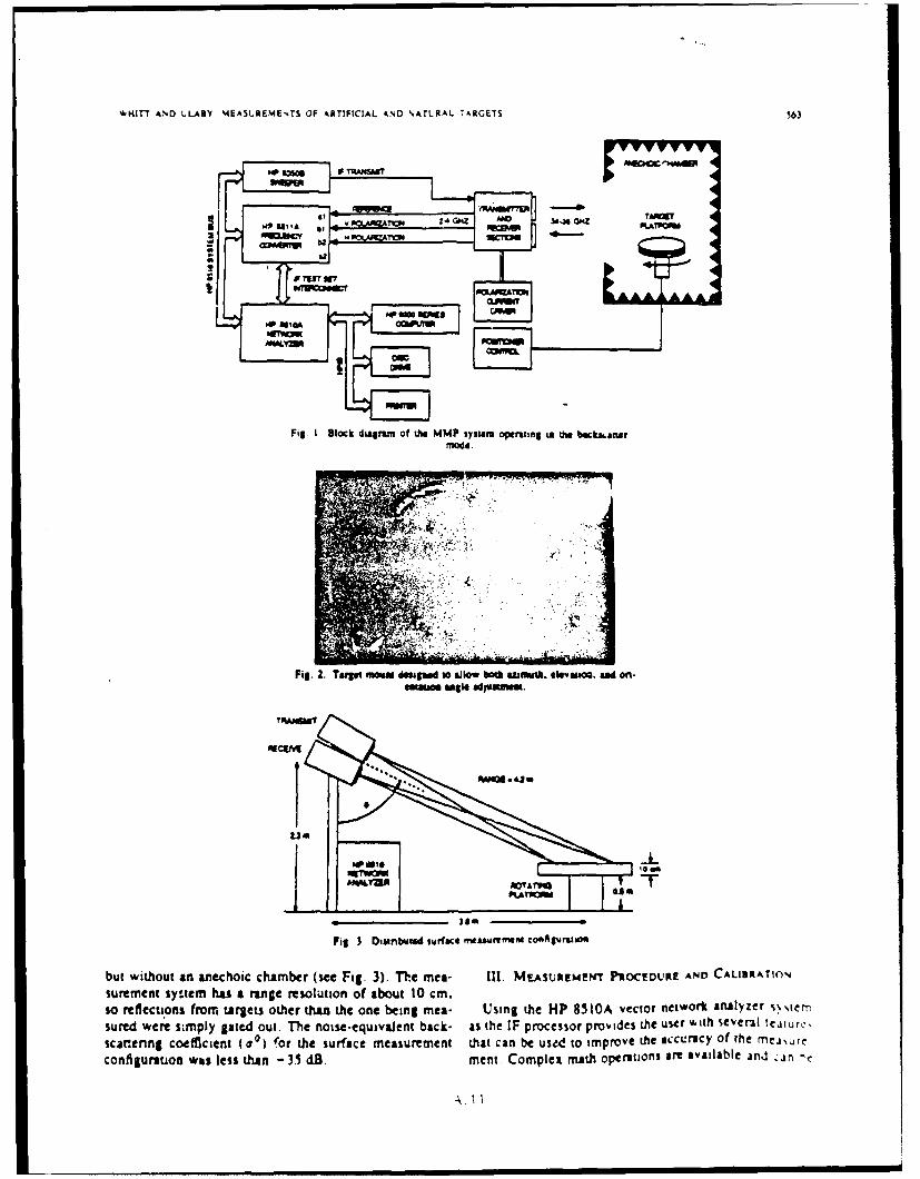


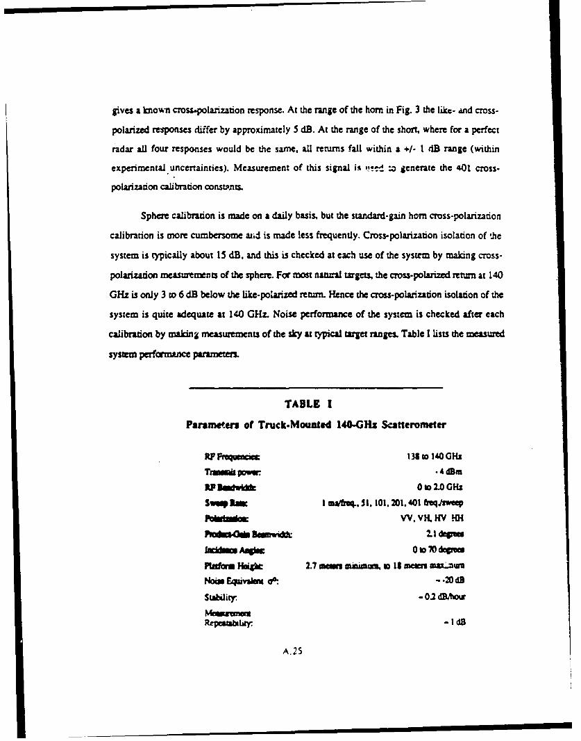


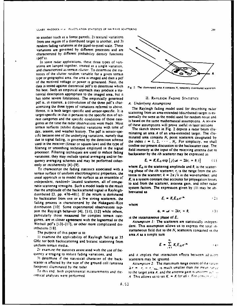


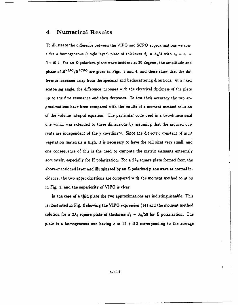


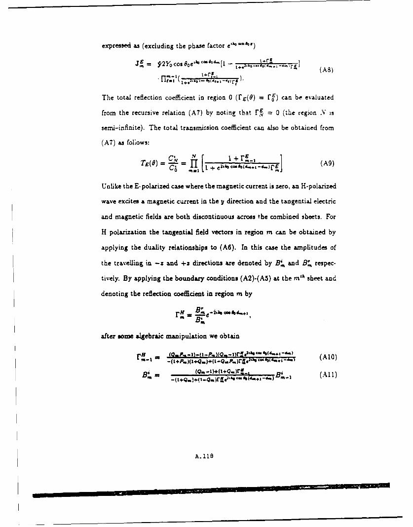


![Documento Ummo D52 [IU1], Concepto de Simetria](https://static.documents.pub/doc/80x56/55cf8a9555034654898bffc7/documento-ummo-d52-iu1-concepto-de-simetria.jpg)


