Chapter 6 Surface and Volume Clutter -...

© 200

Chapter 6 Surface and Volume Clutter

6.1. Clutter DefinitionClutter is a term used to describe any object that may generate unwanted

radar returns that may interfere with normal radar operations. Parasitic returns that enter the radar through the antenna�s main lobe are called main lobe clut-ter; otherwise they are called sidelobe clutter. Clutter can be classified into two main categories: surface clutter and airborne or volume clutter. Surface clutter includes trees, vegetation, ground terrain, man-made structures, and sea sur-face (sea clutter). Volume clutter normally has a large extent (size) and includes chaff, rain, birds, and insects. Surface clutter changes from one area to another, while volume clutter may be more predictable.

Clutter echoes are random and have thermal noise-like characteristics because the individual clutter components (scatterers) have random phases and amplitudes. In many cases, the clutter signal level is much higher than the receiver noise level. Thus, the radar�s ability to detect targets embedded in high clutter background depends on the Signal-to-Clutter Ratio (SCR) rather than the SNR.

White noise normally introduces the same amount of noise power across all radar range bins, while clutter power may vary within a single range bin. Since clutter returns are target-like echoes, the only way a radar can distinguish tar-get returns from clutter echoes is based on the target RCS , and the antici-pated clutter RCS (via clutter map). Clutter RCS can be defined as the equivalent radar cross section attributed to reflections from a clutter area, . The average clutter RCS is given by

(6.1)

σtσc

Ac

σc σ0Ac=

4 by Chapman & Hall/CRC CRC Press LLC

© 200

where is the clutter scattering coefficient, a dimensionless quan-tity that is often expressed in dB. Some radar engineers express in terms of squared centimeters per squared meter. In these cases, is higher than normal.

6.2. Surface ClutterSurface clutter includes both land and sea clutter, and is often called area

clutter. Area clutter manifests itself in airborne radars in the look-down mode. It is also a major concern for ground-based radars when searching for targets at low grazing angles. The grazing angle is the angle from the surface of the earth to the main axis of the illuminating beam, as illustrated in Fig. 6.1.

Three factors affect the amount of clutter in the radar beam. They are the grazing angle, surface roughness, and the radar wavelength. Typically, the clut-ter scattering coefficient is larger for smaller wavelengths. Fig. 6.2 shows a sketch describing the dependency of on the grazing angle. Three regions are identified; they are the low grazing angle region, flat or plateau region, and the high grazing angle region.

σ0 m2 m2⁄( )σ0

σ0 40dB

ψg

ψgearth surface

Figure 6.1. Definition of grazing angle.

σ0

σ0

σ0 dB

grazing angle

0dB

critical angle 60°>

Figure 6.2. Clutter regions.

high grazingangle regionplateau region

low grazingangle region


© 200

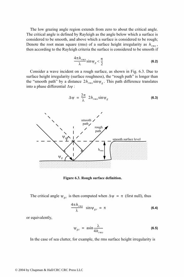
The low grazing angle region extends from zero to about the critical angle. The critical angle is defined by Rayleigh as the angle below which a surface is considered to be smooth, and above which a surface is considered to be rough; Denote the root mean square (rms) of a surface height irregularity as , then according to the Rayleigh criteria the surface is considered to be smooth if

(6.2)

Consider a wave incident on a rough surface, as shown in Fig. 6.3. Due to surface height irregularity (surface roughness), the �rough path� is longer than the �smooth path� by a distance . This path difference translates into a phase differential :

(6.3)

The critical angle is then computed when (first null), thus

(6.4)

or equivalently,

(6.5)

In the case of sea clutter, for example, the rms surface height irregularity is

hrms

4πhrms

λ----------------- ψgsin π

2---<

2hrms ψgsin∆ψ

∆ψ 2πλ

------ 2hrms ψgsin=

ψg

ψg

smoothpath

roughpath

smooth surface level

hrms

Figure 6.3. Rough surface definition.

ψgc ∆ψ π=

4πhrms

λ----------------- ψgcsin π=

ψgcλ

4hrms-------------asin=


© 200

(6.6)

where is the sea state, which is tabulated in several cited references. The sea state is characterized by the wave height, period, length, particle velocity, and wind velocity. For example, refers to a moderate sea state, where in this case the wave height is approximately between

, the wave period 6.5 to 4.5 seconds, wave length , wave velocity , and wind

velocity .

Clutter at low grazing angles is often referred to as diffuse clutter, where there are a large number of clutter returns in the radar beam (non-coherent reflections). In the flat region the dependency of on the grazing angle is minimal. Clutter in the high grazing angle region is more specular (coherent reflections) and the diffuse clutter components disappear. In this region the smooth surfaces have larger than rough surfaces, opposite of the low graz-ing angle region.

6.2.1. Radar Equation for Area Clutter - Airborne Radar

Consider an airborne radar in the look-down mode shown in Fig. 6.4. The intersection of the antenna beam with the ground defines an elliptically shaped footprint. The size of the footprint is a function of the grazing angle and the antenna 3dB beamwidth , as illustrated in Fig. 6.5. The footprint is divided into many ground range bins each of size , where is the pulsewidth.

From Fig. 6.5, the clutter area is

(6.7)

hrms 0.025 0.046 Sstate1.72+≈

Sstate

Sstate 3=

0.9144 to 1.2192 m1.9812 to 33.528 m 20.372 to 25.928 Km hr⁄

22.224 to 29.632 Km hr⁄

σ0

σ0

θ3dBcτ 2⁄( ) ψgsec τ

Ac

Ac Rθ3dBcτ2----- ψgsec≈

ψg

Figure 6.4. Airborne radar in the look-down mode.

Ac

footprint

R

θ3dB


© 200

The power received by the radar from a scatterer within is given by the radar equation as

(6.8)

where, as usual, is the peak transmitted power, is the antenna gain, is the wavelength, and is the target RCS. Similarly, the received power from clutter is

(6.9)

where the subscript is used for area clutter. Substituting Eq. (6.1) for into Eq. (6.9), we can then obtain the SCR for area clutter by dividing Eq. (6.8) by Eq. (6.9). More precisely,

(6.10)

Example:

Consider an airborne radar shown in Fig. 6.4. Let the antenna 3dB beam-width be , the pulsewidth , range , and

cτ2-----

AcRθ3dB

Rθ3dB ψgcsc

cτ2----- ψgsec

ψg

Figure 6.5. Footprint definition.

Ac

StPtG

2λ2σt

4π( )3R4-----------------------=

Pt G λσt

SCPtG

2λ2σc

4π( )3R4------------------------=

C σc

SCR( )C2σt ψgcos

σ0θ3dBRcτ---------------------------=

θ3dB 0.02rad= τ 2µs= R 20Km=


© 200

grazing angle . The target RCS is . Assume that the clut-ter reflection coefficient is . Compute the SCR.

Solution:

The SCR is given by Eq. (6.10) as

It follows that

Thus, for reliable detection the radar must somehow increase its SCR by at least , where is on the order of or better.

6.2.2. Radar Equation for Area Clutter - Ground Based Radar

Again the received power from clutter is also calculated using Eq. (6.9). However, in this case the clutter RCS is computed differently. It is

(6.11)

where is the main beam clutter RCS and is the sidelobe clutter RCS, as illustrated in Fig. 6.6.

ψg 20°= σt 1m2=σ0 0.0136=

SCR( )C2σt ψgcos

σ0θ3dBRcτ--------------------------- ⇒=

SCR( )C2( ) 1( ) 20°cos( )

0.0136( ) 0.02( ) 20000( ) 3 108×( ) 2 10 6�×( )--------------------------------------------------------------------------------------------------------- 5.76 10 4�×= =

SCR( )C 32.4dB�=

32 X+( )dB X 13 to 15dB

σc

σc σMBc σSLc+=

σMBc σSLc

Figure 6.6. Geometry for ground based radar clutter

main beam cluttersidelobe

clutter


© 200

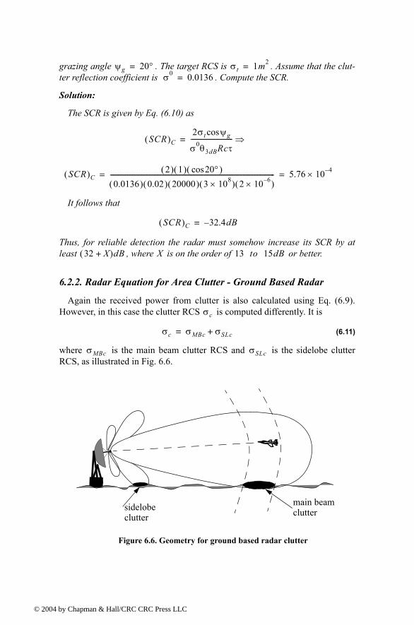
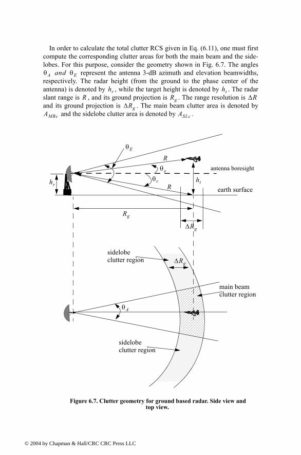
In order to calculate the total clutter RCS given in Eq. (6.11), one must first compute the corresponding clutter areas for both the main beam and the side-lobes. For this purpose, consider the geometry shown in Fig. 6.7. The angles

represent the antenna 3-dB azimuth and elevation beamwidths, respectively. The radar height (from the ground to the phase center of the antenna) is denoted by , while the target height is denoted by . The radar slant range is , and its ground projection is . The range resolution is and its ground projection is . The main beam clutter area is denoted by

and the sidelobe clutter area is denoted by .

θA and θE

hr htR Rg ∆R

∆RgAMBc ASLc

earth surfacehr

ht

R

Rg

θE

θe

θr

∆Rg

∆Rg

θA

sidelobeclutter region

sidelobeclutter region

main beamclutter region

Figure 6.7. Clutter geometry for ground based radar. Side view and top view.

R

antenna boresight


© 200

From Fig. 6.7 the following relations can be derived

(6.12)

(6.13)

(6.14)

where is the radar range resolution. The slant range ground projection is

(6.15)

It follows that the main beam and the sidelobe clutter areas are

(6.16)

(6.17)

Assume a radar antenna beam of the form

(6.18)

(6.19)

Then the main beam clutter RCS is

(6.20)

and the sidelobe clutter RCS is

(6.21)

where the quantity is the root-mean-square (rms) for the antenna side-lobe level.

Finally, in order to account for the variation of the clutter RCS versus range, one can calculate the total clutter RCS as a function of range. It is given by

(6.22)

where is the radar range to the horizon calculated as

θr hr R⁄( )asin=

θe ht hr�( ) R⁄( )asin=

∆Rg ∆R θrcos=

∆R

Rg R θrcos=

AMBc ∆Rg Rg θA=

ASLc ∆Rg πRg=

G θ( )

G θ( ) 2.776θ2

θE2

-------------------�

exp= Gaussian⇒

G θ( )

2.78 θθE-----

sin

2.78 θθE-----

------------------------------

2

0

θπθE

2.78----------≤;

elsewhere;

=x( )sin

x---------------

2⇒

σMBc σ0AMBcG2 θe θr+( ) σ0∆Rg Rg θAG2 θe θr+( )= =

σSLc σ0ASLc SLrms( )2 σ0∆Rg πRg SLrms( )2= =

SLrms

σc R( )σMBc σSLc+

1 R Rh⁄( )4+( )-----------------------------------=

Rh


© 200

(6.23)

where is the Earth�s radius equal to . The denominator in Eq. (6.22) is put in that format in order to account for refraction and for round (spherical) Earth effects.

The radar SNR due to a target at range is

(6.24)

where, as usual, is the peak transmitted power, is the antenna gain, is the wavelength, is the target RCS, is Boltzman�s constant, is the effective noise temperature, is the radar operating bandwidth, is the receiver noise figure, and is the total radar losses. Similarly, the Clutter-to-Noise (CNR) at the radar is

(6.25)

where the is calculated using Eq. (6.21).

When the clutter statistic is Gaussian, the clutter signal return and the noise return can be combined, and a new value for determining the radar measure-ment accuracy is derived from the Signal-to-Clutter+Noise-Ratio, denoted by SIR. It is given by

(6.26)

Note that the is computed by dividing Eq.(6.24) by Eq. (6.25).

MATLAB Function �clutter_rcs.m�

The function �clutter_rcs.m� implements Eq. (6.22); it is given in Listing 6.1 in Section 6.6. It also generates plots of the clutter RCS and the CNR ver-sus the radar slant range. Its outputs include the clutter RCS in dBsm and the CNR in dB. The syntax is as follows:

[sigmaC,CNR] = clutter_rcs(sigma0, thetaE, thetaA, SL, range, hr, ht, pt, f0, b, t0, f, l, ant_id)

where

Rh8hrre

3-------------=

re 6371Km

R

SNRPtG

2λ2σt

4π( )3R4kToBFL----------------------------------------=

Pt G λσt k T0

B FL

CNRPtG

2λ2σc

4π( )3R4kToBFL----------------------------------------=

σc

SIR 11

SNR----------- 1

SCR-----------+

-----------------------------=

SCR


© 200

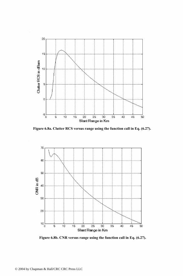
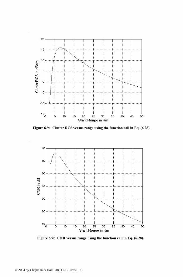
A GUI called �clutter_rcs_gui� was developed for this function. Executing this GUI generates plots of the and versus range. Figure 6.8 shows typical plots produced by this GUI using the antenna pattern defined in Eq. (6.18). Figure 6.9 is similar to Fig. 6.8 except in this case Eq. (6.19) is used for the antenna pattern. Note that the dip in the clutter RCS (at very close range) occurs at the grazing angle corresponding to the null between the main beam and the first sidelobe. Fig. 6.9c shows the GUI workspace associated with this function.

In order to reproduce those two figures use the following MATLAB calls:

[sigmaC,CNR] = clutter_rcs(-20, 2, 1, -20, linspace(2,50,100), 3, 100, 75, 5.6e9, 1e6, 290, 6, 10, 1) (6.27)

[sigmaC,CNR] = clutter_rcs(-20, 2, 1, -25, linspace(2,50,100), 3, 100, 100, 5.6e9, 1e6, 290, 6, 10, 2) (6.28)

Symbol Description Units Status

sigma0 clutter back scatterer coefficient dB input

thetaE antenna 3dB elevation beamwidth degrees input

thetaA antenna 3dB azimuth beamwidth degrees input

SL antenna sidelobe level dB input

range range; can be a vector or a single value Km input

hr radar height meters input

ht target height meters input

pt radar peak power KW input

f0 radar operating frequency Hz input

b bandwidth Hz input

t0 effective noise temperature Kelvins input

f noise figure dB input

l radar losses dB input

ant_id 1 for (sin(x)/x)^2 pattern

2 for Gaussian pattern

none input

sigmac clutter RCS; can be either vector or sin-gle value depending on �range�

dB output

CNR clutter to noise ratio; can be either vec-tor or single value depending on

�range�

dB output

σc CNR


© 200

Figure 6.8a. Clutter RCS versus range using the function call in Eq. (6.27).

Figure 6.8b. CNR versus range using the function call in Eq. (6.27).


© 200

Figure 6.9a. Clutter RCS versus range using the function call in Eq. (6.28).

Figure 6.9b. CNR versus range using the function call in Eq. (6.28).


© 200

Figure 6.9c. GUI workspace for �clutter_rcs_gui.m�.


© 200

6.3. Volume ClutterVolume clutter has large extents and includes rain (weather), chaff, birds,

and insects. The volume clutter coefficient is normally expressed in square meters (RCS per resolution volume). Birds, insects, and other flying particles are often referred to as angle clutter or biological clutter.

As mentioned earlier, chaff is used as an ECM technique by hostile forces. It consists of a large number of dipole reflectors with large RCS values. Histori-cally, chaff was made of aluminum foil; however, in recent years most chaff is made of the more rigid fiberglass with conductive coating. The maximum chaff RCS occurs when the dipole length is one half the radar wavelength.

Weather or rain clutter is easier to suppress than chaff, since rain droplets can be viewed as perfect small spheres. We can use the Rayleigh approxima-tion of a perfect sphere to estimate the rain droplets� RCS. The Rayleigh approximation, without regard to the propagation medium index of refraction is:

(6.29)

where , and is radius of a rain droplet.

Electromagnetic waves when reflected from a perfect sphere become strongly co-polarized (have the same polarization as the incident waves). Con-sequently, if the radar transmits, for example, a right-hand-circular (RHC) polarized wave, then the received waves are left-hand-circular (LHC) polar-ized, because they are propagating in the opposite direction. Therefore, the back-scattered energy from rain droplets retains the same wave rotation (polar-ization) as the incident wave, but has a reversed direction of propagation. It follows that radars can suppress rain clutter by co-polarizing the radar transmit and receive antennas.

Denote as RCS per unit resolution volume . It is computed as the sum of all individual scatterers RCS within the volume,

(6.30)

where is the total number of scatterers within the resolution volume. Thus, the total RCS of a single resolution volume is

(6.31)

L

σ 9πr2 kr( )4= r λ«

k 2π λ⁄= r

η VW

η σi

i 1=

N

∑=

N

σW σiVW

i 1=

N

∑=


© 200

A resolution volume is shown in Fig. 6.10, and is approximated by

(6.32)

where , are, respectively, the antenna azimuth and elevation beamwidths in radians, is the pulsewidth in seconds, is speed of light, and is range.

Consider a propagation medium with an index of refraction . The rain droplet RCS approximation in this medium is

(6.33)

where

(6.34)

and is the droplet diameter. For example, temperatures between and yield

(6.35)

and for ice Eq. (6.33) can be approximated by

(6.36)

Substituting Eq. (6.33) into Eq. (6.30) yields

VWπ8---θaθeR2cτ≈

θa θeτ c R

θe

θa

cτ2-----

R

Figure 6.10. Definition of a resolution volume.

m ith

σiπ5

λ4-----K2Di

6≈

K2 m2 1�

m2 2+----------------

2=

Di ith 32°F68°F

σi 0.93π5

λ4-----Di

6≈

σi 0.2π5

λ4-----Di

6≈


© 200

(6.37)

where the weather clutter coefficient is defined as

(6.38)

In general, a rain droplet diameter is given in millimeters and the radar reso-lution volume is expressed in cubic meters; thus the units of are often expressed in .

6.3.1. Radar Equation for Volume Clutter

The radar equation gives the total power received by the radar from a tar-get at range as

(6.39)

where all parameters in Eq. (6.39) have been defined earlier. The weather clut-ter power received by the radar is

(6.40)

Using Eq. (6.31) and Eq. (6.32) in Eq. (6.40) and collecting terms yield

(6.41)

The SCR for weather clutter is then computed by dividing Eq. (6.39) by Eq. (6.41). More precisely,

(6.42)

where the subscript is used to denote volume clutter.

η π5

λ4-----K2Z=

Z

Z Di6

i 1=

N

∑=

Zmillimeter6 m3⁄

σtR

StPtG

2λ2σt

4π( )3R4-----------------------=

SWPtG

2λ2σW

4π( )3R4-------------------------=

SWPtG

2λ2

4π( )3R4-------------------- π

8---R2θaθecτ σi

i 1=

N

∑=

SCR( )VSt

SW------

8σt

πθaθecτR2 σi

i 1=

N

∑-----------------------------------------= =

V


© 200

Example:

A certain radar has target RCS , pulsewidth , antenna beamwidth . Assume the detection range to be , and compute the SCR if .

Solution:

From Eq. (6.42) we have

Substituting the proper values we get

.

6.4. Clutter Statistical ModelsSince clutter within a resolution cell or volume is composed of a large num-

ber of scatterers with random phases and amplitudes, it is statistically described by a probability distribution function. The type of distribution depends on the nature of clutter itself (sea, land, volume), the radar operating frequency, and the grazing angle.

If sea or land clutter is composed of many small scatterers when the proba-bility of receiving an echo from one scatterer is statistically independent of the echo received from another scatterer, then the clutter may be modeled using a Rayleigh distribution,

(6.43)

where is the mean squared value of .

The log-normal distribution best describes land clutter at low grazing angles. It also fits sea clutter in the plateau region. It is given by

(6.44)

σt 0.1m2= τ 0.2µs=θa θe 0.02radians= =

R 50Km= σi∑ 1.6 10 8�× m2 m3⁄( )=

SCR( )V8σt

πθaθecτR2 σi

i 1=

N

∑-----------------------------------------=

SCR( )V8( ) 0.1( )

π 0.02( )2 3 108×( ) 0.2 10 6�×( ) 50 103×( )2

1.6 10 8�×( )----------------------------------------------------------------------------------------------------------------------------------- 0.265= =

SCR( )V 5.76� dB=

f x( ) 2xx0------ x2�

x0-------- x 0≥;exp=

x0 x

f x( ) 1σ 2π x--------------------- �

xln xmln�( )2

2σ2---------------------------------

exp x 0>;=


© 200

where is the median of the random variable , and is the standard devi-ation of the random variable .

The Weibull distribution is used to model clutter at low grazing angles (less than five degrees) for frequencies between and . The Weibull proba-bility density function is determined by the Weibull slope parameter (often tabulated) and a median scatter coefficient , and is given by

(6.45)

where is known as the shape parameter. Note that when the Weibull distribution becomes a Rayleigh distribution.

6.5. �MyRadar� Design Case Study - Visit 6

6.5.1. Problem Statement

Analyze the impact of ground clutter on �MyRadar� design case study. Assume a Gaussian antenna pattern. Assume that the radar height is 5 meters. Consider an antenna sidelobe level and a ground clutter coef-ficient . What conclusions can you draw about the radar�s ability to maintain proper detection and track of both targets? Assume a radar height .

6.5.2. A Design

From the design processes established in Chapters 1 and 2, it was determined that the minimum single pulse SNR required to accomplish the design objec-tives was when non-coherent integration (4 pulses) and cumula-tive detection were used. Factoring in the surface clutter will degrade the SIR. However, one must maintain in order to achieve the desired prob-ability of detection.

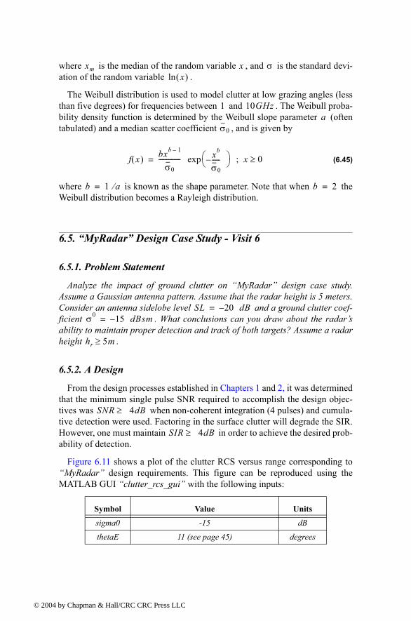
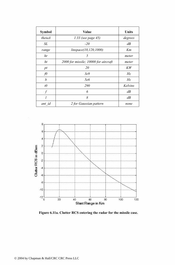
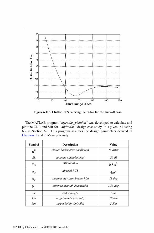
Figure 6.11 shows a plot of the clutter RCS versus range corresponding to �MyRadar� design requirements. This figure can be reproduced using the MATLAB GUI �clutter_rcs_gui� with the following inputs:

Symbol Value Units

sigma0 -15 dB

thetaE 11 (see page 45) degrees

xm x σx( )ln

1 10GHza

σ0

f x( ) bxb 1�

σ0-------------- xb

σ0-----�

x 0≥;exp=

b 1 a⁄= b 2=

SL 20 dB�=σ0 15 dBsm�=

hr 5m≥

SNR 4dB≥

SIR 4dB≥


© 200

thetaA 1.33 (see page 45) degrees

SL -20 dB

range linspace(10,120,1000) Km

hr 5 meter

ht 2000 for missile; 10000 for aircraft meter

pt 20 KW

f0 3e9 Hz

b 5e6 Hz

t0 290 Kelvins

f 6 dB

l 8 dB

ant_id 2 for Gaussian pattern none

Symbol Value Units

Figure 6.11a. Clutter RCS entering the radar for the missile case.


© 200

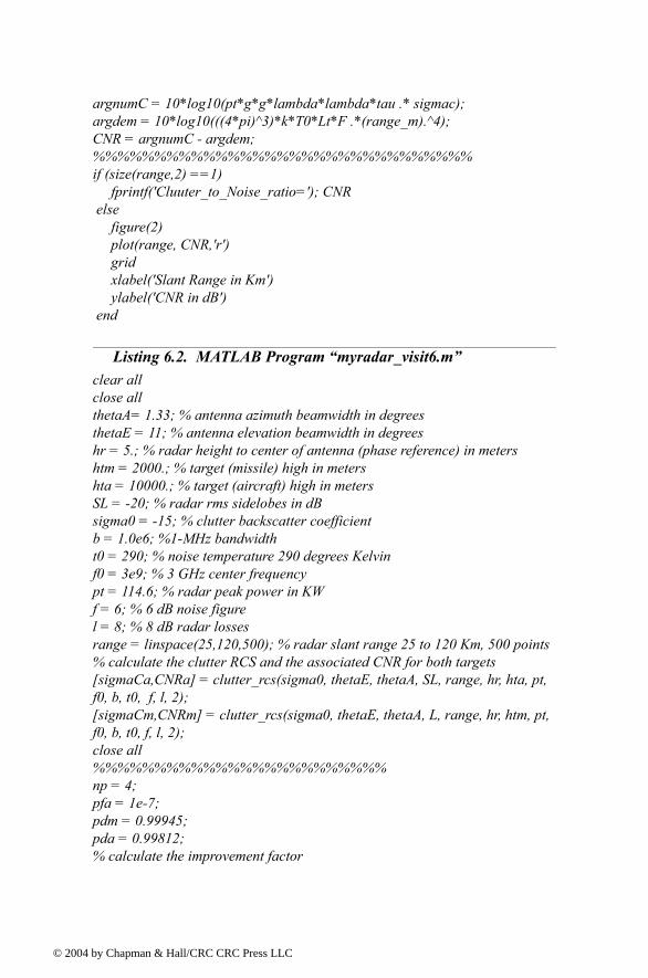
The MATLAB program �myradar_visit6.m� was developed to calculate and plot the CNR and SIR for �MyRadar� design case study. It is given in Listing 6.2 in Section 6.6. This program assumes the design parameters derived in Chapters 1 and 2. More precisely:

Symbol Description Value

clutter backscatter coefficient -15 dBsm

SL antenna sidelobe level -20 dB

missile RCS

aircraft RCS

antenna elevation beamwidth 11 deg

antenna azimuth beamwidth 1.33 deg

hr radar height 5 m

hta target height (aircraft) 10 Km

htm target height (missile) 2 Km

Figure 6.11b. Clutter RCS entering the radar for the aircraft case.

σ0

σm 0.5m2

σa 4m2

θE

θA


© 200

Figure 6.12 shows a plot of the CNR and the SIR associated with the mis-sile. Figure 6.13 is similar to Fig. 6.12 except it is for the aircraft case. It is clear from these figures that the required SIR has been degraded significantly for the missile case and not as much for the aircraft case. This should not be surprising, since the missile�s altitude is much smaller than that of the aircraft. Without clutter mitigation, the missile would not be detected at all. Alterna-tively, the aircraft detection is compromised at . Clutter mitigation is the subject of the next chapter.

radar peak power 20 KW

radar operating frequency 3GHz

effective noise temperature 290 degrees Kelvin

noise figure 6 dB

L radar total losses 8 dB

Uncompressed pulsewidth 20 microseconds

Symbol Description Value

Pt

f0

T0

F

τ′

R 80Km≤

Figure 6.12. SNR, CNR, and SIR versus range for the missile case.


© 200

6.6. MATLAB Program and Function ListingsThis section presents listings for all MATLAB programs/functions used in

this chapter. The user is advised to rerun these programs with different input parameters.

Listing 6.1. MATALB Function �clutter_rcs.m�function [sigmaC,CNR] = clutter_rcs(sigma0, thetaE, thetaA, SL, range, hr, ht, pt, f0, b, t0, f, l,ant_id)% This function calculates the clutter RCS and the CNR for a ground based radar.clight = 3.e8; % speed of light in meters per secondlambda = clight /f0;thetaA_deg = thetaA;thetaE_deg = thetaE;thetaA = thetaA_deg * pi /180; % antenna azimuth beamwidth in radiansthetaE = thetaE_deg * pi /180.; % antenna elevation beamwidth in radiansre = 6371000; % earth radius in metersrh = sqrt(8.0*hr*re/3.); % range to horizon in meters

Figure 6.13. SNR, CNR and SIR versus range for the aircraft case.


© 200

SLv = 10.0^(SL/10); % radar rms sidelobes in voltssigma0v = 10.0^(sigma0/10); % clutter backscatter coefficient tau = 1/b; % pulsewidth deltar = clight * tau / 2.; % range resolution for unmodulated pulse%%%%%%%%%%%%%%%%%%%%%%%%%%%%%%range_m = 1000 .* range; % range in meters%%%%%%%%%%%%%%%%%%%%%%%%%%%%%%thetar = asin(hr ./ range_m);thetae = asin((ht-hr) ./ range_m);propag_atten = 1. + ((range_m ./ rh).^4); % propagation attenuation due to round earthRg = range_m .* cos(thetar);deltaRg = deltar .* cos(thetar);theta_sum = thetae + thetar;% use sinc^2 antenna pattern when ant_id=1% use Gaussian antenna pattern when ant_id=2if(ant_id ==1) % use sinc^2 antenna pattern ant_arg = (2.78 * theta_sum ) ./ (pi*thetaE); gain = (sinc(ant_arg)).^2;else gain = exp(-2.776 .*(theta_sum./thetaE).^2);end% compute sigmacsigmac = (sigma0v .* Rg .* deltaRg) .* (pi * SLv * SLv + thetaA .* gain.^2) ./ propag_atten;sigmaC = 10*log10(sigmac);%%%%%%%%%%%%%%%%%%%%%%%%%%%%%%%%%%%if (size(range,2)==1) fprintf('Sigma_Clutter='); sigmaCelse figure(1) plot(range, sigmaC) grid xlabel('Slant Range in Km') ylabel('Clutter RCS in dBsm')end%%%%%%%%%%%%%%%%%%%%%%%%%%%%%%%%%% Calculate CNRpt = pt * 1000;g = 26000 / (thetaA_deg*thetaE_deg); % antenna gainF = 10.^(f/10); % noise figure is 6 dBLt = 10.^(l/10); % total radar losses 13 dBk = 1.38e-23; % Boltzman�s constantT0 = t0; % noise temperature 290K


© 200

argnumC = 10*log10(pt*g*g*lambda*lambda*tau .* sigmac);argdem = 10*log10(((4*pi)^3)*k*T0*Lt*F .*(range_m).^4);CNR = argnumC - argdem;%%%%%%%%%%%%%%%%%%%%%%%%%%%%%%%if (size(range,2) ==1) fprintf('Cluuter_to_Noise_ratio='); CNR else figure(2) plot(range, CNR,'r') grid xlabel('Slant Range in Km') ylabel('CNR in dB') end

Listing 6.2. MATLAB Program �myradar_visit6.m�clear allclose allthetaA= 1.33; % antenna azimuth beamwidth in degreesthetaE = 11; % antenna elevation beamwidth in degreeshr = 5.; % radar height to center of antenna (phase reference) in metershtm = 2000.; % target (missile) high in metershta = 10000.; % target (aircraft) high in metersSL = -20; % radar rms sidelobes in dBsigma0 = -15; % clutter backscatter coefficient b = 1.0e6; %1-MHz bandwidth t0 = 290; % noise temperature 290 degrees Kelvinf0 = 3e9; % 3 GHz center frequencypt = 114.6; % radar peak power in KWf = 6; % 6 dB noise figurel = 8; % 8 dB radar lossesrange = linspace(25,120,500); % radar slant range 25 to 120 Km, 500 points% calculate the clutter RCS and the associated CNR for both targets[sigmaCa,CNRa] = clutter_rcs(sigma0, thetaE, thetaA, SL, range, hr, hta, pt, f0, b, t0, f, l, 2);[sigmaCm,CNRm] = clutter_rcs(sigma0, thetaE, thetaA, L, range, hr, htm, pt, f0, b, t0, f, l, 2);close all%%%%%%%%%%%%%%%%%%%%%%%%np = 4;pfa = 1e-7;pdm = 0.99945;pda = 0.99812;% calculate the improvement factor


© 200

Im = improv_fac(np,pfa, pdm);Ia = improv_fac(np, pfa, pda);% calculate the integration lossLm = 10*log10(np) - Im;La = 10*log10(np) - Ia;pt = pt * 1000; % peak power in wattsrange_m = 1000 .* range; % range in metersg = 34.5139; % antenna gain in dBsigmam = 0.5; % missile RCS m squaredsigmaa = 4; % aircraft RCS m squarednf = f; %noise figure in dBloss = l; % radar losses in dBlosstm = loss + Lm; % total loss for missilelossta = loss + La; % total loss for aircraft% modify pt by np*pt to account for pulse integrationSNRm = radar_eq(np*pt, f0, g, sigmam, t0, b, nf, losstm, range_m);SNRa = radar_eq(np*pt, f0, g, sigmaa, t0, b, nf, lossta, range_m);snrm = 10.^(SNRm./10);snra = 10.^(SNRa./10);cnrm = 10.^(CNRm./10);cnra = 10.^(CNRa./10);SIRm = 10*log10(snrm ./ (1+cnrm));SIRa = 10*log10(snra ./ (1+cnra));%%%%%%%%%%%%%%%%%%%%%%%%%%%%%%%figure(3)plot(range, SNRm,'k', range, CNRm,'k :', range,SIRm,'k -.')gridlegend('Desired SNR; from Chapter 5','CNR','SIR')xlabel('Slant Range in Km')ylabel('dB')title('Missile case; 21-frame cumulative detection')%%%%%%%%%%%%%%%%%%%%%%%%%%%%%%%%%%%%%%%%%%figure(4)plot(range, SNRa,'k', range, CNRa,'k :', range,SIRa,'k -.')gridlegend('Desired SNR; from Chapter 5','CNR','SIR')xlabel('Slant Range in Km')ylabel('dB')title('Aircraft case; 21-frame cumulative detection')


Date post:	05-Jun-2018
Category:	Documents
Upload:	hadieu
View:	233 times
Download:	0 times

Chapter 6 Surface and Volume Clutter -...

Documents