9/2004Strickler, et. al1 Reconstruction of Modular Coil Shape and Control of Vacuum Islands in NCSX...

9/2004 Strickler, et. al 1

Reconstruction of Modular Coil Shapeand Control of Vacuum Islands in NCSX

D. Strickler, S. Hirshman, B. Nelson, D. Williamson, L. Berry, J. Lyon

Oak Ridge National Laboratory9/2004


Topics

1. Determination of modular coil shape from

magnetic field measurements

2. Optimization of the vacuum magnetic field configuration with respect to coil

orientation and currents.


1. Shape reconstruction of (as-built) modular

coils from magnetic measurements

• Linear method– Find corrections to design coil coordinates– SVD

• Nonlinear method– Parameterization of coil centerline– Fourier or cubic spline representation – Use Levenberg-Marquardt to find coefficients


Measure B=(Bx,By,Bz) or │B│ on 3D grid enclosing design coil shape

Example: NCSX modular coil M1• Uniform grid spacing of 5 cm in each coordinate direction • ~3500 field measurement points within 20–25 cm of design coil centerline

Side view Top view


Test procedures on NCSX modular coil M1 with known shape distortion

Sine, cosine coil distortions :• ΔR = δr sin (mθ)• Δφ = δφ sin (mθ)• ΔZ = δz sin (mθ)

Design coil (solid)Distorted coil (dashed)

m=5δr = δφ = δz = 5 mm

Side view Top view

Include random error in:•Magnetic field meaurements•Location of measurements


x0 = [x01,y01,z01, … ,x0n, y0n, z0n]T ideal (design) coil coordinates

B0 = B(x0) magnetic field of ideal coil over 3D grid

x0 + Δx coordinates of actual coil (manufactured)

B1 = B(x0 + Δx) magnetic field of actual coil (measured)

B1 – B0 = Δb ≈ BΔx B = dB/dx is MxN Jacobian matrix

B = U∑VT SVD

Δx = ∑σn ≠ 0 (unT Δb)vn/ σn least-squares solution for Δx

Drop ‘small’ singular values σn to stabilize solution, making it less sensitiveto data vector Δb

Linear MethodSolve for coordinates of coil winding center


Linear shape reconstruction of distorted modular coil M1• sin(5θ) distortion with δr = δφ = δz = 2mm• Random measurement error in field: δB/Bmax ≤ 1.e-5, grid : dx, dy, dz ≤ 0.1 mm• Solution depends on number of singular values retained (Nσ)• Error in coil coord.: χcoil = { [ ∑ (xn – xn

(dist))2 + (yn – yn(dist))2 + (zn – zn

(dist))2 ] / N }1/2

σmin /σmax = 0.001, Nσ = 213 σmin /σmax = 0.015, Nσ = 132

Field error χ = 2.281e-5 TΧcoil = 3.052e-3

Field error χ = 2.310e-5 TΧcoil = 7.766e-4

Distorted coil (dashed)Reconstruction (solid)



d [mm]δB/Bmax χfield [T] χcoil [m]

0.0 0.0 2.398e-6 7.455e-4

0.0 1.e-5 2.573e-6 7.455e-4

0.1 1.e-5 2.310e-5 7.766e-4

0.5 1.e-5 1.147e-4 1.131e-3

1.0 1.e-5 2.293e-4 2.281e-3

Linear coil shape reconstruction from magnetic field │B│with random error ≤ d in location of field measurements

• sine coil distortion with m=5, δr = δφ = δz = 0.002m• σmin / σmax = 0.015, Nσ = 132


δB/Bmax χfield [T] χcoil [m]

1.e-5 2.310e-5 7.766e-4

5.e-5 2.362e-5 7.769e-4

1.e-4 2.516e-5 7.786e-4

5.e-4 5.480e-5 8.416e-4

1.e-3 1.019e-4 1.019e-3

Linear coil shape reconstruction from magnetic field │B│with random error ≤ δB in field measurement values

• sine coil distortion with m=5, δr = δφ = δz = 0.002m• σmin / σmax = 0.015, Nσ = 132• Error in measurement locations d ≤ 0.1 mm


x = [x(t), y(t), z(t)] coordinates of coil centerline

x(t) = ax0 + ∑ax,kcos(2πkt) + bx,ksin (2πkt) , … Fourier representation

c = [ax0,ax1,bx1, … ,azn, bzn]T vector of coefficients

B = B(c) magnetic field over 3D grid

Minimize χ2 = ║B(c) – B1║2 B1 = field measurements on 3D grid

Nonlinear MethodSolve for coefficients in parameterization of coil winding center

• Levenberg-Marquardt method to solve for coefficients• Initial guess for c based on fit to design coil data• Option in code for cubic spline representation: x(t) = ∑ cx,k Bk(t), …


Sensitivity of solution to initial approximation

• Define design coil by Fourier series (e.g., fit to NCSX modular coil 1 coordinates, total Nc=159 coefficients)

• Create distorted coil by changing single coefficient ( e.g., ay,1 = ay,1

(design) + Δay )

• Reconstruct distorted coil shape from magnetic measurements with initial approximation to solution given by:

• ax,m = ax,m(design) , bx,m = bx,m

(design), etc.., except for ay,1 = ay,1

(design) + (1 – α)Δay

• Let χx = [ ∑ (ax,m– ax,m(design))2 + (bx,m– bx,m

(design) )2 ]1/2 , etc ..


Sensitivity to initial approximation (continued)

αField

error(T)Δay,1(m) Χx(m) Χy(m) Χz(m)

0.01 1.621e-8 0.0100 1.615e-4 1.003e-2 2.142e-4

0.1 1.316e-6 0.0100 1.957e-3 1.001e-2 2.135e-3

0.5 6.242e-5 0.0102 2.083e-2 1.463e-2 2.337e-2

1.0 1.780e-4 0.0077 2.508e-2 1.699e-2 3.373e-2

Design coil +Distorted X

Design coil +Distorted X

m m

am am

α = 0.01 α = 1.0


Design coil (solid)Distorted (dashed)



α = 1.0 α = 0.01


Avg. error in reconstructed coil geometry

• Distorted coil described by N segments, unit tangent vectors ed

• Evaluate solution (approximating field of distorted coil) at N points x• For each point xd on distorted coil, find nearest solution point x*, and perpendicular distance from solution point to distorted coil:

x║ = [( x* – xd )∙ed ]ed

x┴ = x* – xd - x║

d = 1/N ∑i║xi┴║


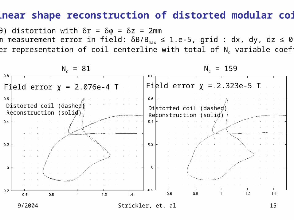
Nonlinear shape reconstruction of distorted modular coil M1

• sin(5θ) distortion with δr = δφ = δz = 2mm• Random measurement error in field: δB/Bmax ≤ 1.e-5, grid : dx, dy, dz ≤ 0.1 mm• Fourier representation of coil centerline with total of Nc variable coefficients


Field error χ = 2.323e-5 T



Nc = 81 Nc = 159


Nonlinear shape reconstruction of distorted modular coil M1

• sin(5θ) distortion with δr = δφ = δz = 2mm• Random measurement error in field: δB/Bmax ≤ 1.e-5• Random error ≤ d in measurement locations : dx, dy, dz



Nc = 159, d = 1.0 mm Nc = 159, d = 0.1 mm




d [mm]δB/Bmax χfield [T] ║c – ccoil║

0.0 0.0 1.994e-6 7.453e-3

0.0 1.e-5 2.243e-6 7.505e-3

0.1 1.e-5 2.332e-5 1.238e-2

0.5 1.e-5 1.158e-4 1.790e-2

1.0 1.e-5 2.368e-4 2.136e-2

Nonlinear coil shape reconstruction from magnetic field │B│with random error ≤ d in location of field measurements

• sine coil distortion with m=5, δr = δφ = δz = 0.002m• ccoil = vector of coefficients in fit to distorted coil coordinates• c = solution vector in nonlinear fit to field of distorted coil


Next

• Apply to multifilament coil with leads

• Test methods on racetrack coil


2. Optimization of the Vacuum Field Configuration

• Vacuum field constraint used in QPS design optimization

• Recent STELLOPT modifications for vacuum field optimization

• Examples


A vacuum field constraint in the STELLOPT / COILOPT codeled to a robust Quasi-Poloidal compact stellaratorconfiguration [1] with improved vacuum properties

•Minimize the normal component of vacuum magnetic field at the full-pressure plasma boundary

- Target B = wB|B•n|/|B|, where: n is normal to the full beta VMEC plasma boundary B is the magnetic field due to the coils

•Last-closed vacuum magnetic flux surface encloses a plasma volume exceeding that of the targeted high equilibrium

•Aspect ratio is maintained as is increased

[1] D.J. Strickler, S.P. Hirshman, D.A Spong, et al., Fusion Science and Technology 45 (Jan. 2004)


QPS vacuum magnetic surface quality improvement

Full-beta (VMEC)plasma boundary

Coil windingsurface

Full plasma boundaryand vacuum surfaces of

QPS configuration withoutthe vacuum constraint

Optimized QPS configuration with vacuum constraint has larger volume of good flux surfaces

Does not targetvacuum island size


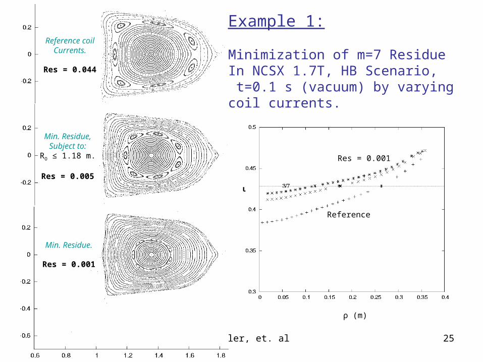
Module (VACOPT) added to stellarator optimization code (STELLOPT) to target resonances in vacuum magnetic field

• Minimize size of vacuum islands resulting from winding geometry errors or displacements due to magnetic loads / joule heating by varying position of modular coils in array.

• Additional variables include rigid-body rotations, shifts about coil centroid, and vacuum field coil currents.

• Targets include residues of prescribed resonances, bounds on variables, and constraints on position of the island O-points.

• Input list now contains poloidal mode number of targeted islands, initial values of vacuum field coil currents, shifts and rotations, and initial positions of control points for each modular coil.

• Output includes positions of control points following optimal shifts / rotations of the modular coils.


•Magnetic field line is described by dx/ds = B(x)

•In cylindrical coordinates (and assuming Bφ ≠ 0), these are reduced to twofield line equations: dR/dφ = RBR/Bφ , dZ/dφ = RBZ/Bφ

•Integrating the field line equations, from a given starting point (e.g. in a symmetryplane), over a toroidal field period, produces a return map X = M(X) (X = [R,Z]t)

•An order m fixed point of M is a periodic orbit: X = Mm(X)

•The dynamics of orbits in the neighborhood of a fixed point are described bythe tangent map: δX = T(δX)

(where T11 = ∂MR/∂R, T12 = ∂MR/∂Z, T21 = ∂MZ/∂R, T22 = ∂MZ/∂Z)

Field Line Equations and Tangent Map


Targeting Magnetic Islands in Vacuum Field Optimization

• Locate O-points of islands (order m fixed points of return map) Xi = (Ri,0)

• Following [1], compute residues of targeted islands

Resi = [2 – trace(T(Xi))]/4

• Optimization

Vary coil currents to minimize targeted residues:

min. χ2 = Σ wiResi2,

Subject to possible constraints, e.g.:

Σ IMOD + ITF = constantRmin ≤ Ri ≤ Rmax, (in prescribed toroidal plane v = vi)

Bounds on modular coil currents

[1] Cary and Hanson, Phys. Fluids 29 (8), 1986


Reference coilCurrents.

Res = 0.044

Min. Residue,Subject to:

RO ≤ 1.18 m.

Res = 0.005

Min. Residue.

Res = 0.001

ρ (m)

ι

Reference

Res = 0.001

Example 1:

Minimization of m=7 ResidueIn NCSX 1.7T, HB Scenario, t=0.1 s (vacuum) by varyingcoil currents.


Example 2: Vacuum field optimization by shifts and rotations about the centroids of modular coils

•Coil currents from 1.7T, high beta scenario at t=0.1s (vacuum)•Minimize m=7 residue•Constrain radius of O-point by R ≤ 1.18m (Z=0)

Res = 0.053 Res = 0.004


Δx (m) Δy (m) Δz (m) θ φ α

M1 0.0005 0.0109 0.0002 0.9866 -0.9471 0.0031

M2 0.0030 -0.0019 0.0151 -0.0494 0.2878 -0.0058

M3 -0.0007 -0.0009 0.0022 0.0669 0.0791 0.0056

Example 2 (cont’d): shifts and rotations about modular coilcentroids for constrained minimization of the m=7 residue

• α measured with respect to unit rotation vector centered at coil centroid with sperical coordinate angles θ, φ.

• Maximum changes in the control points are 1.17cm (M1), 1.58cm (M2), and 0.67cm (M3).


Next

• Test vacuum optimization effect on high beta physics targets

• Correct for non-stellarator symmetric field errors

Date post:	23-Dec-2015
Category:	Documents
Upload:	delilah-mccoy
View:	214 times
Download:	1 times

9/2004Strickler, et. al1 Reconstruction of Modular Coil Shape and Control of Vacuum Islands in NCSX...

Documents