A Bayesian Analysis of Log-Periodic Precursors to Financial Crashes ∗ George Chang † and James Feigenbaum ‡ October 8, 2004 Abstract A large number of papers have been written by physicists document- ing an alleged signature of imminent financial crashes involving so-called log-periodic oscillations—oscillations which are periodic with respect to the logarithm of the time to the crash. In addition to the obvious prac- tical implications of such a signature, log-periodicity has been taken as evidence that financial markets can be modeled as complex statistical- mechanics systems. However, while many log-periodic precursors have been identified, the statistical significance of these precursors and their predictive power remain controversial in part because log-periodicity is ill-suited for study with classical methods. This paper is the first effort to apply Bayesian methods in the testing of log-periodicity. Specifically, we focus on the Johansen-Ledoit-Sornette (JLS) model of log periodicity. Us- ing data from the S&P 500 prior to the October 1987 stock market crash, we find that, if we do not consider crash probabilities, a null hypothe- sis model without log-periodicity outperforms the JLS model in terms of marginal likelihood. If we do account for crash probabilities, which has not been done in the previous literature, the JLS model outperforms the null hypothesis, but only if we ignore the information obtained by standard classical methods. If the JLS model is true, then parameter estimates obtained by curve fitting have small posterior probability. Furthermore, the data set contains negligible information about the oscillation parame- ters, such as the frequency parameter that has received the most attention in the previous literature. JEL Classification: G13, C11. Keywords: Financial crashes; Bayesian inference; log-periodicity. ∗ The authors would like to thank Dave DeJong, John Geweke, Anders Johansen, Jean- Francois Richard, Gene Savin, Pedro Silos, and Chuck Whiteman for suggestions and discus- sions on this topic. † Department of Finance; Bloch School of Business; University of Missouri - Kansas City; Kansas City, MO 64110-2499. E-mail: [email protected]. ‡ Department of Economics; University of Pittsburgh; 4S34 W. W. Posvar Hall; 230 South Bouquet St.; Pittsburgh, PA 15260. E-mail: [email protected]. URL: www.pitt.edu/˜jfeigen. 1
Transcript
A Bayesian Analysis of Log-Periodic Precursors
to Financial Crashes∗
George Chang†and James Feigenbaum‡
October 8, 2004
Abstract
A large number of papers have been written by physicists document-ing an alleged signature of imminent financial crashes involving so-calledlog-periodic oscillations—oscillations which are periodic with respect tothe logarithm of the time to the crash. In addition to the obvious prac-tical implications of such a signature, log-periodicity has been taken asevidence that financial markets can be modeled as complex statistical-mechanics systems. However, while many log-periodic precursors havebeen identified, the statistical significance of these precursors and theirpredictive power remain controversial in part because log-periodicity isill-suited for study with classical methods. This paper is the first effort toapply Bayesian methods in the testing of log-periodicity. Specifically, wefocus on the Johansen-Ledoit-Sornette (JLS) model of log periodicity. Us-ing data from the S&P 500 prior to the October 1987 stock market crash,we find that, if we do not consider crash probabilities, a null hypothe-sis model without log-periodicity outperforms the JLS model in terms ofmarginal likelihood. If we do account for crash probabilities, which hasnot been done in the previous literature, the JLS model outperforms thenull hypothesis, but only if we ignore the information obtained by standardclassical methods. If the JLS model is true, then parameter estimatesobtained by curve fitting have small posterior probability. Furthermore,the data set contains negligible information about the oscillation parame-ters, such as the frequency parameter that has received the most attentionin the previous literature.
∗The authors would like to thank Dave DeJong, John Geweke, Anders Johansen, Jean-Francois Richard, Gene Savin, Pedro Silos, and Chuck Whiteman for suggestions and discus-sions on this topic.
†Department of Finance; Bloch School of Business; University of Missouri - Kansas City;Kansas City, MO 64110-2499. E-mail: [email protected].
‡Department of Economics; University of Pittsburgh; 4S34 W. W. Posvar Hall; 230 SouthBouquet St.; Pittsburgh, PA 15260. E-mail: [email protected]. URL: www.pitt.edu/˜jfeigen.
1
An analogy has often been drawn between crashes in financial marketsand other disruptive events like earthquakes. Recently, a number of physicistshave pursued this qualitative analogy in a more quantitative fashion, suggestingthat such complex “rupture” events can be modeled like phase transitions instatistical mechanical systems. A physical system can exist in different phaseswhen the optimal, energy-minimizing structure of the system is different fordifferent values of the exogenous parameters. The parameter space can thenbe partitioned into regions with different optimal structure. A phase transitionoccurs when the parameters are adjusted in such a way as to cross the bound-ary between two such regions. If x is the distance to the boundary, then anobservable M that varies with x will typically exhibit a power law relationshipM ∼ x−α for some α. If the underlying scaling symmetries of the system arediscrete rather than continuous, the exponent of this power law can be complex(Sornette (1998)). In that case,
and such a periodic relationship with respect to lnx has come to be known asa log-periodic relationship.
In modeling complex rupture events as phase transitions, physicists havesupposed that whatever exogenous parameter x that corresponds to the distanceto the phase boundary varies at a constant rate over time, and so the timeremaining until the critical time tc when the boundary will be crossed can standas a proxy for x. In that case, an observableM(t) of this complex system shouldexhibit a time-series relationship of the form
M(t) ∼ (tc − t)−α cos(ω ln(tc − t) + φ),
where the phase φ is introduced to compensate for the change in units betweenx and tc − t. This idea of viewing rupture events as phase transitions gainedmomentum after such a log-periodic relationship was discovered in historicaldata of ion concentrations within well water near Kobe, Japan prior to the1995 earthquake there (Johansen et al (1996)). Soon afterwards, two groupsindependently discovered such a relationship in the S&P 500 prior to the famousOctober 1987 crash (Feigenbaum and Freund (1996), and Sornette, Johansen,and Bouchaud (1996)) as can be seen in Fig. 1, where the S&P 500 index s(t)is fitted to the specification
This finding sparked an intensive search of time series data on financial prices,and several examples of such log-periodic precursors to financial crashes weresoon identified.1 In addition to the scientific question of whether financial
1For a review of log-periodic research and other examples of how physicists have appliedtheir methods to problems of economic interest, see Feigenbaum (2003). For a more thoroughdiscussion of the evidence in favor of log-periodicity, see Sornette (2003).
2
Figure 1: The S&P 500 from 1980 to 1987 and a fit according to Eq. (1) withA = 6.74, B = 0.155, C = 2.546, tc = 6/23/88, β = 0.323, ω = 14.651, andφ = 0.294. The sum of the squares of the residuals is eT e = 4.517.
markets can actually be modeled as complex systems, there is much practi-cal interest in the question of whether log-periodicity can be used to forecastimminent stock market crashes.
Perhaps the most convincing evidence in favor of a correlation betweenlog-periodic precursors and ensuing crashes comes from systematic searches overall time windows of a given length. Graf v. Bothmer and Meister (2003) fitthe Dow Jones Industrial Average for every window of 750 trading days be-tween 1912 and 2000 to a log-periodic specification. If the parameters in thebest fit for a given window matched a selected profile, they found there was a54.1% probability of a crash occurring within a year of the end of that window.Similarly, Sornette and Zhou (2003) investigated the distribution of frequenciesω obtained by fitting a log-periodic specification to every window of a givenlength. The conditional distribution of ω for windows that ended in crasheswas significantly different from the distribution conditional on the window notending in a crash. In particular, the distribution conditional upon a crashhad a mean of 6.4 and a standard deviation of 1.6, highlighting the commonobservation that log-periodic spells which precede crashes usually have frequen-cies within a narrow range. This universality of the log-periodic frequency hasbeen interpreted by some as further evidence of an underlying mechanism thatgoverns the leadup to a crash.2
2Although he uses a more stringent definition of both a crash and a log-periodic spell thanother authors who have done systematic searches, Johansen (2004) argues that there is verynearly a 1-1 correspondence between log-periodic precursors and crashes that cannot be linkedto a clear external cause.
3
Nevertheless, since the existence of such log-periodic precursors wouldhave radical implications for the Efficient Markets Hypothesis (Fama (1970)),much skepticism persists about whether they, indeed, are statistically significantand—even if, for the sake of argument, we accept that they are significant—whether existing models to explain these precursors are valid (Feigenbaum(2001a,b), Ilinski (1999), Laloux et al (1999,2002)). Most investigations intolog-periodicity have focused on whether the time series of financial prices fitswell to a log-periodic specification or whether the Fourier transform of the se-ries with respect to ln(tc − t) has large peaks. However, as Phillips (1986) hasshown, nonstationary time series like financial time series can produce regres-sions with deceptively high measures of goodness of fit that do not reflect anyproperties of the underlying data generating process.
According to the leading model of log-periodicity, the Johansen-Ledoit-Sornette (JLS) model (2000), log-periodicity in the price process is a conse-quence of herding behavior on the part of irrational investors, which causes theprobability of a crash to vary log-periodically. Rational investors perceive thislog-periodic variation in the crash probability, so, if markets are efficient, stockreturns must reflect this time-varying probability. Note that because marketsare efficient in the JLS model, rational investors in this model cannot exploitthe information about possible future crashes conveyed by a log-periodic trend.
If the JLS model is true, it is not just stock prices but also the dailyreturns on stock prices, i.e. the first differences qt− qt−1, that must behave log-periodically. Feigenbaum (2001) implemented a test of this more rigorous pre-diction about daily returns. However, classical estimation of this log-periodicmodel is complicated because the likelihood function has an infinity of localmaxima, and no one maximum totally overshadows all the others. The small-sample properties of nonlinear least squares estimation in such a context are notwell-understood, so it is difficult to assess the statistical significance of a nonzerolog-periodic component in the largest peak. Disregarding any secondary peaks,Feigenbaum (2001) used Monte Carlo simulations to estimate standard errorsfor linear coefficients and obtained mixed results regarding the statistical signif-icance of the amplitude C of the oscillations in the precursor to the 87 crash.3
The null hypothesis of no log-periodicity could be rejected or not rejected, de-pending on the beginning and end points of the data set. Moreover, when thelog-periodic coefficients are close to zero, the variance-covariance matrix of thenonlinear parameters will be the inverse of a nearly singular matrix, so preciseestimates of the frequency ω, exponent β, and other nonlinear parameters couldnot be obtained.
In the present paper, we examine the same data with an alternativestatistical paradigm that sidesteps these technical issues that plague classicalestimation. Whereas classical estimation tries to construct functions of theobserved data that converge in probability to the parameters, Bayesian estima-tion employs a more straightforward approach. In the Bayesian paradigm, the
3Feigenbaum (2001) did not impose the constraint |C| ≤ B imposed in this paper, so thepaper tested for log-periodicity primarily by testing for the significance of the oscillation term.
4
researcher defines his prior beliefs about the parameters as a probability dis-tribution over the parameter space and then uses Bayes’ Law to update thosebeliefs based on the observed data, producing a so-called posterior distributionfor the parameters. This procedure is not dependent on any special assump-tions about the likelihood function. We can avoid the complicated problemof obtaining the true global maximum. Bayesian methods also provide intu-itive and exact finite-sample inference regarding any function of the parameterswithout relying on asymptotic distributions.
Naturally, all of these advantages come with a price. We have tochoose a prior distribution for the parameters, and the results may be sensitiveto this choice of a prior. Because there is a wide variance of opinion aboutthe validity of the log-periodic hypothesis, we consider two sets of priors. Bothpriors satisfy the restrictions on the parameters imposed by the JLS model. Tomatch the preponderance of the evidence regarding the frequency ω, in bothcases ω has a mean of 6.4 and a standard deviation of 1.6. Within theseconstraints, we consider one model that an agnostic financial economist mightfavor with a diffuse prior distribution spread wide over most of the parameterspace. We also consider a model that a log-periodic researcher might favorwith a tight prior distribution concentrated around the parameters favored byclassical curve-fitting methods.
In addition to varying the priors, we consider variations of the modelalong two other dimensions. One of the prime advantages of the Bayesianparadigm is that we can take into account the JLS model’s predictions regard-ing the probability of a crash on each trading day, something that cannot beincorporated into a curve-fitting analysis. To compare to the previous litera-ture, we begin by analyzing the marginal likelihood and posteriors for a modelthat ignores the crash dynamics, and we then go on to analyze the full JLS modelwith crash probabilities. In addition, we also assess the issue of how time ismeasured in the model. Researchers have generally studied log-periodicity withcalendar-time models that measure the time t of (1) in terms of physical days,but we also look at a market-time model that measures t in trading days.
Using data from 1983 to 1987, we find in all cases that the market-timemodel has a marginal likelihood orders of magnitude better than the calendar-time model. Disregarding the contribution of crash probabilities to the like-lihood function, as has been done in the previous literature, then for all fourcombinations of timing conventions and priors, the marginal likelihood of ob-serving the data is higher in a model where the log-periodic coefficient B isrestricted to zero than in a model where it is distributed over nonzero values.While the difference is small with diffuse priors, the posterior probability for theJLS model is quite small compared to the corresponding null hypothesis modelwith tight priors. This implies that the tight priors are concentrated in a regionwith low posterior probability. Consistent with this result, we always find thatthe posterior distribution for the sum of squared residuals minimized by classi-cal methods has a mode away from the minimum, so classical methods do notobtain the most likely set of parameters in the JLS model. Moreover, while theprevious literature has focused much attention on the frequency ω, with diffuse
5
priors we find that the data set contains negligible information about the oscil-latory parameters of the JLS model, i.e. the frequency, amplitude, and phase.Precisely speaking, the posterior distributions for the oscillatory parameters areessentially unchanged from their prior distributions.
If we do account for the crash probabilities, the marginal likelihoodcomparison reverses in favor of the JLS model with diffuse priors. However, thishappens because the JLS model gives a high probability for a crash to occur on10/19/87. Our findings regarding the oscillatory parameters remain the same.Overall, Bayesian methods find no evidence that log-periodic oscillations in dailyreturns are responsible for log-periodic precursors to financial crashes.
We must emphasize that the Bayesian framework is only capable oftesting fully specified probability models. As such, while the evidence reportedhere counts against the JLS model, we make no claims regarding the general log-periodic hypothesis that log-periodic spells are a signal of an imminent crash.The log-periodic phenomenon may indeed be real, but if it is it then it wouldappear the explanation for the phenomenon remains a mystery.
The paper is organized as follows. In Section 1, we give a brief intro-duction to the subject of Bayesian inference. In Section 2, we review the JLSmodel. In Section 3, we present the first probability model that we estimate,which assumes the stock market is in a log-periodic regime for the entire dataset and which does not explicitly take into account the probability of a crash.In Section 4, we discuss our choice of priors and compute marginal likelihoods.In Section 5, we describe the resulting posterior distributions. In Section 6, wediscuss the posterior distribution of the sum of squared residuals, which is thefocus of most of this literature. In Section 7, we repeat the analysis for themodel with crash probabilities. Finally, we conclude in Section 8.
1 Bayesian Inference
Bayesian inference proceeds by computing the likelihood of observing a setof data for a given probability model.4 The results are summarized as a prob-ability distribution for the parameters of the model and also for unobservedquantities such as forecasts of future observations. Thus, Bayesian statisticalconclusions about a parameter θ are made in terms of probability statementsconditional on the observed data Q. The so-called posterior probability dis-tribution p (θ | Q) contains all current information about the parameter θ. Inorder to make probability statements about θ given Q, we must begin with amodel that provides a joint probability distribution for both θ and Q:
p (θ, Q) = p (θ) p (Q | θ) .4For a more complete introduction to the subject of Bayesian inference, consult Berger
(1985), Bernardo and Smith (1994), or Gelman et al (2003).
6
The distribution p (θ) represents the modeler’s prior beliefs regarding the param-eters θ as they stand before he confronts the data. The sampling distributionor likelihood function p (Q | θ) is the probability of observing the data underthe model if θ is the parameter vector.
Conditional on the known values of the data Q, Bayes’ rule yields theposterior density:
p (θ | Q) = p (θ, Q)
p (Q)=p (θ) p (Q | θ)
p (Q), (2)
where p (Q) =Rp (Q | θ) p (θ) dθ. Note that p (Q), known as the marginal
likelihood, is obtained by integrating the likelihood function p (Q | θ) over thewhole parameter space with respect to the measure p (θ) dθ. The marginallikelihood is important because it is the posterior likelihood that the model iscorrect, whatever the unobservable parameters might be.
Since p (Q) does not depend on θ and can be considered a constant fora given data set Q,
p (θ | Q) ∝ p (θ) p (Q | θ) (3)
is an an unnormalized posterior density. The primary task of any specificapplication of Bayesian inference is to develop the model p (θ, Q) and performthe necessary computations to summarize p (θ | Q) in appropriate ways. Whenthe posterior distribution p (θ | Q) does not have a closed form, various posteriorsimulation methods can be used to access the posterior distribution. In thispaper we will use the importance sampling methodology described in AppendixC.
When a discrete set of competing models is proposed, the term Bayesfactor is sometimes used for the ratio of the marginal likelihood p(Q|Ai) underone model Ai to the marginal likelihood p(Q|Aj) under a second model Aj .That is,
Bayes factor (Ai;Aj) =p (Q | Ai)p (Q | Aj)
=
Rp (θAi |Ai) p (Q|θAi , Ai) dθAiRp¡θAj |Aj
¢p¡Q|θAj , Aj
¢dθAj
,
where θAi and θAj are the vector of parameters for the models Ai and Ajrespectively, which need not be the same. Suppose the researcher has priorbeliefs p(Ai) and p(Aj) regarding the probability that each of these models isthe correct model. Then the ratio of the posterior probabilities of these modelsis
p(Ai|Q)p(Aj |Q)
=p(Ai)p(Q|Ai)p(Aj)p(Q|Aj)
=p(Ai)
p(Aj)× Bayes factor (Ai;Aj) .
Thus, if the Bayes factor of model Ai over Aj is greater than 1, the posterior ofAi will increase more relative to its prior than the posterior of Aj relative to itsprior. It is through a comparison of Bayes factors that we will judge how wellthe JLS model explains the data relative to an alternate hypothesis.
7
2 The JLS Model
The Johnasen-Ledoit-Sornette (JLS) (2000) model of log-periodic precur-sors describes the market for a financial asset with price s(t) that pays no divi-dends, so any nonzero price path for the asset constitutes a bubble.5 Two typesof agents participate in the market. First, there are enough rational agents toensure that the market behaves efficiently. These agents are identical in theirpreferences and any other characteristics, so they can be lumped together as onerepresentative agent. Second, there is also a group of irrational agents whoseherding behavior leads to the crashes in this model.
The irrational agents reside on a network with a discrete scaling sym-metry. For example, this network could have a tree structure where every nodeis joined to Γ other nodes without any closed loops. Each of these irrationalagents can be in one of two states: bullish or bearish. Let τ it represent thestate of irrational agent i at time t, where τ it = 1 if the agent is bullish andτ it = −1 if the agent is bearish. Irrational agents determine their beliefs aboutthe future of the market based largely on the influence of their nearest neigh-bors. If a majority of his neighbors is bearish, i will likely be bearish also, andconversely if they are bullish. Adding stochastic noise to allow the beliefs tochange over time, we model the states of the irrational agents as following theMarkov process
τ i,t+1 = sgn
⎛⎝K Xj∈N(i)
τ s,t + εi,t+1
⎞⎠ ,where K is a positive coupling constant, N(i) is the set of i’s nearest neighbors,and εi,t+1 is a mean-zero, i.i.d. random variable.
This model is very similar in structure to the Ising model of ferromag-netism in statistical mechanics, where the τ i correspond to the spin or magne-tization of each component atom of the ferromagnet. The Ising model exhibitstwo phases of behavior. When the coupling constant K is high relative to thestandard deviation of the noise process σε, which is analogous to the system’stemperature, the system will eventually settle into an ordered phase where allthe spins have the same direction. In this phase, the aggregate sum
Pi τ i will
be large in magnitude, and the system will have a measurable magnetization onthe macroscopic level. When the coupling constant K is low relative to σε, thesystem will be disordered. There will be domains of the network where the τ iare positive and other domains where the τ i are negative. The aggregate sumP
i τ i and the aggregate magnetization will be close to zero.In the JLS network model, a crash can be viewed as a transition from
the disordered phase to an ordered phase where the bulk of irrational agentsare bearish. In the disordered phase, irrational agents are split roughly equallybetween bullish and bearish opinions, and each group’s influence on the market
5See Blanchard and Fischer (1989) for a review of bubble solutions.
8
cancels the other out. The rational beliefs of the rational agents then determinethe price of the asset, which evolves in a fashion consistent with the EfficientMarkets Hypothesis (Fama (1970)). In contrast, when the market transits intoan ordered phase where the irrational agents all believe the price of the asset isgoing to fall, they all unload their holdings in the asset, causing a precipitousdecline in the price.
Let σc denote the critical standard deviation that divides the orderedphase from the disordered phase in the analogous Ising model. Because of thediscrete scale invariance of the network, aggregate properties of the ferromagnetwill have a log-periodic dependence on the distance between σε and σc. Basedon this result, JLS postulated that the probability of the trading network goingfrom a disordered phase to an ordered phase, i.e. the probability of a crash,should also vary log-periodically with respect to time.6 The rational agents,who know the probability of a crash, respond accordingly, and this causes theprice of the asset to also exhibit a log-periodic time dependence.
In more precise terms, JLS claim that the hazard rate of a crash willvary log-periodically. Consider an event that occurs at a stochastic time eT ≥ 0.Let F (t) = Pr[eT ≤ t] be the cumulative distribution function (cdf) for eT andf(t) = F 0(t) be the corresponding probability density function (pdf). Then thehazard rate,
h(t) =f(t)
1− F (t) ,
is usually interpreted as the probability that the event occurs at t given thatit has not already occurred. This is not quite correct, however, since h is adensity and not a probability. The proper interpretation of h is discussed inAppendix A, where we show that for t2 > t1
Pr[eT ≤ t2|t1 ≤ eT ] = 1− expµ−Z t2
t1
h(t0)dt0¶. (4)
The hazard rate function determines the probability that a crash willoccur at time t given that a crash has not yet occurred. In the JLS model, h(t)evolves log-periodically in tc − t, where tc is a critical time (and a parameter ofh). If a crash occurs, then ln q(t) will fall by some random amount κ drawnfrom a distribution with mean κ. The model can leave the log-periodic regimein two ways. Either there is a crash, or t gets to tc without a crash. Note thattc should not be interpreted as the crash time. It is a critical time at which thepotential for a crash subsides. Indeed, according to the model the crash mustoccur before tc.
6Note that the analogy between the time to a crash and the distance in the phase space tothe transition boundary is not exact, and this postulate has never been rigorously established.
9
As Graf v. Bothmer and Meister (2003) point out, the hazard rate must bepositive, so we must have B0 > 0 and |C| < 1. JLS (2000) impose the furtherrestriction α = 1/(Γ − 1) ∈ (0, 1). Without loss of generality we can assumethat ω ≥ 0 and φ ∈ [0, 2π). The latter assumption also allows us to restrict Cto be positive. Finally, if t∗ is the time of the crash, we must have tc ≥ t∗.
In the absence of a crash, the price of the asset s(t) is assumed to be amartingale process, consistent with the Efficient Markets Hypothesis:
E[ds(t)] = 0. (6)
Let j(t) be a random variable that is 1 if the crash has occurred as of time tand is 0 if no crash has yet occurred. Suppose that the price process is
dq(t) =ds(t)
s(t)= µ(t) + σdz(t)− κdj(t),
where dz(t) is a mean-zero, unit-variance stochastic innovation and µ(t) is adeterministic drift function that will be set so that s(t) satisfies the martingalecondition (6). JLS say little about the distribution of z. We will assume thatdz is an i.i.d. normally distributed variable. The standard deviation σ will bedrawn from an appropriate prior. Since the probability density that a crashwill occur at t if no crash has occurred so far is h(t),7
E[ds(t)] = µ(t)s(t)− κh(t)s(t) = 0.
Therefore, the drift must satisfy
µ(t) = κh(t),
so, in the absence of a crash,
dq(t) = κh(t)dt+ σdz. (7)
Since the price of the asset is actually measured discretely at timest0, . . . , tN , we need to translate (7) into a conditional probability distributionfor q(ti+1) given q(ti). Let us define
H(t) = κ
Z t
t0
h(t0)dt0,
and
∆H(t1, t2) = H(t2)−H(t1).
Then since we have assumed dz is normally distributed,
q(ti+1)− q(ti) ∼ N(∆H(ti, ti+1),σ2(ti+1 − ti)).7JLS (2000) disregard the contribution of the stochastic volatility σ on the expectation of
ds that comes from Ito’s Lemma.
10
As is shown in Appendix B, if h(t) has the log-periodic specification (5),then
H(t) = A−B(tc − t)β
⎡⎢⎢⎣1 + Cr1 +
³ωβ
´2 cos (ω ln(tc − t) + φ)
⎤⎥⎥⎦ , (8)
where
β = 1− α
B =κB0
1− α
φ = φ0 − tan−1µ
ω
1− α
¶,
and A is an unidentifiable normalization constant that can be ignored.
3 Model without Crash Probabilities
For comparison with the previous literature, we first ignore the probabilityof a crash. Suppose that we have data at times t0, t1, t2, . . . , tN < tc. At t0,when the log price is q0, we assume we are in a log-periodic regime characterizedby the parameter vector ξ = (B,C,β,ω,φ, tc). Then Eq. (8) will determineH(t; ξ) for all t ∈ [t0, tc]. Since the crash does not occur between t0 and tN , fori = 1, . . . , N,
Note that we allow for a constant drift µ that is not included in the originalJLS model.
We assume the following parameterizations for the priors. The drift isdrawn from
µ ∼ N¡µ,σ2
¢.
It is convenient to characterize the distribution for the variance of the dailyreturns in terms of its inverse, which is known as the precision. The more
11
precisely a random variable is known, the smaller its variance will be. Theprecision is then drawn from8
τ =1
σ2∼ Γ
³αp,βp
´.
The log-periodic parameters of ξ are drawn independently from distributionsappropriate to the support of each parameter:
B ∼ Γ³αB,βB
´C ∼ B
³αC ,βC
´β ∼ B
³αβ ,ββ
´ω ∼ Γ
³αω,βω
´φ ∼ U (0, 2π)
tc − tN ∼ Γ(αt,βt).
Let θ = (µ, τ , ξ) be the parameter vector. Then the prior density willbe
8The beta distribution B(α,β) has support [0,1] with density proportional to xα−1(1 −x)β−1. The mean is α/(α+ β) and the variance is αβ/[(α+ β)2(α+ β + 1)]. The gammadistribution Γ(α,β) has support [0,∞) with density proportional to xα−1 exp(−βx). Themean is α/β and the variance is α/β2.
12
4 Marginal Likelihood
We compute the log marginal likelihood as
L =ln(M) = ln
µZÄp (θ) p (Q|θ) dθ
¶where
p(Q|θ) =N−1Yi=0
p(qti+1 |qti , θ),
and Q = (qt0 , qt1 , . . . , qtN ). The marginal likelihood of a model can be inter-preted as the likelihood that the model is true given the observed data.
Initially, we considered the same data set as Feigenbaum (2001a), theS&P 500 from January 2, 1980 to October 19, 1987. Actually, in Feigenbaum(2001a), the data set was cut off at September 30, 1987, following the commonpractice in the curve-fitting literature to not include the last days before thecrash. This end-cutting practice has never been given much justification otherthan that it leads to improved fits and is not appropriate when comparing thelikelihoods of different models, although we will discuss what happens when weend-cut the data later in the paper.
We started with the following relatively diffuse priors with large vari-ances that would hopefully encompass the “true” values of the parameters:
µ ∼ N(0.0003, (0.01)2) (9)
τ ∼ Γ¡1.0, 10−5
¢B ∼ Γ(1.0, 100)
C,β ∼ U(0, 1)
ω ∼ Γ(16.0, 2.5)
φ ∼ U(0, 2π)
tc − tN ∼ Γ(1.0, 0.01).
We chose E[µ] = 0.0003 and E[τ ] = 105 to roughly match the behavior ofdaily returns for the 80s. Since B is the critical coefficient that determineswhether there is any log-periodicity or not, we chose E[B] = V [B]1/2 = 0.01 toencompass a wide range of possible values. Since fits typically obtain values oftc within a few months after the crash, we chose E[tc−tn] = V [tc−tn]1/2 = 100.Since β, C, and φ are bounded both above and below, we chose uniform priorsthat give equal weighting to all points in their domains. Finally, we choseE[ω] = 6.4 and V [ω]1/2 = 1.6 to match the observations reported by Sornetteand Zhou (2003) based on log-periodic fits over several data sets.
Let Anclp,c be the model with these priors and calendar (real) time. LetAnclp,m be the model with these priors and market time (so ti is replaced byi). Let Ancn,c be a null hypothesis model with H set to zero and calendar
13
time. Let Ancn,m be the same null hypothesis model in market time. Finally,
let Qtltk = (qtk , . . . , qtl). With 1,000,000 simulations we find that
L³Ancn,c|Q
10/16/871/2/80
´= 6373.9034± 0.0580
L³Anclp,c|Q
10/16/871/2/80
´= 6373.3688± 0.0707
L³Ancn,m|Q
10/16/871/2/80
´= 6421.5131± 0.0531
L³Anclp,m|Q
10/16/871/2/80
´= 6421.0307± 0.0681
Notice that in both market and calendar time, the marginal likelihoodis essentially the same whether we include log-periodicity or not. This suggeststhat the likelihood function does not significantly depend on the log-periodicparameters ξ, which it will not for B close to 0. Nevertheless, with both timingconventions, the marginal likelihood is higher for the null hypothesis model.
As we have discussed, one issue that comes up in Bayesian inferenceis that the results may be dependent on the choice of a prior distribution.Although the priors (9) may seem reasonable to an economist who is skepticalat best regarding the log-periodic hypothesis, the hypothesis has been aroundfor almost a decade, so there are researchers who have strong priors that thehypothesis is probably valid. Since the hypothesis is based on the results ofnonlinear least squares (NLLS) curve fitting, and the JLS model in particular isbased on the hypothesis that oscillations in q(t) reflect oscillations in E[q(t)] =H(t), the formation of a log-periodic researcher’s priors would presumably beguided by such curve fitting. However, for the 80-87 data set the best fit to thespecification (1) has C = 2.546, which is outside the range 0 ≤ C ≤ 1 requiredfor the hazard rate to be positive in the JLS model (Graf v. Bothmer andMeister (2003)). Other researchers (Graf v. Bothmer and Meister (2003), andSornette and Zhou (2003)) have found that the S&P data do fit this restrictionif a smaller data set is used, so we next tried the same fit using data only fromJanuary 1983 to September 30, 1987. This is presented in Fig. 2 and hasparameters A = 5.918, B = 0.013, C = 0.966 ∈ [0, 1], β = 0.580, ω = 5.711,tc = 10/20/87, and φ = 4.844. The parameters that have been given the mostattention in the literature are B, β, and ω. Our prior for ω was already chosento match the observations of log-periodic researchers, and we do not change this.However, we do tighten the parameters of B and β and also tc, since it originallyhad a very diffuse prior. For these three parameters, we set their prior meansto match the values in the fit. We then set the prior standard deviation foreach of these variables to 10% of the corresponding prior mean. Finally, sincethere was no drift in the JLS model, we center the prior for µ around 0 witha standard deviation smaller than the diffuse standard deviation by a factor of
14
Figure 2: The S&P 500 from 1983 to 1987 and a fit according to Eq. (1) withA = 5.92, B = 0.013, C = 0.966, tc = 10/23/87, β = 0.580, ω = 5.711, andφ = 4.845. The sum of the squares of the residuals is eT e = 1.762.
ten. This gives the priors
µ ∼ N(0.0, 10−6)
τ ∼ Γ¡1.0, 10−5
¢B ∼ Γ(100.0, 7613.8)
C ∼ U(0, 1)
β ∼ B(41.3834, 29.9228)
ω ∼ Γ(16.0, 2.5)
φ ∼ U(0, 2π)
tc − tN ∼ Γ(100.0, 25.0).
We will denote models with this tight prior by B. With 1,000,000simulations we find that
Lnc³Bncn,c|Q
10/16/871/3/83
´= 3982.8349± 0.0145
Lnc³Bnclp,c|Q
10/16/871/3/83
´= 3977.8087± 0.0975
Lnc³Bncn,m|Q
10/16/871/3/83
´= 4031.1120± 0.0143
Lnc³Bnclp,m|Q
10/16/871/3/83
´= 4026.8213± 0.0724.
15
If we use the original diffuse priors with this smaller 83-87 data set, we get
Lnc³Ancn,c|Q
10/16/871/3/83
´= 3980.6134± 0.0437
Lnc³Anclp,c|Q
10/16/871/3/83
´= 3979.9157± 0.0600
Lnc³Ancn,m|Q
10/16/871/3/83
´= 4028.9448± 0.0420
Lnc³Anclp,m|Q
10/16/871/3/83
´= 4028.6634± 0.0640.
The log-periodic model actually does better with the diffuse priors. In-deed, under both timing conventions, tightening the prior actually decreases themarginal likelihood of both log-periodic models, which suggests that the pos-terior mode is not in the region favored by NLLS fitting to q(t). In contrast,tightening the prior for the two null hypothesis models increases the marginallikelihood. Presumably this happens because we are tightening the prior aroundthe posterior mode of the null hypothesis models.
As a side point, if we truncate the data set to end at 9/30/87 as we didwhen obtaining the curve fitting estimates that guided the prior, the likelihoodresults for the log-periodic model get closer to the null hypothesis but remainsmaller. For the two sets of priors, we get the following:
Lnc³Ancn,c|Q
9/30/871/3/83
´= 3983.5710± 0.0427
Lnc³Anclp,c|Q
9/30/871/3/83
´= 3983.4500± 0.0679
Lnc³Ancn,m|Q
9/30/871/3/83
´= 4024.8567± 0.0409
Lnc³Anclp,m|Q
9/30/871/3/83
´= 4024.7732± 0.0600.
Lnc³Bncn,c|Q
9/30/871/3/83
´= 3985.7188± 0.0145
Lnc³Bnclp,c|Q
9/30/871/3/83
´= 3984.8788± 0.0299
Lnc³Bncn,m|Q
9/30/871/3/83
´= 4026.9231± 0.0146
Lnc³Bnclp,m|Q
9/30/871/3/83
´= 4026.5267± 0.0225.
In sum, for both sets of priors and both sets of timing conventions,the null hypothesis always outperforms the JLS model in terms of marginallikelihood. With diffuse priors, the difference is small. For example, con-sider the market-time model (and the whole 83-87 data set). The Bayesfactor for the JLS model relative to the matching null hypothesis model is
exp³Lnc
³Anclp,m|Q
10/16/871/3/83
´− Lnc
³Ancn,m|Q
10/16/871/3/83
´´= 0.75. The data cause
an agnostic economist to put less weight on the JLS model, although they donot compel him to quash this weight. In contrast, if we consider the calendar-time model with tight priors, the corresponding Bayes factor is 0.0066. If a
16
researcher has strong priors about the parameters of the JLS model based onthe results of NLLS curve fitting, then the JLS model fares quite poorly.
Note that the marginal likelihood assesses the overall likelihood that amodel is true without saying anything about its most likely parameter values.Thus, even if the JLS model fares well or not so poorly in terms of marginallikelihood, the parameters favored by the data may not correspond to valuesthat translate to significant log-periodic behavior. To determine the favoredparameters, we must compute their posterior distribution, which is the subjectof the next section.
5 Posterior Estimation
We use importance sampling, as described in Appendix C, to estimate theposterior distribution for the parameters. For the drift µ and the precision τ ,we used a multivariate t distribution with eight degrees of freedom. After usinga diffuse source to estimate the posterior moments, the source was fine-tunedso the source means matched the first-stage posterior means and the sourcevariances were chosen to be twice the first-stage posterior variances. For thelog-periodic parameters in ξ, we generally used the same distribution as theprior for the source except we doubled the variance.9 In the special case of aparameter with a uniform prior, we maintained a uniform source.
The means of the posteriors for the eight parameters of the JLS modelare given for three versions of the model in Table 1. For the case of theparameters in ξ, the estimates obtained by nonlinear least squares curve fittingto Eq. (1) are also given. Note that for both the market- and calendar-time models, the posterior means are generally far from the NLLS estimates.With the tight priors, the distributions for B, β, ω, and tc are confined to theneighborhood of the NLLS estimates, so they cannot stray too far from thoseestimates. Nevertheless, excepting tc, the means are still beyond two standarderrors of the NLLS estimates.
However, the posterior means are not necessarily a good measure ofthe center of the posterior distributions because some of these distributions areskewed. The posterior marginal densities for each parameter give us a betterpicture of what values of the parameters are favored by each model.
5.1 Posterior Graphs for Market-TimeModel with DiffusePriors
For the remainder of the paper, we will primarily focus on the market-timemodel with diffuse priors (Anclp,m) since this has the highest marginal likelihood
9If a tc was drawn that was too close to tN , this could cause problems so we truncated thesource distribution so tc > tN+0.5. To be consistent, we must truncate the prior distributionin the same way. This was not done in the marginal likelihood estimates reported above (andbelow). Nevertheless, truncating the priors had a negligible effect on marginal likelihoods.
17
NLLS Anclp,c Bnclp,c Anclp,mµ - 0.000294
(6.16×10⁻⁶)0.000032(4.59×10⁻⁶)
0.000420(4.78×10⁻⁶)
τ - 15757(2.39)
15698(11.70)
13437(2.43)
B 0.0130 0.007195(3.36×10⁻⁵)
0.012553(2.77×10⁻⁵)
0.007359(3.44×10⁻⁵)
C 0.966 0.498202(0.001705)
0.721244(0.005045)
0.500030(0.001618)
β 0.580 0.361958(0.002057)
0.530319(0.000998)
0.384268(0.001726)
ω 5.711 6.429387(0.005232)
5.940680(0.010669)
6.425584(0.006496)
φ 4.845 3.124951(0.012147)
3.818973(0.048272)
3.149531(0.009522)
tc 10/20/87 2/9/88(0.504492)
10/20/87(0.008439)
3/31/98(0.436634)
eT e 1.762 53.482(0.233)
64.473(1.379)
44.897(0.189)
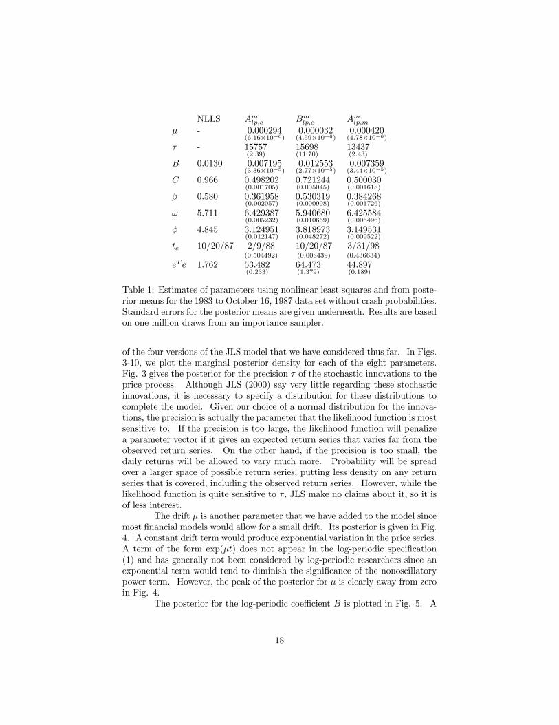
Table 1: Estimates of parameters using nonlinear least squares and from poste-rior means for the 1983 to October 16, 1987 data set without crash probabilities.Standard errors for the posterior means are given underneath. Results are basedon one million draws from an importance sampler.
of the four versions of the JLS model that we have considered thus far. In Figs.3-10, we plot the marginal posterior density for each of the eight parameters.Fig. 3 gives the posterior for the precision τ of the stochastic innovations to theprice process. Although JLS (2000) say very little regarding these stochasticinnovations, it is necessary to specify a distribution for these distributions tocomplete the model. Given our choice of a normal distribution for the innova-tions, the precision is actually the parameter that the likelihood function is mostsensitive to. If the precision is too large, the likelihood function will penalizea parameter vector if it gives an expected return series that varies far from theobserved return series. On the other hand, if the precision is too small, thedaily returns will be allowed to vary much more. Probability will be spreadover a larger space of possible return series, putting less density on any returnseries that is covered, including the observed return series. However, while thelikelihood function is quite sensitive to τ , JLS make no claims about it, so it isof less interest.
The drift µ is another parameter that we have added to the model sincemost financial models would allow for a small drift. Its posterior is given in Fig.4. A constant drift term would produce exponential variation in the price series.A term of the form exp(µt) does not appear in the log-periodic specification(1) and has generally not been considered by log-periodic researchers since anexponential term would tend to diminish the significance of the nonoscillatorypower term. However, the peak of the posterior for µ is clearly away from zeroin Fig. 4.
The posterior for the log-periodic coefficient B is plotted in Fig. 5. A
18
Figure 3: Posterior density for the precision τ in the market-time model withdiffuse priors and no crash probabilities (Anclp,m).
Figure 4: Posterior density for the drift µ in the market-time model with diffusepriors and no crash probabilities (Anclp,m).
19
Figure 5: Posterior density for the log of the log-periodic coefficient lnB in themarket-time model with diffuse priors and no crash probabilities (Anclp,m).
classical approach to testing the log-periodic hypothesis would be to test thenull hypothesis that B = 0. One might think that a natural analog to this inthe Bayesian paradigm would be to look at whether the posterior for B peaksat zero. However, the prior density for B at B = 0 is zero. That is why wehave to consider the null hypothesis where B = 0 as the separate model Ancn,m.The graph does show though that lnB peaks about -5 with B ∼ 0.007, which isroughly the posterior mean. This is smaller than the NLLS estimate of 0.13.10
We did not plot the corresponding priors in the above graphs of theprecision, drift, and log-periodic coefficient because the data must necessarilybe informative about the values of these three parameters. In the remaininggraphs, we also give the prior for comparison. If B = 0, the likelihood functionwill not depend on β, tc, ω, C, or φ. In that case, the remaining five parameterswould not be identified by the model, so estimating them would be pointless.Since the posterior for B is concentrated around small values, it may still be thecase that the likelihood function is practically independent of these parameters,in which case the posterior and prior densities will be the same, and we canview these parameters as “spurious”.
Both the posterior and prior densities for the exponent β are givenin Fig. 6. Clearly, the data are informative about β since the posterior ismonotonically decreasing whereas the uniform prior is flat. In this case, theposterior mean of 0.38 understates how bad the NLLS estimate of β = 0.58 is
10Strictly speaking, we should be comparing the market-time model to NLLS estimatesfrom the market-time model. However, there is not much difference between the posteriorsfor the market and calendar-time models with diffuse priors.
20
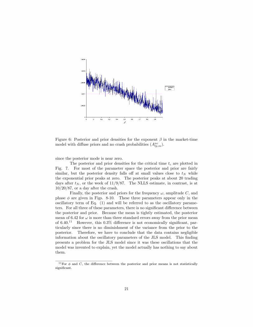
Figure 6: Posterior and prior densities for the exponent β in the market-timemodel with diffuse priors and no crash probabilities (Anclp,m).
since the posterior mode is near zero.The posterior and prior densities for the critical time tc are plotted in
Fig. 7. For most of the parameter space the posterior and prior are fairlysimilar, but the posterior density falls off at small values close to tN whilethe exponential prior peaks at zero. The posterior peaks at about 20 tradingdays after tN , or the week of 11/9/87. The NLLS estimate, in contrast, is at10/20/87, or a day after the crash.
Finally, the posterior and priors for the frequency ω, amplitude C, andphase φ are given in Figs. 8-10. These three parameters appear only in theoscillatory term of Eq. (1) and will be referred to as the oscillatory parame-ters. For all three of these parameters, there is no significant difference betweenthe posterior and prior. Because the mean is tightly estimated, the posteriormean of 6.42 for ω is more than three standard errors away from the prior meanof 6.40.11 However, this 0.3% difference is not economically significant, par-ticularly since there is no diminishment of the variance from the prior to theposterior. Therefore, we have to conclude that the data contains negligibleinformation about the oscillatory parameters of the JLS model. This findingpresents a problem for the JLS model since it was these oscillations that themodel was invented to explain, yet the model actually has nothing to say aboutthem.
11For φ and C, the difference between the posterior and prior means is not statisticallysignificant.
21
Figure 7: Posterior and prior densities for the critical time tc in the market-timemodel with diffuse priors and no crash probabilities (Anclp,m).
Figure 8: Posterior and prior densities for the frequency ω in the market-timemodel with diffuse priors and no crash probabilities (Anclp,m).
22
Figure 9: Posterior and prior densities for the amplitude C in the market-timemodel with diffuse priors and no crash probabilities (Anclp,m).
Figure 10: Posterior and prior densities for the phase φ in the market-timemodel with diffuse priors and no crash probabilities (Anclp,m).
23
Figure 11: Posterior density for the precision τ in the calendar-time model withtight priors and no crash probabilities (Bnclp,c).
5.2 Posterior Graphs for Calendar-TimeModel with TightPriors
The calendar-time model with tight priors is the model that would mostresemble what has been discussed in the previous literature, so we also plot themarginal posterior densities for its parameters. These are shown in Figs. 11-18. Unlike with diffuse priors, the posteriors for all the log-periodic parameters,including the oscillatory parameters, differ significantly from the priors.
The tight priors for the exponent β and the critical time tc both have asingle, roughly symmetric peak away from zero, so they are markedly differentfrom the corresponding diffuse priors. Consequently, the posteriors for theseparameters are also quite different from the corresponding posteriors with dif-fuse priors. In Figs. 14-15, both parameters exhibit posteriors with roughlysymmetric peaks like the prior. Consistent with the difference between the priorand posterior means for β reported in Table 1, the posterior mode for β is lowerthan the prior mode, confirming that the model favors lower values of β thanwould be obtained with NLLS curve fitting. This is also true for tc althoughthe difference in the prior and posterior modes is less than a day. Note that inboth cases the posterior mode cannot move too far away from the prior modesince if the prior puts zero weight on a parameter vector the posterior must dothe same.
Fig. 16 demonstrates that the posterior for the frequency ω has at leastthree peaks. As is shown in Fig. 17, the posterior for the amplitude C is notuniform like for the diffuse prior, but is weighted toward the maximum valueof 1. Keeping in mind that the posterior for the phase φ has to wrap around
24
Figure 12: Posterior density for the drift µ in the calendar-time model withtight priors and no crash probabilities (Bnclp,c).
Figure 13: Posterior density for the log of the log-periodic coefficient lnB in thecalendar-time model with tight priors and no crash probabilities (Bnclp,c).
25
Figure 14: Posterior and prior densities for the exponent β in the calendar-timemodel with tight priors and no crash probabilities (Bnclp,c).
Figure 15: Posterior and prior densities for the critical time tc in the calendar-time model with tight priors and no crash probabilities (Bnclp,c).
26
Figure 16: Posterior and prior densities for the frequency ω in the calendar-timemodel with tight priors and no crash probabilities (Bnclp,c).
continuously from 2π back to 0, we see in Fig. 18 that the φ posterior has a singlepeak between 3π/2 and 2π. These results suggest that the likelihood functionis not, in fact, completely insensitive to the oscillatory parameters. Tighteningthe prior allows us to probe the likelihood function at a smaller scale, and thisreveals that there is structure to the likelihood function along the oscillatorydimensions.
However, if we do not have a reason to believe that the parameters ofa model are most likely to fall in a given region, it does not make sense toconcentrate the probability density of our prior within that region. We choseour tight prior based on NLLS curve fitting, but, as we have seen, tightening theprior in this way actually diminishes the marginal likelihood, suggesting thatthe most likely parameter values are not close to their NLLS estimates. Thisinterpretation is also supported by the above findings regarding tc and β. Inthe next section, we will see further evidence of this in the posterior distributionof the residuals sum minimized by the NLLS procedure.
6 Nonlinear Least Squares
In addition to computing the posterior distribution for the parameters ofa model, the Bayesian paradigm allows us to compute posterior distributionsfor any function of the parameters, including the sum of the squared residualsbetween the raw financial time series and the model’s prediction for the time
27
Figure 17: Posterior and prior densities for the log-periodic amplitude C in thecalendar-time model with tight priors and no crash probabilities (Bnclp,c).
Figure 18: Posterior and prior densities for the phase φ in the calendar-timemodel with tight priors and no crash probabilities (Bnclp,c).
28
series. According to the JLS model, the expectation of the log price at time tiis
E[qti ] = qt0 + µ(ti − t0) +∆H(ti, t0). (10)
If we define
ei = qti −E[qti ] i = 0, . . . ,m,
then the NLLS procedure, which has generally been followed in the existingliterature, is to choose the parameters ξ that minimize
eT e =NXi=0
e2i .
Note that the specification of Eq. (10) differs from the standard log-periodic specification of (1) in two respects. First, as we have noted before, wehave included a linear drift term in (10), which generally is not done. Second,and more important, the constant term in (10) is the log of the price at theinitial time t0. In contrast, the constant term in (1) is a free parameter thatis also determined by the fitting procedure. Since the linear term in (10) ispartially correlated with the non-oscillatory component of the ∆H term, addingthe linear term cannot help in minimizing eT e as much as varying the constantwill. As a result, even if we augment the JLS model by adding the linear termto E[qti ], it is not possible to get values of e
T e as low as one would get by usingNLLS to estimate A and ξ in the standard specification of (1).
For example, in the context of the calendar-time model, the smallestvalue of eT e obtained by our importance sampler was 2.72. This was obtainedwith the parameters µ = −0.0003, B = 0.00964, C = 0.769, β = 0.675, ω =11.589, φ = 6.259, and tc = 10/20/87. The corresponding fit used to determinethe tight priors in Section 4 had a much smaller eT e of 1.76. However, if weadjust the constant A in that fit from 5.918 to 5.711 so that E[qt0 ] = qt0 , thenthe residual sum increases to 9.12.
The posterior densities for eT e in the market-time model with diffusepriors and in the calendar-time model with tight priors are respectively givenin Figs. 19 and 20. In both cases, most of the density is concentrated aroundsmall values of eT e. However, the density is not maximized at the minimumpossible value of eT e. For the calendar-time model, the posterior is maximizedat eT e = 6.25, which is small but twice as large as the minimum observed valueof 2.72. A similar story can be told regarding the market-time model.
Thus, the most likely value of eT e in the JLS model is not the minimumpossible value, and it is easy to see why. The justification for least-squares min-imiziation, when it is appropriate, is that the likelihood function is a decreasingfunction of eT e, as would happen for example if we were estimating a model ofthe form
yj =mXi=1
aixij + εj , (11)
29
Figure 19: Posterior density for the nonlinear least squares residuals sum eT ein the market-time model with diffuse priors and no crash probabilities (Anclp,m).
Figure 20: Posterior density for the nonlinear least squares residuals sum eT ein the calendar-time model with tight priors and no crash probabilities (Bnclp,c).
30
based on J observations of combinations of a dependent variable y and m in-dependent variables x1, . . . , xm. If the disturbance term εj is normallydistributed, then the likelihood function will depend only on the sum of theresiduals for this model and the variance of the εj .
As was done in Feigenbaum (2001a), one can estimate the JLS modelin this matter, but it is the daily returns qti − qti−1 that behave as a (nonlinear)model similar to (11), not the qti themselves. Consequently, the likelihoodfunction is, modulo an irrelevant constant,
L = N
2ln τ − τ
2S2,
where
S2 =NXi=1
¡qti − qti−1 −E[qti − qti−1 ]
¢2ti − ti−1
=NXi=1
¡qti − qti−1 − µ(ti − ti−1)−∆H(ti, ti−1)
¢2ti − ti−1
.
Thus the likelihood function will be maximized with respect to µ and ξ if S2
is minimized. While it is true that eT e and S2 are highly correlated, it is nottrue that the global minimum of S2 corresponds to the global minimum of eT e.Indeed, for the calendar-time model with tight priors, the draw with the highestobserved posterior density12 had S2 = 0.0769 and eT e = 5.25 while the drawwith the minimum value of eT e = 2.72 had S2 = 0.0778.
In the language of econometrics, NLLS estimation of the specification(1) does not consistently estimate the parameters of the JLS model. As Feigen-baum (2001a) argued, in order to determine the parameters of the JLS modelone needs to focus on the daily returns and not the raw price time series. TheJLS model defines a stochastic process for the daily returns, and the prices areobtained by integrating those returns. The literature has generally proceededin the reverse fashion, by regressing a model of the prices and obtaining returnsby differencing the prices, and this backwards approach is not appropriate formodel estimation.
7 Model with Crash Probabilities
Thus far, we have considered a model in which daily returns vary log-periodically, but we have ignored the reason why they vary log-periodically in theJLS model, which is that the probability of a crash also varies log-periodically.Classical curve-fitting and spectral methods are unable to take into account this
12The parameters of this highest posterior draw were µ = 9.87×10⁻⁵, τ = 15323, B = 0.013,C = 0.94, β = 0.55, ω = 5.70, φ = 4.96, and tc = 10/20/87.
31
time-varying crash probability, so the existing literature has been dominated bydiscussion of an incomplete model.13 This is of concern because, if the modelpredicts that the probability of a crash on 10/19/87 is on the order of 10−5, thisprobability is smaller than the empirical frequency of crashes and the modelwould not do a very good job of explaining crashes. On the other hand, if themodel predicts that the probability of a crash on any day between 1983 and1987 was on the order of 10%, the model would run into the opposite problembecause the crash should have occurred much sooner than 10/19/87.
With Bayesian methods, it is straightforward to complete the model byadding in the crash probabilities, and this is what we will do in this section.To do this we must first specify the distribution of crash sizes. We only havethe one crash event in our 1980 to 1987 data set, so we will assume a dogmatic,degenerate distribution for the crash size κ. The S&P 500 fell from 282.70 to224.84 on 10/19/87, which translates to a fall of 0.22900 in the logarithm q.Thus, we will assume that κ = 0.22900 with probability 1.
From Eq. (4), conditional upon a crash not occurring at the prior timest1, . . . , ti−1 a crash will occur at ti ≥ t1 with the probability
1− expµ−∆H(ti−1, ti)
κ
¶.
Thus, the posterior density inclusive of the crash probabilities is
pclp(θ|QtN+1
t0 ) = pnc(θ|QtN+1
t0 ) exp
Ã−
NXi=1
∆H(ti−1, ti; ξ)
κ
!(12)
×µ1− exp
µ−∆H(tN ,min{tN+1, tc}; ξ)
κ
¶¶.
Note that in the last factor, the probability that a crash happens between tNand tN+1 = 10/19/87, we integrate the hazard rate from tN to either tN+1 or tc,whichever is smaller. Once tc is reached, if the crash has not occurred already,it will not occur. What happens after tc is not specified by the JLS model.
As a null hypothesis, we will construct an alternative model with aconstant probability of a crash of magnitude κ on any given trading day.14
From 1962 to 1998, there were 9190 trading days, and there were no other dayswhen the market dropped as much as it did on 10/19/87. Thus, we will assumea constant probability of pcr = 1/9190 for the market to drop by κ on any giventrading day. Given that a crash did not occur on the initial day in our dataset, 1/3/83, there were N = 1211 days between 1/3/83 and 10/16/87 on which
13Note that there are classical methods that can take into account the crash probabilities.Maximum likelihood estimation (MLE) of the JLS model could incorporate the crash proba-bilities into the likelihood function as we have done, but, to our knowledge, no researcher hasused MLE to estimate the model.14If daily returns are normally distributed, the standard deviation would have to be on the
order of 1% to fit most price data, in which case the probability of the market dropping by asmuch as 20% on any given day would be astronomically small. So we must introduce anothermechanism to plausibly account for crashes in the null hypothesis.
32
a crash again did not occur, and then there was one day in which a crash didoccur. Thus, under the null hypothesis the posterior density inclusive of thecrash probabilities is
pcn(θ|QtN+1
t0 ) = pnc(θ|QtN+1
t0 )(1− pcr)Npcr.
Taking into account the crash probabilities, we find the following mar-ginal likelihoods with 1,000,000 draws:
Lc³Acn,c|Q
10/16/871/3/83
´= 3971.3871± 0.0428
Lc³Aclp,c|Q
10/16/871/3/83
´= 3971.9977± 0.1369
Lc³Acn,m|Q
10/16/871/3/83
´= 4019.7889± 0.0405
Lc³Aclp,m|Q
10/16/871/3/83
´= 4020.4599± 0.0654
Lc³Bcn,c|Q
10/16/871/3/83
´= 3973.6069± 0.0144
Lc³Bclp,c|Q
10/16/871/3/83
´= 3970.6058± 0.0814
Lc³Bcn,m|Q
10/16/871/3/83
´= 4021.8448± 0.0145
Lc³Bclp,m|Q
10/16/871/3/83
´= 4019.8423± 0.0439.
In the complete model, with tight priors the null hypothesis still wins outover the JLS model in terms of marginal likelihood. On the other hand, withdiffuse priors the JLS model now outperforms the null hypothesis. So, onceagain, we find that the parameter estimates obtained by least-squares estimationare not very probable under the JLS model.
The reversal of marginal likelihoods for the diffuse-prior models is notentirely surprising since, without crash probabilities, the marginal likelihood ofthe null hypothesis models was only slightly higher than for the JLS models.The JLS model has an explicit explanation why a crash should happen on oraround 10/19/87 while the null hypothesis does not. Accounting for the crashprobabilities should benefit the JLS model relative to the null hypothesis, andwith the diffuse priors it does so enough to push the balance in favor of the JLSmodel. With market timing, adding crashes increases the Bayes factor for theJLS model relative to the null hypothesis from 0.75 to 1.96.
However, the better performance of the JLS model with diffuse pri-ors at explaining crashes does not translate to better performance at explain-ing log-periodic oscillations. The posterior means for the diffuse-prior modelsand for the tight-prior model with calendar timing are reported in Table 2.The posterior densities for the parameters, as well as the residuals sum eT e, ofthe market-timing model with diffuse priors are plotted in Figs. 21-29. Theonly parameters that exhibit a major change are the log-periodic coefficient B,
33
NLLS Aclp,c Bclp,c Aclp,mµ - 0.000345
(7.74×10⁻¹⁰)0.000122(4.14×10⁻⁶)
0.000484(1.22×10⁻⁶)
τ - 15747(2.49)
15687(13.07)
13434(2.36)
B 0.0130 0.009917(4.80×10⁻⁵)
0.012525(2.48×10⁻⁵)
0.009632(5.11×10⁻⁵)
C 0.966 0.497774(0.001420)
0.703691(0.005681)
0.490394(0.001662)
β 0.580 0.336835(0.001031)
0.493638(0.000957)
0.386423(0.001132)
ω 5.711 6.409146(0.005892)
5.988231(0.014062)
6.426282(0.006706)
φ 4.845 3.124951(0.012147)
3.662840(0.057786)
3.138914(0.010267)
tc 10/20/87 12/17/87(0.504492)
10/20/87(0.010463)
1/27/88(0.364815)
eT e 1.762 53.178(0.202)
60.357(1.378)
45.19711(0.190)
Table 2: Estimates of parameters using nonlinear least squares and from poste-rior means for the 1983 to October 16, 1987 data set with crash probabilities.Standard errors for the posterior means are given underneath. Results are basedon one million draws from an importance sampler.
the power β, and the critical time tc. There was no reason to expect thatadding crash probabilities would significantly change the posterior probabilitiesfor the oscillatory parameters, and Figs. 26-28 confirm that the posteriors forthese parameters remain essentially unchanged from their priors in the completemodel.15
What distinguishes B, β, and tc is that these are the three parametersthat play the largest role in determining how the crash probability behavesover time. Since the crash probability at ti is approximately proportional to∆H(ti, ti−1), and ∆H is proportional to B, a higher B means a higher crashprobability, and the posterior mean for B increases from .0073 to .0096 whenwe add crash probabilities. We can also see the shift to higher values of B bycomparing Fig. 5 to Fig. 23.
Meanwhile, if we ignore the oscillatory term, the crash probability willgo roughly as
Since a crash did not occur between 1/1/83 and 10/16/87 and a crash did occuron 10/19/87, the likelihood function should favor a choice of β and tc thatconfers a low probability of a crash for most of the 1983 to 1987 and then hasthe probability shoot up just prior to 10/19/87. This can be achieved by havingβ ≈ 0 and tc ≈ 10/19/87. Comparing Figs. 7 and 25, we find in the completemodel that the posterior for low tc is higher than the prior, in contrast to the
15The posterior for ω in Fig. 26 does exhibit one abnormally high point, but this is stillwithin two standard errors of the prior.
34
Figure 21: Posterior density for the precision τ in the market-time model withdiffuse priors and crash probabilities (Aclp,m).
Figure 22: Posterior density for the drift µ in the market-time model with diffusepriors and crash probabilities (Aclp,m).
35
Figure 23: Posterior for the log of the log-periodic coefficient lnB in the market-time model with diffuse priors and crash probabilities (Aclp,m).
Figure 24: Posterior and prior density for the exponent β in the market-timemodel with diffuse priors and crash probabilities (Aclp,m).
36
Figure 25: The posterior and prior densities for the critical time tc in the market-time model with diffuse priors and crash probabilities (Aclp,m).
Figure 26: Posterior and prior densities for the frequency ω in the market-timemodel with diffuse priors and crash probabilities (Aclp,m).
37
Figure 27: Posterior and prior densities for the amplitude C in the market-timemodel with diffuse priors and crash probabilities (Aclp,m).
Figure 28: Posterior and prior density for the phase φ in the market-time modelwith diffuse priors and crash probabilities (Aclp,m).
38
Figure 29: Posterior density for the nonlinear least squares residuals sum eT ein the market-time model with diffuse priors and crash probabilities (Aclp,m).
model without crash probabilities. In Fig. 24, meanwhile, we see that there isnow a small secondary peak at low values of β. Counterintuitively, the posteriormode and mean for β are pushed to higher values in the complete model, whichprobably happens because, for high values of tc, a large β is needed to get thecrash probability to increase significantly as t approaches 10/19/87.
On a side note, since the likelihood function will put even less priorityon fitting the raw price data in the complete model than it did without crashprobabilities, one would expect to get larger values of the residuals sum eT e.However, we do not find a statistically significant difference between the means,and the posterior density of Fig. 29 is little changed from the correspondinggraph of Fig. 19 for the model without crash probabilities.
Incorporating crash probabilities of the JLS model into our analysisdoes not do much, good or bad, to the model’s ability to explain log-periodicoscillations, although it does show that the model can outperform a model witha constant crash probability in terms of explaining when crashes occur.
8 Conclusion
Let us suppose that the log-periodic hypothesis is, indeed, correct. Esti-mation of the parameters of Eq. (1) by direct NLLS curve fitting of a raw priceseries to the log-periodic specification produces descriptive statistics that char-acterize any log-periodic oscillations that occur in a given time window. As we
39
have seen, though, such descriptive statistics may not translate to the parame-ters of the underlying model responsible for those oscillations. For researchersinterested in modeling financial markets as complex systems, it is ultimatelythose fundamental model parameters that are of interest, not the descriptivestatistics.
Previous attempts to estimate the parameters of the Johansen-Ledoit-Sornette (2001) model of log-periodicity have been hampered by technical issues.Here, we have skirted those issues by employing Bayesian methods, which arebetter suited for the analysis of complicated time-series models like the JLSmodel. However, our findings do not provide support for the claim that theJLS model can explain log-periodic oscillations. In examining the period pre-ceding the stock market crash of October 1987, we find that the complete modeloutperforms a null hypothesis model in terms of explaining why a crash wouldoccur on 10/19/87, yet the data set is uninformative about the oscillatory pa-rameters of the model. This suggests that those oscillatory parameters play noactual role.
The scope of our analysis was limited because we only considered datafrom a single log-periodic spell. One argument in favor of the log-periodichypothesis is that similar values of the frequency ω are observed throughoutthe set of known log-periodic precursors. If one generalized the JLS model sothat it described the behavior of financial markets both during periods of log-periodicity and during more quiescent periods, one could use the entire historyof financial prices to obtain a posterior for the distribution from which ω isdrawn for each log-periodic spell. If the value of ω is truly a universal propertyof log-periodic spells, the set of all log-periodic spells should be more informativeabout the oscillatory parameters of the JLS model than one log-periodic spellin isolation. Such a global analysis might then provide more support for theJLS model than could be found in the short data set considered here.
Even so, a negative result for the JLS model should not be interpretedas a negative result for the log-periodic hypothesis as a whole. The head andshoulders phenomenon, long recognized by technical traders, is another patternin stock prices that has recently been found to predict excess returns over timescales of a month or longer (Savin, Weller, and Zvingelis (2003)). So it isnot unreasonable to think that a pattern like log-periodicity might also havepredictive power, but a different approach may be needed to explain how thishappens.
In the JLS model, log-periodicity in financial prices reflects log-periodic-ity in traders’ expectations regarding the future path of those prices. Anothermodel of this class is pursued by Sornette and Ide (2003). They constructa deterministic model in which log-periodicity results from the interaction offundamental and technical traders. Since the real world is not deterministic,Sornette and Ide presumably have in mind that actual prices dance aroundan expected price path that behaves as in their model. For both models,if the expected price path is log-periodic, then expected daily returns shouldalso behave log-periodically, yet we find no evidence of such log-periodicity inreturns.
40
This suggests that researchers should look to other explanations of log-periodicity that do not involve expectations. For example, Stauffer and Sornette(1998) constructed a model where prices are governed by a biased diffusionprocess that produces log-periodic behavior. They offered no microfoundationsfor why the market should behave in this way, but one could presumably explainthis behavior in terms of, possibly psychological, barriers. If the market hasa tendency to reverse direction when prices hit a floor or ceiling, log-periodicoscillations would occur if prices go back and forth between the two barriersat an increasing rate. One could then imagine that an acceleration in therate of hitting barriers might make the market more susceptible to a crash.This approach would not share the JLS model’s consistency with the EfficientMarkets Hypothesis, but the mainstream finance literature is starting to becomemore receptive to behavioral models that deviate from rationality (Barberis andThaler (2002)).
A The Hazard Rate
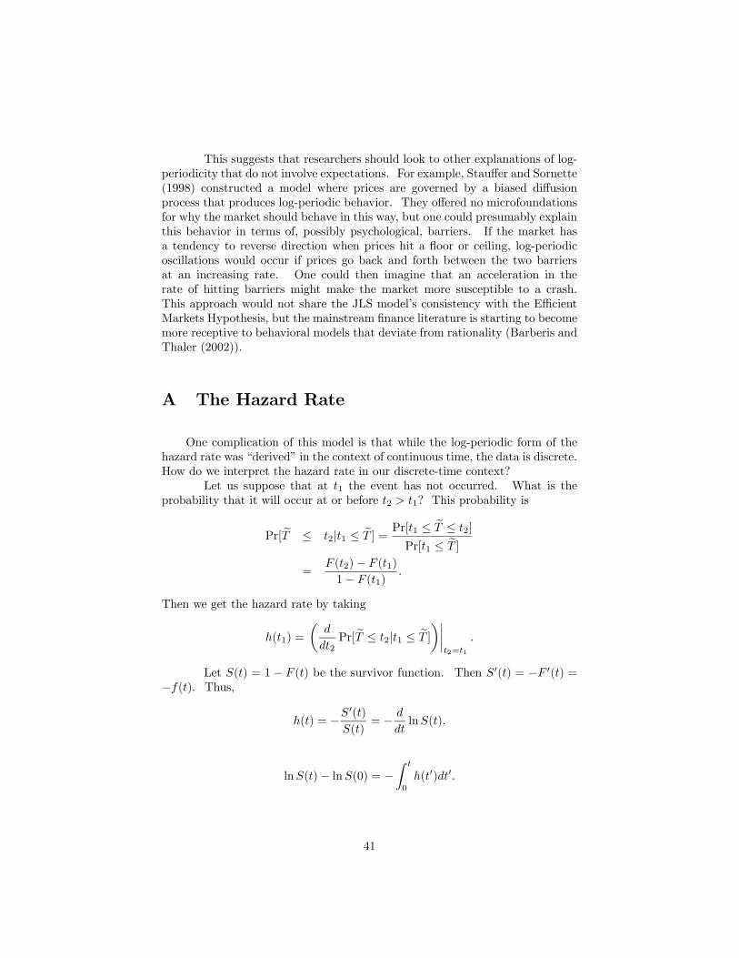
One complication of this model is that while the log-periodic form of thehazard rate was “derived” in the context of continuous time, the data is discrete.How do we interpret the hazard rate in our discrete-time context?
Let us suppose that at t1 the event has not occurred. What is theprobability that it will occur at or before t2 > t1? This probability is
Pr[eT ≤ t2|t1 ≤ eT ] = Pr[t1 ≤ eT ≤ t2]Pr[t1 ≤ eT ]
=F (t2)− F (t1)1− F (t1)
.
Then we get the hazard rate by taking
h(t1) =
µd
dt2Pr[eT ≤ t2|t1 ≤ eT ]¶¯̄̄̄
t2=t1
.
Let S(t) = 1− F (t) be the survivor function. Then S0(t) = −F 0(t) =−f(t). Thus,
h(t) = −S0(t)
S(t)= − d
dtlnS(t).
lnS(t)− lnS(0) = −Z t
0
h(t0)dt0.
41
Since S(0) = 1,
S(t) = exp
µ−Z t
0
h(t0)dt0¶.
Then
Pr[eT ≤ t2|t1 ≤ eT ] = S(t1)− S(t2)S(t1)
=exp
³−R t10h(t0)dt0
´− exp
³−R t20h(t0)dt0
´exp
³−R t10h(t0)dt0
´Thus,
Pr[eT ≤ t2|t1 ≤ eT ] = 1− expµ−Z t2
t1
h(t0)dt0¶. (13)
In the limit of smallR t2t1h(t0)dt0,
Pr[eT ≤ t2|t1 ≤ eT ] ≈ Z t2
t1
h(t0)dt0, (14)
which is what people usually say the conditional probability will be. However,(13) is the exact probability, and it will always be between 0 and 1, unlike theapproximate result (14).
B Properties of the Hazard Rate
An important property of the hazard rate function is that its integral willhave the same form as itself, a power law times a periodic function of ln(tc − t)with frequency ω. This is because
h(t) = RehB(tc − t)1−α
n1 + Ceiφ
0(tc − t)iω
oi,
and the derivative or integral of a power law is also a power law (assuming theexponent is not -1). Focusing on a strictly real representation of h, consider afunction
If we set γ = α, F 01 = −B0, F 02 = C, and F 03 = 0, then h(t) has the form of Eq.(16) Therefore, the integral of the hazard rate has the form of (15) up to aconstant, so
⎡⎢⎢⎣1 + C cos θ cos(ω ln(tc − t) + φ0) + sin θ sin(ω ln(tc − t) + φ0)r1 +
³ω1−α
´2⎤⎥⎥⎦
= A−B(tc − t)1−α
⎡⎢⎢⎣1 + Cr1 +
³ω1−α
´2 cos(ω ln(tc − t) + φ)
⎤⎥⎥⎦ ,where B = κB0/(1− α) and φ = φ0 − θ.
C Importance Sampling
Denote the target density by p(θ). Denote the source density by j(θ), andan arbitrary kernel of the source density kj (θ) = cj ·j(θ) for any cj 6= 0. Denotean arbitrary kernel of the target density by kp (θ) = cp · p(θ) for any cp 6= 0.The following result is due to Geweke (1989). Suppose that the sequencenθ(m)
oMm=1
is independent and identically distributed, with θ(m) ∼ j(θ). Define
the weighting function w(θ) =kp(θ)kj(θ)
. Suppose E [g(θ)] exists, E[w(θ)] exists,
and the support of j(θ) include Θ. Then
g(M) =
MPm=1
g(θ(m))w(θ(m))
MPm=1
w(θ(m))
→ E [g(θ)]
Assuming V [g(θ)] exists, then
M1/2(g(M) −E[g(θ)]) d→ N(0, τ2),
where
bτ2(M) =MPM
m=1
hg(θ(m))− g(M)
i2w(θ(m))2µ
MPm=1
w(θ(m))
¶2 a.s.→ τ2.
44
References
[1] Barberis, Nicholas and Richard Thaler, (2002), “A Survey of BehavioralFinance,” forthcoming in the Handbook of the Economics of Finance.
[2] Berger, J. O., (1985), Statistical Decision Theory and Bayesian Analysis(Springer-Verlag: New York).
[3] Bernardo, J. M. and A. F. M. Smith, (1994), Bayesian Theory (Wiley:New York).
[4] Blanchard, Olivier Jean and Stanley Fischer, (1989), Lectures on Macroe-conomics (MIT Press, Cambridge).
[5] Fama, Eugene F., (1970), “Efficient Capital Markets: A Review of Theoryand Empirical Work,” Journal of Finance 25: 383-417.
[6] Feigenbaum, James, (2001), “A Statistical Analysis of Log-Periodic Pre-cursors to Financial Crashes,” Quantitative Finance 1: 346.
[7] Feigenbaum, James, (2001), “More on A Statistical Analysis of Log-Periodic Precursors to Financial Crashes,” Quantitative Finance 1: 527-532.
[8] Feigenbaum, James (2003), “Financial Physics,” Reports on Progress inPhysics 66: 1611-1649.
[9] Feigenbaum, James and Peter G. O. Freund, (1996), “Discrete Scale Invari-ance in Stock Markets Before Crashes,” International Journal of ModernPhysics B 10: 3737-3745.
[10] Gelman, A., J. Carlin, H. Stern, and D. Rubin, (2003), Bayesian DataAnalysis (Chapman & Hall: Boca Raton).
[11] Geweke, John, (1989), “Bayesian Inference in Econometric Models UsingMonte Carlo Integration,” Econometrica 57: 1317-1340.
[12] Graf v. Bothmer, Hans-Christian and Christian Meister, (2003), “Predict-ing Critical Crashes? A New Restriction for Free Variables,” Physica A 320:539-547.
[13] Ilinski, Kirill, (1999), “Critical Crashes?,” International Journal of ModernPhysics C 10: 741-746.
[14] Johansen, Anders, (2004), “Origin of Crashes in Three US Stock Markets:Shocks and Bubbles,” Physica A 338: 135-142.
[15] Johansen, Anders, Olivier Ledoit, and Didier Sornette, (2000), “Crashes asCritical Points,” International Journal of Theoretical and Applied Finance3: 219-255.
45
[16] Johansen, A., D. Sornette, G. Wakita, U. Tsunogai, W. I. Newman, andH. Saleur, (1996), “Discrete Scaling in Earthquake Precursory Phenomena:Evidence in the Kobe Eartquake, Japan,” J. Phys. I. (France) 6: 1391-1402.
[18] Laloux, L., M. Potters, J. P. Aguilar, and J. P. Bouchaud, (2002), “Replyto Johansen’s Comment,” Europhysics Letters 45: 1.
[19] Phillips, P. C. B., (1986), “Understanding Spurious Regressions in Econo-metrics,” Journal of Econometrics 33: 311-340.
[20] Savin, Gene, Paul Weller, and Janis Zvingelis, (2003), “The PredictivePower of Head-and-Shoulders Price Patterns in the U.S. Stock Market,”Working Paper.
[22] Sornette, Didier, (2003), Why Stock Markets Crash: Critical Events inComplex Financial Systems (Princeton University Press: Princeton, NJ).
[23] Sornette, Didier and Kayo Ide, (2003), “Theory of Self-Similar OscillatoryFinite-Time Singularities in Finance, Population and Rupture,” Interna-tional Journal of Modern Physics C 14: 267-275.
[24] Sornette, Didier, Anders Johansen, and Jean-Phillipe Bouchaud, (1996),“Stock Market Crashes, Precursors and Replicas,” J. Phys. I. (France) 6:167-175.
[25] Stauffer, Dietrich and Didier Sornette, (1998), “Log-Periodic Oscillationsfor Biased Diffusion on Random Lattice,” Physica A 252: 271-277.
[26] Sornette, Didier and Wei-Xing Zhou, (2003), “Predictability of Large Fu-ture Changes in Complex Systems,” cond-mat/0304601.