Engineering Structures 29 (2007) 1548–1560 www.elsevier.com/locate/engstruct A bidirectional and homogeneous tuned mass damper: A new device for passive control of vibrations Jos´ e L. Almaz´ an, Juan C. De la Llera, Jos´ e A. Inaudi, Diego L´ opez-Garc´ ıa * , Luis E. Izquierdo Departamento de Ingenier´ ıa Estructural y Geot´ ecnica, Pontificia Universidad Cat´ olica de Chile, Macul, Santiago 690441, Chile Received 12 March 2006; received in revised form 4 September 2006; accepted 7 September 2006 Available online 23 October 2006 Abstract Passive tuned-mass dampers (TMDs) are a very efficient solution for the control of vibrations in structures subjected to long-duration, narrow- band excitations. In this study, a Bidirectional and Homogeneous Tuned Mass Damper (BH-TMD) is proposed. The pendular mass is supported by cables and linked to a unidirectional friction damper with its axis perpendicular to the direction of motion. Some advantages of the proposed BH-TMD are: (1) its bidirectional nature that allows control of vibrations in both principal directions; (2) the capacity to tune the device in each principal direction independently; (3) its energy dissipation capacity that is proportional to the square of the displacement amplitude, (4) its low maintenance cost. Numerical results show that, under either unidirectional or bidirectional seismic excitations, the level of response reduction achieved by the proposed BH-TMD is similar to that obtained from an “ideal” linear viscous device. Moreover, experimental shaking table tests performed using a scaled BH-TMD model confirm that the proposed device is homogeneous, and, hence, its equivalent oscillation period and damping ratio are independent of the motion amplitude. c 2006 Elsevier Ltd. All rights reserved. Keywords: Tuned mass damper; Passive control; Structural dynamics; Bi-directional control; Homogeneous device; Frictional damping; Low-cost TMD implementation 1. Introduction Passive Tuned Mass Dampers (TMDs) are used in vibration reduction of flexible structures subjected to long-duration narrow-band excitations [1–3]. While a TMD does not necessarily reduce the peak deformation demand in an inelastic structure subjected to ground motion, it reduces the corresponding level of damage [5,6]. In the TMD literature, there are publications that deal with the bidirectional behavior of a structure. Most of this research aims to control the lateral–torsional response of the bare structure by means of multiple unidirectional TMDs [7, 8]. In order to use the total weight of the supplemental mass, a typical design would consider one or multiple bidirectional TMDs, with frequencies tuned independently in each principal * Corresponding address: Departamento de Ingenier´ ıa Estructural y Geot´ ecnica, Pontificia Universidad Cat´ olica de Chile, Av. Vicuna Mackenna 4860, 782-0436 Santiago, RM, Chile. Tel.: +56 2 354 7684; fax: +56 2 354 4243. E-mail address: [email protected](D. L ´ opez-Garc´ ıa). direction of the structure. As far as the authors know, the behavior of nominally symmetric structures with TMDs subjected to bidirectional excitations has not been considered in the literature. Since the implementation of TMDs is often restricted by budget and technical constraints, it is important to devise a low cost TMD solution that is simple, robust, and of simple installation and maintenance. Motivated by that, a novel device whose design is intended to overcome the aforementioned constraints is presented in this paper. One of its innovative features is the structural layout in which the mass is attached to the main structure, a simple implementation that makes the tuning process of the device easy and inexpensive, and allows the device to be tuned independently in each principal direction. Another innovative feature of the proposed device is the use of a friction damper instead of a viscous damper, attached to the TMD mass in a direction perpendicular to the plane of motion of the mass. This approach follows the idea presented earlier by Inaudi and Kelly [9] that results in energy dissipation quadratic in amplitude, and hence, an equivalent damping ratio independent of the motion amplitude. This is in contrast to 0141-0296/$ - see front matter c 2006 Elsevier Ltd. All rights reserved. doi:10.1016/j.engstruct.2006.09.005
Passive Tuned Mass Dampers (TMDs) are used in vibrationreduction of flexible structures subjected to long-durationnarrow-band excitations [1–3]. While a TMD does notnecessarily reduce the peak deformation demand in aninelastic structure subjected to ground motion, it reduces thecorresponding level of damage [5,6].
In the TMD literature, there are publications that dealwith the bidirectional behavior of a structure. Most of thisresearch aims to control the lateral–torsional response of thebare structure by means of multiple unidirectional TMDs [7,8]. In order to use the total weight of the supplemental mass,a typical design would consider one or multiple bidirectionalTMDs, with frequencies tuned independently in each principal
∗ Corresponding address: Departamento de Ingenierıa Estructural yGeotecnica, Pontificia Universidad Catolica de Chile, Av. Vicuna Mackenna4860, 782-0436 Santiago, RM, Chile. Tel.: +56 2 354 7684; fax: +56 2 3544243.
direction of the structure. As far as the authors know,the behavior of nominally symmetric structures with TMDssubjected to bidirectional excitations has not been consideredin the literature.
Since the implementation of TMDs is often restricted bybudget and technical constraints, it is important to devise alow cost TMD solution that is simple, robust, and of simpleinstallation and maintenance. Motivated by that, a novel devicewhose design is intended to overcome the aforementionedconstraints is presented in this paper. One of its innovativefeatures is the structural layout in which the mass is attachedto the main structure, a simple implementation that makes thetuning process of the device easy and inexpensive, and allowsthe device to be tuned independently in each principal direction.Another innovative feature of the proposed device is the useof a friction damper instead of a viscous damper, attached tothe TMD mass in a direction perpendicular to the plane ofmotion of the mass. This approach follows the idea presentedearlier by Inaudi and Kelly [9] that results in energy dissipationquadratic in amplitude, and hence, an equivalent damping ratioindependent of the motion amplitude. This is in contrast to
Fig. 1. Schematic representation of a BH-TMD: (a) 3D-view of the device in the undeformed position; (b) xz-plane motion; and (c) yz-plane motion.
the equivalent damping ratio of a friction damper acting in thedirection of motion of the mass which is inversely proportionalto the deformation amplitude, thus leading to an efficiency ofthe damper that depends on the excitation level.
2. Description and analysis of the proposed device
The proposed Bidirectional and Homogeneous Tuned MassDamper (BH-TMD) has a pendular mass attached to a frictiondamper with its original axis perpendicular to the plane ofmotion (Fig. 1). As stated above, this geometric configurationleads to energy dissipation quadratic in the displacementamplitude [9]. Further, if a first-order approximation of themotion is considered, the equivalent damping ratio of the devicebecomes independent of the displacement amplitude.
The device may be designed either as an isotropic (i.e.,identical oscillation period in all directions) or as an orthotropic(i.e., different oscillation period in the two principal directions)pendulum (Fig. 1). The orthotropic characteristics are obtainedby hanging the pendular mass from a Y-shape cable system.Thus, as the pendular mass moves in the x-direction, the systembehaves as a pendulum of length Lx (Fig. 1(b)). If, on theother hand, the pendular mass oscillates in the y-direction,the system behaves as a pendulum of length L y (Fig. 1(c)),and cable C D rotates around point C as long as cables ACand BC are in tension. Please notice that the cables might besubstituted by metallic rods, thus, preventing buckling. Cableshave one important advantage, which is to tune the TMDby adjusting the cable lengths Lx and L y . Next, a detaileddescription of the kinematics of the proposed device, along withthe corresponding equations of motion, are presented.
2.1. Kinematics
A schematic 3D representation of the displaced Y-shapecable system is shown in Fig. 2(a). In order to simplify the
analytical representation of the kinematic relationships, it isassumed that the cables are axially rigid, and that the motion ofthe pendular mass md is purely translational. With respect to thex−y−z coordinate system shown in Fig. 2(a), the displacementof the mass md is given by r = [u, v, w]
T, where u, v, and w
are the x-, y- and z-components of the position of the mass r,respectively. From Fig. 2(a), it follows that:
r(θ, β) =
uv
w
=
(1L + L y cos β
)sin θ
L y sin β
Lx −(1L + L y cos β
)cos θ
(1)
where 1L = Lx − L y is the difference in TMD lengths; θ
is the angle (measured in the xz plane) between QC and thevertical direction; and β is the angle (measured in the ABCplane) between the height of triangle ABC , QC , and cableC D. For convenience, displacement components u and v areset as the independent coordinates, and grouped in a degree-of-freedom (DOF) vector q =
[u v
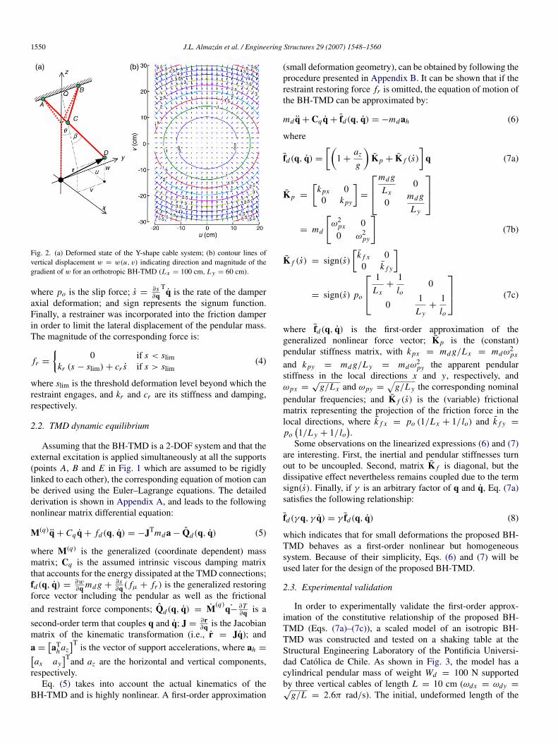
]T. The relationship betweenthe dependent coordinate w and q can be found from Eq. (1).An example of contour lines of w(u, v) can be seen in Fig. 2(b),along with the direction and magnitude of the gradient ofw(u, v), which is related to the restoring force acting on md
due to the gravitational field.The engineering axial deformation s along the direction of
the friction damper is given by:
s(u, v) = ld(u, v) − lo =
√u2 + v2 + (w + lo)2
− lo (2)
where ld(u, v) and lo are the deformed and undeformed lengthsof the device, respectively. The corresponding axial force in thefriction damper is approximated by a rigid-plastic model:
Fig. 2. (a) Deformed state of the Y-shape cable system; (b) contour lines ofvertical displacement w = w(u, v) indicating direction and magnitude of thegradient of w for an orthotropic BH-TMD (Lx = 100 cm, L y = 60 cm).
where po is the slip force; s =∂s∂q
Tq is the rate of the damper
axial deformation; and sign represents the signum function.Finally, a restrainer was incorporated into the friction damperin order to limit the lateral displacement of the pendular mass.The magnitude of the corresponding force is:
fr =
0 if s < slim
kr (s − slim) + cr s if s > slim(4)
where slim is the threshold deformation level beyond which therestraint engages, and kr and cr are its stiffness and damping,respectively.
2.2. TMD dynamic equilibrium
Assuming that the BH-TMD is a 2-DOF system and that theexternal excitation is applied simultaneously at all the supports(points A, B and E in Fig. 1 which are assumed to be rigidlylinked to each other), the corresponding equation of motion canbe derived using the Euler–Lagrange equations. The detailedderivation is shown in Appendix A, and leads to the followingnonlinear matrix differential equation:
M(q)q + Cq q + fd(q, q) = −JTmda − Qd(q, q) (5)
where M(q) is the generalized (coordinate dependent) massmatrix; Cq is the assumed intrinsic viscous damping matrixthat accounts for the energy dissipated at the TMD connections;fd(q, q) =
∂w∂q md g +
∂s∂q ( fµ + fr ) is the generalized restoring
force vector including the pendular as well as the frictional
and restraint force components; Qd(q, q) = M(q)
˙q−∂T∂q is a
second-order term that couples q and q; J =∂r∂q is the Jacobian
matrix of the kinematic transformation (i.e., r = Jq); anda =
[aT
h az]T
is the vector of support accelerations, where ah =[ax ay
]Tand az are the horizontal and vertical components,respectively.
Eq. (5) takes into account the actual kinematics of theBH-TMD and is highly nonlinear. A first-order approximation
(small deformation geometry), can be obtained by following theprocedure presented in Appendix B. It can be shown that if therestraint restoring force fr is omitted, the equation of motion ofthe BH-TMD can be approximated by:
md q + Cq q + fd(q, q) = −mdah (6)
where
fd(q, q) =
[(1 +
az
g
)Kp + K f (s)
]q (7a)
Kp =
[kpx 00 kpy
]=
md g
Lx0
0md g
L y
= md
[ω2
px 00 ω2
py
](7b)
K f (s) = sign(s)
[k f x 00 k f y
]
= sign(s) po
1
Lx+
1lo
0
01
L y+
1lo
(7c)
where fd(q, q) is the first-order approximation of thegeneralized nonlinear force vector; Kp is the (constant)pendular stiffness matrix, with kpx = md g/Lx = mdω2
px
and kpy = md g/L y = mdω2py the apparent pendular
stiffness in the local directions x and y, respectively, andωpx =
√g/Lx and ωpy =
√g/L y the corresponding nominal
pendular frequencies; and K f (s) is the (variable) frictionalmatrix representing the projection of the friction force in thelocal directions, where k f x = po (1/Lx + 1/ lo) and k f y =
po(1/L y + 1/ lo
).
Some observations on the linearized expressions (6) and (7)are interesting. First, the inertial and pendular stiffnesses turnout to be uncoupled. Second, matrix K f is diagonal, but thedissipative effect nevertheless remains coupled due to the termsign(s). Finally, if γ is an arbitrary factor of q and q, Eq. (7a)satisfies the following relationship:
fd(γ q, γ q) = γ fd(q, q) (8)
which indicates that for small deformations the proposed BH-TMD behaves as a first-order nonlinear but homogeneoussystem. Because of their simplicity, Eqs. (6) and (7) will beused later for the design of the proposed BH-TMD.
2.3. Experimental validation
In order to experimentally validate the first-order approx-imation of the constitutive relationship of the proposed BH-TMD (Eqs. (7a)–(7c)), a scaled model of an isotropic BH-TMD was constructed and tested on a shaking table at theStructural Engineering Laboratory of the Pontificia Universi-dad Catolica de Chile. As shown in Fig. 3, the model has acylindrical pendular mass of weight Wd = 100 N supportedby three vertical cables of length L = 10 cm (ωdx = ωdy =√
g/L = 2.6π rad/s). The initial, undeformed length of the
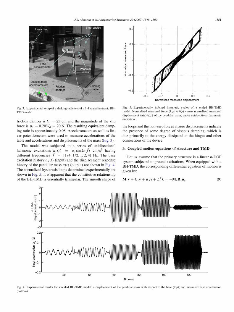
Fig. 3. Experimental setup of a shaking table test of a 1:4 scaled isotropic BH-TMD model.
friction damper is lo = 25 cm and the magnitude of the slipforce is po = 0.20Wd = 20 N. The resulting equivalent damp-ing ratio is approximately 0.08. Accelerometers as well as lin-ear potentiometers were used to measure accelerations of thetable and accelerations and displacements of the mass (Fig. 3).
The model was subjected to a series of unidirectionalharmonic excitations ax (t) = ao sin 2π f t cm/s2 havingdifferent frequencies f = [1/4, 1/2, 1, 2, 4] Hz. The baseexcitation history ax (t) (input) and the displacement responsehistory of the pendular mass u(t) (output) are shown in Fig. 4.The normalized hysteresis loops determined experimentally areshown in Fig. 5; it is apparent that the constitutive relationshipof the BH-TMD is essentially triangular. The smooth shape of
Fig. 5. Experimentally inferred hysteretic cycles of a scaled BH-TMDmodel. Normalized measured force (λx (t)/Wd ) versus normalized measureddisplacement (u(t)/Lx ) of the pendular mass, under unidirectional harmonicexcitation.
the loops and the non-zero forces at zero displacements indicatethe presence of some degree of viscous damping, which isdue primarily to the energy dissipated at the hinges and otherconnections of the device.
3. Coupled motion equations of structure and TMD
Let us assume that the primary structure is a linear n-DOFsystem subjected to ground excitations. When equipped with aBH-TMD, the corresponding differential equation of motion isgiven by:
Ms y + Cs y + Ksy + LTλ = −MsRs ug (9)
Fig. 4. Experimental results for a scaled BH-TMD model: a displacement of the pendular mass with respect to the base (top); and measured base acceleration(bottom).
where yn × 1 is the vector of DOFs of the primary structure;Ms , Ks , and Cs are the mass, stiffness and damping matrices(of order n × n); λ is the interaction force between the pendularmass and the primary structure, L3 × n being a kinematictransformation matrix; ug =
[xg(t) yg(t) zg(t)
]Tis a vectorof ground accelerations; and Rsn × 3 is the input influencevector that relates the components of ug with the structure’sDOFs y.
The interaction force λ can be expressed as:
λ =[λx , λy, λz
]T= md rt
= md (r + a) (10)
where rt= r + a is the total (or absolute) acceleration of the
pendular mass, and
r =ddt
(Jq) = Jq + Jq (11a)
a = Lyt= L
(y + Rs ug
)(11b)
where yt= y + Rs ug is the vector of total accelerations in the
primary structure.Finally, combining Eqs. (9), (10), (11a) and (11b) and Eq.
(5), the final equations of motion of the structure and TMD aregiven by:[
Ms + LTmdL LTmdJJTmdL M(q)
] [yq
]+
[Cs 00 Cq
] [yq
]+
[Ks 00 0
] [yq
]+ · · ·
[0
fd(q, q)
]= −
(Ms + LTmdL)
JTmdL
Rs ug(t) −
[LTmd JqQd(q, q)
](12)
where all second-order terms are on the right-side of theequation. Eq. (12) can be greatly simplified by using the first-order approximation indicated earlier in Eq. (6). Omitting againfr , the equations of motion are given by:[
Ms + LTh mdLh mdLT
h
mdLh M(q)
][yq
]+
[Cs 00 Cq
] [yq
]+ · · ·
Ks 0
0(
1 +az
g
)Kp + K f (s)
[yq
]
= −
[(Ms + LT
h mdLh
)Rs
mdLhRs
]ug(t) (13)
where Lh = L(1 : 2, :) are the first two columns ofL. Please note that Eq. (13) does not include second-orderterms. Furthermore, the only nonlinear term is the functionsign(s) contained in K f (s), which considerably reducesthe computational effort necessary to perform numericalintegrations. It will be shown later, however, that strong groundmotions induce large deformations in the BH-TMD and, hence,the exact equations of motion should be used in such cases toobtain an accurate solution.
4. Design of the proposed BH-TMD
It is well-known that the efficiency of a TMD is sensitiveprimarily to the tuning of the fundamental frequency ωd , and toa lesser extent of the damping ratio ξd . Optimal values of theseparameters for an undamped linear SDOF system subjected toa white-noise excitation are given by [10]:
Ωop =ωd
ωs=
√1 − µ/21 + µ
(14)
ξop =
√µ (1 − µ/4)
4 (1 + µ) (1 − µ/2)(15)
where µ is the ratio between the mass of the TMD and thatof the primary structure; and ωd and ωs are the fundamentalnominal frequencies of the TMD and that of the structure in thedirection considered, respectively. Based on these equations (oron any of the equivalent equations proposed in the literature[11–13]), valid for linear behavior, simple design equations forthe BH-TMD can be easily derived. Because of its orthotropicproperties, the BH-TMD can be tuned in each principaldirection independently, and the pendular lengths are given by(Eq. (7b)):
Lx =g
ω2px
=g
Ω2opω
2sx
(16)
L y =g
ω2py
=g
Ω2opω
2sy
. (17)
An expression for the optimal value of the slip force pocan be obtained by considering the equivalent viscous dampingratio ξeq . Assuming harmonic motion of amplitude uo in thex-direction, the total equivalent viscous damping is given by:
ξeq = ξo + ξ f = ξo +1
4π
Ed
Es(18)
where Ed = 2k f x u2o is the energy dissipated by friction in one
cycle; Es =12 kpx u2
o is the maximum potential energy storedin the system; ξ f =
14π
EdEs
is the so called frictional dampingratio; and ξo is the intrinsic viscous damping ratio that takesinto account the energy dissipated in the connections.
Setting ξeq = ξop, and substituting kpx and k f x by thecorresponding expressions indicated in Eqs. (7b) and (7c), itcan be shown that:
po =po
md g=
(ξop − ξo
)π
(1 + Lx/ lo)(19)
where po is the optimal slip force, normalized by the weightof the pendular mass. Notice that the optimal value for they-direction is obtained by substituting Lx by L y in Eq. (19),which gives a greater value of po (remember that Lx > L y). Apossible solution for this inconsistency is to adopt a value of pofor the direction in which a higher degree of control is required.In a true building, however, this inconsistency is essentiallyirrelevant, since the performance of TMDs is rather insensitiveto the damping ratio in the neighborhood of the optimal value.
Fig. 6. Thin-walled cylindrical steel chimney considered in this study (modelM1).
Based on this observation, the smallest of the values of po givenby Eq. (19) is adopted in this study.
5. Structures, response quantities, and ground motions
Two nominally symmetric structural models are consideredin this study. The first one, denoted as model M1 (Fig. 6) isa steel chimney typically found in copper processing plants.The height of the structure is 80 m, the diameter is 3 m,and the average mantle thickness is 0.02 m. The fundamentalfrequencies are ωx = ωy = 1.37π rad/s, where perpendiculardirections X and Y may have any orientation. It is assumed thatan isotropic TMD is incorporated at the top of the structure,as shown in Fig. 6. Torsional effects due to the eccentriclocation of the TMD will not be taken into account. The secondmodel, denoted M2 (Fig. 7) is a 25-story reinforced concretebuilding designed to the current Chilean seismic code. Thecorresponding fundamental frequencies are ωx = 1.05π andωy = 1.4ωx in the X and Y directions, respectively. It isassumed that an orthotropic TMD has been attached to the rooflevel at the center of mass of the structure.
For comparison, two types of TMDs are included in eachof the structural models: (i) the proposed BH-TMD; and(ii) an “ideal” bidirectional linear TMD with viscous energydissipation. The latter, denoted BLV-TMD, is shown in Fig. 8.The practical implementation of the BLV-TMD requires thatboth the springs and the viscous dampers behave linearlyeven when subjected to large deformations. The dynamicproperties of the structural models and corresponding TMDsare summarized in Table 1. The properties of the TMDs wereselected using design equation (14)–(19).
The efficiency of the TMDs in reducing an arbitrary responsequantity r(t) is evaluated through the following reductionfactors:
Ψ1 = 1 −(r + σr )controlled
(r + σr )uncontrolled(20)
(a) Plan view of a typical building story.
(b) Resisting planes 1, 2, and 3.
Fig. 7. 25-story R/C building considered in this study (model M2).
Fig. 8. Schematic plan view of the Bidirectional Linear Viscous Tuned MassDamper (BLV-TMD) used as benchmark device.
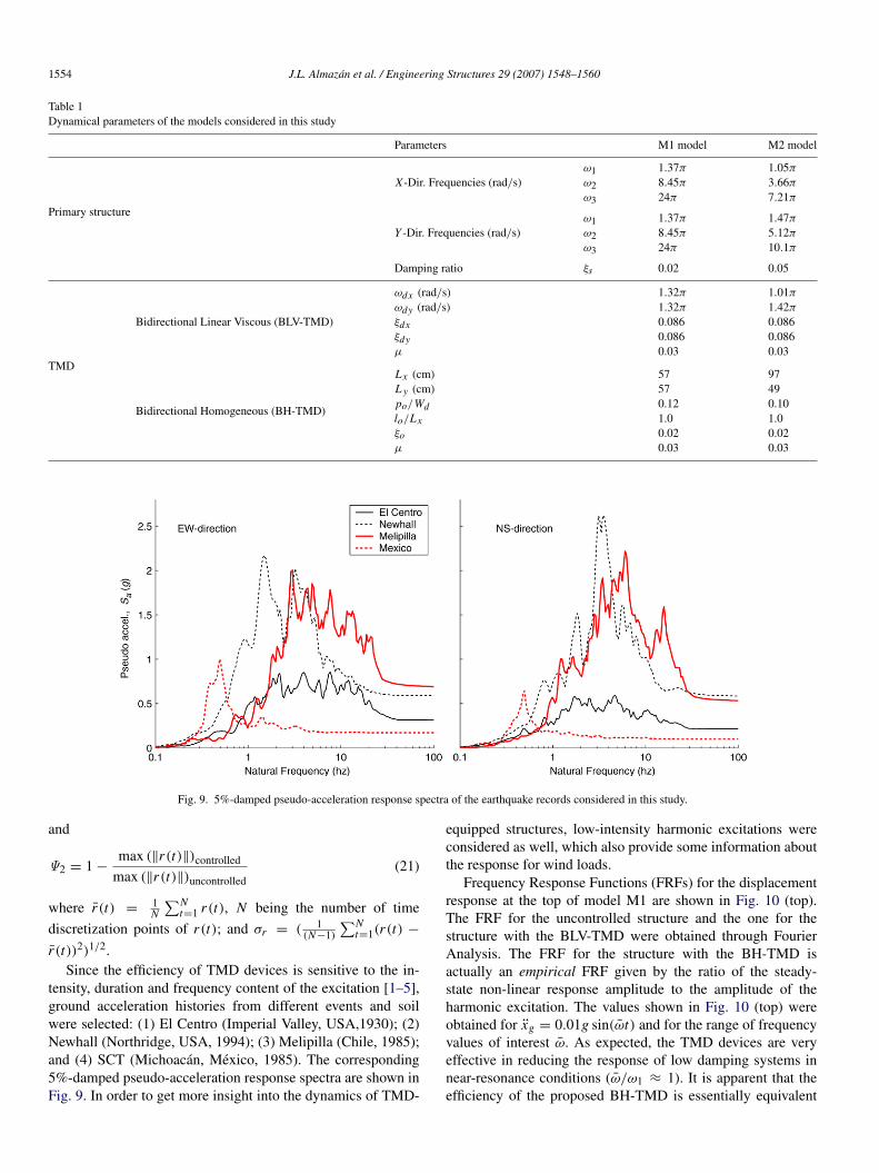
Fig. 9. 5%-damped pseudo-acceleration response spectra of the earthquake records considered in this study.
and
Ψ2 = 1 −max (‖r(t)‖)controlled
max (‖r(t)‖)uncontrolled(21)
where r(t) =1N
∑Nt=1 r(t), N being the number of time
discretization points of r(t); and σr = ( 1(N−1)
∑Nt=1(r(t) −
r(t))2)1/2.Since the efficiency of TMD devices is sensitive to the in-
tensity, duration and frequency content of the excitation [1–5],ground acceleration histories from different events and soilwere selected: (1) El Centro (Imperial Valley, USA,1930); (2)Newhall (Northridge, USA, 1994); (3) Melipilla (Chile, 1985);and (4) SCT (Michoacan, Mexico, 1985). The corresponding5%-damped pseudo-acceleration response spectra are shown inFig. 9. In order to get more insight into the dynamics of TMD-
equipped structures, low-intensity harmonic excitations wereconsidered as well, which also provide some information aboutthe response for wind loads.
Frequency Response Functions (FRFs) for the displacementresponse at the top of model M1 are shown in Fig. 10 (top).The FRF for the uncontrolled structure and the one for thestructure with the BLV-TMD were obtained through FourierAnalysis. The FRF for the structure with the BH-TMD isactually an empirical FRF given by the ratio of the steady-state non-linear response amplitude to the amplitude of theharmonic excitation. The values shown in Fig. 10 (top) wereobtained for xg = 0.01g sin(ωt) and for the range of frequencyvalues of interest ω. As expected, the TMD devices are veryeffective in reducing the response of low damping systems innear-resonance conditions (ω/ω1 ≈ 1). It is apparent that theefficiency of the proposed BH-TMD is essentially equivalent
Fig. 10. Response to harmonic excitations (PGA = 0.01g) of model M1, with and without TMDs: (a) Frequency Response Functions (FRFs) for the displacementat the top of the chimney; (b) response histories under resonance condition of normalized interaction force (left) and normalized displacement at the top of thechimney (right).
to that of the BLV-TMD, which is slightly more efficient forω < ω1, and slightly less efficient for ω > ω1. Responsetime histories, obtained by considering resonance conditions,can be seen at the bottom of Fig. 10. The left plot showsthe history of the normalized interaction force λx = λx/Wd ,while the right plot shows the history of the displacementresponse at the top of the chimney, normalized by the peakuncontrolled response. It can be seen that the displacementresponse histories of the structure with the TMD devices is only7% of that for the uncontrolled case, and that both responsesare essentially identical to each other. Please note that thedisplacement response history for the structure with the BH-TMD is essentially a perfect harmonic function, even thoughthe interaction force λx is clearly nonlinear.
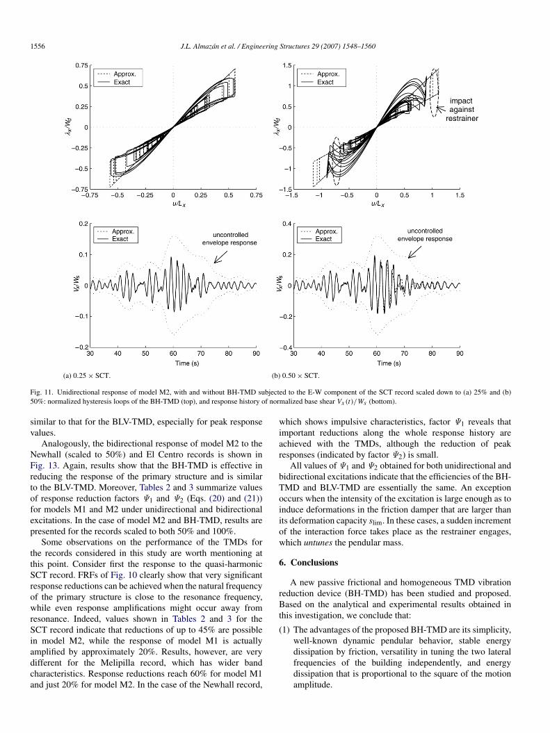
A comparison between results obtained using the exactformulation for the BH-TMD (Eq. (12)) and results obtainedusing the approximate formulation (Eq. (13)) is shown inFig. 11. These results were obtained considering the M2model subjected to the E-W component of the SCT recordscaled to: (a) 25% (left plots); and (b) 50% (right plots). Thenormalized hysteresis loops (λx/Wd vs. u/Lx ) show that theactual constitutive relationship of the BH-TMD is essentiallytriangular for displacements less than 0.3Lx , and that changesin stiffness are noticeable only for larger displacements. Suchchanges occur as a result of two actions in the tensile forces inthe cables: (i) an initial increase due to centripetal accelerations
an = u2/Lx (velocity hardening); and (ii) a decrease at largedeformations due to a lesser influence of the weight of thependular mass Wd (deformation softening). The response of theprimary structure, however, does not seem to be affected bythese effects, as shown by the corresponding normalized baseshear response history Vx (t)/Ws (bottom plot of Fig. 11(a)).On the other hand, the right-side normalized hysteresis loopsindicate that the deformation capacity of the friction damperis reached in this case (s = slim), which creates a suddenincrease in stiffness due to engagement of the restrainer.Some differences between the exact and approximate responses(bottom plot of Fig. 11(b)) are now observed in the 60–80 stime window. However, the response of the structure withthe BH-TMD is still very satisfactory because model M2 isnearly in resonance with the quasi-harmonic seismic excitationconsidered in this case.
Shown in Fig. 12 is the bidirectional response of model M1,with and without TMDs, to the Melipilla and El Centro records.The left-side plots show displacement paths at the top of thechimney, dx (t) vs. dy(t); while the right-side plots show the
response history of total displacement d(t) =
√d2
x (t) + d2y (t).
The uncontrolled response shows greater displacements inthe direction for which ground accelerations are larger; thesedisplacements are the ones most effectively reduced by theTMDs, leading to a balance in the plus and minus direction.Please observe that the response for the BH-TMD is very
Fig. 11. Unidirectional response of model M2, with and without BH-TMD subjected to the E-W component of the SCT record scaled down to (a) 25% and (b)50%: normalized hysteresis loops of the BH-TMD (top), and response history of normalized base shear Vx (t)/Ws (bottom).
similar to that for the BLV-TMD, especially for peak responsevalues.
Analogously, the bidirectional response of model M2 to theNewhall (scaled to 50%) and El Centro records is shown inFig. 13. Again, results show that the BH-TMD is effective inreducing the response of the primary structure and is similarto the BLV-TMD. Moreover, Tables 2 and 3 summarize valuesof response reduction factors Ψ1 and Ψ2 (Eqs. (20) and (21))for models M1 and M2 under unidirectional and bidirectionalexcitations. In the case of model M2 and BH-TMD, results arepresented for the records scaled to both 50% and 100%.
Some observations on the performance of the TMDs forthe records considered in this study are worth mentioning atthis point. Consider first the response to the quasi-harmonicSCT record. FRFs of Fig. 10 clearly show that very significantresponse reductions can be achieved when the natural frequencyof the primary structure is close to the resonance frequency,while even response amplifications might occur away fromresonance. Indeed, values shown in Tables 2 and 3 for theSCT record indicate that reductions of up to 45% are possiblein model M2, while the response of model M1 is actuallyamplified by approximately 20%. Results, however, are verydifferent for the Melipilla record, which has wider bandcharacteristics. Response reductions reach 60% for model M1and just 20% for model M2. In the case of the Newhall record,
which shows impulsive characteristics, factor Ψ1 reveals thatimportant reductions along the whole response history areachieved with the TMDs, although the reduction of peakresponses (indicated by factor Ψ2) is small.
All values of Ψ1 and Ψ2 obtained for both unidirectional andbidirectional excitations indicate that the efficiencies of the BH-TMD and BLV-TMD are essentially the same. An exceptionoccurs when the intensity of the excitation is large enough as toinduce deformations in the friction damper that are larger thanits deformation capacity slim. In these cases, a sudden incrementof the interaction force takes place as the restrainer engages,which untunes the pendular mass.
6. Conclusions
A new passive frictional and homogeneous TMD vibrationreduction device (BH-TMD) has been studied and proposed.Based on the analytical and experimental results obtained inthis investigation, we conclude that:
(1) The advantages of the proposed BH-TMD are its simplicity,well-known dynamic pendular behavior, stable energydissipation by friction, versatility in tuning the two lateralfrequencies of the building independently, and energydissipation that is proportional to the square of the motionamplitude.
Fig. 12. Bidirectional response of chimney (model M1) with and without TMDs, to two earthquake records: (a) Melipilla; and (b) El Centro. Displacement pathsare shown at left and response history of total displacement d(t) at the top of the chimney at right.
Table 2Maximum uncontrolled response (in % of total height H ), and reduction factors Ψ1 and Ψ2 (in brackets) for chimney (model M1)
(2) The evaluation of the response of two different structuralmodels subjected to different unidirectional and bidirec-tional ground excitations shows that the level of responsereduction that can be achieved by the BH-TMD is similarto that of an ideal linear viscous TMD; the BH-TMD be-came less effective only when the deformation capacity ofthe friction damper is reached and the restraint engages dueto excessive displacement of the pendular mass.
(3) Depending on the excitation and structure, the BH-TMDmay reach displacement reduction factors that vary from a
few percentage points to 60%.(4) Experimental results obtained through shaking table tests
of a scaled model of an isotropic BH-TMD demonstratethat the proposed device is a realization of an homogeneousdevice, i.e., its fundamental period and equivalent dampingratio are essentially independent of the vibration amplitude.
Acknowledgements
This investigation has been supported by the PontificiaUniversidad Catolica de Chile under Grant DIPEI 2002/09E,
Fig. 13. Bidirectional response of 25-story building (model M2) with and without TMDs, to two earthquake records: (a) Newhall scaled to 50%; and (b) El Centro.Displacement paths are shown at left and response history of total roof displacement d(t) at right.
Table 3Maximum uncontrolled response (in % of total height H ), and reduction factors Ψ1 and Ψ2 (in brackets) for 25-story building (model M2)
(dissipative forces), Cq = ξoI the assumed intrinsic viscousdamping matrix of the device that takes into account the energydissipated in the connections (I is a 2 × 2 identity matrix in thiscase); and Qe = JTmda is the generalized external force (inputforce), a the vector of total accelerations at the supports and
J =∂r∂q =
[∂r∂u
∂r∂v
]is the Jacobian matrix.
Equivalent expressions for the five terms of Eq. (A.1) can beobtained as shown below:(1) First term, d
dt∂T∂q
ddt
∂T
∂q=
ddt
(M(q)q
)= M(q)q + M
(q)q (A.2)
where M(q)= JTM(r)J is the generalized mass matrix.
(2) Second term, ∂T∂q
∂T
∂q j=
∂ r∂q j
T ∂T
∂ r=
(∂J∂q j
q)T
M(r)r
= qT
(∂J∂q j
T
M(r)J
)q = qTH j q. (A.3)
(3) Third term, ∂Vg∂q
∂Vg
∂q=
∂w
∂qmd g. (A.4)
(4) Fourth term, Qi
Qi =∂s
∂q
(fµ + fr
)+ Cq q =
∂rT
∂q∂s
∂r
(fµ + fr
)+ Cq q = JT ∂s
∂r
(fµ + fr
)+ Cq q (A.5)
where ∂s∂r can be obtained using Eq. (2).
(5) Fifth term, Qe
Qe = JTmda =
[I
∂w
∂q
]md
[ahaz
]= mdah + md
∂w
∂qaz . (A.6)
Substituting Eqs. (A.2)–(A.6) into Eq. (A.1) gives Eq. (5).
Appendix B. First-order approximation of Eq. (5)
This appendix shows the derivation of the first-orderapproximation of Eq. (5), which has four nonlinear terms: (i)ddt
∂T∂q ; (ii) ∂T
∂q ; (iii) ∂w∂q ; y (iv) ∂s
∂q .
(i) Term ddt
∂T∂q = M(q)q + M
(q)q (Eq. (A.2))
ddt
∂T
∂ qi=
∑j
m(q)i j q j + m(q)
i j q j (B.1)
where m(q)i j = M(q)(i, j) can be expressed by a Taylor series
as:
m(q)i j = m(q)
i j |0 +
∑k
∂m(q)i j
∂qk
∣∣∣∣∣∣0
qk + ϑ2(q) (B.2)
where ()|0 denotes the function () evaluated at q = 0; and ϑ2(q)
represents the nonlinear terms. In addition, m(q)i j =
ddt (m
(q)i j )
can be written as:
m(q)i j =
∑k
∂m(q)i j
∂qkqk . (B.3)
Substitution of (B.2) and (B.3) into (B.1) gives:
ddt
∂T
∂qi=
∑j
m(q)i j
∣∣∣0q j +
∑j
∑k
∂m(q)i j
∂qk
∣∣∣∣∣∣0
qk + ϑ2(q)
q j
+
∑j
∑k
∂m(q)i j
∂qkq j qk . (B.4)
Clearly, only the first term of (B.4) is linear, i.e.:
ddt
∂T
∂qi≈
∑j
m(q)i j
∣∣∣0q j (B.5)
or
ddt
∂T
∂q≈ M
(q)q; M (q)
= md
[1 00 1
](B.6)
where M(q)
is the local mass matrix evaluated at q = 0.(ii) Term ∂T
∂q
T = 1/2∑
i
∑j
m(q)i j qi q j (B.7)
∂T
∂qk=
∑i
∑j
∂m(q)i j
∂qkqi q j . (B.8)
Obviously, expression (B.8) does not include linear terms,i.e.:
∂T
∂q≈ 0. (B.9)
(iii) Term ∂w∂q
The i th component of vector ∂w∂q can be expressed by a
Taylor series as:
∂w
∂qi=
∂w
∂qi
∣∣∣∣0+
∑j
∂2w
∂qi∂q j
∣∣∣∣0q j + ϑ2(q) (B.10)
where ∂w∂qi
∣∣∣0
= 0. Hence, the linear approximation of ∂w∂q can be
∂qIn this case, the procedure followed to linearize terms (i) and
(iii) leads to:
∂s
∂q≈ Hsq; Hs =
1
Lx+
1lo
0
01
L y+
1lo
(B.12)
where Hs(i, j) =∂2s
∂qi ∂q j
∣∣∣0
is the Hessian matrix of s(q)
evaluated at q = 0.Substituting Eqs. (B.6), (B.9), (B.11) and (B.12) into Eq. (5)
gives Eq. (6).
References
[1] Villaverde R, Koyama LA. Damped resonants appendages to increaseinherent damping in buildings. Earthq Eng Struct Dyn 1993;22:491–508.
[2] Bernal J. Influence of ground motion characteristic on the effectiveness oftuned mass dampers. In: Proc. XI world conf. on earthq. engng. 1996.
[3] Ruiz SE, Esteva L. About the effectiveness of tuned mass damperson nonlinear systems subjected to earthquakes. In: Manolis GD,Beskos DE, Brebbia CA, editors. Earthquake resistant engineering
[4] Soto-Brito R, Ruiz SE. Influence of ground motion intensity on theeffectiveness of tuned mass dampers. Earthq Eng Struct Dyn 1999;28:1255–71.
[5] Lukkunaprasit P, Wanitkorkul A. Inelastic buildings with tuned massdampers under moderate ground motions from distant earthquakes. EarthqEng Struct Dyn 2001;30:537–51.
[6] Pinkaew T, Lukkunaprasit P, Chucapote P. Seismic effectiveness of tunedmass dampers for damage reduction of structures. Eng Struct 2003;25:39–46.
[7] Lin C, Ueng J, Huang T. Seismic response reductions of irregularbuildings using passive tuned mass dampers. Eng Struct 1999;22:513–24.
[8] Singh M, Singh S, Moreschi L. Tuned mass dampers for response controlof torsional buildings. Earthq Eng Struct Dyn 2002;31:749–69.
[9] Inaudi J, Kelly J. Mass damper using friction-dissipating devices. J EngMech 1995;121:142–9.
[10] Warburton G. Optimum absorber parameters for various combinationsof response and excitation parameters. Earthq Eng Struct Dyn 1982;10:381–401.
[11] Villaverde R. Reduction in seismic response with heavily dampedvibration absorbers. Earthq Eng Struct Dyn 1985;13:33–42.
[12] Fujino Y, Abe M. Design formulas for tuned mass dampers based on aperturbation technique. Earthq Eng Struct Dyn 1993;22:833–54.
[13] Sadek F, Mohraz B, Taylor A, Chung R. A method of estimating theparameters of tuned mass dampers for seismic applications. Earthq EngStruct Dyn 1997;26:617–35.


![Adaptive passive, semiactive, smart tuned mass dampers ... · The smart tuned mass damper (STMD) and smart multiple tuned mass damper, developed by the author and his coworkers [31,32,36],](https://static.documents.pub/doc/80x56/5ebe7ddef1f48b66695f2c9f/adaptive-passive-semiactive-smart-tuned-mass-dampers-the-smart-tuned-mass.jpg)


Reduction of Wind Induced Motion Utilizing a Tuned Sloshing Damper](https://static.documents.pub/doc/80x56/577d21d61a28ab4e1e960032/21990reduction-of-wind-induced-motion-utilizing-a-tuned-sloshing-damper.jpg)

