A Brief

Introduction To

The SISO Design

Tool Lecture notes for the seminars ‘An Introduction

to Matlab & Examples from Control Theory’ Aristotle University of Thessaloniki, Faculty of Sciences, Department of Mathematics

2012

Moysis Lazaros

A Brief Introduction To the SISO Design Tool – Moysis Lazaros

For any questions, corrections or comments feel free to contact me:

Moysis Lazaros

M.Sc. student ‘Theoretical Informatics & Control Systems and Theory’.

Department of Mathematics, AUTH.

E-mail: moysis.lazaros@hotmail.com

A Brief Introduction To the SISO Design Tool – Moysis Lazaros

3

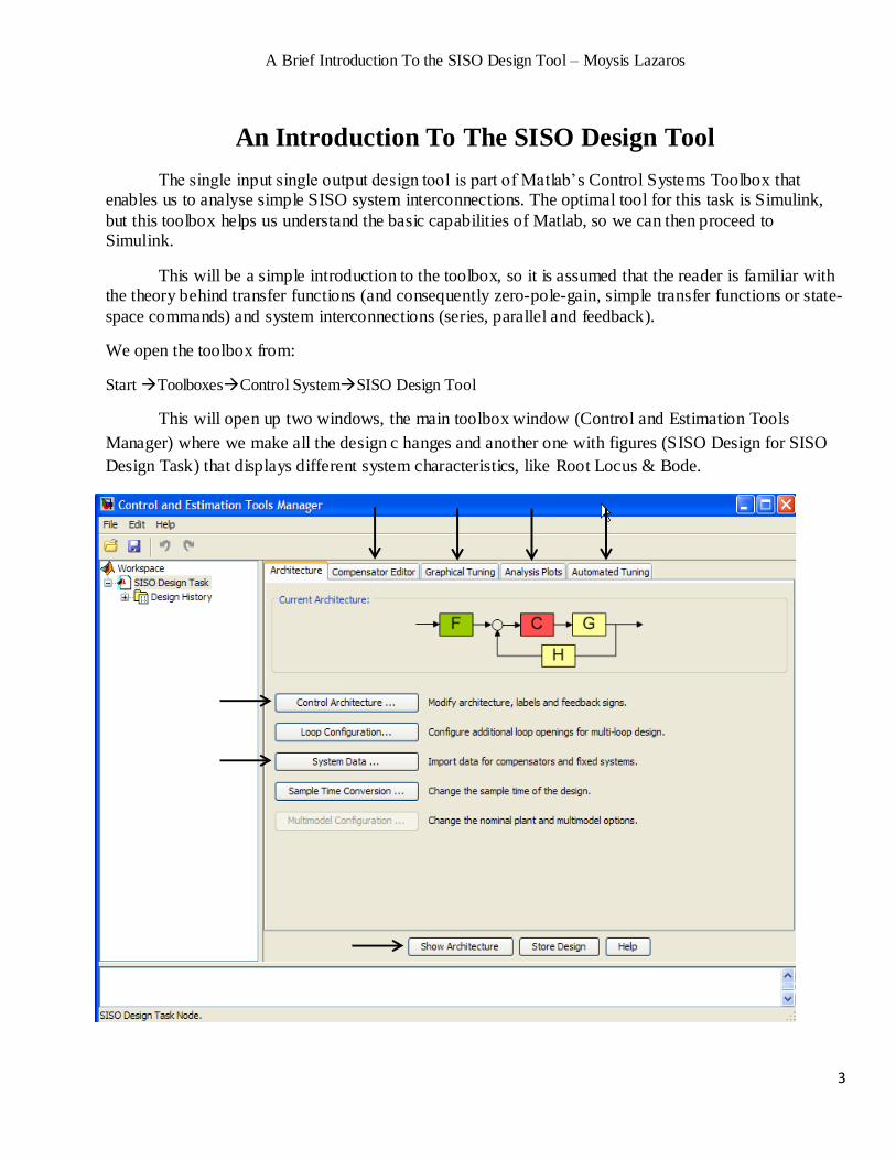
An Introduction To The SISO Design Tool

The single input single output design tool is part of Matlab’s Control Systems Toolbox that enables us to analyse simple SISO system interconnections. The optimal tool for this task is Simulink,

but this toolbox helps us understand the basic capabilities of Matlab, so we can then proceed to Simulink.

This will be a simple introduction to the toolbox, so it is assumed that the reader is familiar with the theory behind transfer functions (and consequently zero-pole-gain, simple transfer functions or state-

space commands) and system interconnections (series, parallel and feedback).

We open the toolbox from:

Start ToolboxesControl SystemSISO Design Tool

This will open up two windows, the main toolbox window (Control and Estimation Tools

Manager) where we make all the design c hanges and another one with figures (SISO Design for SISO

Design Task) that displays different system characteristics, like Root Locus & Bode.

A Brief Introduction To the SISO Design Tool – Moysis Lazaros

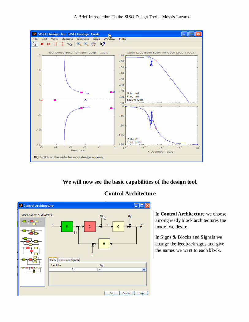
We will now see the basic capabilities of the design tool.

Control Architecture

In Control Architecture we choose

among ready block architectures the

model we desire.

In Signs & Blocks and Signals we

change the feedback signs and give

the names we want to each block.

A Brief Introduction To the SISO Design Tool – Moysis Lazaros

5

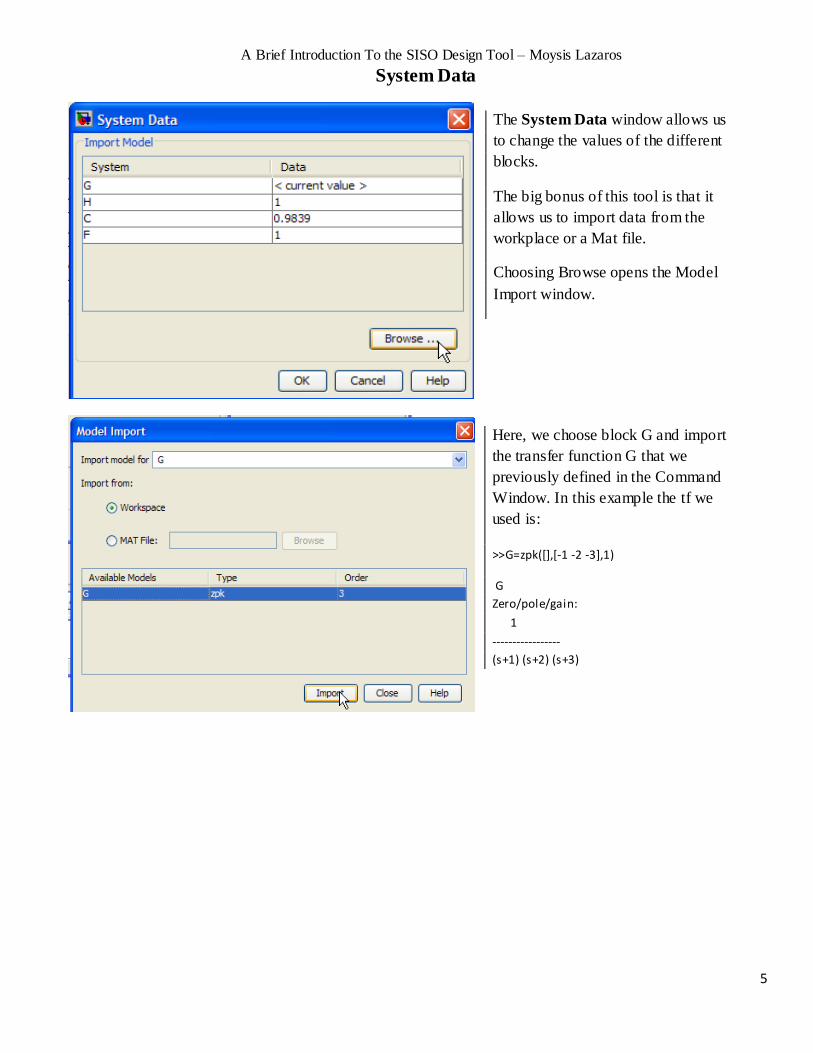
System Data

The System Data window allows us

to change the values of the different

blocks.

The big bonus of this tool is that it

allows us to import data from the

workplace or a Mat file.

Choosing Browse opens the Model

Import window.

Here, we choose block G and import

the transfer function G that we

previously defined in the Command

Window. In this example the tf we

used is:

>>G=zpk([],[-1 -2 -3],1)

G

Zero/pole/gain:

1

-----------------

(s+1) (s+2) (s+3)

A Brief Introduction To the SISO Design Tool – Moysis Lazaros

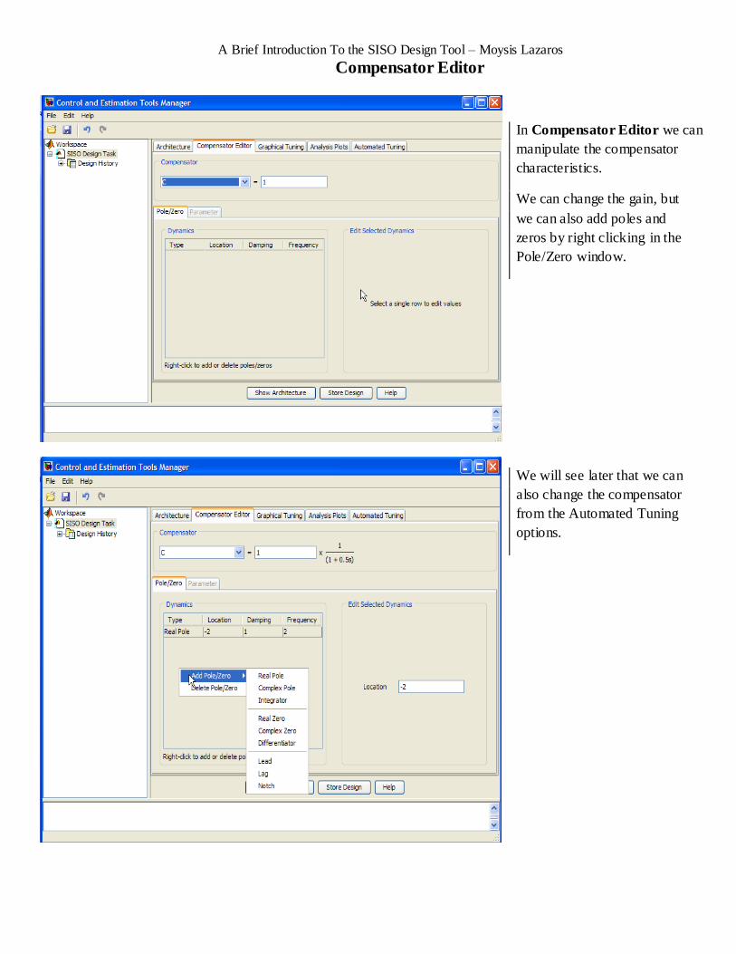
Compensator Editor

In Compensator Editor we can

manipulate the compensator

characteristics.

We can change the gain, but

we can also add poles and

zeros by right clicking in the

Pole/Zero window.

We will see later that we can

also change the compensator

from the Automated Tuning

options.

A Brief Introduction To the SISO Design Tool – Moysis Lazaros

7

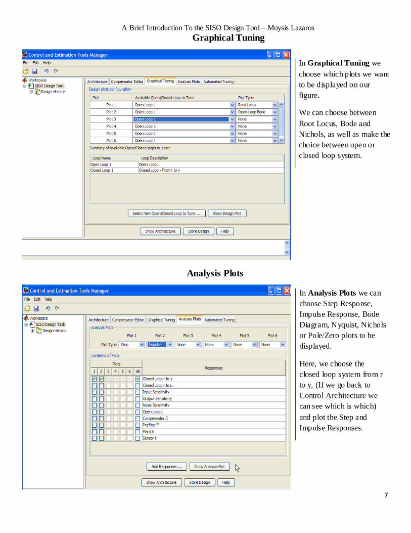
Graphical Tuning

Analysis Plots

In Graphical Tuning we

choose which plots we want

to be displayed on our

figure.

We can choose between

Root Locus, Bode and

Nichols, as well as make the

choice between open or

closed loop system.

In Analysis Plots we can

choose Step Response,

Impulse Response, Bode

Diagram, Nyquist, Nichols

or Pole/Zero plots to be

displayed.

Here, we choose the

closed loop system from r

to y, (If we go back to

Control Architecture we

can see which is which)

and plot the Step and

Impulse Responses.

A Brief Introduction To the SISO Design Tool – Moysis Lazaros

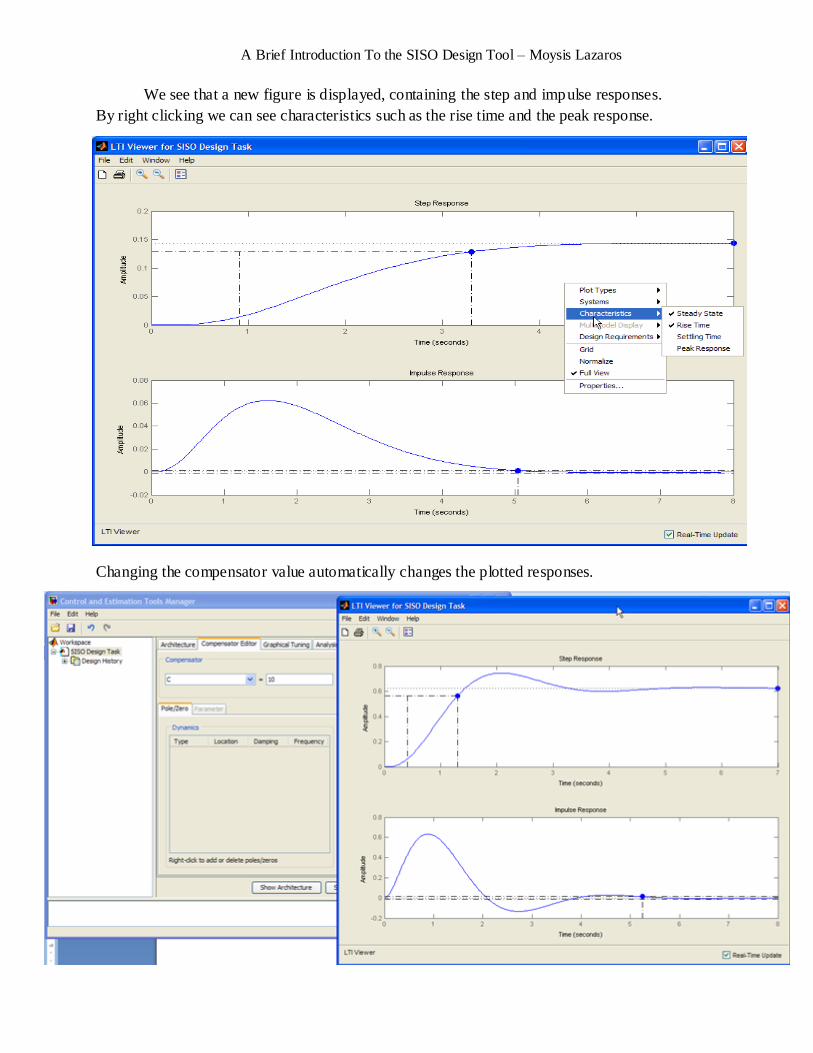
We see that a new figure is displayed, containing the step and impulse responses.

By right clicking we can see characteristics such as the rise time and the peak response.

Changing the compensator value automatically changes the plotted responses.

A Brief Introduction To the SISO Design Tool – Moysis Lazaros

9

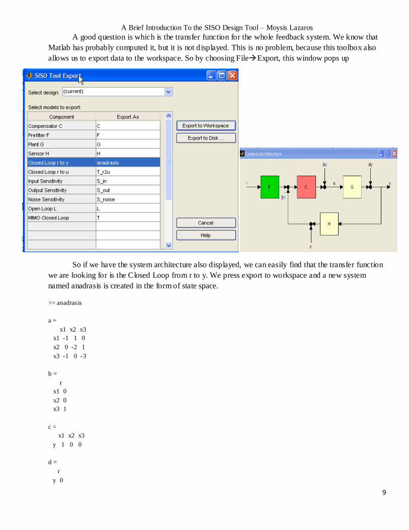
A good question is which is the transfer function for the whole feedback system. We know that

Matlab has probably computed it, but it is not displayed. This is no problem, because this toolbox also

allows us to export data to the workspace. So by choosing FileExport, this window pops up

So if we have the system architecture also displayed, we can easily find that the transfer function

we are looking for is the Closed Loop from r to y. We press export to workspace and a new system

named anadrasis is created in the form of state space.

>> anadrasis

a =

x1 x2 x3

x1 -1 1 0

x2 0 -2 1

x3 -1 0 -3

b =

r

x1 0

x2 0

x3 1

c =

x1 x2 x3

y 1 0 0

d =

r

y 0

A Brief Introduction To the SISO Design Tool – Moysis Lazaros

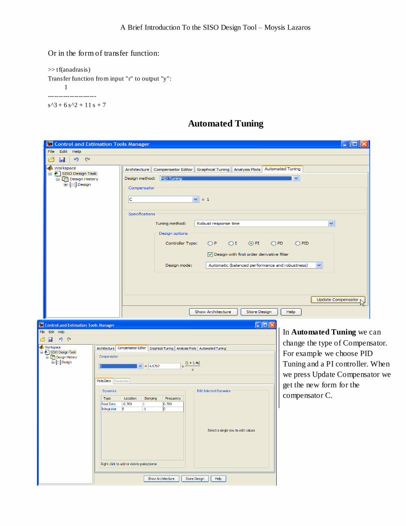
Or in the form of transfer function:

>> t f(anadrasis)

Transfer function from input "r" to output "y":

1

----------------------

s^3 + 6 s^2 + 11 s + 7

Automated Tuning

In Automated Tuning we can

change the type of Compensator.

For example we choose PID

Tuning and a PI controller. When

we press Update Compensator we

get the new form for the

compensator C.

A Brief Introduction To the SISO Design Tool – Moysis Lazaros

11

This concludes our basic analysis of the Control Systems Toolbox. There are some features we

did not dive into, yet we covered all the basic parts and features one needs to know. The next big step

from here is to get to know Simulink, an environment capable of designing all kinds of systems and real-

time applications.

As an exercise, you can study the case of C=-6. Check out the step and impulse responses. Do

you find the result unexpected? In order to understand this result, take a look at the closed loop transfer

function and it’s solution. Is this system stable? Is it BIBO (bounded- input bounded-output) stable?

A Brief Introduction To the SISO Design Tool – Moysis Lazaros

References 1. Mathworks Control System Toolbox videos & examples

http://www.mathworks.com/products/control/examples.html.

2. N. Karampetakis. Lecture notes for MSc course Computer Aided Control Systems, Dept. of

Mathematics AUTH.

3. A.I. Vardulakis, Εισαγωγή στη Μαθηματική Θεωρία Σημάτων, Συστημάτων και Ελέγχου Τόμος

Α΄. Εκδόσεις Τζιόλα 2012.