A CASE STUDY OF BAN DAN NA KHAM WATERSHED, THAILAND

SENSITIVITY ANALYSIS OF SOILGRIDS250M DATA FOR SOIL EROSION MODELLING: A CASE STUDY OF BAN DAN NA KHAM WATERSHED, THAILAND

CHIKE ONYEKA MADUEKE

FEBRUARY 2019

SUPERVISORS:

Dr. D.P.K. Shrestha Dr. P. Nyktas

SENSITIVITY ANALYSIS OF SOILGRIDS250M DATA FOR SOIL EROSION MODELLING: A CASE STUDY OF BAN DAN NA KHAM WATERSHED, THAILAND

CHIKE ONYEKA MADUEKE

Enschede, The Netherlands

February 2019

Thesis submitted to the Faculty of Geo-Information Science

and Earth Observation of the University of Twente in partial

fulfilment of the requirements for the degree of Master of

Science in Geo-information Science and Earth Observation.

Specialization: Natural Resources Management

SUPERVISORS:

Dr. D.P.K. Shrestha Dr. P. Nyktas

THESIS ASSESSMENT BOARD:

Prof. Dr. Victor G. Jetten (Chair)

Dr. Jeroen Schoorl (External Examiner, Wageningen

University & Research Centre)

DISCLAIMER

This document describes work undertaken as part of a programme of study at the Faculty of Geo-Information Science

and Earth Observation of the University of Twente. All views and opinions expressed therein remain the sole

responsibility of the author, and do not necessarily represent those of the Faculty.

Sensitivity Analysis of SoilGrids250m Data for Soil Erosion Modelling: A Case Study of Ban Dan Na Kham Watershed, Thailand

i

ABSTRACT

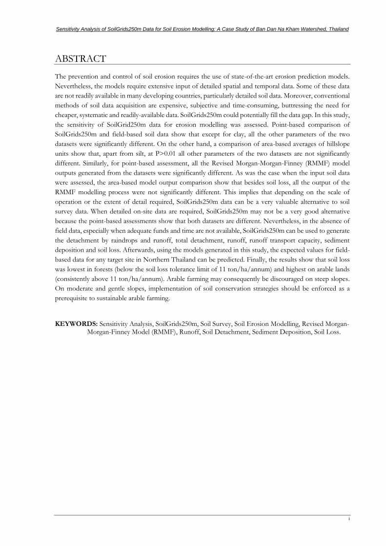
The prevention and control of soil erosion requires the use of state-of-the-art erosion prediction models.

Nevertheless, the models require extensive input of detailed spatial and temporal data. Some of these data

are not readily available in many developing countries, particularly detailed soil data. Moreover, conventional

methods of soil data acquisition are expensive, subjective and time-consuming, buttressing the need for

cheaper, systematic and readily-available data. SoilGrids250m could potentially fill the data gap. In this study,

the sensitivity of SoilGrid250m data for erosion modelling was assessed. Point-based comparison of

SoilGrids250m and field-based soil data show that except for clay, all the other parameters of the two

datasets were significantly different. On the other hand, a comparison of area-based averages of hillslope

units show that, apart from silt, at P>0.01 all other parameters of the two datasets are not significantly

different. Similarly, for point-based assessment, all the Revised Morgan-Morgan-Finney (RMMF) model

outputs generated from the datasets were significantly different. As was the case when the input soil data

were assessed, the area-based model output comparison show that besides soil loss, all the output of the

RMMF modelling process were not significantly different. This implies that depending on the scale of

operation or the extent of detail required, SoilGrids250m data can be a very valuable alternative to soil

survey data. When detailed on-site data are required, SoilGrids250m may not be a very good alternative

because the point-based assessments show that both datasets are different. Nevertheless, in the absence of

field data, especially when adequate funds and time are not available, SoilGrids250m can be used to generate

the detachment by raindrops and runoff, total detachment, runoff, runoff transport capacity, sediment

deposition and soil loss. Afterwards, using the models generated in this study, the expected values for field-

based data for any target site in Northern Thailand can be predicted. Finally, the results show that soil loss

was lowest in forests (below the soil loss tolerance limit of 11 ton/ha/annum) and highest on arable lands

(consistently above 11 ton/ha/annum). Arable farming may consequently be discouraged on steep slopes.

On moderate and gentle slopes, implementation of soil conservation strategies should be enforced as a

prerequisite to sustainable arable farming.

KEYWORDS: Sensitivity Analysis, SoilGrids250m, Soil Survey, Soil Erosion Modelling, Revised Morgan-Morgan-Finney Model (RMMF), Runoff, Soil Detachment, Sediment Deposition, Soil Loss.

ii

ACKNOWLEDGEMENTS

I want to use this opportunity to express my profound gratitude to the government and people of

Netherlands, to NUFFIC and to the Faculty of Geoinformation Science and Earth Observation, University

of Twente, Enschede, for granting me the NFP fellowship that made it possible for me to be here today.

Furthermore, my heartfelt gratitude goes to the management and staff of Nnamdi Azikiwe University

(UNIZIK), Awka, Nigeria for granting the study leave that enabled me to pursue my dreams. Also worthy

of special mention, are the Head, Department of Soil Science and Land Resources Management, UNIZIK,

Awka, Prof. Peter C. Nnabude, Prof. Frank O.R. Akamigbo, Prof. Charles L.A. Asadu and Dr. Akudo

Onunwa. Thank you for your magnanimity and support over the years.

To my supervisors, Dr. D.P.K. Shrestha and Dr. P. Nyktas, I owe a debt of gratitude. Thank you very much

for your patience, advice, tutelage, guidance and psychological support, even in the heart of the storm. Dr.

D.P.K. Shrestha, I must thank you once more for an enlightening trip to Thailand, fraught with numerous

ups and downs. Also worthy of note is Kasimir Orlowski. Our toils in the jungles of Thailand will forever

remain evergreen in my mind. And to all other students of the Natural Hazards Group, particularly, Vincent,

Mulugeta and Lilian, I say thank you for being there.

I am also very grateful to all the staff and management of the Department Natural Resources Management

for the high-quality instruction they provided us in the course of the last eighteen months. To my colleagues

in the struggle, I can never thank you enough for being there. Meeting each and everyone of you was a

lifechanging experience. To my old clique from Floor 8 of the ITC International Hotel, I scream my thanks.

Issam, Ocen, Pauline, Teopista, Suraj, Matthew and Exaud, I cannot thank you enough. And of course, my

best friend in the Netherlands, May Ann Rapio; thank you for being the best friend any one could possibly

ask for. Also worthy of special mention are my Nigerian brothers, Oriyomi Abayomi Akinyemi, Orohene

Oluwadare Chokor and Mowaninuola Ibrahim Osifeso. My people, I deh hail!

My immense gratitude also goes to the National Aeronautics and Space Administration (NASA) -

Washington D.C., the Asian Disaster Preparedness Centre (ADPC) - Bangkok and the Naresuan University

– Phitsanulok, for proving the framework for this project and the attendant fieldwork. My special thanks go

to the Geospatial Information Department of the ADPC, where I served as an intern. I must personally

thank Dr. Peeranan Towashiraporn, Prof. Dr. Farrukh Chishtie, Dr. Ate Poortinga, Mr. Biplov Bhandari,

Mr. Susantha Jayasinghe, Ms. Chinaporn Meechaiya and Ms. Kingkan Chamnan, for making my stay at the

ADPC an eventful and enriching experience. Also worthy of mention are Prof. Dr. Sarintip Tantanee, Dr.

Korakod Nusit, Ms. Wannika Kankomnanta and Ms. Witchaya Imkrajang, who facilitated our fieldwork and

soil analysis in Thailand.

I must also not fail to thank my former colleagues at the Anambra-Imo River Basin Development Authority,

particularly, Chief Onyeokoro, O’Brien, Engr. Erik, Sly, Friday, Chieso, Igwemeziri, Emma, Chike, Nnachi,

Okey and Ejike. You all taught me more than you will ever know, and I am ever-grateful. As for my main

person, Chinwe Davisringer Okene, the verdict is, “a luta continua!”

To my good friend, Amara, I’d like to say that you are a jewel. To my Mom and Dad, and my siblings, Solu,

Otuto, Chiedu, Amala and Ebube, you will forever remain in my heart; thank you for always being there.

Madueke, Chike Onyeka

Enschede, The Netherlands

February 2019.


iii

To my parents, Mr. Famachi E.O. Madueke and Mrs. Caro R.N. Madueke.

Thank you for believing in me, even when there was nothing to believe.

iv

TABLE OF CONTENTS

ABSTRACT … … … … … … … … … … i

ACKNOWLEDGEMENT … … … … … … … … ii

DEDICATION … … … … … … … … … iii

TABLE OF CONTENT … … … … … … … … iv

LIST OF FIGURES … … … … … … … … … vi

LIST OF TABLES ... … … … … … … … … viii

1. INTRODUCTION ............................................................................................................................................. 1

1.1. Background and Justification ...................................................................................................................................1 1.2. Research Problem ........................................................................................................................................................3

1.2.1. Comparative Analysis of Available Soil Data Sources ........................................................................ 3

1.2.2. Functional Value of SoilGrids250m Data for Soil Erosion Modelling ............................................ 3

1.3. Research Objectives and Questions .........................................................................................................................3

2. METHODOLOGY ............................................................................................................................................ 4

2.1. Study Area .....................................................................................................................................................................4

2.1.1. Location of the Study Area ..................................................................................................................... 4

2.1.2. Topography and Hydrology .................................................................................................................... 4

2.1.3. Geology and Soils ..................................................................................................................................... 4

2.1.4. Climate ........................................................................................................................................................ 5

2.2. Data Collection and Preparation ..............................................................................................................................6

2.2.1. Watershed Delineation and Design of Sampling Scheme .................................................................. 6

2.2.2. Field Data Collection ............................................................................................................................... 6

2.2.3. Soil Analysis ............................................................................................................................................... 8

2.3. Comparative Analysis of SoilGrids250m and Field Data.................................................................................. 10

2.3.1. Generation of Physiographic Map for Representing Soil Variation ............................................... 10

2.3.2. Comparative Analysis of Field and SoilGrids250m Data ................................................................ 12

2.4. Generation of Other RMMF Model Inputs ........................................................................................................ 13

2.4.1. Land Cover Classification ..................................................................................................................... 13

2.4.2. Rainfall Data ............................................................................................................................................ 14

2.4.3. Topographic Data ................................................................................................................................... 14

2.5. Erosion Modelling .................................................................................................................................................... 14

2.5.1. The RMMF Erosion Modelling Process ............................................................................................. 15

2.5.2. Comparative Assessment of SoilGrids250m and Field-based Outputs ......................................... 16

2.5.3. Assessment of the Sensitivity of the Model Parameters .................................................................. 17

2.5.4. Assessment of the Spatial Extent of Soil Erosion within the Different Land Cover and Slope

Units of the Watershed .......................................................................................................................... 17

2.6. Flowchart ................................................................................................................................................................... 18

3. RESULTS AND DISCUSSION ..................................................................................................................... 19

3.1. Acquisition and Comparative Analysis of Soil Data .......................................................................................... 19

3.1.1. SoilGrids250m Data for the Watershed .............................................................................................. 19

3.1.2. Generation of Physiographic Map for Representing Soil Variation ............................................... 20

3.1.3. Assessment of the Soil Variation Across the Landscape ................................................................. 29

3.1.4. Comparative Analysis of Field and SoilGrids250m Data ................................................................ 34

3.2. Land Use / Land Cover Map ................................................................................................................................. 38


v

3.3. Assessment of the Results of the RMMF Modelling Process for Both Data Sources ................................. 41

3.3.1. Comparative Assessment of SoilGrids250m and Field-based Model Outputs ........................... 41

3.3.2. Assessment of the Sensitivity of the Model Parameters .................................................................. 47

3.3.3. Assessment of the Spatial Extent of Soil Erosion within the Different Land Cover and Slope

Units of the Watershed ......................................................................................................................... 51

4. CONCLUSION AND RECOMMENDATIONS ..................................................................................... 57

4.1. Conclusion ................................................................................................................................................................. 57 4.2. Limitations ................................................................................................................................................................. 58 4.3. Recommendations .................................................................................................................................................... 58 4.4. Further Studies .......................................................................................................................................................... 58

REFERENCES ……………………………………………………………………………………… 59

APPENDIX ……………………………………………………………………………………… 64

Appendix 2-1: Data requirements .................................................................................................................. 64 Appendix 2-2: Site description form .............................................................................................................. 65 Appendix 2-3: PCRaster model codes for SoilGrids250m pedotransfer functions ............................... 66 Appendix 2-4: RMMF model codes for PCRaster ...................................................................................... 68 Appendix 2-5: Daily rainfall data for Uttaradit (2017/2018) ..................................................................... 71

Appendix 3-1: Morphological properties of the soil ................................................................................... 72 Appendix 3-2: Physico-chemical properties of the soil .............................................................................. 73 Appendix 3-3: Soil detachment by raindrops (kg/m2) map from SoilGrids250m (a) and field-based

data (b) and the difference map (c) ................................................................................................ 74 Appendix 3-4: Soil detachment by runoff (kg/m2) map from SoilGrids250m (a) and field-based data

(b) and the difference map (c) ........................................................................................................ 75 Appendix 3-5: Total soil detachment (ton/ha) map from SoilGrids250m (a), field-based data (b) and

the difference map (c) ...................................................................................................................... 76 Appendix 3-6: Runoff (mm) map from SoilGrids250m (a) and field-based data (b) and the difference

map (c)................................................................................................................................................ 77 Appendix 3-7: Runoff transport capacity (kg/m2) map from SoilGrids250m (a) and field-based data

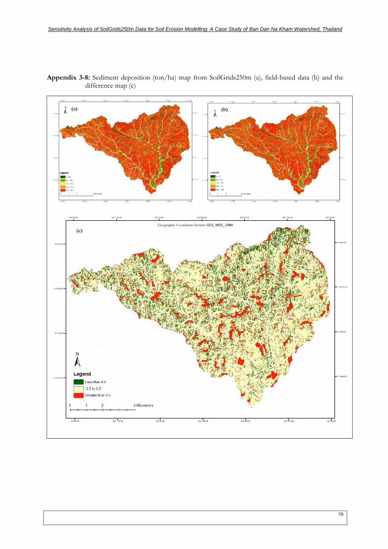
(b) and the difference map (c) ........................................................................................................ 78 Appendix 3-8: Sediment deposition (ton/ha) map from SoilGrids250m (a), field-based data (b) and

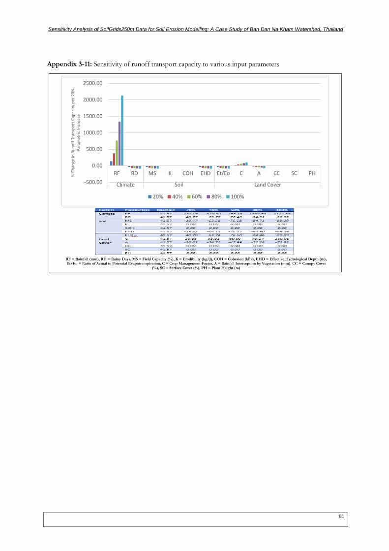
the difference map (c) ...................................................................................................................... 79 Appendix 3-9: Sensitivity of detachment by raindrops various input parameters .................................. 80 Appendix 3-10: Sensitivity of detachment by runoff to various input parameters ................................ 80 Appendix 3-11: Sensitivity of runoff transport capacity to various input parameters ........................... 81

vi

LIST OF FIGURES

Figure 2-1: Study area – Ban Dan Na Kham watershed ........................................................................................ 4

Figure 2-2: Soil map of the study area ....................................................................................................................... 5

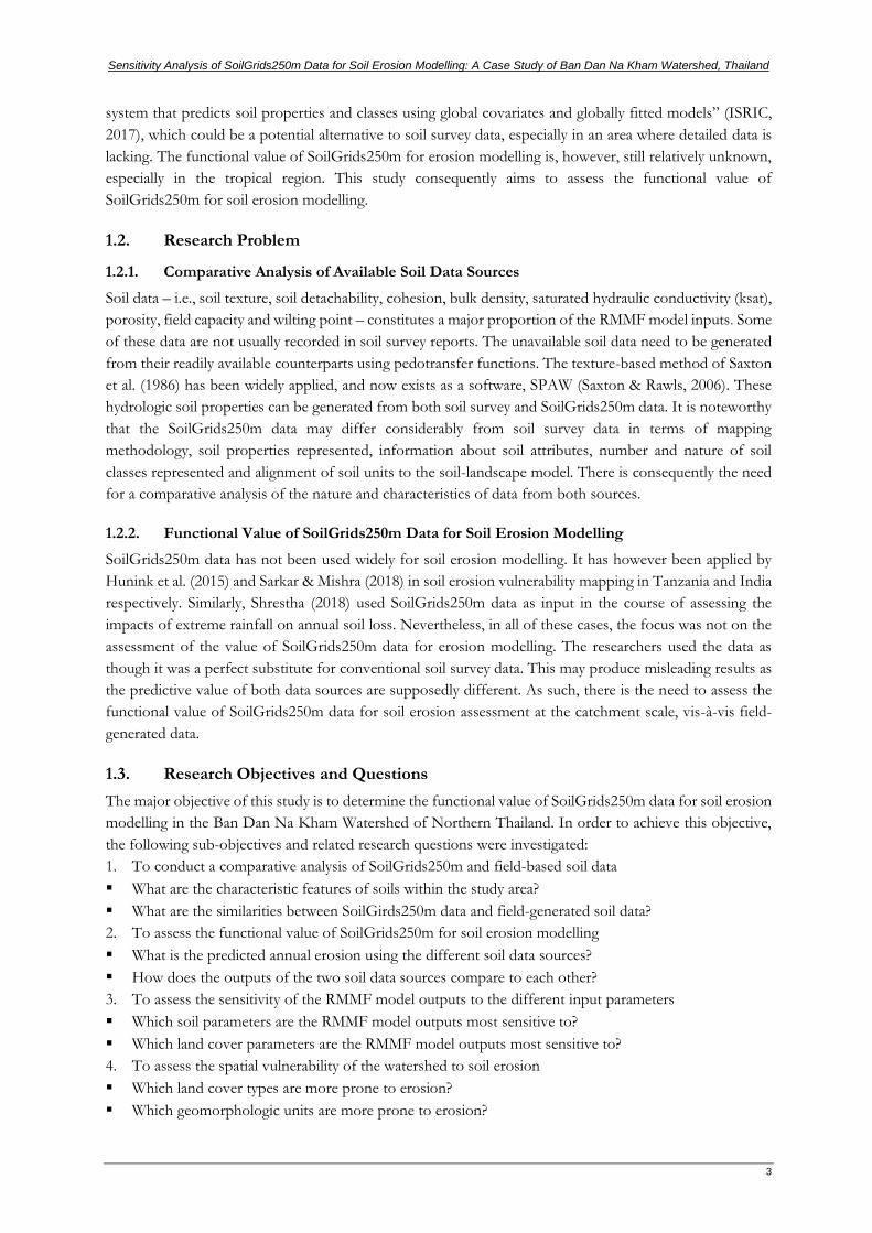
Figure 2-3: Hillslope model ......................................................................................................................................... 6

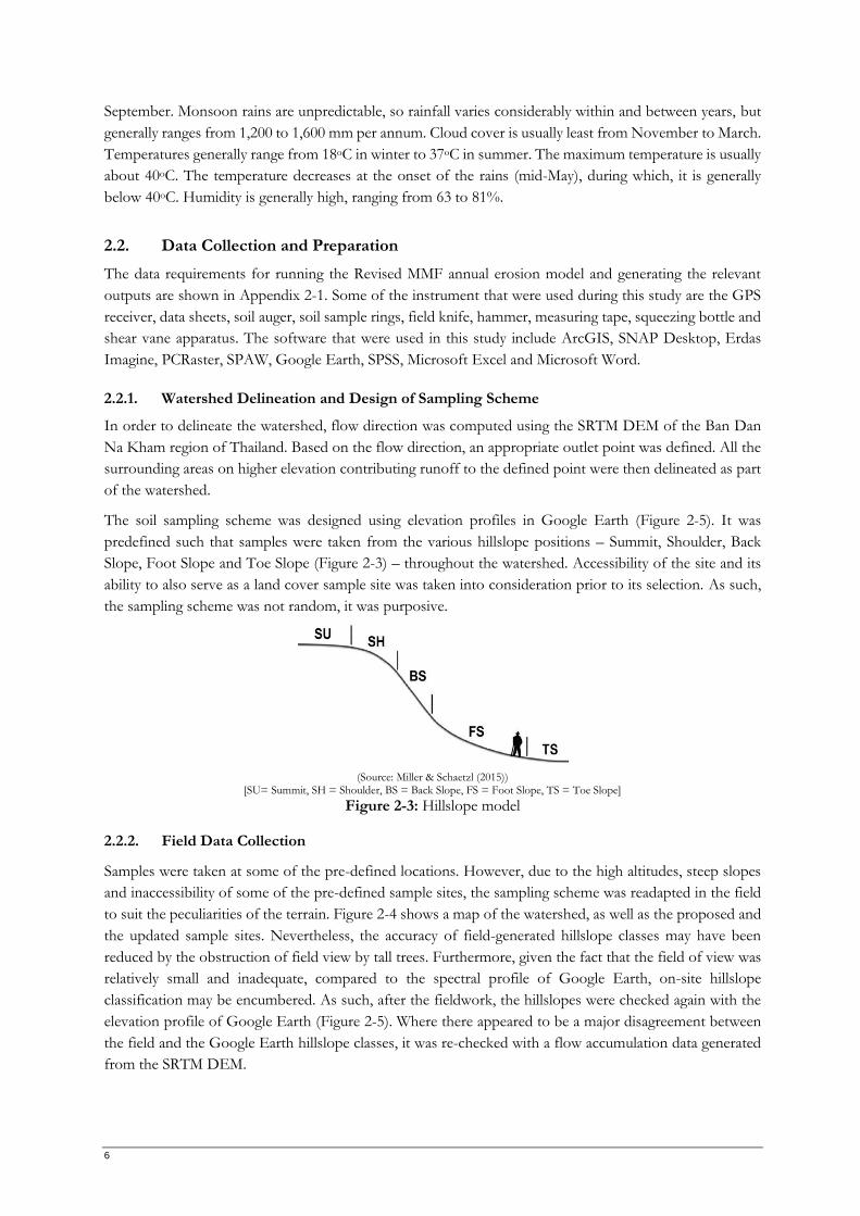
Figure 2-4: Map of the watershed, showing the soil and land cover sample sites .............................................. 7

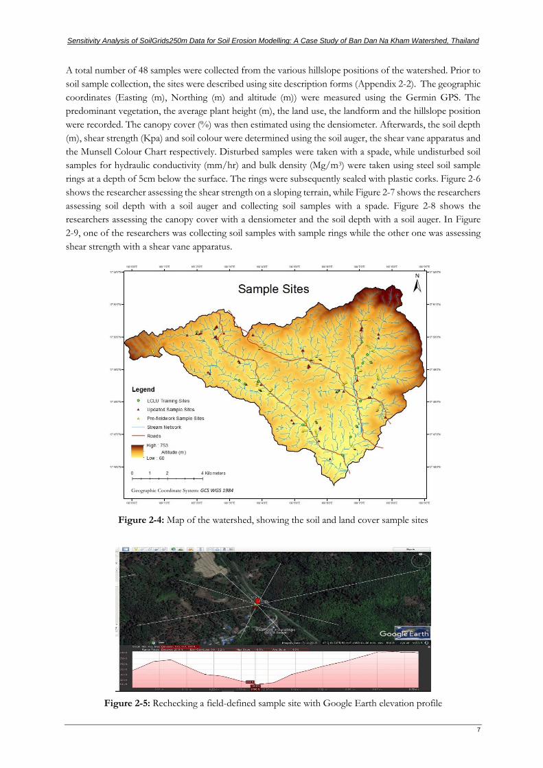
Figure 2-5: Rechecking a field-defined sample site with Google Earth elevation profile ................................. 7

Figure 2-6: Assessment of shear strength on a sloping terrain .............................................................................. 8

Figure 2-7: Sample collection with a spade and assessment of soil depth with a soil auger ............................. 8

Figure 2-8: Assessment of canopy cover with a densiometer and soil depth with a soil auger ........................ 8

Figure 2-9: Sample collection with sample rings and shear strength assessment of level land ......................... 8

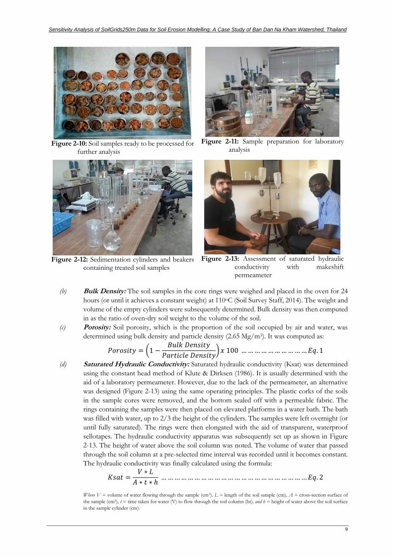
Figure 2-10: Soil samples ready to be processed for further analysis ................................................................... 9

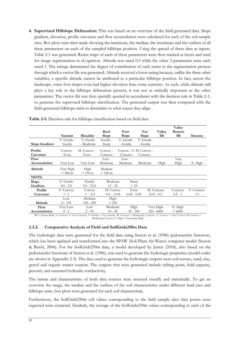
Figure 2-11: Sample preparation for laboratory analysis ......................................................................................... 9

Figure 2-12: Sedimentation cylinders and beakers containing treated soil samples ........................................... 9

Figure 2-13: Assessment of saturated hydraulic conductivity with makeshift permeameter ............................ 9

Figure 2-14: Decision tree for generating the digital hillslope positions ............................................................ 10

Figure 2-15: Landscape patterns represented as geomorphons ........................................................................... 11

Figure 2-16: Cumulative monthly rainfall (mm) in Uttaradit, Thailand (2017/2018) ...................................... 14

Figure 2-17: Flowchart of methods .......................................................................................................................... 18

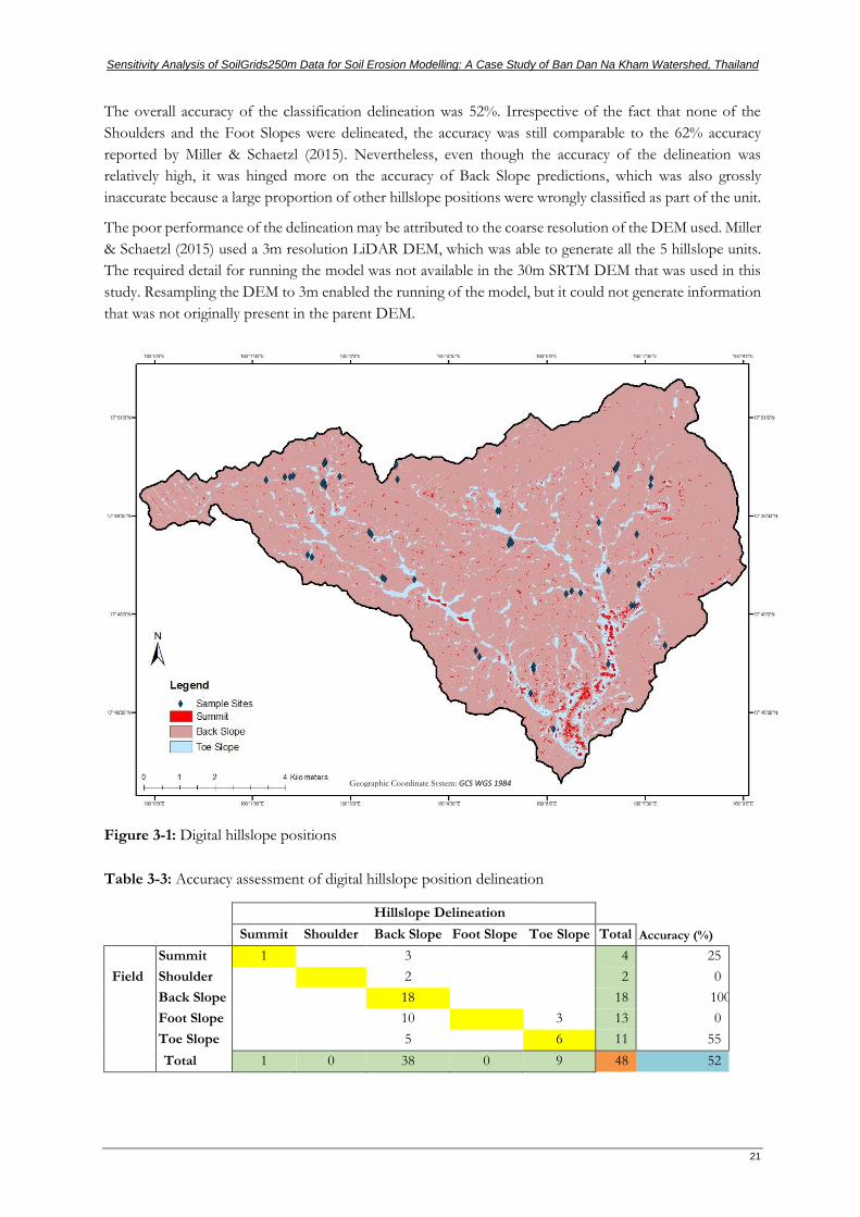
Figure 3-1: Digital hillslope positions ...................................................................................................................... 21

Figure 3-2: Geomorphic units ................................................................................................................................... 22

Figure 3-3: TPI slope units ........................................................................................................................................ 23

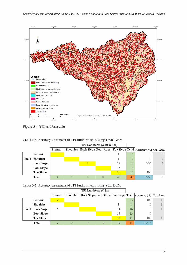
Figure 3-4: TPI landform units ................................................................................................................................. 25

Figure 3-5: Grid cells showing the interactive effects of cell size and arbitrary radius on the generation of

the TPI landform .......................................................................................................................................... 26

Figure 3-6: Variation in flow accumulation (a), elevation (b), profile curvature (c) and slope (d) across the

sample sites .................................................................................................................................................... 27

Figure 3-7: Geomorphic map units for characterizing soil variation across the watershed ............................ 28

Figure 3-8: Spatial variability of sand (a), silt (b), clay (c) and bulk density (d) across the study area ........... 30

Figure 3-9: Spatial variability of soil porosity (a), shear strength (b), saturated hydraulic conductivity (c),

soil organic matter (d), field capacity (e) and wilting point (f) across the study area ......................... 31

Figure 3-10: Spatial variability of organic matter (a), sand (b), silt (c), clay (d), bulk density (e) and shear

strength (f) in the soils underlying the various land cover types of the study area ............................ 33

Figure 3-11: Spatial variability of soil porosity (a), field capacity (b), wilting point (c) and saturated

hydraulic conductivity (d) in the soils underlying the various land cover types of the study area .. 34

Figure 3-12: Comparative point-based assessment of sand (a), silt (b), clay (c), bulk density (d) and organic

matter (e) from field-based and SoilGrids250m data ............................................................................. 36

Figure 3-13: Comparative parcel-based assessment of sand (a), silt (b), clay (c), bulk density (d) and organic

matter (e) from field-based and SoilGrids250m data ............................................................................. 38

Figure 3-14: Land use / land cover map of the Ban Dan Na Kham Watershed .............................................. 39

Figure 3-15: Soil erosion (ton/ha) map from SoilGrids250m (a), field-based data (b) and the difference

map (c) ........................................................................................................................................................... 42

Figure 3-16: Comparative assessment of point-based detachment by raindrops (a), detachment by runoff

(b), total detachment (c), runoff transport capacity (d), sediment deposition (e) and soil erosion (f)

from SoilGrids250m and field-based soil data ........................................................................................ 43


vii

Figure 3-17: Regression analysis of point-based detachment by raindrops [kg/m2] (a), detachment by

runoff [kg/m2] (b), total detachment [ton/ha] (c), runoff transport capacity [kg/m2] (d), sediment

deposition [ton/ha] (e) and soil erosion [ton/ha] (f) from SoilGrids250m and field-based soil data

........................................................................................................................................................................ 44

Figure 3-18: Comparative assessment of parcel-based detachment by raindrops (a), detachment by runoff

(b), total detachment (c), runoff transport capacity (d), sediment deposition (e) and soil erosion (f)

from SoilGrids250m and field-based soil data ........................................................................................ 46

Figure 3-19: Sensitivity of total soil detachment to various input parameters .................................................. 49

Figure 3-20: Sensitivity of runoff estimate to various input parameters............................................................ 50

Figure 3-21: Sensitivity of sediment deposition to various input parameters ................................................... 50

Figure 3-22: Sensitivity of soil loss estimation to various input parameters ..................................................... 51

Figure 3-23: Detachment, deposition and soil loss under different slope conditions ..................................... 52

Figure 3-24: Detachment, deposition and soil loss across different hillslope units ......................................... 53

Figure 3-25: Detachment, deposition and soil loss under different land use types ......................................... 53

Figure 3-26: Map of the watershed showing the different land use types and their respective slope classes

........................................................................................................................................................................ 55

Figure 3-27: Soil erosion (ton/ha) on different land cover-slope units ............................................................. 56

viii

LIST OF TABLES

Table 2-1: Decision rule for hillslope classification based on field data ............................................................. 12

Table 2-2: Baseline settings for sensitivity analysis of model parameters .......................................................... 17

Table 3-1: Variability of soil properties from SoilGrids250m across different hillslope positions ................ 19

Table 3-2: Accuracy assessment of field-generated hillslope units ...................................................................... 20

Table 3-3: Accuracy assessment of digital hillslope position delineation ........................................................... 21

Table 3-4: Accuracy assessment of geomorphic units ........................................................................................... 23

Table 3-5: Accuracy assessment of TPI slope units .............................................................................................. 24

Table 3-6: Accuracy assessment of TPI landform units using a 30m DEM ..................................................... 25

Table 3-7: Accuracy assessment of TPI landform units using a 5m DEM ....................................................... 25

Table 3-8: Accuracy assessment of supervised hillslope delineation .................................................................. 28

Table 3-9: Point-based comparative statistics of the soil datasets ....................................................................... 35

Table 3-10: Parcel-based comparative statistics of the soil datasets ................................................................... 37

Table 3-11: Accuracy assessment report for land use / land cover classification............................................. 40

Table 3-12: Accuracy assessment report for land use / land cover classification (without teak plantation) 40

Table 3-13: Attributes generated for each land cover type ................................................................................... 40

Table 3-14: Point-based comparative statistics for RMMF model outputs ....................................................... 45

Table 3-15: Hillslope parcel-based comparative statistics for RMMF model outputs ..................................... 47

Table 3-16: Soil erosion processes in the different landscape units of the watershed ..................................... 55


1

1. INTRODUCTION

1.1. Background and Justification

Globally, soil erosion has been identified as one of the most destructive and severe forms of land degradation

(FAO & ITPS, 2015; Melaku et al., 2018). This is more so, as the impacts of soil erosion are not limited to

the on-site loss of topsoil, nutrients, organic matter, crop residues, soil quality and growing plants. The off-

site impacts, leading to the inundation of downhill farms by eroded soils, silting in of drainage channels and

reservoirs, water pollution and the degradation aquatic habitat, may even be more critical. Soil erosion

consequently poses a threat to the sustainability of a nation’s economic, social and environmental systems.

The situation is made more precarious by the expectation that climate change will aggravate the current state

of land degradation (Starkloff & Stolte, 2014; Deelstra, 2015; Li & Fang, 2016; Giang et al., 2017; Wang et

al., 2018).

The all-encompassing negative impacts of soil erosion necessitate the need for sustainable land management

that takes erosion control and prevention into consideration. Various preventive and control measures exist,

but the successful implementation of these measures and the attendant land use planning requires a prior

understanding of the spatio-temporal dynamics of soil degradation in a region. As a consequence, proper

land use planning at the watershed scale requires the use of state-of-the-art erosion prediction models (De

Vente et al., 2013). Many soil erosion prediction models are currently in existence (Hajigholizadeh et al.,

2018). These models may either be data-driven or process-driven, but they are generally grouped into event-

based, daily and annual models, depending on the temporal resolution of the required rainfall data.

Event-based models focus on the relatively short duration, high intensity rainfall and runoff events that

account for the bulk of the soil erosion that take place on an annual basis. Numerous event-based models

are currently in existence, some of which are the Limburg Soil Erosion Model [LISEM] (De Roo et al.,

1996), the Areal Nonpoint Source Watershed Environment Response Simulation [ANSWERS] (Beasley et

al., 1980), the Kinematic Runoff and Erosion Model [KINEROS] (Woolhiser et al., 1990) and the European

Soil Erosion Model [EUROSEM] (Morgan et al., 1998). According to Hajigholizadeh et al. ( 2018), all of

these models are catchment-based, generate a wide range of hydrological outputs, and require event-based

rainfall data. It is, however, noteworthy that not all event-based models require detailed short duration

rainfall data. LandscApe ProcesS modelling at mUlti-dimensions and Scales [LAPSUS] (Schoorl et al., 2000;

Sonneveld et al., 2010), unlike most other event-based models, considers the total rainfall of one year as a

single rainfall event. This is hinged on the fact that, while other event-based models are designed for the

assessment of the degree of land degradation caused by a single rainfall event, LAPSUS was designed for

the assessment of how the landscape has evolved over a long period of time. As such, the kind of

information required, determines, to a large extent, the temporal resolution of the required rainfall data, and

consequently, the kind of model adopted.

The inherent processes of a typical event-based model like LISEM, are divided into the hydrological and

the sediment cycle (De Roo et al., 1996; Jetten, 2018). The hydrological cycle encompasses such processes

as rainfall, interception, storage, kinematic wave, flooding and coupling of flow; while the sediment cycle,

on the other hand, is made up of such processes as splash detachment, flow detachment, deposition,

sediment transport, sediment diffusion and sediment load (Jetten, 2018a). In line with the contention of

Starkloff & Stolte (2014), these models are consequently essential to the understanding of the underlying

processes behind rainfall, interception, splash, runoff, surface storage, erosion and deposition; providing us

with the insight on how to effectively combat the negative impacts of extreme weather events.

2

Furthermore, as Hajigholizadeh et al. (2018) asserted, event-based hydrological models are appropriate for

regions with strongly seasonal rainfall, where the bulk of the soil erosion would be associated with high

intensity rainfall events. This is in line with the findings of other researchers who assessed the relationship

between rainfall intensity and the magnitude of erosion that take place within a watershed (Baartman et al.,

2012; Alexakis et al., 2013; Clutario et al., 2014; Mohamadi & Kavian, 2015; Wang et al., 2016). Moreover,

Baartman et al. (2012) and Shrestha & Jetten (2018) concluded that the best estimate of annual soil erosion

should be the sum of all the event-based erosion estimate for the year. Theoretically, this may be feasible,

but it is easier and more realistic to compute annual soil loss as the sum of the daily soil loss that took place

in a single year.

More so, the event-based models need a lot of data because, in addition to simulating particle detachment,

transportation and deposition during an event in detail, it is required that the catchment needs to be

initialized to simulate the circumstances before the rainfall event (Shrestha & Jetten, 2018). The situation is

made dire by the fact that the detailed, high temporal and spatial resolution rainfall data required for event-

based rainfall-runoff modelling is not available in most developing countries. In the absence of the

appropriate data, daily rainfall-runoff modelling for erosion estimates is a good approximation of event-

based model outputs on a daily basis (Shrestha & Jetten, 2018). Rainfall data is, however, not the only input

data required to run an erosion model. The models require detailed input of soil, climate, land cover and

topographic data, most of which are not readily accessible. These data, according to Näschen et al. (2018),

are rarely available in many developing countries, constituting a major drawback to the use of physically-

based models. Similarly, Avwunudiogba & Hudson (2014) contended that the less stringent data

requirements and ease of implementation of lumped parameter annual hydrologic models make them the

preferred choice in humid tropical mountainous environment.

Indeed, annual soil erosion models are less data-intensive, consequently making them more amenable to use

in many developing countries, where scarcity of good quality, high resolution data is a major issue. Annual

models are based on the average annual rainfall, and as such, according to Hajigholizadeh et al. (2018), may

not be appropriate for regions with strongly seasonal rainfall events. This is a major challenge, but when

projections are required on the spatial extent of land degradation, as well as the impacts on policy decisions

relating to different land uses, annual hydrological models are still quite useful. In spite of that, the available

models have many limitations.

Most annual lumped parameter models, like Universal Soil Loss Equation [USLE] (Wischmeier & Smith,

1978; Renard et al., 1991) and Soil Loss Estimator Model for Southern Africa [SLEMSA] (Stocking, 1981)

are incapable of quantifying sediment deposition and runoff (Avwunudiogba & Hudson, 2014). This limits

the range of applicability of these models in landscape, catchment and watershed management. Revised

Morgan-Morgan-Finney (RMMF) Model, unlike these models, can be used to estimate a wide range of

hydrological processes like sediment detachment by runoff and raindrops, total sediment detachment,

runoff, runoff transport capacity, sediment deposition and soil loss (Morgan, 2001). This makes it a veritable

tool for land resources management as it effectively combines relatively low data needs with the generation

of outputs with a wide range of usefulness.

Despite the relatively low data requirements of the RMMF model, it still requires input of soil, climate, land

cover and topographic data. Nonetheless, while land cover and topographic data can be generated from

satellite imageries and digital elevation models (DEM) respectively, accessibility of soil data is more

problematic. This makes the acquisition of sound soil information critical and inevitable (Schuler et al.,

2006), underscoring the need for up-to-date location-specific soil information. Conventional soil surveys are

however, expensive, subjective and time-consuming (Moonjun, 2007; Schuler et al., 2006), buttressing the

need for cheaper, systematic and readily-available soil data. Recently a freely available SoilGrids data

(https://soilgrids.org/) became available at 250m spatial resolution. It is “a globally consistent, data-driven


3

system that predicts soil properties and classes using global covariates and globally fitted models” (ISRIC,

2017), which could be a potential alternative to soil survey data, especially in an area where detailed data is

lacking. The functional value of SoilGrids250m for erosion modelling is, however, still relatively unknown,

especially in the tropical region. This study consequently aims to assess the functional value of

SoilGrids250m for soil erosion modelling.

1.2. Research Problem

1.2.1. Comparative Analysis of Available Soil Data Sources

Soil data – i.e., soil texture, soil detachability, cohesion, bulk density, saturated hydraulic conductivity (ksat),

porosity, field capacity and wilting point – constitutes a major proportion of the RMMF model inputs. Some

of these data are not usually recorded in soil survey reports. The unavailable soil data need to be generated

from their readily available counterparts using pedotransfer functions. The texture-based method of Saxton

et al. (1986) has been widely applied, and now exists as a software, SPAW (Saxton & Rawls, 2006). These

hydrologic soil properties can be generated from both soil survey and SoilGrids250m data. It is noteworthy

that the SoilGrids250m data may differ considerably from soil survey data in terms of mapping

methodology, soil properties represented, information about soil attributes, number and nature of soil

classes represented and alignment of soil units to the soil-landscape model. There is consequently the need

for a comparative analysis of the nature and characteristics of data from both sources.

1.2.2. Functional Value of SoilGrids250m Data for Soil Erosion Modelling

SoilGrids250m data has not been used widely for soil erosion modelling. It has however been applied by

Hunink et al. (2015) and Sarkar & Mishra (2018) in soil erosion vulnerability mapping in Tanzania and India

respectively. Similarly, Shrestha (2018) used SoilGrids250m data as input in the course of assessing the

impacts of extreme rainfall on annual soil loss. Nevertheless, in all of these cases, the focus was not on the

assessment of the value of SoilGrids250m data for erosion modelling. The researchers used the data as

though it was a perfect substitute for conventional soil survey data. This may produce misleading results as

the predictive value of both data sources are supposedly different. As such, there is the need to assess the

functional value of SoilGrids250m data for soil erosion assessment at the catchment scale, vis-à-vis field-

generated data.

1.3. Research Objectives and Questions

The major objective of this study is to determine the functional value of SoilGrids250m data for soil erosion

modelling in the Ban Dan Na Kham Watershed of Northern Thailand. In order to achieve this objective,

the following sub-objectives and related research questions were investigated:

1. To conduct a comparative analysis of SoilGrids250m and field-based soil data

▪ What are the characteristic features of soils within the study area?

▪ What are the similarities between SoilGirds250m data and field-generated soil data?

2. To assess the functional value of SoilGrids250m for soil erosion modelling

▪ What is the predicted annual erosion using the different soil data sources?

▪ How does the outputs of the two soil data sources compare to each other?

3. To assess the sensitivity of the RMMF model outputs to the different input parameters

▪ Which soil parameters are the RMMF model outputs most sensitive to?

▪ Which land cover parameters are the RMMF model outputs most sensitive to?

4. To assess the spatial vulnerability of the watershed to soil erosion

▪ Which land cover types are more prone to erosion?

▪ Which geomorphologic units are more prone to erosion?

4

2. METHODOLOGY

2.1. Study Area

2.1.1. Location of the Study Area

This study was carried out at the Ban Dan Na Kham Watershed located in Mueang District, Uttaradit

Province, Thailand. It is located within Latitudes 17o40’N – 17o55’N, and Longitudes 99o50’E – 100o20’E.

It covers an area of approximately 86.91 km2, with altitude ranging from 60 to 753m above sea level. It is

about 489 km away from Bangkok and 123 km from Phitsanulok. It is accessible by road and by train to

Phitsanulok, Bangkok and other neighbouring cities. The location map of the study area is shown in Figure

2-1.

Figure 2-1: Study area – Ban Dan Na Kham watershed

2.1.2. Topography and Hydrology

The region is located in the Northern Continental Highlands (Scholten & Siriphant, 1973). It is hilly and

mountainous; is the source of several rivers and streams, and it is located within the vicinity of the Nan

River. The hills are north-south oriented, are parallel from west to east, and are intersected by several valleys.

The southern fringe is dominated by high terraces and fans of old alluvium and colluvium. The landscape is

essentially an undulating terrain.

2.1.3. Geology and Soils

There are three groups of soils in the study area, viz. soils of hills and mountains, soils of the higher terraces

and low plateaus, and soils of alluvial plains and lower terraces (Figure 2-2). Nevertheless, due to the very

Geographic Coordinate System: GCS WGS 1984


5

coarse scale (1: 2,500,000) of the soil map (Figure 2-2), the only soil unit that falls within the watershed is

the reddish-yellow podzolic soils on steep lands formed from acid to intermediate rocks (Figure 2-2). The

soil units within the area, as summarized in the map produced by Moormann and Rojanasoontan in 1967

and stored in the European digital archive on soil maps (EuDASM) (Panagos et al., 2011), are outlined

below.

a. Soils of Hills and Mountains: The soils are divided into four classes:

• Red-yellow podzolic soils, mostly on hilly terrain, formed on materials from acid and intermediate rocks

(Class 16)

• Red-yellow podzolic soils and reddish-brown lateritic soils found on steep land rich in intermediate

basic rocks (Class 20).

• Mainly red-yellow podzolic soils formed on steep lands rich in acid to intermediate rocks (Class 21)

• Shallow undifferentiated soils on lava plateaus and volcanoes (Class 23)

b. Soils of the Higher Terraces and Low Plateaus: The soils are divided into two classes:

• Gray podzolic soils on old alluvium (Class 14)

• Red-yellow podzolic soils on old alluvium (Class15)

c. Soils of Alluvial Plains and Lower Terraces: The soils are divided into three classes:

• Alluvial soils on recent fresh water alluvium (Class 2)

• Low humic gley soils on semi-recent and old alluvium (Class 7)

• Low humic gley soils and gray or reddish yellow podzolic soils on old alluvium (Class 9)

2.1.4. Climate

Ban Dan Na Kham Watershed is located in the humid tropics, under the influence of the north-eastern and

south-western Monsoons. It has three seasons: dry (Winter), hot (Summer, with gradually increasing rainfall

and thunderstorms) and rainy seasons. Over 90 % of the annual rains fall within the rainy season, which

lasts for about 5 months (mid-May to mid-October), with most of the rains coming in August and

(Source: General Soil Condition of Thailand by produced by Moormann and Rojanasoontan in 1967 and stored in the EuDASM Archive (Panagos et al., 2011)

Figure 2-2: Soil map of the study area


6

September. Monsoon rains are unpredictable, so rainfall varies considerably within and between years, but

generally ranges from 1,200 to 1,600 mm per annum. Cloud cover is usually least from November to March.

Temperatures generally range from 18oC in winter to 37oC in summer. The maximum temperature is usually

about 40oC. The temperature decreases at the onset of the rains (mid-May), during which, it is generally

below 40oC. Humidity is generally high, ranging from 63 to 81%.

2.2. Data Collection and Preparation

The data requirements for running the Revised MMF annual erosion model and generating the relevant

outputs are shown in Appendix 2-1. Some of the instrument that were used during this study are the GPS

receiver, data sheets, soil auger, soil sample rings, field knife, hammer, measuring tape, squeezing bottle and

shear vane apparatus. The software that were used in this study include ArcGIS, SNAP Desktop, Erdas

Imagine, PCRaster, SPAW, Google Earth, SPSS, Microsoft Excel and Microsoft Word.

2.2.1. Watershed Delineation and Design of Sampling Scheme

In order to delineate the watershed, flow direction was computed using the SRTM DEM of the Ban Dan

Na Kham region of Thailand. Based on the flow direction, an appropriate outlet point was defined. All the

surrounding areas on higher elevation contributing runoff to the defined point were then delineated as part

of the watershed.

The soil sampling scheme was designed using elevation profiles in Google Earth (Figure 2-5). It was

predefined such that samples were taken from the various hillslope positions – Summit, Shoulder, Back

Slope, Foot Slope and Toe Slope (Figure 2-3) – throughout the watershed. Accessibility of the site and its

ability to also serve as a land cover sample site was taken into consideration prior to its selection. As such,

the sampling scheme was not random, it was purposive.

(Source: Miller & Schaetzl (2015))

[SU= Summit, SH = Shoulder, BS = Back Slope, FS = Foot Slope, TS = Toe Slope]

Figure 2-3: Hillslope model

2.2.2. Field Data Collection

Samples were taken at some of the pre-defined locations. However, due to the high altitudes, steep slopes

and inaccessibility of some of the pre-defined sample sites, the sampling scheme was readapted in the field

to suit the peculiarities of the terrain. Figure 2-4 shows a map of the watershed, as well as the proposed and

the updated sample sites. Nevertheless, the accuracy of field-generated hillslope classes may have been

reduced by the obstruction of field view by tall trees. Furthermore, given the fact that the field of view was

relatively small and inadequate, compared to the spectral profile of Google Earth, on-site hillslope

classification may be encumbered. As such, after the fieldwork, the hillslopes were checked again with the

elevation profile of Google Earth (Figure 2-5). Where there appeared to be a major disagreement between

the field and the Google Earth hillslope classes, it was re-checked with a flow accumulation data generated

from the SRTM DEM.


7

A total number of 48 samples were collected from the various hillslope positions of the watershed. Prior to

soil sample collection, the sites were described using site description forms (Appendix 2-2). The geographic

coordinates (Easting (m), Northing (m) and altitude (m)) were measured using the Germin GPS. The

predominant vegetation, the average plant height (m), the land use, the landform and the hillslope position

were recorded. The canopy cover (%) was then estimated using the densiometer. Afterwards, the soil depth

(m), shear strength (Kpa) and soil colour were determined using the soil auger, the shear vane apparatus and

the Munsell Colour Chart respectively. Disturbed samples were taken with a spade, while undisturbed soil

samples for hydraulic conductivity (mm/hr) and bulk density (Mg/m3) were taken using steel soil sample

rings at a depth of 5cm below the surface. The rings were subsequently sealed with plastic corks. Figure 2-6

shows the researcher assessing the shear strength on a sloping terrain, while Figure 2-7 shows the researchers

assessing soil depth with a soil auger and collecting soil samples with a spade. Figure 2-8 shows the

researchers assessing the canopy cover with a densiometer and the soil depth with a soil auger. In Figure

2-9, one of the researchers was collecting soil samples with sample rings while the other one was assessing

shear strength with a shear vane apparatus.

Figure 2-4: Map of the watershed, showing the soil and land cover sample sites

Figure 2-5: Rechecking a field-defined sample site with Google Earth elevation profile


8

Figure 2-6: Assessment of shear strength on a

sloping terrain

Figure 2-7: Sample collection with a spade and

assessment of soil depth with a soil auger

Figure 2-8: Assessment of canopy cover with a

densiometer and soil depth with a soil auger

Figure 2-9: Sample collection with sample rings

and shear strength assessment of level land

2.2.3. Soil Analysis

The 48 soil samples collected in the field were analysed at the Civil Engineering Laboratory of the Naresuan

University in Phitsanulok, Thailand. The undisturbed samples were tested for saturated hydraulic

conductivity, bulk density and porosity. The disturbed samples were tested for particle size distribution, soil

texture and organic matter content. Figure 2-10 shows the soil samples in metal cans while Figure 2-11

shows the researchers preparing the soil samples for analysis.

(a) Particle Size Distribution: The particle size distribution was assessed using the hydrometer

method, as described in the Soil Survey and Laboratory Manual (Soil Survey Staff, 2014). The

soil samples were air-dried and passed through a 2mm sieve. 40g of the sample was weighed

into a glass beaker to which 100ml of distilled water and 100ml of Calgon (5% sodium

hexametaphosphate) solution were added. It was then left overnight, after which it was passed

into a dispersing cup and stirred for 5 minutes with a mechanical mixer. The mixture was

transferred into a 1000ml sedimentation cylinder, which was then filled to the 1000ml mark.

Another sedimentation cylinder containing 100ml Calgon and distilled water, but no soil, was

also prepared. The soil solution was stirred for 30 seconds. The temperature of both solutions

were recorded, and the hydrometer readings taken at 30 seconds, 60 seconds, 3 minutes, 10

minutes, 30 minutes, 60 minutes, 90 minutes, 120 minutes and 1440 minutes. 10g of the soils

were subsequently oven-dried at 105oC, and then, reweighed. The proportion of sand, silt and

clay in the soil were then computed as suggested by Gee & Bauder (1986) and described by Soil

Survey Staff (2014). Using the proportions, the soil texture was determined with the textural

triangle. Figure 2-12 shows the sedimentation cylinders and beakers containing soil samples

already treated with sodium hexametaphosphate.


9

Figure 2-10: Soil samples ready to be processed for

further analysis

Figure 2-11: Sample preparation for laboratory

analysis

Figure 2-12: Sedimentation cylinders and beakers

containing treated soil samples

Figure 2-13: Assessment of saturated hydraulic

conductivity with makeshift permeameter

(b) Bulk Density: The soil samples in the core rings were weighed and placed in the oven for 24

hours (or until it achieves a constant weight) at 110oC (Soil Survey Staff, 2014). The weight and

volume of the empty cylinders were subsequently determined. Bulk density was then computed

in as the ratio of oven-dry soil weight to the volume of the soil.

(c) Porosity: Soil porosity, which is the proportion of the soil occupied by air and water, was

determined using bulk density and particle density (2.65 Mg/m3). It was computed as:

𝑃𝑜𝑟𝑜𝑠𝑖𝑡𝑦 = (1 −𝐵𝑢𝑙𝑘 𝐷𝑒𝑛𝑠𝑖𝑡𝑦

𝑃𝑎𝑟𝑡𝑖𝑐𝑙𝑒 𝐷𝑒𝑛𝑠𝑖𝑡𝑦) 𝑥 100 … … … … … … … … … … 𝐸𝑞. 1

(d) Saturated Hydraulic Conductivity: Saturated hydraulic conductivity (Ksat) was determined

using the constant head method of Klute & Dirksen (1986). It is usually determined with the

aid of a laboratory permeameter. However, due to the lack of the permeameter, an alternative

was designed (Figure 2-13) using the same operating principles. The plastic corks of the soils

in the sample cores were removed, and the bottom sealed off with a permeable fabric. The

rings containing the samples were then placed on elevated platforms in a water bath. The bath

was filled with water, up to 2/3 the height of the cylinders. The samples were left overnight (or

until fully saturated). The rings were then elongated with the aid of transparent, waterproof

sellotapes. The hydraulic conductivity apparatus was subsequently set up as shown in Figure

2-13. The height of water above the soil column was noted. The volume of water that passed

through the soil column at a pre-selected time interval was recorded until it becomes constant.

The hydraulic conductivity was finally calculated using the formula:

𝐾𝑠𝑎𝑡 =𝑉 ∗ 𝐿

𝐴 ∗ 𝑡 ∗ ℎ … … … … … … … … … … … … … … … … … … … … … … 𝐸𝑞. 2

Where V = volume of water flowing through the sample (cm3), L = length of the soil sample (cm), A = cross-section surface of

the sample (cm2), t = time taken for water (V) to flow through the soil column (hr), and h = height of water above the soil surface

in the sample cylinder (cm).

10

(e) Soil Organic Matter: Organic matter was estimated through the direct method of loss on

ignition as reported by Dor & Banin (1989). 5g of soil was weighed into a crucible and left

overnight in an oven set at a temperature of 105oC. It was then cooled to room temperature in

a desiccator for 20 minutes, after which it was reweighed and transferred to a furnace. The

temperature of the furnace was raised to 400oC. The sample was left in the furnace for 8 hours.

It was then removed, and again cooled to room temperature in a desiccator, before being

reweighed. The organic matter was expressed as a percentage of the weight loss between oven-

drying and furnace ignition to the weight after oven-drying.

2.3. Comparative Analysis of SoilGrids250m and Field Data

Soil data was generated from two sources, viz. SoilGrids250m and field sampling. The 5cm layer of the

SoilGrids250m data for the study area was downloaded from https://soilgrids.org/. Bulk density, organic

carbon, clay, sand, silt and gravel data were available in this repository for 7 soil depth intervals (ISRIC,

2017). The field samples were collected from various hillslope positions (Figure 2-3). These were, however,

point data that need to be extrapolated for the entire watershed. Several hillslope algorithms were considered

as potential tools for the delineation of the soil units. These include the digital hillslope classification

described by Miller & Schaetzl (2015), the r.geomorphon algorithm in GRASS GIS based on the works of

Jasiewicz & Stepinski (2013), the TPI (topographic position index) slope and landform classification

implemented by Miller (2014), but based on the works of Deumlich et al. (2010) and the supervised hillslope

classification which was based on an overview of the field-generated data.

2.3.1. Generation of Physiographic Map for Representing Soil Variation

Several hillslope delineation algorithms were considered in the course of this study. Each of these are briefly

discussed below.

1. Digital Classification of Hillslope Positions: This was based on the work of Miller & Schaetzl (2015).

They used 3m resolution LiDAR DEMs to generate slope gradient, profile curvature and relative

elevation at a neighbourhood scale of 9m, 63m and 135m respectively. The adopted neighbourhoods

were in line with the analysis scale that soil scientists use while analysing hillslope positions (Miller, 2014).

In this study, to mimic the resolution of the LiDAR DEM, the SRTM DEM was resampled to 3m using

cubic convolution. Slope gradient, profile curvature and relative elevations were then calculated using

the appropriate neighbourhood scales. The slope gradient map was classified into high, medium and low;

profile curvature was classified into positive and negative; while relative elevation was classified into high

and low. The hillslope was then delineated using the decision tree algorithm (Figure 2-14) implemented

in the relief analysis toolbox by Miller (2014). The output generated from the model was then compared

with the field-generated hillslope units to determine to what extent they align.

Source: Miller & Schaetzl (2015)

Figure 2-14: Decision tree for generating the digital hillslope positions

https://soilgrids.org/


11

2. Geomorphic Unit Delineation Using r.geomorphon in GRASS GIS: The geomorphon classifies

hillslopes using pattern recognition, rather than differential geometry (Jasiewicz & Stepinski, 2013). It

creates a pattern by comparing a target pixel with the pixel values of the 8 neighbouring pixels along the

line of sight of the 8 principal directions. This creates a tuple of negatives, positives and zeros, indicating

pixels with lower, higher and equal values respectively. The output however depends on the search radius

and the flatness threshold. The search radius refers to the distance or the number of cells around the

target cell on which the calculation is based, while the flatness threshold relates to degree of flatness of

the area under observation. According to Veselsky et al. (2015), as the flatness threshold increases, the

spatial extent of plains automatically increases at the expense of other landforms. In this way, the model

creates 498 unique patterns for every cell. Nevertheless, out of all of these, only 10 patterns represent

the possible morphological terrain types of a standard landscape, referred to as geomorhons (Figure

2-15). In this study, an outer radius of 45m was adopted since it was not meant to be less than the

resolution of the DEM. Given the mountainous nature of the terrain, the pre-programmed flatness

threshold of 1 and an inner search radius of 0 were used for the generation of the geomorphic units. The

generated units were then compared with the field-generated hillslope units to determine to what extent

they align.

Source: Jasiewicz & Stepinski (2013)

Figure 2-15: Landscape patterns represented as geomorphons

3. TPI Slope and Landform Classification: The TPI (topographic position index) Slope and Landform

Classes were calculated using the Relief Analysis toolbox developed by Miller (2014). The underlying

theory behind the functionality of the computations were based on the works of Deumlich et al. (2010).

They contended that using the TPI slope and landform analysis, information can be combined at both

the local and regional scale, enabling the establishment of relationships that can help in the delineation

of the spatial extent and distribution of soils. The TPI compares the elevation of each grid cell in a DEM

with the mean elevation of a neighbourhood defined by circles of arbitrary radius.

In this study the 30m SRTM DEM was used to generate TPI and slope maps, adopting the 25m, 125m

and 500m neighbourhood settings used by Deumlich et al. (2010). They were then used as inputs for the

calculation of the TPI Landform and TPI Slope Position Classes. Furthermore, the DEMs were

resampled to 5m resolution to mimic the resolution of the airborne laser scanning-derived DEM used

by Deumlich et al. (2010). The process was repeated and the output recalculated. The outputs were then

compared with the field-generated hillslope units to determine to what extent they align.

12

4. Supervised Hillslope Delineation: This was based on an overview of the field-generated data. Slope

gradient, elevation, profile curvature and flow accumulation were calculated for each of the soil sample

sites. Box plots were then made showing the minimum, the median, the maximum and the outliers of all

these parameters on each of the sampled hillslope position. Using the spread of these data as inputs,

Table 2-1 was generated. Raster maps of each of these parameters were then stacked as layers and used

for image segmentation in eCognition. Altitude was rated 0.5 while the other 3 parameters were each

rated 1. The ratings determined the degree of contribution of each raster in the segmentation process

through which a vector file was generated. Altitude received a lower rating because, unlike the three other

variables, a specific altitude cannot be attributed to a particular hillslope position. In fact, across the

landscape, some foot slopes even had higher elevation than some summits. As such, while altitude still

plays a key role in the hillslope delineation process, it was not as critically important as the other

parameters. The vector file was then spatially queried in accordance with the decision rule in Table 2-1,

to generate the supervised hillslope classification. The generated output was then compared with the

field-generated hillslope units to determine to what extent they align.

Table 2-1: Decision rule for hillslope classification based on field data

Summit Shoulder Back Slope

Foot Slope

Toe Slope

Valley SB

Valley Bottom

SB Streams

Slope Gradient V. Gentle -

Gentle V. Gentle

- Moderate Gentle -

Steep V. Gentle - Gentle

V. Gentle - Gentle

Profile Curvature

Convex - Even

M. Convex - Even

Convex - Concave

Convex - V. Concave

M. Convex - Concave

Flow Accumulation Very Low Very Low

Low - Moderate

Low - Moderate Moderate High

Very High E. High

Altitude Very High High Medium

> 180 m > 150 m > 120 m NOTE:

Slope Gradient

V. Gentle Gentle Moderate Steep 0.0 - 5.0 5.0 - 15.0 15 - 23 > 23

Profile Curvature

V. Convex Convex M. Convex Even M. Concave Concave V. Concave

< -1 -1 - -0.5 -0.5 - -0.05 -0.05 - 0.05 0.05 - 0.5 0.5 - 1 >1

Altitude

Low Medium High 0 - 150 150 - 250 > 250

Flow Accumulation

Very Low Low Moderate High Very High E. High 0 - 2 2 - 10 10 - 50 50 - 250 250 - 6000 > 6000

SB = Stream Beds, V. Concave = Very Concave, V. Gentle = Very Gentle, M. Concave = Moderately Concave, V. Convex = Very Convex M. Convex = Moderately Convex, E. High = Extremely High

2.3.2. Comparative Analysis of Field and SoilGrids250m Data

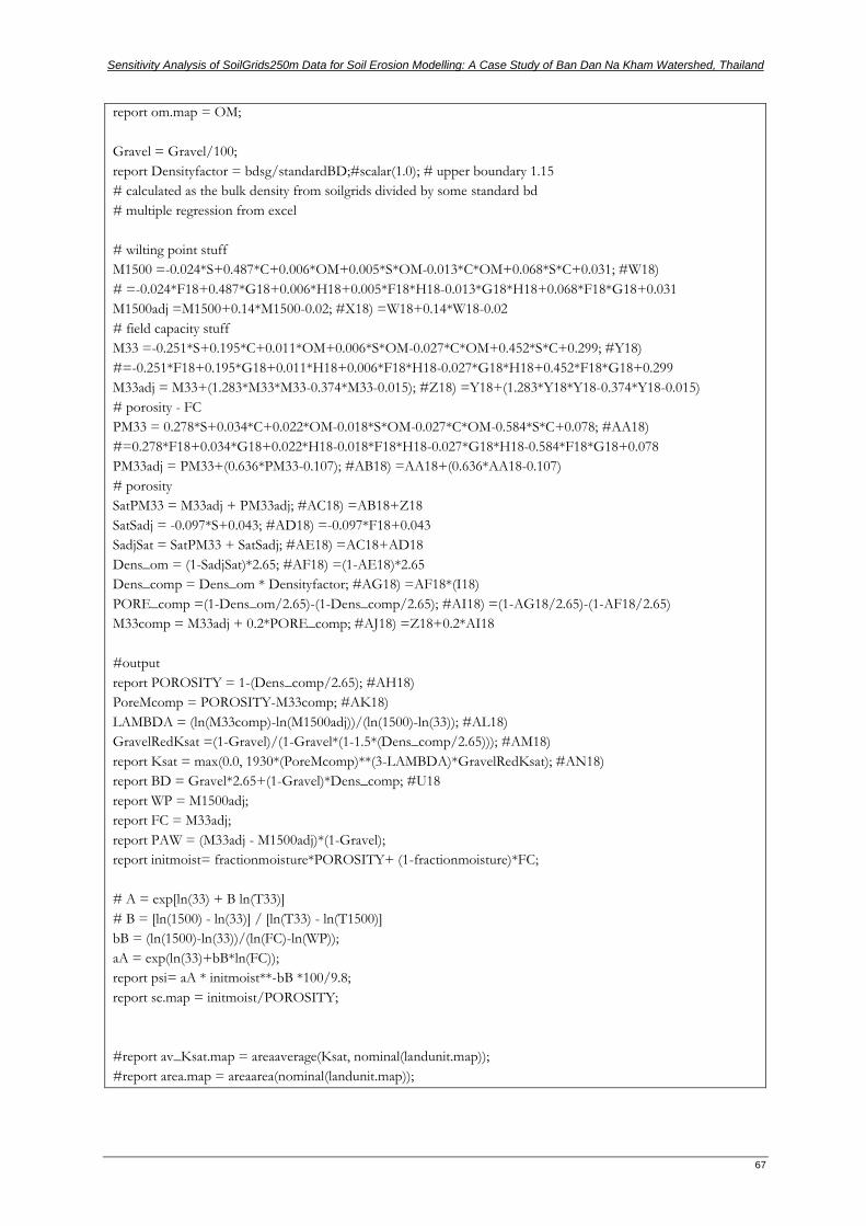
The hydrologic data were generated for the field data using Saxton et al. (1986) pedotransfer functions,

which has been updated and transformed into the SPAW (Soil-Plant-Air-Water) computer model (Saxton

& Rawls, 2006). For the SoilGrids250m data, a model developed by Jetten (2018), also based on the

pedotransfer functions of Saxton et al. (1986), was used to generate the hydrologic properties (model codes

are shown in Appendix 2-3). The data used to generate the hydrologic outputs were soil texture, sand, clay,

gravel and organic matter content. The outputs that were generated include wilting point, field capacity,

porosity and saturated hydraulic conductivity.

The nature and characteristics of both data sources were assessed visually and statistically. To get an

overview the range, the median and the outliers of the soil characteristics under different land uses and

hillslope units, box plots were generated for each soil characteristic.

Furthermore, the SoilGrids250m cell values corresponding to the field sample sites data points were

expected were extracted. Similarly, the average of the SoilGrids250m values corresponding to each of the


13

delineated hillslope units were also calculated. Box plots were then generated for the SoilGrids250m and

field data to visually show how they compare to each other. Regression graphs were also generated to

determine the kind of relationship that exists between the two datasets.

To determine to what extent the data sources are similar, the Euclidean Distance between the two data

sources was computed using the formula:

𝐸𝐷 = √∑(𝑥𝑖 − 𝑦𝑖)2

𝑛

𝑖=1

… … … … … … … … … … … … … … … … … … … … 𝐸𝑞. 3

Where ED = Euclidean Distance, n = number of variables, i = point variable (soil characteristic), x = SoilGrid250m data and y = Field Data.

To determine whether there is a statistically significant difference between the 2 sets of data some

preliminary tests were conducted to determine which statistical methods are more appropriate for the

assessment. Skewness and kurtosis z-values, and Shapiro-Wilk test p-value were calculated to determine

whether the data were normal. The data were considered to be normal if the Shapiro-Wilk test p-value is

greater than 0.05 and the skewness and kurtosis z-values are within the range of -1.96 to +1.96. Levene’s

Test was conducted to determine whether the variance of the two data sources are homogenous. According

to Martin & Bridgmon (2012) the variances are not significantly different when the computed p-value is

greater than 0.05; but when it is less than that, they can be considered to be significantly different. In

accordance with the assertion of Dytham (2011), t-test was calculated if the data was continuous,

approximately normally distributed and had homogenous variance. If these conditions were not met,

Wilkoxon Signed Rank Test was conducted.

2.4. Generation of Other RMMF Model Inputs

Besides the soil data, the RMMF model also requires land cover, terrain and rainfall data. The processes

through which these data were generated, are outlined in this section.

2.4.1. Land Cover Classification

A land cover map of the study area was generated prior to the fieldwork using unsupervised classification

of Sentinel 2 imagery in Erdas Imagine. This guided the location of soil / land cover sample sites within

each unit. The 48 sites which were described in the course of soil sample collection also doubled as land

cover training / validation sites. 16 additional sites were sampled specifically for land cover classification /

validation, amounting to a total of 64 sites. 150 validation points were subsequently generated from Google

Earth (30 per land cover types) for accuracy assessment purposes.

Sentinel 2 multispectral satellite imagery of the study area acquired on November 6, 2018, was downloaded

and pre-processed for atmospheric, aerosol, terrain and cirrus correction in SNAP using the Sen2Cor

algorithm. After pre-processing the image, the 64 land cover training samples were used to estimate the

mean and variance of the pixel values of each land cover class, enabling the determination of the appropriate

range of pixel values that belong to each land cover class. Using the Maximum Likelihood approach, the

statistical probability of each grid cell belonging to a land cover class was computed. The grid cells were

subsequently allocated to the land cover class to which they most likely belong.

The accuracy of the classification was assessed using the 150 sample sites generated from Google Earth.

The land cover class type of each of the sample point was compared with Google Earth / field-generated

land cover class for that points. This enabled the calculation of the percent accuracy of each land cover class,

both individually and collectively.

14

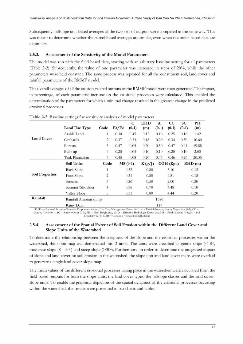
Land cover related parameters that were measured in the field, like plant height (PH), canopy cover (CC)

and surface cover (SC), were built into the Land Use Table that was subsequently associated with the land

cover map in PCRaster. Other secondary parameters that were also built into the table are the ratio of actual

to potential evapotranspiration (Morgan, 2005), crop management factor (C = 1 – CC), rainfall interception

by vegetation (A = Rainy Days * Smax / Annual Rainfall), leaf area index (LAI = ln(1 – CC) / -0.4),

maximum plant canopy storage (“Smax1 = 0.935 + 0.498*LAI - 0.00575 for field crops” or “Smax2 =

1.46*LAI**0.56 for trees”) and effective hydrological depth (Morgan, 2001). Using the lookupscalar

command in PCRaster, individual maps were generated for each parameter based on the land cover map.

2.4.2. Rainfall Data

The cumulative annual rainfall (1,380mm) and number of rainy days (117) were generated from data acquired

from the Royal Meteorology Department of Thailand through the Civil Engineering Department of

Naresuan University, Phitsanulok, Thailand (Appendix 2-5 and Figure 2-16). The lowest rainfall for the

period under review was recorded in March 2018 (3.6mm), while the maximum rainfall was recorded in

August 2018 (301mm).

2.4.3. Topographic Data

The 30m resolution SRTM DEM was resampled to 15m because other model inputs like the land cover

map, had 15m spatial resolution. The resampling consequently ensured that the grid cells of all the model

inputs are well aligned, enabling easy and effective manipulation of model inputs to generate the appropriate

model outputs. Afterwards the slope was computed from the DEM. Finally, the local drainage direction

(LDD) was produced to depict the flow of water from a grid cell to its neighbours, based on the

understanding that water flows in the direction of least resistance, which may also be synonymous with the

direction of steepest slope.

2.5. Erosion Modelling

The runoff and erosion assessment was based on the RMMF erosion modelling methodology reported by

Morgan (2001). The model separates soil erosion into the water phase and the sediment phase. The water

phase determines the erosive energy of rainfall and runoff volume, while the sediment phase determines to

a great extent, the particle detachment by rainfall and runoff, as well as the transport capacity of the runoff.

Figure 2-16: Cumulative monthly rainfall (mm) in Uttaradit, Thailand (2017/2018)

Month Rainfal (mm) Days

Oct-17 133.3 13

Nov-17 5.2 4

Dec-17 25.2 3

Jan-18 7 2

Feb-18 12.3 1

Mar-18 3.6 3

Apr-18 72.7 10

May-18 280.4 18

Jun-18 200.5 15

Jul-18 148 19

Aug-18 301 16

Sep-18 191.1 13

Total 1380.3 117

0

2

4

6

8

10

12

14

16

18

20

0

50

100

150

200

250

300

350

Oct

-17

No

v-1

7

Dec

-17

Jan

-18

Feb

-18

Mar

-18

Ap

r-1

8

May

-18

Jun

-18

Jul-

18

Au

g-1

8

Sep

-18

Rai

ny

Day

s

Rai

nfa

ll (m

m)

Rainfal (mm) Days


15

According to Morgan (2001), particle detachment and runoff transport capacity play a crucial role in the

determination of soil erosion, as the lower of the two variables is representative of the erosion rate.

2.5.1. The RMMF Erosion Modelling Process

1. Rainfall Energy Estimation: Effective rainfall (ER; mm) was considered to be affected by annual

rainfall (R; mm) and the proportion of the rainfall that reaches the ground (A) after some of the rainfall

has been intercepted by plant canopy cover (CC; %). And usually, A is a value that ranges from 0 to 1.

𝐸𝑅 = 𝑅 ∗ 𝐴 … … … … … … … … … … … … … … … … … … … … … … … 𝐸𝑞. 4

Furthermore, Effective Rainfall (ER; mm) is a product of both leaf drainage (LD; mm) and direct Throughfall (DT; mm) of rainfall.

𝐸𝑅 = 𝐿𝐷 + 𝐷𝑇 … … … … … … … … … … … … … … … … … … … … … 𝐸𝑞. 5

The split in the effective rainfall (ER; mm) is a direct function of canopy cover (CC; %)

𝐿𝐷 = 𝐸𝑅 ∗ 𝐶𝐶 … … … … … … … … … … … … … … … … … … . . … … … 𝐸𝑞. 6

𝐷𝑇 = 𝐸𝑅 – 𝐿𝐷 … … … … … … … … … … … … … … … … … … … … … … 𝐸𝑞. 7

The kinetic energy (KE(DT); J/m2) of throughfall is a function of rainfall intensity (I; mm/h)

𝐾𝐸(𝐷𝑇) = 𝐷𝑇(11.9 + 8.7𝑙𝑜𝑔𝐼) … … … … … … … … … … … … … … … 𝐸𝑞. 8

Similarly, kinetic energy of leaf drainage (KE(LD), J/m2) is dependent on plant height (PH; m)

𝐾𝐸(𝐿𝐷) = (15.8 ∗ 𝑃𝐻0.5)– 5.87 … … … … … … … … … … … … … … … 𝐸𝑞. 9

It is noteworthy that if the results of the computation of the kinetic energy of the rainfall is negative, it is assumed to be equal to zero.

2. Estimating Runoff: Runoff (Q; mm) occurs when daily rainfall exceeds soil moisture storage capacity (Rc; mm). It is expressed as:

𝑄 = 𝑅 𝑒−𝑅𝑐𝑅𝑜 … … … … … … … … … … … … … … … … … … … … … … … … 𝐸𝑞. 10

Where Q = Annual Runoff (mm), R = Annual Rainfall (mm), Ro = Mean Rain per Rainy Day (mm), Rc = Soil Moisture Storage Capacity (mm) and Rn = Number of Rainy Days per annum

𝑅𝑜 = 𝑅

𝑅𝑛 … … … … … … … … … … … … … … … … … … … … … … … … 𝐸𝑞. 11

Soil moisture storage capacity (Rc; mm), on its part, was dependent on moisture content at field capacity (MS; %, w/w), bulk density (BD; Mg/m3) and on the ratio of Actual to Potential Evapotranspiration (Et/Eo)

𝑅𝑐 = 1000𝑀𝑆 ∗ 𝐵𝐷 ∗ 𝐸𝐻𝐷(𝐸𝑡 / 𝐸𝑜) … … … … … … … … … … … … 𝐸𝑞. 12

Where Rc = Soil Moisture Storage Capacity (mm), MS = Soil Moisture Content at Field Capacity (%, w/w), BD = Bulk Density (Mg/m3), EHD = Effective Hydrological Depth (m) and Et/Eo = Ratio of Actual to Potential Evapotranspiration

It is noteworthy that according to Morgan (2001) effective hydrologic depth (EHD) indicates the depth

of soil within which the moisture storage capacity controls the generation of runoff. It is a function of

plant cover, which influences rooting depth and root density; and is also sometimes a function of

effective soil depth.

Nevertheless, according to Morgan (2001), all the runoff within a grid are generated in the grid.

Shrestha et al. (2014) was however, of the opinion that the total runoff in a grid is the sum of the runoff

generated within the grid and the runoff flowing into the grid from surrounding grids located on higher

terrain. This is quite logical because runoff is not stagnant, it flows from place to place; the implication

being that it flows from one grid to another as it moves towards the outlet. Shrestha et al. (2014)

incorporated this into the erosion modelling process by using flow accumulation over a gridded

16

landscape to quantify the runoff. The flow direction was first defined in terms of the direction of the

steepest slope, after which, local drainage direction network was generated. The total area contributing

runoff was subsequently calculated for each grid cell.

3. Particle Detachment by Raindrop Impact: Particle detachment by raindrop impact (F; kg/m2) was

a function of soil detachability (K; g/J) and kinetic energy of rainfall (KE)

𝐹 = 𝐾 ∗ 𝐾𝐸 ∗ 10−3 … … … … … … … … … … … … … … … … … … … … 𝐸𝑞. 13

4. Soil Particle Detachment by Runoff: In addition to detachment by raindrop impact (F; kg/m2), soil

particles were also considered to be detachable by runoff (H; kg/m2). Detachment by runoff (H;

kg/m2) is a function of the resistance of the soil (Z), runoff (Q; mm), slope steepness (S; o) and ground

cover (GC; %)

𝐻 = 𝑍𝑄1.5𝑠𝑖𝑛𝑆(1 – 𝐺𝐶) ∗ 10−3 … … … … … … … … … … … … … … … … 𝐸𝑞. 14

However, the underlying assumption is that soil particle detachment occurs when soil protection by

ground cover is not available. Also, the resistance of the soil (Z) was considered to be a function of

soil cohesion (COH; kPa) as measured on saturated soils with a shear vane apparatus.

𝑍 = 1

0.5 ∗ 𝐶𝑂𝐻 … … … … … … … … … … … … … … … … … … … … … … … … 𝐸𝑞. 15

5. Transport Capacity of Runoff: Transport Capacity of Runoff (TC; kg/m2) was a function of Runoff

(Q; mm), Crop or Plant Cover Factor (C) – taken as the product of C and P factors in USLE – and

Slope Angle (S; o)

𝑇𝐶 = 𝐶𝑄2 𝑠𝑖𝑛𝑆 ∗ 10−3 … … … … … … … … … … … … … … … … … … … 𝐸𝑞. 16

6. Estimating Soil Erosion: The summation of the estimated soil particle detachment by runoff and

raindrop impact amounted to the total annual soil detachment. This was then compared with the

annual runoff transport capacity. The lesser of the two values was considered to be equal to the annual

soil erosion rate.

7. Running the RMMF Model: The model was run twice, each time with a different soil data source.

The outputs generated were then assessed statistically to determine the degree of similarity between

the outputs generated from the two data sources. The complete scripts for running the model is shown

in Appendix 2-4.

2.5.2. Comparative Assessment of SoilGrids250m and Field-based Outputs

The difference between the values of the erosional processes generated from SoilGrids250m data and field-

based soil data were calculated. The magnitude of the residual value after one image has been subtracted

from its counterpart is a measure of the similarity of the two sets of output.

Furthermore, 120 random points were generated from the hillslope map using stratified random sampling.

30 points were generated for each hillslope unit. The grid values corresponding to the random points were

then extracted from both sets of model outputs. The average estimate for each hillslope unit was also

calculated. Two sets of comparative assessment were then performed.

First, the two sets of outputs were compared point-by-point, based on the 120 random points. The field-

based output was plotted against the corresponding SoilGrids250m output to determine whether they are

correlated. To determine to what extent the outputs were similar, the Euclidean Distance was calculated. To

determine whether there is a statistically significant difference between the two sets of outputs, T-Test or

Wilkoxon Signed Rank Test was calculated. In both cases, according to Dytham (2011), if the calculated p-

value is less than 0.05, then there is a significant difference between the data sources.


17

Subsequently, hillslope unit-based averages of the two sets of outputs were compared in the same way. This

was meant to determine whether the parcel-based averages are similar, even when the point-based data are

dissimilar.

2.5.3. Assessment of the Sensitivity of the Model Parameters

The model was run with the field-based data, starting with an arbitrary baseline setting for all parameters

(Table 2-2). Subsequently, the value of one parameter was increased in steps of 20%, while the other

parameters were held constant. The same process was repeated for all the constituent soil, land cover and

rainfall parameters of the RMMF model.

The overall averages of all the erosion-related outputs of the RMMF model were then generated. The impact,

in percentage, of each parametric increase on the erosional processes were calculated. This enabled the

determination of the parameters for which a minimal change resulted in the greatest change in the predicted

erosional processes.

Table 2-2: Baseline settings for sensitivity analysis of model parameters

Land Use Type Code Et/Eo

C (0-1)

EHD (m)

A (0-1)

CC (0-1)

SC (0-1)

PH (m)

Arable Land 1 0.30 0.45 0.12 0.16 0.25 0.16 1.42 Land Cover Orchards 2 0.37 0.33 0.18 0.20 0.34 0.50 10.60 Forests 3 0.47 0.05 0.20 0.50 0.47 0.41 19.88 Built-up 4 0.20 0.04 0.10 0.10 0.20 0.10 2.00 Teak Plantation 5 0.45 0.08 0.20 0.47 0.46 0.26 20.35

Soil Units Code MS (0-1) K (g/J) COH (Kpa) EHD (m)

Back Slope 1 0.32 0.80 5.10 0.12 Soil Properties Foot Slope 2 0.31 0.80 4.81 0.18 Streams 3 0.20 0.50 2.00 0.20 Summit/Shoulder 4 0.36 0.70 4.48 0.10 Valley Floor 5 0.31 0.80 4.44 0.20

Rainfall Rainfall Amount (mm) 1380 Rainy Days 117

Et/Eo = Ratio of Actual to Potential Evapotranspiration, C = Crop Management Factor (0-1), A = Rainfall Interception by Vegetation (0-1), CC = Canopy Cover (0-1), SC = Surface Cover (0-1), PH = Plant Height (m), EHD = Effective Hydrologic Depth (m), MS = Field Capacity (0-1), K = Soil

Erodibility (g/J), COH = Cohesion = Shear Strength (Kpa)

2.5.4. Assessment of the Spatial Extent of Soil Erosion within the Different Land Cover and Slope Units of the Watershed

To determine the relationship between the steepness of the slope and the erosional processes within the

watershed, the slope map was demarcated into 3 units. The units were classified as gentle slope (< 8o),

moderate slope (8 – 30o) and steep slope (>30o). Furthermore, in order to determine the integrated impact

of slope and land cover on soil erosion in the watershed, the slope unit and land cover maps were overlaid

to generate a single land cover-slope map.

The mean values of the different erosional processes taking place in the watershed were calculated from the

field-based outputs for both the slope units, the land cover types, the hillslope classes and the land cover-

slope units. To enable the graphical depiction of the spatial dynamics of the erosional processes occurring

within the watershed, the results were presented in bar charts and tables.

18

2.6. Flowchart

The flowchart of methods, outlining the relationships between the adopted methods and the input data is

shown in Figure 2-17.

Figure 2-17: Flowchart of methods


19

3. RESULTS AND DISCUSSION 3.1. Acquisition and Comparative Analysis of Soil Data

The first research question of this study focussed on the determination of the characteristic features of the

soils of the study area. Nevertheless, before this could be done, physiographic map units were generated for

the study area. The range of the SoilGrid250m data values downloaded for the watershed were discussed in

section 3.1.1. In section 3.1.2 the findings from the various hillslope assessments conducted prior to arriving

at the final map units were discussed. Subsequently, the variation in soil properties across the landscape were

discussed in section 3.1.3.

3.1.1. SoilGrids250m Data for the Watershed

The maximum, minimum and mean values of different soil properties from SoilGrids250m across the

hillslope positions of the study area are shown in Table 3-1. While some of data were downloaded directly

from the World Soil Information (ISRIC) directory (gravel, sand, silt, clay, bulk density and organic carbon),

others were generated through the use of Saxton et al. (1986) pedotransfer functions.

Gravel (14 to 43 %), sand (36 to 50 %), silt (24 to 37 %), clay (20 to 32 %), field capacity (26 to 33 %) and

wilting point (13 to 20 %) were relatively uniform across the study area. Mean bulk density was marginally

higher in the valley, but generally ranges from 1.47 to 1.90 Mg/m3. Similarly, soil porosity (46 to 56 %) was

also marginally lower on the valley. The higher bulk density and lower soil porosity may be attributed to the

predominant arable land use of the valleys, which lead to soil compaction. This may also account for the

relatively lower hydraulic conductivity in the valley. Nevertheless, hydraulic conductivity generally ranges

from 9.77 mm/hr to 58.62 mm/hr. Organic matter ranges from 0.9 to 3.20 %, but the mean value was much

lower on the valley. This may also be attributed to the arable land use as Haynes et al. (2003) pointed out

that agricultural activities tend to reduce soil organic matter and microbial biomass.

In tandem with the findings of this study, Herrmann et al. (2007) reported sand, silt, clay, porosity and

organic matter values of 38%, 21%, 41%, 58% and 4.13% respectively for soils of Northern Thailand. Sand,

silt and porosity were within the vicinity of the range of values reported for the SoilGrids250m data. On the

other hand, clay and organic matter were about 28% higher than the maximum values of 32% (clay) and

3.2% (organic matter) reported for SoilGrids250m. The difference may be attributed the fact that the

SoilGrids250m was the product of global soil modelling using machine learning while the data reported by

Herrmann et al. (2007) were generated from the analysis of soil data collected from the field.

Table 3-1: Variability of soil properties from SoilGrids250m across different hillslope positions

SN

Parameter

Summit Back Slope Valley

Min. Max. Mean Min. Max. Mean Min. Max. Mean

1. Gravel (%) 14 43 27 16 43 27 14 43 26

2. Sand (%) 36 50 41 36 50 41 36 50 41

3. Silt (%) 24 37 33 24 37 33 24 37 32

4. Clay (%) 20 32 26 20 31 26 20 32 27

5. Bulk Density (Mg/m3) 1.47 1.90 1.65 1.46 1.90 1.65 1.47 1.90 1.66

6. Soil Porosity (%) 46 56 52 46 56 52 46 56 51

7. Ksat (mm/hr) 10.39 58.62 22.94 9.83 58.62 23.09 9.77 43.37 20.24

8. Field Capacity (%) 26 33 30 26 33 30 26 33 30

9. Wilting Point (%) 13 20 17 13 20 17 13 20 17

10. Organic Matter (%) 0.95 3.20 1.85 0.95 3.20 1.87 0.90 3.20 1.67

20

3.1.2. Generation of Physiographic Map for Representing Soil Variation

Table 3-2 shows the confusion matrix defining the degree of accuracy of field observations of hillslope units

when compared to the hillslopes generated after the field observations were updated with the Google Earth

elevation profile. The accuracy of the field observation, relative to the post-fieldwork assessment, is 65 %.

This seems like a conservative proportion, as the accuracy of on-site assessment was expected to supersede

that of remotely-sensed information. This may, however, not always be the case as the obstruction of view

by tall trees and other structures and the reduced field of view may sometimes becloud the judgement of

the researcher, especially when the terrain is frequently undulating. Furthermore, there is usually no clear

boundary that can be seen in the field to depict the beginning of one class and the end of another. This may

explain why 19 % of the sites were placed in classes just adjacent to the appropriate class, while only the

remaining 17 % were placed further away.

The hillslope unit with the least accuracy was the Shoulder, where 0 % accuracy was recorded. This is in line

with the fact, as noted in the field, that the Shoulder was usually not wide enough to be distinguishable from

the Summit. Consequently, all the field-generated Shoulders were eventually classified as part of the Summit.

On the other hand, the unit with the highest accuracy was the Back Slope. This may also be attributed to

the fact that, as noted in the field, the Back Slope was usually very extensive and easy to distinguish. It

consequently has an accuracy as high as 86%.

Table 3-2: Accuracy assessment of field-generated hillslope units

Post-Fieldwork

Summit Shoulder Back Slope Foot Slope Toe Slope Total Accuracy (%)

Summit 4 2 1 3

10 40

Field Shoulder

3 1 1 5 0

Back Slope

12 2

14 86

Foot Slope

7 2 9 78

Toe Slope

2

8 10 80

Total 4 2 18 13 11 48 65

In order to extrapolate the point-based field data to the entire watershed, the digital delineation of hillslope

positions (Miller & Schaetzl, 2015), the r.geomorphon algorithm in Grass GIS (Jasiewicz & Stepinski, 2013),

the TPI slope and landform algorithm (Deumlich et al., 2010) and the supervised hillslope delineation were

assessed to determine the most adequate for the study.

1. Digital Delineation of Hillslope Positions

Figure 3-1 shows a map of the hillslope as delineated with the method highlighted in Miller & Schaetzl

(2015). It is noteworthy that the dominant landscape position is the Back Slope. This may be the case because

in the course the fieldwork, it was noted that the Back Slope was quite extensive, relative to the other

hillslope positions. However, instead of the 5 hillslope units that should have been delineated, only 3 were

delineated; the Shoulder and the Foot Slope were not delineated. This is in line with the findings during the

fieldwork that the shoulder and the foot slopes are quite narrow, and not easily distinguishable from the

adjacent hillslope positions. Similarly, Miller & Schaetzl (2015) reported that the hillslope positions with the

lowest accuracy were the Shoulder and the Foot Slope. As such, as seen in Table 3-3 much of the Shoulder

and the Foot Slope were delineated as part of the Back Slope. Overall, 100%, 55% and 25% of the Back

Slope, the Toe Slope and the Summit respectively, were delineated accurately. 46% of other hillslope

positions were, however, also delineated as part of the Back Slope.


21

The overall accuracy of the classification delineation was 52%. Irrespective of the fact that none of the

Shoulders and the Foot Slopes were delineated, the accuracy was still comparable to the 62% accuracy

reported by Miller & Schaetzl (2015). Nevertheless, even though the accuracy of the delineation was

relatively high, it was hinged more on the accuracy of Back Slope predictions, which was also grossly

inaccurate because a large proportion of other hillslope positions were wrongly classified as part of the unit.

The poor performance of the delineation may be attributed to the coarse resolution of the DEM used. Miller

& Schaetzl (2015) used a 3m resolution LiDAR DEM, which was able to generate all the 5 hillslope units.

The required detail for running the model was not available in the 30m SRTM DEM that was used in this

study. Resampling the DEM to 3m enabled the running of the model, but it could not generate information

that was not originally present in the parent DEM.

Figure 3-1: Digital hillslope positions

Table 3-3: Accuracy assessment of digital hillslope position delineation

Hillslope Delineation


Summit 1

3

4 25

Field Shoulder

2

2 0

Back Slope

18

18 100

Foot Slope

10

3 13 0

Toe Slope

5

6 11 55

Total 1 0 38 0 9 48 52


22

2. Delineation of Geomorphic Units

Figure 3-2 shows a map of the geomorphic units of the study area, as delineated with the r.geomorphon in

Grass GIS. The map shows that out of the 10 geomorphic units delineated in the study area, the most

prominent were the Slope class – which is also synonymous with the back slope – and the Flats. To make

them comparable to field observations, some of the slope classes were merged due to their similarity, e.g.

Summit, Ridge and Spur; Hollow, Valley and Depression, etc. These may not be perfect matches, but they

were merged to facilitated ease of comparison.

75%, 33% and 100% of the Summit, Back Slope and Toe Slope respectively, were predicted accurately

(Table 3-4). None of the Shoulder and the Foot Slope were correctly predicted. The delineation of the

shoulder as part of the Summit, and the Foot Slope as part of the Toe Slope may be attributed to the fact

that at the 30m resolution of the SRTM DEM, those units are not easy to separate, as was also evident

during the fieldwork. Furthermore, unlike the digital hillslope position algorithm, the r.geomorphon was

apparently unable to predict most of the Back Slope, which had 33% accuracy. This may not necessarily be

the case as some of the Spurs and Hollows / Depressions that were classified as part of the Summit and

Toe Slope respectively, may have been located on the Back Slope.

The overall accuracy was 41.67%. Kramm et al. (2017) reported an accuracy of 39% for 30m SRTM DEM

and 70% for 5m Pléiades Stereo Image, implying that a higher resolution DEM data will yield more

accurately delineated geomorphic units. Irrespective of an accuracy of about 42%, it is still a valuable tool.

Moreover, the generated geomorphic units were quite distinct from the five hillslope positions to which

they were compared. If these units were delineated prior to the fieldwork, soil samples may have been

collected from each of the delineated units, and the accuracy may have been much higher.

Figure 3-2: Geomorphic units



23

Table 3-4: Accuracy assessment of geomorphic units

Geomorphic Units


Summit 3

1 4 75

Field Shoulder 2

2 0

Back Slope 4

6

8 18 33

Foot Slope 4

2

7 13 0

Toe Slope

11 11 100

Total 13 0 8 0 27 48 41.67

3. Delineation of TPI Slope Units

Figure 3-3 shows a map of the TPI slope units. The map indicates that the dominant hillslope units are

Summit/Top/Ridge and the Depressions. Expectedly, as shown in Table 3-5, the Summit and the Toe Slope

were over-predicted, as other hillslope units were delineated as part of both units. The overall accuracy of

the delineated hillslope units was 35%. Kramm et al. (2017) reported an accuracy of 41%. The higher

accuracy may be attributed to the fact that they compared the delineated classes with field assessment of the

same nomenclature. This result shows that the TPI slope algorithm was mainly able to separate lowland

from upland areas. This is in line with the assertion of Weiss (2001) that the classification enables the

delineation of mountains, ridgelines and valleys.

Figure 3-3: TPI slope units


24

Table 3-5: Accuracy assessment of TPI slope units

TPI Slope Units


Summit 4

4 100

Field Shoulder 2

2 0

Back Slope 5

1 3 9 18 6

Foot Slope

1 1 1 10 13 8

Toe Slope

11 11 100

Total 11 1 2 4 30 48 35

4. Delineation of TPI Landform Units

Figure 3-4 shows a map delineating the watershed into its constituent TPI Landforms. It shows that the

landscape was delineated into 10 landform units. Nevertheless, at first glance, with respect to delineating the

hillslope according to field observations, the map units seemed meaningless because virtually the entire area

was classified into small depressions, larger depressions and culmination area. Small and large depressions

may be correlated to Toe Slope, while culmination area does not seem to belong to any of the hillslope units

(Table 3-6). By implication, 88% of the sample sites were classified as Toe Slope (small depressions, larger

depressions, hollows and flats), while 10.42% was classified as Culmination Area, giving an overall accuracy

of 25.58%. However, on closer observation, it was realized that 75% of the Summit and 50% of the Shoulder

were classified as Culmination Area. It consequently became apparent that the landform units may be very

useful in separating the Summit and Shoulder from other landscape units. Nevertheless, the Culmination

Area seemed to be more extensive than the Summit/Shoulder should have been; besides, no site was

delineated as Top / Shoulder or Local Elevation in Lowlands.

To explore the possibilities further, the SRTM DEM was resampled from 30m to 5m, to reflect the 5m

resolution of the airborne laser-derived 5m DEM used by Deumlich et al. (2010) in the course of assessing

the functionality of the algorithm. This finer resolution was able to separate the Top/Shoulder class from

the Culmination Area, as the 75% of the Summit that was classified as Culmination Area became classified

as a Top/Shoulder surrounded by the Culmination Area (Table 3-7). As such, even though the algorithm

was still only able to separate the landscape into upland (culmination area) and lowland areas, it was able to

isolate the summit within the culmination area. In addition to that, some Summit and Shoulders were still

delineated as part of the Culmination Area.

The ability of the model to isolate the Top/Shoulder from the Culmination Area may be attributed to the

interaction of the of the pixel values of the grid cells and the neighbourhood defined by the circle of arbitrary

radius. Figure 3-5 shows a schematic DEM with 30m grid cells. These grid cells were subsequently resampled

to 5 by 6m grid cells. Given an arbitrary radius of 25m, when the pixel value of the central 30m grid was

compared to the average pixel value of the neighbourhood defined by the 25m radius, only one coarse value

was generated for the entire grid. On the other hand, when the pixel value of each of the numbered 5 by

6m grid cells is compared with the average pixel values of the same neighbourhood size, the same calculation

is repeated 30 times. Based on the impact of the neighbourhood average on each of these fine grid cells, it

was able to isolate terrains that the larger grid cells could not isolate. This is in tandem with the assertion of

Weiss (2001) and Jenness (2006) that topographic position index is scale-dependent.


25

Figure 3-4: TPI landform units

Table 3-6: Accuracy assessment of TPI landform units using a 30m DEM

TPI Landform (30m DEM)

Summit Shoulder Back Slope Foot Slope Toe Slope Total Accuracy (%) Cul. Area

Summit

1 1 0 3

Field Shoulder

1 1 0 1

Back Slope

1

17 18 5.56 1

Foot Slope

13 13 0

Toe Slope

10 10 100

Total 0 0 1 0 42 43 25.58 5

Table 3-7: Accuracy assessment of TPI landform units using a 5m DEM

TPI Landform @ 5m

Summit Shoulder Back Slope Foot Slope Toe Slope Total Accuracy (%) Cul. Area

Summit 3

3 100 1

Shoulder

1 1 0 1

Field Back Slope 2

14 16 0 1

Foot Slope

13 13 0

Toe Slope

11 11 100 1

Total 5 0 0 0 39 44 31.818


26

Figure 3-5: Grid cells showing the interactive effects of cell size and arbitrary radius on the generation of

the TPI landform

5. Supervised Hillslope Delineation

Flow accumulation (Figure 3-6a), elevation (Figure 3-6b), profile curvature (Figure 3-6c) and slope (Figure

3-6d) data were generated for each of the sample sites. The data was explored to get an overview of their

respective ranges for each hillslope position. Figure 3-6a shows that flow accumulation was generally low

for the study area, except for the Toe Slope where it was relatively high, with an outlier as high as 449. The

unit originally had outliers as high as 4,548, which were deleted and classified as part of the stream beds.

Nevertheless, the Toe Slope still had the highest flow accumulation, ranging from 3.5 to 449. This may be

attributed the fact that Toe Slopes are ideally the lowest points on the landscape, relative to other hillslope

positions. As such, all the runoff generated in the higher altitudes end up in the Toe Slope. As a consequence,

cells with very high flow accumulation are either on the Toe Slope or on the stream beds.

Generally, elevation was least on the Toe Slope, with a median value of 169m, even though the lowest

elevation was recorded on the Foot Slope (112m) (Figure 3-6b). This was an expected outcome because the

Toe Slopes and the Foot Slopes are adjacent and are located at the bottom of the landscape. The range of

elevations did not however seem to show a specific pattern related to hillslope. For instance, the summits,

just like other position, can be found on higher as well as lower terrains. More so, the site with the highest

elevation was located on the back slope. This was attributed to the heterogeneity of the landscape. If the

study area had been located on a single hillslope, then we would have had a sequence of elevations that align

with the different positions of the landscape. This was, however, not the case, as we had numerous high and

low hillslopes within study area. The median values were, however, higher for the summit and shoulder,

decreasing afterwards from the Back Slope through the Foot Slope to the Toe Slope. This is in line with the

findings of Miller & Schaetzl (2015), who reported high relative elevation for Summit and Shoulder, medium

elevation for Back Slope and low elevation for Foot Slope and Toe Slope.

The Back Slope has the widest range of curvature values, ranging from -1.244 to 1.380 (Figure 3-6c). This

implies that the Back Slope has regions that are concave (positive), regions that are convex (negative) and

regions that are even (zero). The shoulder and the Summit generally had negative values, implying that they

are convex. The Foot Slope and Toe Slope were mostly positive (concave), with median values close to zero

(even). On the other hand, Miller & Schaetzl (2015), reported linear profile curvature for Summit, Back

Slope and Toe Slope, concave curvature for the Foot Slope and convex curvature for the Shoulder. With

regards to the curvature of the Shoulder and the Foot Slope, both studies were in agreement. The marginal

disagreement with respect to other hillslope positions may be attributed to the heterogeneity of the Ban Dan

Na Kham watershed.


27

The Back Slope had the steepest slope (27o) and the widest range of slope values (5 – 27o) (Figure 3-6d). On

the other hand, the Shoulder has the least median slope values (4o), though the Summit and the Toe Slope

values were also low. This was also in line with the findings of Miller & Schaetzl (2015) , who reported that

the Back Slope had high slopes, the Summit and Toe Slope had low slopes, while the Shoulder and Foot

Slope had medium slopes. The fact that the Shoulder of the study area had relatively low slopes may be

attributed to the peculiarities of the terrain as noted during the fieldwork, with particular reference to the

relative narrowness of the Shoulder, which made it difficult to separate it from the Summit.

These values were used to generate the decision rules (Table 2-1) which enabled the classification of the

Supervised Hillslopes in ArcMap using the vector file generated in eCognition through the segmentation of

slope, profile curvature, flow accumulation and elevation raster maps. The constituent units of the generated

map are the Back Slope, Foot Slope, High Stream Beds, Low Stream Beds, Shoulder, Streams, Summit and

Toe Slope. It is however noteworthy that none of the sampled Shoulder or Summit sites were correctly

delineated (Table 3-8). While 50% of the Back Slope, 54% of the Foot Slope and 55% of the Toe Slope

were correctly delineated, the overall accuracy was 46%. Furthermore, 38% of the units were placed in

positions just adjacent to the appropriate unit, while only about 16% were delineated in units farther away

from the appropriate one. The relatively low performance may be attributed to the heterogeneity of the

terrain. The placement of 38% in units just adjacent to the appropriate ones is also an indication the model

efficiency may be improved greatly with minor adjustments. Collectively, it consequently performed better

that the other hillslope classifications with regards to the delineation of the Back Slope, the Foot Slope and

the Toe Slope. With regards to the overall accuracy, it had lower accuracy than the digital hillslope position

Figure 3-6: Variation in flow accumulation (a), elevation (b), profile curvature (c) and slope (d) across the sample sites

28

delineation, which had an accuracy of 52%. It was, however, more robust, as it did not concentrate most of

the sampled sites in one hillslope unit.

Table 3-8: Accuracy assessment of supervised hillslope delineation

Supervised Hillslope


Summit

2 2

4 0

Field Shoulder

1 1

2 0

Back Slope

1 9 8

18 50

Foot Slope

5 7 1 13 54

Toe Slope

3 2 6 11 55

Total 0 1 19 20 6 48 46

6. Final Hillslope Units

None of the implemented hillslope classification systems was able to effectively delineate all hillslope units.

Some, like the TPI Landform were good for the delineation of the summit / shoulder, the upland areas

(culmination area) and the lowland areas, while others, like the supervised classification system, were better

for the delineation of the back slope, the foot slope and the toe slope. Consequently, to arrive at the final

soil units, these two methods were combined.

Figure 3-7 shows a map generated from the combination of the Supervised Hillslope and the TPI Landform

Classes. The Top / Shoulder of the TPI landforms was adopted, while all other units of the Supervised

Hillslope were retained. Furthermore, the Low Stream Beds were merged with the Streams, while the High

Stream Beds were merged with the Toe Slope. The final map has five units, viz. Back Slope, Foot Slope,

Streams, Summit/Shoulder and Valley Floor.

Figure 3-7: Geomorphic map units for characterizing soil variation across the watershed



29

3.1.3. Assessment of the Soil Variation Across the Landscape

The field-generated soil data are presented in tables and graphs in this section. Appendix 3-1 shows the

morphologic properties of the sample sites while Appendix 3-2 shows the physicochemical properties.

Figure 3-8a to Figure 3-8f and Figure 3-9a to Figure 3-9d depict the minimum, median, maximum, range

and mean of different physicochemical soil properties in the different hillslope positions of the study area.

Figure 3-10a to Figure 3-10f and Figure 3-11a to Figure 3-11d depict the minimum, median, maximum,

range and mean of the different physicochemical properties of the soils underlying the sampled land cover

types in the study area.

A. Variability of Soil Physicochemical Properties Across the Hillslope Positions

A wide range of variability of sand content was recorded on all the hillslope positions (Figure 3-8a). Except

for the Summit/Shoulder, which had the lowest mean (29%) and median values (22%), all the other hillslope

positions had similar mean sand content, ranging from 34 to 36%. The lower sand content on the

Summit/Shoulder may be attributed to the relatively lower flow accumulation (Figure 3-6a) and slope

(Figure 3-6d), which ensured that the less of the finer materials (clay and silt), were eroded and lost. This is

in line with the findings of Oku et al. (2010), who reported lower sand content for the Summit of humid

tropical forest soils. Overall, the value was similar to the 38% sand content reported by Herrmann et al.

(2007) for the soils of Northern Thailand.

Similarly, the mean silt content for the Back Slope, the Foot Slope and the Valley Floor were similar, ranging

from 41 to 43%, and lowest on the Summit/Shoulder (38%) (Figure 3-8b). Silt was however higher than the

31 % silt content reported by Herrmann et al. (2007) for the soils of Northern Thailand. This may be

attributed to a possible difference in the underlying geologic formations of the two study areas.

Clay content was distinctly higher on the Summit/Shoulder (33%), and least in the Foot Slope (20%) (Figure

3-8c). This is also in line with the findings of Oku et al. (2010) for humid tropical forest soils. This may be

attributed to the relatively lower flow accumulation (Figure 3-6a) and slope (Figure 3-6d) in the

Summit/Shoulder, coupled with the fact that clay tends to stick together and has relatively greater resistance

to detachment than the other particle size fractions.

Bulk density was least on the Summit/Shoulder (1.08 Mg/m3), progressively increasing from the

Summit/Shoulder to the Valley Floor (1.31 Mg/m3), where it was highest (Figure 3-8d). This may be

attributed to the impact of different land use types, as much of the Summit/Shoulder are either natural

forest or plantations. The reduced human activities result in reduced compaction, which in turns, results in

reduced bulk density. On the other hand, the valley floor, which had the highest bulk density of 1.31 Mg/m3,

was dedicated almost exclusively to arable crops. These agricultural and other anthropogenic activities result

in increased soil bulk density. This is in line with the contention of Kodiwo et al. (2014) that increased

intensity of agricultural activities results in increased soil compaction, which in turns results in increased

bulk density.

Conversely, soil porosity was highest on the Summit/Shoulder (59%), and least on the Valley Floor (51%)

(Figure 3-9a). Naturally, it may have been expected that since the Summit/Shoulder had more clay, it should

be less porous than the other hillslope positions with lower clay. However, the effect of human activities on

bulk density also translates into the reduced porosity of the arable soils on the Valley Floor. This is in line

with the contention of Balan et al. (2009) that a negative correlation exists between bulk density and soil

porosity. Similarly, Pagliai & Vignozzi (2006) reported that soil porosity decreases with increase in soil

compaction.

The widest range of shear strength was recorded on the Summit/Shoulder (2.43 to 6.05 kPa), which also,

incidentally, had the lowest median values of 4.70 kPa (Figure 3-9b). The average shear strength was least

30

on the Summit/Shoulder (4.48 kPa) and the Valley Floor (4.44 kPa), while the highest mean value was

recorded on the Back Slope (5.09 kPa). The low shear strength of the Valley Floor may be attributed to the

effect of tillage activities in the agricultural fields, which break up the soil structure, reducing their resistance

to rupture. On the other hand, the lower shear strength of the Summit/Shoulder may be attributed to the

effects of large trees roots moving through the soil and the activities of a diverse range of soil macro fauna.

In line with this, Whitford & Eldridge (2013) contended that the activities of termites, like many other

macrofauna, affect the bulk density, porosity, aeration, infiltration, water holding capacity, turnover and

homogenization dynamics of tropical soils. This complex interaction may account for the reduced

compaction and shear strength of forest soils.

The soil unit with the highest range and extent of saturated hydraulic conductivity (12.15 to 98.43 mm/hr)

was located on the Foot Slope (Figure 3-9c). The least mean saturated hydraulic conductivity of 11.15

mm/hr was recorded on the Summit/Shoulder, which incidentally, also has the highest clay content (Figure

3-8c). The fact that saturated hydraulic conductivity of the Summit/Shoulder was distinctly different may

be attributed to the fact that its texture was also distinctly different (Figure 3-8a, b, c). This is in line with

the findings of Sarki et al. (2014) that, relative to other textural classes, soils with high clay content have very

low saturated hydraulic conductivity.

Moisture content at field capacity (Figure 3-9e) and wilting point (Figure 3-9f) were higher on the

Summit/Shoulder (35% and 21% respectively), generally decreasing down the slope. This is also attributable

to the soil texture, as clayey tends to have higher moisture holding capacity than sandy soils. It may

consequently be concluded that the Summit/Shoulder had higher moisture content at field capacity and

(a)

Mean: 29.25 34.44 36.06 35.75

Mean: 37.50 41.67 43.61 42.13

Mean: 33.25 24.00 20.39 22.00

Mean: 1.08 1.12 1.28 1.31

Figure 3-8: Spatial variability of sand (a), silt (b), clay (c) and bulk density (d) across the study area

(b)

(c) (d)


31

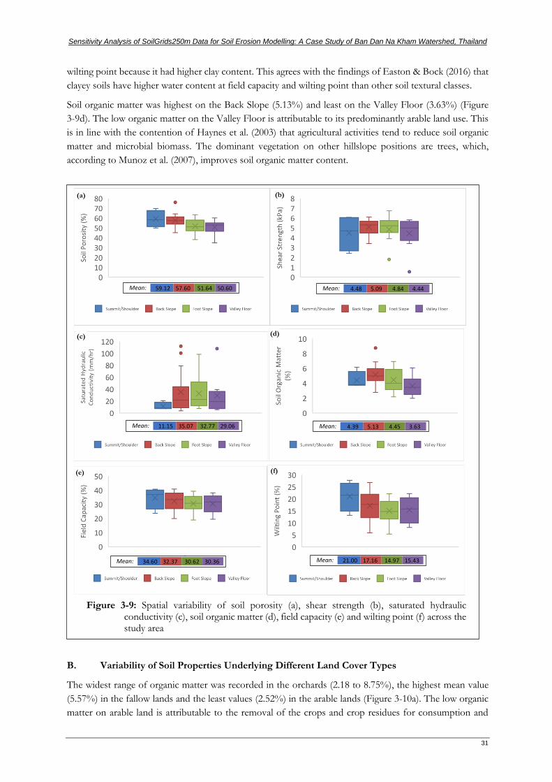
wilting point because it had higher clay content. This agrees with the findings of Easton & Bock (2016) that

clayey soils have higher water content at field capacity and wilting point than other soil textural classes.

Soil organic matter was highest on the Back Slope (5.13%) and least on the Valley Floor (3.63%) (Figure

3-9d). The low organic matter on the Valley Floor is attributable to its predominantly arable land use. This

is in line with the contention of Haynes et al. (2003) that agricultural activities tend to reduce soil organic

matter and microbial biomass. The dominant vegetation on other hillslope positions are trees, which,

according to Munoz et al. (2007), improves soil organic matter content.

B. Variability of Soil Properties Underlying Different Land Cover Types

The widest range of organic matter was recorded in the orchards (2.18 to 8.75%), the highest mean value

(5.57%) in the fallow lands and the least values (2.52%) in the arable lands (Figure 3-10a). The low organic

matter on arable land is attributable to the removal of the crops and crop residues for consumption and

(a)

Mean: 59.12 57.60 51.64 50.60

Mean: 4.48 5.09 4.84 4.44

Mean: 11.15 35.07 32.77 29.06

Mean: 4.39 5.13 4.45 3.63

Mean: 34.60 32.37 30.62 30.36

Mean: 21.00 17.16 14.97 15.43

Figure 3-9: Spatial variability of soil porosity (a), shear strength (b), saturated hydraulic conductivity (c), soil organic matter (d), field capacity (e) and wilting point (f) across the study area

(b)

(c) (d)

(e) (f)

32

industrial purposes. This is in direct contrast to forests, plantations, orchards and fallow lands where the

plants remain in the field for prolonged periods of time; and even when they die or drop their leaves, these

plant remains decay on the same land and get converted into soil organic matter. As such, Haynes et al.

(2003) asserted that agricultural activities reduce soil organic matter and microbial biomass.

Sand content had the highest range of variability (9.58 to 55.4%) in the long kong orchards (Figure 3-10b).

The mean values were, however, highest in the teak plantations (52%) and lowest in the forests (25%). Silt

content was least on arable lands (35%) and highest in the long kong orchards (45%) (Figure 3-10c). Clay

content was most variable in the long kong orchard (5 to 45%), least mean value was recorded in teak

plantations (8%) and highest in forested lands (32%) (Figure 3-10d). Nevertheless, the land use does not

play a prominent role in determining the soil texture. On the contrary, the soil texture determines the land

use type adopted. Lowland rice fields, for instance, would not be located on sandy soils if clayey soils are

available in adequate amount. Nonetheless, on the long run, the land use may come to affect the soil texture

as certain land uses, like arable land use on steep slopes, may predispose the soil to erosion, and the eventual

loss of much of the silt content of such soils.

Bulk density was highest on arable lands (1.54 Mg/m3) and least on forested (1.08 Mg/m3) and fallow lands

(1.07 Mg/m3) (Figure 3-10e). This is due to human activities or its absence. As Haynes et al. (2003) pointed

out, agricultural activities tend to reduce soil organic matter and microbial biomass. The activities of soil

micro and macro fauna, including the pores they create when they bore through the soil and the

consumption and defecation of soil and organic materials increases soil porosity, which in turns reduces

bulk density. Similarly, the continued addition of organic matter to the soil also reduces soil bulk density

(Sakİn, 2012). These factors account for the lower bulk density on forested and fallow lands and the

increased bulk density on arable lands. Furthermore, Hakansson (2005) asserted that increased use of

agricultural machineries results in increased soil compaction, which in turns, results in increased bulk density.

Shear strength was lowest on arable lands (2.26 kPa) and highest in long kong orchards (5.22 kPa) (Figure

3-10f). This is also attributable to the impact of tillage activity on soil structure. Tillage tends to break up

the soil structure, consequently decreasing their resistance to rupture, which in turns leads to decreased shear

strength. On the other hand, the soils of the long kong orchards had higher shear strength because in

addition to not being tilled, the persistent movement of humans through the orchard results in increased

compaction and greater shear strength. Similarly, Genet et al. (2008) asserted that trees increase shear

strength through their root system, but Genet et al. (2006), contended that due to their higher root area

ratio, the impacts of young trees is greater than that of older trees. This was reiterated by Genet et al. (2008),

Genet et al. (2010) and Fattet et al. (2011), who contended that root biomass density was lower in old natural

forests, which may account for relatively lower impacts on increased shear strength. This may explain why

the soils of long kong orchards, which are relatively younger trees than natural forests and teak plantations,

had higher shear strength.

Soil porosity was highest on fallow lands (60%) and forests (59%) and least on arable lands (42%) (Figure

3-11a). This may be attributed to increased organic matter and activities of soil flora and fauna in the forested

and fallow lands. Saturated hydraulic conductivity was most variable on teak plantations (26.20 to 112.08

mm/hr) and fallow lands (26.38 to 103.55 mm/hr) (Figure 3-11d). The mean value was lowest on forested

soils (12.23 mm/hr) and arable lands (16.42 mm/hr). The low saturated hydraulic conductivity on forested

soils may be attributed to its predominantly clayey texture, while that of arable lands may be attributed to

soil compaction by tillage operations, machineries and other anthropogenic activities. The highest average

saturated hydraulic conductivity of 84 mm/hr was recorded in the soils underlying the teak plantations. This

high conductivity may be attributed to its very low clay content of 8% (Figure 3-11d).


33

Moisture content at field capacity (Figure 3-11b) and wilting point (Figure 3-11c) were highest on forested

lands (36% and 21% respectively) and least on teak plantations (22% and 8% respectively). The higher field

capacity and wilting point in the forest soils may be attributed to its high clay content of up to 32% (Figure

3-11d). Furthermore, the constituent flora and fauna and the organic matter generated also play a crucial

role. Bhadha et al. (2017) reported that increased soil organic matter results in increased soil water holding

capacity. The forests have a dense undergrowth of grasses, shrubs, ferns and herbs, all of which support a

diverse variety of soil fauna, resulting in increased soil organic matter. On the other hand, the teak

plantations were usually almost bare, with relatively few dead leaves to be decomposed and converted into

organic matter. Consequently, the organic matter dynamics in both soils account for some of the variation

in soil water content at field capacity and wilting point.

Mean: 2.52 5.57 4.08 4.86 4.48 4.68

Mean: 40 50 44 29 52 25

Mean: 35 43 43 45 43 39

Mean: 27 10 17 27 8 32

Mean: 1.54 1.07 1.40 1.15 1.25 1.08

Mean: 2.26 5.07 4.73 5.22 5.07 4.60

Figure 3-10: Spatial variability of organic matter (a), sand (b), silt (c), clay (d), bulk density (e) and shear strength (f) in the soils underlying the various land cover types of the study area

(a) (b)

(c) (d)

(e) (f)

34

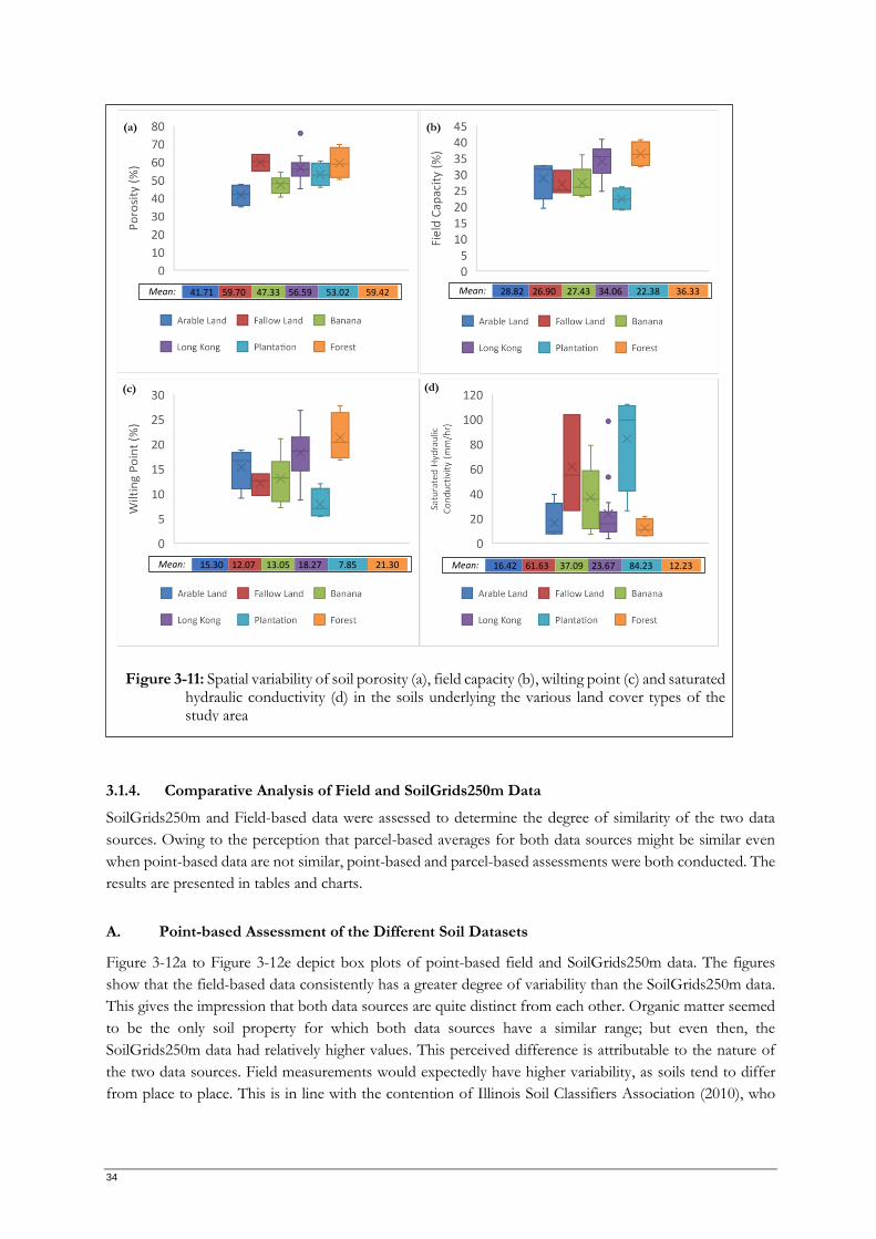
3.1.4. Comparative Analysis of Field and SoilGrids250m Data

SoilGrids250m and Field-based data were assessed to determine the degree of similarity of the two data

sources. Owing to the perception that parcel-based averages for both data sources might be similar even

when point-based data are not similar, point-based and parcel-based assessments were both conducted. The

results are presented in tables and charts.

A. Point-based Assessment of the Different Soil Datasets

Figure 3-12a to Figure 3-12e depict box plots of point-based field and SoilGrids250m data. The figures

show that the field-based data consistently has a greater degree of variability than the SoilGrids250m data.

This gives the impression that both data sources are quite distinct from each other. Organic matter seemed

to be the only soil property for which both data sources have a similar range; but even then, the

SoilGrids250m data had relatively higher values. This perceived difference is attributable to the nature of

the two data sources. Field measurements would expectedly have higher variability, as soils tend to differ

from place to place. This is in line with the contention of Illinois Soil Classifiers Association (2010), who

Figure 3-11: Spatial variability of soil porosity (a), field capacity (b), wilting point (c) and saturated hydraulic conductivity (d) in the soils underlying the various land cover types of the study area

Mean: 41.71 59.70 47.33 56.59 53.02 59.42

Mean: 28.82 26.90 27.43 34.06 22.38 36.33

Mean: 15.30 12.07 13.05 18.27 7.85 21.30

Mean: 16.42 61.63 37.09 23.67 84.23 12.23

(a) (b)

(c) (d)


35

asserted that soils can vary greatly within a very short distance. On the other hand, models are a

simplification of reality; and simplicity comes at a cost.

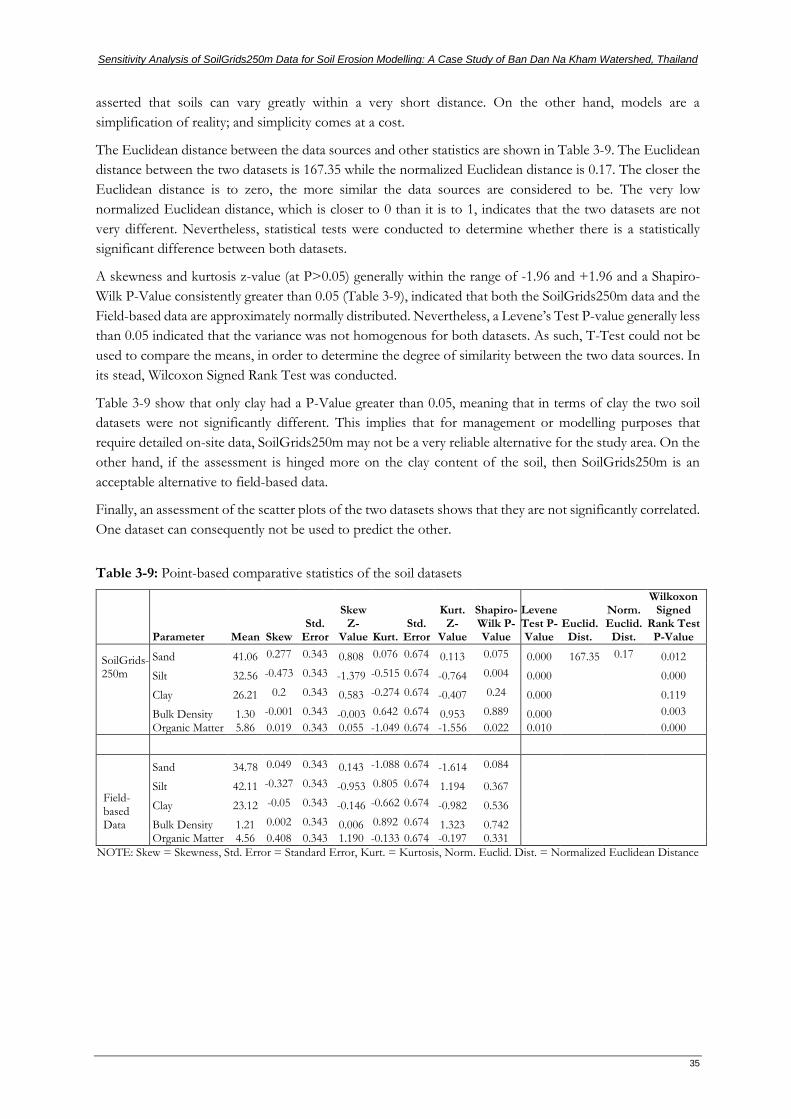
The Euclidean distance between the data sources and other statistics are shown in Table 3-9. The Euclidean

distance between the two datasets is 167.35 while the normalized Euclidean distance is 0.17. The closer the

Euclidean distance is to zero, the more similar the data sources are considered to be. The very low

normalized Euclidean distance, which is closer to 0 than it is to 1, indicates that the two datasets are not

very different. Nevertheless, statistical tests were conducted to determine whether there is a statistically

significant difference between both datasets.

A skewness and kurtosis z-value (at P>0.05) generally within the range of -1.96 and +1.96 and a Shapiro-

Wilk P-Value consistently greater than 0.05 (Table 3-9), indicated that both the SoilGrids250m data and the

Field-based data are approximately normally distributed. Nevertheless, a Levene’s Test P-value generally less

than 0.05 indicated that the variance was not homogenous for both datasets. As such, T-Test could not be

used to compare the means, in order to determine the degree of similarity between the two data sources. In

its stead, Wilcoxon Signed Rank Test was conducted.

Table 3-9 show that only clay had a P-Value greater than 0.05, meaning that in terms of clay the two soil

datasets were not significantly different. This implies that for management or modelling purposes that

require detailed on-site data, SoilGrids250m may not be a very reliable alternative for the study area. On the

other hand, if the assessment is hinged more on the clay content of the soil, then SoilGrids250m is an

acceptable alternative to field-based data.

Finally, an assessment of the scatter plots of the two datasets shows that they are not significantly correlated.

One dataset can consequently not be used to predict the other.

Table 3-9: Point-based comparative statistics of the soil datasets

Parameter Mean Skew Std.

Error

Skew Z-

Value Kurt. Std.

Error

Kurt. Z-

Value

Shapiro-Wilk P-Value

Levene Test P-Value

Euclid. Dist.

Norm. Euclid.

Dist.

Wilkoxon Signed

Rank Test P-Value

SoilGrids-250m

Sand 41.06 0.277 0.343 0.808 0.076 0.674 0.113 0.075 0.000 167.35 0.17 0.012

Silt 32.56 -0.473 0.343 -1.379 -0.515 0.674 -0.764 0.004 0.000 0.000

Clay 26.21 0.2 0.343 0.583 -0.274 0.674 -0.407 0.24 0.000 0.119

Bulk Density 1.30 -0.001 0.343 -0.003 0.642 0.674 0.953 0.889 0.000 0.003

Organic Matter 5.86 0.019 0.343 0.055 -1.049 0.674 -1.556 0.022 0.010 0.000

Field-based Data

Sand 34.78 0.049 0.343 0.143 -1.088 0.674 -1.614 0.084

Silt 42.11 -0.327 0.343 -0.953 0.805 0.674 1.194 0.367

Clay 23.12 -0.05 0.343 -0.146 -0.662 0.674 -0.982 0.536

Bulk Density 1.21 0.002 0.343 0.006 0.892 0.674 1.323 0.742 Organic Matter 4.56 0.408 0.343 1.190 -0.133 0.674 -0.197 0.331

NOTE: Skew = Skewness, Std. Error = Standard Error, Kurt. = Kurtosis, Norm. Euclid. Dist. = Normalized Euclidean Distance

36

B. Parcel-based Assessment of the Different Soil Datasets

Figure 3-13a to Figure 3-13e depicts box plots of parcel-based field and SoilGrids250m data. The average

soil unit data were compared with the average SoilGrid250m data that corresponds to the same area. The

results show that the field-based data still consistently had a greater degree of variability. Also, the

SoilGrids250m data tended to have higher values, with the exception of silt content, which was somewhat

higher for the field-based data (Figure 3-13b).

Figure 3-12: Comparative point-based assessment of sand (a), silt (b), clay (c), bulk density (d)

and organic matter (e) from field-based and SoilGrids250m data

(a) (b)

(c) (d)

(e)


37

The Euclidean distance between the data sources and other statistics are shown in Table 3-10. The Euclidean

distance between the two datasets was 26.25 while the normalized Euclidean distance was 0.19. Even though

the Euclidean distance is much lower that the value (167.35) recorded during the point-based assessment,

the normalized Euclidean distance was still very close to the value (0.17) reported for point-based

assessment. This may be attributed to the fact that irrespective of the fact that the number of values being

compared are different, the datasets are still the same. The very low normalized Euclidean distance,

corroborates the results from the point-based assessment, indicating that the datasets may be similar.

To determine whether the difference was statistically significant, a test of normality and homogeneity of

variance was first conducted to determine which statistical method was appropriate for the available data.

The skewness z-value and the kurtosis z-value (between -1.96 and +1.96) and Shapiro-Wilk P-value (> 0.05),

all indicate that both datasets are approximately normal. The Levene Test results show that only silt and

organic matter had approximately homogenous variance at P>0.05, but at P>0.01, all of them, with the

exception of bulk density, recorded approximate homogeneity of variance. Because the number of parcels

(hillslope units) were equal to 4, which is less than the minimum of 6 samples recommended by Dytham

(2011) as a pre-condition for performing the Wilcoxon Signed Rank Test, the T-Test was calculated at 0.01

level of significance.

T-Test P-values of 0.624 and 0.189, for clay and bulk density respectively, indicate that these parameters

were not significantly different for both data sources at P>0.05. Similarly, a P-value of between 0.011 and

0.019 indicate that sand and organic matter are not significantly different for both data sources at P>0.01.

Silt, with a P-value of 0.008, was however, significantly different at both levels of significance.

This implies that, though the SoilGrids250m and the field-based data were significantly different when

compared point by point, they are quite similar when the average values of an area are compared.

Consequently, when detailed on-site data are not required to effectively implement a project or inform a

decision-making process, SoilGrids250m is a good alternative to field-based soil data. In such a situation,

the use of SoilGrids250m data will save a lot of time, money and energy.

Table 3-10: Parcel-based comparative statistics of the soil datasets


Error

Skew Z-

Value Kurt. Std.

Error

Kurt. Z-

Value

Shapiro-Wilk P-Value

Levene Test P-

Value Euclid.

Dist.

Norm. Euclid.

Dist.

T-Test P-

Value

SoilGrids

-250m

Sand 41.02 -1.298 1.014 -1.28 1.098 2.619 0.419 0.338 0.032 26.25 0.19 0.019

Silt 32.46 -0.106 1.014 -0.11 1.277 2.619 0.488 0.887 0.072 0.008

Clay 26.52 1.119 1.014 1.10 0.927 2.619 0.354 0.076 0.036 0.624

Bulk Density 1.29 0.383 1.014 0.38 -2.918 2.619 -1.114 0.624 0.000 0.189

Organic Matter 6.10 -1.095 1.014 -1.08 -0.036 2.619 -0.014 0.296 0.736 0.011

Field-

based

Data

Sand 33.82 -1.952 1.014 -1.93 3.853 2.619 1.471 0.016

Silt 41.23 -1.09 1.014 -1.08 1.941 2.619 0.741 0.601

Clay 24.95 1.827 1.014 1.80 3.438 2.619 1.313 0.594

Bulk Density 1.20 -0.093 1.014 -0.09 -5.206 2.619 -1.988 0.226 Organic Matter 4.39 -0.193 1.014 -0.19 1.491 2.619 0.569 0.759

NOTE: Skew = Skewness, Std. Error = Standard Error, Kurt. = Kurtosis, Norm. Euclid. Dist. = Normalized Euclidean Distance

38

3.2. Land Use / Land Cover Map

The land use map of the watershed is shown in Figure 3-14. The dominant land uses in the area are arable

farming, orchards – mostly long kong orchard – teak plantations, natural forests and built-up areas. The

accuracy assessment report and confusion matrix for the land use classification is shown in Table 3-11. The

overall accuracy of the land use map is 68%. Natural Forest had a low accuracy of 43% and was mostly

misclassified as Teak Forest or Orchards. This is similar to the findings of Gebhardt et al. (2015), who

reported an accuracy of 50% for secondary forest because it was usually confused with primary forests.

These can be attributed to the fact that all the afore-mentioned land cover types are populated by trees. The

similarity of the two land cover classes is evident in Table 3-13. The canopy cover (92 – 95 %), the plant

Figure 3-13: Comparative parcel-based assessment of sand (a), silt (b), clay (c), bulk density (d) and organic matter (e) from field-based and SoilGrids250m data

(a) (b)

(c) (d)

(e)


39

height (19 – 20m), leaf area index (6 – 7 m2/m2)) and the Et/Eo (0.90 – 0.95), all had similar values. They

may consequently have similar pixel values.

Furthermore, the relatively low producer accuracy recorded for built-up areas (53%) may be attributed to

the misclassification of built-up areas as arable land. Ideally, it is expected that arable land and built-up areas

would have very distinct pixel values. Nevertheless, the watershed is located in a rural setting where a

building might be surrounded by farms, orchards or trees. As such, the building may be located in a pixel

dominated by arable land, resulting in its classification as an arable land. However, with respect to erosion

assessment for the watershed, most of the arable lands and built-up areas are located in relatively flat, low-

lying areas that are less prone to erosion. The misclassification may consequently not have a major effect on

the model-generated erosion prediction.

Forest, arable land and teak had the lowest kappa coefficient of 0.40, 0.53 and 0.56 respectively, whereas,

Built-up recorded the highest coefficient of 1.0. This means that the probability that all the areas classified

as Built-up were built-up is very high. The overall kappa coefficient was 0.60. Due to the overlap between

Teak and Forest, both classes were merged. Table 3-12 shows that this increased the overall accuracy to

79% and the overall kappa coefficient to 0.70. Nevertheless, even though merging Teak and Forest increased

the accuracy of the classification, the original map with 68% accuracy was retained and used in the RMMF

modelling process. This was because the Teak and the forest had distinct features, with particular reference

to surface cover, which play crucial roles in determining the erosion rates within the watershed.

Finally, the ratio of actual to potential evapotranspiration (Et/Eo), canopy cover (CC), crop management

factor (C), effective hydrological depth (EHD), surface cover (SC), plant height (PH), crop coefficient (Kc),

leaf area index (LAI), maximum plant canopy storage (Smax) and proportion of rainfall intercepted by

vegetation (A) were generated for each land cover type (Table 3-13).

Figure 3-14: Land use / land cover map of the Ban Dan Na Kham Watershed


40

Table 3-11: Accuracy assessment report for land use / land cover classification

Error Matrix

Classified Data Arable Land

Orchard Natural Forest

Built-up Teak Forest Row Total

Arable Land 28 1 0 14 2 45

Orchard 0 23 7 0 0 30

Natural Forest 1 5 13 0 6 25

Built-up 0 0 0 16 0 16

Teak Forest 1 1 10 0 22 34

Column Total 30 30 30 30 30 150

Accuracy Totals Class Name Reference

Totals Producers

Accuracy (%) Users

Accuracy (%) Overall

Accuracy (%) Kappa

Coefficient Arable Land 30 93.33 62.22 68.00 0.5278 Orchard 30 76.67 76.67 0.7083 Natural Forest 30 43.33 52.00 0.4000 Built-up 30 53.33 100.00 1.0000 Teak Forest 30 73.33 64.71 0.5588

Overall 150 - - 68.00 0.6000

Table 3-12: Accuracy assessment report for land use / land cover classification (without teak plantation)

Error Matrix

Classified Data Arable Land Orchard Forest Built-up Row Total

Arable Land 28 1 1 14 44

Orchard 0 22 7 0 29

Forests 2 7 52 0 61

Built-up 0 0 0 16 16

Column Total 30 30 60 30 150

Accuracy Totals Class Name Reference

Totals Producers

Accuracy (%) Users

Accuracy (%) Overall

Accuracy (%) Kappa

Coefficient

Arable Land 30 93.33 63.64 78.67 0.5455 Orchard 30 73.33 75.86 0.6983 Forests 60 86.67 85.25 0.7541 Built-up 30 53.33 100.00 1.0000

Overall 150 - - 78.67 0.7032

Table 3-13: Attributes generated for each land cover type

Land Cover Et/Eo C

(0-1) EHD (m)

A (0-1)

CC (0-1)

SC (0-1)

PH (m)

Kc (0-1)

LAI (m2/m2)

Smax (mm)

Arable Land 0.60 0.51 0.12 0.16 0.49 0.16 1.42 1.00 1.68 1.77

Orchard 0.77 0.33 0.18 0.20 0.67 0.70 10.60 0.68 2.77 2.27

Forest 0.95 0.05 0.20 0.55 0.95 0.61 19.88 0.98 7.49 6.12

Built-up Areas 0.00 1.00 0.00 0.00 0.00 0.00 0.00 0.00 0.00 0.00

Teak Plantation 0.90 0.08 0.20 0.47 0.92 0.26 20.35 0.98 6.31 5.16 Where Et/Eo = Ratio of Actual to Potential Evapotranspiration Ratio, C = Crop Management Factor, EHD = Effective Hydrologic Depth (m), A = Rainfall Interception by Vegetation (0-1), CC = Canopy Cover (0-1), SC = Surface Cover (0-1), PH = Plant Height (m), Kc = Crop Coefficient, LAI =

Leaf Area Index, Smax = Maximum Canopy Storage (mm)


41

3.3. Assessment of the Results of the RMMF Modelling Process for Both Data Sources

The third and fourth research questions focussed on the assessment of the predicted soil erosion using

SoilGrids250m and Field-based soil data. The findings related to those research questions were discussed in

section 3.3.1.

3.3.1. Comparative Assessment of SoilGrids250m and Field-based Model Outputs

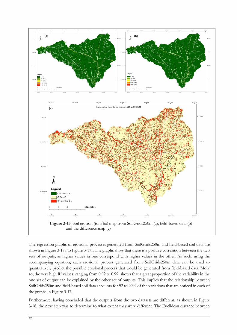
The modelled soil loss maps from both data sources and the difference map are shown in Figure 3-15a to

Figure 3-15c. Appendix 3-3 to Appendix 3-8 show the detachment by raindrops, detachment by runoff,

total detachment, runoff, runoff transport capacity and deposition maps generated from both data sources

and the respective difference maps.

For a large part of study area, the generated data were similar, while for other areas, the SoilGrids250m data

generated higher values (Appendix 3-5c and Figure 3-15c). On the other hand, Appendix 3-8c shows that

unlike detachment (Appendix 3-5c) and erosion (Figure 3-15c), while a large portion of the area still had

relatively similar sediment deposition predictions and a major portion of the remaining area still recorded

higher deposition estimates for SoilGrids250m data, a large portion recorded higher values for field-based

data. The predominant trend, as shown in the detachment by raindrops (Appendix 3-3), detachment by

runoff (Appendix 3-4), runoff (Appendix 3-6) and runoff transport capacity (Appendix 3-7) maps are in line

with those of detachment (Appendix 3-5) and erosion (Figure 3-15). This may be attributed to the fact as

shown in Figure 3-12a to Figure 3-12e and Figure 3-13a to Figure 3-13e that the values of the soil

characteristics represented in SoilGrids250m data were consistently higher than the field-based data, with

the singular exception of silt content. Statistical analysis was subsequently conducted to determine whether

the difference between the two set of outputs are statistically significant.

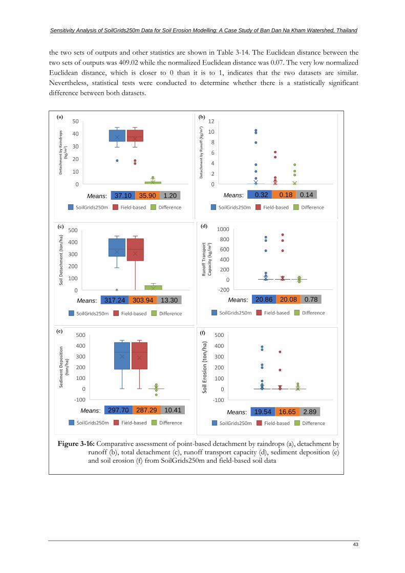
A. Point-based Assessment of the RMMF Model Outputs

The point-based field and SoilGrids250m output data, and the residual values after field-based values were

subtracted from SoilGrids250m-based values are shown in Figure 3-16a to Figure 3-16f. The figures show

that unlike the case of the inputs where the field-based data consistently seemed to have a greater degree of

variability than the SoilGrids250m data, the range and variability of the output data were relatively similar.

This gives the impression that the outputs from both data sources may not be very different from each

other. This is attributable to the fact that soil data is not the only input data used in the RMMF model. The

integrated effect of the land cover and rainfall inputs played a key role in homogenizing the variability.

Total detachment for SoilGrids250m and field-based data are 317 and 304 ton/ha respectively, with a mean

difference of 13 ton/ha (Figure 3-16c). Sediment deposition for SoilGrids250m and field-based data are 298

and 287 ton/ha respectively, with a mean difference of 10 ton/ha (Figure 3-16e). Soil erosion for

SoilGrids250m and field-based data are 20 and 17 ton/ha respectively, with a mean difference of 3 ton/ha

(Figure 3-16f). Similar trends were recorded for all other erosional processes. The difference between the

outputs seem conservative, even though in reality, it may make a lot of difference. This informed the need

to assess these data further to determine whether the modelled output from one dataset can be used to

predict the output from the other dataset. SoilGrids250m data is currently available and has a global

coverage, while field data may need to be generated whenever the need arises. The question then arises as

to whether we can use the modelled values from SoilGrids250m to predict the values of the different

erosional processes that would have been generated if field-based data were used instead of SoilGrids250m

data.

42

The regression graphs of erosional processes generated from SoilGrids250m and field-based soil data are

shown in Figure 3-17a to Figure 3-17f. The graphs show that there is a positive correlation between the two

sets of outputs, as higher values in one correspond with higher values in the other. As such, using the

accompanying equation, each erosional process generated from SoilGrids250m data can be used to

quantitatively predict the possible erosional process that would be generated from field-based data. More

so, the very high R2 values, ranging from 0.92 to 0.99, shows that a great proportion of the variability in the

one set of output can be explained by the other set of outputs. This implies that the relationship between

SoilGrids250m and field-based soil data accounts for 92 to 99% of the variations that are noticed in each of

the graphs in Figure 3-17.

Furthermore, having concluded that the outputs from the two datasets are different, as shown in Figure

3-16, the next step was to determine to what extent they were different. The Euclidean distance between


Figure 3-15: Soil erosion (ton/ha) map from SoilGrids250m (a), field-based data (b) and the difference map (c)

(a) (b)

(c)


43

the two sets of outputs and other statistics are shown in Table 3-14. The Euclidean distance between the

two sets of outputs was 409.02 while the normalized Euclidean distance was 0.07. The very low normalized

Euclidean distance, which is closer to 0 than it is to 1, indicates that the two datasets are similar.

Nevertheless, statistical tests were conducted to determine whether there is a statistically significant

difference between both datasets.

Figure 3-16: Comparative assessment of point-based detachment by raindrops (a), detachment by

runoff (b), total detachment (c), runoff transport capacity (d), sediment deposition (e) and soil erosion (f) from SoilGrids250m and field-based soil data

Means: 37.10 35.90 1.20

Means: 0.32 0.18 0.14

Means: 317.24 303.94 13.30

Means: 20.86 20.08 0.78

Means: 297.70 287.29 10.41

Means: 19.54 16.65 2.89

(a) (b)

(c) (d)

(e) (f)

44

The skewness and kurtosis z-value for several of the parameters (at P>0.05) were outside the range of -1.96

and +1.96 and their Shapiro-Wilk P-value were also consistently less than 0.05 (Table 3-14). This indicates

that most of the output parameters for both data sources are not normally distributed. Nevertheless, a

y = 0.9453x + 0.8264R² = 0.9237

0

5

10

15

20

25

30

35

40

45

50

0 20 40 60

Fiel

d D

ata

SoilGrids Data

Soil Detachment by Raindrops (kg/m2)

y = 0.6102x - 0.0143R² = 0.9825

-1

0

1

2

3

4

5

6

7

0 5 10 15

Fiel

d D

ata

SoilGrids Data

Soil Detachment by Runoff (kg/m2)

y = 0.9577x + 0.2546R² = 0.9819

0

100

200

300

400

500

0 200 400 600

Fiel

d D

ata

SoilGrids Data

Soil Detachment (ton/ha)

y = 1.0182x - 1.1291R² = 0.994

-200

0

200

400

600

800

1000

0 200 400 600 800 1000

Fiel

d D

ata

SoilGrids Data

Runoff Transport Capacity (kg/m2)

y = 0.9567x + 2.4334R² = 0.9844

0

100

200

300

400

500

0 200 400 600

Fiel

d D

ata

SoilGrids Data

Sediment Deposition (ton/ha)

y = 0.9085x - 1.0707R² = 0.9914

-50

0

50

100

150

200

250

300

350

400

0 100 200 300 400 500

Fiel

d D

ata

SoilGrids Data

Soil Erosion (ton/ha)

Figure 3-17: Regression analysis of point-based detachment by raindrops [kg/m2] (a), detachment by runoff [kg/m2] (b), total detachment [ton/ha] (c), runoff transport capacity [kg/m2] (d), sediment deposition [ton/ha] (e) and soil erosion [ton/ha] (f) from SoilGrids250m and field-based soil data

(a) (b)

(c) (d)

(e) (f)


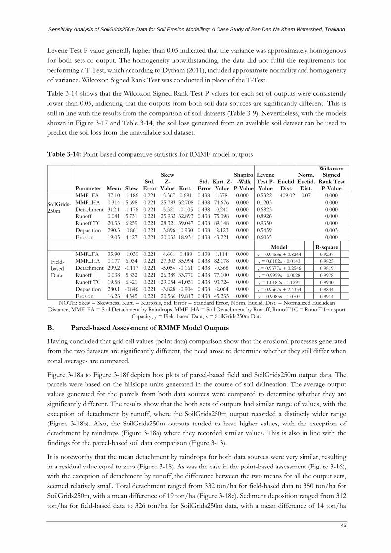
45

Levene Test P-value generally higher than 0.05 indicated that the variance was approximately homogenous

for both sets of output. The homogeneity notwithstanding, the data did not fulfil the requirements for

performing a T-Test, which according to Dytham (2011), included approximate normality and homogeneity

of variance. Wilcoxon Signed Rank Test was conducted in place of the T-Test.

Table 3-14 shows that the Wilcoxon Signed Rank Test P-values for each set of outputs were consistently

lower than 0.05, indicating that the outputs from both soil data sources are significantly different. This is

still in line with the results from the comparison of soil datasets (Table 3-9). Nevertheless, with the models

shown in Figure 3-17 and Table 3-14, the soil loss generated from an available soil dataset can be used to

predict the soil loss from the unavailable soil dataset.

Table 3-14: Point-based comparative statistics for RMMF model outputs


Error

Skew Z-

Value Kurt. Std.

Error Kurt. Z-Value

Shapiro-Wilk

P-Value

Levene Test P-Value

Euclid. Dist.

Norm. Euclid.

Dist.

Wilkoxon Signed

Rank Test P-Value

SoilGrids-250m

MMF_FA 37.10 -1.186 0.221 -5.367 0.691 0.438 1.578 0.000 0.5322 409.02 0.07 0.000

MMF_HA 0.314 5.698 0.221 25.783 32.708 0.438 74.676 0.000 0.1203 0.000

Detachment 312.1 -1.176 0.221 -5.321 -0.105 0.438 -0.240 0.000 0.6823 0.000

Runoff 0.041 5.731 0.221 25.932 32.893 0.438 75.098 0.000 0.8926 0.000

Runoff TC 20.33 6.259 0.221 28.321 39.047 0.438 89.148 0.000 0.9350 0.000

Deposition 290.3 -0.861 0.221 -3.896 -0.930 0.438 -2.123 0.000 0.5459 0.003

Erosion 19.05 4.427 0.221 20.032 18.931 0.438 43.221 0.000 0.6035 0.000

Model R-square

Field-based Data

MMF_FA 35.90 -1.030 0.221 -4.661 0.488 0.438 1.114 0.000 y = 0.9453x + 0.8264 0.9237 MMF_HA 0.177 6.034 0.221 27.303 35.994 0.438 82.178 0.000 y = 0.6102x - 0.0143 0.9825 Detachment 299.2 -1.117 0.221 -5.054 -0.161 0.438 -0.368 0.000 y = 0.9577x + 0.2546 0.9819 Runoff 0.038 5.832 0.221 26.389 33.770 0.438 77.100 0.000 y = 0.9959x - 0.0028 0.9978 Runoff TC 19.58 6.421 0.221 29.054 41.051 0.438 93.724 0.000 y = 1.0182x - 1.1291 0.9940

Deposition 280.1 -0.846 0.221 -3.828 -0.904 0.438 -2.064 0.000 y = 0.9567x + 2.4334 0.9844

Erosion 16.23 4.545 0.221 20.566 19.813 0.438 45.235 0.000 y = 0.9085x - 1.0707 0.9914

NOTE: Skew = Skewness, Kurt. = Kurtosis, Std. Error = Standard Error, Norm. Euclid. Dist. = Normalized Euclidean Distance, MMF_FA = Soil Detachment by Raindrops, MMF_HA = Soil Detachment by Runoff, Runoff TC = Runoff Transport

Capacity, y = Field-based Data, x = SoilGrids250m Data

B. Parcel-based Assessment of RMMF Model Outputs

Having concluded that grid cell values (point data) comparison show that the erosional processes generated

from the two datasets are significantly different, the need arose to determine whether they still differ when

zonal averages are compared.

Figure 3-18a to Figure 3-18f depicts box plots of parcel-based field and SoilGrids250m output data. The

parcels were based on the hillslope units generated in the course of soil delineation. The average output

values generated for the parcels from both data sources were compared to determine whether they are

significantly different. The results show that the both sets of outputs had similar range of values, with the

exception of detachment by runoff, where the SoilGrids250m output recorded a distinctly wider range

(Figure 3-18b). Also, the SoilGrids250m outputs tended to have higher values, with the exception of

detachment by raindrops (Figure 3-18a) where they recorded similar values. This is also in line with the

findings for the parcel-based soil data comparison (Figure 3-13).

It is noteworthy that the mean detachment by raindrops for both data sources were very similar, resulting

in a residual value equal to zero (Figure 3-18). As was the case in the point-based assessment (Figure 3-16),

with the exception of detachment by runoff, the difference between the two means for all the output sets,

seemed relatively small. Total detachment ranged from 332 ton/ha for field-based data to 350 ton/ha for

SoilGrids250m, with a mean difference of 19 ton/ha (Figure 3-18c). Sediment deposition ranged from 312

ton/ha for field-based data to 326 ton/ha for SoilGrids250m data, with a mean difference of 14 ton/ha

46

(Figure 3-18e). Soil loss ranged from 20 ton/ha for field-based data to 24 ton/ha for SoilGrids250m data

(Figure 3-18f). Consequently, as was the case with the point-based assessment, the data required further

analysis.

Table 3-15 shows the data generated from further quantitative analysis of the model outputs. The Euclidean

distance between the two sets of outputs was 70.90 while the normalized Euclidean distance was 0.03. Even

though the Euclidean distance is much lower that the value (409.02) recorded during the point-based

assessment, the normalized Euclidean distance was still very close to the value (0.07) reported for point-

based assessment. This may be attributed to the fact that irrespective of the fact that the number of values

being compared are different, the datasets are still the same. The very low normalized Euclidean distance,

corroborates the results from the point-based assessment, indicating that the datasets similar.

To determine whether the difference was statistically significant for the other sets of outputs T-Test was

calculated for each set. The skewness z-value, kurtosis z-value and Shapiro-Wilk P-value, all indicated that

Mean: 36.73 36.73 0.00

Mean: 0.420 0.708 0.288

Mean: 331.54 350.23 18.69

Mean: 53.59 55.74 2.15

Mean: 311.60 325.77 14.45

Mean: 19.94 24.46 4.52

Figure 3-18: Comparative assessment of parcel-based detachment by raindrops (a), detachment by runoff (b), total detachment (c), runoff transport capacity (d), sediment deposition (e) and soil erosion (f) from SoilGrids250m and field-based soil data

(a) (b)

(c) (d)

(e) (f)


47

both sets of outputs are approximately normal (Table 3-15). Similarly, the Levene Test, with P-values

consistently higher than 0.05 (Table 3-15), indicated that all the output data has approximately homogenous

variability. They consequently met the requirements for implementing the T-Test, as documented by

Dytham (2011).

The T-Test P-values (Table 3-15) show that at P>0.05, the estimates for detachment by raindrops, total

detachment and deposition were not significantly different for both datasets; at P>0.01, the estimates for

detachment by runoff, runoff and runoff transport capacity were not significantly different. However, a P-

value of 0.005, indicates that the erosion data generated from the two data sources were significantly

different.

Table 3-15: Hillslope parcel-based comparative statistics for RMMF model outputs

Parameter Mean Skew

Std.

Error

Skew

Z-

Value Kurtosis

Std.

Error

Kurtosis

Z-Value

Shapiro-

Wilk P-

Value

Levene

Test P-

Value

Euclid.

Dist.

Norm.

Euclid.

Dist.

T-Test

P-Value

SoilGrids-

250m

MMF_FA 37 -0.506 1.014 -0.499 1.438 2.619 0.549 0.824 1.000 70.90 0.03 ***

MMF_HA 0.708 -1.046 1.014 -1.032 0.969 2.619 0.370 0.674 0.398 0.023

Detachment 350 -1.491 1.014 -1.470 2.103 2.619 0.803 0.285 0.873 0.173

Runoff 0.038 0.533 1.014 0.526 -3.004 2.619 -1.147 0.281 0.880 0.041

Runoff TC 56 -0.930 1.014 -0.917 1.989 2.619 0.759 0.502 0.971 0.016

Deposition 326 -0.845 1.014 -0.833 0.240 2.619 0.092 0.781 0.740 0.281

Erosion 24 -0.434 1.014 -0.428 1.342 2.619 0.512 0.859 0.903 0.005

Field-

based

Data

MMF_FA 37 -0.506 1.014 -0.499 1.438 2.619 0.549 0.824

MMF_HA 0.420 -0.967 1.014 -0.954 1.921 2.619 0.733 0.616

Detachment 332 -1.427 1.014 -1.407 2.614 2.619 0.998 0.332

Runoff 0.035 0.477 1.014 0.470 -3.171 2.619 -1.211 0.393

Runoff TC 54 -0.807 1.014 -0.796 1.867 2.619 0.713 0.546

Deposition 312 -1.375 1.014 -1.356 2.102 2.619 0.803 0.429

Erosion 20 -0.196 1.014 -0.193 1.519 2.619 0.580 0.698 NOTE: Skew = Skewness, Kurt. = Kurtosis, Std. Error = Standard Error, Norm. Euclid. Dist. = Normalized Euclidean Distance, MMF_FA = Soil Detachment by Raindrops, MMF_HA = Soil Detachment by Runoff, Runoff TC = Runoff Transport Capacity, *** = Exactly the same values (could not be computed because the

standard error of the difference is 0)

Because erosion control or prevention may not usually target the erosion itself, but its predisposing factors,

the data from SoilGrids250m is still valuable. It can be used to target zones with excessive runoff, zones

with high detachment by raindrops, zones with high detachment by runoff and zones with high runoff

transport capacity. Soil conservation measures implemented in these zones will ultimately lead to reduced

soil loss. Similarly, it can be used to quantify the off-site effect of soil erosion as the sediment deposition

generated by both datasets were also very similar.

However, the fact that the erosional processes which were significantly different when point-based

assessment was done, turned out to be similar when parcel-based assessment was performed, has

implications relating to the scale at which the SoilGrid250m generated erosional processes can be applied in

soil conservation or land use planning. The SoilGrids250m-generated outputs are more useful for regional,

district or provincial soil conservation / land use planning, where very detailed estimates of the erosional

processes are not required. If more detailed, site-specific information are required, then, in the absence of

field-generated data, SoilGrids250m can be used to predict the annual extent of the erosional processes,

after which the models in Figure 3-17 and Table 3-14 can be used to predict the field-based estimates.

3.3.2. Assessment of the Sensitivity of the Model Parameters

The fifth and the sixth research questions were related to the determination of the soil and land cover

parameters that the modelled erosional processes are more sensitive to. The findings are discussed in this

48

section. Figure 3-19 to Figure 3-22 and Appendix 3-9 to Appendix 3-11 graphically depict the percent change

in the average predicted erosional processes in the watershed for every 20% increase in input parameters.

A. Sensitivity of Rainfall Parameters: Detachment by raindrops (Appendix 3-9), detachment by runoff

(Appendix 3-10), total detachment (Figure 3-19), runoff (Figure 3-20), runoff transport capacity

(Appendix 3-11) and soil erosion (Figure 3-22) were all more sensitive to rainfall amount than they are

to number of rainy days. Nevertheless, sediment deposition (Figure 3-21) appears to be marginally

more sensitive to number of rainy days as 100% increase in number of rainy days resulted in a 22%

increase in deposition, while a 100% increase in rainfall amount resulted in only 18% increase in

sediment deposition. This is in line with the findings of Morgan & Duzant (2008) that erosional

processes are more sensitive to rainfall amount. With regards to deposition, it seems odd that increase

in rainfall amount should result in increase in deposition. This apparent anomaly may be attributed to

the fact that as rainfall increases, detachment also increases, but since the runoff transport capacity is

low, the high detachment will also result in high deposition.

B. Sensitivity of Soil Parameters: Appendix 3-9 shows that besides soil erodibility, detachment by

raindrops was not sensitive to any other soil parameter. Indeed, a 100% increase in soil erodibility

equally results in a 100% increase in detachment by raindrops. One would, however, have expected

that detachment by raindrops would be sensitive to cohesion as cohesive soils are less easily detached

than non-cohesive soils. But the model does not seem to be sensitive to it. This is perhaps, due to the

contention of Mahalder et al. (2016) that prediction of cohesive soil erodibility is difficult because

credible models that capture its dynamics are currently not available. On the other hand, besides soil

erodibility, detachment by runoff (Appendix 3-10) was sensitive to all other soil parameters. It was,

however, most sensitive to moisture content at field capacity and effective hydrological depth. In both

cases, a 100% increase resulted in an 84% decrease in soil detachment by runoff. Figure 3-19 shows

that total detachment was most sensitive to soil erodibility, as it increased by 95% with 100% increase

in erodibility. It is noteworthy that total detachment is sensitive to all soil parameters, albeit, marginal

for field capacity, cohesion and effective hydrological depth. With respect to runoff estimate, it was

equally sensitive to moisture content at field capacity and effective hydrological depth, as a 100%

increase in any of them resulted in a 72% decrease in estimated runoff. Runoff was nonetheless, not

sensitive to cohesion and erodibility (Figure 3-20). Expectedly, runoff transport capacity was also not

sensitive to cohesion and erodibility, but equally sensitive to field capacity and effective hydrological

depth – runoff transport capacity decreases by 89% with every 100% increase in field capacity or

effective hydrological depth (Appendix 3-11). Figure 3-21 shows that sediment deposition is most

sensitive to soil erodibility, as 100% increase in soil erodibility results in up to 114% increase in

deposition. It was also sensitive to field capacity and effective hydrological depth, but not sensitive to

cohesion. With respect to soil erosion (Figure 3-22), moisture content at field capacity and effective

hydrological depth had the highest sensitivity of up to 80%, while cohesion had the least sensitivity of

7%. It is important to note that only soil erodibility had a position relationship with soil erosion; the

other parameters had an inverse relationship with soil erosion.

C. Sensitivity of Land Cover Parameters: Appendix 3-9 shows that detachment by raindrops was most

sensitive to water interception by vegetation (A), as 100% increase in interception results in a 66%

decrease in detachment by raindrops. It was also sensitive to canopy cover (CC) and plant height (PH),

as 100% increase in any of the variables results in over 25% increase in detachment by raindrops.

Detachment by raindrops was not sensitive to any of the other land cover parameters. Detachment by

runoff (Appendix 3-10) was most sensitive to the ratio of actual to potential evapotranspiration, which

had a sensitivity of 84%. This is in line with the findings of Morgan & Duzant (2008) that runoff is

highly sensitive to evapotranspiration. Detachment by runoff was also sensitive to interception by


49

vegetation and surface cover, but not sensitive to crop management factor, canopy cover and plant

height. Total detachment (Figure 3-19) was most sensitive to rainfall interception by vegetation with a

sensitivity of up to 53%. The only land cover parameter that it was not sensitive to was crop

management factor. Runoff estimate (Figure 3-20) was most sensitive to the ratio of actual to potential

evapotranspiration – which is in accord with the findings of Morgan & Duzant (2008) – with a

sensitivity of up to 72%. The only other land cover parameter it was sensitive to was interception by

vegetation. Runoff transport capacity (Appendix 3-11) was most sensitive to crop management factor,

which had a sensitivity of up to 100%. It was not sensitive to canopy cover, surface cover and plant

height. Sediment deposition (Figure 3-21) was most sensitive to interception by vegetation, with a

sensitivity of up to 52%. Besides surface cover, it was sensitive to all other parameters. Soil erosion

(Figure 3-22) was most sensitive to the ratio of actual to potential evapotranspiration, with a sensitivity

of up to 80%. It was sensitive to all land cover parameters, but least sensitive to canopy cover (7 %).

D. Overall Sensitivity: Appendix 3-9 shows that, overall, detachment by raindrops was most sensitive to

rainfall amount (100%) and soil erodibility (100%). Detachment by runoff (Appendix 3-10), total

detachment (Figure 3-19), runoff estimate (Figure 3-20), runoff transport capacity (Appendix 3-11)

and soil erosion (Figure 3-22), were all most sensitive to changes in rainfall amount. The only parameter

that was an exception was soil deposition (Figure 3-21), which was most sensitive to soil erodibility

(114%). The findings of this study is in line with those of Morgan & Duzant (2008), which were

reiterated by Choi et al. (2016), that soil loss and runoff estimates are most sensitive to variations in

rainfall amount. Furthermore, Morgan & Duzant (2008) asserted that for bare soils, besides rainfall,

the MMF model estimates of soil loss is more sensitive to soil parameters, but that with increase in

vegetation cover, land cover becomes progressively more important. They, however, also stated that

irrespective of the vegetation cover or the lack of it, in addition to rainfall, runoff was also sensitive to

soil moisture storage (soil moisture content at field capacity and effective hydrological depth) and

evapotranspiration (ratio of actual to potential evapotranspiration) as was also evident in Figure 3-20.

-100.00

-50.00

0.00

50.00

100.00

150.00

200.00

RF RD MS K COH EHD Et/Eo C A CC SC PH

Climate Soil Land Cover% C

han

ge in

To

tal D

etac

hm

ent

per

20%

P

aram

etri

c In

crea

se

20% 40% 60% 80% 100%

Figure 3-19: Sensitivity of total soil detachment to various input parameters

RF = Rainfall (mm), RD = Rainy Days, MS = Field Capacity (%), K = Erodibility (kg/J), COH = Cohesion (kPa), EHD = Effective Hydrological Depth (m), Et/Eo = Ratio of Actual to Potential Evapotranspiration, C = Crop Management Factor, A = Rainfall Interception by Vegetation (mm), CC = Canopy Cover

(%), SC = Surface Cover (%), PH = Plant Height (m)

50

-100.00

-50.00

0.00

50.00

100.00

150.00

200.00



han

ge in

Ru

no

ff E

stim

ate

per

20

%

Par

amet

ric

Incr

ease

20% 40% 60% 80% 100%

-80.00

-60.00

-40.00

-20.00

0.00

20.00

40.00

60.00

80.00

100.00

120.00

140.00


Climate Soil Land Cover

% C

han

ge in

Sed

imen

t D

epo

siti

on

per

20%

P

aram

etri

c In

crea

se

20% 40% 60% 80% 100%

Figure 3-20: Sensitivity of runoff estimate to various input parameters



Figure 3-21: Sensitivity of sediment deposition to various input parameters




51

3.3.3. Assessment of the Spatial Extent of Soil Erosion within the Different Land Cover and Slope Units of the Watershed

The seventh and eight research questions focussed on the assessment of which land cover and hillslope

units are more prone to soil erosion. It is noteworthy that field assessment of erosional processes within the

study area could not be conducted. Similarly, secondary validation data was also not available. Nevertheless,

Morgan (2001) validated the runoff and soil loss generated by the RMMF model for 91 sites in 17 different

countries, including Thailand. The findings of the assessment of the erosional processes in the study area

are discussed in this section. The output data are presented in maps, tables and graphs.

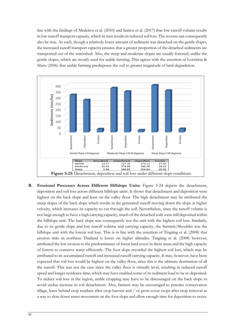
A. Erosional Processes Under Different Slope Conditions: Figure 3-23 depicts the detachment,

deposition and soil loss from different slope units. Figure 3-23 shows that soil detachment was highest

in the steep slopes (399 ton/ha/annum) and least in the gentle slopes (317 ton/ha/annum). Soil loss,

which ranges from 18 to 30 ton/ha/annum, was however, much lower than detachment. This may be

attributed to the low runoff volume (Table 3-16), which in turns translated into low runoff transport

capacity (Table 3-16). Because the runoff does not have the capacity to transport the detached

sediments out of the watershed, a very large proportion of the detached sediments are re-deposited

within the vicinity of the area from which they were detached. This was why the deposition is also

quite high (274 to 354 ton/ha/annum), almost at par with detachment. Given the relatively high rate

of detachment on steep slopes, land uses, like arable farming, that may predispose the soil to the direct

impact of raindrops and runoff, ought to be discouraged on steep slopes. Ideally, it would have been

expected that soil loss would be highest on the steep slope, but it turned out to be highest on the gentle

slopes. This may be attributed to the fact that all the runoff from the steep and moderate slopes get

accumulated on the gentle slopes, increasing runoff volume and runoff transport capacity. This is in

-200.00

-100.00

0.00

100.00

200.00

300.00

400.00

500.00

600.00



han

ge in

So

il Lo

ss E

stim

ate

per

20

% P

aram

etri

c In

crea

se

20% 40% 60% 80% 100%

Figure 3-22: Sensitivity of soil loss estimation to various input parameters



52

line with the findings of Medeiros et al. (2010) and Santos et al. (2017) that low runoff volume results

in low runoff transport capacity, which in turn results in reduced soil loss. The reverse can consequently

also be true. As such, though a relatively lower amount of sediment was detached on the gentle slopes,

the increased runoff transport capacity ensures that a greater proportion of the detached sediments are

transported out of the watershed. Also, the steep and moderate slopes are usually forested, unlike the

gentle slopes, which are mostly used for arable farming. This agrees with the assertion of Lorsirirat &

Maita (2006) that arable farming predisposes the soil to greater magnitude of land degradation.

B. Erosional Processes Across Different Hillslope Units: Figure 3-24 depicts the detachment,

deposition and soil loss across different hillslope units. It shows that detachment and deposition were

highest on the back slope and least on the valley floor. The high detachment may be attributed the

steep slopes of the back slope which results in the generated runoff moving down the slope at higher

velocity, which increases its capacity to cut through the soil. Nevertheless, since the runoff volume is

not large enough to have a high carrying capacity, much of the detached soils were still deposited within

the hillslope unit. The back slope was consequently not the unit with the highest soil loss. Similarly,

due to its gentle slope and low runoff volume and carrying capacity, the Summit/Shoulder was the

hillslope unit with the lowest soil loss. This is in line with the assertion of Tingting et al. (2008) that

erosion risks in northern Thailand is lower on higher altitudes. Tingting et al. (2008) however,

attributed the low erosion to the predominance of forest land cover in these areas and the high capacity

of forests to conserve water efficiently. The foot slope recorded the highest soil loss, which may be

attributed to its accumulated runoff and increased runoff carrying capacity. It may, however, have been

expected that soil loss would be highest on the valley floor, since this is the ultimate destination of all

the runoff. This was not the case since the valley floor is virtually level, resulting in reduced runoff

speed and longer residence time, which may have enabled some of its sediment load to be re-deposited.

To reduce soil loss in the region, arable cropping may have to be discouraged on the back slope to

avoid undue increase in soil detachment. Also, farmers may be encouraged to practice conservation

tillage, leave behind crop residues after crop harvest and / or grow cover crops after crop removal as

a way to slow down water movement on the foot slope and allow enough time for deposition to occur.

0

50

100

150

200

250

300

350

400

Det

ach

me

nt

Dep

osi

tio

n

Ero

sio

n

Det

ach

me

nt

Dep

osi

tio

n

Ero

sio

n

Det

ach

me

nt

Dep

osi

tio

n

Ero

sio

n

Gentle Slope (<8 degrees) Moderate Slope (<8-30 degrees) Steep Slope (>30 degrees)

Sed

ime

nts

(to

n/h

a)

Figure 3-23: Detachment, deposition and soil loss under different slope conditions


53

C. Erosional Processes Under Different Land Cover Types: Figure 3-25 depicts the detachment,

deposition and soil loss under the various land cover types delineated in the watershed. It shows that

detachment and deposition were highest in teak plantations (416 and 403 ton/ha respectively) and least

on arable soils (185 and 115 ton/ha respectively). The relatively high detachment in forests and teak

plantation may be attributed to the predominance of tall trees in both land cover types, which invariably

increases detachment by raindrops (leaf drainage). Detachment by raindrops was, however, much more

severe in teak plantations due to the virtual nonexistence of undergrowth in the plantation, unlike was

the case in forests. This may have informed the higher detachment in teak plantations as Labrière et

al. (2015) asserted that in the humid tropics, soil loss is highest when there is no extra vegetation layer

under the forest canopy. Similarly, Tingting et al. (2008) also contended that plantations are relatively

more prone to erosion. Consequently, the cultivation of shade-loving plants under the canopy of the

teak trees may be recommended, especially for regions on steep slopes. However, even though

detachment was least on arable lands, soil loss was highest – as high as 69 ton/ha. This is in line with

the contention of Lorsirirat & Maita (2006) that in Northern Thailand, agricultural practices predispose

the soils to erosion. This may be attributed to increased runoff and runoff carrying capacity in the foot

slope and valley floor where most of the arable lands are located. In addition to that, agricultural

practices that lead to the soil being bare for prolonged periods of time may also be a contributory

factor.

050

100150200250300350400

Det

ach

men

t

Dep

osi

tio

n

Soil

Loss

Det

ach

men

t

Dep

osi

tio

n

Soil

Loss

Det

ach

men

t

Dep

osi

tio

n

Soil

Loss

Det

ach

men

t

Dep

osi

tio

n

Soil

Loss

Summit/Shoulder Back Slope Foot Slope Valley Floor

Sed

ime

nt

(to

n/h

a)

0

100

200

300

400

500

Det

ach

men

t

Dep

osi

tio

n

Ero

sio

n

Det

ach

men

t

Dep

osi

tio

n

Ero

sio

n

Det

ach

men

t

Dep

osi

tio

n

Ero

sio

n

Det

ach

men

t

Dep

osi

tio

n

Ero

sio

n

Arable Land Orchard Forest Teak Plantation

Sed

ime

nts

(to

n/h

a)

Figure 3-24: Detachment, deposition and soil loss across different hillslope units

Figure 3-25: Detachment, deposition and soil loss under different land use types

54

D. Erosional Processes Under Different Land Cover-Slope Units: Figure 3-26 shows a map of the

study area, depicting the location and extent of the various land use types under different slope

conditions, while Table 3-16 shows the predicted values of the erosional processes taking place in each

unit. Table 3-16 shows that for each land cover type, detachment was highest on the steep slopes and

least on the gentle slopes. Overall, it was highest on teak plantation soils on steep slopes (431 ton/ha)

and least on arable soils on gentle slopes (169 ton/ha). Due the relatively low runoff volume and

transport capacity, deposition followed the same trends as did detachment. The exception to the rule

was the arable lands, where deposition was highest on the gentle slopes and lowest on steep slopes.

This may be attributed to the fact that the gentle slopes allowed enough time for the accumulated

runoff to deposit a relatively larger proportion of its sediment load, a phenomenon that is not feasible

on steep slopes. Figure 3-27 depicts the soil loss across the land cover-slope units of the watershed. It

shows that though total detachment was lowest on arable lands (Table 3-16), soil loss was highest,

ranging from 46 ton/ha on gentle slopes to 132 ton/ha on steep slopes. This is in line with the assertion

of Tingting et al. (2008) that arable soils, especially those on steep slopes, are very prone to erosion.

Similarly, Vlassak et al. (1993), Panomtaranichagul et al. (2002), Panomtaranichagul & Nareuban (2005)

and Wicharuck et al. (2010) contended that agricultural activities on the highlands of northern Thailand

results in 5 to 297 ton/ha soil loss per annum. The high soil loss is attributable to the land use type,

which does not protect the soil adequately and the increased runoff and runoff transport capacity on

moderate to gentle slopes. The lower soil loss on gentle slopes for all land use types may be attributed

to the relatively lower runoff velocity and energy on gentle slopes, and the increased residence time,

which permits a greater degree of deposition.

Furthermore, with regards to the soil loss tolerance, Hudson (1981) and Morgan (2005) reported that

a mean annual soil loss of 11 ton/ha is generally considered acceptable for soils that are up to 1m deep,

but that the acceptable soil loss can be as low as 2 t/ha for sensitive areas where soils are thin or highly

erodible. It has also been recommended that in regions where soils are over 2m deep, the soil loss

tolerance can be increased to 15 – 20 ton/ha (Schertz, 1983; Morgan, 2005). Therefore, with a soil loss

ranging from 6.5 ton/ha for gentle slopes to 10.48 ton/ha for steep slopes, soil loss in forest is still

within the acceptable range. With respect to orchards, only those on gentle slopes had soil losses (9.11

ton/ha) within the tolerable limit of less than 11 ton/ha. Nevertheless, because most of the soils of

the watershed are deep, and the soil loss for both moderate slope (14.93 ton/ha) and steep slope (18.16

ton/ha) are still less than 20 ton/ha, the predicted soil loss may be acceptable. Notwithstanding that

the soil loss is below 20 ton/ha, it is still important to implement some soil conservation measure,

particularly on steep slopes.

Teak plantations on both gentle (12.36 ton/ha) and moderate slopes (12.65 ton/ha) had soil loss values

exceeding 11 ton/ha, but because it was just marginally higher and very much less than 15 ton/ha, teak

can still be sustainably grown under these slope conditions. The planting of shade-loving plants under

the dense canopy of the teak trees may improve the situation further. On the other hand, with a soil

loss of 22.52 ton/ha, teak plantations on steep slopes exceed the maximum acceptable soil loss

tolerance. Establishing teak plantations on steep slopes may consequently be discouraged. If they must

be established, then soil conservation measures that reduce detachment and soil loss should be

implemented as a precondition for establishing the plantations.

Irrespective of the condition of the slope, soil loss on arable lands, by far, exceed the maximum

acceptable soil loss of 20 ton/ha. Arable farming on steep slopes, with a soil loss of up to 131.61

ton/ha should be outrightly discouraged. If arable farming is to be implemented on the moderate

slopes, then soil conservation measures like terracing (with hedge plants or trees along the contours),

should first be put in place. On gentle slopes, the soil loss was still as high as 45.67 ton/ha.


55

Consequently, even on gentle slopes, soil conservation measures and farming practices that discourage

soil degradation by reducing the period during which the soil is bare, reducing runoff velocity,

increasing runoff residence time and organic matter content, should be practiced.

Table 3-16: Soil erosion processes in the different landscape units of the watershed

Landscape Unit Area

(km2)

MMF_FA

(kg/m2)

MMF_HA

(kg/m2)

MMF_Det

(ton/ha)

RF

(mm)

MMF_TC

(kg/m2)

MMF_Dep

(ton/ha)

Erosion

(ton/ha)

AL-Gentle (< 8o) 2.49 18.521 0.920 169.494 0.106 115.831 123.820 45.67

AL-Moderate (8-30o) 3.16 18.233 1.780 192.747 0.098 172.935 110.940 81.81

AL-Steep (> 30o) 0.34 18.289 4.041 218.851 0.097 520.552 87.238 131.61

OR-Gentle (< 8o) 3.39 33.214 0.044 266.405 0.008 8.192 257.297 9.11

OR-Moderate (8-30o) 19.82 33.343 0.151 311.320 0.008 29.055 296.392 14.93

OR-Steep (> 30o) 1.61 33.397 0.179 325.807 0.008 33.017 307.651 18.16

FO-Gentle (< 8o) 4.97 41.897 0.070 356.170 0.000 1.543 349.669 6.50

FO-Moderate (8-30o) 30.25 41.992 0.146 396.948 0.000 3.294 389.599 7.35

FO-Steep (8-30o) 3.10 42.021 0.284 409.206 0.000 7.725 398.728 10.48

TP-Gentle (< 8o) 2.08 44.200 0.189 387.661 0.001 3.746 375.299 12.36

TP-Moderate (8-30o) 9.22 44.098 0.295 420.820 0.001 4.649 408.170 12.65

TP-Steep (> 30o) 0.92 44.132 0.674 430.527 0.001 12.049 408.004 22.52

NOTE: MMF_FA = Detachment by Raindrops (kg/m2), MMF_HA = Detachment by Runoff (kg/m2), RF = Runoff (mm), MMF_TC = Runoff

Transport Capacity (kg/m2), MMF_Det = Total Soil Detachment (ton/ha), MMF_Dep = Sediment Deposition (ton/ha), Erosion = Soil Erosion

(ton/ha), AL-Gentle = Arable Land on Gentle Slopes, AL-Moderate = Arable Land on Moderate Slopes, AL-Steep = Arable Land on Steep

Slopes, OR-Gentle = Orchards on Gentle Slopes, OR-Moderate = Orchards on Moderate Slopes, OR-Steep = Orchards on Steep Slopes, FO-

Gentle = Forests on Gentle Slopes, FO-Moderate = Forests on Moderate Slopes, FO-Steep = Forests on Steep Slopes, TP-Gentle = Teak

Plantations on Gentle Slopes, TP-Moderate = Teak Plantations on Moderate Slopes, TP-Steep = Teak Plantations on Steep Slopes

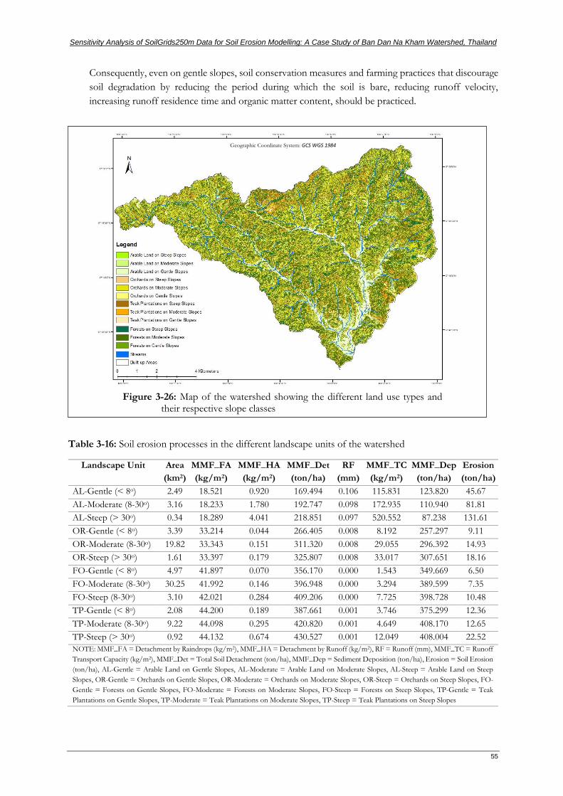
Figure 3-26: Map of the watershed showing the different land use types and their respective slope classes


56

0.00

20.00

40.00

60.00

80.00

100.00

120.00

140.00So

il Lo

ss (

ton

/ha)

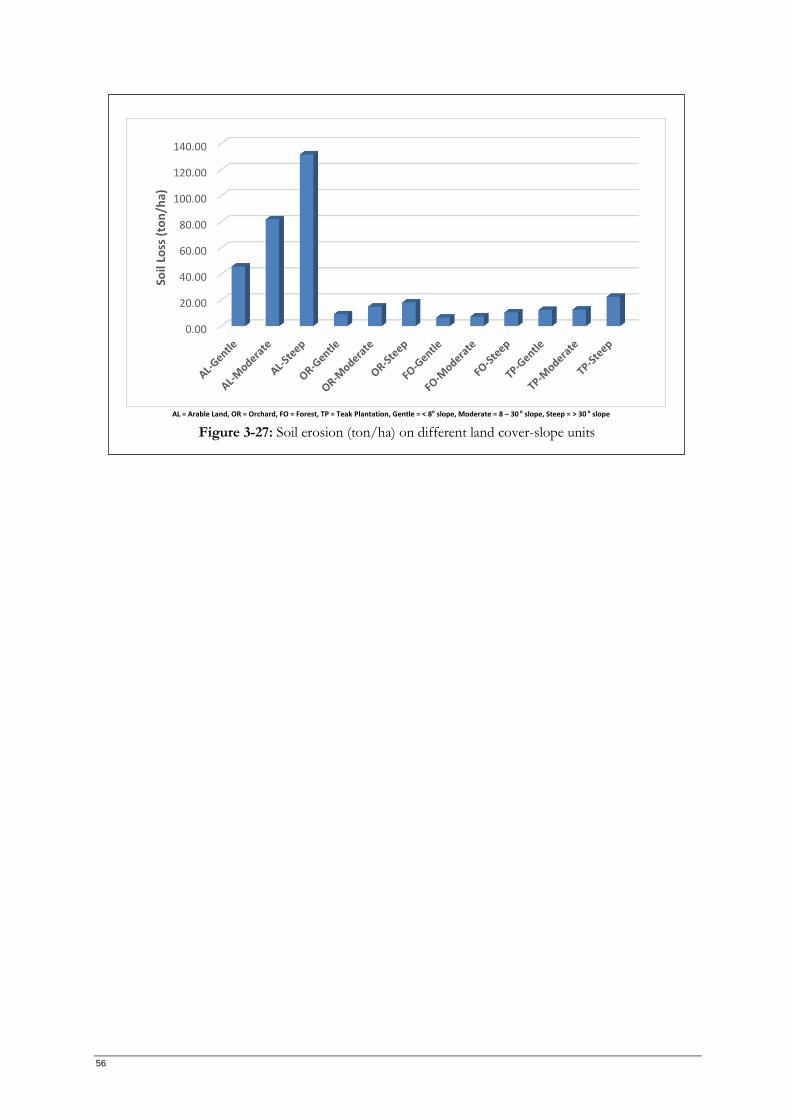
Figure 3-27: Soil erosion (ton/ha) on different land cover-slope units

AL = Arable Land, OR = Orchard, FO = Forest, TP = Teak Plantation, Gentle = < 8o slope, Moderate = 8 – 30 o slope, Steep = > 30 o slope


57

4. CONCLUSION AND RECOMMENDATIONS

4.1. Conclusion

Soil erosion is a global phenomenon that is more preponderant in the humid tropics, especially soil erosion

by water. Given its devastating off-site and on-site impacts, there has over the years, been a consensus that

it should be built into land evaluation and land use planning projects. As such, soil erosion assessment is a

necessary prerequisite to sustainable natural resources management. The acquisition of the input data for

the modelling is, however, time-consuming and capital-intensive. This is more so for soil survey data, which

requires extensive fieldwork. SoilGrids250m, which is available at a global scale, could potentially solve the

problem relating to the scarcity of soil data for erosion assessment. This study consequently assessed the

value of SoilGrids250m data for erosion modelling, relative to field-generated soil data.

The comparative assessment of the SoilGrids250m and the field-based soil data was performed at two scales

– point and areal. Point-based assessment indicated that the two soil datasets are significantly different. The

only exception to this rule was clay content, for which both datasets were not significantly different. On the

other hand, for the area-based assessment – which was based on the parametric average values of both

datasets for each of the delineated hillslope units in the study area – only silt content was significantly

different at P>0.01. All the other soil parameters were similar for both datasets. It may consequently be

concluded that for regional studies, which require the average soil property for delineated areal units,

SoilGrids250m data may be a good alternative to field data.

After assessing soil erosion for the study area using both datasets, the outputs relating to the erosional

processes (detachment by raindrops, detachment by runoff, total detachment, runoff, runoff transport

capacity, deposition and soil loss) were also compared to determine the extent of their similarities. As was

the case with the point-based assessment of the soil datasets, the point-based assessment of the model

outputs show that all the outputs generated were significantly different. Similarly, just like the area-based

assessment of the input data, the assessment of the outputs show that they are not significantly different at

P>0.01, with the exception of soil loss, for which the soil loss modelled from the SoilGrids250m was

significantly higher. This also implies that when planning land evaluation or soil conservation projects at a

regional scale areal averages of runoff and detachment from SoilGrids250m data may be adequate.

Nevertheless, for more site-specific erosion assessment in Northern Thailand, if time and funds are not

available for the acquisition of additional field data, SoilGrids250m data can be used to assess soil erosion.

Subsequently, using the models generated in this study, expected erosional processes from field-based data

can be predicted. It is also noteworthy that all erosional processes generated from the RMMF, besides

sediment deposition, were most sensitive to rainfall amount. Sediment deposition was most sensitive to soil

erodibility. Also, besides rainfall, soil loss estimate was quite sensitive to soil parameters (moisture content

at field capacity and effective hydrological depth) and land cover parameters (ratio of actual to potential

evapotranspiration and rainfall interception by vegetation). Extra care should consequently be taken when

running the RMMF model to ensure that these input parameters are of good quality.

Finally, the hillslope unit that is most susceptible to the forces of detachment (raindrop and runoff) is the

back slope, but the low runoff transport capacity makes it less susceptible to soil loss than the foot slope

which has lower detachment but greater soil loss. Slope classes below 8o are less prone to soil loss than other

slope classes. The land cover type most susceptible to erosion in the study area was the arable lands, while

forests were least susceptible.

58

4.2. Limitations

Some of the limitations encountered in the course of this study are:

- Lack of data for the validation of the RMMF model outputs.

- Inability to acquire a fine resolution DEM that will enable more accurate soil delineation.

- Inability to acquire a detailed geologic maps of the area, which would have been a necessary tool

for proper delineation of the soil map units.

- Available hillslope delineation algorithms were designed to use high resolution terrain data, like

LiDAR DEM or the airborne laser-derived DEM, which are usually not available in developing

countries

- The ruggedness of the terrain, which made it difficult to access of the pre-defined sample sites.

4.3. Recommendations

In terms of the methods, if similar studies are to be conducted, it may be necessary to delineate the hillslope

units prior to the fieldwork. The soil sampling scheme should be based on the delineated hillslope units.

This would eliminate the ambiguity inherent in trying to compare two sets of outputs that are not

comparable. With regards to the findings of this study, it is recommended that:

- Arable farming should be discouraged on steep and moderate slopes. Even on gentle slopes, arable

farming should be accompanied by sustainable soil conservation practices.

- The establishment of teak plantations and orchards on steep slopes should be discouraged; and the

implementation of land conservation measures should be a precondition for establishing teak

plantations or orchards on moderate slopes.

- Shade-loving plants may need to be grown in teak plantations to reduce soil detachment and soil

loss, and increase deposition by obstructing the flow of runoff.

4.4. Further Studies

In terms of the outcome of this study, some of the areas that require further research are:

- Validation of the outputs of the RMMF model for the watershed through field measurements of

runoff, soil loss and / or other erosional processes.

- Assessment of the value of SoilGrids250m data for daily soil erosion modeling.

- Generation of soil loss tolerance and other indices that can be used as a baseline to determine the

extent of soil loss that is acceptable in the region.

- Downscaling of soil delineation algorithms to permit the use of coarse resolution DEM (which are

available for developing countries) to generate hillslope units that effectively reflect the soil-

landscape relationship.


59

LIST OF REFERENCES

Alexakis, D. D., Hadjimitsis, D. G., & Agapiou, A. (2013). Integrated Use of Remote Sensing, GIS and Precipitation Data for the Assessment of Soil Erosion Rate in the Catchment Area of “ Yialias ” in Cyprus. Atmospheric Research, 131, 108–124.

Avwunudiogba, A., & Hudson, P. F. (2014). A Review of Soil Erosion Models with Special Reference to the needs of Humid Tropical Mountainous Environments. European Journal of Sustainable Development, 3(4), 299–310. https://doi.org/10.14207/ejsd.2014.v3n4p299

Baartman, J. E. M., Jetten, V. G., Ritsema, C. J., & Vente, J. (2012). Exploring Effects of Rainfall Intensity and Duration on Soil Erosion at the Catchment Scale Using openLISEM: Prado Catchment, SE Spain. Hydrological Processes, 26(7), 1034–1049. https://doi.org/10.1002/hyp.8196

Balan, A., Raus, L., & Jitareanu, G. (2009). Effects of Tillage Management on Soil Porosity and Bulk Density on Rape Effects of Tillage Management on Soil Porosity and Bulk Density on Rape ( Brasica Napus ). Bulletin UASVM Agriculture, 66(1), 260–263.

Beasley, D. B., Huggins, L. F., & Monke, E. J. (1980). Answers - A Model for Watershed Planning. Transactions of the ASAE, 23, 938–944.

Bhadha, J. H., Capasso, J. M., Khatiwada, R., Swanson, S., & LeBorde, C. (2017). Raising Soil Organic Matter Content to Improve Water Holding Capacity. Gainesville: University of Florida Institute of Food and Agricultural Sciences. Retrieved from http://edis.ifas.ufl.edu.

Choi, K., Huwe, B., & Reineking, B. (2016). Commentary on “Modified MMF (Morgan-Morgan-Finney) Model for Evaluating Effects of Crops and Vegetation Cover on Soil Erosion” by Morgan and Duzant (2008). ArXiv:1612.08899v2 [Physics.Geo-Ph], 13. Retrieved from http://arxiv.org/abs/1612.08899

Clutario, M. V. A., & David, C. P. C. (2014). Event-based Soil Erosion Estimation in a Tropical Watershed. International Journal of Forest, Soil and Erosion (IJFSE), 4(2), 51–57. Retrieved from http://ijfse.com/index.php/IJFSE/article/view/242

De Roo, A. P. J., Wesseling, C. G., & Ritsema, C. J. (1996). LISEM: A Single-Event Physically Based Hydrological and Soil Erosion Model for Drainage Basins. I: Theory, Input and Output. Hydrological Processes, 10(8), 1107–1117. https://doi.org/10.1002/(SICI)1099-1085(199608)10:8<1107::AID-HYP415>3.0.CO;2-4

De Vente, J., Poesen, J., Verstraeten, G., Govers, G., Vanmaercke, M., Rompaey, A. Van, … Boix-Fayos, C. (2013). Predicting Soil Erosion and Sediment Yield at Regional Scales: Where do we Stand? Earth-Science Reviews, 127, 16–29. https://doi.org/10.1016/j.earscirev.2013.08.014

Deumlich, D., Schmidt, R., & Sommer, M. (2010). A Multiscale Soil-landform Relationship in the Glacial-drift Area Based on Digital Terrain Analysis and Soil Attributes. Journal of Plant Nutrition and Soil Science, 173(6), 843–851. https://doi.org/10.1002/jpln.200900094

Dor, E. Ben, & Banin, A. (1989). Determination of Organic Matter Content in Arid ‐ Zone Soils using a Simple

“Loss ‐ on ‐ Ignition” Method. Communications in Soil Science and Plant Analysis, 20(15–16), 1675–1695. https://doi.org/10.1080/00103628909368175

Dytham, C. (2011). Choosing and Using Statistics: A Biologist’s Guide (Third). Chichester: Wiley-Blackwell.

Easton, Z. M., & Bock, E. (2016). Soil and Soil Water Relationships. Petersburg: Virginia Cooperative Extension, College of Agriculture and Life Sciences, Virginia State University.

FAO, & ITPS. (2015). Status of the World’s Soil Resources (SWSR) - Main Report. (F. Nachtergaele, Ed.), Food and Agriculture Organization of the United Nations and Intergovernmental Technical Panel on Soils. Rome: Food and Agriculture Organization of the United Nations and Intergovernmental Technical Panel on Soils. https://doi.org/ISBN 978-92-5-109004-6

Fattet, M., Fu, Y., Ghestem, M., Ma, W., Foulonneau, M., Nespoulous, J., … Stokes, A. (2011). Effects of Vegetation Type on Soil Resistance to Erosion: Relationship between Aggregate Stability and Shear Strength. Catena, 87, 60–69. https://doi.org/10.1016/j.catena.2011.05.006

Gebhardt, S., Maeda, P., Espinoza, J. E., Wehrmann, T., & Schmidt, M. (2015). A proper Land Cover and Forest Type Classification Scheme for Mexico. In 36th International Symposium on Remote Sensing of Environment held from 11–15 May 2015 in Berlin, Germany (pp. 383–390). Berlin: The International Archives of the Photogrammetry, Remote Sensing and Spatial Information Sciences. https://doi.org/10.5194/isprsarchives-XL-7-W3-383-2015

Gee, G. W., & Bauder, J. W. (1986). Particle-Size Analysis. In A. Klute (Ed.), Methods of Soil Analysis, Part 1. Physical and Mineralogical Methods, Agronomy Monograph No. 9 (2nd ed., pp. 383–411). Madison, WI: American Society of Agronomy.

Genet, M., Kokutse, N., Stokes, A., Fourcaud, T., Cai, X., Ji, J., & Mickovski, S. (2008). Root Reinforcement in Plantations of Cryptomeria japonica D . Don: Effect of Tree Age and Stand Structure on Slope Stability. Forest Ecology and Management, 256, 1517–1526. https://doi.org/10.1016/j.foreco.2008.05.050

60

Genet, M., Stokes, A., Fourcaud, T., Cai, X., & Lu, Y. (2006). Soil Fixation by Tree Roots: Changes in Root Reinforcement Parameters with Age in Cryptomeria J aponica D . Don . Plantations. In Disaster Mitigation of Debris Flows, Slope Failures and Landslides (pp. 535–542). Tokyo: Universal Academy Press, Inc.

Genet, M., Stokes, A., Fourcaud, T., & Norris, J. E. (2010). The Influence of Plant Diversity on Slope Stability in a Moist Evergreen Deciduous Forest. Ecological Engineering, 36, 265–275. https://doi.org/10.1016/j.ecoleng.2009.05.018

Giang, P., Giang, L., & Toshiki, K. (2017). Spatial and Temporal Responses of Soil Erosion to Climate Change Impacts in a Transnational Watershed in Southeast Asia. Climate, 5, 22. https://doi.org/10.3390/cli5010022

Hajigholizadeh, M., Melesse, A., & Fuentes, H. (2018). Erosion and Sediment Transport Modelling in Shallow Waters: A Review on Approaches, Models and Applications. International Journal of Environmental Research and Public Health, 15, 518. https://doi.org/10.3390/ijerph15030518

Hakansson, I. (2005). Compaction of Arable Soils: Incidence, Consequences and Counter Measures. Uppsala: Department of Soil Sciences, Swedish University of Agricultural Sciences.

Haynes, R. J., Dominy, C. S., & Graham, M. H. (2003). Effect of Agricultural Land Use on Soil Organic Matter Status and the Composition of Earthworm Communities in KwaZulu-Natal , South Africa. Agriculture, Ecosystems and Environment, 95, 453–464. https://doi.org/10.1016/S0167-8809(02)00223-2

Herrmann, L., Spohrer, K., Schuler, U., Stahr, K., Anongrak, N., Hongsak, T., & Manajuti, D. (2007). Variability of Soil Resources in Northern Thailand. In F. Heidhues, L. Herrmann, A. Neef, S. Neidhart, J. Pape, P. Sruamsiri, … A. Valle Zárate (Eds.), Sustainable Land Use in Mountainous Regions of Southeast Asia: Meeting the Challenges of Ecological, Socio-Economic and Cultural Diversity (pp. 21–36). Berlin: Springer. Retrieved from https://link-springer-com.ezproxy2.utwente.nl/content/pdf/10.1007%2F978-3-540-71220-6.pdf

Hudson, N. W. (1981). Soil Conservation (2nd ed.). London: Batsford.

Hunink, J. E., Terink, W., Contreras, S., & Droogers, P. (2015). Scoping Assessment of Erosion Levels for the Mahale region, Lake Tanganyika, Tanzania. Wageningen: FutureWater. Retrieved from https://www.futurewater.nl/wp-content/uploads/2015/12/LakeTanganyikaErosion_FW148.pdf

Illinois Soil Classifiers Association. (2010). Understanding Soil. Washington, D.C.: United States Department of Agriculture. Retrieved from http://www.illinoissoils.org/Links_Files/Understanding Soils_Final2.pdf

ISRIC. (2017). SoilGrids - Global Gridded Soil Information. Retrieved May 27, 2018, from https://www.soilgrids.org/#!/?layer=taxnwrb_250m

Jasiewicz, J., & Stepinski, T. F. (2013). Geomorphons - A Pattern Recognition Approach to Classification and Mapping of Landforms. Geomorphology, 182, 147–156. https://doi.org/https://doi.org/10.1016/j.geomorph.2012.11.005

Jenness, J. (2006). Topographic Position Index (tpi_jen.avx) Extension for ArcView 3.x, v. 1.2. Jenness Enterprises. Retrieved from http://www.jennessent.com/arcview/tpi.htm

Jetten, V. (2018a). OpenLISEM - Multi-Hazard Land Surface Process Model: Documentation & User Manual. Enschede: Faculty of Geoinformation Science and Earth Observation, University of Twente. Retrieved from https://blackboard.utwente.nl/bbcswebdav/pid-1150496-dt-content-rid-3065950_2/courses/M18-AES-113/documentation15_OpenLISEM.pdf

Jetten, V. (2018b). Saxtons Pedotransfer Function SWAP Model 2005 for SoilGrids. Enschede: ITC.

Klute, A., & Dirksen, C. (1986). Hydraulic Conductivity and Diffusivity. Laboratory Methods. In A. Klute (Ed.), Methods of Soil Analysis, Part 1. Physical and Mineralogical Methods (pp. 687–734). Madison, WI: American Society of Agronomy.

Kodiwo, M., Oindo, B., & Ang’awa, F. (2014). Intensity of Farmland Cultivated and Soil Bulk Density in Different Physiographic Units in Nyakach District. Journal of Humanities and Social Science, 19(1), 86–91. Retrieved from www.iosrjournals.org

Kramm, T., Hoffmeister, D., Curdt, C., Maleki, S., Khormali, F., & Kehl, M. (2017). Accuracy Assessment of Landform Classification Approaches on Different Spatial Scales for the Iranian Loess Plateau. International Journal of Geoinformation, 6(366), 1–22. https://doi.org/10.3390/ijgi6110366

Labrière, N., Locatelli, B., Laumonier, Y., Freycon, V., & Bernoux, M. (2015). Soil Erosion in the Humid Tropics: A Systematic Quantitative Review. Agriculture, Ecosystems and Environment, 203, 127–139. https://doi.org/10.1016/j.agee.2015.01.027

Lorsirirat, K., & Maita, H. (2006). Soil Erosion Problems in Northeast Thailand: A Case Study from the View of Agricultural Development in a Rural Community Near Khon Kaen General status of soil erosion and agricultural development in Thailand. In Disaster Mitigation of Debris Flows, Slope Failures and Landslides (pp. 675–686). Tokyo: Universal Academy Press, Inc.

Mahalder, B., Schwartz, J., Palomino, A. M., & Zirkle, J. (2016). Relationship between Cohesive Soil Erosion Behavior and the Physical and Geochemical Properties of Soil in Tennessee, USA. In Proceedings of the 2016


61

World Environmental and Water Resources Congress (pp. 352–361). World Environmental And Water Resources Congress. https://doi.org/10.1061/9780784479872.036

Martin, W. E., & Bridgmon, K. D. (2012). Quantitative and Statistical Research Methods: From Hypothesis to Results. New Jersey: John Wiley & Sons.

Medeiros, P. H. A., Guntner, A., Francke, T., Mamede, G. L., & Araujo, J. C. de. (2010). Modelling Spatio-temporal Patterns of Sediment Yield and Connectivity in a Semi-arid Catchment with the WASA-SED Model. Hydrological Sciences Journal, 55(4), 1–13. https://doi.org/10.1080/02626661003780409

Melaku, N. D., Renschler, C. S., Holzmann, H., Strohmeier, S., Bayu, W., Zucca, C., … Klik, A. (2018). Prediction of Soil and Water Conservation Structure Impacts on Runoff and Erosion Processes Using SWAT Model in the Northern Ethiopian Highlands. Journal of Soils and Sediments, 18, 1743–1755. https://doi.org/10.1007/s11368-017-1901-3

Miller, B. A. (2014). Relief Analysis Toolbox. Retrieved January 24, 2019, from http://glsi.agron.iastate.edu/relief-analysis-toolbox/

Miller, B. A., & Schaetzl, R. J. (2015). Digital Classification of Hillslope Position. Soil Science Society of America Journal, 79(1), 132. https://doi.org/10.2136/sssaj2014.07.0287

Mohamadi, M. A., & Kavian, A. (2015). Effects of Rainfall Patterns on Runoff and Soil Erosion in Field Plots. International Soil and Water Conservation Research, 3, 273–281. https://doi.org/10.1016/j.iswcr.2015.10.001

Moonjun, R. (2007). Application of Artificial Neural Network and Decision Tree in A GIS-based Predictive Soil Mapping for Landslide Vulnerability Study: A Case Study of Hoi Num Rin Sub-watershed, Thailand. (Masters Thesis). International Institute for Geo-Information Science and Earth Observation, Enschede, The Netherlands. Retrieved from https://webapps.itc.utwente.nl/librarywww/papers_2007/msc/aes/ruamporn.pdf

Morgan, R. P. C. (2001). A Simple Approach to Soil Loss Prediction: A Revised Morgan-Morgan-Finney Model. Catena, 44(4), 305–322. https://doi.org/10.1016/S0341-8162(00)00171-5

Morgan, R. P. C. (2005). Soil Erosion and Conservation (3rd ed.). Malden: Blackwell Publishing. Retrieved from http://svgaos.nl/wp-content/uploads/2017/02/Morgan_2005_Soil_Erosion_and_Conservation.pdf

Morgan, R. P. C., & Duzant, J. H. (2008). Modified MMF (Morgan–Morgan–Finney) Model for Evaluating Effects of Crops and Vegetation Cover on Soil Erosion. Earth Surf. Process. Landforms, 32, 90–106. https://doi.org/10.1002/esp.1530

Morgan, R. P. C., Quinton, J. N., Smith, R. E., Govers, G., Poesen, J. W. A., Auerswald, K., … Silsoe. (1998). The European Soil Erosion Model (EUROSEM): Documentation and User Guide. Silsoe College, Cranfield University, Bedford.

Munoz, C., Zagal, E., & Ovalle, C. (2007). Influence of Trees on Soil Organic Matter in Mediterranean Agroforestry Systems: An Example from the ‘ Espinal ’ of Central Chile. European Journal of Soil Science, 58, 728–735. https://doi.org/10.1111/j.1365-2389.2006.00858.x

Näschen, K., Diekkrüger, B., Leemhuis, C., Steinbach, S., Seregina, L. S., Thonfeld, F., & Linden, R. Van Der. (2018). Hydrological Modeling in Data-Scarce Catchments: The Kilombero Floodplain in Tanzania. Water, 10(599), doi:10.3390/w10050599.

Oku, E., Essoka, A., & Thomas, E. (2010). Variability in Soil Properties Along an Udalf Toposequence in the Humid Forest Zone of Nigeria. Kasetsart Journal - Natural Science, 44(4), 564–573.

Pagliai, M., & Vignozzi, N. (2006). Soil Porosity as an Indicator of Soil Health. Annals of Arid Zone, 45(3&4), 259–286.

Panagos, P., Jones, A., Bosco, C., & Senthil, K. P. S. (2011). European Digital Archive on Soil Maps (EuDASM): Preserving Important Soil Data for Public Free Access. International Journal of Digital Earth, 4(5), 434–443.

Panomtaranichagul, M., & Nareuban, S. (2005). Improvement of Water Harvesting and Anti-Erosive Cultural Practices for Sustainable Rainfed Multiple Crop Production on Sloping Land. In Conference on International Agricultural Research for Development Improvement held on 11-13 October 2005 at Stuttgart-Hohenheim, Germany (pp. 1–5). Stuttgart-Hohenheim. Retrieved from http://www.tropentag.de/2005/abstracts/full/490.pdf

Panomtaranichagul, M., Sukkasem, C., Peukrai, S., & Deedlek, S. (2002). Comparative Evaluation of Cultural Practices to Improve Soil Productivity and Crop Water Use Efficiency on Highland Slope in Northern Thailand. Improving the Productivity and Sustainability of Crop Systems on fragile Slopes in the Highlands of South East Asia, SHASEA Project, Final Report. Brussels: International Cooperation with Developing Countries.

Renard, K. G., Foster, G. R., Weesies, G. A., & Porter, J. I. (1991). RUSLE: Revised Universal Soil Loss Equation. Journal of Soil and Water Conservation, 46(1), 30–33. Retrieved from https://www.tucson.ars.ag.gov/unit/publications/PDFfiles/775.pdf

Sakİn, E. (2012). Organic Carbon, Organic Matter and Bulk Density Relationships in Arid-Semi Arid Soils in Southeast Anatolia Region. African Journal of Biotechnology, 11(6), 1373–1377. https://doi.org/10.5897/AJB11.2297

62

Santos, J. C. N. dos, Andrade, E. M. De, Henrique, P. H. A., Medeiros, A., Guerreiro, M. J. S., & Palácio, H. A. de Q. P. (2017). Land Use Impact on Soil Erosion at Different Scales in the Brazilian Semi-Arid. Revista Ciência Agronômica, 48(2), 251–260. https://doi.org/10.5935/1806-6690.20170029

Sarkar, T., & Mishra, M. (2018). Soil Erosion Susceptibility Mapping with the Application of Logistic Regression and Artificial Neural Network. Journal of Geovisualization and Spatial Analysis, 2, 8. https://doi.org/10.1007/s41651-018-0015-9

Sarki, A., Mirjat, M. S., Mahessar, A. A., Kori, S. M., & Qureshi, A. L. (2014). Determination of Saturated Hydraulic Conductivity of Different Soil Texture Materials. Journal of Agriculture and Veterinary Science, 7(12), 56–62. https://doi.org/10.9790/2380-071245662

Saxton, K. E., & Rawls, W. J. (2006). Soil Water Characteristic Estimates by Texture and Organic Matter for Hydrologic Solutions. Soil Science Society of America Journal, 70, 1569–1578. https://doi.org/10.2136/sssaj2005.0117

Saxton, K. E., Rawls, W. J., Romgerger, J. S., & Pipendick, R. I. (1986). Estimating Generalized Soil Water Characteristics from Texture. Transactions of ASAE, 50, 1031–1035.

Schertz, D. L. (1983). The Basis for Soil Loss Tolerance. Journal of Soil and Water Conservation, 38, 10–14.

Scholten, J. J., & Siriphant, C. (1973). Soils and Land Forms of Thailand. Bangkok: Soil Survey Division of the Ministry of Agriculture and Cooperatives. Retrieved from https://library.wur.nl/isric/fulltext/isricu_i3963_001.pdf

Schoorl, J. M., Sonneveld, M. P. W., & Veldkamp, A. (2000). Three-dimensional Landscape Process Modelling: The Effect of DEM Resolution. Earth Surface Processes and Landforms, 25(9), 1025–1034. https://doi.org/10.1002/1096-9837(200008)25:9<1025::AID-ESP116>3.0.CO;2-Z

Schuler, U., Choocharoen, C., Elstner, P., Neef, A., Stahr, K., Zarei, M., & Herrmann, L. (2006). Soil Mapping for Land-use Planning in a Karst Area of N. Thailand with due Consideration of Local Knowledge. Journal of Plant Nutrition and Soil Science, 169, 444–452. https://doi.org/10.1002/jpln.200521902

Shrestha, D. P. (2018). Vegetation Canopy Changes and Use of SoilGrids Data for Assessing the Effect of Extreme Rains on Annual Soil Losses. In Asian Conference on Remote Sensing Held on 15 - 19 October 2018 at Renaissance Hotel, Kuala Lumpur, Malaysia (pp. 763–770).

Shrestha, D. P., & Jetten, V. J. (2018). Modelling Erosion on a Daily Basis: An Adaptation of the MMF Approach. International Journal of Applied Earth Observation and Geoinformation, 64, 117–131. https://doi.org/10.1016/j.jag.2017.09.003

Shrestha, D. P., Suriyaprasit, M., & Prachansri, S. (2014). Assessing soil erosion in inaccessible mountainous areas in the tropics: The use of land cover and topographic parameters in a case study in Thailand. Catena, 121, 40–52. https://doi.org/10.1016/j.catena.2014.04.016

Soil Survey Staff. (2014). Soil Survey Field and Laboratory Methods Manual. (R. Burt & Soil Survey Staff, Eds.) (2nd ed.). Washington, D.C.: United States Department of Agriculture, Natural Resources Conservation Service.

Sonneveld, M. P. W. A., Temme, A. J. A. M. A., Schoorl, J. M. A., Claessens, L. A., Viveen, W. A., & Baartman, J. E. M. A. (2010). Landscape - Soilscape Evolution Modelling: LAPSUS. In 19th World Congress of Soil Science, Soil Solutions for a Changing World held on 1 – 6 August 2010 at Brisbane, Australia (pp. 12–15). Brisbane: World Congress of Soil Science.

Starkloff, T., & Stolte, J. (2014). Applied Comparison of the Erosion Risk Models EROSION 3D and LISEM for a Small Catchment in Norway. Catena, 118, 154–167. https://doi.org/10.1016/j.catena.2014.02.004

Stocking, M. (1981). A Working Model for the Estimation of Soil Loss Suitable for Underdeveloped Areas. Norwich: School of Development Studies, University of East Anglia.

Tingting, L. V., Xiaoyu, S., Dandan, Z., Zhenshan, X., & Jianming, G. (2008). Assessment of Soil Erosion Risk in Northern Thailand. International Archives of the Photogrammetry, Remote Sensing and Spatial Information Sciences, XXXVII(B8), 703–708.

Veselsky, M., Bandura, P., Burian, L., Harcinikova, T., Bella, P., & Gis, G. (2015). Semi-automated Recognition of Planation Surfaces and other Flat Landforms: A Case Study from the Aggtelek Karst, Hungary. Open Geosciences, 7(1), 7–9. https://doi.org/10.1515/geo-2015-0063

Vlassak, K. S., Ongprasert, A., Tancho, K., Look, V., Turkelboom, F., & Ooms, L. (1993). Soil Fertility Conservation: Research Report. 1989 – 1992. Brussels: MJU, Thailand-KULeuven, VLIR-ABOS.

Wang, W., Yin, S., Xie, Y., Liu, B., & Liu, Y. (2016). Effects of Four Storm Patterns on Soil Loss from Five Soils under Natural Rainfall. Catena, 141, 56–65. https://doi.org/10.1016/j.catena.2016.02.019

Weiss, A. D. (2001). Topographic Position and Landforms Analysis (Poster Presentation). In ESRI International User Conference, held at San Diego, USA. Retrieved from http://www.jennessent.com/downloads/tpi-poster-tnc_18x22.pdf

Whitford, W. G., & Eldridge, D. J. (2013). Effects of Ants and Termites on Soil and Geomorphological Processes. Ecogeomorphology, 12, 281–292. https://doi.org/10.1016/B978-0-12-374739-6.00335-3


63

Wicharuck, S., Erbe, P., Schuler, U., Inthasan, J., Herrmann, L., & Stahr, K. (2010). Influence of Land Use Systems on Soil Resources in Northern Thailand. In 19th World Congress of Soil Science, Soil Solutions for a Changing World held on 1 – 6 August 2010 at Brisbane, Australia (pp. 64–67). Brisbane: International Union of Soil Sciences. Retrieved from https://iuss.org/19th WCSS/Symposium/pdf/0344.pdf

Wischmeier, W. H., & Smith, D. D. (1978). Predicting Rainfall Erosion Losses: A Guide to Conservation Planning. Washington, D.C.: United States Department for Agriculture.

Woolhiser, D. A., Smith, R. E., & Goodrich, D. C. (1990). KINEROS, A Kinematic Runoff and Erosion Model: Documentation and User Manual (ARS-77). Washington, D.C.: United States Department for Agriculture, Agricultural Research Service.

64

APPENDIX

Appendix 2-1: Data requirements

S/N FACTOR PARAMETER DEFINITION AND REMARK

1. Rainfall R Annual or mean annual rainfall (mm)

Rn Number of rainy days per annum

I Typical value for intensity of erosive rains (mm/h): 10

for temperate climate, 25 for tropical climate and 30 for

strongly seasonal climates (e.g. Monsoon)

2. Soil MS Soil moisture content at field capacity or 1/3 bar tension

(5w/w)

BD Bulk density of topsoil layer (Mg/m3)

EHD Effective hydrological depth of soil (m); depends on

vegetation / crop cover, presence / absence of surface

crust, presence of impermeable layer within 0.15m from

the surface

K Soil detachability index (g/J) defined as the weight of soil

detached from the soil mass per unit of rainfall energy

COH Cohesion of surface soil (kPa), as measured with the

torvane under saturated condition

3 Landform S Slope steepness (o)

4 Land Cover A Proportion (between 0 and 1) of the rainfall intercepted

by vegetation or crop cover

Et / Eo Ratio of actual (Et) to potential (Eo) evapotranspiration

C Crop cover management factor; combines the C and P

factors of the Universal Soil Loss Equation

CC Percentage canopy cover (expressed as a proportion

between 0 and 1)

GC Percentage ground cover (expressed as a proportion

between 0 and 1)

PH Plant height (m) representing the height from which

raindrops fall from the crop / vegetation cover to the

ground surface

Source: Morgan (2001)


65

Appendix 2-2: Site description form

Site No: Described by:

Geology & Parent Material:

Photo No: Date:

Location:

Longitude (X):

Latitude (Y):

Classification: Topography Land Use:

Altitude:

Slope: Vegetation:

Aspect:

Landform:

Landscape Position:

Surface Shape:

Horizon

name

Depth

(cm)

Colour

(Munsell) Texture Structure Roots pH Ksat

Shear

Strength

(kPa)

Notes:

Land Cover Data Sheet

Layer Land Use Type Height

(cm)

Cover

(%)

Dominant Species

Grass

Thicket

Arable Crops

Tree Crops

Trees (Natural)

Bare

Water

Built-up Areas

Notes:

66

Appendix 2-3: PCRaster model codes for SoilGrids250m pedotransfer functions

########################################################

# Model: Saxtons pedotransfer function SWAP model 2005 # #

# input data SOILGRIDS.ORG #

# Date: 05/04/2018 #

# Version: 1.1 #

# Author: V Jetten @ ITC #

########################################################

# $1 = soilgrids layer indication, e.g. "sl2"

# $2 is lisem layer, 1 or 2

# $3 is the degree of saturation between porosity and field capacity,

# used for the initial moisture content and initial suction head

# $4 is the bulk density you consider normal (uncompacted and not loose) in the area in kg/m3

#! ;; sl2 1 0.7

binding

S = sand1.map; #sand %

C = clay1.map; #clay %

# OC = oc$1.map; #organic carbon in %

Gravel = gravels1.map; #coarse fragments %, note in excel sheet it says g/cc

# but this is not correct, it is used as a volume fraction

OC = oc1.map;

bdsg=bulk1.map; #bulkdensity kg/m3

standardBD = scalar(1470); # <= used to calibrate output

fractionmoisture = scalar(0.7);

#inital moisture as fraction between porosity and field capacity

# 0 = init moist is at FC, 1.0 = init moist is at porosity

POROSITY = pore.map; #porosity (cm3/cm3)

Ksat = ksat.map; # ksat in mm/h

initmoist =thetainit.map; # inital moisture (cm3/cm3)

psi=psi1.map; # suction with init moisture in cm, used in LISEM

se = se.map; # relative moisture content between 0-1

Densityfactor = densfact.map;

BD = bulkdens.map; # ton/m3

WP = wilting.map; # wilting point moisture content

FC = fieldcap.map; # field capacity moisture content

PAW = plantAVW.map;

sand = sand.map;

clay = clay.map;

grav = graveln.map;

dem = dem30.map;

initial

# prep data

S = S/100;

C = C/100;

OC= (OC/1000)*100; # conversion OC from g/kg to percentage

OM = OC/2.0; #conversion org carbon to org matter factor 2


67

report om.map = OM;

Gravel = Gravel/100;

report Densityfactor = bdsg/standardBD;#scalar(1.0); # upper boundary 1.15

# calculated as the bulk density from soilgrids divided by some standard bd

# multiple regression from excel

# wilting point stuff

M1500 =-0.024*S+0.487*C+0.006*OM+0.005*S*OM-0.013*C*OM+0.068*S*C+0.031; #W18)

# =-0.024*F18+0.487*G18+0.006*H18+0.005*F18*H18-0.013*G18*H18+0.068*F18*G18+0.031

M1500adj =M1500+0.14*M1500-0.02; #X18) =W18+0.14*W18-0.02

# field capacity stuff

M33 =-0.251*S+0.195*C+0.011*OM+0.006*S*OM-0.027*C*OM+0.452*S*C+0.299; #Y18)

#=-0.251*F18+0.195*G18+0.011*H18+0.006*F18*H18-0.027*G18*H18+0.452*F18*G18+0.299

M33adj = M33+(1.283*M33*M33-0.374*M33-0.015); #Z18) =Y18+(1.283*Y18*Y18-0.374*Y18-0.015)

# porosity - FC

PM33 = 0.278*S+0.034*C+0.022*OM-0.018*S*OM-0.027*C*OM-0.584*S*C+0.078; #AA18)

#=0.278*F18+0.034*G18+0.022*H18-0.018*F18*H18-0.027*G18*H18-0.584*F18*G18+0.078

PM33adj = PM33+(0.636*PM33-0.107); #AB18) =AA18+(0.636*AA18-0.107)

# porosity

SatPM33 = M33adj + PM33adj; #AC18) =AB18+Z18

SatSadj = -0.097*S+0.043; #AD18) =-0.097*F18+0.043

SadjSat = SatPM33 + SatSadj; #AE18) =AC18+AD18

Dens_om = (1-SadjSat)*2.65; #AF18) =(1-AE18)*2.65

Dens_comp = Dens_om * Densityfactor; #AG18) =AF18*(I18)

PORE_comp =(1-Dens_om/2.65)-(1-Dens_comp/2.65); #AI18) =(1-AG18/2.65)-(1-AF18/2.65)

M33comp = M33adj + 0.2*PORE_comp; #AJ18) =Z18+0.2*AI18

#output

report POROSITY = 1-(Dens_comp/2.65); #AH18)

PoreMcomp = POROSITY-M33comp; #AK18)

LAMBDA = (ln(M33comp)-ln(M1500adj))/(ln(1500)-ln(33)); #AL18)

GravelRedKsat =(1-Gravel)/(1-Gravel*(1-1.5*(Dens_comp/2.65))); #AM18)

report Ksat = max(0.0, 1930*(PoreMcomp)**(3-LAMBDA)*GravelRedKsat); #AN18)

report BD = Gravel*2.65+(1-Gravel)*Dens_comp; #U18

report WP = M1500adj;

report FC = M33adj;

report PAW = (M33adj - M1500adj)*(1-Gravel);

report initmoist= fractionmoisture*POROSITY+ (1-fractionmoisture)*FC;

# A = exp[ln(33) + B ln(T33)]

# B = [ln(1500) - ln(33)] / [ln(T33) - ln(T1500)]

bB = (ln(1500)-ln(33))/(ln(FC)-ln(WP));

aA = exp(ln(33)+bB*ln(FC));

report psi= aA * initmoist**-bB *100/9.8;

report se.map = initmoist/POROSITY;

#report av_Ksat.map = areaaverage(Ksat, nominal(landunit.map));

#report area.map = areaarea(nominal(landunit.map));

68

Appendix 2-4: RMMF model codes for PCRaster

# Annual soil erosion estimation using RMMF model

# by D. Shrestha, April 2015, ITC

#! --matrixtable --lddout

binding

# input maps

dem = dem.map;

soil = soil.map;

landuse = landuse.map;

landuse_sl = luse_slope.map;

LDD = ldd.map;

mask = mask.map;

# output maps

Ksat = ksat.map; # saturated hydraulic conductivity (mm/day)

Erosion = erosion${1}a.map;

Erosion_rate = erosion_rate${1}a.map;

Detachment = detachment${1}a.map;

Deposition = deposition${1}a.map;

tonhaavg = tonhaavg${1}a.map;

tonhaavg_sl = tonhaavg${1}asl.map;

tonhaavg_tss = tonhaavg${1}a.tss;

tonhaavg_sl_tss = tonhaavg${1}asl.tss;

rofavg = rof${1}a.map;

# input tables

landuse_tbl = landuse.tbl;

soil_tbl = soil.tbl;

infil = infil.map;

MS = fc.map;

# average values for interception fraction, Et/E0 and cover, avg per landuse type

# derived from daily model with areaaverage operation

mmfA = mmfA${1}.map;

mmfEtE0 = mmfEtE0${1}.map;

mmfCC = mmfCC${1}.map;

Et_Eo = Et_Eo.map;

areamap

mask.map;

# timer

# this section is empty since it is annual model

initial

annualrain = 1380.3;

rdays = 117;

ups=accuflux(LDD,cellarea()/10000);


69

smallcatchment = mask * scalar(ups le 1);

# soil *= mask;

# landuse *= mask;

#units (1=arable land, 2=orchard, 3=forest, 4=built-up, 5=teak plantation)

## Et_Eo = mmfEtE0;

## A = mmfA;

## CC = mmfCC; # average annual cover per LU class from daily

report Et_Eo = lookupscalar(landuse_tbl, 1, landuse)*mask;

# C = lookupscalar(landuse_tbl, 2, landuse); # Cover factor

# is 1 - CC with absense of management factors

EHD = lookupscalar(landuse_tbl, 3, landuse); # Effective hydrological depth

EHD = EHD * 1000; #mm

# A = lookupscalar(landuse_tbl, 4, landuse); # A is rain interception factor in percentage

CC = lookupscalar(landuse_tbl, 5, landuse); # CC is NDVI canopy cover in percentage

SC = lookupscalar(landuse_tbl, 6, landuse); # SC is surface cover in percentage

PH = lookupscalar(landuse_tbl, 7, landuse); # PH is plant height in m

SC = if(landuse eq 1, 0.33 * CC, SC);

# base SC for non-permanent vegetation on CC

C = 1-CC; # cover factor = 1 - canopy cover

# generating soil attributes from soil map

K = lookupscalar(soil_tbl, 2, soil); # soil erodibility factor

Coh = lookupscalar(soil_tbl, 3, soil); # cohesion of soil in kPa

PORE = lookupscalar(soil_tbl, 6, soil); # soil porosity

MS = lookupscalar(soil_tbl, 7, soil); # soil moisture at field capacity

WP = lookupscalar(soil_tbl, 8, soil);

Ksat =24* lookupscalar(soil_tbl, 5, soil); # reading saturated hydraulic conductivity in mm/hr

#Ksat = if(landuse eq 3 or landuse eq 5, Ksat*1.5, Ksat);

# generating slope gradient and sinus of slope

grad = slope(dem);

sinS = sin(atan(grad));

# calculating A from Smax and rainy days

LAI = ln(1-CC)/-0.4;

Smax1 = 0.935 + 0.498*LAI - 0.00575; # Field crops

Smax2 = 1.46*LAI**0.56; # Olive

Smax3 = max(0, 0.9117*ln(LAI+0.01) + 0.7027); # clumped grass

Smax = if(landuse eq 1, Smax1, if((landuse eq 2 or landuse eq 3 or landuse eq 5), Smax2, Smax3));

A = rdays * Smax/annualrain;

#######################################################

# Computing Kinetic energy of rainfall in J/m2

rain = mask * annualrain;

ER = rain * (1-A); # Effective rainfall

LD = ER * CC; # Computing leaf drainage

DT = ER - LD; # Direct throughfall

KE_DT = DT*(9.81 + 11.25*log10(30)); # kinetic energy of DT in J/m2 according to Zanchi and Torri(1980)

KE_LD = LD*max(0, (15.8*sqrt(PH) - 5.87)); # kinetic energy of LD in J/m2 proposed by Brandt (1990)

70

KE_LD = max(KE_LD, 0); # kinetic energy of leaf drainage cannot be negative

KE = KE_DT + KE_LD; # total kinetic energy of rainfall

# Estimation of runoff

theta = MS; #WP+0.5*(MS-WP);

#Rc = (PORE- theta) * EHD * Et_Eo; # NEW runoff fraction calculation)

# OR THE ORIGINAL

Rc = MS * EHD * Et_Eo; # NEW runoff fraction calculation)

Ro = ER/rdays; # average rain in a rainy day

report rofavg = exp(-Rc/Ro);

Q = accuflux(LDD, exp(-Rc/Ro)*ER); # runoff flow accumulation

runon = upstream(LDD, Q);

report infil = max(0, runon+ER-Q);

# Soil particle detachment

F = K * KE* 0.001; # detachment by raindrop Kg/m2

Z = 1/(0.5*Coh);

H = Z * (Q**1.5) * sinS * (1 - SC) * 0.001; # Soil particle detachment by runoff

report mmf_fa.map=F;

report mmf_ha.map=H*smallcatchment;

detach = F + H; # total soil detachment

detach = detach * smallcatchment;

# Transport capacity of runoff

TC = C * (Q**2)* sinS * 0.001;

TC = TC * smallcatchment;

report mmf_TCa.map=TC;

# Estimation of soil loss

eros = min(detach, TC); # soil loss in kg/m2

report Erosion = eros*10*mask; # reporting erosion map

# report Erosion_rate = scalar(if(Erosion le 1, 1, if(Erosion gt 1 and

# Erosion le 10, 10, if(Erosion gt 10 and Erosion le 20,

# 20, if(Erosion gt 20 and Erosion le 50, 50, if(Erosion gt 50 and Erosion le 100, 100, 200))))));

# Estimating sediment deposition

report Detachment = max(0, detach)*10*mask;

report Deposition = max(0, detach - TC)*10*mask;

report tonhaavg = areaaverage(eros*10, nominal(landuse));

report tonhaavg_tss = timeoutput(nominal(landuse), tonhaavg);

# report tonhaavg_sl = areaaverage(eros*10, nominal(landuse_sl));

# report tonhaavg_sl_tss = timeoutput(nominal(landuse_sl), tonhaavg_sl);


71

Appendix 2-5: Daily rainfall data for Uttaradit (2017/2018)

72

Appendix 3-1: Morphological properties of the soil

Site Longitude Latitude Soil Map Unit Altitude

Soil Depth (cm)

Munsell Colour

Notation Soil Colour %

Clay %

Sand %

Silt Soil Textural

Class

1 619771 1967551 Summit/Shoulder 204 80 10R5/1 Reddish Grey 19 59 22 Sandy Loam 2 618856 1968672 Foot Slope 168 90 10YR7/4 Very Pale Brown 29 38 33 Clay Loam 3 618942 1968680 Valley Floor 158 - 10YR5/3 Brown 12 61 27 Sandy Loam 4 618249 1967020 Foot Slope 123 100 7.5YR6/4 Light Brown 25 38 37 Loam 5 618225 1969653 Foot Slope 154 100 10YR7/4 Very Pale Brown 21 37 41 Loam 6 618984 1970672 Back Slope 251 80 7.5YR7/6 Reddish Yellow 45 12 44 Silty Clay 7 617962 1971016 Valley Floor 170 100 7.5YR7/2 Pinkish Grey 26 25 49 Loam 8 617491 1969031 Valley Floor 154 100 10YR7/6 Yellow 36 13 51 Silty Clay Loam 9 617105 1968991 Summit/Shoulder 206 100 10YR6/6 Brownish Yellow 46 15 39 Clay

10 617240 1969081 Back Slope 168 100 10YR7/2 Light Grey 30 29 41 Clay Loam 11 616160 1966187 Foot Slope 129 100 10YR6/4 Light Yellowish Brown 16 45 38 Loam 12 614673 1967368 Back Slope 206 90 10YR6/4 Light Yellowish Brown 42 18 40 Silty Clay 13 614773 1967203 Back Slope 144 100 10YR6/3 Pale Brown 27 31 42 Loam 14 612130 1969421 Back Slope 163 100 10YR6/6 Brownish Yellow 41 16 43 Silty Clay 15 612205 1969377 Valley Floor 168 100 10YR7/3 Very Pale Brown 28 20 53 Silty Clay Loam 16 616224 1966862 Valley Floor 119 100 10YR7/2 Light Grey 17 52 30 Sandy Loam 17 616212 1966923 Back Slope 137 100 10YR7/4 Very Pale Brown 27 32 41 Loam 18 616236 1966966 Back Slope 150 100 10YR7/3 Very Pale Brown 23 38 38 Loam 19 610112 1970044 Back Slope 227 100 10YR7/6 Yellow 33 16 51 Silty Clay Loam 20 610574 1972634 Foot Slope 228 100 10YR6/3 Pale Brown 24 35 42 Loam 21 610571 1972681 Foot Slope 230 100 10YR7/4 Very Pale Brown 30 19 52 Silty Clay Loam 22 610531 1972616 Back Slope 214 80 10YR7/2 Light Grey 23 37 40 Loam 23 609624 1972236 Summit/Shoulder 278 100 10YR6/6 Brownish Yellow 31 27 42 Clay Loam 24 609712 1972273 Back Slope 292 100 10YR6/4 Light Yellowish Brown 26 26 48 Loam 25 609486 1972244 Back Slope 224 60 10YR6/3 Pale Brown 21 49 30 Loam 26 610540 1972106 Foot Slope 200 100 10YR6/4 Light Yellowish Brown 24 24 52 Silty Loam 27 610484 1972051 Foot Slope 220 100 10YR7/3 Very Pale Brown 32 10 59 Silty Clay Loam 28 610577 1971984 Summit/Shoulder 259 100 10YR7/4 Very Pale Brown 37 16 47 Silty Clay Loam 29 610219 1969983 Valley Floor 211 62 10YR6/4 Light Yellowish Brown 20 38 42 Loam 30 612991 1969365 Back Slope 139 100 10YR6/4 Light Yellowish Brown 17 43 41 Loam 31 615578 1970494 Foot Slope 175 100 10YR7/3 Very Pale Brown 34 28 38 Clay Loam 32 615625 1970421 Back Slope 207 100 10YR6/6 Brownish Yellow 40 18 43 Silty Clay 33 615552 1970369 Back Slope 180 61 10YR7/3 Very Pale Brown 17 39 44 Loam 34 615229 1971325 Valley Floor 169 25 10YR7/4 Very Pale Brown 33 27 40 Clay Loam 35 615286 1971318 Foot Slope 177 100 10YR7/6 Yellow 33 19 47 Silty Clay Loam 36 619063 1969265 Foot Slope 162 100 10YR8/2 Very Pale Brown 22 35 43 Loam 37 619363 1972050 Foot Slope 226 90 10YR5/2 Greyish Brown 14 54 32 Sandy Loam 38 619368 1972261 Back Slope 162 100 10YR5/3 Brown 6 57 38 Sandy Loam 39 618396 1972508 Foot Slope 255 100 10YR7/6 Yellow 11 51 37 Loam 40 618421 1972541 Foot Slope 238 100 10YR7/6 Yellow 20 35 45 Loam 41 618471 1972653 Back Slope 217 100 10YR6/4 Light Yellowish Brown 2 56 42 Sandy Loam 42 612490 1972619 Valley Floor 380 100 10YR6/4 Light Yellowish Brown 4 50 45 Sandy Loam 43 612532 1972193 Back Slope 307 100 10YR6/3 Pale Brown 5 48 47 Sandy Loam 44 610959 1972270 Foot Slope 232 100 10YR6/4 Light Yellowish Brown 15 42 43 Loam 45 611772 1970705 Foot Slope 174 100 10YR6/4 Light Yellowish Brown 5 40 55 Silty Loam 46 608972 1972152 Back Slope 233 75 10YR6/3 Pale Brown 7 55 37 Sandy Loam 47 611828 1970614 Foot Slope 160 100 10YR7/3 Very Pale Brown 3 56 42 Sandy Loam 48 616782 1965176 Foot Slope 110 100 10YR7/2 Light Grey 9 43 49 Loam


73

Appendix 3-2: Physico-chemical properties of the soil

Sample Site Longitude Latitude Soil Map Unit

Bulk Density

(Mg/m3) Porosity

(%)

Shear Strength

(kPa) Ksat

(mm/hr)

Field Capacity

(%)

Wilting Point (%)

Organic Matter

(%)

1 619771 1967551 Summit/Shoulder 1.32 50 2.43 20.87 23.7 13.2 3.71 2 618856 1968672 Foot Slope 1.39 47.45 1.8 7.59 32.3 18.8 2.81 3 618942 1968680 Valley Floor 1.72 35.01 0.55 39.48 19.47 9.1 2.37 4 618249 1967020 Foot Slope 1.64 38.11 1.87 11.14 30.8 16.6 2.92 5 618225 1969653 Foot Slope 1.29 51.41 2 12.49 28.6 14 2.18 6 618984 1970672 Back Slope 1.21 54.42 4.8 3.74 40.8 26.8 2.78 7 617962 1971016 Valley Floor 1.42 46.26 4.8 7.46 32.7 16.7 1.98 8 617491 1969031 Valley Floor 1.2 54.74 4.7 5.8 38.2 22.2 2.82 9 617105 1968991 Summit/Shoulder 0.8 69.73 3.4 7.39 40.7 27.7 6.17

10 617240 1969081 Back Slope 1.45 45.12 4.4 7.44 34.2 19.2 2.86 11 616160 1966187 Foot Slope 1.43 45.96 3.9 26.2 26.1 12 3.23 12 614673 1967368 Back Slope 1.07 59.71 5 6.28 39.8 25.7 4.83 13 614773 1967203 Back Slope 0.99 62.7 5.4 19.4 35.3 19 5.93 14 612130 1969421 Back Slope 1.2 54.59 4.1 9.14 39.8 25.3 5.65 15 612205 1969377 Valley Floor 1.22 53.78 5.2 13.25 35.9 18.6 4.16 16 616224 1966862 Valley Floor 1.06 60.06 5.8 26.38 25.2 12.6 3.31 17 616212 1966923 Back Slope 0.98 62.92 5.07 14.35 34.1 18.5 4.6 18 616236 1966966 Back Slope 1.32 50.3 5.23 21.38 32.3 16.8 5.11 19 610112 1970044 Back Slope 1.09 58.73 5.63 8.26 37.3 20.8 3.52 20 610574 1972634 Foot Slope 1.3 51.04 6.73 15.65 32 16.7 3.96 21 610571 1972681 Foot Slope 1.07 59.64 4.97 10.16 36.2 19.4 3.69 22 610531 1972616 Back Slope 1.08 59.31 5.93 22.37 32.6 16.9 5.32 23 609624 1972236 Summit/Shoulder 1.18 55.59 6.07 8.98 35.5 20.1 3.81 24 609712 1972273 Back Slope 1.24 53.28 6.1 23.24 35.9 18.5 6.09 25 609486 1972244 Back Slope 1.29 51.28 6.05 27.06 30.3 16.4 5.67 26 610540 1972106 Foot Slope 1.36 48.73 4.87 25.32 35.5 17.3 5.82 27 610484 1972051 Foot Slope 1.09 58.91 6.57 24.14 39.3 21.1 6.67 28 610577 1971984 Summit/Shoulder 1.03 61.17 6 7.37 38.5 23 3.85 29 610219 1969983 Valley Floor 1.27 52.14 5.33 25.01 30.8 15 4.71 30 612991 1969365 Back Slope 1.22 54.03 4.5 25.75 27.4 12.8 3.6 31 615578 1970494 Foot Slope 1.12 57.63 5.2 9.54 37 22.1 5.07 32 615625 1970421 Back Slope 0.64 75.95 3.4 15.1 40 25.4 8.75 33 615552 1970369 Back Slope 1.07 59.5 5.57 32.77 29.8 13.6 4.88 34 615229 1971325 Valley Floor 1.39 47.65 3.4 7.26 36 21.1 3.62 35 615286 1971318 Foot Slope 1.27 52.2 4.9 12.84 37.8 21.4 5.24 36 619063 1969265 Foot Slope 1.58 40.51 5.73 13.27 30 14.9 2.66 37 619363 1972050 Foot Slope 1.37 48.19 4.73 51.78 27.1 13.1 5.95 38 619368 1972261 Back Slope 0.95 64.22 3.8 103.55 24.3 9.6 6.48 39 618396 1972508 Foot Slope 1.15 56.79 5.37 53.34 24.7 10.5 4.7 40 618421 1972541 Foot Slope 1.03 61.07 5.77 21.78 30.7 14.6 4.07 41 618471 1972653 Back Slope 1.04 60.64 5.37 112.08 19.9 5.9 4.83 42 612490 1972619 Valley Floor 1.19 55.17 5.77 107.85 24.6 8.1 6.05 43 612532 1972193 Back Slope 1.21 54.25 5.8 78.95 23 7.2 4.63 44 610959 1972270 Foot Slope 1.2 54.82 5.6 54.96 31.2 14 6.93 45 611772 1970705 Foot Slope 0.97 63.33 5.57 98.43 28.1 8.7 6.44 46 608972 1972152 Back Slope 1.17 55.91 5.47 100.37 25.8 10.4 6.88 47 611828 1970614 Foot Slope 1.32 50.31 5.23 90.77 18.9 5.4 3.81 48 616782 1965176 Foot Slope 1.5 43.38 6.27 50.42 24.8 8.8 3.89

74

Appendix 3-3: Soil detachment by raindrops (kg/m2) map from SoilGrids250m (a) and field-based data (b) and the difference map (c)


(a) (b)

(c)


75

Appendix 3-4: Soil detachment by runoff (kg/m2) map from SoilGrids250m (a) and field-based data (b) and the difference map (c)

(a) (b)

(c)


76

Appendix 3-5: Total soil detachment (ton/ha) map from SoilGrids250m (a), field-based data (b) and the

difference map (c)

(a) (b)

(c)



77

Appendix 3-6: Runoff (mm) map from SoilGrids250m (a) and field-based data (b) and the difference map (c)

(a) (b)

(c) Geographic Coordinate System: GCS WGS 1984

78

Appendix 3-7: Runoff transport capacity (kg/m2) map from SoilGrids250m (a) and field-based data (b) and the difference map (c)

(a) (b)

(c)



79

Appendix 3-8: Sediment deposition (ton/ha) map from SoilGrids250m (a), field-based data (b) and the difference map (c)

Geographic Coordinate System: GCS_WGS_1984

(a) (b)

(c)

-

-

80

Appendix 3-9: Sensitivity of detachment by raindrops various input parameters

Appendix 3-10: Sensitivity of detachment by runoff to various input parameters

-80.00

-60.00

-40.00

-20.00

0.00

20.00

40.00

60.00

80.00

100.00

120.00



% C

han

ge in

Det

ach

men

t b

y R

ain

dro

p p

er 2

0%

P

aram

etri

c In

crea

se

20% 40% 60% 80% 100%

-200.00

0.00

200.00

400.00

600.00

800.00

1000.00

1200.00



% C

han

ge in

Det

ach

men

t b

y R

un

off

per

20%

Par

amet

ric

Incr

ease

20% 40% 60% 80% 100%






81

Appendix 3-11: Sensitivity of runoff transport capacity to various input parameters

-500.00

0.00

500.00

1000.00

1500.00

2000.00

2500.00



% C

han

ge in

Ru

no

ff T

ran

spo

rt C

apac

ity

per

20

%

Par

amet

ric

Incr

ease

20% 40% 60% 80% 100%



83

Date post:	07-Apr-2022
Category:	Documents
Upload:	others
View:	1 times
Download:	0 times

A CASE STUDY OF BAN DAN NA KHAM WATERSHED, THAILAND

Documents