Portland State University Portland State University

PDXScholar PDXScholar

Mathematics and Statistics Faculty Publications and Presentations

Fariborz Maseeh Department of Mathematics and Statistics

10-2010

A Class of Discontinuous Petrov–Galerkin Methods. A Class of Discontinuous Petrov–Galerkin Methods.

Part IV: The Optimal Test Norm and Time-Harmonic Part IV: The Optimal Test Norm and Time-Harmonic

Wave Propagation in 1D. Wave Propagation in 1D.

Jeffrey Zitelli University of Texas at Austin

Leszek Demkowicz University of Texas at Austin

Jay Gopalakrishnan Portland State University, gjay@pdx.edu

D. Pardo University of the Basque Country

V. M. Calo King Abdullah University of Science and Technology

Follow this and additional works at: https://pdxscholar.library.pdx.edu/mth_fac

Part of the Applied Mathematics Commons, and the Mathematics Commons

Let us know how access to this document benefits you.

Citation Details Citation Details Zitelli, Jeffrey; Demkowicz, Leszek; Gopalakrishnan, Jay; Pardo, D.; and Calo, V. M., "A Class of Discontinuous Petrov–Galerkin Methods. Part IV: The Optimal Test Norm and Time-Harmonic Wave Propagation in 1D." (2010). Mathematics and Statistics Faculty Publications and Presentations. 50. https://pdxscholar.library.pdx.edu/mth_fac/50

This Post-Print is brought to you for free and open access. It has been accepted for inclusion in Mathematics and Statistics Faculty Publications and Presentations by an authorized administrator of PDXScholar. Please contact us if we can make this document more accessible: pdxscholar@pdx.edu.

A Class of discontinuous Petrov-Galerkin methods. Part IV:The optimal test norm and time-harmonic wave propagation in 1D

J. Zitellia, I. Mugaa,b, L. Demkowicza, J. Gopalakrishnanc, D. Pardod, V. M. Caloe

aInstitute for Computational Engineering and Sciences, The University of Texas at Austin, Austin, TX 78712,USA

bInstituto de Matematicas, Pontificia Universidad Catolica de Valparaıso, ChilecDepartment of Mathematics, University of Florida, Gainesville, FL 32611–8105, USA

dDepartment of Applied Mathematics, Statistics, and Operational Research, University of the Basque Country(UPV/EHU) and Ikerbasque (Basque Foundation for Sciences), Bilbao, Spain.

eApplied Mathematics and Computational Science, Earth and Science Engineering, King Abdullah University ofScience and Technology (KAUST), Saudi Arabia

Abstract

The phase error, or the pollution effect in the finite element solution of wave propagation prob-lems, is a well known phenomenon that must be confronted when solving problems in the high-frequency range. This paper presents a new method with no phase errors for one-dimensional(1D) time-harmonic wave propagation problems using new ideas that hold promise for the mul-tidimensional case. The method is constructed within the framework of the DiscontinuousPetrov-Galerkin (DPG) method with optimal test functions. We have previously shown thatsuch methods select solutions that are the best possible approximations in an energy norm dualto any selected test space norm. In this paper, we advance by asking what is the optimal testspace norm that achieves error reduction in a given energy norm. This is answered in the specificcase of the Helmholtz equation with L2-norm as the energy norm. We obtain uniform stabilitywith respect to the wave number. We illustrate the method with a number of 1D numericalexperiments, using discontinuous piecewise polynomial hp spaces for the trial space and its corre-sponding optimal test functions computed approximately and locally. A 1D theoretical stabilityanalysis is also developed.

Key words: time harmonic, wave propagation, Helmholtz, DPG, Discontinuous PetrovGalerkin, robustness, phase error, dispersion, high frequency2000 MSC: 65N30, 35L15

1. Introduction

The aim of this paper is to introduce a new methodology to design schemes for wave-propagation problems. It is a continuation of our research on Discontinuous Petrov-Galerkin(DPG) methods [10, 11, 12]. Our previous papers applied the DPG methodology to get newmethods for convective and diffusive phenomena. In this paper, we apply it to wave propagationafter developing additionally needed theoretical tools.

Email addresses: jzitelli@ices.utexas.edu (J. Zitelli), muga@ices.utexas.edu (I. Muga),leszek@ices.utexas.edu (L. Demkowicz), jayg@ufl.edu (J. Gopalakrishnan), dzubiaur@gmail.com (D.Pardo), victor.calo@kaust.edu.sa (V. M. Calo)

Preprint submitted to Journal of Computational Physics October 31, 2010

The numerical solution of wave propagation problems at high frequencies has been recognizedas an outstanding challenge in numerical analysis. In general, numerical methods for wavepropagation are subject to the effect of pollution: increasing the frequency, while maintaining theapproximation quality of the numerical discretization, results in a divergence of the computedresult from the best approximation the discretization is capable of. In the context of finiteelement methods, the pollution error may be characterized as follows [24]: Given that the exactsolution u lies in a space U normed by ‖ · ‖U , and the discrete solution uh in an approximationsubspace Uh ⊂ U , one observes that

‖u− uh‖U‖u‖U

≤ C(k) infwh∈Uh

‖u− wh‖U‖u‖U

,

whereC(k) = C1 + C2k

β(kh)γ ,

with k being the wavenumber, and h being the element size. The infimum measures the bestapproximation error. This is typically small when kh is small, i.e., when enough elementsper wavelength are used. Additional kh dependence may arise through γ. However, moretroublesome is the k-dependence in C(k) measured by β. It reflects the growing instabilityof the problem even before discretization, i.e. the inf-sup constant decreases as k increases.Generally, the exponent β is found to be one [24, 26] – in other words, the “pollution” term inthe error increases linearly with frequency. For many model problems, the pollution is manifestedas a phase error which accumulates over the domain, and the concepts of pollution, phase error,and discrete wavenumbers are therefore all closely related. The growth of the pollution error,combined with the already difficult problem of approximating the highly oscillatory solutions ofwave problems, can render the numerical solution extremely expensive for high wavenumbers.

The main result of our application of the DPG methodology to one-dimensional wave prop-agation is a Petrov-Galerkin method which is free of pollution, i.e. β = 0. Additionally, ourmethod also has γ = 0. A number of previous methods have achieved zero β in 1D, whilereducing the severity of the pollution error in higher dimensions. One can find surveys of suchmethods in, e.g., [28, 20]. Broadly, they may be classified as follows: Galerkin/Least-Squaresbased methods [21, 29], which achieve improved stability by adding least squares residual termsto the standard Galerkin sesquilinear form; methods utilizing specialized, under-integratingquadrature rules [1] which reduce the phase error, as indicated by dispersion analysis of an inte-rior stencil; and methods incorporating exact solutions of the Helmholtz equation (in particular,plane waves) within the trial space basis [3, 15, 16, 17, 22].

Petrov-Galerkin (PG) formulations also appear frequently in the construction of stabilizedmethods (see, e.g. [13, 14, 23]). Common to such methods is the introduction of local problemswhich are solved to provide a trial/test space pair which provides enhanced stability. A few ofthese methods have attempted to address in particular the Helmholtz equation.

In the nearly optimal Petrov-Galerkin method (NOPG) of Barbone and Harari [5], theauthors construct a method with the goal of achieving the best approximation in the H1 semi-norm in a given trial space. They show that the corresponding minimization problem leads to aPetrov-Galerkin formulation with optimal test functions with global support. Then, by consid-ering only local test functions constructed by adding bubbles to the standard basis functions,they arrive at a more practical formulation which approximates the H1-optimal result. Forrectangular/hexahedral elements, the bubble functions may be determined analytically; moregenerally, the bubbles may be approximated numerically through local Galerkin problems. Incertain cases, the method is equivalent to that of residual-free bubbles [18].

2

The quasi-optimal Petrov-Galerkin (QOPG) method of Loula and Fernandes [25] considerstest functions constructed from a linear combination of standard bilinear Lagrangian basis func-tions and additional bubbles which are products of the same basis functions. The test functionsare determined by solving locally a least-squares problem attempting to minimize a residualcorresponding to the Lagrange interpolant of plane waves of all directions. For a uniform mesh,the phase error determined by analysis of an interior stencil is of the same order as that of theQuasi-Stabilized FEM (QSFEM) of Babuska et al. [2], i.e.,

|k − kh|k

≤ 1.5(

(kh)6

774144

), (1.1)

where kh is a “discrete” wave number.In general, both (NOPG and QOPG) methods require simple preprocessing techniques which

can be implemented in existing FEM codes with little extra computational cost. However, bothmethods fit within the class of generalized finite elements methods (GFEM) analyzed in [4] whenrestricted to structured meshes. Therefore, we know that in 2D they perform (in the best case)with the same order of phase error as the optimal result [2], i.e., the expression (1.1).

The method we present for Helmholtz problems is very similar in spirit to these other ap-proaches, i.e., it attempts to achieve optimal results in some sense by local computation ofcorresponding optimal test functions. The use of the DPG setting is where we depart. We havedeveloped such formulations together with the concept of optimal test functions in [10, 11, 12]for convective problems (DPG variational formulations were also considered in [6], but theirobjective was not to find the best possible test space). Rather than starting from a traditionalH1 variational formulation in terms of pressure, the DPG setting introduces a mixed formula-tion for both pressure and velocity, which are now in L2, as well as additional fluxes. We thenaim for test functions that yield the best trial approximations in the L2 norm for both pressureand velocity. The mixed formulation and the discontinuity of the functional spaces is neededto derive an easy, practical, and inexpensive way to compute the optimal test space. Versusthe other PG approaches (e.g. [5] or [25]), the method may be difficult to implement withinexisting classical FEM codes, but fits perfectly within the framework of hybrid methods like theoriginal DPG method developed in [6]. The essential difference is in the computation of optimaltest functions, an operation performed purely on the element level using a simple preprocessingroutine. Additionally, for a low price, our method also obtains local error indicators for anhp-adaptive algorithm (see [12]).

The crucial property of the DPG methodology is that it guarantees the best approximationproperty in the so-called energy (dual or residual) norm [11]. This norm is problem-dependent– it is implied by the operator governing the problem and the choice of the test space norm. Inour study on convection-dominated diffusion problems presented in [11, 12], our choices of thenorms for the test spaces consisted of standard Sobolev norms modified by additional weights toensure robustness of the resulting method with respect to diffusion coefficient. We then intro-duced mesh-dependent factors to counteract round-off errors. In this work, we take a differentapproach and introduce a problem-dependent optimal test norm, constructed specifically to ob-tain a desired energy norm, e.g., the L2 norm for the problems we consider. Employing the exactoptimal test functions corresponding to this test norm therefore yields a method which achievesthe best approximation error in the L2 norm. However, these test functions have global supportand we find ourselves in a situation much like that pointed out in [19], i.e., although evaluationof the left hand side matrix is straightforward (by construction, it corresponds to the L2 innerproduct), the work has been moved to determining the global optimal test functions which areneeded to define the load vector. We therefore adapt our approach to design an equivalent test

3

space norm which possesses local optimal test functions. This new test norm is equivalent tothe optimal one uniformly in wavenumber k. Thus we are able to prove quasioptimality of ourmethod with a wavenumber independent constant.

This paper is structured as follows. First we introduce an abstract framework for the method(Section 2), related to the notions of optimal test norm, equivalent norms and the DPG methodimplementability. Next we apply the framework to two time-harmonic wave propagation prob-lems, starting with a simple time-harmonic transport problem (Section 3) and continuing withthe Helmholtz equation in a first-order setting (Section 4). Both problems are illustrated withextensive numerical examples. For the Helmholtz equation case, we additionally combine ourmethod with a PML truncation. Conclusions are presented in Section 5 and the appendix sectionA collects the proofs of technical lemmas used in the text.

2. Petrov-Galerkin Method with Optimal Test Norm

The new methodology for constructing schemes is introduced in this section. Here we recallthe DPG framework [10, 11] and the concept of optimal test functions introduced in [11]. Thisis presented together with the new concept of optimal test norm. In later sections we applythese abstract results to specific wave propagation examples.

2.1. Abstract settingConsider an arbitrary abstract variational problem,

Find u ∈ U such that :

b(u, v) = l(v), ∀v ∈ V.(2.2)

Here U, V are two reflexive Banach spaces over C (the complex field), b(u, v) is a continuoussesquilinear form on U × V and l(v) is a continuous conjugate linear form on V representingthe load. (This terminology is standard – see [30]. Conjugate linear forms have also been calledantilinear forms [27]).

We denote by U ′ the space of continuous linear functionals on U and by V ∗ the space ofcontinuous conjugate linear functionals on V . The sesquilinear form b generates two continuousoperators, B and B′, defined by

B : U → V ∗ such that Bu(v) = b(u, v), ∀u ∈ U, ∀v ∈ V,B′ : V → U ′ such that B′v(u) = b(u, v), ∀u ∈ U, ∀v ∈ V.

The conjugate operator of a linear operator L : E → F is L∗ : F ′ → E′, defined by L∗f(e) =f(Le) for all f ∈ F ′ and e ∈ E. Since V is reflexive, there is an invertible (conjugate linear)isometry IV : V → (V ∗)′ such that IV v(v∗) = v∗(v) for all v ∈ V and v∗ ∈ V ∗. It is easy tocheck that

B∗ IV = B′. (2.3)

We assume now that the operator B is invertible with continuous inverse B−1 : V ∗ → U . Wealso assume that the operator B′ is injective, which implies that it also has a continuous inverse(see e.g. [9, 27]). Then the problem (2.2) is clearly well-posed. Moreover, since (B∗)−1 = (B−1)∗,it follows from (2.3) that

(B′)−1 = I−1V (B−1)∗. (2.4)

4

2.2. The optimal test space normWe now restrict ourselves to the case where the “trial space” U is a Hilbert space with an

inner product (·, ·)U and corresponding norm ‖ · ‖U . We define the optimal test norm on the“test space” V by

‖v‖V := supu∈U

|b(u, v)|‖u‖U

. (2.5)

Since B′ is a bijection, this norm generates a topology equivalent to the original topology in V(so we will have no use for the original norm on V ). It is easy to see that the optimal test normis generated by the inner product

(w, v)V := b(R−1U B′w, v

)(2.6)

where RU : U → U ′ is the isometric Riesz operator defined by RUu(δu) = (δu, u)U for allu, δu ∈ U . Thus, we have made V into a Hilbert space. Note that by the polarization identity,the (·, ·)V -inner product is uniquely determined from the V -norm. In our examples later, thisinner product will be obvious from inspection and we will not need to use (2.6) to implement it.

2.3. The optimal test functionsNow we recall the Petrov-Galerkin scheme of [11]. In [11], the method was presented using

a general inner product on V . In contrast, here we are interested in using the specific innerproduct (·, ·)V with its corresponding optimal test norm ‖ · ‖V introduced above.

Let UN ⊂ U be a finite-dimensional space with a basis ej : j = 1, . . . , N. Define T : U → Vby

(Tu, v)V = b(u, v), ∀v ∈ V. (2.7)

For each trial basis function ej , the corresponding optimal test (basis) function is Tej ∈ V . Theyform the optimal discrete test space

VN := spanTej : j = 1, . . . , N ⊂ V. (2.8)

The Petrov-Galerkin scheme for (2.2) is as follows.Find uN ∈ UN such that :

b(uN , vN ) = l(vN ), ∀vN ∈ VN .(2.9)

This can be thought of as a least square method [7] as explained in [11]. It is proven in [11,Theorem 2.2] (and the proof is a simple consequence of Babuska’s theorem) that in the energynorm defined by

‖u‖E := supv∈V

|b(u, v)|‖v‖V

, (2.10)

the solution of the Petrov-Galerkin scheme (2.9) is the best approximation, i.e.,

‖u− uN‖E = infwN∈UN

‖u− wN‖E . (2.11)

While it is difficult to characterize ‖ · ‖E in general [11], because we used the optimal test norm‖ · ‖V of § 2.2 in (2.10), we have the following simple characterization.

Proposition 2.1. For all u ∈ U , we have ‖u‖E = ‖u‖U , and consequently,

‖u− uN‖U = infwN∈UN

‖u− wN‖U . (2.12)

5

Proof. By (2.5), |b(u, v)| ≤ ‖u‖U‖v‖V , so obviously ‖u‖E ≤ ‖u‖U . The reverse inequalityobviously follows if we prove that

infu∈U

‖u‖E‖u‖U

= infu∈U

supv∈V

|b(u, v)|‖u‖U‖v‖V

= infv∈V

supu∈U

|b(u, v)|‖v‖V ‖u‖U

= 1. (2.13)

The last equality in (2.13) is obvious from (2.5). The first inf-sup equals 1/‖B−1‖, while thesecond equals 1/‖(B′)−1‖ (where ‖ · ‖ denotes the appropriate operator norms). They are equalby (2.4). Hence (2.13) follows and we have proved that ‖u‖E = ‖u‖U . Using this, (2.12) followsfrom (2.11).

We note two properties of the Petrov-Galerkin scheme (2.9).

1. The global stiffness matrix of the method is Hermitian and positive definite irrespective ofthe symmetry properties of b(·, ·). Indeed,

b(ei, T ej) = (Tei, T ej)V = (Tej , T ei)V = b(ej , T ei),

so it is Hermitian. Positive definiteness follows from (2.7). This property is a manifestationof the least square nature of the method.

2. Once the approximate solution has been determined, the norm of the finite element erroreN := u− uN can be computed once we solve the following problem:

Find TeN ∈ V such that :

(TeN , δv)V = b(u− uN , δv) = l(δv)− b(uN , δv), ∀δv ∈ V.(2.14)

Then,‖eN‖U = ‖eN‖E = ‖TeN‖V . (2.15)

We call the solution TeN to problem (2.14) the error representation function. Notice thatwe can compute a good approximation to energy norm of the error without knowing theexact solution by solving an approximate version of (2.14). Indeed, the energy norm ofthe error is nothing other than a properly defined norm of the residual.

2.4. Equivalent test normsIn our examples later, the optimal norm ‖ · ‖V turns out to be inconvenient for practical

computations. Hence we investigate changes that result when it is substituted with anothernorm ‖ · ‖V satisfying

C1‖v‖V ≤ ‖v‖V ≤ C2‖v‖V , ∀v ∈ V. (2.16)

We assume that the new norm is generated by a computable inner product (·, ·)V . When thisis used in place of (·, ·)V in (2.7), different optimal test functions, and consequently a differentPetrov-Galerkin scheme results. Let us denote its solution by uN . It is the best approximationin the following energy norm

‖u‖E := supv∈V

|b(u, v)|‖v‖V

(2.17)

which in general is not equal to ‖u‖U . Yet, we have the following theorem.

Theorem 2.1. Let C1 and C2 be the constants of the equivalence relation (2.16). Then

‖u− uN‖U ≤C2

C1inf

wN∈UN

‖u− wN‖U .

6

Proof. The solution uN (due to the result of [11] recalled in (2.11)) satisfies

‖u− uN‖E = infwN∈UN

‖u− wN‖E .

Hence the theorem will follow if we show that

C1‖u‖U ≤ ‖u‖E ≤ C2‖u‖U , ∀u ∈ U. (2.18)

For any nonzero v in V , taking reciprocals in (2.16) we obtain

1C2‖v‖V

≤ 1‖v‖V

≤ 1C1‖v‖V

. (2.19)

Hence (2.18) follows by multiplying the inequality (2.19) by |b(u, v)| and taking the supremumover all non-zero vectors v ∈ V .

From Theorem 2.1, it is clear that in order to achieve the good stability in ‖·‖U , independentof problem parameters (e.g., the wavenumber k in the problems we shall consider in the latersections), the alternative norm ‖ · ‖V should be designed so that the ratio of the equivalencefactors, C2/C1, is (i) as small as possible, and (ii) independent of the parameters.

2.5. Practicalities.For conforming discretizations, the application of T , which requires the solution of (2.7),

leads to a global system of equations. Then the computation of the optimal test space is tooexpensive and the entire discussed concept has little practical value.

The situation changes if the methodology is applied in the framework of discontinuous Petrov-Galerkin (DPG) method. When functions in V are discontinuous across mesh elements, andwhen the V -inner product is locally computable, then the solution of (2.7) becomes a localoperation. By approximating these local problems suitably, test functions close to optimalitycan be inexpensively computed. In the methods we present, we use richer polynomial spaces (afew degrees higher than the trial spaces) to approximate (2.7).

To ensure that functions in V are discontinuous, we treat all equations of a boundary valueproblem weakly. The starting point in the design of a DPG method is a reformulation ofthe boundary value problem into a system of first-order differential equations. Introducing apartitioning of the spatial domain Ω into mesh elements K, the equations are multipliedelement-wise by test functions in a “broken” test space

V = VDPG =∏K

V (K), (2.20)

integrated over the whole domain, and then integrated by parts in each element. The resultingboundary flux terms are treated rather as independent unknowns. Fluxes known from boundaryconditions are replaced or moved to the right-hand side where appropriate, contributing inthat manner to the linear functional l(v). Contrary to classical variational formulations wheresome of the equations are relaxed and others are treated in a strong form, in the DPG methodall equations are treated in a weak sense. Formulations like this are sometimes referred to asultra-weak variational formulations.

When using a general inner product on V , we can choose it to be local (as we did in[11, 12]). Unfortunately, the optimal V -inner product of the optimal test norm is generally not

7

local because of the introduction of fluxes in the DPG formulation. In this situation, we mustfind an equivalent localizable V -inner product, i.e., its associated localizable V -norm satisfies

‖v‖2V

=∑K

‖vK‖2V , ∀v ∈ V, (2.21)

where vK denotes the restriction of v to K, extended by zero to Ω. This maintains the localityof test space computations. Changes in the solution due to the substitution of the new innerproduct can be analyzed using the results in § 2.4.

For adaptivity, we can use the error indicator shown in (2.15). Its square equals the sum ofcorresponding element contributions, i.e.,

‖eN‖2E = ‖TeN‖2VDPG=∑K

eK , (2.22)

where eK = ‖(TeN )K‖2V . The error representation function (TeN)K

on K is computed bysolving a local counterpart of (2.14) using an element enriched space. The element contributionseK serve as element error indicators in an hp-adaptive algorithm (see [12]).

3. A model time-harmonic transport problem

As a prelude to the DPG formulation of the full Helmholtz equation presented in Section 4,in this section we study a simplified 1D time-harmonic wave propagation problem. We beginby considering the spectral method, in which we use a globally-conforming test space V , andidentify the explicit forms of the optimal test norm and inner product. We then consider theDPG method, utilizing a “broken” test space VDPG. After identifying the optimal test norm andinner product in this setting, we present an equivalent localizable norm which may be practicallyutilized in the DPG setting. The final hp method is presented in § 3.3. In § 3.4, we then discussthe approximation of the optimal test functions in the numerical implementation, and presentresults demonstrating the stated robustness in both the spectral and DPG settings.

We consider the problem: ikρ+ ρ′ = 0 in (0, 1),

ρ(0) = ρ0.(3.23)

This arises by assuming the time-dependence of the form e+iωt in a transport equation. Theexact solution to (3.23) is the right-traveling plane wave

ρ(x) = ρ0e−ikx.

3.1. Purely spectral formulationThe spectral case is the easiest to describe because we can work with “non-broken” spaces

and there is just one unknown flux. Set the test space V = H1(0, 1). The spectral variationalformulation associated with (3.23) is

Find (ρ, ρ) ∈ U := L2(0, 1)× C, such that :∫ 1

0−ρ(ikq + q′) + ρq(1)︸ ︷︷ ︸

b((ρ,ρ),q)

= ρ0q(0), ∀q ∈ V := H1(0, 1). (3.24)

8

Note the presence of the flux unknown ρ.As we saw in section 2.2, the choice of the norm in the trial space U determines the optimal

norm and inner product on the test space V . We choose

‖(ρ, ρ)‖2U := ‖ρ‖2L2(0,1) + |ρ|2,

as we would like the discrete solution to converge in L2. The optimal test norm defined by (2.5)is then

‖q‖V = sup(ρ,ρ)∈U

|b((ρ, ρ), q)|‖(ρ, ρ)‖U

.

This supremum is immediately verified to be

‖q‖2V = ‖ikq + q′‖2L2(0,1) + |q(1)|2 . (3.25)

The inner product which generates this norm is also obvious:

(q, δq)V =(ikq + q′, ikδq + δq′

)L2(0,1)

+ q(1)δq(1). (3.26)

Next, we pick a trial space discretization. To obtain a spectral method, we can simply set

UN ≡ Up := Pp(0, 1)× C

where Pp(0, 1) denotes the space of (complex) polynomials of degree at most p on (0, 1). ThenVN ≡ Vp is obtained as in (2.8) once we specify what T is for this example. For each e in UN ,the function q = Te in V solves:

Find q ≡ Te ∈ V such that:

(ikq + q′, ikδq + δq′)L2(0,1) + q(1)δq(1) = b(e, δq) ∀δq ∈ V.(3.27)

With Up and Vp thus defined, our spectral DPG approximation of 3.23, namely (ρp, ρp) ∈ Up, isobtained by solving (2.9). By Proposition 2.1,

‖ρ− ρp‖2L2(0,1) + |ρ− ρp|2 = inf(wp,wp)∈Up

‖ρ− wp‖2L2(0,1) + |ρ− wp|2

= infwp∈Up

‖ρ− wp‖2L2(0,1),(3.28)

i.e., the discrete solution ρp coincides with the L2(0, 1)-orthogonal projection of the exact solutionρ into the polynomial space. Moreover, ρ = ρp.

3.2. An intermediate methodWe now modify the above spectral method in two steps: First, we set UN to a discrete space

of discontinuous functions based on a mesh (since the trial space of the formulation (3.24) isbased in L2, this results in minimal modifications). Partition (0, 1) into n elements using

0 = x0 < x1 < . . . < xj−1 < xj < . . . < xn = 1. (3.29)

Setting polynomial degrees pj on each element Kj = (xj−1, xj), define

L2hp := w : w|Kj ∈ Ppj (Kj), (3.30)

UN ≡ Uhp := L2hp × C.

The second modification is to change the inner product on V from (3.26) to

(q, δq)V = (ikq + q′, ikδq + δq′)L2(0,1) +12

(q, δq)L2(0,1). (3.31)

9

Lemma 3.1. The norm ‖q‖V generated by the above inner product is equivalent to the optimalV -norm in (3.25), i.e., (2.16) holds for all v in H1(0, 1) with

C1 = (2−√

2)12 , C2 = (2 +

√2)

12 .

The proofs of all lemmas, including this, can be found in Appendix A. The reason forconsidering the modified V -inner product will be clear in § 3.3. We say that q is a globaloptimal test function for problem (3.23) if it is the optimal test function corresponding to some(ρ, ρ) ∈ Uhp in this setting, i.e.,

q ∈ H1(0, 1) : (q, δq)V =∫ 1

0−ρ(ikδq + δq′) + ρδq(1), ∀δq ∈ H1(0, 1). (3.32)

We set VN to Vhp, the span of all such global optimal test functions corresponding to all (ρ, ρ) ∈Uhp. We define an “intermediate method” for theoretical purposes, as follows:

Find (ρhp, ρhp) ∈ Uhp such that :∫ 1

0−ρhp(ikq + q′) + ρq(1) = ρ0q1(0), ∀q ∈ Vhp.

(3.33)

Theorem 3.1. We have the error estimate (with wave number independent constant)

‖ρ− ρhp‖L2(0,1) ≤(

2 +√

22−√

2

) 12

infwhp∈L2

hp

‖ρ− whp‖L2(0,1).

Proof. Apply Theorem 2.1 (its assumption is verified by Lemma 3.1).

3.3. The DPG methodThe difficulty with the above defined intermediate method is that the computation of the

optimal test space by (3.32) is a global problem, due to the global H1-conformity of the testspace. To move to a more practical method, we now “break” the test space using the mesh (3.29),namely set

V = VDPG =n∏j=1

V (Kj), V (Kj) := H1(xj−1, xj),

i.e., the test functions now have the form q = (q1, . . . , qn) ∈ VDPG, where qj ∈ H1(xj−1, xj).With this we can now state the DPG variational formulation of (3.23):

Find (ρ, ρ) ∈ U := L2(0, 1)× Cn such that :

n∑j=1

∫ xj

xj−1

−ρ(ikqj + q′j) + ρj [q]j︸ ︷︷ ︸b((ρ,ρ),q)

= ρ0q1(0), ∀q ∈ VDPG, (3.34)

where we have introduced the jumps defined by

[q]j =qj(xj)− qj+1(xj) if j = 1, ..., n− 1,qn(1) if j = n,

10

and the vector ρ = (ρ1, . . . , ρn) of fluxes at element interfaces.We choose the following norm on U :

‖(ρ, ρ)‖2U = ‖ρ‖2L2(0,1) +n∑j=1

|ρj |2.

Then, similar to the spectral case, an explicit expression of the optimal test norm is easily found:

‖q‖2VDPG=

n∑j=1

‖ikqj + q′j‖2L2(xj−1,xj) + |[q]j |2 . (3.35)

The above norm is induced by the inner product

(q, δq)VDPG=

n∑j=1

(ikqj + q′j , ikδqj + δq′j)L2(xj−1,xj) + [q]j [δq]j .

Obviously, the norm above does not satisfy the localization property (2.21). We wish to replaceit with a norm that does, in order to locally compute optimal test functions and obtain localerror indicators. We use the norm (and associated inner product) given by:

‖q‖2V

=∑n

j=1 ‖ikqj + q′j‖2L2(Kj) + 12‖qj‖

2L2(Kj)

(q, δq)V =∑n

j=1

(ikqj + q′j , ikδqj + δq′j

)L2(Kj)

+ 12(qj , δqj)L2(Kj).

(3.36)

Note that this is the same norm as in (3.31), when applied to q in H1(0, 1).The optimal test space is computed with the above V -inner product and the following discrete

trial spaceUhp = L2

hp × Cn ⊂ Uwhere L2

hp is as defined in (3.30). Let ρ` denote the a basis for L2hp consisting of functions each

of which are supported only one element. Then a basis for Uhp takes the form (ρ`, em) wheree1, . . . , en denote the standard unit basis for Cn. The corresponding optimal test functions cannow be computed locally (unlike (3.32)), so we call them the local optimal test functions. If ρ`is supported on Kj , then the local optimal test function q for the trial basis (ρ`, 0) is supportedsolely on Kj and is computed by solving(

ikq + q′, ikδq + δq′)L2(Kj)

+12

(q, δq)L2(Kj) =∫ xj

xj−1

−ρ`(ikδq + δq′), ∀δq ∈ V (Kj).

Similarly, the local optimal test function corresponding to the trial basis (0, ej) is supported onKj ∪Kj+1 and is obtained by solving(

ikqj + q′j , ikδqj + δq′j)L2(Kj)

+12

(qj , δqj)L2(Kj) = δqj(xj),(ikqj+1 + q′j+1, ikδqj+1 + δq′j+1

)L2(Kj+1)

+12

(qj+1, δqj+1)L2(Kj+1)=− δqj+1(xj),

for all δq in VDPG. We set the test space VN to Vhp, the span of these optimal test functions.Clearly Vhp ⊆ VDPG. The DPG method is then given as follows.

Find (ρhp, ρhp) ∈ Uhp such that :

n∑j=1

∫ xj

xj−1

−ρhp(ikqj + q′j) + ρhpj [q]j = ρ0q1(0), ∀q ∈ Vhp.(3.37)

11

We analyze this method using the following lemma, proved in Appendix A.

Lemma 3.2. The global optimal test functions in Vhp are contained in Vhp. Consequently thesolutions ρhp of (3.33) and ρhp of (3.37) coincide:

ρhp = ρhp.

Theorem 3.2. An error estimate holds with a constant independent of wave number:

‖ρ− ρhp‖L2(0,1) ≤(

2 +√

22−√

2

) 12

infwhp∈L2

hp

‖ρ− whp‖L2(0,1). (3.38)

Proof. By Lemma 3.2, ρhp = ρhp, so (3.38) follows immediately from Theorem 3.1.

3.4. Numerical resultsAs noted in Section 2.5, we rely on higher order approximation in order to approximate the

optimal test functions spanning the discrete test space Vhp. More precisely, corresponding to ourtrial space Uhp, we form an enriched test space V +

hp ⊂ V from which we approximate the optimaltest functions. Given an element Kj = (xj−1, xj) of polynomial order pj , its discrete enrichedlocal test space V +

hp(Kj) ⊂ H1(xj−1, xj) is taken to be Ppj+∆p(Kj), where the parameter ∆p ≥ 1is the degree of enrichment. The local test space Vhp(Kj) ⊂ V (Kj) is determined by solving thediscrete local problems

Find qhpj ∈ V+hp(Kj) such that:

(qhpj , δq)V (Kj) = bKj (e, δq) ∀δq ∈ V +hp(Kj)

for each trial basis function e ∈ Uhp supported in element Kj . Here bKj (·, ·) denotes the localizedsesquilinear form, defined for qj ∈ V (Kj) by

bKj ((ρ, ρ), qj) :=

∫K−ρ(ikqj + q′j) + ρjqj(xj)− ρj−1qj(xj−1) j > 1,

∫K−ρ(ikqj + q′j) + ρjqj(xj) j = 1.

(3.39)

In all of the following examples, we take ρ0 = 1 in (3.23). We begin with the one elementcase, where there is no distinction between the spectral and DPG methods. Given an elementof order p, the order p + ∆p of the enriched discrete test space V +

hp is taken using ∆p = 6. Asthe plots of the solutions and the measured L2 errors indicate (Figure 1), this is sufficient torealize practically perfect L2 stability for the considered wavenumbers; the L2 projected andDPG solutions are visually indistinguishable, and the L2 error of the DPG solution is within10−6 percent of the projection.

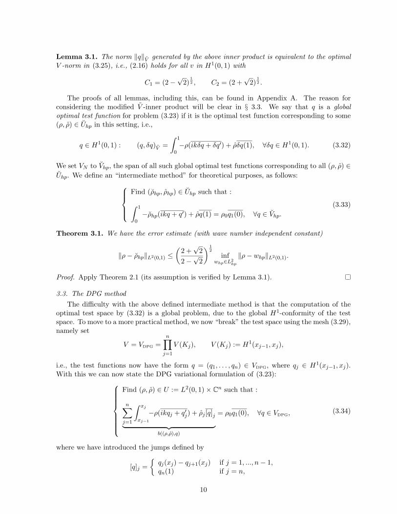
Lowering the degree of enrichment ∆p results in a gradual degradation in performance untilthe dimensions of the trial and enriched space are equal (Fig. 2). Higher enrichment obviouslyachieves better approximation of the optimal test functions, at the cost of more computationaleffort - we utilize a standard Cholesky factorization routine to solve the local system of equations,so the effort scales roughly as (p+∆p)3. However, we emphasize that this is a local, element-by-element operation, and therefore the resources required for computation of optimal test functionsare expected to be negligible compared to the cost of solving the final, global system. Moreover,

12

0.0 0.2 0.4 0.6 0.8 1.0x

1.0

0.5

0.0

0.5

1.0

ρ(x

)

kh=2.0π, p = 4, test p = 10, energy error = 0.068754

exactL2 projection, L2 error = 0.06875DPG, L2 error = 0.06875

0.0 0.2 0.4 0.6 0.8 1.0x

1.5

1.0

0.5

0.0

0.5

1.0

1.5

ρ(x

)

kh=16.0π, p = 28, test p = 34, energy error = 0.039817

exactL2 projection, L2 error = 0.04015DPG, L2 error = 0.04015

Figure 1: Comparison of the exact solution to the model problem (3.23) with the DPG solutionand the best L2 approximation, at two different wavenumbers (k = 2π and 16π, respectively).Both real and imaginary components of the solution ρ are shown. Discretizations employed inboth examples consist of one high-order element. Optimal test functions are computed corre-sponding to the optimal test space inner product (3.26), with degree of enrichment ∆p = 6. Inboth examples, the DPG solution coincides with the best approximation.

13

1 2 3 4 5 6 7∆p

0.00

0.01

0.02

0.03

0.04

0.05

0.06

DPG

sol

utio

n er

ror

kh=32π, p = 54

energy errorL2 errorbest approximation L2 error

Figure 2: Here we show the effect of the degree of enrichment ∆p on the error of the solutionby fixing the wavenumber k and discrete trial space, and solving the problem with varying ∆p.The optimal test functions are computed using the optimal test inner product (3.26). Moreenrichment provides better approximations to the true optimal test functions, resulting in lessL2 error. The reported energy error is computed by solving a discrete version of (2.14) over theenriched test space. Higher enrichment also brings this estimate closer to the true energy errordefined by (2.15).

14

in many applications we are likely to encounter redundant local problems (e.g. a patch ofuniform elements with identical material parameters), so optimal test functions computed onone element may be cached and re-used.

For the DPG setting, we employ the localizable inner product (3.36). In Figure 3, weplot solutions obtained with four linear elements per wavelength, for k corresponding to oneand 16 wavelengths over the length of the domain, respectively. We observe very good L2

stability, as indicated by the ratio of the DPG error to the best approximation error, regardlessof wavenumber, as illustrated in Fig. 4.

4. The Helmholtz model problem

In this section, we study the coupled Helmholtz problem in 1D, represented in terms ofpressure p and velocity u, coupled in a system of first-order differential equations. Again, wedemonstrate that with a proper choice of the norm for the test functions, the stability propertiesturn out to be wavenumber-independent. We start by analyzing the spectral problem and weprove robustness of the method in this simple setting. Then we introduce the DPG formulationthat delivers the same FE solution as the spectral one, when using the same trial FE basis.Hence, the robustness result will apply to the DPG solution as well.

4.1. The variational equationsWe consider the Helmholtz equation written as a system of two first order equations. The

new unknowns have physical meaning, e.g., in the theory of acoustical disturbances [8]. Givenan inflow data u0 ∈ C, the speed of sound c, and the density of the fluid ρ, we consider theboundary value problem

ikp

cρ+ u′ = 0 in Ω = (0, 1),

ik cρ u+ p′ = 0 in Ω = (0, 1),u(0) = u0 andp(1) = Zu(1),

(4.40)

where Z is an impedance parameter relating p and u at the right side boundary. The choiceZ = cρ leads to the exact right-traveling wave solution

u(x) = u0e−ikx, p(x) = cρu(x).

For the sake of simplicity, we will just consider the values Z = cρ = 1. Note that we use thenotation p for both polynomial degree and pressure. Which is meant is amply evident from thecontext, so no confusion will arise.

In the context of an unbroken test space, the natural variational formulation associated with(4.40) is

Find (p, u, p0, u1) ∈ U := [L2(Ω)]2 × C2, such that :

ik

∫Ωpq −

∫Ωuq′ + u1q(1) = u0q(0),

ik

∫Ωuv −

∫Ωpv′ + u1v(1)− p0v(0) = 0, ∀(q, v) ∈ V := [H1(Ω)]2.

(4.41)

15

0.0 0.2 0.4 0.6 0.8 1.0x

1.5

1.0

0.5

0.0

0.5

1.0

1.5

ρ(x

)

kh=0.5π, p = 1, test p = 7, energy error = 0.065227

exactL2 projection, L2 error = 0.088767DPG, L2 error = 0.088774

0.0 0.2 0.4 0.6 0.8 1.0x

1.5

1.0

0.5

0.0

0.5

1.0

1.5

ρ(x

)

kh=0.5π, p = 1, test p = 7, energy error = 0.065301

exactL2 projection, L2 error = 0.088767DPG, L2 error = 0.088767

Figure 3: Comparison of the exact solution to the model problem (3.23) with the DPG solutionand the best L2 approximation, at two different wavenumbers (k = 2π and 32π, respectively).Both real and imaginary components of the solution ρ are shown. Discretizations employedin both examples consist of four linear elements per wavelength. Optimal test functions arecomputed corresponding to the localizable inner product (3.31), with degree of enrichment ∆p =6. In both examples, the DPG solution nearly coincides with the best approximation, even whenk is increased several times in the bottom example.

16

100 101 102 103

k

1.00000

1.00005

1.00010

1.00015

||p−ph|| L

2

inf qh||p−q h|| L

2

Four linear elements per wavelength

Figure 4: As indicated by Theorem 3.2, the DPG method employing the localizable inner product(3.31) is robust with respect to wavenumber k. Here we take discretizations of four linearelements per wavelength and plot the ratio of the DPG error to the best approximation error asthe wavenumber is increased, observing that the ratio approaches a wavenumber-independentvalue (which is also very close to one).

17

As in § 3.1, this will immediately lead to a spectral method, once we select the trial space normin which we would like convergence, i.e.,

‖p, u, p0, u1‖2U := ‖p‖2L2 + ‖u‖2L2 + |p0|2 + |u1|2.

Then, the sesquilinear form on the left side of (4.41) yields the following optimal inner productand norm on V :(

(q, v), (δq, δv))V

=(ikq + v′, ikδq + δv′

)L2 +

(ikv + q′, ikδv + δq′

)L2

+(q(1) + v(1)

)(δq(1) + δv(1)

)+ v(0)δv(0)

‖q, v‖2V = ‖ikq + v′‖2L2 + ‖ikv + q′‖2L2 +∣∣q(1) + v(1)

∣∣2 + |v(0)|2.

(4.42)

Inspired by what we have observed in the previous section, we replace (4.42) with the followinglocalizable norm (and associated inner product):

‖q, v‖2V

= ‖ikq + v′‖2L2 + ‖ikv + q′‖2L2 + 1α‖v + q‖2L2 + 1

α‖v cos(kx) + iq sin(kx)‖2L2((q, v), (δq, δv)

)V

= (ikv + q′, ikδv + δq′)L2 + (ikq + v′, ikδq + δv′)L2 + 1α(v + q, δv + δq)L2

+ 1α

(v cos(kx) + iq sin(kx), δv cos(kx) + iδq sin(kx)

)L2 ,

(4.43)where α = 5+

√5

2 . Then we have the norm equivalence result (2.16), as stated in the next lemma.Its proof is in A.

Lemma 4.1. For all (q, v) in V ,

C1‖q, v‖2V ≤ ‖q, v‖2V ≤ C2‖q, v‖2V ,

with constants C1 = 5+√

52 − (5 + 2

√5)

12 and C2 = 5+

√5

2 + (5 + 2√

5)12 .

The next step is to consider an “intermediate method” as in § 3.2. Again let (3.29) define themesh of (0, 1). The trial space in this case is Uhp = [L2

hp(Ω)]2×C2. Let (pl, ul, p0l, u1l)l=1,...,N ⊂[L2(Ω)]2 × C2 be a finite trial basis such that each pl and ul are in L2

hp and are supported ona single element. With these as the trial functions and (4.43) as the inner product, we find thecorresponding optimal test functions. These are the global optimal test functions for this caseand we denote their span by Vhp. Let Uhp = (php, uhp, php, uhp) be the discrete solution fromthis method. Then we have the following robust error estimate for the intermediate problem.

Theorem 4.1. Let U = (p, u, p, u) be the exact solution of problem (4.41). Then

‖U− Uhp‖U ≤

√5 +√

52

+

√3 +√

52

infWhp∈Uhp

‖U−Whp‖U . (4.44)

Proof. This follows from Theorem 2.1 and Lemma 4.1.

As before, the global optimal test functions are expensive to compute. Hence we formulatethe DPG method with local optimal test functions next.

18

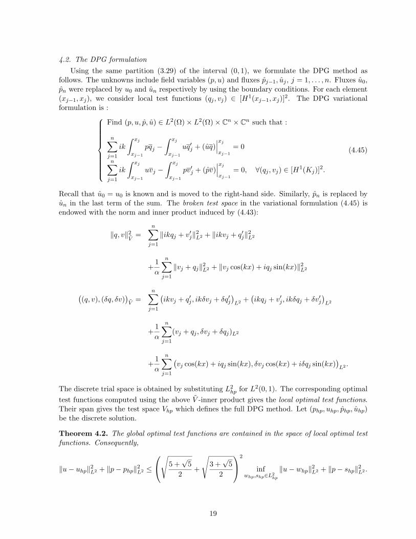
4.2. The DPG formulationUsing the same partition (3.29) of the interval (0, 1), we formulate the DPG method as

follows. The unknowns include field variables (p, u) and fluxes pj−1, uj , j = 1, . . . , n. Fluxes u0,pn were replaced by u0 and un respectively by using the boundary conditions. For each element(xj−1, xj), we consider local test functions (qj , vj) ∈ [H1(xj−1, xj)]2. The DPG variationalformulation is :

Find (p, u, p, u) ∈ L2(Ω)× L2(Ω)× Cn × Cn such that :

n∑j=1

ik

∫ xj

xj−1

pqj −∫ xj

xj−1

uq′j + (uq)∣∣∣xj

xj−1

= 0

n∑j=1

ik

∫ xj

xj−1

uvj −∫ xj

xj−1

pv′j + (pv)∣∣∣xj

xj−1

= 0, ∀(qj , vj) ∈ [H1(Kj)]2.

(4.45)

Recall that u0 = u0 is known and is moved to the right-hand side. Similarly, pn is replaced byun in the last term of the sum. The broken test space in the variational formulation (4.45) isendowed with the norm and inner product induced by (4.43):

‖q, v‖2V

=n∑j=1

‖ikqj + v′j‖2L2 + ‖ikvj + q′j‖2L2

+1α

n∑j=1

‖vj + qj‖2L2 + ‖vj cos(kx) + iqj sin(kx)‖2L2

((q, v), (δq, δv)

)V

=n∑j=1

(ikvj + q′j , ikδvj + δq′j

)L2 +

(ikqj + v′j , ikδqj + δv′j

)L2

+1α

n∑j=1

(vj + qj , δvj + δqj)L2

+1α

n∑j=1

(vj cos(kx) + iqj sin(kx), δvj cos(kx) + iδqj sin(kx)

)L2 .

The discrete trial space is obtained by substituting L2hp for L2(0, 1). The corresponding optimal

test functions computed using the above V -inner product gives the local optimal test functions.Their span gives the test space Vhp which defines the full DPG method. Let (php, uhp, php, uhp)be the discrete solution.

Theorem 4.2. The global optimal test functions are contained in the space of local optimal testfunctions. Consequently,

‖u− uhp‖2L2 + ‖p− php‖2L2 ≤

√5 +√

52

+

√3 +√

52

2

infwhp,shp∈L2

hp

‖u− whp‖2L2 + ‖p− shp‖2L2 .

19

The proof of this theorem is similar to the proof of Theorem 3.2 (cf. proof of Lemma 3.2),so we omit it.

Based on the discussion made in Section 2.4, the robustness estimation (4.44) also appliesfor the FE solution of this formulation, under analog considerations of the discrete trial space,aside from the additional 2(n− 1) fluxes.

4.3. Numerical resultsFigure 5 depicts solutions obtained with the spectral method, taking u0 = 1, Z = 1. Again

we have taken ∆p = 6 in constructing the enriched test space, which achieves nearly perfect L2

stability. Only the pressures p are plotted; the error in the velocity u is practically identical.The optimal test functions (q, v) in the spectral case may be expressed as the solutions of

the problem: ikq + v′ = −p in (0, 1),ikv + q′ = −u in (0, 1),v(0) = −p0,q(1) + v(1) = u1.

The optimal test functions for a number of basis functions are illustrated in Figures 6a-6d. Theiroscillatory behavior corresponding to wavenumber k makes clear the necessity of using sufficientorder p+ ∆p within the enriched test space.

For the multi-element case, we employ the localizable norm (4.43). Corresponding optimaltest functions are shown in Figures 7a-7d. Solutions and corresponding errors obtained withthe localizable norm are shown in Fig. 8. Again, we observe excellent stability with the DPGmethod. In contrast to standard methods, there is no degradation in stability with increasingwavenumber; indeed, if we adhere to a “rule of thumb” of n elements per wavelength as we varyk, we observe that the stability constant converges to a k-independent value (Figures 9a-9b.) Forcomparison, we plot in Fig. 10 a standard H1-conforming, Bubnov-Galerkin approximation php,as well as an H1-conforming approximation pblended obtained using specialized quadrature ruleswhich reduce the phase lag (see [1]). While they are obtained using the same discretization, i.e.order and number of elements, we must note that they only require solution of the pressure fieldp, while the DPG method requires the introduction of additional variables u, p, and u, requiringsignificantly more degrees of freedom.

Even at extremely poor discretization (e.g. 2 linear elements per wavelength), the methodremains stable, delivering results very near the L2 projection (Fig. 11).

Figure 12 shows a solution obtained using a high-order (p = 4) DPG method.

4.4. Helmholtz with PML truncationFinally, we consider the Helmholtz problem with PML truncation at the right end of the

domain, admitting only outgoing and evanescent waves. We employ the PML stretching function

z(x) =

x in (0, `)

x− iCk(x−`1−`

)4+ C

k

(x−`1−`

)4in (`, 1),

where ` is the position at which the PML begins, and C is a parameter controlling the strengthof the PML (we take C = 745 to achieve decay to near machine epsilon (double precision) for a

20

0.0 0.2 0.4 0.6 0.8 1.0x

1.0

0.5

0.0

0.5

1.0

p(x

)

kh=2.0π, p = 4, test p = 10, energy error = 0.09723

exactL2 projection, L2 error = 0.06875DPG, L2 error = 0.06875

0.0 0.2 0.4 0.6 0.8 1.0x

1.5

1.0

0.5

0.0

0.5

1.0

1.5

p(x

)

kh=16.0π, p = 27, test p = 33, energy error = 0.10292

exactL2 projection, L2 error = 0.07377DPG, L2 error = 0.07377

Figure 5: Comparison of the exact solution to the Helmholtz model problem (4.40) with thespectral method solution and the best L2 approximation, at two different wavenumbers (k = 2πand 16π, respectively). Both real and imaginary components of the pressure p are shown.Discretizations employed in both examples consist of one high-order element. Optimal testfunctions are computed corresponding to the optimal test space inner product (4.42), withdegree of enrichment ∆p = 6. In both examples, the spectral method solution coincides withthe best approximation.

21

0.0 0.2 0.4 0.6 0.8 1.01.0

0.5

0.0

0.5

1.0Test functions for p(0) =1, k=12.5663706144

qq (imag)vv (imag)

(a) Optimal test function for basis flux p0 = 1

0.0 0.2 0.4 0.6 0.8 1.01.0

0.5

0.0

0.5

1.0Test functions for u(1) =1, k=12.5663706144

qq (imag)vv (imag)

(b) Optimal test function for basis flux u1 = 1

Figure 6: Plots of the optimal test functions (q, v) for the Helmholtz spectral method, for k = 4π.The functions are defined using the optimal test inner product (4.42).

22

0.0 0.2 0.4 0.6 0.8 1.00.20

0.15

0.10

0.05

0.00

0.05

0.10Test functions for p(x) =1, k=12.5663706144

qq (imag)vv (imag)

(c) Optimal test function for basis function p(x) = 1

0.0 0.2 0.4 0.6 0.8 1.00.20

0.15

0.10

0.05

0.00

0.05

0.10Test functions for u(x) =1, k=12.5663706144

qq (imag)vv (imag)

(d) Optimal test function for basis function u(x) = 1

Figure 6: (continued) Plots of the optimal test functions (q, v) for the Helmholtz spectral method,for k = 4π. The functions are defined using the optimal test inner product (4.42).

23

0.0 0.2 0.4 0.6 0.8 1.04

3

2

1

0

1

2

3

4Test functions for p(0) =1, k=12.5663706144

qq (imag)vv (imag)

(a) Optimal test function for basis flux p0 = 1

0.0 0.2 0.4 0.6 0.8 1.04

3

2

1

0

1

2

3

4Test functions for u(1) =1, k=12.5663706144

qq (imag)vv (imag)

(b) Optimal test function for basis flux u1 = 1

Figure 7: Plots of the optimal test functions (q, v) for the Helmholtz spectral method, for k = 4π.The functions are defined using the localizable inner product (4.43).

24

0.0 0.2 0.4 0.6 0.80.08

0.06

0.04

0.02

0.00

Test functions for p(x) =1, k=12.5663706144

qq (imag)vv (imag)

(c) Optimal test function for basis function p(x) = 1

0.0 0.2 0.4 0.6 0.8

0.08

0.06

0.04

0.02

0.00

Test functions for u(x) =1, k=12.5663706144

qq (imag)vv (imag)

(d) Optimal test function for basis function u(x) = 1

Figure 7: (continued) Plots of the optimal test functions (q, v) for the Helmholtz spectral method,for k = 4π. The functions are defined using the localizable inner product (4.43).

25

0.0 0.2 0.4 0.6 0.8 1.0x

1.5

1.0

0.5

0.0

0.5

1.0

1.5

p(x

)

kh=0.5π, p = 1, test p = 7, energy error = 0.1254

exactL2 projection, L2 error = 0.08877DPG, L2 error = 0.08881

0.0 0.2 0.4 0.6 0.8 1.0x

1.5

1.0

0.5

0.0

0.5

1.0

1.5

p(x

)

kh=0.5π, p = 1, test p = 7, energy error = 0.12554

exactL2 projection, L2 error = 0.08877DPG, L2 error = 0.08882

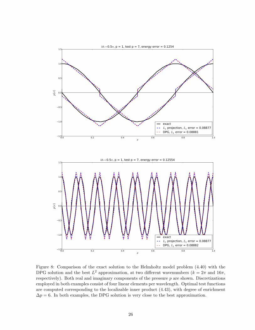
Figure 8: Comparison of the exact solution to the Helmholtz model problem (4.40) with theDPG solution and the best L2 approximation, at two different wavenumbers (k = 2π and 16π,respectively). Both real and imaginary components of the pressure p are shown. Discretizationsemployed in both examples consist of four linear elements per wavelength. Optimal test functionsare computed corresponding to the localizable inner product (4.43), with degree of enrichment∆p = 6. In both examples, the DPG solution is very close to the best approximation.

26

100 101 102 103 104

k

1.00052

1.00053

1.00054

1.00055

1.00056

1.00057

1.00058

1.00059

1.00060

√ ||p−ph||2 L

2+||u−uh||2 L

2

inf vh,w

h

√ ||p−v h||2 L

2+||u−wh||2 L

2

Four linear elements per wavelength

(a) Four linear elements per wavelength

100 101 102 103 104

k

1.00010

1.00015

1.00020

1.00025

1.00030

1.00035

1.00040

1.00045

1.00050

√ ||p−ph||2 L

2+||u−uh||2 L

2

inf vh,w

h

√ ||p−v h||2 L

2+||u−wh||2 L

2

One p=4 element per wavelength

(b) One p = 4 element per wavelength

Figure 9: As indicated by Theorem 4.2, the DPG method employing the localizable innerproduct (4.43) is robust with respect to wavenumber k. Here we take discretizations of fourlinear elements per wavelength (top) and one p = 4 element per wavelength (bottom) and plotthe ratio of the DPG error to the best approximation error as the wavenumber is increased,observing that the ratio approaches a wavenumber-independent value (which is also very closeto one).

27

0.70 0.75 0.80 0.85 0.90 0.95 1.00x

1.5

1.0

0.5

0.0

0.5

1.0

p(x

)

kh=π/3, p = 1, test p = 7, energy error = 0.05689

exactstandard H1 -conforming, L2 error = 1.19609H1 -conforming w/ special quadrature, L2 error = 0.13379DPG, L2 error = 0.04024

Figure 10: Comparison of the exact solution to the Helmholtz model problem (4.40) with theDPG solution, a standard H1-conforming FEM solution, and another H1-conforming methodemploying specialized quadrature rules which reduce phase error. Both real and imaginary partsof the pressure p are shown. Six linear elements per wavelength are used with each method.Optimal test functions for the DPG method are computed corresponding to the localizable innerproduct (4.43), with degree of enrichment ∆p = 6.

28

0.0 0.2 0.4 0.6 0.8x

1.5

1.0

0.5

0.0

0.5

1.0

p(x

)

kh=1.0π, p = 1, test p = 7, energy error = 0.44632

exactL2 projection, L2 error = 0.31929DPG, L2 error = 0.32015

Figure 11: Comparison of the exact solution to the Helmholtz model problem (4.40) with theDPG solution and the best L2 approximation. Both real and imaginary components of thepressure p are shown. In this example, we take a rather coarse discretization of two linearelements per wavelength, but still obtain results very near the L2 best approximation. Optimaltest functions are computed corresponding to the localizable inner product (4.43), with degreeof enrichment ∆p = 6.

29

0.0 0.2 0.4 0.6 0.8 1.0x

1.0

0.5

0.0

0.5

1.0

p(x

)

kh=2.0π, p = 4, test p = 10, energy error = 0.09717

exactL2 projection, L2 error = 0.06875DPG, L2 error = 0.06876

Figure 12: Comparison of the exact solution to the Helmholtz model problem (4.40) with theDPG solution and the best L2 approximation, at k = 16π. Both real and imaginary componentsof the pressure p are shown. The trial space discretization consists of one p = 4 element perwavelength. Optimal test functions are computed corresponding to the localizable inner product(4.43), with degree of enrichment ∆p = 6.

30

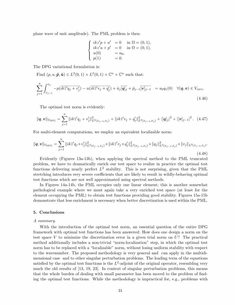
plane wave of unit amplitude). The PML problem is then:ikz′p+ u′ = 0 in Ω = (0, 1),ikz′u+ p′ = 0 in Ω = (0, 1),u(0) = u0,p(1) = 0.

The DPG variational formulation is:

Find (p, u, p, u) ∈ L2(0, 1)× L2(0, 1)× Cn × Cn such that:

n∑j=1

∫ xj

xj−1

−p(ikz′qj + v′j)− u(ikz′vj + q′j) + uj [q]j + pj−1[v]j−1 = u0q1(0) ∀(q,v) ∈ VDPG.

(4.46)

The optimal test norm is evidently:

‖q,v‖VDPG=

n∑j=1

‖ikz′qj + v′j‖2L2(xj−1,xj) + ‖ikz′vj + q′j‖2L2(xj−1,xj) + |[q]j |2 + |[v]j−1|2 . (4.47)

For multi-element computations, we employ an equivalent localizable norm:

‖q,v‖VDPG=

n∑j=1

‖ikz′qj+v′j‖2L2(xj−1,xj)+‖ikz′vj+q′j‖2L2(xj−1,xj)+‖qj‖

2L2(xj−1,xj)+‖vj‖L2(xj−1,xj).

(4.48)Evidently (Figures 13a-13b), when applying the spectral method to the PML truncated

problem, we have to dramatically enrich our test space to realize in practice the optimal testfunctions delivering nearly perfect L2 stability. This is not surprising, given that the PMLstretching introduces very severe coefficients that are likely to result in wildly-behaving optimaltest functions which are not well approximated using spectral methods.

In Figures 14a-14b, the PML occupies only one linear element; this is another somewhatpathological example where we must again take a very enriched test space (at least for theelement occupying the PML) to obtain test functions providing good stability. Figures 15a-15bdemonstrate that less enrichment is necessary when better discretization is used within the PML.

5. Conclusions

A summary.With the introduction of the optimal test norm, an essential question of the entire DPG

framework with optimal test functions has been answered: How does one design a norm on thetest space V to minimize the discretization error in a given trial norm on U? The practicalmethod additionally includes a non-trivial “norm-localization” step, in which the optimal testnorm has to be replaced with a “localizable” norm, without losing uniform stability with respectto the wavenumber. The proposed methodology is very general and can apply in the multidi-mensional case and to other singular perturbation problems. The leading term of the equationssatisfied by the optimal test functions is the L2-adjoint of the original operator, resembling verymuch the old results of [13, 19, 23]. In context of singular perturbation problems, this meansthat the whole burden of dealing with small parameter has been moved to the problem of find-ing the optimal test functions. While the methodology is impractical for, e.g., problems with

31

0.0 0.2 0.4 0.6 0.8 1.0x

1.5

1.0

0.5

0.0

0.5

1.0

1.5

p(x

)

PML

kh=4.0π, p = 9, test p = 15

exactL2 projection, L2 error = 0.17448DPG, L2 error = 0.32609

(a) Insufficiently enriched test space (∆p = 6)

0.0 0.2 0.4 0.6 0.8 1.0x

1.5

1.0

0.5

0.0

0.5

1.0

1.5

p(x

)

PML

kh=4.0π, p = 9, test p = 69

exactL2 projection, L2 error = 0.17448DPG, L2 error = 0.17462

(b) Dramatically enriched test space (∆p = 60)

Figure 13: Comparison of the exact solution to the PML truncated Helmholtz problem (4.46)with the spectral method solution and the best L2 approximation, at k = 4π. The PMLtruncation begins at x = 0.5. Both real and imaginary components of the pressure p are shown.One p = 9 element is employed. Optimal test functions are computed corresponding to theoptimal norm (4.47); high degree of enrichment is necessary in order to approximate the trueoptimal test functions in this example.

32

0.0 0.2 0.4 0.6 0.8 1.0x

1.5

1.0

0.5

0.0

0.5

1.0

1.5

p(x

)

PML

kh=0.5π, p = 1, test p = 7

exactL2 projection, L2 error = 0.12606DPG, L2 error = 0.50283

(a) Insufficiently enriched test space (∆p = 6)

0.0 0.2 0.4 0.6 0.8 1.0x

1.5

1.0

0.5

0.0

0.5

1.0

1.5

p(x

)

PML

kh=0.5π, p = 1, test p = 41

exactL2 projection, L2 error = 0.12606DPG, L2 error = 0.12779

(b) Dramatically enriched test space (∆p = 40)

Figure 14: Comparison of the exact solution to the PML truncated Helmholtz problem (4.46)with the DPG solution and the best L2 approximation. Both real and imaginary components ofthe pressure p are shown. Four linear elements per wavelength are used, and the PML occupiesthe last element. Optimal test functions are computed corresponding to the localizable norm(4.48); high degree of enrichment is necessary in order to approximate the true optimal testfunctions with support within the PML.

33

0.0 0.2 0.4 0.6 0.8 1.0x

1.5

1.0

0.5

0.0

0.5

1.0

1.5

p(x

)

PML

kh=0.5π, p = 1, test p = 7

exactL2 projection, L2 error = 0.08928DPG, L2 error = 0.0901

(a)

0.75 0.80 0.85 0.90 0.95 1.00x

1.0

0.5

0.0

0.5

1.0

p(x

)

PML

kh=0.5π, p = 1, test p = 7

exactL2 projection, L2 error = 0.08928DPG, L2 error = 0.0901

(b) Zoom of Fig. 15a near the PML

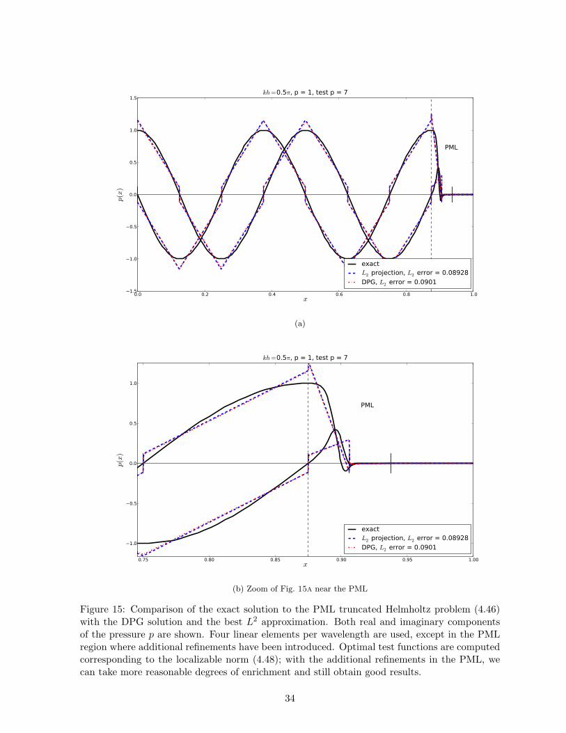
Figure 15: Comparison of the exact solution to the PML truncated Helmholtz problem (4.46)with the DPG solution and the best L2 approximation. Both real and imaginary componentsof the pressure p are shown. Four linear elements per wavelength are used, except in the PMLregion where additional refinements have been introduced. Optimal test functions are computedcorresponding to the localizable norm (4.48); with the additional refinements in the PML, wecan take more reasonable degrees of enrichment and still obtain good results.

34

boundary layers (solving the adjoint equation on a large element is as difficult as solving theoriginal problem), it seems to be perfectly suited for wave propagation where the element size isdetermined by the need to resolve the wave structure (control of the best approximation error).

Performance vs. traditional methodsWhile extremely stable in contrast to traditional Bubnov-Galerkin approximations for the

Helmholtz problem, DPG forces us to consider the mixed problem in which we compute pressure,velocity, and additional fluxes. For a discretization of n elements of order p per wavelength,for a domain of m wavelengths, the DPG formulation requires 2(p + 1)mn + 2mn degrees offreedom, while a standard H1 conforming formulation involving only pressure requires pmn.After performing static condensation on the interior degrees of freedom, we are left with asystem of dimension 2mn for DPG versus mn for the H1 conforming method. This implies thatthe DPG method will be competitive when compared with standard finite elements only forlarge wavenumbers. Here we also remark that while static condensation for the H1 conformingmethod requires us to avoid element sizes h ≈ jπ

k , j ∈ N, in order to avoid the associated interiormodes at the given wavenumber, in the mixed formulation which involves both p and u, thereis no such trouble – the problem

ikp+ u′ = 0,iku+ p′ = 0,

u(xi−1) = u(xi) = p(xi−1) = p(xi) = 0

admits only the trivial solution. Hence, our element interior submatrices can always be factoredwithout any concern of encountering interior modes, which should make static condensation,nested dissection, and other domain decomposition approaches robust.

Current and future workThe presented analysis and experiments are being extended to the two dimensional (2D)

problem. Preliminary numerical results indicate that the presented methodology extends tomultiple dimensions, with either zero, or numerically unobservable, phase error. A 2D version ofthe method on a structured rectangular mesh does not fit within the class of generalized finiteelement methods (GFEM) analyzed in [4]. Our current efforts concentrate on a 2D convergenceanalysis.

DPG methods can prove to be an attractive choice for high-frequency wave-propagationproblems. Our methodology also offers the possibility of using plane waves or other waves (see,e.g. [15, 22]) for trial functions, with the hope of improving the approximation properties ofthe underlying space for a given problem. The theory of optimal test functions and optimaltest norm continues to apply with better trial space choices. We emphasize nonetheless thatthe control of phase error is related to stability and not approximability, and the stability iscontrolled by the choice of test functions.

A. Proofs of the lemmas

Proof of Lemma 3.1. We need to prove that ‖q‖2V

= ‖ikq + q′‖2L2(0,1) + 12‖q‖

2L2(0,1) and ‖q‖2V =

‖ikq + q′‖2L2(0,1) + |q(1)|2 define equivalent norms on H1(0, 1). Let q = eikxq. Since k is real,

‖q′‖2L2 = ‖ikq + q′‖2L2 , ‖q‖2L2 = ‖q‖2L2 and |q(1)|2 = |q(1)|2.

35

Thus, we only need to bound ‖q′‖2L2 + |q(1)|2 above and below by ‖q′‖2L2 + 12‖q‖

2L2 . We use the

Fundamental Theorem of Calculus q(1)− q(x) =∫ 1x q(s) ds, together with standard techniques

involving Young’s inequality to estimate |q(1)|2 and ‖q‖2L2 . For every ε > 0 and δ > 0,

|q(1)|2 ≤ (1 + ε)‖q‖2L2 + 1+εε ‖q

′‖2L2 ,

‖q‖2L2 ≤ (1 + δ)|q(1)|2 + 1+δδ ‖q

′‖2L2 .

Thus we already see that the norms ‖q‖V and ‖q‖V are equivalent with constants of equivalenceindependent of k.

The rest of the proof is devoted to finding the constants stated in the lemma. To obtain thebest constants, we first note that the above implies

‖q‖2V ≤(1 + ε−1(1 + ε)

)‖q′‖2L2 + (1 + ε)‖q‖2L2 (A.49)

≤ F1(ε, δ)‖q′‖2L2 + F2(ε, δ)|q(1)|2, (A.50)

where F1(ε, δ) =(1 + 1+ε

ε + (1 + ε)1+δδ

)and F2(ε, δ) = (1+ε)(1+δ). Then we minimize F2(ε, δ)

subject to the constraints ε > 0, δ > 0, and F2(ε, δ) = F1(ε, δ), to obtain ε =√

22 and δ = 1+

√2.

With these values, we have

‖q‖2V ≤(2 +√

2)(‖q′‖2L2 +

12‖q‖2L2

), by (A.49),(

2 +√

2)(‖q′‖2L2 +

12‖q‖2L2

)≤(2 +√

2)(2 +

√2

2)(‖q′‖2L2 + |q(1)|2

), by (A.50).

These two inequalities prove the lemma.

Proof of Lemma 3.2. Let us prove that Vhp ⊆ Vhp. Clearly this will imply that ρhp = ρhp dueto unique solvability.

Let q ∈ Vhp denote the global optimal test function corresponding to (ρ, ρ) ∈ Uhp. Itsolves (3.32), i.e.,∫ 1

0(ikq + q′)(ikδq + δq′) +

12

∫ 1

0qδq =

∫ 1

0−ρ(ikδq + δq′) + ρδq(1),

for all δq ∈ H1(0, 1). As ρ is smooth (a polynomial) within each element Kj , this variationalequation translates into the following differential, boundary and interface equations:

−q′′ − 2ikq′ + (k2 +12

)q = ρ′ + ikρ in (xj−1, xj) for j = 1, . . . , n

[ikq + q′ + ρ]j = 0 for j = 1, . . . , n− 1

(ikq + q′ + ρ)(1) = ρ

−(ikq + q′ + ρ)(0) = 0.

(A.51)

where, as before, the [ · ]j denotes the jump of the argument at xj .Now, let δqj ∈ H1(Kj). Multiplying (A.51)1 by δqj , integrating over each element, and

summing up over all elements, we get

n∑j=1

−∫ xj

xj−1

(ikq + q′ + ρ)′δqj −∫ xj

xj−1

(ik(q′ + ρ)− (k2 +

12

)q)δqj

= 0.

36

Integrating the first term by parts, using the continuity of ikq+ q′+ρ at element interfaces, andusing the boundary conditions in (A.51)3,4, we obtain

n∑j=1

(ikq + q′, ikδqj + δq′j

)L2(Kj)

+12

(q, δqj)L2(Kj)

= ρδqn(1)−n∑j=1

∫ xj

xj−1

ρ(ikqj + q′j) +n−1∑j=1

(ikq + q′ + ρ)(xj)[δq]j .

The left hand side equals (q, δq)V , the inner product in (3.36) for the multielement case. Theright hand side is the sesquilinear form of the DPG formulation (3.37) with

ρhp = ρ,

ρhpj = (ikq + q′ + ρ)(xj), for j = 1, ..., n− 1,

ρhpn = ρ.

Therefore, the global optimal test function q is a linear combination of the local optimal testfunctions associated with ρ, (ikq + q′ + ρ)(xj) and ρ.

Proof of Lemma 4.1. Let r = v+q2 and s = v−q

2 . Using the same idea as in the proof ofLemma 3.1, we set r = eikxr and s = e−ikxs, so

e−ikxr′ = ikr + r′ and eikxs′ = −iks+ s′.

The norm ‖q, v‖2V can be expressed in terms of these new functions as

‖q, v‖2V = ‖ik(r − s) + (r + s)′‖2L2 + ‖ik(r + s) + (r − s)′‖2L2 +∣∣2r(1)

∣∣2 + |(r + s)(0)|2

=∥∥e−ikxr′ + eikxs′

∥∥2

L2 +∥∥e−ikxr′ − eikxs′∥∥2

L2 +∣∣2r(1)

∣∣2 + |(r + s)(0)|2

= 2‖r′‖2L2 + 2‖s′‖2L2 +∣∣2r(1)

∣∣2 + |(r + s)(0)|2.

On one hand we have

|2r(1)|2 ≤ (1 + ε1)‖2r‖2L2 + 4(

1+ε1ε1

)‖r′‖2L2

|(r + s)(0)|2 ≤ (1 + ε2)‖r + s‖2L2 + 1+ε2ε2‖r′ + s′‖2L2

≤ (1 + ε2)‖r + s‖2L2 + 1+ε2ε2

((1 + ε3)‖r′‖2L2 + 1+ε3

ε3‖s′‖2L2

).

Observe that ‖2r‖2L2 = ‖v + q‖2L2 and ‖r + s‖2L2 = ‖v cos(kx) + iq sin(kx)‖2L2 .On the other hand, we have

‖2r‖2L2 ≤ (1 + δ1)|2r(1)|2 + 4(

1+δ1δ1

)‖r′‖2L2

‖r + s‖2L2 ≤ (1 + δ2)|(r + s)(0)|2 + 1+δ2ε2‖r′ + s′‖2L2

≤ (1 + δ2)|(r + s)(0)|2 + 1+δ2δ2

((1 + δ3)‖r′‖2L2 + 1+δ3

ε3‖s′‖2L2

).

37

We choose ε1 = ε2, δ1 = δ2 and ε3 = δ3 =√

5− 2. As a consequence,

‖q, v‖2V ≤ (1 + f1(ε1))(

2‖r′‖2L2 + 2‖s′‖2L2

)+ f2(ε1)

(‖2r‖2L2 + ‖r + s‖2L2

)≤ (1 + f1(ε1) + f2(ε1)f1(δ1))

(2‖r′‖2L2 + 2‖s′‖2L2

)+f2(ε1)f2(δ1)

(|2r(1)|2 + |(r + s)(0)|2

),

(A.52)

where the functions of f1 and f2 are defined by :

f1(x) = C

(1 + x

x

), f2(x) = (1 + x) and C =

√5 + 32

.

We arrive at the minimization problem :min f2(ε1)f2(δ1)

ε1 > 0δ1 > 0

1 + f1(ε1) + f2(ε1)f1(δ1)− f2(ε1)f2(δ1) = 0,

whose solutions are ε1 =√

CC+1 and δ1 = f1(ε1). Replacing these values on the inequality (A.52)

we obtain :‖q, v‖2V ≤

√C + 1

(√C +

√C + 1

)(2‖r′‖2L2 + 2‖s′‖2L2 + 1

C+1

(‖2r‖2L2 + ‖r + s‖2L2

))≤√C + 1

(√C +

√C + 1

)(1 +

√CC+1

)‖q, v‖2V .

Hence,

C1 =(

1 +√

CC+1

)−1=√C + 1

(√C + 1−

√C)

= 5+√

52 − (5 + 2

√5)

12 ,

C2 =√C + 1

(√C + 1 +

√C)

= 5+√

52 + (5 + 2

√5)

12 .

Acknowledgements

J. Zitelli was supported by an ONR Graduate Traineeship and CAM Fellowhip. I. Muga wassupported by Sistema Bicentenario BECAS CHILE (Chilean Government). L. Demkowicz wassupported by a Collaborative Research Grant from King Abdullah University of Science andTechnology (KAUST). J. Gopalakrishnan was supported by the National Science Foundationunder grant DMS-1014817.

References

[1] M. Ainsworth and H. Wajid. Optimally blended spectral-finite element scheme for wavepropagation, and non-standard reduced integration. University of Strathclyde MathematicsResearch Report, 12, 2009.

38

[2] I. Babuska, F. Ihlenburg, E.T. Paik, and S.A. Sauter. A generalized finite element methodfor solving the Helmholtz equation in two dimensions with minimal pollution. Comput.Methods Appl. Mech. Engrg., 128:325–359, 1995.

[3] I. Babuska and J. M. Melenk. The partition of unity method. International Journal ofNumerical Methods in Engineering, 40:727–758, 1996.

[4] Ivo M. Babuska and Stefan A. Sauter. Is the pollution effect of the FEM avoidable for thehelmholtz equation considering high wave numbers? SIAM J. Numer. Anal., 34(6):2392–2423, 1997.

[5] P. E. Barbone and I. Harari. Nearly H1-optimal finite element methods. Comput. MethodsAppl. Mech. Engrg., 190:5679 – 5690, 2001.

[6] C.L. Bottasso, S. Micheletti, and R. Sacco. The discontinuous Petrov-Galerkin method forelliptic problems. Comput. Methods Appl. Mech. Engrg., 191:3391–3409, 2002.

[7] Z. Cai, R. Lazarov, T. A. Manteuffel, and S. F. McCormick. First-order system least squaresfor second-order partial differential equations. SIAM J. Numer. Anal., 31:1785 – 1799, 1994.

[8] R. Courant and K. O. Friedrichs. Supersonic Flow and Shock Waves. Interscience Publish-ers, Inc., New York, N.Y., 1948.

[9] L. Demkowicz. Babuska ⇔ Brezzi ? Technical report, ICES, 2006.

[10] L. Demkowicz and J. Gopalakrishnan. A class of discontinuous Petrov-Galerkin methods.Part I: The transport equation. Computer Methods in Applied Mechanics and Engineering,199 (2010), pp. 1558—1572.

[11] L. Demkowicz and J. Gopalakrishnan. A class of discontinuous Petrov-Galerkin methods.Part II: Optimal test functions. Technical Report 16, ICES, 2009. In print (Numer. MethodsPartial Differential Equations).

[12] L. Demkowicz, J. Gopalakrishnan, and A. Niemi. A class of discontinuous Petrov-Galerkinmethods. Part III: Adaptivity. Technical Report 1, ICES, 2010. In review.

[13] L. Demkowicz and J. T. Oden. An adaptive characteristic Petrov-Galerkin finite elementmethod for convection-dominated linear and nonlinear parabolic problems in one spacevariable. Journal of Computational Physics, 68(1):188–273, 1986.

[14] L. Demkowicz and J. T. Oden. An adaptive characteristic Petrov-Galerkin finite elementmethod for convection-dominated linear and nonlinear parabolic problems in two spacevariables. Comput. Methods Appl. Mech. Engrg., 55(1-2):65–87, 1986.

[15] C. Farhat, I. Harari, and L. P. Franca. The discontinuous enrichment method. ComputerMethods in Applied Mechanics and Engineering, 190(48):6455 – 6479, 2001.

[16] Charbel Farhat, Isaac Harari, and Ulrich Hetmaniuk. A discontinuous galerkin method withlagrange multipliers for the solution of helmholtz problems in the mid-frequency regime.Computer Methods in Applied Mechanics and Engineering, 192(11-12):1389 – 1419, 2003.

[17] X. Feng and H. Wu. Discontinuous Galerkin methods for the Helmholtz equation with largewave number. SIAM J. Numer. Anal., 47:2872 – 2896, 2009.

39

[18] Leopoldo P. Franca, Charbel Farhat, Antonini P. Macedo, and Michel Lesoinne. Residual-free bubbles for the Helmholtz equation. Internat. J. Numer. Methods Engrg., 40(21):4003–4009, 1997.

[19] Dan Givoli. Nonlocal and semilocal optimal weighting functions for symmetric problemsinvolving a small parameter. Internat. J. Numer. Methods Engrg., 26(6):1281–1298, 1988.

[20] Isaac Harari. A survey of finite element methods for time-harmonic acoustics. ComputerMethods in Applied Mechanics and Engineering, 195(13-16):1594 – 1607, 2006. A Tributeto Thomas J.R. Hughes on the Occasion of his 60th Birthday.

[21] Isaac Harari and Thomas J. R. Hughes. Finite element methods for the helmholtz equationin an exterior domain: Model problems. Computer Methods in Applied Mechanics andEngineering, 87(1):59 – 96, 1991.

[22] R. Hiptmair, A. Moiola, and I. Perugia. Plane wave discontinuous Galerkin methods forthe 2D Helmholtz equation: analysis of the p-version. Technical Report 20, Seminar forApplied Mathematics, ETH Zurich, 2009.

[23] T.J.R. Hughes and A. Brooks. A multidimensional upwind scheme with no crosswinddiffusion. In Finite Element Methods for Convection Dominated Flows (Papers, WinterAnn. Meeting Amer. Soc. Mech. Engrs., New York, 1979), volume 34 of AMD, pages 19–35, New York, 1979. Amer. Soc. Mech. Engrs. (ASME).

[24] F. Ihlenburg. Finite Element Analysis of Acoustic Scattering, volume 132 of Applied Math-ematical Sciences. Springer-Verlag, New York, 1998.

[25] A. F. D. Loula and D. T. Fernandes. A quasi optimal Petrov-Galerkin method for Helmholtzproblem. Internat. J. Numer. Methods Engrg., 80:1595 – 1622, 2009.

[26] Assad A. Oberai and Peter M. Pinsky. A numerical comparison of finite element methodsfor the Helmholtz equation. Journal of Computational Acoustics, 8(1):211, 2000.

[27] J.T. Oden and L.F. Demkowicz. Applied Functional Analysis for Science and Engineering.Chapman & Hall/CRC Press, Boca Raton, 2010. Second edition.

[28] Lonny L. Thompson. A review of finite-element methods for time-harmonic acoustics. TheJournal of the Acoustical Society of America, 119(3):1315–1330, 2006.

[29] Lonny L. Thompson and Peter M. Pinsky. A Galerkin least squares finite element methodfor the two-dimensional Helmholtz equation. International Journal for Numerical Methodsin Engineering, 38:371 – 397, 1995.

[30] K. Yosida. Functional Analysis. Springer-Verlag, Berlin, 1995. Reprint of the sixth (1980)edition.

40