A combinatorial framework for the design of (pseudoknotted) RNA algorithms Yann Ponty ? and Cédric Saule 1 LIX, École Polytechnique/CNRS/INRIA AMIB 2 LRI, Université Paris-Sud/XI/INRIA AMIB Abstract. We extend an hypergraph representation, introduced by Finkelstein and Roytberg, to unify dynamic programming algorithms in the context of RNA folding with pseudoknots. Classic applica- tions of RNA dynamic programming (Energy minimization, partition function, base-pair probabili- ties. . . ) are reformulated within this framework, giving rise to very simple algorithms. This reformu- lation allows one to conceptually detach the conformation space/energy model – captured by the hypergraph model – from the specific application, assuming unambiguity of the decomposition. To ensure the latter property, we propose a new combinatorial methodology based on generating func- tions. We extend the set of generic applications by proposing an exact algorithm for extracting gener- alized moments in weighted distribution, generalizing a prior contribution by Miklos and al. Finally, we illustrate our full-fledged programme on three exemplary conformation spaces (secondary struc- tures, Akutsu’s simple type pseudoknots and kissing hairpins). This readily gives sets of algorithms that are either novel or have complexity comparable to classic implementations for minimization and Boltzmann ensemble applications of dynamic programming. Key words: RNA folding, Pseudoknots, Boltzmann Ensemble, Hypergraphs, Dynamic Programming 1 Introduction Motivation. Over the past decades biology as a field has become increasingly aware of the importance and diversity of roles played by ribonucleic acids (RNA). In addition to playing house-keeping parts, as initially contemplated by the proteo-centric view of cellular processes, RNA is now accepted as a major player of gene regulation mechanisms. For instance silencing activity (miRNAs, siRNAs) or multi-stable cis-regulatory elements (riboswitches) are currently the subject of many research. Furthermore a recent genome-wide experiment has revealed that a large portion of the human genome was subject to tran- scription into RNA. While it is unlikely for all these transcripts to be functional as RNAs, novel classes and roles are currently suspected for novel RNAs. Most of the functional roles played by RNA require the RNA to adopt a specific structure to make an interaction possible, hide/exhibit an active site or allow for a catalytic action (Ribozymes). Being able to understand and simulate how RNA folds is therefore a crucial step toward understanding its function. Ab initio secondary structure prediction. Initial algorithmic methods for the ab initio prediction of RNA folding considered a coarse-grain conformation space, the secondary structure, where each conforma- tion is defined as a non-crossing subset of admissible base-pairs. The restriction of potential contacts allowed Nussinov and Jacobson (36) to design a Θ(n 3 ) dynamic-programming algorithm to maximize the number of base-pairs. Building on a nearest neighbor model for the free-energy proposed by Tinoco et al (48) and extended by the Turner group, Zuker and Stiegler (53) created MFOLD,a Θ(n 3 ) algorithm for minimizing the free-energy (MFE folding), later shown to predict correctly ∼73% of base-pairs on a benchmark of RNAs of length < 700 nucleotides (31). An independent implementation of the algo- rithm is proposed within the VIENNA package maintained by Hofacker (21). Probabilistic alternatives (SFOLD (10), CONTRAFOLD (13) and CENTROIDFOLD (19)) have also recently been proposed with sub- stantial success, relying on a dynamic programming scheme similar to that of MFOLD to traverse the ? To whom correspondence should be addressed
Transcript
A combinatorial framework for the design of (pseudoknotted) RNAalgorithms
Abstract. We extend an hypergraph representation, introduced by Finkelstein and Roytberg, to unifydynamic programming algorithms in the context of RNA folding with pseudoknots. Classic applica-tions of RNA dynamic programming (Energy minimization, partition function, base-pair probabili-ties. . . ) are reformulated within this framework, giving rise to very simple algorithms. This reformu-lation allows one to conceptually detach the conformation space/energy model – captured by thehypergraph model – from the specific application, assuming unambiguity of the decomposition. Toensure the latter property, we propose a new combinatorial methodology based on generating func-tions. We extend the set of generic applications by proposing an exact algorithm for extracting gener-alized moments in weighted distribution, generalizing a prior contribution by Miklos and al. Finally,we illustrate our full-fledged programme on three exemplary conformation spaces (secondary struc-tures, Akutsu’s simple type pseudoknots and kissing hairpins). This readily gives sets of algorithmsthat are either novel or have complexity comparable to classic implementations for minimizationand Boltzmann ensemble applications of dynamic programming.
Motivation. Over the past decades biology as a field has become increasingly aware of the importanceand diversity of roles played by ribonucleic acids (RNA). In addition to playing house-keeping parts, asinitially contemplated by the proteo-centric view of cellular processes, RNA is now accepted as a majorplayer of gene regulation mechanisms. For instance silencing activity (miRNAs, siRNAs) or multi-stablecis-regulatory elements (riboswitches) are currently the subject of many research. Furthermore a recentgenome-wide experiment has revealed that a large portion of the human genome was subject to tran-scription into RNA. While it is unlikely for all these transcripts to be functional as RNAs, novel classesand roles are currently suspected for novel RNAs. Most of the functional roles played by RNA require theRNA to adopt a specific structure to make an interaction possible, hide/exhibit an active site or allowfor a catalytic action (Ribozymes). Being able to understand and simulate how RNA folds is therefore acrucial step toward understanding its function.Ab initio secondary structure prediction. Initial algorithmic methods for the ab initio prediction of RNAfolding considered a coarse-grain conformation space, the secondary structure, where each conforma-tion is defined as a non-crossing subset of admissible base-pairs. The restriction of potential contactsallowed Nussinov and Jacobson (36) to design a Θ(n3) dynamic-programming algorithm to maximizethe number of base-pairs. Building on a nearest neighbor model for the free-energy proposed by Tinocoet al (48) and extended by the Turner group, Zuker and Stiegler (53) created MFOLD, a Θ(n3) algorithmfor minimizing the free-energy (MFE folding), later shown to predict correctly ∼73% of base-pairs ona benchmark of RNAs of length < 700 nucleotides (31). An independent implementation of the algo-rithm is proposed within the VIENNA package maintained by Hofacker (21). Probabilistic alternatives(SFOLD (10), CONTRAFOLD (13) and CENTROIDFOLD (19)) have also recently been proposed with sub-stantial success, relying on a dynamic programming scheme similar to that of MFOLD to traverse the
? To whom correspondence should be addressed
conformation space in polynomial time coupled with some postprocessing step to elect one or severalcandidate secondary structure(s).Ensemble approaches. Since the seminal work of McCaskill (32), the concept of Boltzmann equilibriumstudied by statistical mechanics have been used to embrace the diversity of the structural ensemble of anRNA sequence. Namely McCaskill showed that the partition function of an RNA – a weighted sum over theset of all compatible structures – could be computed through a simple transposition of the very dynamic-programming scheme used for the MFE folding. Coupled with a variant of the inside/outside algorithm,this led to an exact computation of probabilities for the base-pairs in the Boltzmann-weighted ensem-ble. Intuitively, this opened the door for more robust predictions, as the MFE folding paradigm may bechallenged by RNAs whose MFE is an outlier, or some artefact due to an intrinsically imperfect energymodel. This intuition was later validated by Mathews (30) who showed that the Boltzmann probabilitycorrelated well with the actual presence of base-pairs in experimentally-determined structures. Ding etal (10) pushed this paradigm shift a step further by clustering sets of structures sampled with respect toa Boltzmann distribution, improving on the positive-predictive-value (PPV) of existing algorithms. Thisensemble view has naturally spread toward other applications of dynamic-programming in Bioinformat-ics (sequence alignement (33), simultaneous alignment and folding (20), 3D structural alignement (14)),and is increasingly becoming a part of the standard algorithmic toolbox of bioinformaticians.Pseudoknotted conformations. Although substantially successful in their task, the above-mentionedsecondary structure prediction algorithms are intrinsically limited in their predictions by their inabilityto explore conformations that feature crossing base-pairs. Such motifs, called pseudoknots, were ini-tially excluded from the conformation space based on the rationale that their participation to the free-energy would remain limited. Furthermore the adjunction of all possible pseudoknots was shown to turnMFE folding into an NP-complete problem even in the simple nearest-neighbor model (1; 27). How-ever such conformations do naturally occur, and can be essential to functional mechanisms such as-1-frameshift recoding events (4) or tertiary motifs (37). For these reasons, many exact DP approaches(42; 27; 12; 39; 5; 6; 7; 6; 22; 47; 41) have been proposed over the years to extract the MFE structure withinrestricted – polynomially solvable – classes of pseudoknots. However most of these approaches (with thenotable exceptions of (12; 5; 41)) are based on ambiguous dynamic programming schemes, leading themto consider certain structures multiple times. While such a property does not constitute an issue in thecontext of energy minimization, this prevents a direct transposition of these algorithms to ensemble ap-plications (partition function, base-pair probabilities) by heavily biasing – for no biologically valid reason– derived estimates towards certain structures.Unambiguous decompositions. This lack of focus on unambiguity in the design of RNA (pseudoknot-ted) DP algorithms can be explained by two main reasons. Firstly certain conformation spaces may notadmit unambiguous schemes. Indeed it has been shown by Condon et al (8) that many PK conforma-tional spaces can be modeled as a formal language, and Flajolet (17) has shown, using a combinatorialargument, that even simple context-free languages can be inherently ambiguous, i.e. may not be gener-ated by any unambiguous context-free grammar. A second tentative explanation is more historical: DPalgorithms designers were initially focused on optimisation problems, and considered the DP equation,not the decomposition of the search space, to be the central object of their contributions. Indeed in theoptimisation perspective, it is not mandatory for the conformation space to be completely (e.g. sparsi-fication) or unambiguously (e.g. multiply occurring best structure) generated. As decompositions growmore and more complex to capture higher-level energy terms and topological limitations, these prop-erties are becoming increasingly hard to ascertain at the level of DP equations. Consequently there is aneed for more rational framework to facilitate the design of conformational spaces beyond context-freelanguages.Our proposal: Combinatorial dynamic programming. Over the last century, enumerative combina-torics as a field has been focusing on providing elegant decompositions for all sorts of objects. Our pro-posal is to adopt a similar discipline in the design of DP decompositions, the only task worthy of humanattention to our opinion, and leave to an automated procedure the actual production of codes/algorithmsfor specific applications. In that, we share the philosophy underlying Lefebvre’s multi-tape attributedgrammars (24) and Giegerich’s Algebraic Dynamic Programming (ADP) (18). However it is crucial for ourformalism to capture contextual aspects of pseudoknots, an aspect that was not central to the develop-ment of the two above frameworks and therefore partially addressed. For these reasons, we chose to build
1 24
5
36
1 24
36
General hypergraph Acyclic F-graph failing the independence property
1 3
2
4
6
5
7
1 2 6
5
71 3
1 4 6
1 4 7
1 4Typical acyclic and independent F-graph Associated set of F-paths
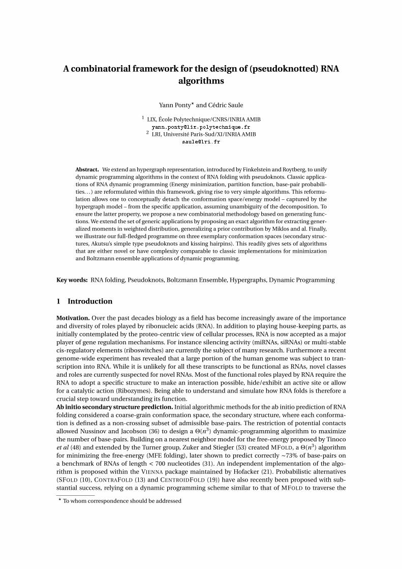
Fig. 1. Illustration of F-Graphs, F-Paths and Independence property. Straight lines indicate classic arcs, and bentcurves indicate hyperarcs.
on and revisit an hypergraph analogy proposed by Finkelstein et al (15) as a unifying framework for RNAfolding and other applications of Dynamic Programming in bioinformatics.Outline. In Section 2, we briefly remind some basic definitions related to forward directed hypergraphs.In Section 3, we remind and propose dynamic programming algorithms for generic problems on F-graphs. Then in Section 4, we illustrate our programme by proposing and proving unambiguous decom-positions for three space of conformations: Classic secondary structures in the Turner energy model (29),(weighted) base-pair maximisation version of Akutsu’s simple-type pseudoknots (1) and fully-recursivekissing hairpins (Unambiguous restriction of Chen et al (7)). We also describe a simplified proof strategybased on generating functions to prove the correctness of a given decomposition. Section 5 enriches thescope of applications of our framework by proposing a general algorithm for extracting the moments ofadditive features (free-energy, base-pairs, helices. . . ) in a weighted distribution (generalizing a previouscontribution by Miklos et al (35)). Finally Section 6 concludes with some remarks and possible extensionsand improvements.
2 Notations and key notions
Let us first remind that a directed hypergraph generalizes the notion of directed graph by allowing anynumber of vertices as origin(tail) and destination (head) for each (hyper)-arcs. We will be focusing hereon Forward-Hypergraphs, or F-graphs, which restrict the tail of their arcs to a single vertex.
Formally, let V be a set of vertices, an F-arc e = (t (e) → h(e)) ∈V ×P (V ), connects a single tail vertext (e) ∈ V to ordered list of vertices h(e) ⊆ V . An F-graph H = (V ,E) is characterized by a set of vertices Vand a set of F-arcs E . Denote by cn the children of a node in a tree, then an F-path of H = (V ,E) is a treeT = (V ′ ⊆V ,E ′) such that, for any node n ∈V ′, (vn → cn) ∈ E . For the sake of simplicity, we may omit theimplicit V ′ and denote an F-path by its set of edges E ′.
An F-derivation from a vertex s ∈ V can be recursively defined as either ⟨s,∅⟩ if (s → ∅) ∈ E , or⟨s,D1 . . . D |t|⟩ if (s → t) ∈ E and each Di is an F-derivation starting from ti . An F-graph is acyclic if andonly if any vertex s ∈ V is present only once (as a root) in any derivations starting from s. Moreover it isindependent if and only any vertex s ∈V is reached at most once in any derivation, regardless of its root.
A weighted F-graph is a triplet (V ,E ,π) such that (V ,E) is an F-graph and π : E → R+ is a weightfunction that associates a weight to each F-arc. Finally, an oriented F-graph is a quadruplet (v0,V ,E ,π)such that (V ,E ,π) is a weighted independent F-graph, and v0 ∈V is a distinguished initial vertex.
Remark 1: Notice that our definition of F-arcs and F-paths implicitly defines terminal vertices, since anyleaf l in a F-path has no child and our definition of F-paths therefore requires l →∅ to be an F-arc of H .
Remark 2: Under the independence property, the derivations starting from any node s ∈V are trees, andare therefore in bijection with F-paths originating from the same vertex.
3 Generic problems and algorithms for F-paths in F-graphs
In the following, terminal cases will very seldom appear explicitly, but will rather be captured by the limitcases of products
∏u∈∅ f (u) = 1 and sums
∑u∈∅ f (u) = 0, k ∈R.
Generating and counting F-paths in oriented F-graphs (52) Let H = (v0,V ,E ,π) be an oriented F-graph, we address the problem of generating the set Pv0 of F-paths obtained starting from v0.
From the tree-like definition of F-paths and our remark on terminal vertices, we know that any F-pathstarting from a vertex s can either a leaf, provided that there exists an F-arc s →∅, or an internal node.In the latter case, any F-paths is composed of auxiliary paths, generated from the vertices in the head ofsome F-edge having s as tail. Remark that our definition of F-paths requires each vertex from V to appearat most once in any F-path, a fact that is ensured here by the acyclicity of H . Therefore we can recursivelydefine the set of P s of F-paths starting from a root node s as
P s ={
{(s,∅)} If (s,∅) ∈ E∅ Otherwise
}∪ ⋃
(s→t)∈E
({s}×∏
u∈tPu
), ∀s ∈V. (1)
Since E is a set, the candidate heads for a given tail s are distinct and the unions in the above equationsare disjoint. Furthermore, the products are Cartesian, so we can directly transpose the recurrence aboveover the cardinalities ns = |P s | and obtain
ns = ∑(s→t)∈E
∏u∈t
nu , ∀s ∈V. (2)
This immediately yields a Θ(|V | + |E | +∑e∈E |h(e)|)/Θ(|V |) time/memory dynamic programming algo-
rithm for counting F-paths.
Minimal score F-path Let us consider an additive scoring scheme based on weights, and accordinglydefine the score of an F-path p to be α
(p
)=∑e∈E π(e). We address here the problem of finding an F-path
p0 having minimal score or more formally some p0 ∈ Pv0 such that ∀p ∈ Pv0 , p 6= p0 ⇒ α(p
) ≥ α(p0
).
From the independence of siblings and the strict additivity of the score, we know that the path minimiza-tion problem has optimal substructure, i. e. any optimal solution is composed of optimal solutions for itssubproblems. Consequently, the minimal score ms of a path starting from a root node s ∈V is given by
ms = mine=(s→t)∈E
(π(e)+∑
u∈tmu
), ∀s ∈V. (3)
A classic backtrack procedure can then be used to reconstruct the F-path instance pmins starting from
s ∈V and having minimal score. Alternatively, the previous recurrence can be modified as follows
pmins = argmin
p ′=⋃s′∈t pmin
s′s.t. (s→t)∈E
α({(s → t)}∪p ′) , ∀s ∈V , (4)
giving a Θ(|V |+ |E |+∑e∈E |h(e)|)/Θ(|V |) time/memory DP algorithm for the minimal weighted F-path.
Weighted count and weighted random generation (9) Let us extend multiplicatively on paths ourweight function, defining the weight of any F-path p to be π(p) = ∏
e∈p π(e). Then a small modifica-tion of Equation 2 gives a recurrence for computing the cumulated weight ws of F-paths starting from agiven vertex s.
ws = ∑p ′∈Pv0
π(p ′) = ∑e=(s→h(e))∈E
π(e) · ∏s′∈h(e)
ws′ , ∀s ∈V (5)
Provided that the weights are positive, this defines a weighted probability distribution over F-paths,which assigns to each path p ∈Pv0 a probability
P(p |π) = π(p)∑p ′∈Pv0
π(p ′)≡ π(p)
wv0
. (6)
From the precomputed values ws , one can perform a weighted random generation to draw at ran-dom a set of k F-paths from v0 according to a weighted distribution. Starting from any vertex s, the algo-rithm chooses at each step an F-arc e = (s → h(e)) with probability
ps,e =π(e) ·∏s′∈h(e) ws′
ws,
and proceeds to the recursive generation of auxiliary paths from each vertex in h(e). A simple inductionargument shows that any F-path is generated with respect to the probability distribution of Equation 6.The weighted count recurrence is computed by a Θ(|V | + |E | +∑
e∈E |h(e)|)/Θ(|V |) time/memory algo-rithm, and each generation of a path p can be achieved in Θ(|p|+∑
e∈p |h(e)|)/Θ(|p|) time/memory.
Remark 3: This worst-case complexity can be improved using additional information on the structure ofthe F-graph. For instance, when both the height and maximal degree of a vertex are bounded by someconstant n, Boustrophedon search (16; 38) can be used to decrease the worst-case complexity of eachgeneration from Θ(n2) to O (n logn).
Arc traversal probabilities Using the same probability distribution, a natural problem is to computethe probability pe of an F-arc e ∈ E being in a random F-path. To that purpose one can use the classicinside/outside algorithm, which can be rephrased as an F-graphs traversal.
Let us first point out that the probability pe is related to the cumulated weight of all F-paths featuringan edge e = (t (e) → h(e)) through
pe =
∑p∈Pv0s.t. e∈p
π(p)∑p ′∈Pv0
π(p ′)≡
∑p∈Pv0s.t. e∈p
π(p)
wv0
. (7)
From the independence of H , we know that each vertex appears at most once in any given F-path, andconsequently any F-path traversing e can therefore be unambiguously decomposed into: An e-outsidetree, i.e. a derivation from v0 whose leaves are either terminal or t (e), and which features exactly oneoccurrence of t (e); A support edge e = (t (e) → h(e)); An e-inside tree, i.e. a set of F-paths issued fromh(e).
The unambiguity of the decomposition, along with the independence of i) and iii), translates into∑p∈Pv0s.t. e∈p
π(p) = bt (e) ·π(e) · ∏s′∈h(e)
ws′ (8)
where bs is the cumulated weight of all outside trees leaving s ∈V underived. Finally it can be shown thatthe cumulated weight bs over all e-outside trees obey the following simple recurrence
bs = 1s=q0 +∑
e ′∈Es. t. s∈h(e ′)
π(e ′) ·bt (e ′) ·∏
s′∈h(e ′)s′ 6=s
ws′ , ∀s ∈V (9)
which can computed in O(|V |+ |E |+∑e∈E |h(e)|2)/Θ(|V |) time/memory. The probability of traversing pe
in a random F-path can finally be computed through the formula
pe =bt (e) ·∏s′∈h(e) ws′
wv0
, ∀e ∈ E . (10)
i
j
i
j-1
i
j
i j i j
i j
i+1 j-1i j
j-1
i'>i
i'>ij'<j
i j
j'<j
i j
i+1
i+1 j-1
k
i
jk
i
j
k
i
j
1 j
1 j-1 1 jk
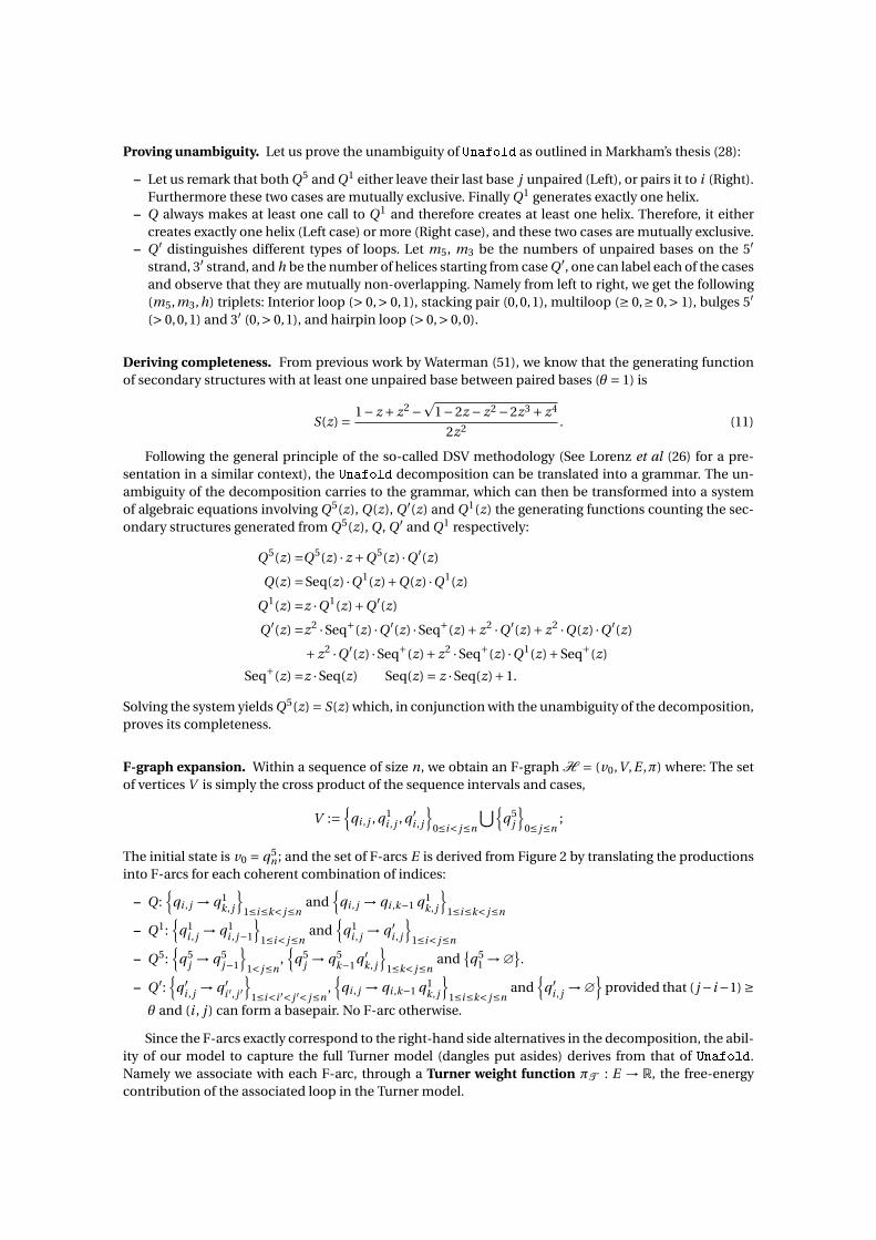
Fig. 2. Simplification of the Unafold (29) decomposition of the secondary structures space. Framed states indicateorigins of (hyper)arcs.
4 F-graphs reformulation of (Pseudoknotted) RNA folding search spaces
4.1 Foreword: Shortening correctness proofs through generating functions
Unambiguity is a necessary property for ensemble applications of dynamic programming, requiringeach element of the search space to be traversed (or equivalently generated) at most once. Since thisnotion is intimately related to the semantics associated to the F-paths, it cannot be tackled in an au-tomated way at the decomposition level3 but will usually require user-assigned semantics, from whichlocal disjointness can be asserted. On the other hand, the completeness of a decomposition requires tocover, or conversely generate, the entire search space. This property ensures that each element of thesearch space is traversed at most once. Again, completeness is usually proven in a non-automated wayby proving that any element of the search space can be parsed by the proposed decomposition.
Proving the correctness of ensemble DP schemes will typically require proving both completenessand unambiguity. Such a task may become challenging for complex decompositions. In order to simplifythe validation and therefore the design of new search spaces, we propose a proof technique based ongenerating functions. Indeed proving the correctness is equivalent to establishing that the structures SD
generated by the decomposition are in bijection with the targeted search space.However when information is available on cardinality for both the search space generated by the
decomposition and the targeted one, it is no longer necessary to prove both conditions, since one willnaturally imply the other. Therefore we propose an alternative approach based on generating functions.Namely S be the targeted search space, D be a decomposition, SD ⊂S the (multi)set of objects gener-ated from D, and | · | : S →N be a any (size) function. Let S(z) =∑
o∈S z |o| and SD(z) =∑o′∈SD
z |o′| be thegenerating functions of S and SD respectively, then the following proposition hold.
Proposition 1 (Completeness). Assume that D is unambiguous, then D is complete iff S(z) = SD(z).
Proposition 2 (Unambiguity). Assume that D is complete, then D is unambiguous iff S(z) = SD(z).
4.2 RNA secondary structures
Let us first illustrate our approach on RNA secondary structures, for which Unafold (29) – the successorof MFold (53) – offers an unambiguous scheme. Compared to the original decomposition presented inMarkham’s thesis (28), the one described in Figure 2 is simplified to ignore dangles.
3 Algebraic Dynamic Programming partially addresses this issue, and the interested reader is referred to an earlycontribution by Reeder et al (40).
Proving unambiguity. Let us prove the unambiguity of Unafold as outlined in Markham’s thesis (28):
– Let us remark that both Q5 and Q1 either leave their last base j unpaired (Left), or pairs it to i (Right).Furthermore these two cases are mutually exclusive. Finally Q1 generates exactly one helix.
– Q always makes at least one call to Q1 and therefore creates at least one helix. Therefore, it eithercreates exactly one helix (Left case) or more (Right case), and these two cases are mutually exclusive.
– Q ′ distinguishes different types of loops. Let m5, m3 be the numbers of unpaired bases on the 5′strand, 3′ strand, and h be the number of helices starting from case Q ′, one can label each of the casesand observe that they are mutually non-overlapping. Namely from left to right, we get the following(m5,m3,h) triplets: Interior loop (> 0,> 0,1), stacking pair (0,0,1), multiloop (≥ 0,≥ 0,> 1), bulges 5′(> 0,0,1) and 3′ (0,> 0,1), and hairpin loop (> 0,> 0,0).
Deriving completeness. From previous work by Waterman (51), we know that the generating functionof secondary structures with at least one unpaired base between paired bases (θ = 1) is
S(z) = 1− z + z2 −p
1−2z − z2 −2z3 + z4
2z2 . (11)
Following the general principle of the so-called DSV methodology (See Lorenz et al (26) for a pre-sentation in a similar context), the Unafold decomposition can be translated into a grammar. The un-ambiguity of the decomposition carries to the grammar, which can then be transformed into a systemof algebraic equations involving Q5(z), Q(z), Q ′(z) and Q1(z) the generating functions counting the sec-ondary structures generated from Q5(z), Q, Q ′ and Q1 respectively:
Solving the system yields Q5(z) = S(z) which, in conjunction with the unambiguity of the decomposition,proves its completeness.
F-graph expansion. Within a sequence of size n, we obtain an F-graph H = (v0,V ,E ,π) where: The setof vertices V is simply the cross product of the sequence intervals and cases,
V :={
qi , j , q1i , j , q ′
i , j
}0≤i< j≤n
⋃{q5
j
}0≤ j≤n
;
The initial state is v0 = q5n ; and the set of F-arcs E is derived from Figure 2 by translating the productions
into F-arcs for each coherent combination of indices:
– Q:{
qi , j → q1k, j
}1≤i≤k< j≤n
and{
qi , j → qi ,k−1 q1k, j
}1≤i≤k< j≤n
– Q1:{
q1i , j → q1
i , j−1
}1≤i< j≤n
and{
q1i , j → q ′
i , j
}1≤i< j≤n
– Q5:{
q5j → q5
j−1
}1< j≤n
,{
q5j → q5
k−1q ′k, j
}1≤k< j≤n
and{
q51 →∅
}.
– Q ′:{
q ′i , j → q ′
i ′, j ′}
1≤i<i ′< j ′< j≤n,{
qi , j → qi ,k−1 q1k, j
}1≤i≤k< j≤n
and{
q ′i , j →∅
}provided that ( j −i−1) ≥
θ and (i , j ) can form a basepair. No F-arc otherwise.
Since the F-arcs exactly correspond to the right-hand side alternatives in the decomposition, the abil-ity of our model to capture the full Turner model (dangles put asides) derives from that of Unafold.Namely we associate with each F-arc, through a Turner weight function πT : E → R, the free-energycontribution of the associated loop in the Turner model.
Application Algorithm Weight fun. Time Memory Ref.
A – Energy minimization Minimal weight πT O(n3) O(n2) (53)
B – Partition function Weighted count e−πT
RT O(n3) O(n2) (32)
C – Base-pairing probabilities Arc-traversal prob. e−πT
RT O(n3) O(n2) (32)
D – Statistical sampling (k-samples) Weighted random gen. e−πT
RT O(n3 +k ·n logn) O(n2) (11; 38)
E – Moments of energy (Mean, Var.) Moments extraction e−πT
RT O(n3) O(n2) (35)
F – m-th moment of additive features Moments extraction e−πT
RT O(m3.n3) O(m.n2) –
G – Correlations of additive features Moments extraction e−πT
RT O(n3) O(n2) –
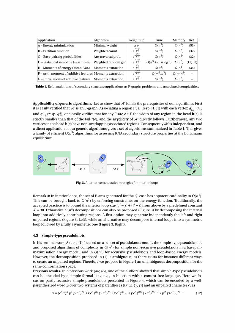
Table 1. Reformulations of secondary structure applications as F-graphs problems and associated complexities.
Applicability of generic algorithms. Let us show that H fulfills the prerequisites of our algorithms. Firstit is easily verified that H is an F-graph. Associating a region [i , j ] (resp. [1, j ]) with each vertex q1
i , j , qi , j
and q ′i , j (resp. q5
j ), one easily verifies that for any F-arc e ∈ E the width of any region in the head h(e) is
strictly smaller than that of the tail t (e), and the acyclicity of H directly follows. Furthermore, any twovertices in the head h(e) have non-overlapping associated regions. Consequently H is independent, anda direct application of our generic algorithms gives a set of algorithms summarized in Table 1. This givesa family of efficient O(n3) algorithms for assessing RNA secondary structure properties at the Boltzmannequilibrium.
Alt. 1 Alt. 2i j
i j
i+k j-k
i+k
l j-k
j-k
l>i+k
i j
kkl
i
Fig. 3. Alternative exhaustive strategies for interior loops.
Remark 4: In interior loops, the set of F-arcs generated for the Q ′ case has apparent cardinality in O(n4).This can be brought back to O(n3) by enforcing constraints on the energy function. Traditionally, theaccepted practice is to bound the interior loop size ( j ′− j )+ (i ′− i ) from above by a predefined constantK = 30. Exhaustive O(n3) decompositions can also be proposed (Figure 3) by decomposing the internalloop into additively-contributing regions. A first option may generate independently the left and rightunpaired regions (Figure 3, Left), while an alternative may decompose internal loops into a symmetricloop followed by a fully asymmetric one (Figure 3, Right).
4.3 Simple-type pseudoknots
In his seminal work, Akutsu (1) focused on a subset of pseudoknots motifs, the simple-type pseudoknots,and proposed algorithms of complexity in O(n4) for simple non-recursive pseudoknots in a basepair-maximisation energy model, and in O(n5) for recursive pseudoknots and loop-based energy models.However, the decomposition proposed in (1) is ambiguous, as there exists for instance different waysto create an unpaired regions. Therefore we propose in Figure 4 an unambiguous decomposition for thesame conformation space.Previous results. In a previous work (44; 45), one of the authors showed that simple-type pseudoknotscan be encoded by a simple formal language, in bijection with a context-free language. Here we fo-cus on partly recursive simple pseudoknots presented in Figure 4, which can be encoded by a well-parenthesized word p over two systems of parentheses {(x, x), (y, y)} and an unpaired character c, as
p = (c∗x)n p ′ (y c∗)m1 (x c∗)n1 (y c∗)m2 (x c∗)n2 · · · (y c∗)mk (x c∗)nk−1 x p ′′ y (c∗ y)m−1 (12)
a x b
i
a x b
i
a x b
i
a x b
i
a x b
i
a
b=j-1
i
k j
Entry point
x=k+1
ji
a x b
i
b-1x+1i
a
a-1 x+1b
i
i j
i j
i ji k k+1 jExit Point
a=i
k j
x
b=x
a=i
a=i
k j
b=x
Fig. 4. An unambiguous decomposition for simple non-recursive pseudoknots that captures the Akutsu/Uemuraclass of pseudoknots. This decomposition yields O(n4)/Θ(n4) time/memory algorithms for partially recursive pseu-doknots and can be extended to include recursive pseudoknots and/or Turner energy contributions in O(n5)/Θ(n4).
where k is some integral value,∑k
i=1 ni = n ≥ 1,∑k
i=1 mi = m ≥ 1, and p ′, p ′′ are any two recursively-generated conformations.Completeness. Let us show that the decomposition in Figure 4 is complete, i.e. that any partially recur-sive pseudoknot can be generated by the decomposition.
Let us initially focus on base-pairs and ignore unpaired bases. The smallest word within the languageof Equation 12 is xp ′y xp ′′ y which can be generated by applying the initial case (Q → AL → AM → A p ′ . . . y . . . y) followed directly by the terminal case (A → AT x p ′ y x p ′′ y). Moreover through a sequenceA → AR → AM → A, one adds an outermost edge around the right part y . . . y . So through m iterationsof the sequence the decomposition generates any structure ym1 . . . ym1 . Similarly through a sequenceA → AL → AM → A one adds an outermost edge around the left part x . . . x, and after n1 iterations anystructure xn1 . . . xn1 is generated. Since these two sequences can be combined and alternated (startingwith the initial case and finishing with the terminal case), then the decomposition generates any word
p = xn p ′ ym1 xn1 ym2 xn2 · · · ymk xnk p ′′ ym y . (13)
For the recursive call p ′, it is easily verified that Q∗ generates any (PK) structure. For p ′′ it is worth men-tioning that, at a base-pairing level, A → AT (right base paired) and A →; cover all possible situations.
Arbitrary numbers of unpaired bases c can also be inserted right before the opening x of a leftwardbase pair (resp. after closure x of a leftward base pair, after the opening y of a right base pair and beforethe closure y of a right base pair) by repeatedly applying the AL → AL (resp. AM → AM , AL → AL andAM → AM ) rule after adding a left (resp. right) base pair. Consequently any structure described by a wordin Equation 12 can be generated by the decomposition.Unambiguity. Let us now address the unambiguity of the decomposition, using our approach based ongenerating functions. Equation 12 immediately gives a system of equations relating AU (z), the generatingfunction of simple partially recursive pseudoknots, to S(z) the gen. fun. of all structures:
AU (z) = ∑k≥1
( z
1− z
)nS(z)
( z
1− z
)m1( z
1− z
)n1 · · ·( z
1− z
)nk−1z S(z) z
( z
1− z
)m−1= z4 S(z)2 (1− z)
1−2 z − z2 .
Now consider the dynamic programming decomposition illustrated by Figure 4. Associating generatingfunctions to each type of vertices and translating assigned bases into monomials, we obtain the followingsystem of equations:
Q ′(z) = z2 S(z) AR (z) AL(z) = z AL(z)+ AM (z) AR (z) = z AR (z)+ AM (z)
AM (z) = z AM (z)+ A(z) A(z) = z2 AR (z)+ z2 AL(z)+ z2 S(z) AT (z) = S(z)(1− z)−1.
ji
i jk l i jk l
i jk l
i jk l i jk l
i jk l
Entry Point
i jk l
i
j
l mk
mjk l
ii
jlm
k
i jk
l
mi jk
l
m
ijlm
k
i k
l j
Exit Point
Fig. 5. Unambiguous decomposition of fully recursive kissing hairpins.
The last expression for AT (z) follows directly from the observation that any structure in Q can be writtenas a sequence of structures from Q ′ interleaved with sequences of unpaired bases. Given that AT cannotfeature unpaired bases on its right end, one of the sequence of unpaired base must be removed. Further-more AT does not generate the empty structure, so we have S(z) = (AT (z)+1)/(1−z). Solving the system
gives Q ′(z) = S2(z) z4 (1−z)1−2 z+z2 = AU (z) and the unambiguity/correctness of the decomposition directly follow.
4.4 Fully-recursive kissing hairpins
Kissing hairpins (KH) are pseudoknotted structure composed of two helices whose terminal loops arelinked by a third helix. These pseudoknots are frequently observed, and are exhaustively predicted byChen et al (7) in time complexity in O(n5), and in O(n3)/O(n4) under restrictions by Theis et al (47). Fig-ure 5 presents an unambiguous decomposition which generates the space of recursive kissing hairpins.Previous results. Again, an encoding of kissing hairpins can be found in earlier work by one of the au-thors (44), showing that any KH pseudoknot can be represented by a word p over three systems of paren-theses {(x, x), (y, y), (z, z)} (respectively denoting leftmost, central and rightmost helices) such that:
p = (xS)n (yS)m (xS)n (zS)k (yS)m (zS)k−1 z. (14)
Completeness. First let us remark that the minimal conformation generated by the decomposition isKL → KR → K ′
R → KM xSySxSzS ySz. Remark that one can iterate arbitrarily over the states KL →K ′
L → KL , K ′R → KR → K ′
R and K ′M → KM → KM . Consequently one may insert patterns (KL → K ′
L →KL)n−1 (S x)n−1 · · · (x S)n−1, (K ′
R → KR → K ′R )k−1 (z S)k−1 · · · (z S)k−1 and (KM → K ′
M → KM )m (y S)m−1 · · · (S y)m−1 in the minimal word above, and produce any conformation denoted by
x(Sx)n−1S(yS)m−1 yS(xS)n−1xSzS(zS)k−1 y(S y)m−1S(zS)k−1 z
where one recognizes the language of Equation 14 upon simple refactorization.Unambiguity. Equation 14 allows to derive the generating function K H(z) of kissing-hairpin as a func-tion of S(z) the gen. fun. of all structures:
A – Energy minimization Minimal weight πT O(n5) O(n4) (7)
B – Partition function Weighted count e−πT
RT O(n5) O(n4) –
C – Base-pairing probabilities Arc-traversal prob. e−πT
RT O(n5) O(n4) –
D – Statistical sampling (k-samples) Weighted rand. gen. e−πT
RT O(n5 +k ·n logn) O(n4) –
E – Moments of energy (Mean, Var.) Moments extraction e−πT
RT O(n5) O(n4) –
F – m-th moment of additive features Moments extraction e−πT
RT O(m3.n5) O(m.n4) –
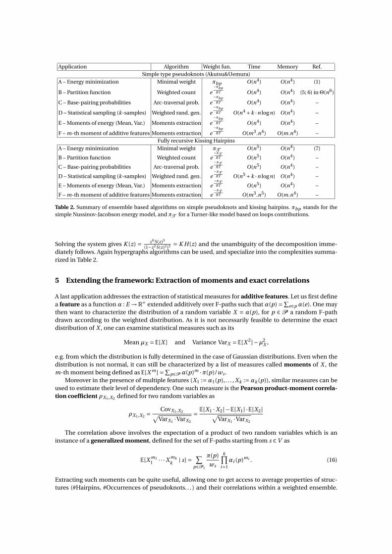
Table 2. Summary of ensemble based algorithms on simple pseudoknots and kissing hairpins. πbp stands for thesimple Nussinov-Jacobson energy model, and πT for a Turner-like model based on loops contributions.
Solving the system gives K (z) = z6S(z)5
(1−z2S(z)2)3 = K H(z) and the unambiguity of the decomposition imme-diately follows. Again hypergraphs algorithms can be used, and specialize into the complexities summa-rized in Table 2.
5 Extending the framework: Extraction of moments and exact correlations
A last application addresses the extraction of statistical measures for additive features. Let us first definea feature as a function α : E →R+ extended additively over F-paths such that α(p) =∑
e∈p α(e). One maythen want to characterize the distribution of a random variable X = α(p), for p ∈ P a random F-pathdrawn according to the weighted distribution. As it is not necessarily feasible to determine the exactdistribution of X , one can examine statistical measures such as its
Mean µX = E[X ] and Variance VarX = E[X 2]−µ2X ,
e.g. from which the distribution is fully determined in the case of Gaussian distributions. Even when thedistribution is not normal, it can still be characterized by a list of measures called moments of X , them-th moment being defined as E[X m] =∑
p∈P α(p)m ·π(p)/ws .Moreover in the presence of multiple features (X1 :=α1(p), . . . , Xk :=αk (p)), similar measures can be
used to estimate their level of dependency. One such measure is the Pearson product-moment correla-tion coefficient ρX1,X2 defined for two random variables as
ρX1,X2 =CovX1,X2√
VarX1 ·VarX2
= E[X1 ·X2]−E[X1] ·E[X2]√VarX1 ·VarX2
The correlation above involves the expectation of a product of two random variables which is aninstance of a generalized moment, defined for the set of F-paths starting from s ∈V as
E[X m11 · · ·X mk
k | s] = ∑p∈P s
π(p)
ws
k∏i=1
αi (p)mi . (16)
Extracting such moments can be quite useful, allowing one to get access to average properties of struc-tures (#Hairpins, #Occurrences of pseudoknots. . . ) and their correlations within a weighted ensemble.
For instance, Miklos et al (35) proposed an O (m2 · n3) algorithm for computing the m-th moment ofthe Energy distribution for secondary structure in order to compare the distribution of free-energy innon-coding RNAs and random sequences. We are going to show how these generalized moments can beextracted directly through a generalization of the weighted count algorithm.
Theorem 1. Let α := (α1, · · · ,αk ) be a vector of additive features and m := (m1, · · · ,mk ) be a k-uplet ofnatural integers. Then the pseudo-moment cm
s := E[X m11 · · ·X mk
k | s] ·ws of α in a weighted distribution canbe recursively computed through
cms = ∑
e=(s→t)π(e) · ∑
m′,(m′′
1 ,··· ,m′′|t |
)s. t. m′+∑
j m′′j =m
k∏i=1
(mi
m′i ,m′′
1,i , · · · ,m′′|t |,i
)·αi (e)m′
i ·|t |∏
i=1c
m′′i
ti(17)
in O((|E |+ |V |) ·k · t+ ·∏k
i=1 mt++1i
)time complexity andΘ
(|V | ·∏ki=1 mi
)memory where t+ = max(s→t )∈E (|t |)
is the maximal out-degree of an arc.
Adding this new generic algorithms automatically creates new applications for each an every confor-mation space as summarized in Figure 2. This simultaneous extension – for all conformational spaces– of possible ensemble applications constitues in our opinion one of the main benefit of detaching thedecomposition from its traversal/generation.
6 Conclusion and Perspectives
In this paper, we established the foundation of a combinatorial approach to the design of algorithmsfor complex conformation spaces. We built on an hypergraph model introduced in the context of RNAsecondary structure by Finkelstein and Roytberg (15), which we extended in several direction. First weformulated classic and novel generic algorithms on Forward-Hypergraphs for weighted ensembles, al-lowing one to derive base-pairing probabilities, perform statistical sampling and extract moments of thedistribution of additive features. Then we showed how combinatorial arguments based on generatingfunctions could be used to simplify the proof of correctness for designed decompositions. We illustratedthe full programme on classic secondary structures, simple type pseudoknots and fully-recursive kiss-ing hairpin pseudoknots for which we provided decompositions that were proven to be unambiguousand complete with respect to previous work. The hypergraph formulation of the decomposition, cou-pled with the generic algorithms, readily gave a family of novel algorithms for complex – yet relevant –conformation spaces.
There exists many perspectives to our contribution. First the principles and algorithms describedhere could easily be implemented as a general compiler tools for Forward-Hypergraph algorithms. Such acompiler could be coupled with helper tools expanding hypergraphs from succinct descriptions. Some ofthe candidates for such descriptions are context-free grammars (related to ADP (18)), or Matthias Möhl’ssplit types (34). More complex search space could also be modeled, such as those relying on a moredetailed representation of RNA structure (e.g. MCFold’s NCMs (37)), those capturing RNA-RNA interac-tions (2; 23), those offering simultaneous alignment and folding (Sankoff’s algorithm (43)) or performingmutations on the sequence (50). Finally hypergraph algorithms are not necessarily limited to dynamic-programming, and algorithmic developments could be proposed to address some of the current algo-rithmic issues in RNA (inverse folding (3), kinetics (46)) for which no exact polynomial algorithms arecurrently known. More generally it is our hope that, by simplifying and modularizing the process of de-veloping new – algorithmically tractable – conformation spaces, our contribution will help design better,more topologically-realistic(49; 25; 41), energy and conformational spaces to better understand and pre-dict the structure(s) of RNA.
Acknowledgement
The authors wish to express their gratitude to M. Roytberg for pointing out his work on hypergraphs as aunifying framework, and to R. Backofen, M. Möhl and S. Will for fruitful discussions.
Bibliography
[1] Akutsu, T.: Dynamic programming algorithms for RNA secondary structure prediction with pseudoknots. Discrete Appl. Math. 104(1-3), 45–62(2000)
[2] Alkan, C., Karakoç, E., Nadeau, J.H., Sahinalp, S.C., Zhang, K.: RNA-RNA Interaction Prediction and Antisense RNA Target Search. In: Proceed-ings of RECOMB’05 (2005)
[3] Andronescu, M., Fejes, A.P., Hutter, F., Hoos, H.H., Condon, A.: A New Algorithm for RNA Secondary Structure Design. J Mol Biol 336(3), 607–624(2004)
[4] Bekaert, M., Bidou, L., Denise, A., Duchateau-Nguyen, G., Forest, J., Froidevaux, C., Hatin, I., Rousset, J., Termier, M.: Towards a computationalmodel for −1 eukaryotic frameshifting sites. Bioinformatics 19, 327–335 (2003)
[5] Cao, S., Chen, S.J.: Predicting RNA pseudoknot folding thermodynamics. Nucleic Acids Res 34(9), 2634–2652 (2006)[6] Cao, S., Chen, S.J.: Predicting structured and stabilities for H-type pseudoknots with interhelix loop. RNA 15, 696–706 (2009)[7] Chen, H.L., Condon, A., Jabbari, H.: An O(n(5)) algorithm for MFE prediction of kissing hairpins and 4-chains in nucleic acids. Journal of
(2004)[9] Denise, A., Ponty, Y., Termier, M.: Controlled non uniform random generation of decomposable structures. Theoretical Computer Science
411(40-42), 3527–3552 (September 2010)[10] Ding, Y., Chan, C.Y., Lawrence, C.E.: RNA secondary structure prediction by centroids in a boltzmann weighted ensemble. RNA 11, 1157–1166
(2005)[11] Ding, Y., Lawrence, E.: A statistical sampling algorithm for RNA secondary structure prediction. Nucleic Acids Res 31(24), 7280–7301 (2003)[12] Dirks, R., Pierce, N.: A partition function algorithm for nucleic acid secondary structure including pseudoknots. J Comput Chem 24, 1664–1677
e90–e98 (Jul 2006)[14] Ferrè, F., Ponty, Y., Lorenz, W.A., Clote, P.: DIAL: A web server for the pairwise alignment of two RNA 3-dimensional structures using nucleotide,
dihedral angle and base pairing similarities. Nucleic Acids Res (35 (Web server issue)), W659–668 (July 2007)[15] Finkelstein, A.V., Roytberg, M.A.: Computation of biopolymers: a general approach to different problems. Biosystems 30(1-3), 1–19 (1993)[16] Flajolet, P., Zimmermann, P., Van Cutsem, B.: Calculus for the random generation of labelled combinatorial structures. Theoretical Computer
Science 132, 1–35 (1994), a preliminary version is available in INRIA Research Report RR-1830[17] Flajolet, P.: Analytic models and ambiguity of context-free languages. Theoretical Computer Science 49, 283–309 (1987)[18] Giegerich, R.: A systematic approach to dynamic programming in bioinformatics. Bioinformatics 16(8), 665–677 (Aug 2000)[19] Hamada, M., Kiryu, H., Sato, K., Mituyama, T., Asai, K.: Prediction of RNA secondary structure using generalized centroid estimators. Bioinfor-
matics 25(4), 465–473 (Feb 2009)[20] Harmanci, A.O., Sharma, G., Mathews, D.H.: Stochastic sampling of the rna structural alignment space. Nucleic Acids Res 37(12), 4063–4075
26(2), 175–181 (Jan 2010), http://dx.doi.org/10.1093/bioinformatics/btp635[24] Lefebvre, F.: A grammar-based unification of several alignment and folding algorithms. In: Proceedings of the Fourth International Conference
on Intelligent Systems for Molecular Biology. pp. 143–154. AAAI Press (1996)[25] Lescoute, A., Westhof, E.: Topology of three-way junctions in folded RNAs. RNA 12(1), 83–93 (2006)[26] Lorenz, W., Ponty, Y., Clote, P.: Asymptotics of RNA shapes. Journal of Computational Biology 15(1), 31–63 (Jan–Feb 2008)[27] Lyngsø, R.B., Pedersen, C.N.S.: RNA pseudoknot prediction in energy-based models. Journal of Computational Biology 7(3-4), 409–427 (2000)[28] Markham, N.R.: Algorithms and software for nucleic acid sequences. Ph.D. thesis, Faculty of Rensselaer Polytechnic Institute (2006)[29] Markham, N.R., Zuker, M.: UNAFold: software for nucleic acid folding and hybridization. Methods Mol Biol 453, 3–31 (2008)[30] Mathews, D.H.: Using an RNA secondary structure partition function to determine confidence in base pairs predicted by free energy mini-
mization. RNA 10(8), 1178–1190 (2004)[31] Mathews, D., Sabina, J., Zuker, M., Turner, D.: Expanded sequence dependence of thermodynamic parameters improves prediction of RNA
secondary structure. J Mol Biol 288, 911–940 (1999)[32] McCaskill, J.: The equilibrium partition function and base pair binding probabilities for RNA secondary structure. Biopolymers 29, 1105–1119
(1990)[33] Mückstein, U., Hofacker, I.L., Stadler, P.F.: Stochastic pairwise alignments. Bioinformatics 18 Suppl 2, S153–S160 (2002)[34] Möhl, M., Will, S., Backofen, R.: Lifting prediction to alignment of rna pseudoknots. J Comput Biol 17(3), 429–442 (Mar 2010), http://dx.
doi.org/10.1089/cmb.2009.0168
[35] Miklós, I., Meyer, I.M., Nagy, B.: Moments of the boltzmann distribution for RNA secondary structures. Bull Math Biol 67(5), 1031–1047 (Sep2005)
[36] Nussinov, R., Jacobson, A.B.: Fast algorithm for predicting the secondary structure of single stranded RNA. Proc. Natl. Acad. Sci. U. S. A. 77(11),6309–6313 (1980)
[37] Parisien, M., Major, F.: The MC-Fold and MC-Sym pipeline infers RNA structure from sequence data. Nature 452(7183), 51–55 (2008)[38] Ponty, Y.: Efficient sampling of RNA secondary structures from the boltzmann ensemble of low-energy: The boustrophedon method. J Math
Biol 56(1-2), 107–127 (Jan 2008)[39] Reeder, J., Giegerich, R.: Design, implementation and evaluation of a practical pseudoknot folding algorithm based on thermodynamics. BMC
[42] Rivas, E., Eddy, S.: A dynamic programming algorithm for RNA structure prediction including pseudoknots. J Mol Biol 285, 2053–2068 (1999)[43] Sankoff, D.: Simultaneous solution of the rna folding, alignment and protosequence problems. SIAM J Appl Math 45, 810–825 (1985)[44] Saule, C.: Modèles combinatoires des structures d’ARN avec ou sans pseudonœuds, application à la comparaison de structures. Ph.D. thesis,
Université Paris Sud, Ecole doctorale informatique. (December 2010)[45] Saule, C., Régnier, M., Steyaert, J.M., Denise, A.: Counting RNA pseudoknotted structures. Journal of Computational Biology (To appear)[46] Thachuk, C., Manuch, J., Rafiey, A., Mathieson, L.A., Stacho, L., Condon, A.: An algorithm for the energy barrier problem without pseudoknots
and temporary arcs. Pac Symp Biocomput pp. 108–119 (2010)[47] Theis, C., Janssen, S., Giegerich, R.: Prediction of rna secondary structure including kissing hairpin motifs. In: Proceedings of WABI 2010. pp.
52–64 (2010)[48] Tinoco, I., Borer, P.N., Dengler, B., Levin, M.D., Uhlenbeck, O.C., Crothers, D.M., Bralla, J.: Improved estimation of secondary structure in
ribonucleic acids. Nat New Biol 246(150), 40–41 (Nov 1973)[49] Vernizzi, G., Ribeca, P., Orland, H., Zee, A.: Topology of pseudoknotted homopolymers. Physical Review E (Statistical, Nonlinear, and Soft Matter
(2008), http://dx.doi.org/10.1371/journal.pcbi.1000124[51] Waterman, M.S.: Secondary structure of single stranded nucleic acids. Advances in Mathematics Supplementary Studies 1(1), 167–212 (1978)[52] Wilf, H.S.: A unified setting for sequencing, ranking, and selection algorithms for combinatorial objects. Advances in Mathematics 24, 281–291
(1977)[53] Zuker, M., Stiegler, P.: Optimal computer folding of large RNA sequences using thermodynamics and auxiliary information. Nucleic Acids Res
9, 133–148 (1981)
Proof of Theorem 1
Lemma 1. Let {xi , j }1≤i≤N1≤ j≤M
be a set of N × M real-valued coefficients, and (ai )1≤i≤N ∈ NN be a tuple of
integer exponents. Furthermore let us remind the multinomial notation(a
b1,b2, · · · ,bM
)= a!
b1!b2! · · ·bM !.
Then the following identity holds
N∏i=1
(M∑
j=1xi , j
)ai
= ∑b1:=(b1,1,··· ,b1,M )···
bN :=(bN ,1,··· ,bN ,M )s.t.
∑Mj=1 bi , j =ai ,∀i∈[1,N ]
N∏i=1
((ai
bi ,1, · · · ,bi ,M
)M∏
j=1x
bi , j
i , j
)(18)
Proof. To prove Equation 18, we are going to proceed by induction on N . For N = 1, Equation 18 special-izes into
in which one recognizes the multinomial coefficients formula.Assume that Equation 18 holds for N = K −1. Then for N = K , one has
K∏i=1
(M∑
j=1xi , j
)ai
=K−1∏i=1
(M∑
j=1xi , j
)ai
×(
M∑j=1
xk, j
)ak
=
∑(b1,··· ,bK−1),∑M
j=1 bi , j =ai
K−1∏i=1
(ai
bi ,1, · · · ,bi ,M
)M∏
j=1x
bi , j
i , j
×(
M∑j=1
xk, j
)ak
.
The right-hand side term of the product can be developed using the multinomial coefficients formula,and it follows that
K∏i=1
(M∑
j=1xi , j
)ai
=
∑(b1,··· ,bK−1),∑M
j=1 bi , j =ai
K−1∏i=1
(ai
bi ,1, · · · ,bi ,M
)M∏
j=1x
bi , j
i , j
×
∑bK s. t.∑M
j=1 bK , j =aK
(aK
bK ,1, · · · ,bK ,M
)M∏
j=1x
bK , j
K , j
.
Since the two terms of the highest-level product are mutually independent, we can treat the right-handas a constant and inject it within the left-hand sum.
K∏i=1
(M∑
j=1xi , j
)ai
= ∑(b1,··· ,bK−1),∑M
j=1 bi , j =ai
∑
bK s. t.∑Mj=1 bK , j =aK
(aK
bK ,1, · · · ,bK ,M
)M∏
j=1x
bK , j
K , j
×K−1∏i=1
(ai
bi ,1, · · · ,bi ,M
)M∏
j=1x
bi , j
i , j
This argument can be used to inject the right-hand-side products within the inner sum. It follows that
K∏i=1
(M∑
j=1xi , j
)ai
= ∑(b1,··· ,bK−1),∑M
j=1 bi , j =ai
∑bK s. t.∑M
j=1 bK , j =aK
((aK
bK ,1, · · · ,bK ,M
)M∏
j=1x
bK , j
K , j
K−1∏i=1
(ai
bi ,1, · · · ,bi ,M
)M∏
j=1x
bi , j
i , j
)
= ∑(b1,··· ,bK−1),∑M
j=1 bi , j =ai
∑bK s. t.∑M
j=1 bK , j =aK
(K∏
i=1
(ai
bi ,1, · · · ,bi ,M
)M∏
j=1x
bi , j
i , j
)
= ∑(b1,··· ,bK ),∑M
j=1 bi , j =ai
(K∏
i=1
(ai
bi ,1, · · · ,bi ,M
)M∏
j=1x
bi , j
i , j
).
So the validity of the initial statement for N = K −1 implies its validity for N = K which, in combinationwith its initial validity at N = 0, implies the universal validity of the identity. ut
Theorem 2. Let m := (m1, · · · ,mk ) be a k-uplet of natural integers.Then the pseudo-moment cm
s := E[X m11 · · ·X mk
k | s] ·ws can be recursively computed through
cms = ∑
e=(s→t)π(e) · ∑
m′,(m′′
1 ,··· ,m′′|t |
)s. t. m′+∑
j m′′j =m
k∏i=1
(mi
m′i ,m′′
1,i , · · · ,m′′|t |,i
)·αi (e)m′
i ·|t |∏
i=1c
m′′i
ti. (19)
Proof. Since the F-graph is acyclic, one can use a bottom-up induction, starting from vertices s∗ at height0, i.e. having only terminal edges. For such nodes, Equation 19 simplifies into
cms∗ =
∑e=(s∗→∅)
π(e) ·k∏
i=1
(mi
mi
)·αi (e)mi = ∑
e=(s∗→∅)π(e) ·
k∏i=1
αi (e)mi = ∑p∈P s∗
π(p) ·k∏
i=1αi (p)mi
in which one recognizes the definition of the pseudo-moment.Let us now assume that Equation 19 was able to compute the pseudo-moments for any outgoing
vertex of s. It follows that, for any such vertex ti and any k-uplet of integers m′′i , one has
cm′′
iti
= ∑pi∈P ti
π(pi ) ·k∏
j=1α j (pi )
m′′j
|t |∏i=1
cm′′
iti
=|t |∏
i=1
∑pi∈P ti
π(pi ) ·k∏
j=1α j (pi )
m′′j
= ∑(p1,··· ,p|t |)s.t. pi∈P ti
(( |t |∏i=1
π(pi )
)×
|t |∏i=1
k∏j=1
α j (pi )m′′
i , j
).
Now applying the formula of Equation 19 to a vertex s, one obtains
cms = ∑
e=(s→t)π(e) · ∑
m′,(m′′
1 ,··· ,m′′|t |
)s. t. m′+∑
j m′′j =m
(k∏
i=1
(mi
m′i ,m′′
1,i , · · · ,m′′|t |,i
)·αi (e)m′
i
) ∑(p1,··· ,p|t |)s.t. pi∈P ti
(( |t |∏i=1
π(pi )
)×
|t |∏i=1
k∏j=1
α j (pi )m′′
i , j
)
= ∑e=(s→t)
π(e) · ∑m′,
(m′′
1 ,··· ,m′′|t |
)s. t. m′+∑
j m′′j =m
∑(p1,··· ,p|t |)s.t. pi∈P ti
((k∏
i=1
(mi
m′i ,m′′
1,i , · · · ,m′′|t |,i
)·αi (e)m′
i
)( |t |∏i=1
π(pi )
)×
|t |∏i=1
k∏j=1
α j (pi )m′′
i , j
).
Since the sums on (m′,m′′) and (p1, · · · , p|t |) are mutually independent, their order of summation canbe exchanged. Furthermore the π(·) terms do not depend on (m′,m′′) and (p1, · · · , p|t |), so they can bemoved out of the summations.
cms = ∑
e=(s→t)π(e) · ∑
(p1,··· ,p|t |)s.t. pi∈P ti
∑m′,
(m′′
1 ,··· ,m′′|t |
)s. t. m′+∑
j m′′j =m
((k∏
i=1
(mi
m′i ,m′′
1,i , · · · ,m′′|t |,i
)·αi (e)m′
i
)( |t |∏i=1
π(pi )
)×
|t |∏i=1
k∏j=1
α j (pi )m′′
i , j
)
= ∑e=(s→t)
· ∑(p1,··· ,p|t |)s.t. pi∈P ti
π(e)
( |t |∏i=1
π(pi )
) ∑m′,
(m′′
1 ,··· ,m′′|t |
)s. t. m′+∑
j m′′j =m
((k∏
i=1
(mi
m′i ,m′′
1,i , · · · ,m′′|t |,i
)·αi (e)m′
i
)×
|t |∏i=1
k∏j=1
α j (pi )m′′
i , j
)
= ∑e=(s→t)
∑(p1,··· ,p|t |)s.t. pi∈P ti
π(e)
( |t |∏i=1
π(pi )
) ∑m′,
(m′′
1 ,··· ,m′′|t |
)s. t. m′+∑
j m′′j =m
k∏i=1
((mi
m′i ,m′′
1,i , · · · ,m′′|t |,i
)×αi (e)m′
i ×|t |∏
j=1αi (p j )
m′′j ,i
).
From a direct application of Lemma 1, we have
k∏i=1
((mi
m′i ,m′′
1,i , · · · ,m′′|t |,i
)×αi (e)m′
i ×|t |∏
j=1αi (p j )
m′′j ,i
)=
k∏i=1
(αi (e)+
|t |∑j=1
αi (p j )
)mi
and it follows that
cms = ∑
e=(s→t)
∑(p1,··· ,p|t |)s.t. pi∈P ti
(π(e)
|t |∏i=1
π(pi )
)k∏
i=1
(αi (e)+
|t |∑j=1
αi (p j )
)mi
.
At this point, let us make a few observations to conclude. Consider an F-path p, starting with an F-arce = (s → t), followed by |t | F-paths (p1, · · · , p|t |) such that pi ∈P ti ,∀i ∈ [1, |t |]:
– From the multiplicative definition of the weight, we know that π(p) =π(e)∏|t |
i=1π(pi ).
– From the additive definition of features, we know that α j (p) =α j (e)+∑|t |i=1α j (pi ).
– Any path originating from s can be uniquely decomposed as an edge followed by a tuple of pathsoriginating from its outgoing edges.
It follows that
cms = ∑
p∈P s
π(p)×k∏
i=1αi (p)mi = E[X m1
1 · · ·X mkk | s] ·ws
and that the validity of the recurrence carries from children vertices to parents which, in conjunctionwith the acyclicity of the F-graph proves the correctness of our claim. ut
Theorem 3 (Completeness). Assume that D is unambiguous, then D is complete iff S(z) = SD(z).
Proof. First let us point out that the unambiguity of D implies that SD , initially defined as a multiset, isin fact a set. Let us then remind that a decomposition is complete iff SD = S . Let us denote by En thesubset of a set E such that each object e ∈ En has size |e| = n, and use this notation to rewrite the generat-ing functions as S(z) =∑
n≥0 |Sn |·zn and SD(z) =∑n≥0 |SD,n |·zn . Consequently S(z) 6= SD(z) implies that
there exists some n0 such that |SD,n0 | 6= |Sn0 | and therefore SD 6= S which proves the forward implica-tion. Conversely S(z) = SD(z) implies that for all positive value of n the equality |Sn | = |SD,n | holds. SinceSD ⊂ S then we have Sn ⊂ SD,n and the equality of cardinality, in conjunction with the unambiguity,implies that Sn =SD,n . We conclude by pointing out that the size function induces a partition of SD andS and therefore SD =S . ut