Application-oriented Mixed Integer Non-Linear Programming - Lix

UNIVERSITA DEGLI STUDI DI BOLOGNA

Dottorato di Ricerca in

Automatica e Ricerca Operativa

MAT/09

XXI Ciclo

Application-oriented Mixed IntegerNon-Linear Programming

Claudia D’Ambrosio

Il Coordinatore Il TutorProf. Claudio Melchiorri Prof. Andrea Lodi

AA. AA. 2006–2009

Contents

Acknowledgments v

Keywords vii

List of figures x

List of tables xi

Preface xiii

I Introduction 1

1 Introduction to MINLP Problems and Methods 31.1 Mixed Integer Linear Programming . . . . . . . . . . . . . . . . . . . . . . . . 4

1.2 Non-Linear Programming . . . . . . . . . . . . . . . . . . . . . . . . . . . . . 61.3 Convex Mixed Integer Non-Linear Programming . . . . . . . . . . . . . . . . 81.4 Non-convex Mixed Integer Non-Linear Programming . . . . . . . . . . . . . . 10

1.5 General considerations on MINLPs . . . . . . . . . . . . . . . . . . . . . . . . 13

II Modeling and Solving Non-Convexities 15

2 A Feasibility Pump Heuristic for Non-Convex MINLPs 172.1 Introduction . . . . . . . . . . . . . . . . . . . . . . . . . . . . . . . . . . . . . 17

2.2 The algorithm . . . . . . . . . . . . . . . . . . . . . . . . . . . . . . . . . . . . 182.2.1 Subproblem (P1) . . . . . . . . . . . . . . . . . . . . . . . . . . . . . . 192.2.2 Subproblem (P2) . . . . . . . . . . . . . . . . . . . . . . . . . . . . . . 202.2.3 The resulting algorithm . . . . . . . . . . . . . . . . . . . . . . . . . . 25

2.3 Software structure . . . . . . . . . . . . . . . . . . . . . . . . . . . . . . . . . 252.4 Computational results . . . . . . . . . . . . . . . . . . . . . . . . . . . . . . . 272.5 Conclusions . . . . . . . . . . . . . . . . . . . . . . . . . . . . . . . . . . . . . 29

3 A GO Method for a class of MINLP Problems 313.1 Introduction . . . . . . . . . . . . . . . . . . . . . . . . . . . . . . . . . . . . . 313.2 Our algorithmic framework . . . . . . . . . . . . . . . . . . . . . . . . . . . . 32

3.2.1 The lower-bounding convex MINLP relaxation Q . . . . . . . . . . . . 333.2.2 The upper-bounding non-convex NLP restriction R . . . . . . . . . . 37

i

ii CONTENTS

3.2.3 The refinement technique . . . . . . . . . . . . . . . . . . . . . . . . . 38

3.2.4 The algorithmic framework . . . . . . . . . . . . . . . . . . . . . . . . 38

3.3 Computational results . . . . . . . . . . . . . . . . . . . . . . . . . . . . . . . 40

3.3.1 Uncapacitated Facility Location (UFL) problem . . . . . . . . . . . . 40

3.3.2 Hydro Unit Commitment and Scheduling problem . . . . . . . . . . . 41

3.3.3 GLOBALLib and MINLPLib instances . . . . . . . . . . . . . . . . . . 43

3.4 Conclusions . . . . . . . . . . . . . . . . . . . . . . . . . . . . . . . . . . . . . 43

4 Approximating Non-Linear Functions of 2 Variables 45

4.1 Introduction . . . . . . . . . . . . . . . . . . . . . . . . . . . . . . . . . . . . . 45

4.2 The methods . . . . . . . . . . . . . . . . . . . . . . . . . . . . . . . . . . . . 47

4.2.1 One-dimensional method . . . . . . . . . . . . . . . . . . . . . . . . . 47

4.2.2 Triangle method . . . . . . . . . . . . . . . . . . . . . . . . . . . . . . 48

4.2.3 Rectangle method . . . . . . . . . . . . . . . . . . . . . . . . . . . . . 49

4.3 Comparison . . . . . . . . . . . . . . . . . . . . . . . . . . . . . . . . . . . . . 51

4.3.1 Dominance and approximation quality . . . . . . . . . . . . . . . . . . 51

4.3.2 Computational experiments . . . . . . . . . . . . . . . . . . . . . . . . 52

5 NLP-Based Heuristics for MILP problems 57

5.1 The NLP problem and the Frank-Wolfe Method . . . . . . . . . . . . . . . . . 59

5.2 Solving NLPf directly by using different NLP solvers . . . . . . . . . . . . . 62

5.3 The importance of randomness/diversification . . . . . . . . . . . . . . . . . . 63

5.4 Apply some MILP techniques . . . . . . . . . . . . . . . . . . . . . . . . . . . 64

5.5 Final considerations and future work . . . . . . . . . . . . . . . . . . . . . . . 65

III Applications 67

6 Hydro Scheduling and Unit Commitment 69

6.1 Introduction . . . . . . . . . . . . . . . . . . . . . . . . . . . . . . . . . . . . . 70

6.2 Mathematical model . . . . . . . . . . . . . . . . . . . . . . . . . . . . . . . . 71

6.2.1 Linear constraints . . . . . . . . . . . . . . . . . . . . . . . . . . . . . 72

6.2.2 Linearizing the power production function . . . . . . . . . . . . . . . . 73

6.3 Enhancing the linearization . . . . . . . . . . . . . . . . . . . . . . . . . . . . 76

6.4 Computational Results . . . . . . . . . . . . . . . . . . . . . . . . . . . . . . . 78

6.5 Conclusions . . . . . . . . . . . . . . . . . . . . . . . . . . . . . . . . . . . . . 83

6.6 Acknowledgments . . . . . . . . . . . . . . . . . . . . . . . . . . . . . . . . . . 86

7 Water Network Design Problem 87

7.1 Notation . . . . . . . . . . . . . . . . . . . . . . . . . . . . . . . . . . . . . . . 88

7.2 A preliminary continuous model . . . . . . . . . . . . . . . . . . . . . . . . . 89

7.3 Objective function . . . . . . . . . . . . . . . . . . . . . . . . . . . . . . . . . 90

7.3.1 Smoothing the nondifferentiability . . . . . . . . . . . . . . . . . . . . 92

7.4 Models and algorithms . . . . . . . . . . . . . . . . . . . . . . . . . . . . . . . 93

7.4.1 Literature review . . . . . . . . . . . . . . . . . . . . . . . . . . . . . . 93

7.4.2 Discretizing the diameters . . . . . . . . . . . . . . . . . . . . . . . . . 94

7.4.3 Parameterizing by area rather than diameter . . . . . . . . . . . . . . 95

CONTENTS iii

7.5 Computational experience . . . . . . . . . . . . . . . . . . . . . . . . . . . . . 967.5.1 Instances . . . . . . . . . . . . . . . . . . . . . . . . . . . . . . . . . . 967.5.2 MINLP results . . . . . . . . . . . . . . . . . . . . . . . . . . . . . . . 99

7.6 Conclusions . . . . . . . . . . . . . . . . . . . . . . . . . . . . . . . . . . . . . 108

IV Tools for MINLP 111

8 Tools for Mixed Integer Non-Linear Programming 1138.1 Mixed Integer Linear Programming solvers . . . . . . . . . . . . . . . . . . . 1138.2 Non-Linear Programming solvers . . . . . . . . . . . . . . . . . . . . . . . . . 1148.3 Mixed Integer Non-Linear Programming solvers . . . . . . . . . . . . . . . . . 114

8.3.1 Alpha-Ecp . . . . . . . . . . . . . . . . . . . . . . . . . . . . . . . . . . 1178.3.2 BARON . . . . . . . . . . . . . . . . . . . . . . . . . . . . . . . . . . . 1188.3.3 BONMIN . . . . . . . . . . . . . . . . . . . . . . . . . . . . . . . . . . 1198.3.4 Couenne . . . . . . . . . . . . . . . . . . . . . . . . . . . . . . . . . . . 1208.3.5 DICOPT . . . . . . . . . . . . . . . . . . . . . . . . . . . . . . . . . . 1218.3.6 FilMINT . . . . . . . . . . . . . . . . . . . . . . . . . . . . . . . . . . 1228.3.7 LaGO . . . . . . . . . . . . . . . . . . . . . . . . . . . . . . . . . . . . 1238.3.8 LINDOGlobal . . . . . . . . . . . . . . . . . . . . . . . . . . . . . . . . 1248.3.9 MINLPBB . . . . . . . . . . . . . . . . . . . . . . . . . . . . . . . . . 1258.3.10 MINOPT . . . . . . . . . . . . . . . . . . . . . . . . . . . . . . . . . . 1268.3.11 SBB . . . . . . . . . . . . . . . . . . . . . . . . . . . . . . . . . . . . . 127

8.4 NEOS, a Server for Optimization . . . . . . . . . . . . . . . . . . . . . . . . . 1288.5 Modeling languages . . . . . . . . . . . . . . . . . . . . . . . . . . . . . . . . . 1288.6 MINLP libraries of instances . . . . . . . . . . . . . . . . . . . . . . . . . . . 129

8.6.1 CMU/IBM Library . . . . . . . . . . . . . . . . . . . . . . . . . . . . . 1298.6.2 MacMINLP Library . . . . . . . . . . . . . . . . . . . . . . . . . . . . 1298.6.3 MINLPlib . . . . . . . . . . . . . . . . . . . . . . . . . . . . . . . . . . 129

Bibliography 131

iv CONTENTS

Acknowledgments

I should thank lots of people for the last three years. I apologize in case I forgot to mentionsomeone.

First of all I thank my advisor, Andrea Lodi, who challenged me with this Ph.D. researchtopic. His contagious enthusiasm, brilliant ideas and helpfulness played a fundamental role inrenovating my motivation and interest in research. A special thank goes to Paolo Toth andSilvano Martello. Their suggestions and constant kindness helped to make my Ph.D. a verynice experience. Thanks also to the rest of the group, in particular Daniele Vigo, AlbertoCaprara, Michele Monaci, Manuel Iori, Valentina Cacchiani, who always helps me and is alsoa good friend, Enrico Malaguti, Laura Galli, Andrea Tramontani, Emiliano Traversi.

I thank all the co-authors of the works presented in this thesis, Alberto Borghetti, CristianaBragalli, Matteo Fischetti, Antonio Frangioni, Leo Liberti, Jon Lee and Andreas Wachter. Ihad the chance to work with Jon since 2005, before starting my Ph.D., and I am very gratefulto him. I want to thank Jon and Andreas also for the great experience at IBM T.J. WatsonResearch Center. I learnt a lot from them and working with them is a pleasure. I thankAndreas, together with Pierre Bonami and Alejandro Veen, for the rides and their kindnessduring my stay in NY.

Un ringraziamento immenso va alla mia famiglia: grazie per avermi appoggiato, support-ato, sopportato, condiviso con me tutti i momenti di questo percorso. Ringrazio tutti i mieicari amici, in particolare Claudia e Marco, Giulia, Novi. Infine, mille grazie a Roberto.

Bologna, 12 March 2009 Claudia D’Ambrosio

v

vi ACKNOWLEDGMENTS

Keywords

Mixed integer non-linear programming

Non-convex problems

Piecewise linear approximation

Real-world applications

Modeling

vii

viii Keywords

List of Figures

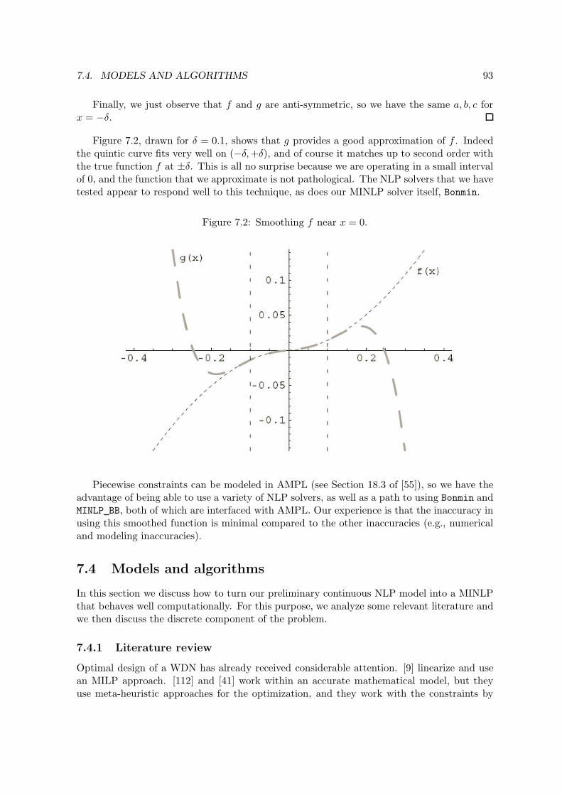
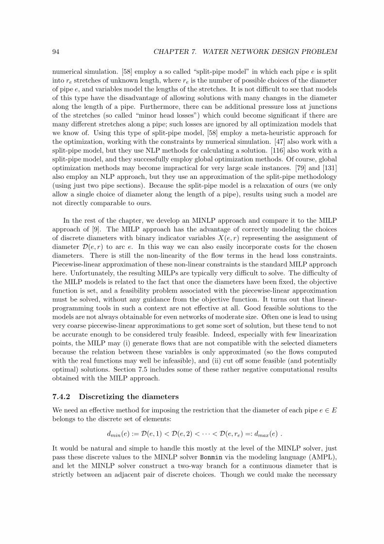
1.1 Example of “unsafe” linearization cut generated from a non-convex constraint 111.2 Linear underestimators before and after branching on continuous variables . . 12

2.1 Outer Approximation constraint cutting off part of the non-convex feasibleregion. . . . . . . . . . . . . . . . . . . . . . . . . . . . . . . . . . . . . . . . . 21

2.2 The convex constraint γ does not cut off x, so nor does any OA linearizationat x. . . . . . . . . . . . . . . . . . . . . . . . . . . . . . . . . . . . . . . . . . 22

3.1 A piecewise-defined univariate function . . . . . . . . . . . . . . . . . . . . . . 343.2 A piecewise-convex lower approximation . . . . . . . . . . . . . . . . . . . . . 343.3 An improved piecewise-convex lower approximation . . . . . . . . . . . . . . . 353.4 The convex relaxation . . . . . . . . . . . . . . . . . . . . . . . . . . . . . . . 373.5 The algorithmic framework . . . . . . . . . . . . . . . . . . . . . . . . . . . . 393.6 UFL: how −gkt(wkt) looks like in the three instances. . . . . . . . . . . . . . . 41

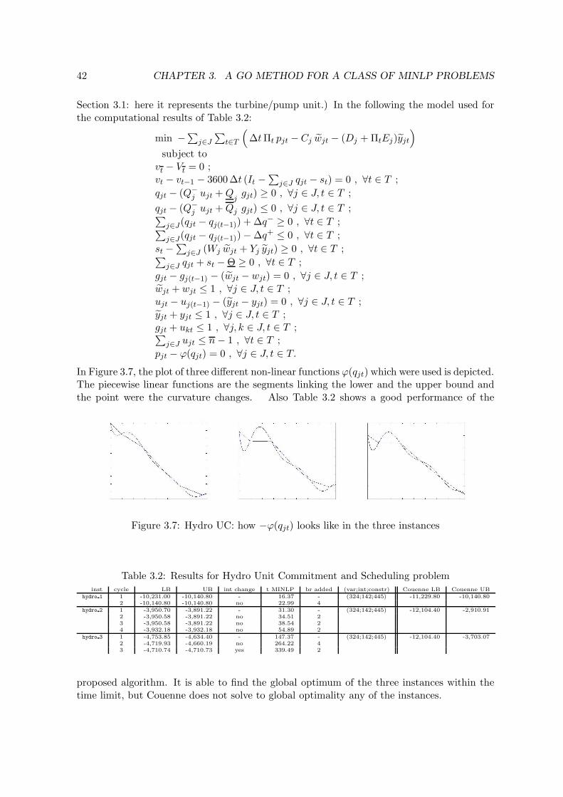
3.7 Hydro UC: how −ϕ(qjt) looks like in the three instances . . . . . . . . . . . . 42

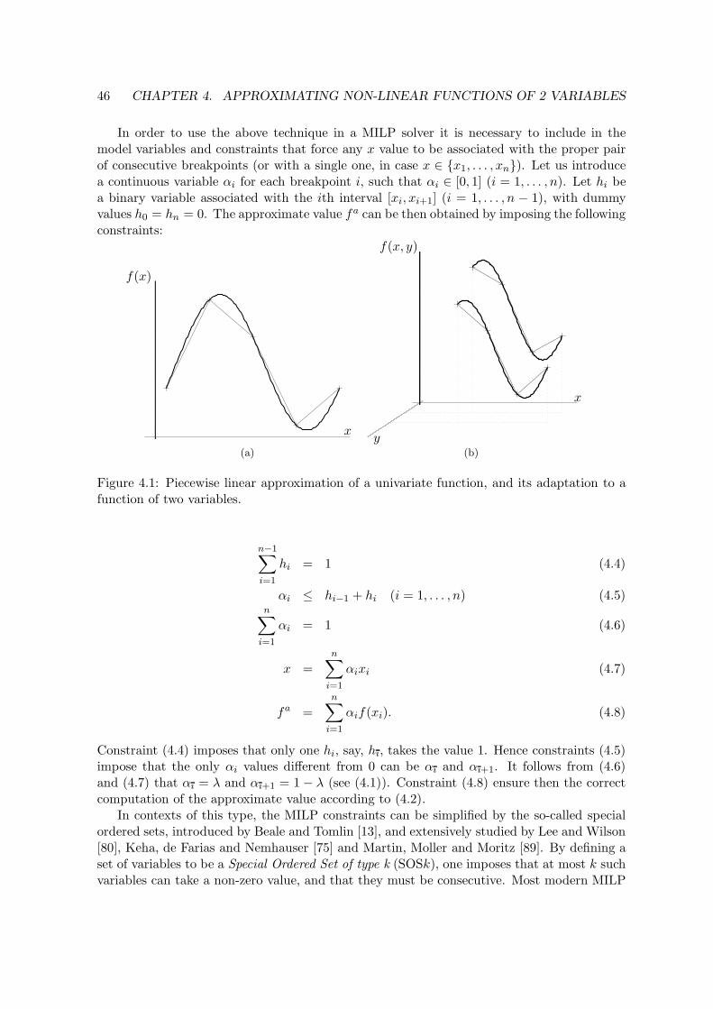
4.1 Piecewise linear approximation of a univariate function, and its adaptation toa function of two variables. . . . . . . . . . . . . . . . . . . . . . . . . . . . . 46

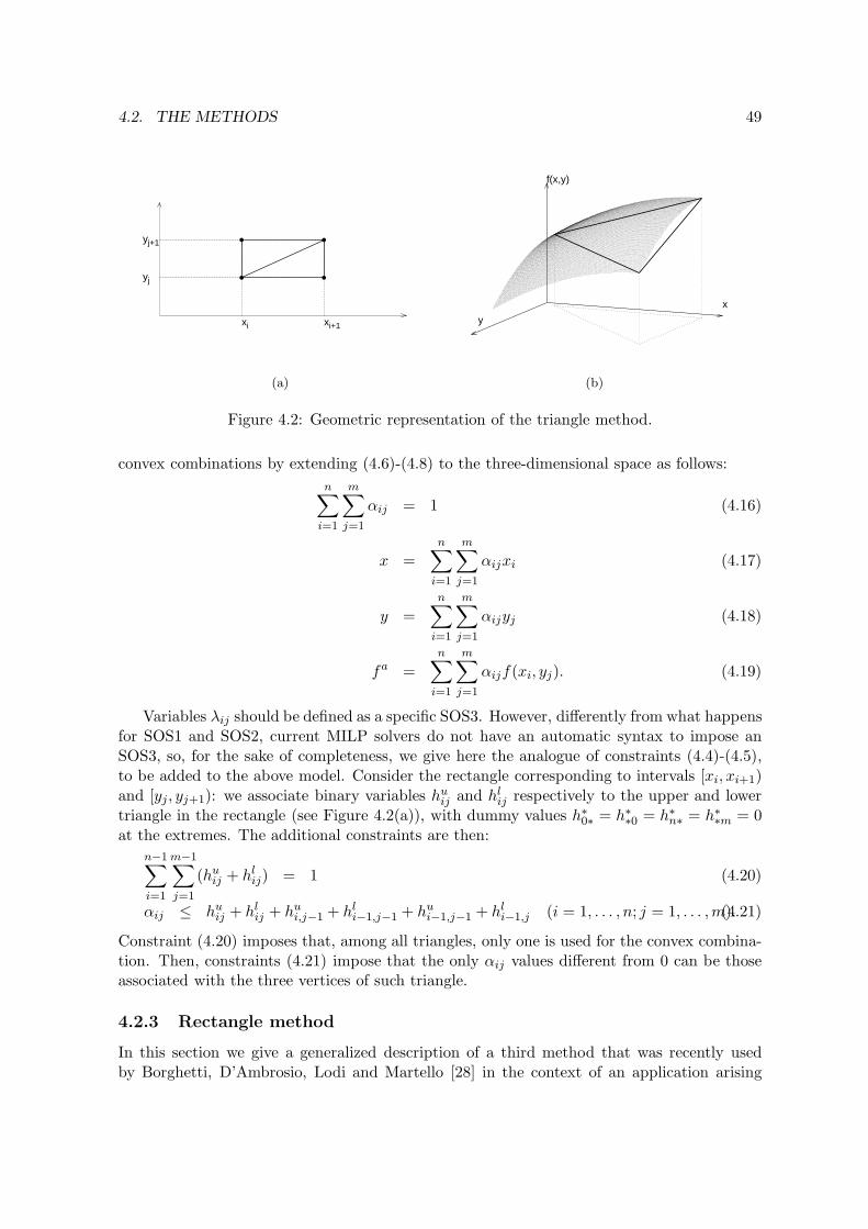
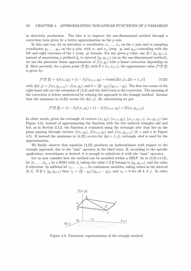
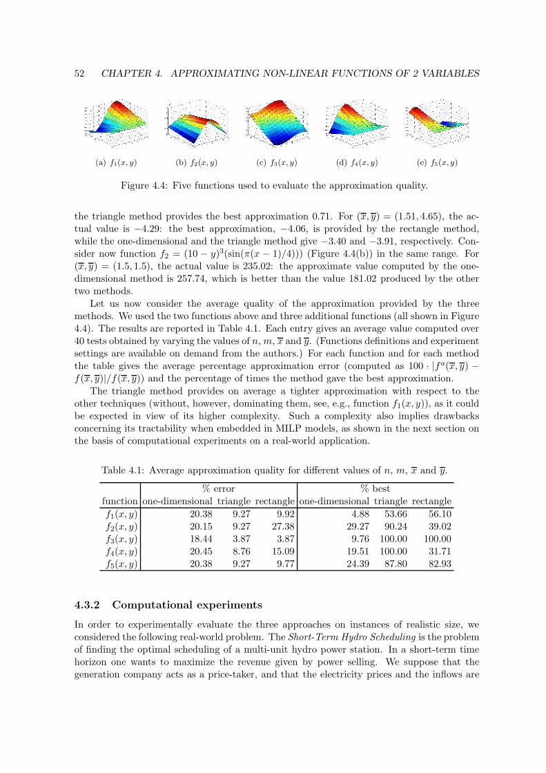
4.2 Geometric representation of the triangle method. . . . . . . . . . . . . . . . . 494.3 Geometric representation of the triangle method. . . . . . . . . . . . . . . . . 504.4 Five functions used to evaluate the approximation quality. . . . . . . . . . . 52

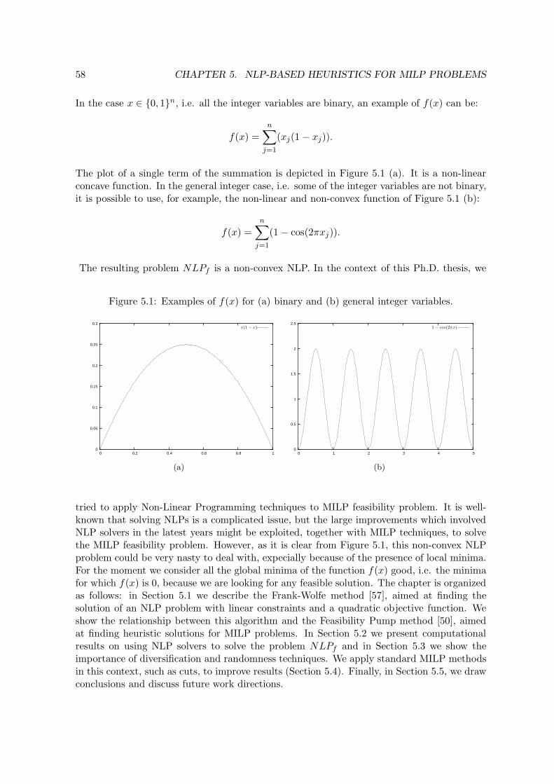
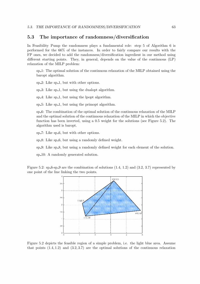
5.1 Examples of f(x) for (a) binary and (b) general integer variables. . . . . . . . 585.2 sp 6-sp 9 are the combination of solutions (1.4, 1.2) and (3.2, 3.7) represented

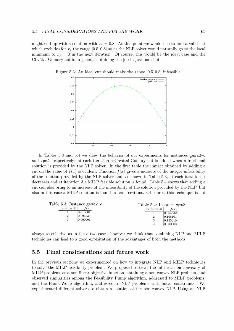
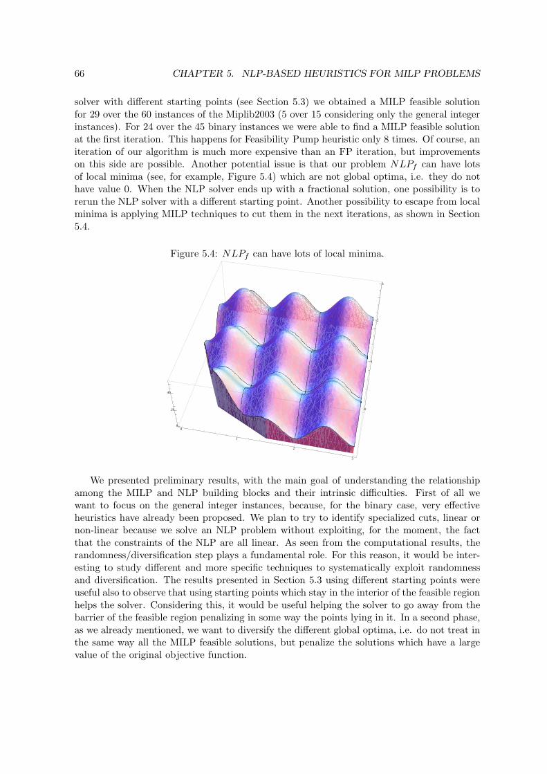
by one point of the line linking the two points. . . . . . . . . . . . . . . . . . 635.3 An ideal cut should make the range [0.5, 0.8] infeasible. . . . . . . . . . . . . . 655.4 NLPf can have lots of local minima. . . . . . . . . . . . . . . . . . . . . . . . 66

6.1 The simple approximation . . . . . . . . . . . . . . . . . . . . . . . . . . . . . 746.2 The enhanced approximation . . . . . . . . . . . . . . . . . . . . . . . . . . . 776.3 Piecewise approximation of the relationship (6.19) for three volume values . . 796.4 Water volumes . . . . . . . . . . . . . . . . . . . . . . . . . . . . . . . . . . . 836.5 Inflow and flows . . . . . . . . . . . . . . . . . . . . . . . . . . . . . . . . . . 856.6 Price and powers . . . . . . . . . . . . . . . . . . . . . . . . . . . . . . . . . . 856.7 Profit . . . . . . . . . . . . . . . . . . . . . . . . . . . . . . . . . . . . . . . . 86

7.1 Three polynomials of different degree approximating the cost function for in-stance foss poly 0, see Section 7.5.1. . . . . . . . . . . . . . . . . . . . . . . 91

ix

x LIST OF FIGURES

7.2 Smoothing f near x = 0. . . . . . . . . . . . . . . . . . . . . . . . . . . . . . . 937.3 Solution for Fossolo network, version foss iron. . . . . . . . . . . . . . . . . 104

List of Tables

2.1 Instances for which a feasible solution was found within the time limit . . . . 282.2 Instances for which the feasible solution found is also the best-know solution 292.3 Instances for which no feasible solution was found within the time limit . . . 292.4 Instances with problems during the execution . . . . . . . . . . . . . . . . . . 29

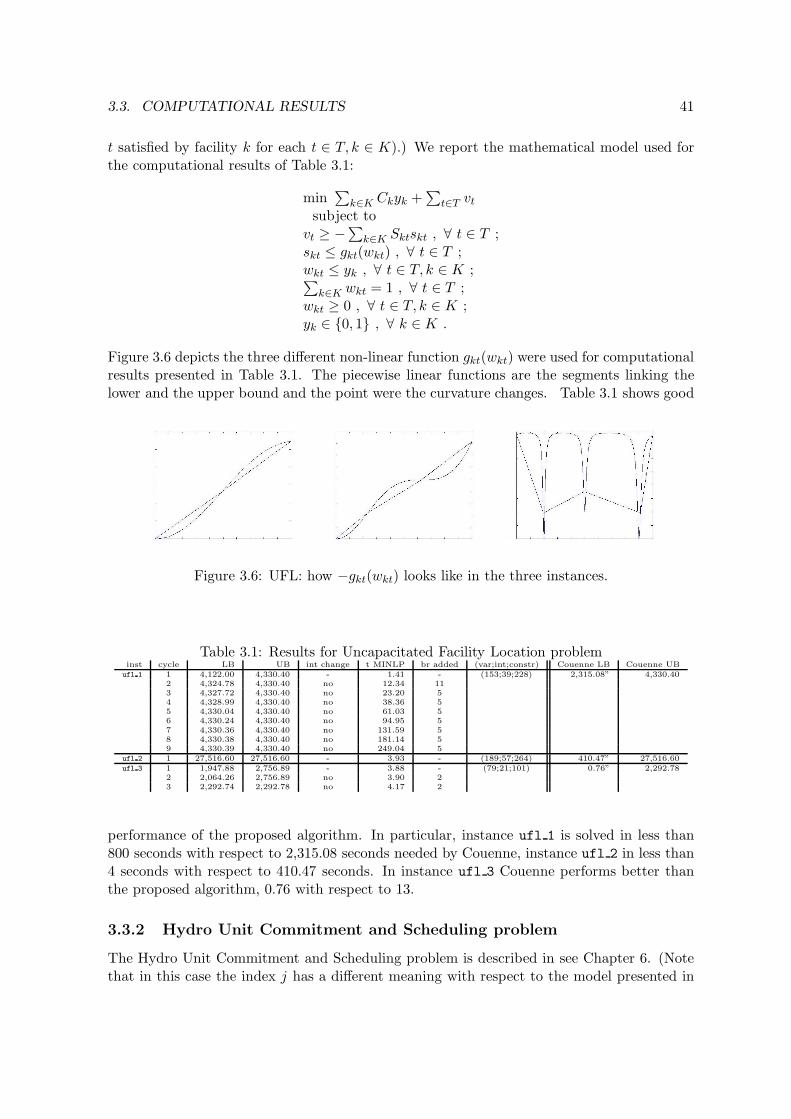
3.1 Results for Uncapacitated Facility Location problem . . . . . . . . . . . . . . 413.2 Results for Hydro Unit Commitment and Scheduling problem . . . . . . . . . 423.3 Results for GLOBALLib and MINLPLib . . . . . . . . . . . . . . . . . . . . . 44

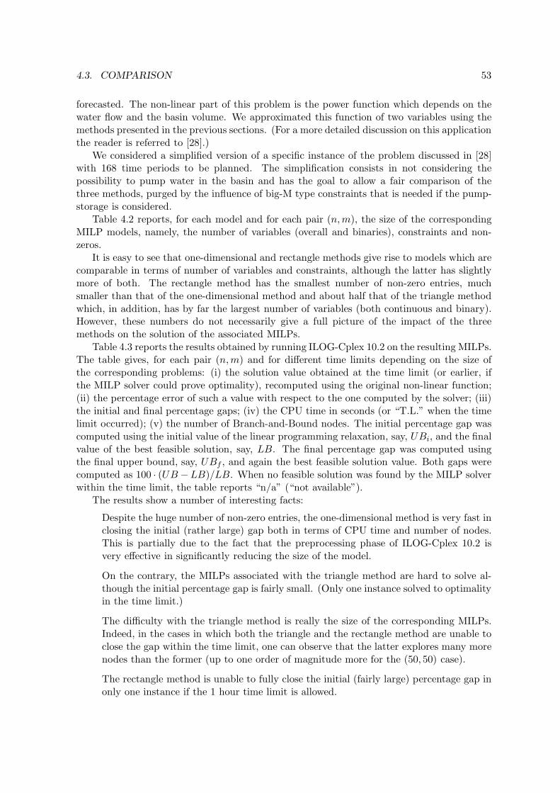
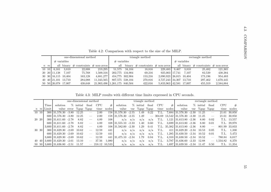
4.1 Average approximation quality for different values of n, m, x and y. . . . . . 524.2 Comparison with respect to the size of the MILP. . . . . . . . . . . . . . . . 554.3 MILP results with different time limits expressed in CPU seconds. . . . . . . 55

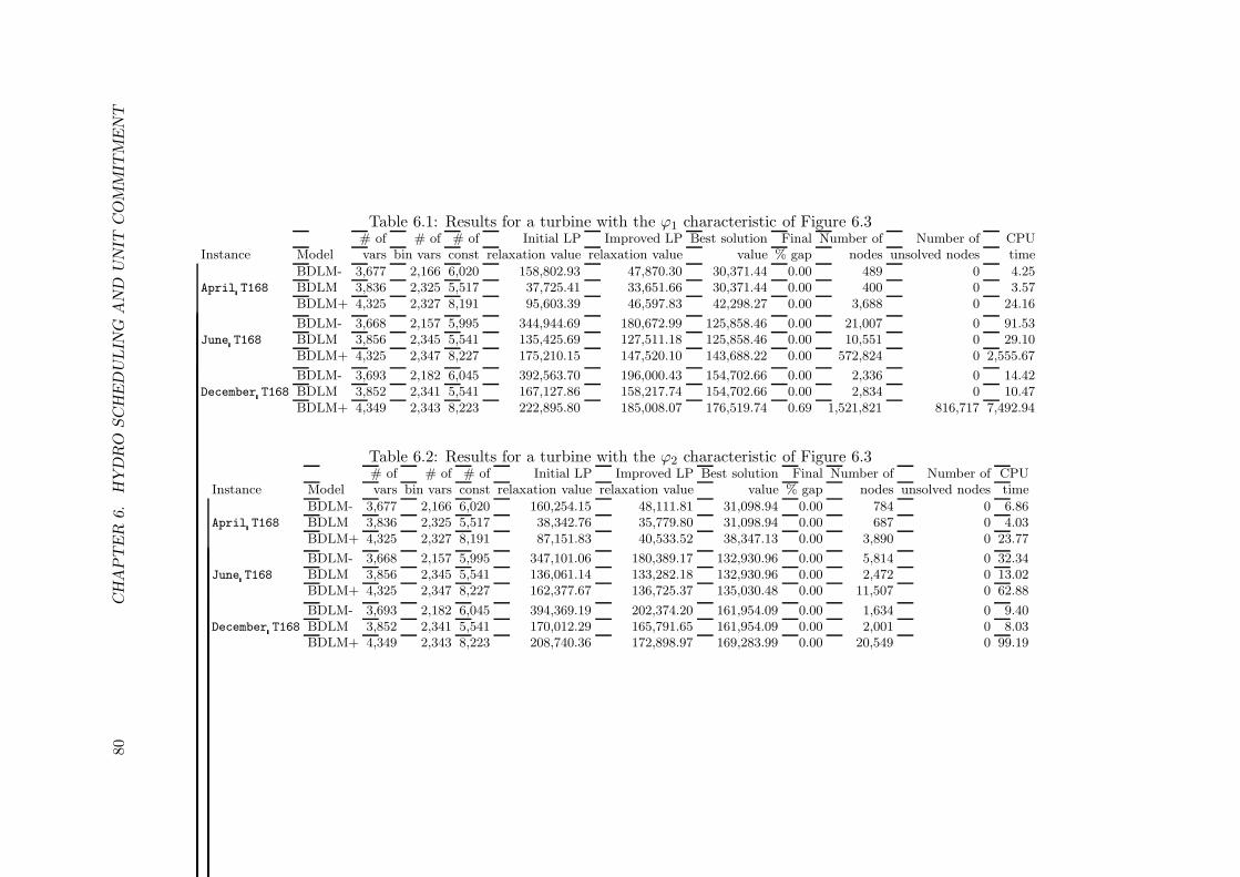
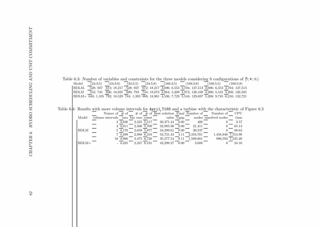
5.1 Comparison among different NLP solvers used for solving problem NLPf . . . 625.2 Results using different starting points. . . . . . . . . . . . . . . . . . . . . . . 645.3 Instance gesa2-o . . . . . . . . . . . . . . . . . . . . . . . . . . . . . . . . . . 655.4 Instance vpm2 . . . . . . . . . . . . . . . . . . . . . . . . . . . . . . . . . . . . 65

6.1 Results for a turbine with the ϕ1 characteristic of Figure 6.3 . . . . . . . . . 806.2 Results for a turbine with the ϕ2 characteristic of Figure 6.3 . . . . . . . . . 806.3 Number of variables and constraints for the three models considering 8 config-

urations of (t; r; z) . . . . . . . . . . . . . . . . . . . . . . . . . . . . . . . . . 826.4 Results with more volume intervals for April T168 and a turbine with the

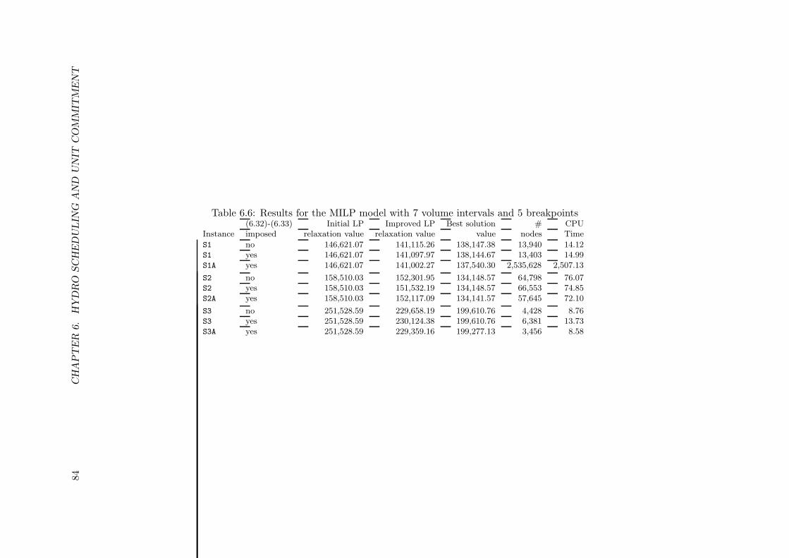
characteristic of Figure 6.3 . . . . . . . . . . . . . . . . . . . . . . . . . . . . . 826.5 Results for BDLM+ with and without the BDLM solution enforced . . . . . . 836.6 Results for the MILP model with 7 volume intervals and 5 breakpoints . . . . 84

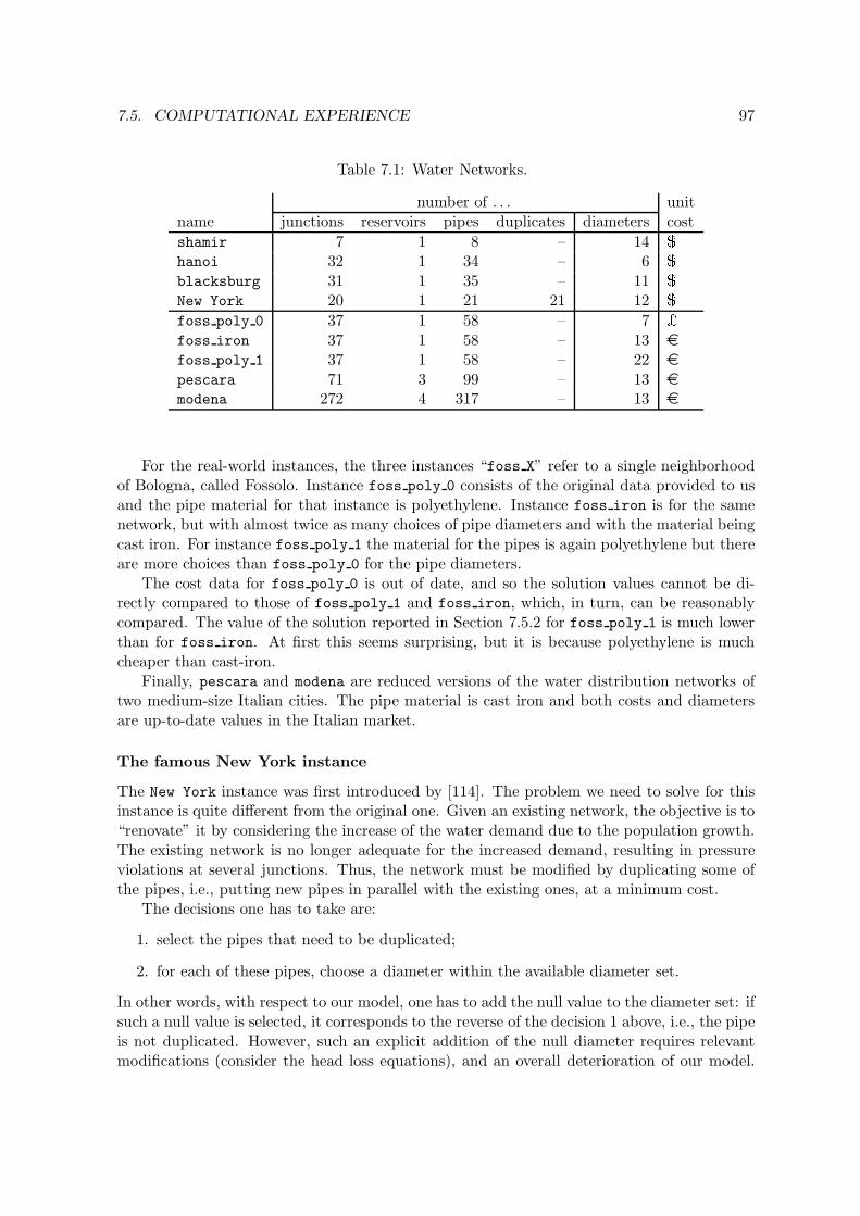
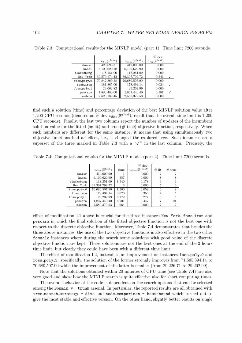
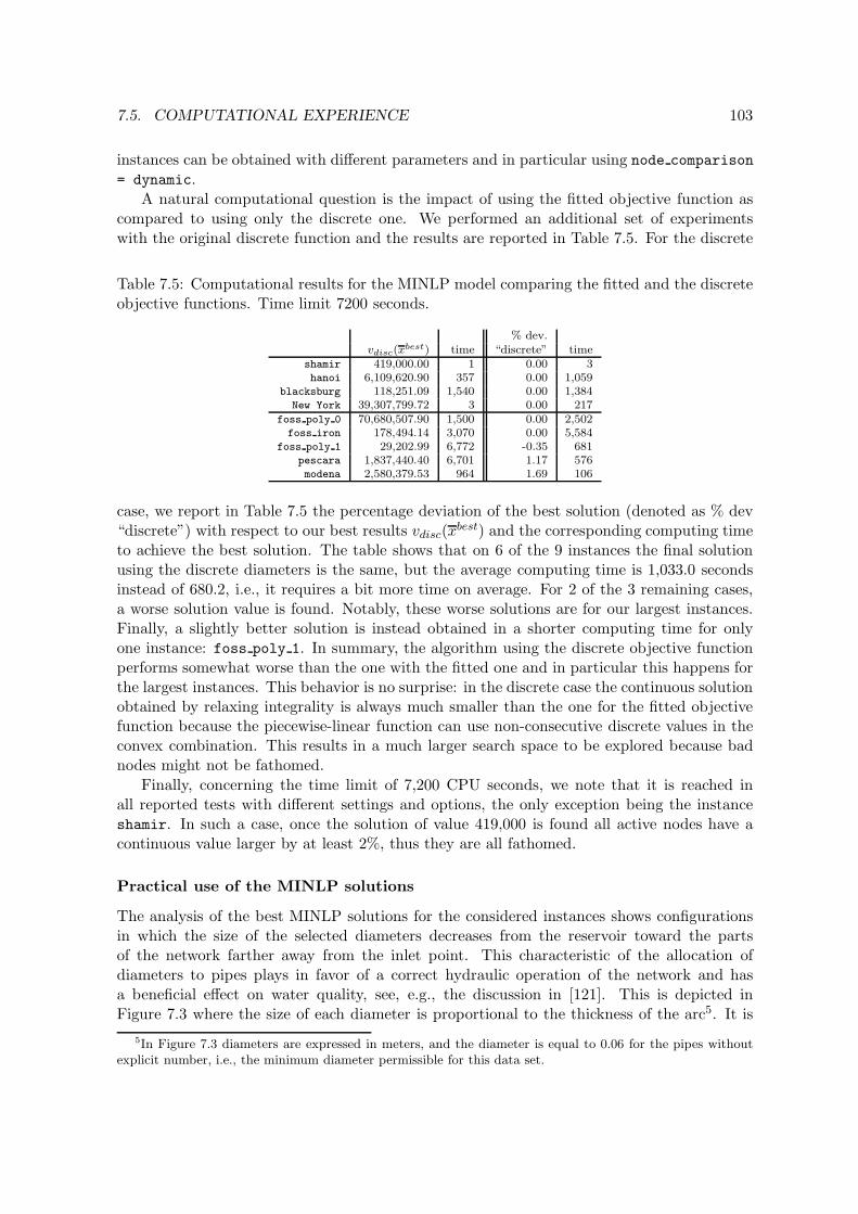
7.1 Water Networks. . . . . . . . . . . . . . . . . . . . . . . . . . . . . . . . . . . 977.2 Characteristics of the 50 continuous solutions at the root node. . . . . . . . 1017.3 Computational results for the MINLP model (part 1). Time limit 7200 seconds.1027.4 Computational results for the MINLP model (part 2). Time limit 7200 seconds. 1027.5 Computational results for the MINLP model comparing the fitted and the

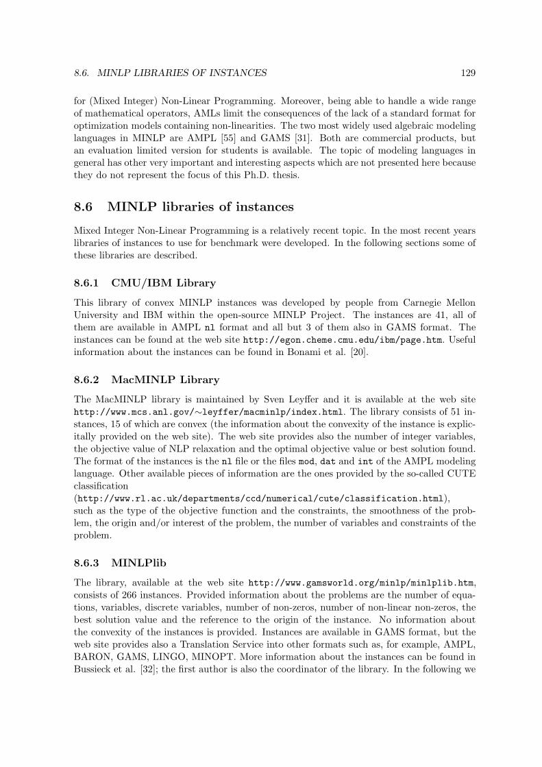
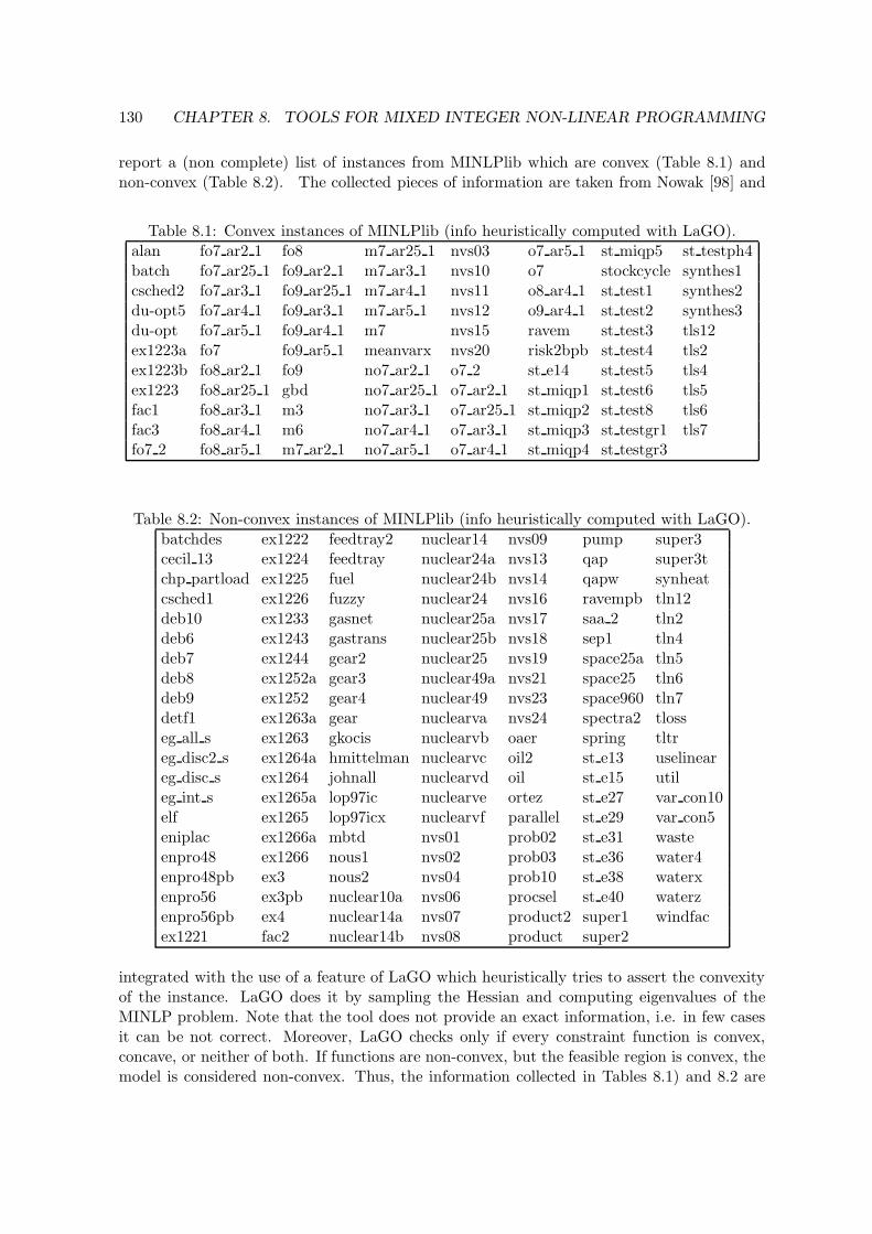
discrete objective functions. Time limit 7200 seconds. . . . . . . . . . . . . . 1037.6 MINLP results compared with literature results. . . . . . . . . . . . . . . . . 106

8.1 Convex instances of MINLPlib (info heuristically computed with LaGO). . . 1308.2 Non-convex instances of MINLPlib (info heuristically computed with LaGO). 130

xi

xii LIST OF TABLES

Preface

In the most recent years there is a renovate interest for Mixed Integer Non-Linear Program-ming (MINLP) problems. This can be explained for different reasons: (i) the performance ofsolvers handling non-linear constraints was largely improved; (ii) the awareness that most ofthe applications from the real-world can be modeled as an MINLP problem; (iii) the challeng-ing nature of this very general class of problems. It is well-known that MINLP problems areNP-hard because they are the generalization of MILP problems, which are NP-hard them-selves. This means that it is very unlikely that a polynomial-time algorithm exists for theseproblems (unless P = NP). However, MINLPs are, in general, also hard to solve in prac-tice. We address to non-convex MINLPs, i.e. having non-convex continuous relaxations: thepresence of non-convexities in the model makes these problems usually even harder to solve.

Until recent years, the standard approach for handling MINLP problems has basicallybeen solving an MILP approximation of it. In particular, linearization of the non-linearconstraints can be applied. The optimal solution of the MILP might be neither optimal norfeasible for the original problem, if no assumptions are done on the MINLPs. Another possibleapproach, if one does not need a proven global optimum, is applying the algorithms tailoredfor convex MINLPs which can be heuristically used for solving non-convex MINLPs. Thethird approach to handle non-convexities is, if possible, to reformulate the problem in orderto obtain a special case of MINLP problems. The exact reformulation can be applied onlyfor limited cases of non-convex MINLPs and allows to obtain an equivalent linear/convexformulation of the non-convex MINLP. The last approach, involving a larger subset of non-convex MINLPs, is based on the use of convex envelopes or underestimators of the non-convexfeasible region. This allows to have a lower bound on the non-convex MINLP optimum thatcan be used within an algorithm like the widely used Branch-and-Bound specialized versionsfor Global Optimization. It is clear that, due to the intrinsic complexity from both practicaland theoretical viewpoint, these algorithms are usually suitable at solving small to mediumsize problems.

The aim of this Ph.D. thesis is to give a flavor of different possible approaches that one canstudy to attack MINLP problems with non-convexities, with a special attention to real-worldproblems. In Part I of the thesis we introduce the problem and present three special cases ofgeneral MINLPs and the most common methods used to solve them. These techniques play afundamental role in the resolution of general MINLP problems. Then we describe algorithmsaddressing general MINLPs. Parts II and III contain the main contributions of the Ph.D.thesis. In particular, in Part II four different methods aimed at solving different classes ofMINLP problems are presented. More precisely:

In Chapter 2 we present a Feasibility Pump (FP) algorithm tailored for non-convexMixed Integer Non-Linear Programming problems. Differences with the previously pro-

xiii

xiv PREFACE

posed FP algorithms and difficulties arising from non-convexities in the models areextensively discussed. We show that the algorithm behaves very well with general prob-lems presenting computational results on instances taken from MINLPLib.

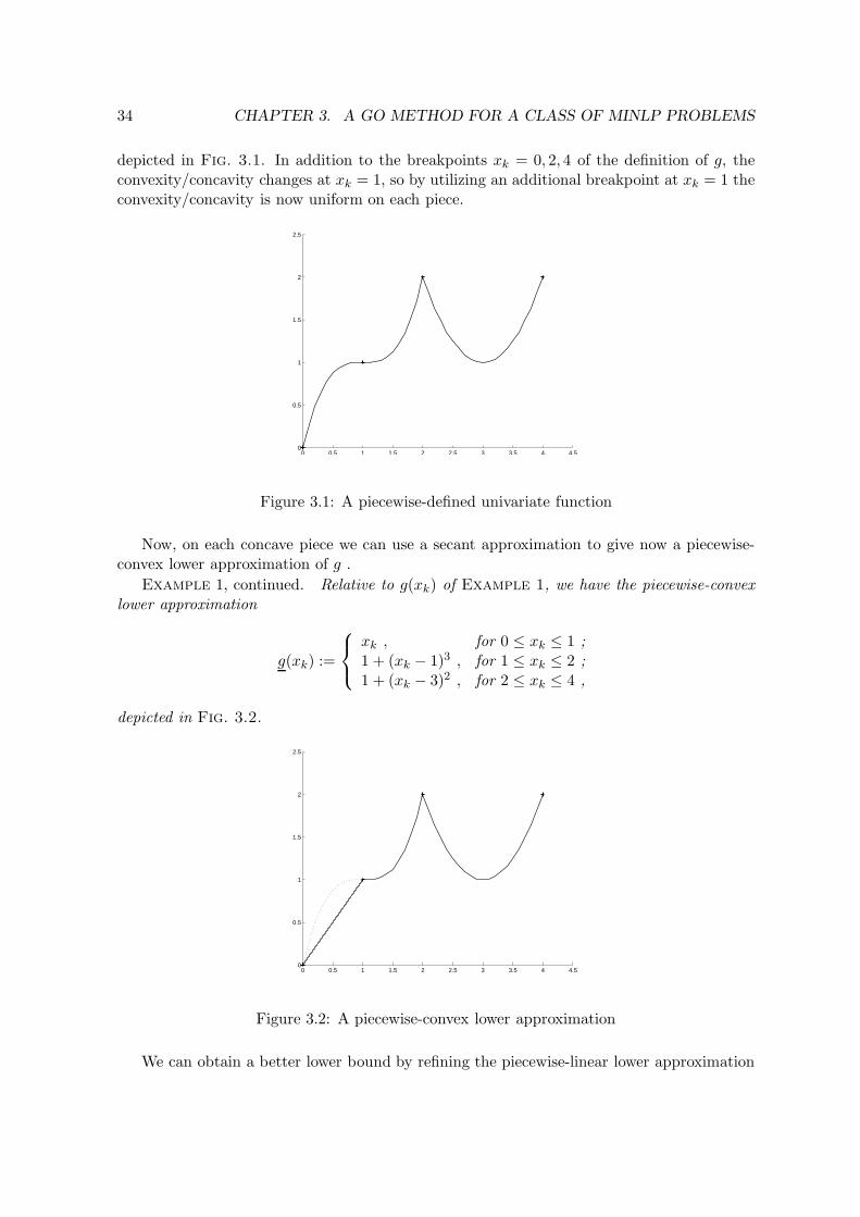
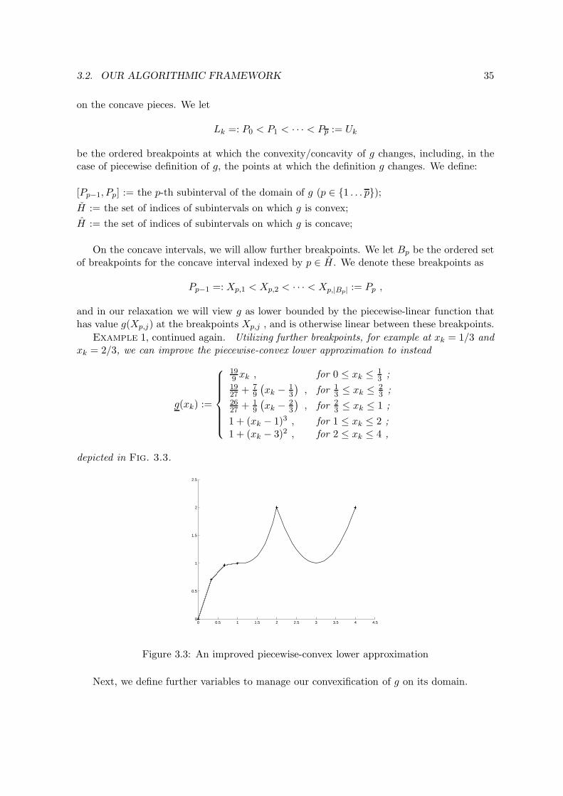
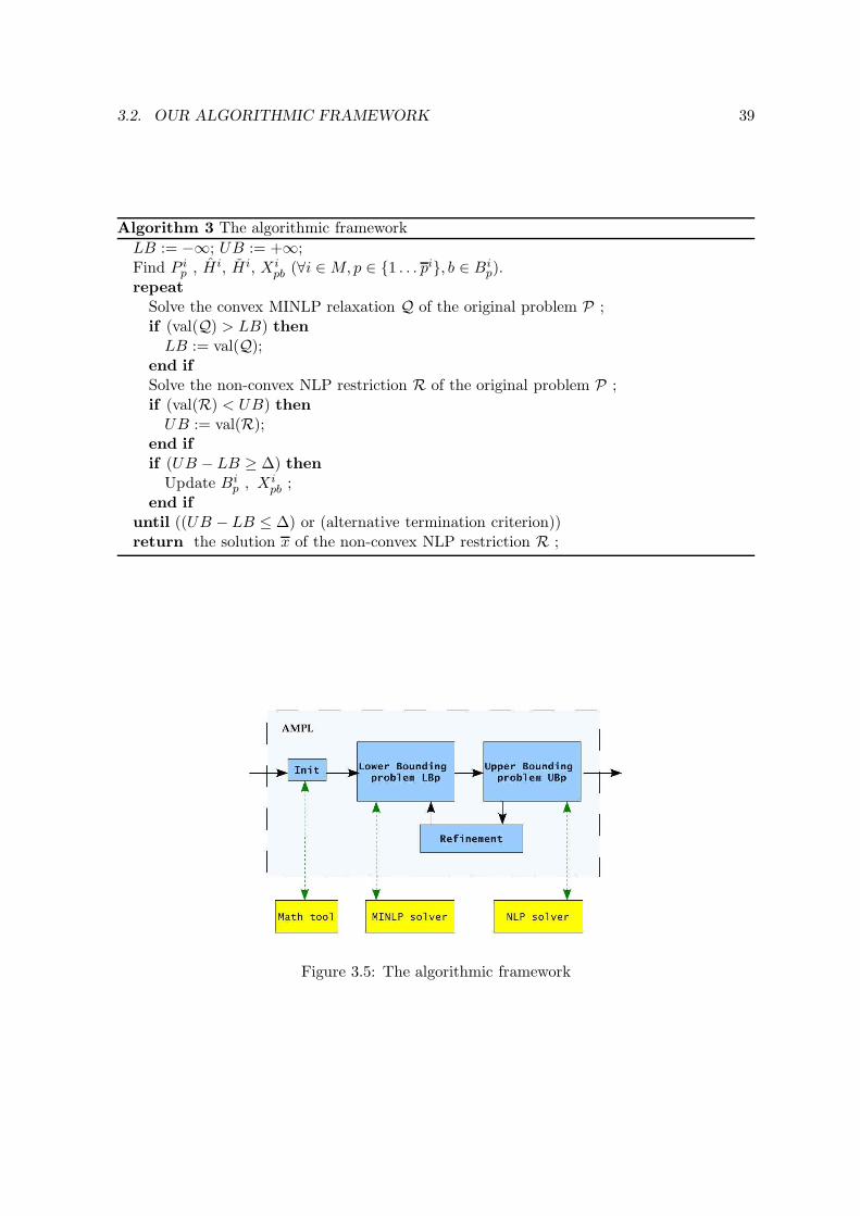
In Chapter 3 we focus on separable non-convex MINLPs, that is where the objectiveand constraint functions are sums of univariate functions. There are many problemsthat are already in such a form, or can be brought into such a form via some simplesubstitutions. We have developed a simple algorithm, implemented at the level of amodeling language (in our case AMPL), to attack such separable problems. First,we identify subintervals of convexity and concavity for the univariate functions usingexternal calls to MATLAB. With such an identification at hand, we develop a convexMINLP relaxation of the problem. We work on each subinterval of convexity andconcavity separately, using linear relaxation on only the “concave side” of each functionon the subintervals. The subintervals are glued together using binary variables. Next,we repeatedly refine our convex MINLP relaxation by modifying it at the modelinglevel. Next, by fixing the integer variables in the original non-convex MINLP, and thenlocally solving the associated non-convex NLP relaxation, we get an upper bound onthe global minimum. We present preliminary computational experiments on differentinstances.

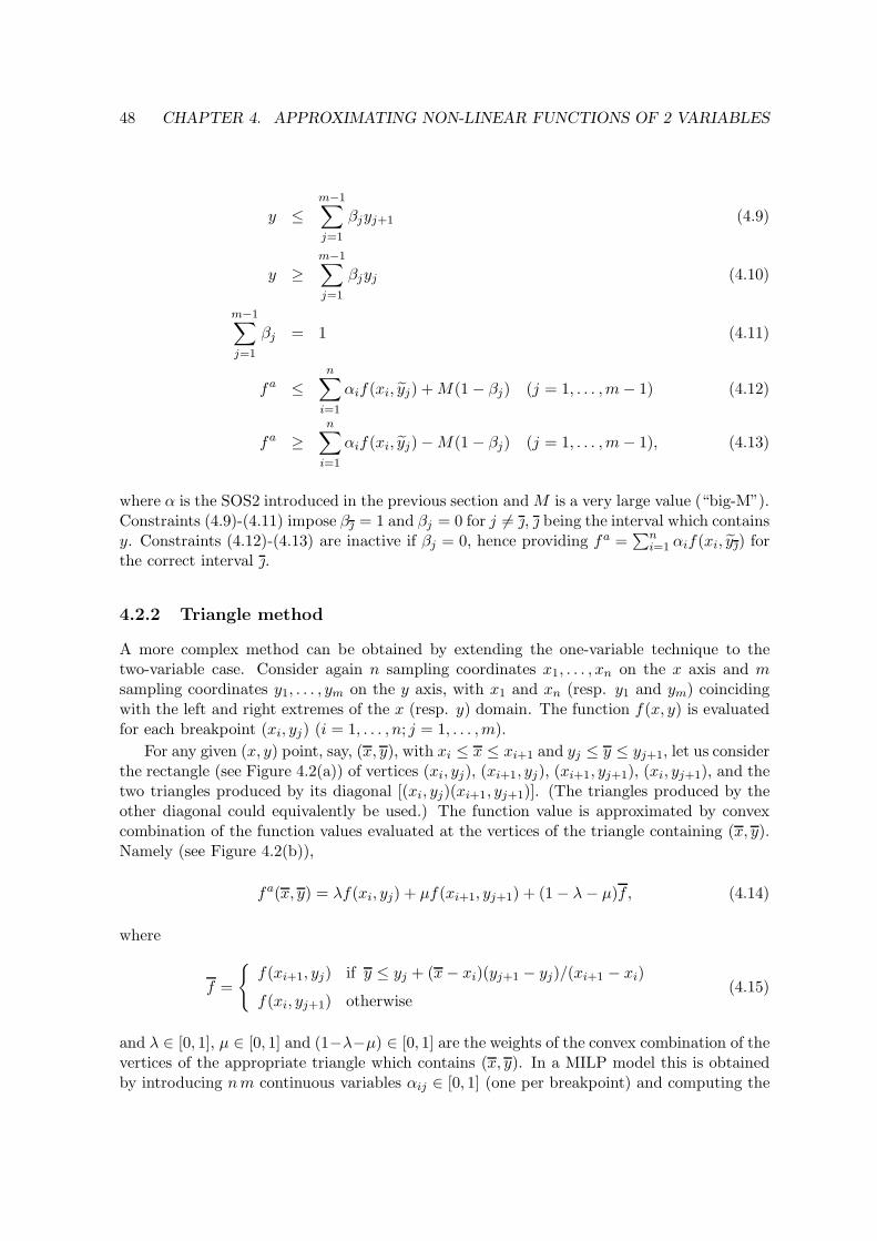
In Chapter 4 we consider three methods for the piecewise linear approximation offunctions of two variables for inclusion within MILP models. The simplest one appliesthe classical one-variable technique over a discretized set of values of the second inde-pendent variable. A more complex approach is based on the definition of triangles in thethree-dimensional space. The third method we describe can be seen as an intermediateapproach, recently used within an applied context, which appears particularly suitablefor MILP modeling. We show that the three approaches do not dominate each other,and give a detailed description of how they can be embedded in a MILP model. Advan-tages and drawbacks of the three methods are discussed on the basis of some numericalexamples.

In Chapter 5 we present preliminary computational results on heuristics for MixedInteger Linear Programming. A heuristic for hard MILP problems based on NLP tech-niques is presented: the peculiarity of our approach to MILP problems is that we re-formulate integrality requirements treating them in the non-convex objective function,ending up with a mapping from the MILP feasibility problem to NLP problem(s). Foreach of these methods, the basic idea and computational results are presented.

Part III of the thesis is devoted to real-world applications: two different problems and ap-proaches to MINLPs are presented, namely Scheduling and Unit Commitment for Hydro-Plants and Water Network Design problems. The results show that each of these differentmethods has advantages and disadvantages. Thus, typically the method to be adopted tosolve a real-world problem should be tailored on the characteristics, structure and size of theproblem. In particular:

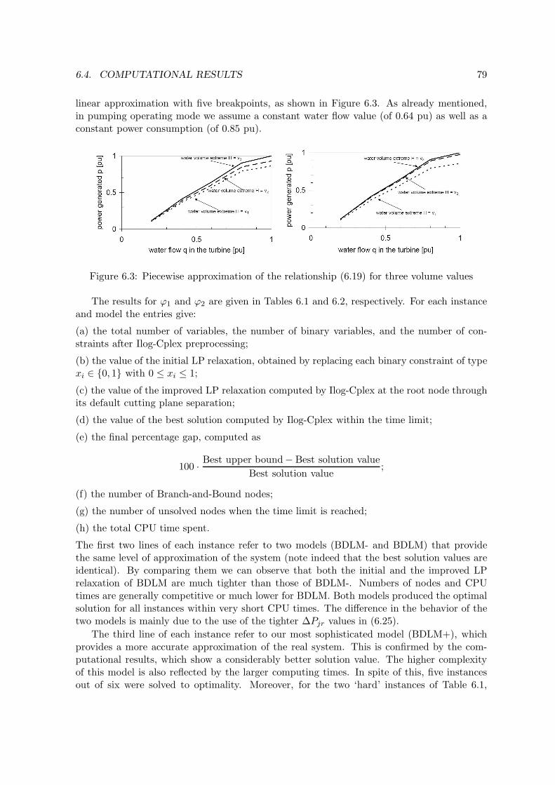
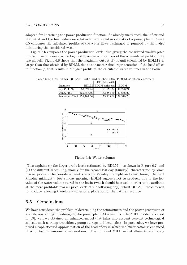
Chapter 6 deals with a unit commitment problem of a generation company whose aimis to find the optimal scheduling of a multi-unit pump-storage hydro power station, fora short term period in which the electricity prices are forecasted. The problem has amixed-integer non-linear structure, that makes very hard to handle the corresponding

xv

mathematical models. However, modern MILP software tools have reached a high ef-ficiency, both in terms of solution accuracy and computing time. Hence we introduceMILP models of increasing complexity, that allow to accurately represent most of thehydro-electric system characteristics, and turn out to be computationally solvable. Inparticular, we present a model that takes into account the head effects on power pro-duction through an enhanced linearization technique, and turns out to be more generaland efficient than those available in the literature. The practical behavior of the modelsis analyzed through computational experiments on real-world data.

In Chapter 7 we present a solution method for a water-network optimization problemusing a non-convex continuous NLP relaxation and a MINLP search. Our approachemploys a relatively simple and accurate model that pays some attention to the re-quirements of the solvers that we employ. Our view is that in doing so, with the goalof calculating only good feasible solutions, complicated algorithmics can be confinedto the MINLP solver. We report successful computational experience using availableopen-source MINLP software on problems from the literature and on difficult real-worldinstances.

Part IV of the thesis consists of a brief review on tools commonly used for general MINLPproblems. We present the main characteristics of solvers for each special case of MINLP.Then we present solvers for general MINLPs: for each solver a brief description, taken fromthe manuals, is given together with a schematic table containing the most importart piecesof information, for example, the class of problems they address, the algorithms implemented,the dependencies with external software.

Tools for MINLP, especially open-source software, constituted an integral part of thedevelopment of this Ph.D. thesis. Also for this reason Part IV is devoted to this topic.Methods presented in Chapters 4, 5 and 7 were completely developed using open-source solvers(and partially Chapter 3). A notable example of the importance of open-source solvers is givenin Chapter 7: we present an algorithm for solving a non-convex MINLP problem, namely theWater Network Design problem, using the open-source software Bonmin. The solver wasoriginally tailored for convex MINLPs. However, some accommodations were made to handlenon-convex problems and they were developed and tested in the context of the work presentedin Chapter 7, where details on these features can be found.

xvi PREFACE

Part I

Introduction

1

Chapter 1

Introduction to Mixed IntegerNon-Linear Programming Problemsand Methods

The (general) Mixed Integer Non-Linear Programming (MINLP) problem which we are in-terested in has the following form:

MINLP

min f(x, y) (1.1)

g(x, y) ≤ 0 (1.2)

x ∈ X ∩ Zn (1.3)

y ∈ Y , (1.4)

where f : Rn×p → R, g : R

n×p → Rm, X and Y are two polyhedra of appropriate dimension

(including bounds on the variables). We assume that f and g are twice continuously differ-entiable, but we do not make any other assumption on the characteristics of these functionsor their convexity/concavity. In the following, we will call problems of this type non-convexMixed Integer Non-Linear Programming problems.

Non-convex MINLP problems are NP-hard because they generalize MILP problems whichare NP-hard themselves (for a detailed discussion on the complexity of MILPs we refer thereader to Garey and Johnson [61]).

The most complex aspect we need to have in mind when we work with non-convex MINLPsis that its continuous relaxation, i.e. the problem obtained by relaxing the integrality require-ment on the x variables, might have (and usually it has) local optima, i.e. solutions whichare optimal within a restricted part of the feasible region (neighborhood), but not consideringthe entire feasible region. This does not happen when f and g are convex (or linear): in thesecases the local optima are also global optima, i.e. solutions which are optimal considering theentire feasible region.

To understand more in detail the issue, let us consider the continuous relaxation of theMINLP problem. The first order optimality conditions are necessary, but, only when f andg are convex, they are also sufficient for the stationary point (x, y) which satisfies them to be

3

4 CHAPTER 1. INTRODUCTION TO MINLP PROBLEMS AND METHODS

the global optimum:

g(x, y) ≤ 0 (1.5)

x ∈ X (1.6)

y ∈ Y (1.7)

λ ≥ 0 (1.8)

∇f(x, y) +

m∑

i=1

λi∇gi(x, y) = 0 (1.9)

λT g(x, y) = 0, (1.10)

where ∇ is the Jacobian of the function and λ are the dual variables, i.e. the variables of theDual problem of the continuous relaxation of MINLP which is called Primal problem. TheDual problem is formalized as follows:

maxλ≥0

[infx∈X,y∈Y f(x, y) + λT g(x, y)], (1.11)

see [17, 97] for details on Duality Theory in NLP. Equations (1.5)-(1.7) are the primal feasibil-ity conditions, equation (1.8) is the dual feasibility condition, equation (1.9) is the stationaritycondition and equation (1.10) is the complementarity condition.

These conditions, called also Karush-Kuhn-Tucker (KKT) conditions, assume an impor-tant role in algorithms we will present and use in this Ph.D. thesis. For details the reader isreferred to Karush [74], Kuhn and Tucker [77].

The aim of this Ph.D. thesis is presenting methods for solving non-convex MINLPs andmodels for real-world applications of this type. However, in the remaining part of this sec-tion, we will present special cases of general MINLP problems because they play an importantrole in the resolution of the more general problem. Though, this introduction will not coverexhaustively topics concerning Mixed Integer Linear Programming (MILP), Non-Linear Pro-gramming (NLP) and Mixed Integer Non-Linear Programming in general, but only give aflavor of the ingredients necessary to fully understand the methods and algorithms which arethe contribution of the thesis. For each problem, references will be provided to the interestedreader.

1.1 Mixed Integer Linear Programming

A Mixed Integer Linear Programming problem is the special case of the MINLP problem inwhich functions f and g assume a linear form. It is usually written in the form:

MILPmin cT x + dT y

Ax + By ≤ b

x ∈ X ∩ Zn

y ∈ Y,

where A and B are, respectively, the m × n and the m × p matrices of coefficients, b is them-dimensional vector, called right-hand side, c and d are, respectively, the n-dimensional and

1.1. MIXED INTEGER LINEAR PROGRAMMING 5

the p-dimensional vectors of costs. Even if these problems are a special and, in general, easiercase with respect to MINLPs, they are NP-hard (see Garey and Johnson [61]). This meansthat a polynomial algorithm to solve MILP is unlikely to exists, unless P = NP.

Different possible approaches to this problem have been proposed. The most effective onesand extensively used in the modern solvers are Branch-and-Bound (see Land and Doig [78]),cutting planes (see Gomory [64]) and Branch-and-Cut (see Padberg and Rinaldi [102]). Theseare exact methods: this means that, if an optimal solution for the MILP problem exists, theyfind it. Otherwise, they prove that such a solution does not exist. In the following we give abrief description of the main ideas of these methods, which, as we will see, are the basis forthe algorithms proposed for general MINLPs.

Branch-and-Bound (BB): the first step is solving the continuous relaxation of MILP(i.e. the problem obtained relaxing the integrality constraints on the x variables, LP ={min cT x+ dT y | Ax+By ≤ b, x ∈ X, y ∈ Y }). Then, given a fractional value x∗

j fromthe solution of LP (x∗, y∗), the problem is divided into two subproblems, the first wherethe constraint xj ≤ ⌊x∗

j⌋ is added and the second where the constraint xj ≥ ⌊x∗j⌋ + 1

is added. Each of these new constraints represents a “branching decision” because thepartition of the problem in subproblems is represented with a tree structure, the BBtree. Each subproblem is represented as a node of the BB tree and, from a mathematicalviewpoint, has the form:

LP min cT x + dT y

Ax + By ≤ b

x ∈ X

y ∈ Y

x ≤ lk

x ≥ uk,

where lk and uk are vectors defined so as to mathematically represent the branchingdecisions taken so far in the previous levels of the BB tree. The process is iterated foreach node until the solution of the continuous relaxation of the subproblem is integerfeasible or the continuous relaxation is infeasible or the lower bound value of subprob-lem is not smaller than the current incumbent solution, i.e. the best feasible solutionencountered so far. In these three cases, the node is fathomed. The algorithm stopswhen no node to explore is left, returning the best solution found so far which is provento be optimal.

Cutting Plane (CP): as in the Branch-and-Bound method, the LP relaxation is solved.Given the fractional LP solution (x∗, y∗), a separation problem is solved, i.e. a problemwhose aim is finding a valid linear inequality that cuts off (x∗, y∗), i.e. it is not satisfiedby (x∗, y∗). An inequality is valid for the MILP problem if it is satisfied by any integerfeasible solution of the problem. Once a valid inequality (cut) is found, it is added to theproblem: it makes the LP relaxation tighter and the iterative addition of cuts might leadto an integer solution. Different types of cuts have been studied, for example, Gomorymixed integer cuts, Chvatal-Gomory cuts, mixed integer rounding cuts, rounding cuts,lift-and-project cuts, split cuts, clique cuts (see [40]). Their effectiveness depends onthe MILP problem and usually different types of cuts are combined.


Branch-and-Cut (BC): the idea is integrating the two methods described above, merg-ing the advantages of both techniques. Like in BB, at the root node the LP relaxationis solved. If the solution is not integer feasible, a separation problem is solved and, inthe case cuts are fonud, they are added to the problem, otherwise a branching decisionis performed. This happens also to non-leaf nodes, the LP relaxation correspondent tothe node is solved, a separation problem is computed and cuts are added or branch isperformed. This method is very effective and, like in CP, different types of cuts can beused.

An important part of the modern solvers, usually integrated with the exact methods, areheuristic methods: their aim is finding rapidly a “good” feasible solution or improving thebest solution found so far. No guarantee on the optimality of the solution found is given.Examples of the first class of heuristics are: simple rounding heuristics, Feasibility Pump(see Fischetti et al. [50], Bertacco et al. [16], Achterberg and Berthold [3]). Examples ofthe second class of heuristics are metaheuristics (see, for example, Glover and Kochenberger[63]), Relaxation Induced Neighborhoods Search (see Danna et al. [43]) and Local Branching(see Fischetti and Lodi [51]).

For a survey of the methods and the development of the software addressed at solvingMILPs the reader is referred to the recent paper by Lodi [87], and for a detailed discussionsee [2, 18, 19, 66, 95, 104].

1.2 Non-Linear Programming

Another special case of MINLP problems is Non-Linear Programming: the functions f and gare non-linear but n = 0, i.e. no variable is required to be integer. The classical NLP problemcan be written in the following form:

NLPmin f(y) (1.12)

g(y) ≤ 0 (1.13)

y ∈ Y. (1.14)

Different issues arise when one tries to solve this kind of problems. Some heuristic andexact methods are tailored for a widely studied subclass of these problems: convex NLPs.In this case, the additional assumption is that f and g are convex functions. Some of thesemethods can be used for more general non-convex NLPs, but no guarantee on the globaloptimality of the solution is given. In particular, when no assumption on convexity is done,the problem usually has local optimal solutions. In the non-convex case, exact algorithms, i.e.those methods that are guaranteed to find the global solution, are called Global Optimizationmethods.

In the following we sketch some of the most effective algorithms studied and actuallyimplemented within available NLP solvers (see Section 8):

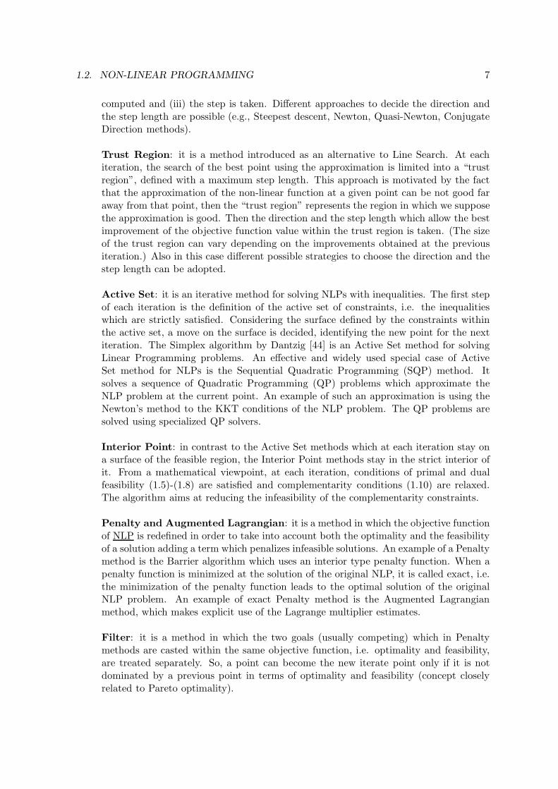
Line Search: introduced for unconstrained optimization problems with non-linear ob-jective function, it is an iterative method used also as part of methods for constrainedNLPs. At each iteration an approximation of the non-linear function is considered and(i) a search direction is decided; (ii) the step length to take along that direction is

1.2. NON-LINEAR PROGRAMMING 7

computed and (iii) the step is taken. Different approaches to decide the direction andthe step length are possible (e.g., Steepest descent, Newton, Quasi-Newton, ConjugateDirection methods).

Trust Region: it is a method introduced as an alternative to Line Search. At eachiteration, the search of the best point using the approximation is limited into a “trustregion”, defined with a maximum step length. This approach is motivated by the factthat the approximation of the non-linear function at a given point can be not good faraway from that point, then the “trust region” represents the region in which we supposethe approximation is good. Then the direction and the step length which allow the bestimprovement of the objective function value within the trust region is taken. (The sizeof the trust region can vary depending on the improvements obtained at the previousiteration.) Also in this case different possible strategies to choose the direction and thestep length can be adopted.

Active Set: it is an iterative method for solving NLPs with inequalities. The first stepof each iteration is the definition of the active set of constraints, i.e. the inequalitieswhich are strictly satisfied. Considering the surface defined by the constraints withinthe active set, a move on the surface is decided, identifying the new point for the nextiteration. The Simplex algorithm by Dantzig [44] is an Active Set method for solvingLinear Programming problems. An effective and widely used special case of ActiveSet method for NLPs is the Sequential Quadratic Programming (SQP) method. Itsolves a sequence of Quadratic Programming (QP) problems which approximate theNLP problem at the current point. An example of such an approximation is using theNewton’s method to the KKT conditions of the NLP problem. The QP problems aresolved using specialized QP solvers.

Interior Point: in contrast to the Active Set methods which at each iteration stay ona surface of the feasible region, the Interior Point methods stay in the strict interior ofit. From a mathematical viewpoint, at each iteration, conditions of primal and dualfeasibility (1.5)-(1.8) are satisfied and complementarity conditions (1.10) are relaxed.The algorithm aims at reducing the infeasibility of the complementarity constraints.

Penalty and Augmented Lagrangian: it is a method in which the objective functionof NLP is redefined in order to take into account both the optimality and the feasibilityof a solution adding a term which penalizes infeasible solutions. An example of a Penaltymethod is the Barrier algorithm which uses an interior type penalty function. When apenalty function is minimized at the solution of the original NLP, it is called exact, i.e.the minimization of the penalty function leads to the optimal solution of the originalNLP problem. An example of exact Penalty method is the Augmented Lagrangianmethod, which makes explicit use of the Lagrange multiplier estimates.

Filter: it is a method in which the two goals (usually competing) which in Penaltymethods are casted within the same objective function, i.e. optimality and feasibility,are treated separately. So, a point can become the new iterate point only if it is notdominated by a previous point in terms of optimality and feasibility (concept closelyrelated to Pareto optimality).


For details on the algorithms mentioned above and their convergence, the reader is referredto, for example, [12, 17, 29, 54, 97, 105]. In the context of the contribution of this Ph.D. thesis,the NLP methods and solvers are used as black boxed, i.e. selecting them according to theircharacteristics and efficiency with respect to the problem, but without changing them.

1.3 Convex Mixed Integer Non-Linear Programming

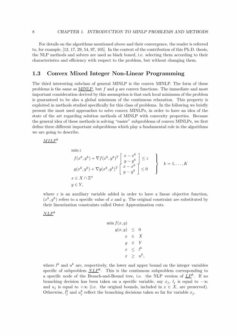
The third interesting subclass of general MINLP is the convex MINLP. The form of theseproblems is the same as MINLP, but f and g are convex functions. The immediate and mostimportant consideration derived by this assumption is that each local minimum of the problemis guaranteed to be also a global minimum of the continuous relaxation. This property isexploited in methods studied specifically for this class of problems. In the following we brieflypresent the most used approaches to solve convex MINLPs, in order to have an idea of thestate of the art regarding solution methods of MINLP with convexity properties. Becausethe general idea of these methods is solving “easier” subproblems of convex MINLPs, we firstdefine three different important subproblems which play a fundamental role in the algorithmswe are going to describe.

MILP k

min z

f(xk, yk) + ∇f(xk, yk)T[

x − xk

y − yk

]≤ z

g(xk, yk) + ∇g(xk, yk)T[

x − xk

y − yk

]≤ 0

k = 1, . . . ,K

x ∈ X ∩ Zn

y ∈ Y,

where z is an auxiliary variable added in order to have a linear objective function,(xk, yk) refers to a specific value of x and y. The original constraint are substituted bytheir linearization constraints called Outer Approximation cuts.

NLP k

min f(x, y)

g(x, y) ≤ 0

x ∈ X

y ∈ Y

x ≤ lk

x ≥ uk,

where lk and uk are, respectively, the lower and upper bound on the integer variablesspecific of subproblem NLP k. This is the continuous subproblem corresponding toa specific node of the Branch-and-Bound tree, i.e. the NLP version of LP k. If nobranching decision has been taken on a specific variable, say xj , lj is equal to −∞and uj is equal to +∞ (i.e. the original bounds, included in x ∈ X, are preserved).Otherwise, lkj and uk

j reflect the branching decisions taken so far for variable xj .

1.3. CONVEX MIXED INTEGER NON-LINEAR PROGRAMMING 9

NLP kx

min f(xk, y)

g(xk, y) ≤ 0

y ∈ Y,

where the integer part of the problem is fixed according to the integer vector xk.

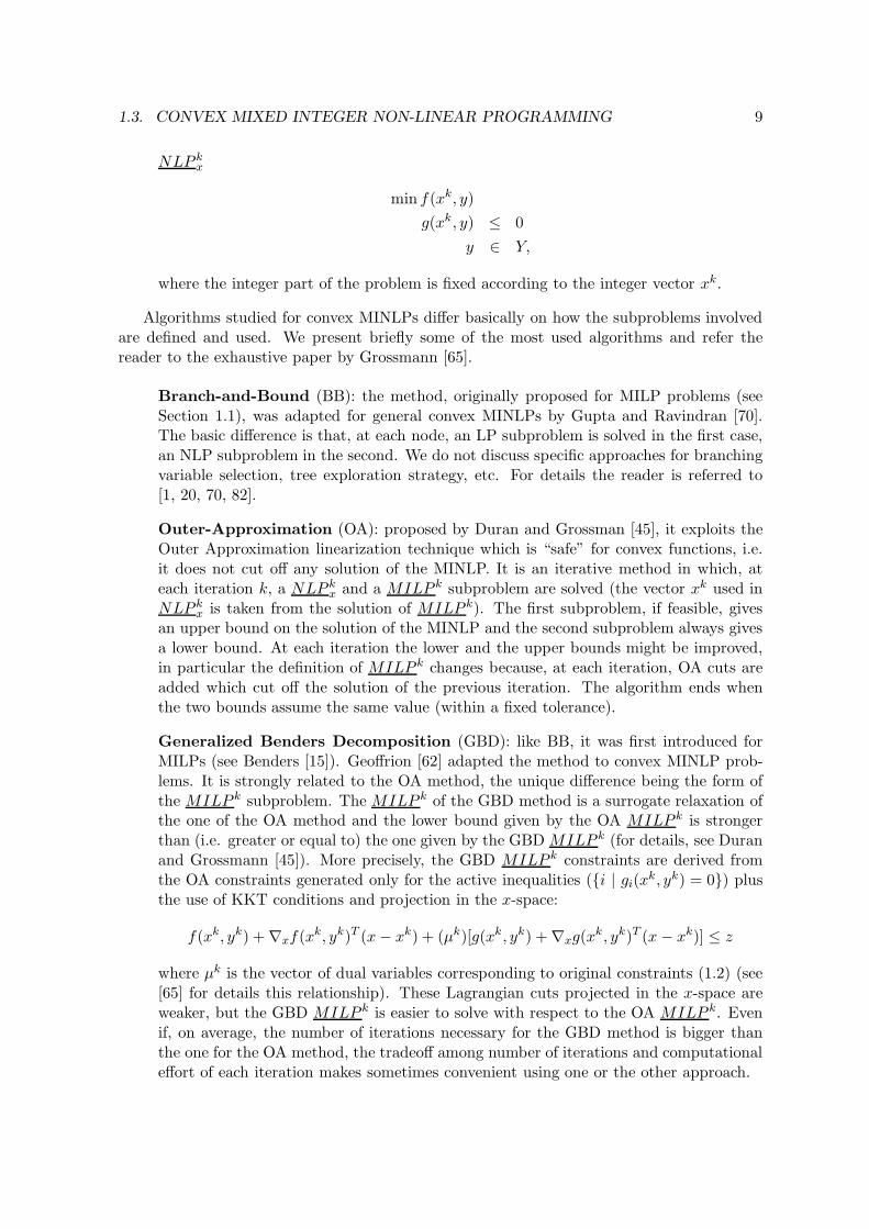
Algorithms studied for convex MINLPs differ basically on how the subproblems involvedare defined and used. We present briefly some of the most used algorithms and refer thereader to the exhaustive paper by Grossmann [65].

Branch-and-Bound (BB): the method, originally proposed for MILP problems (seeSection 1.1), was adapted for general convex MINLPs by Gupta and Ravindran [70].The basic difference is that, at each node, an LP subproblem is solved in the first case,an NLP subproblem in the second. We do not discuss specific approaches for branchingvariable selection, tree exploration strategy, etc. For details the reader is referred to[1, 20, 70, 82].

Outer-Approximation (OA): proposed by Duran and Grossman [45], it exploits theOuter Approximation linearization technique which is “safe” for convex functions, i.e.it does not cut off any solution of the MINLP. It is an iterative method in which, ateach iteration k, a NLP k

x and a MILP k subproblem are solved (the vector xk used inNLP k

x is taken from the solution of MILP k). The first subproblem, if feasible, givesan upper bound on the solution of the MINLP and the second subproblem always givesa lower bound. At each iteration the lower and the upper bounds might be improved,in particular the definition of MILP k changes because, at each iteration, OA cuts areadded which cut off the solution of the previous iteration. The algorithm ends whenthe two bounds assume the same value (within a fixed tolerance).

Generalized Benders Decomposition (GBD): like BB, it was first introduced forMILPs (see Benders [15]). Geoffrion [62] adapted the method to convex MINLP prob-lems. It is strongly related to the OA method, the unique difference being the form ofthe MILP k subproblem. The MILP k of the GBD method is a surrogate relaxation ofthe one of the OA method and the lower bound given by the OA MILP k is strongerthan (i.e. greater or equal to) the one given by the GBD MILP k (for details, see Duranand Grossmann [45]). More precisely, the GBD MILP k constraints are derived fromthe OA constraints generated only for the active inequalities ({i | gi(x

k, yk) = 0}) plusthe use of KKT conditions and projection in the x-space:

f(xk, yk) + ∇xf(xk, yk)T (x − xk) + (µk)[g(xk, yk) + ∇xg(xk, yk)T (x − xk)] ≤ z

where µk is the vector of dual variables corresponding to original constraints (1.2) (see[65] for details this relationship). These Lagrangian cuts projected in the x-space areweaker, but the GBD MILP k is easier to solve with respect to the OA MILP k. Evenif, on average, the number of iterations necessary for the GBD method is bigger thanthe one for the OA method, the tradeoff among number of iterations and computationaleffort of each iteration makes sometimes convenient using one or the other approach.


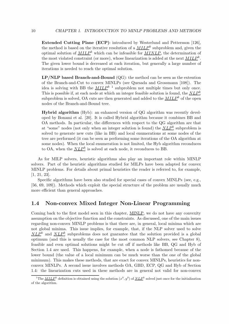
Extended Cutting Plane (ECP): introduced by Westerlund and Pettersson [126],the method is based on the iterative resolution of a MILP k subproblem and, given theoptimal solution of MILP k which can be infeasible for MINLP , the determination ofthe most violated constraint (or more), whose linearization is added at the next MILP k.The given lower bound is decreased at each iteration, but generally a large number ofiterations is needed to reach the optimal solution.

LP/NLP based Branch-and-Bound (QG): the method can be seen as the extentionof the Branch-and-Cut to convex MINLPs (see Quesada and Grossmann [108]). Theidea is solving with BB the MILP k 1 subproblem not multiple times but only once.This is possible if, at each node at which an integer feasible solution is found, the NLP k

x

subproblem is solved, OA cuts are then generated and added to the MILP k of the opennodes of the Branch-and-Bound tree.

Hybrid algorithm (Hyb): an enhanced version of QG algorithm was recently devel-oped by Bonami et al. [20]. It is called Hybrid algorithm because it combines BB andOA methods. In particular, the differences with respect to the QG algorithm are thatat “some” nodes (not only when an integer solution is found) the NLP k

x subproblem issolved to generate new cuts (like in BB) and local enumerations at some nodes of thetree are performed (it can be seen as performing some iterations of the OA algorithm atsome nodes). When the local enumeration is not limited, the Hyb algorithm reconducesto OA, when the NLP k

x is solved at each node, it reconduces to BB.

As for MILP solvers, heuristic algorithms also play an important role within MINLPsolvers. Part of the heuristic algorithms studied for MILPs have been adapted for convexMINLP problems. For details about primal heuristics the reader is referred to, for example,[1, 21, 23].

Specific algorithms have been also studied for special cases of convex MINLPs (see, e.g.,[56, 69, 109]). Methods which exploit the special structure of the problem are usually muchmore efficient than general approaches.

1.4 Non-convex Mixed Integer Non-Linear Programming

Coming back to the first model seen in this chapter, MINLP, we do not have any convexityassumption on the objective function and the constraints. As discussed, one of the main issuesregarding non-convex MINLP problems is that there are, in general, local minima which arenot global minima. This issue implies, for example, that, if the NLP solver used to solveNLP k and NLP k

x subproblems does not guarantee that the solution provided is a globaloptimum (and this is usually the case for the most common NLP solvers, see Chapter 8),feasible and even optimal solutions might be cut off if methods like BB, QG and Hyb ofSection 1.4 are used. This happens, for example, when a node is fathomed because of thelower bound (the value of a local minimum can be much worse than the one of the globalminimum). This makes these methods, that are exact for convex MINLPs, heuristics for non-convex MINLPs. A second issue involves methods OA, GBD, ECP, QG and Hyb of Section1.4: the linearization cuts used in these methods are in general not valid for non-convex

1The MILP k definition is obtained using the solution (x0, y0) of NLP k solved just once for the initializationof the algorithm.

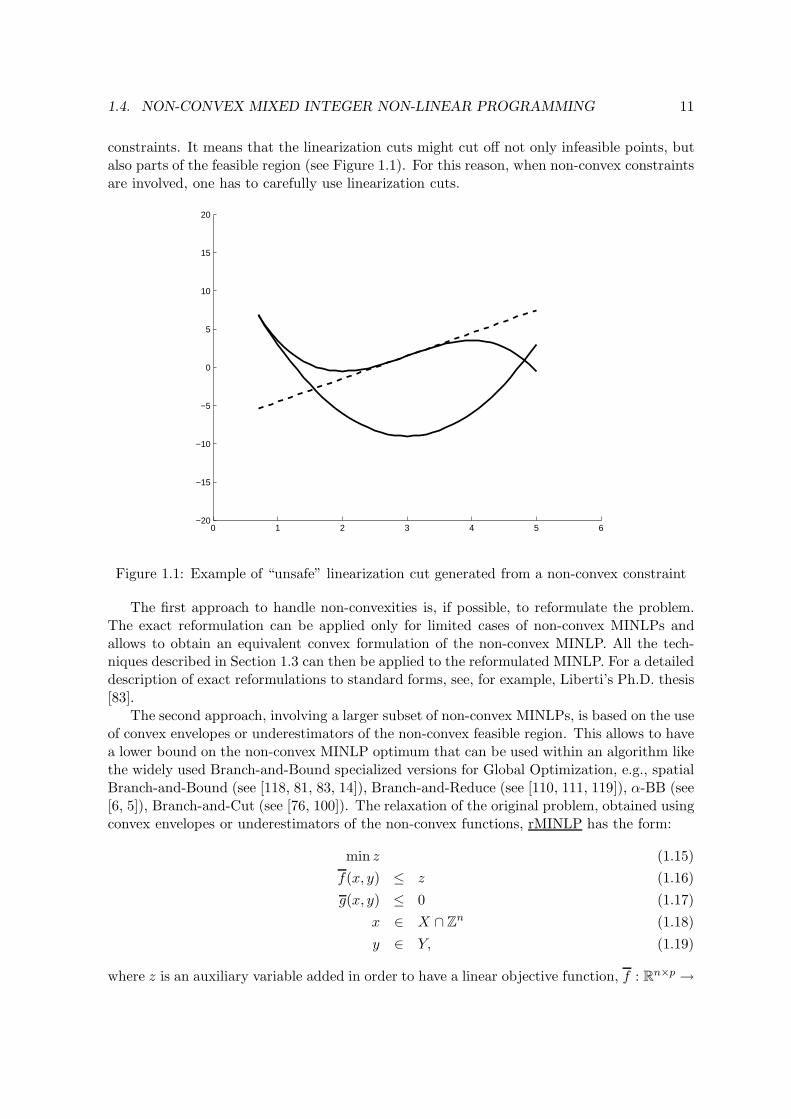
1.4. NON-CONVEX MIXED INTEGER NON-LINEAR PROGRAMMING 11

constraints. It means that the linearization cuts might cut off not only infeasible points, butalso parts of the feasible region (see Figure 1.1). For this reason, when non-convex constraintsare involved, one has to carefully use linearization cuts.

0 1 2 3 4 5 6−20

−15

−10

−5

0

5

10

15

20

Figure 1.1: Example of “unsafe” linearization cut generated from a non-convex constraint

The first approach to handle non-convexities is, if possible, to reformulate the problem.The exact reformulation can be applied only for limited cases of non-convex MINLPs andallows to obtain an equivalent convex formulation of the non-convex MINLP. All the tech-niques described in Section 1.3 can then be applied to the reformulated MINLP. For a detaileddescription of exact reformulations to standard forms, see, for example, Liberti’s Ph.D. thesis[83].

The second approach, involving a larger subset of non-convex MINLPs, is based on the useof convex envelopes or underestimators of the non-convex feasible region. This allows to havea lower bound on the non-convex MINLP optimum that can be used within an algorithm likethe widely used Branch-and-Bound specialized versions for Global Optimization, e.g., spatialBranch-and-Bound (see [118, 81, 83, 14]), Branch-and-Reduce (see [110, 111, 119]), α-BB (see[6, 5]), Branch-and-Cut (see [76, 100]). The relaxation of the original problem, obtained usingconvex envelopes or underestimators of the non-convex functions, rMINLP has the form:

min z (1.15)

f(x, y) ≤ z (1.16)

g(x, y) ≤ 0 (1.17)

x ∈ X ∩ Zn (1.18)

y ∈ Y, (1.19)

where z is an auxiliary variable added in order to have a linear objective function, f : Rn×p →


R and g : Rn×p → R

m are convex (in some cases, linear) functions and f(x, y) ≤ f(x, y) andg(x, y) ≤ g(x, y) within the (x, y) domain.

Explanations on different ways to define functions f(x, y) and g(x, y) for non-convex func-tions f and g with specific structure can be found, for example, in [83, 92, 98]. Note anywaythat, in general, these techniques apply only for factorable functions, i.e. function which canbe expressed as summations and products of univariate functions, which can be reduced andreformulated as predetermined operators for which convex underestimators are known, suchas, for example, bilinear, trilinear, fractional terms (see [84, 92, 118]).

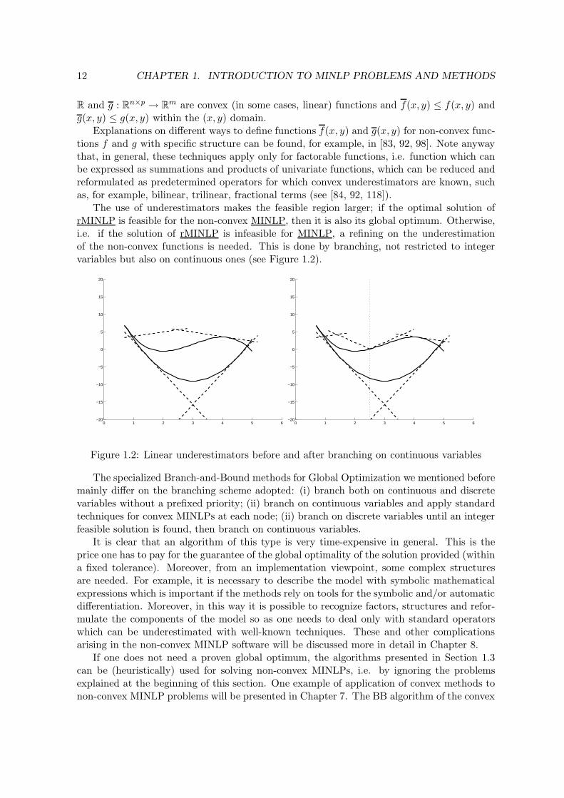
The use of underestimators makes the feasible region larger; if the optimal solution ofrMINLP is feasible for the non-convex MINLP, then it is also its global optimum. Otherwise,i.e. if the solution of rMINLP is infeasible for MINLP, a refining on the underestimationof the non-convex functions is needed. This is done by branching, not restricted to integervariables but also on continuous ones (see Figure 1.2).

0 1 2 3 4 5 6−20

−15

−10

−5

0

5

10

15

20

0 1 2 3 4 5 6−20

−15

−10

−5

0

5

10

15

20

Figure 1.2: Linear underestimators before and after branching on continuous variables

The specialized Branch-and-Bound methods for Global Optimization we mentioned beforemainly differ on the branching scheme adopted: (i) branch both on continuous and discretevariables without a prefixed priority; (ii) branch on continuous variables and apply standardtechniques for convex MINLPs at each node; (ii) branch on discrete variables until an integerfeasible solution is found, then branch on continuous variables.

It is clear that an algorithm of this type is very time-expensive in general. This is theprice one has to pay for the guarantee of the global optimality of the solution provided (withina fixed tolerance). Moreover, from an implementation viewpoint, some complex structuresare needed. For example, it is necessary to describe the model with symbolic mathematicalexpressions which is important if the methods rely on tools for the symbolic and/or automaticdifferentiation. Moreover, in this way it is possible to recognize factors, structures and refor-mulate the components of the model so as one needs to deal only with standard operatorswhich can be underestimated with well-known techniques. These and other complicationsarising in the non-convex MINLP software will be discussed more in detail in Chapter 8.

If one does not need a proven global optimum, the algorithms presented in Section 1.3can be (heuristically) used for solving non-convex MINLPs, i.e. by ignoring the problemsexplained at the beginning of this section. One example of application of convex methods tonon-convex MINLP problems will be presented in Chapter 7. The BB algorithm of the convex

1.5. GENERAL CONSIDERATIONS ON MINLPS 13

MINLP solver Bonmin [26], modified to limit the effects of non-convexities, was used. Someof these modifications were implemented in Bonmin while studying the application describedin Chapter 7 and are now part of the current release.

Also in this case, heuristics studied originally for MILPs have been adapted for non-convexMINLPs. An example is given by a recent work of Liberti et al. [86]. In Chapter 2 we willpresent a new heuristic algorithm extending to non-convex MINLPs the Feasibility Pump(FP) heuristic ideas for MILPs and convex MINLPs. Using some of the basic ideas of theoriginal FP for solving non-convex MINLPs is not possible for the same reasons we explainedbefore. Also in this case algorithms studied for convex MINLPs encounter problems whenapplied to non-convex MINLPs. In Chapter 2 we will explain in detail how we can limit thesedifficulties.

Specific algorithms have been also studied for special cases of non-convex MINLPs (see,e.g., [73, 107, 113]). As for convex MINLPs, methods which exploit the special structure ofthe problem are usually much more efficient than general approaches. Examples are given inChapters 3.

1.5 General considerations on MINLPs

Until recent years, the standard approach for handling MINLP problems has basically beensolving an MILP approximation of it. In particular, linearization of the non-linear constraintscan be applied. Note, however, that this approach differs from, e.g., OA, GBD and ECPpresented in Section 1.3 because the linearization is decided before the optimization starts,the definition of the MILP problem is never modified and no NLP (sub)problem resolution isperformed. This allows using all the techniques described in Section 1.1, which are in generalmuch more efficient than the methods studied for MINLPs. The optimal solution of the MILPmight be neither optimal nor feasible for the original problem, if no assumptions are doneof the MINLPs. If, for example, f(x, y) is approximated with a linear objective function,say f(x, y), and g(x, y) with linear functions, say g(x, y), such that f(x, y) ≥ f(x, y) andg(x, y) ≥ g(x, y), the MILP approximation provide a lower bound on the original problem.Note that, also in this case, the optimum of the MILP problem is not guaranteed to befeasible for the original MINLP, but, in case it is feasible for the MINLP problem, we havethe guarantee that it is also the global optimum.

In Chapter 4, a method for approximating non-linear functions of two variables is pre-sented: comparisons to the more classical methods like piecewise linear approximation andtriangulation are reported. In Chapter 6 we show an example of application in which applyingthese techniques is successful. We will show when it is convenient applying MINLP techniquesin Chapter 7.

Finally, note that the integrality constraint present in Mixed Integer Programming prob-lems can be seen as a source of non-convexity for the problem: it is possible to map thefeasibility problem of an MILP problem into an NLP problem. Due to this consideration, westudied NLP-based heuristics for MILP problems: these ideas are presented in Chapter 5.


Part II

Modeling and SolvingNon-Convexities

15

Chapter 2

A Feasibility Pump Heuristic forNon-Convex MINLPs

1

2.1 Introduction

Heuristic algorithms have always played a fundamental role in optimization, both as inde-pendent tools and as part of general-purpose solvers. Starting from Mixed Integer LinearProgramming (MILP), different kinds of heuristics have been proposed: their aim is findinga good feasible solution rapidly or improving the best solution found so far. Within a MILPsolver context, both types of heuristics are used. Examples of heuristic algorithms are round-ing heuristics, metaheuristics (see, e.g., [63]), Feasibility Pump [50, 16, 3], Local Branching[51] and Relaxation Induced Neighborhoods Search [43]. Even if the heuristic algorithmsmight find the optimal solution, no guarantee on the optimality is given.

In the most recent years Mixed Integer Non-Linear Programming (MINLP) has become atopic capable of attracting the interest of the research community. This is due from the oneside to the continuous improvements of Non-Linear Programming (NLP) solvers and on theother hand to the wide range of real-world applications involving these problems. A specialfocus has been devoted to convex MINLPs, a class of MINLP problems whose nice propertiescan be exploited. In particular, under the convexity assumption, any local optimum is also aglobal optimum of the continuous relaxation and the use of standard linearization cuts likeOuter Approximation (OA) cuts [45] is possible, i.e. the generated cuts are valid. Heuristicshave been proposed recently also for this class of problems. Basically the ideas originallytailored on MILP problems have been extended to convex MINLPs, for example, FeasibilityPump [21, 1, 23] and diving heuristics [23].

The focus of this chapter is proposing a heuristic algorithm for non-convex MINLPs. Theseproblems are in general very difficult to solve to optimality and, usually, like sometimes alsohappens for MILP problems, finding any feasible solution is also a very difficult task inpractice (besides being NP-hard in theory). For this reason, heuristic algorithms assume afundamental part of the solving phase. Heuristic algorithms proposed so far for non-convexMINLPs are, for example, Variable Neighborhood Search [86] and Local Branching [93], but

1This is a working paper with Antonio Frangioni (DI, University of Pisa), Leo Liberti (LIX, Ecole Poly-technique) and Andrea Lodi (DEIS, University of Bologna).

17

18 CHAPTER 2. A FEASIBILITY PUMP HEURISTIC FOR NON-CONVEX MINLPS

this field is still highly unexplored. This is mainly due to the difficulties arising from the lackof structures and properties to be exploited for such a general class of problems.

We already mentioned the innovative approach to the feasibility problem for MILPs, calledFeasibility Pump, which was introduced by Fischetti et al. [50] for problems with integer vari-ables restricted to be binary and lately extended to general integer by Bertacco et al. [16].The idea is to iteratively solve subproblems of the original difficult problem with the aim of“pumping” the feasibility in the solution. More precisely, Feasibility Pump solves the conti-nous relaxation of the problem trying to minimize the distance to an integer solution, thenrounding the fractional solution obtained. Few years later a similar technique applied to con-vex MINLPs was proposed by Bonami et al. [21]. In this case, at each iteration, an NLP andan MILP subproblems are solved. The authors also prove the convergence of the algorithmand extend the same result to MINLP problems with non-convex constraints, defining, how-ever, a convex feasible region. More recently Bonami and Goncalves [23] proposed a less timeconsuming version in which the MILP resolution is substituted by a rounding phase similarto that originally proposed by Fischetti et al. [50] for MILPs.

In this chapter, we propose a Feasibility Pump algorithm for general non-convex MINLPsusing ingredients of the previous versions of the algorithm and adapting them in order toremove assumptions about any special structure of the problem. The remainder of the chapteris organized as follows. In Section 2.2 we present the structure of the algorithm, then wedescribe in detail each part of it. Details on algorithm (implementation) issues are given inSection 2.3. In Section 2.4 we present computational results on MINLPLib instances. Finally,in Section 2.5, we draw conclusions and discuss future work directions.

2.2 The algorithm

The problem which we address is the non-convex MINLP problem of the form:

(P ) min f(x, y) (2.1)

g(x, y) ≤ 0 (2.2)

x ∈ X ∩ Zn (2.3)

y ∈ Y, (2.4)

where X and Y are two polyhedra of appropriate dimension (including bounds on the vari-ables), f : R

n+p → R is convex, but g : Rn+p → R

m is non-convex. We will denote byP = { (x, y) | g(x, y) ≤ 0 } ⊆ R

n+p the (non-convex) feasible region of the continuousrelaxation of the problem, by X the set {1, . . . , n} and by Y the set {1, . . . , p}. We willalso denote by NC ⊆ {1, . . . ,m} the subset of (indices of) non-convex constraints, so thatC = {1, . . . ,m} \ NC is the set of (indices of) “ordinary” convex constraints. Note that theconvexity assumption on the objective function f can be taken without loss of generality; onecan always introduce a further variable v, to be put alone in the objective function, and addthe (m + 1)th constraint f(x, y) − v ≤ 0 to deal with the case where f is non-convex.

The problem (P ) presents two sources of non-convexities:

1. integrality requirements on x variables;

2. constraints gj(x, y) ≤ 0 with j ∈ NC, defining a non-convex feasible region, even if wedo not consider the integrality requirements on x variables.

2.2. THE ALGORITHM 19

The basic idea of Feasibility Pump is decomposing the original problem in two easiersubproblems, one obtained relaxing integrality constraints, the other relaxing “complicated”constraints. At each iteration a pair of solutions (x, y) and (x, y) is computed, the solutionof the first subproblem and the second one, respectively. The aim of the algorithm is makingthe trajectories of the two solutions converge to a unique point, satisfying all the constraintsand the integrality requirements (see Algorithm 1).

Algorithm 1 The general scheme of Feasibility Pump

1: i=0;2: while (((xi, yi) 6= (xi, yi)) ∧ time limit) do3: Solve the problem (P1) obtained relaxing integrality requirements (using all other con-

straints) and minimizing a “distance” with respect to (xi, yi);4: Solve the problem (P2) obtained relaxing “complicated” constraints (using the inte-

grality requirements) minimizing a “distance” with respect to (xi, yi);5: i++;6: end while

When the original problem (P ) is a MILP, (P1) is simply the LP relaxation of the prob-lem and solving (P2) corresponds to a rounding of the fractional solution of (P1) (all theconstraints are relaxed, see Fischetti et al. [50]). When the original problem (P ) is a MINLP,(P1) is the NLP relaxation of the problem and (P2) a MILP relaxation of (P ). If MINLP isconvex, i.e. NC = ∅, we know that (P1) is convex too and it can ideally be solved to globaloptimality and that (P2) can be “safely” defined as the Outer Approximation of (P ) (see,e.g., Bonami et al. [21]) or a rounding phase (see Bonami and Goncalves [23]).

When NC 6= ∅, things get more complicated:

the solution provided by the NLP solver for problem (P1) might be only a local minimuminstead of a global one. Suppose that the global solution of problem (P1) value is 0(i.e. it is an integer feasible solution), but the solver computes a local solution of valuegreater than 0. The OA cut generated from the local solution might mistakenly cut theinteger feasible solution.

Outer Approximation cuts can cut off feasible solutions of (P ), so these cuts can beadded to problem (P2) only if generated from constraints with “special characteristics”(which will be presented in detail in Section 2.2.2). This difficulty has implications alsoon the possibility of cycling of the algorithm.

We will discuss these two issues and how we limit their impact in the next two sections.

2.2.1 Subproblem (P1)

At iteration i subproblem (P1), denoted as (P1)i, has the form:

min ||x − xi|| (2.5)

g(x, y) ≤ 0 (2.6)

where (xi, yi) is the solution of subproblem (P2)i (see Section 2.2.2). The motivation forsolving problem (P1)i is twofold: (i) testing the compatibility of values xi with a feasiblesolution of problem (P ) (such a solution exists if the solution value of (P1)i is 0); (ii) if no


feasible solution with x variables assuming values xi, a feasible solution for P is computedminimizing the distance ||x − xi||. As anticipated in the previous section, when g(x, y) arenon-convex functions (P1)i, has, in general, local optima, i.e. solutions which are optimalconsidering a restricted part of feasible region (neighborhood). Available NLP solvers usuallydo not guarantee to provide the global optimum, i.e. an optimal solution with respect to thewhole feasible region. Moreover, solving a non-convex NLP to global optimality is in generalvery time consuming. Then, the first choice was to give up trying to solve (P1)i to globaloptimality. The consequences of this choice are that, when a local optimum is provided assolution of (P1)i and its value is greater than 0, there might be a solution of (P ) with valuesxi, i.e. the globally optimal solution might have value 0. In this case we would, mistakenly,cut off a feasible solution of (P ). To limit this possibility we decided to divide step 3 ofAlgorithm 1 in two parts:

1. Solve (P1)i to local optimality, but multiple times, i.e. using randomly generated start-ing points;

2. If no solution was found, then solve (P1fix)i:

min f(xi, y) (2.7)

g(xi, y) ≤ 0 (2.8)

Note that objective function (2.5) is useless when variables x are fixed to xi, so we canuse the original objective function or, alternatively, a null function or a function whichhelps the NLP solver to reach feasibility.

The solution proposed does not give any guarantee that the global optimum will be foundand, consequentely, that no feasible solution of (P ) will be ignored, but, since we proposea heuristic algorithm, we consider this simplification as a good compromise. Note, however,that for some classes of non-convex MINLP the solution does the job. Consider, for example, aproblem (P ) that, once variables x are fixed, is convex: in this case solving problem (P1fix)i

would provide the global optimum. In Section 2.4 we will provide details on the computationalbehavior of the proposed solution.

2.2.2 Subproblem (P2)

At iteration i subproblem (P2), denoted as (P2)i, has the form:

min ||x − xi−1|| (2.9)

gj(xk, yk) + ∇gj(x

k, yk)T[

x − xk

y − yk

]≤ 0 k = 1, . . . , i − 1; j ∈ Mk (2.10)

x ∈ Zn (2.11)

y ∈ Rp, (2.12)

where (xi−1, yi−1) is the solution of subproblem (P1)i−1 and Mk ⊆ {1, . . . ,m} is the setof (indices of) constraints from which OA cuts are generated from point (xk, yk). We limitthe OA cuts added to (P2) because, when non-convex constraints are involved, not all thepossible OA cuts generated are “safe”, i.e. do not cut off feasible solutions of (P ) (see Figure6.1).


(x0,y0)

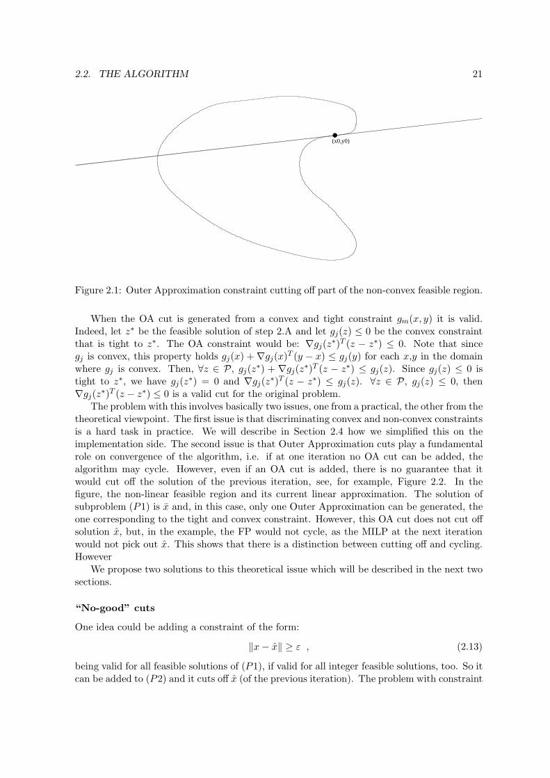
Figure 2.1: Outer Approximation constraint cutting off part of the non-convex feasible region.

When the OA cut is generated from a convex and tight constraint gm(x, y) it is valid.Indeed, let z∗ be the feasible solution of step 2.A and let gj(z) ≤ 0 be the convex constraintthat is tight to z∗. The OA constraint would be: ∇gj(z

∗)T (z − z∗) ≤ 0. Note that sincegj is convex, this property holds gj(x) + ∇gj(x)T (y − x) ≤ gj(y) for each x,y in the domainwhere gj is convex. Then, ∀z ∈ P, gj(z

∗) + ∇gj(z∗)T (z − z∗) ≤ gj(z). Since gj(z) ≤ 0 is

tight to z∗, we have gj(z∗) = 0 and ∇gj(z

∗)T (z − z∗) ≤ gj(z). ∀z ∈ P, gj(z) ≤ 0, then∇gj(z

∗)T (z − z∗) ≤ 0 is a valid cut for the original problem.The problem with this involves basically two issues, one from a practical, the other from the

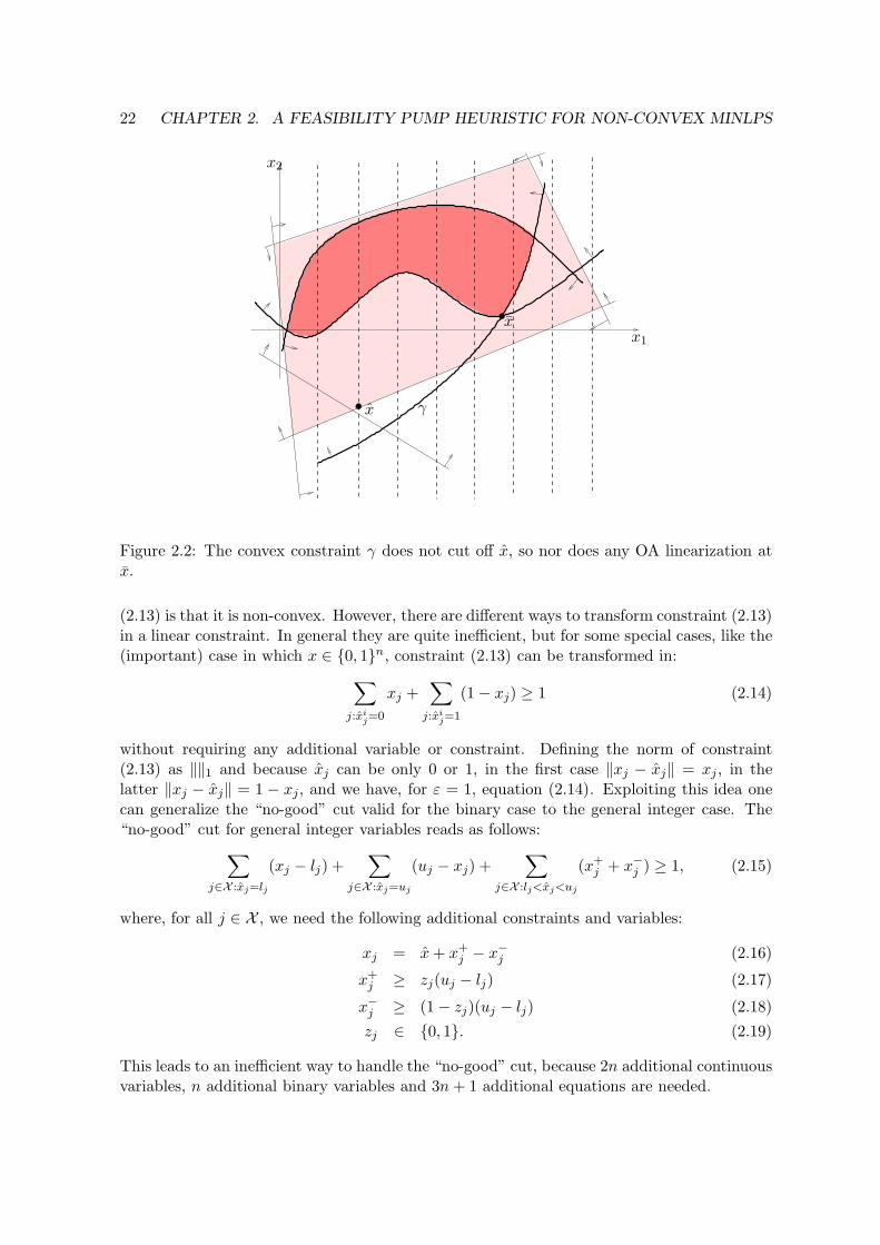
theoretical viewpoint. The first issue is that discriminating convex and non-convex constraintsis a hard task in practice. We will describe in Section 2.4 how we simplified this on theimplementation side. The second issue is that Outer Approximation cuts play a fundamentalrole on convergence of the algorithm, i.e. if at one iteration no OA cut can be added, thealgorithm may cycle. However, even if an OA cut is added, there is no guarantee that itwould cut off the solution of the previous iteration, see, for example, Figure 2.2. In thefigure, the non-linear feasible region and its current linear approximation. The solution ofsubproblem (P1) is x and, in this case, only one Outer Approximation can be generated, theone corresponding to the tight and convex constraint. However, this OA cut does not cut offsolution x, but, in the example, the FP would not cycle, as the MILP at the next iterationwould not pick out x. This shows that there is a distinction between cutting off and cycling.However

We propose two solutions to this theoretical issue which will be described in the next twosections.

“No-good” cuts

One idea could be adding a constraint of the form:

‖x − x‖ ≥ ε , (2.13)

being valid for all feasible solutions of (P1), if valid for all integer feasible solutions, too. So itcan be added to (P2) and it cuts off x (of the previous iteration). The problem with constraint


x

xx1

x2

γ

Figure 2.2: The convex constraint γ does not cut off x, so nor does any OA linearization atx.

(2.13) is that it is non-convex. However, there are different ways to transform constraint (2.13)in a linear constraint. In general they are quite inefficient, but for some special cases, like the(important) case in which x ∈ {0, 1}n, constraint (2.13) can be transformed in:

∑

j:xij=0

xj +∑

j:xij=1

(1 − xj) ≥ 1 (2.14)

without requiring any additional variable or constraint. Defining the norm of constraint(2.13) as ‖‖1 and because xj can be only 0 or 1, in the first case ‖xj − xj‖ = xj , in thelatter ‖xj − xj‖ = 1 − xj, and we have, for ε = 1, equation (2.14). Exploiting this idea onecan generalize the “no-good” cut valid for the binary case to the general integer case. The“no-good” cut for general integer variables reads as follows:

∑

j∈X :xj=lj

(xj − lj) +∑

j∈X :xj=uj

(uj − xj) +∑

j∈X :lj<xj<uj

(x+j + x−

j ) ≥ 1, (2.15)

where, for all j ∈ X , we need the following additional constraints and variables:

xj = x + x+j − x−

j (2.16)

x+j ≥ zj(uj − lj) (2.17)

x−j ≥ (1 − zj)(uj − lj) (2.18)

zj ∈ {0, 1}. (2.19)

This leads to an inefficient way to handle the “no-good” cut, because 2n additional continuousvariables, n additional binary variables and 3n + 1 additional equations are needed.


This MILP formulation of the “no-good” cut for general integer can be seen as the interval-gradient cut of constraint (2.13) using ‖‖1 and ε = 1.

In the following we present some considerations about the relationship between the interval-gradient cut (see [98]) and the “no-good” cut proposed (2.15)-(2.19). Suppose we have anon-convex constraint g(x) ≤ 0 with x ∈ [x, x] and that [d, d] is the interval-gradient of gover [x, x], i.e. ∇g(x) ∈ [d, d] for x ∈ [x, x]. The interval-gradient cut generated from thisconstraint with respect to a point x is:

g(x) = g(x) + mind∈[d,d]

dT (x − x) ≤ 0. (2.20)

(Here we are exploiting the following property: g(x) ≤ g(x) ≤ 0, then we know the cut isvalid.) Equation (2.20) can be reformulated with the following MILP model:

g(x) +∑

j∈X

(dx+ − dx−) ≤ 0 (2.21)

x − x = x+ − x− (2.22)

x+j ≤ zj(xj − xj) j ∈ X (2.23)

x−j ≤ (1 − zj)(xj − xj) j ∈ X (2.24)

x+ ≥ 0, x− ≥ 0 (2.25)

z ∈ {0, 1}n (2.26)

with the cost of 2n additional continuous variables, n additional binary variables and 3n + 1additional constraints. Now, consider equation (2.13). It is non-convex and we try to generatean interval-gradient cut with respect to point x. We first transform equation (2.13) in thisway (using ‖‖1 and ε = 1):

g(x) ≤ g(x) = −∑

j∈X

|xj − xj | ≤ −1 . (2.27)

First consideration: g(x) = 0. Now let analyze a particular index j ∈ X . Three cases arepossible:

1. xj = xj: this implies that −|xj − xj| = xj −xj and d = d = −1. The term (dx+j − dx−

j )

become −x+j + x−

j = −xj + xj = xj − xj.

2. xj = xj: this implies that −|xj − xj| = xj − xj and d = d = 1. The term (dx+j − dx−

j )

become x+j − x−

j = xj − +xj = xj − xj.

3. xj ≤ xj ≤ xj: this implies that d = −1 and d = 1. The term (dx+j − dx−

j ) become

−(x+j + x−

j ).

We can then simplify equation (2.21) in this way:

∑

j∈X :xj=xj

(xj − xj) +∑

j∈X :xj=xj

(xj − x) +∑

j∈X :xj<xj<xj

(−x+j − x−

j ) ≤ −1 (2.28)


changing the sign and completing the MILP model:∑

j∈X :xj=xj

(xj − xj) +∑

j∈X :xj=xj

(x − xj) +∑

j∈X :xj<xj<xj

(x+j + x−

j ) ≥ 1 (2.29)

x+j ≤ zj(xj − xj) j ∈ X (2.30)

x−j ≤ (1 − zj)(xj − xj) j ∈ X (2.31)

x+ ≥ 0, x− ≥ 0 (2.32)

z ∈ {0, 1}n (2.33)

which is exactly the “no-good” cut for general integer.In the following we present the details of how to linearize the “no-good” cut (2.13) in thegeneral integer case. In particular we considered two cases:

1. Using ‖ · ‖∞ for problem (P1);

2. Using ‖ · ‖1 for problem (P1).

We explicitly define the NLP problems for the two cases:

(NLP ) (x, y) = argmin{ ‖x − x‖∞ : g(x, y) ≤ 0 } =

argmin{ ε : −ε ≤ xi − xi ≤ ε ∀i, ε ≥ 0, g(x, y) ≤ 0 }

(NLP ) (x, y) = argmin{ ‖x − x‖1 : g(x, y) ≤ 0 } =

argmin{ ε =∑

i

vi : −vi ≤ xi − xi ≤ vi ∀i, v ≥ 0, g(x, y) ≤ 0 }.

In both the cases, if the objective function value of the optimal solution of NLP is equal to 0,we have an integer and feasible solution that is x. If this is not the case, we have to solve theMILP problem, but we want to add something that avoid the possible cycling. If there aresome convex constraints that are tight for (x, y), we can generate the OA constraints that isadded to the MILP problem of the previous iteration and we will get a new (xk, yk). If thereis no convex constraint that is tight, we will solve one of these two problems (resp, for the‖ · ‖∞ and ‖ · ‖1 cases):

(MILP k) (xk, yk) = argmin{ ‖x − x‖ : gj(xk, yk) + ∇gj(x

k, yk)T[

x − xk

y − yk

]≤ 0

k = 1, . . . , i − 1; j ∈ Mk, ⌈ε⌉ ≤ xi − xk−1i + M(1 − zi) ∀i,

⌈ε⌉ ≤ xk−1i − xi + M(1 − z′i) ∀i,

∑

i

zi +∑

i

z′i ≥ 1, z ∈ {0, 1}p, z′ ∈ {0, 1}p }

(Intuitively, if zi (or z′i) is equal to 1, the correspondent constraint is active and we imposethat the component i is changed wrt xk−1)

(MILP k) (xk, yk) = argmin{ ‖x − x‖ : gj(xk, yk) + ∇gj(x

k, yk)T[

x − xk

y − yk

]≤ 0

k = 1, . . . , i − 1; j ∈ Mk, vi ≤ xi − xk−1i + Mzi ∀i,

vi ≤ xk−1i − xi + M(1 − zi) ∀i,

∑

i

vi ≥ ⌈ε⌉, z ∈ {0, 1}p }

2.3. SOFTWARE STRUCTURE 25

(Intuitively, if vi is greater than 0, one of the 2 correspondent constraints is active and weimpose that the component i is changed wrt xk−1. The minimum total change is ⌈ε⌉).where ε is the objective function value of the optimal solution of NLP, xk−1 is the optimalsolution of MILP at the previous iteration, M is the big M coefficient that has to be definedin a clever way.

Tabu list

An alternative way, which do not involve modifications of the model such as introducingadditional variables and complicated constraints, is using a tabu list of the last solutionscomputed by (P2). From a practical viewpoint this is possible using a feature availablewithin the MILP solver Ilog Cplex [71] called “callback”. The one we are interested in is the“incumbent callback”, a tool which allows the user to define a function which is called duringthe execution of the Branch-and-Bound whenever Cplex finds a new integer feasible solution.Within the callback function the integer feasible solution computed by the solver is available.The integer part of the solution is compared with the one of the solutions in the tabu listand, only if the solution has a tollerable diversity with respect to the forbidden solutions, itis accepted. Otherwise it is discarted and the Branch-and-Bound execution continues. In thisway, even if the same solution can be obtained in two consequent iteration, the algorithmdiscarts it, then it does not cycle. It is a simple idea which works both with binary and withgeneral integer variables. The diversity of two solutions, say, x1 and x2, is computed in thefollowing way: ∑

j∈X

|x1j − x2

j |,

and two solutions are different if the above sum is not 0. Note that the continuous part ofthe solution does not influence the diversity measure.

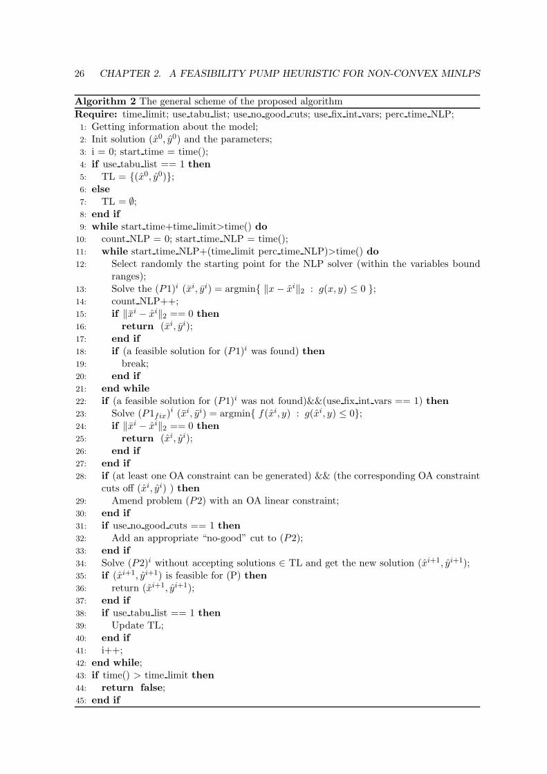
2.2.3 The resulting algorithm

The general scheme of the algorithm proposed is described by Algorithm 2. The resolution ofproblem (P1) is represented by steps 10-27 and the resolution of problem (P2) is representedby steps 28-40. At step 23, a restriction of problem (P) is solved. This restriction is “generally”a non-convex NLP we solve to local optimality, if we have no assumption on the structure ofthe problem. The objective function problem of step 34 is ‖x − xi‖1. Finally note that, ifuse tabu list is 0, TL is ∅ and no integer solution will be rejected (the “no-good” cuts do thejob).

In the next section we present details on the implementation of the algorithm.

2.3 Software structure

The algorithm was implemented within the AMPL environment [55]. We choose to use thisframework to be flexible with respect to the solver we want to use in the different phases ofthe proposed algorithm. In practice, the user can select the preferred solver to solve NLPs orMILPs, exploiting advantages of the chosen solver.

The input is composed of two files: (i) the mod file where the model of the instanceis implemented, called “fpminlp.mod”; (ii) the file “parameter.txt”, in which one can de-


Algorithm 2 The general scheme of the proposed algorithm

Require: time limit; use tabu list; use no good cuts; use fix int vars; perc time NLP;1: Getting information about the model;2: Init solution (x0, y0) and the parameters;3: i = 0; start time = time();4: if use tabu list == 1 then5: TL = {(x0, y0)};6: else7: TL = ∅;8: end if9: while start time+time limit>time() do

10: count NLP = 0; start time NLP = time();11: while start time NLP+(time limit perc time NLP)>time() do12: Select randomly the starting point for the NLP solver (within the variables bound

ranges);13: Solve the (P1)i (xi, yi) = argmin{ ‖x − xi‖2 : g(x, y) ≤ 0 };14: count NLP++;15: if ‖xi − xi‖2 == 0 then16: return (xi, yi);17: end if18: if (a feasible solution for (P1)i was found) then19: break;20: end if21: end while22: if (a feasible solution for (P1)i was not found)&&(use fix int vars == 1) then23: Solve (P1fix)i (xi, yi) = argmin{ f(xi, y) : g(xi, y) ≤ 0};24: if ‖xi − xi‖2 == 0 then25: return (xi, yi);26: end if27: end if28: if (at least one OA constraint can be generated) && (the corresponding OA constraint

cuts off (xi, yi) ) then29: Amend problem (P2) with an OA linear constraint;30: end if31: if use no good cuts == 1 then32: Add an appropriate “no-good” cut to (P2);33: end if34: Solve (P2)i without accepting solutions ∈ TL and get the new solution (xi+1, yi+1);35: if (xi+1, yi+1) is feasible for (P) then36: return (xi+1, yi+1);37: end if38: if use tabu list == 1 then39: Update TL;40: end if41: i++;42: end while;43: if time() > time limit then44: return false;45: end if

2.4. COMPUTATIONAL RESULTS 27

fine parameters of step 2, the NLP solver (NLP solver), the precision ( FP epsilon andFP perc infeas allowed), the level of verbosity (VERBOSE ).

To solve problem (P1) and the restriction of step 23, we use the NLP solver as a black-box.We use solvers directly providing an AMPL interface, which is anyway usually the case forthe most common and efficient NLP solvers.

To solve problem (P2), if use tabu list is 0, we use an MILP solver as a black-box. Theinteraction with the MILP solver is done in the same way of NLP solver for (P1). Whenuse tabu list is 1, we use an executable called “tabucplex” to solve problem (P2). As antic-ipated in Section 2.2.2, we implemented this modification to a standard Branch-and-Boundmethod within the Ilog Cplex environment, exploiting the so-called callbacks. This file readsand stores data of an input file produced within the AMPL framework which contains thetabu list, i.e. the list of the “forbidden” solutions. Then the Branch-and-Bound starts: itsexecution is standard until an integer feasible solution is found. Every time an integer feasiblesolution is found, the specialized incumbent callback is called. The aim of this function isto check if the solution found is within those solutions in the tabu list, i.e. it was providedas problem (P2) solution in one of the previous iterations. If this is the case, the solution isrejected, otherwise the solution is accepted. In any case, the execution of the Branch-and-Bound continues until the optimal solution, excluding the forbidden ones, is found or a timelimit is reached.

Another tool we extensively used is a new solver/reformulator called Rose (Reformula-tion/Optimization Software Engine, see [85]), of which we exploited the following nice features:

1. Analyzing the model, i.e. getting information about non-linearity and convexity of theconstraints and integrality requirements of the variables: necessary at step 1. Theseparameters are provided by Rose as AMPL suffixes.

2. Analyzing feasibility of the solution: necessary after steps 13, 23 and for step 35 toverify feasibility of the provided solutions. Also in this case parameters are provided byRose as AMPL suffixes.

3. Generating the Outer Approximation cuts: necessary at step 29. Cuts are written in afile which is then included within the AMPL framework.

Actually some of these features were implemented within the context of this work. Notethat information about the convexity of the constraints are hard to compute: in particular,Rose gives information about the “evidently convex”/“evidently concave” constraints usingthe expression tree, properties of convex/concave functions and basic expressions (see [85] fordetails). In practice, a non-convex constraint is always identified, a convex constraint can betreated as non-convex constraint, but the information provided is in any case “safe” for ourpurposes, i.e. we generate OA cuts only from constraints which are “certified” to be convex.

An obvious modification of the algorithm proposed is considering the original objectivefunction to improve the provided solution quality as done, for example, in [50] and [21].

2.4 Computational results

In this section preliminary computational results are presented on an Intel Xeon 2.4 GHz with8 GB RAM running Linux. We stop the algorithm after the first MINLP feasible solutionwas found (or the time limit is reached). The parameters were set in the following way:


time limit = 2 hours;

use tabu list = 1;

use no good cuts = 0;

use fix int vars = 1;

perc time NLP = 0.05;

FP epsilon = 1e-6;

FP perc infeas allowed = 0.001;

The NLP solver used is Ipopt 3.5 trunk [123] and the problems solved are 243 instances takenfrom MINLPLib [32] (the ones used in [86] minus oil and oil2 because function log10 is notsupported by Rose). Tabucplex uses the Callable library of Ilog Cplex 11.0.

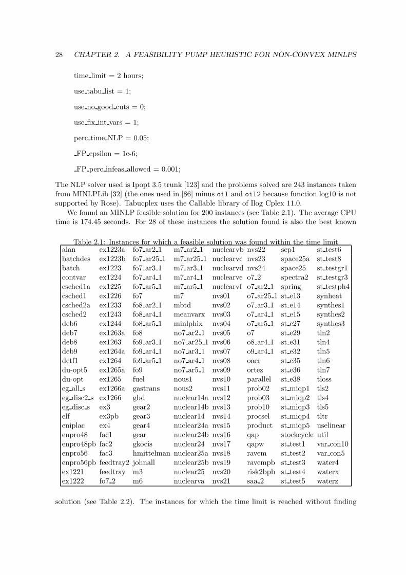
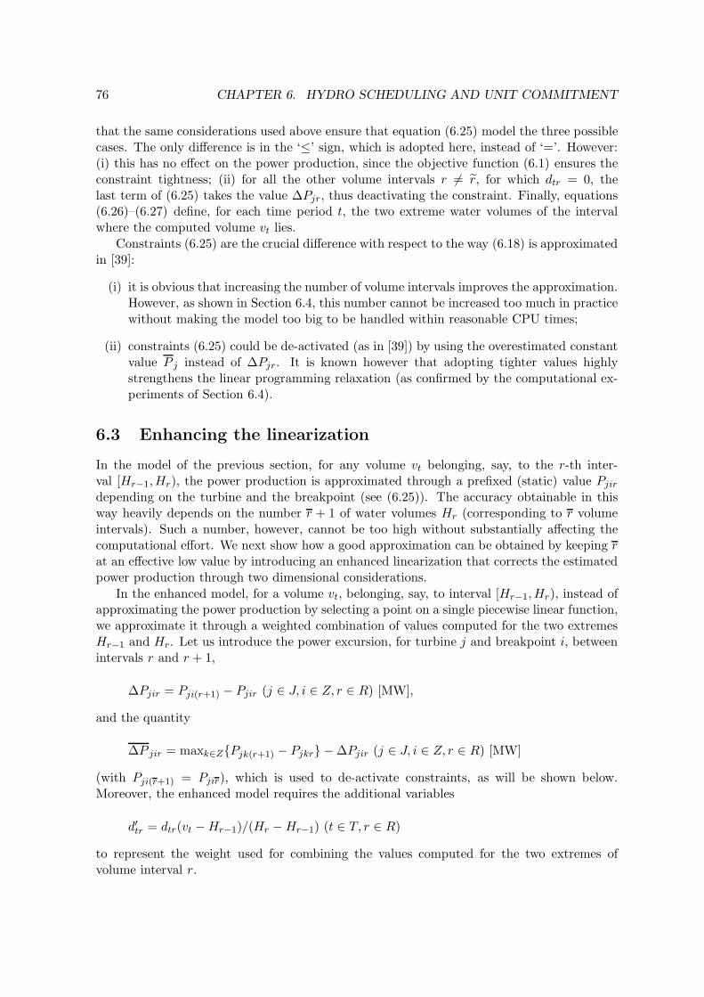
We found an MINLP feasible solution for 200 instances (see Table 2.1). The average CPUtime is 174.45 seconds. For 28 of these instances the solution found is also the best known

Table 2.1: Instances for which a feasible solution was found within the time limitalan ex1223a fo7 ar2 1 m7 ar2 1 nuclearvb nvs22 sep1 st test6batchdes ex1223b fo7 ar25 1 m7 ar25 1 nuclearvc nvs23 space25a st test8batch ex1223 fo7 ar3 1 m7 ar3 1 nuclearvd nvs24 space25 st testgr1contvar ex1224 fo7 ar4 1 m7 ar4 1 nuclearve o7 2 spectra2 st testgr3csched1a ex1225 fo7 ar5 1 m7 ar5 1 nuclearvf o7 ar2 1 spring st testph4csched1 ex1226 fo7 m7 nvs01 o7 ar25 1 st e13 synheatcsched2a ex1233 fo8 ar2 1 mbtd nvs02 o7 ar3 1 st e14 synthes1csched2 ex1243 fo8 ar4 1 meanvarx nvs03 o7 ar4 1 st e15 synthes2deb6 ex1244 fo8 ar5 1 minlphix nvs04 o7 ar5 1 st e27 synthes3deb7 ex1263a fo8 no7 ar2 1 nvs05 o7 st e29 tln2deb8 ex1263 fo9 ar3 1 no7 ar25 1 nvs06 o8 ar4 1 st e31 tln4deb9 ex1264a fo9 ar4 1 no7 ar3 1 nvs07 o9 ar4 1 st e32 tln5detf1 ex1264 fo9 ar5 1 no7 ar4 1 nvs08 oaer st e35 tln6du-opt5 ex1265a fo9 no7 ar5 1 nvs09 ortez st e36 tln7du-opt ex1265 fuel nous1 nvs10 parallel st e38 tlosseg all s ex1266a gastrans nous2 nvs11 prob02 st miqp1 tls2eg disc2 s ex1266 gbd nuclear14a nvs12 prob03 st miqp2 tls4eg disc s ex3 gear2 nuclear14b nvs13 prob10 st miqp3 tls5elf ex3pb gear3 nuclear14 nvs14 procsel st miqp4 tltreniplac ex4 gear4 nuclear24a nvs15 product st miqp5 uselinearenpro48 fac1 gear nuclear24b nvs16 qap stockcycle utilenpro48pb fac2 gkocis nuclear24 nvs17 qapw st test1 var con10enpro56 fac3 hmittelman nuclear25a nvs18 ravem st test2 var con5enpro56pb feedtray2 johnall nuclear25b nvs19 ravempb st test3 water4ex1221 feedtray m3 nuclear25 nvs20 risk2bpb st test4 waterxex1222 fo7 2 m6 nuclearva nvs21 saa 2 st test5 waterz

solution (see Table 2.2). The instances for which the time limit is reached without finding

2.5. CONCLUSIONS 29

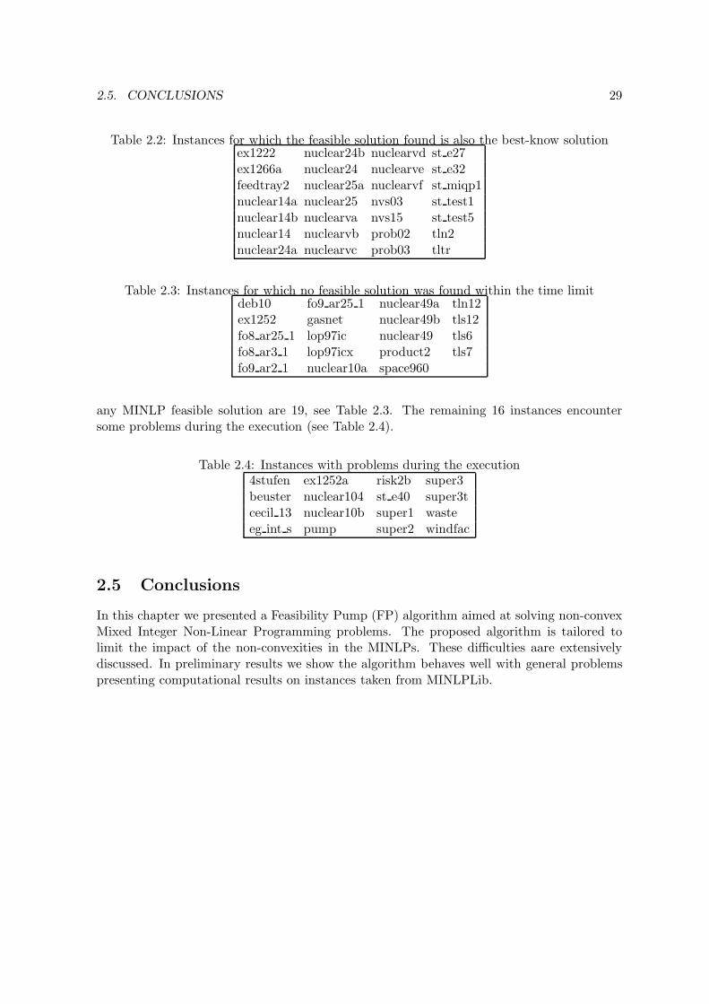
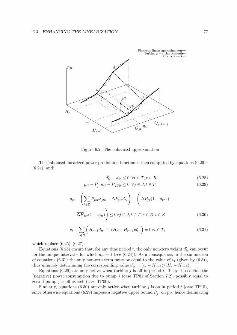
Table 2.2: Instances for which the feasible solution found is also the best-know solutionex1222 nuclear24b nuclearvd st e27ex1266a nuclear24 nuclearve st e32feedtray2 nuclear25a nuclearvf st miqp1nuclear14a nuclear25 nvs03 st test1nuclear14b nuclearva nvs15 st test5nuclear14 nuclearvb prob02 tln2nuclear24a nuclearvc prob03 tltr

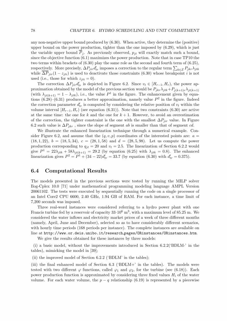
Table 2.3: Instances for which no feasible solution was found within the time limitdeb10 fo9 ar25 1 nuclear49a tln12ex1252 gasnet nuclear49b tls12fo8 ar25 1 lop97ic nuclear49 tls6fo8 ar3 1 lop97icx product2 tls7fo9 ar2 1 nuclear10a space960

any MINLP feasible solution are 19, see Table 2.3. The remaining 16 instances encountersome problems during the execution (see Table 2.4).

Table 2.4: Instances with problems during the execution4stufen ex1252a risk2b super3beuster nuclear104 st e40 super3tcecil 13 nuclear10b super1 wasteeg int s pump super2 windfac

2.5 Conclusions

In this chapter we presented a Feasibility Pump (FP) algorithm aimed at solving non-convexMixed Integer Non-Linear Programming problems. The proposed algorithm is tailored tolimit the impact of the non-convexities in the MINLPs. These difficulties aare extensivelydiscussed. In preliminary results we show the algorithm behaves well with general problemspresenting computational results on instances taken from MINLPLib.


Chapter 3

A Global Optimization Method fora Class of Non-Convex MINLPProblems

1

3.1 Introduction

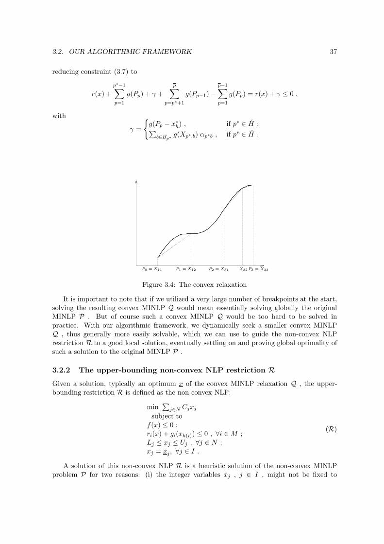
The global solution of practical instances of Mixed Integer Non-Linear Programming (MINLP)problems has been considered for some decades. Over a considerable period of time, tech-nology for the global optimization of convex MINLP (i.e. the continuous relaxation of theproblem is a convex program) had matured (see, for example, [45, 108, 20]), and rather re-cently there has been considerable success in the realm of global optimization of non-convexMINLP (see, for example, [111, 99, 84, 14]).

Global optimization algorithms, e.g., spatial Branch-and-Bound approaches like thoseimplemented in codes like BARON [111] and Couenne [14], have had substantial success intackling complicated, but generally small scale, non-convex MINLPs (i.e., mixed-integer non-linear programs having non-convex continuous relaxations). Because they are aimed at arather general class of problems, the possibility remains that larger instances from a simplerclass may be amenable to a simpler approach.

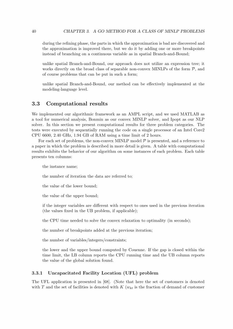
We focus on separable MINLPs, that is where the objective and constraint functions aresums of univariate functions. There are many problems that are already in such a form, orcan be brought into such a form via some simple substitutions. In fact, the first step in spatialBranch-and-Bound is to bring problems into nearly such a form. For our purposes, we shiftthat burden back to the modeler. We have developed a simple algorithm, implemented atthe level of a modeling language (in our case AMPL, see [55]), to attack such separable prob-lems. First, we identify subintervals of convexity and concavity for the univariate functionsusing external calls to MATLAB [91]. With such an identification at hand, we develop aconvex MINLP relaxation of the problem (i.e., as a mixed-integer non-linear programs havinga convex continuous relaxations). Our convex MINLP relaxation differs from those typically

1This is a working paper with Jon Lee and Andreas Wachter (Department of Mathematical Sciences, IBMT.J. Watson Research Center, Yorktown Heights, NY). This work was partially developed when the author ofthe thesis was visiting the IBM T.J. Watson Research Center and their support is gratefully acknowledged.

31

32 CHAPTER 3. A GO METHOD FOR A CLASS OF MINLP PROBLEMS

employed in spatial Branch-and-Bound; rather than relaxing the graph of a univariate func-tion on an interval to an enclosing polygon, we work on each subinterval of convexity andconcavity separately, using linear relaxation on only the “concave side” of each function onthe subintervals. The subintervals are glued together using binary variables. Next, we employideas of spatial Branch-and-Bound, but rather than branching, we repeatedly refine our con-vex MINLP relaxation by modifying it at the modeling level. We attack our convex MINLPrelaxation, to get lower bounds on the global minimum, using the code Bonmin [20, 26] asa black-box convex MINLP solver. Next, by fixing the integer variables in the original non-convex MINLP, and then locally solving the associated non-convex NLP relaxation, we getan upper bound on the global minimum, using the code Ipopt [123]. We use the solutionsfound by Bonmin and Ipopt to guide our choice of further refinements.

We implemented our framework using the modeling language AMPL. In order to obtain allof the information necessary for the execution of the algorithm, external software, specificallythe tool for high-level computational analysis MATLAB, the convex MINLP solver Bonminand the NLP solver Ipopt, are called directly from the AMPL environment. A detaileddescription of each part and of the entire algorithmic framework is provided in S3.2.

We present computational results in S3.3. Some of the instances used arise from specificapplications; in particular, Uncapacitated Facility Location and also Hydro Unit Commitmentand Scheduling. We also present computational results on selected instances of GLOBALLiband MINLPLib. We have had modest success in our preliminary computational experiments.In particular, we see very few major iterations occurring, with most of the time is spent in thesolution of a small number of convex MINLPs. An advantage of our approach is that furtheradvances in technology for convex MINLP will immediately give us a proportional benefit.

3.2 Our algorithmic framework

We focus now on separable non-convex MINLP problems. Without loss of generality, we takethem to be of the form

min∑

j∈N Cjxj

subject tof(x) ≤ 0 ;ri(x) + gi(xh(i)) ≤ 0 , ∀i ∈ M ;

Lj ≤ xj ≤ Uj , ∀j ∈ N ;xj integer, ∀j ∈ I ,

(P)

where N := {1, 2, . . . , n} , f : Rn → R

p and ri : Rn → R , ∀i ∈ M , are convex functions,

h : M → N , the gi(xh(i)) : R → R are non-convex univariate function ∀i ∈ M , H :={h(i) : i ∈ M} ⊆ N and I ⊆ N . We can take each Lj and Uj to be finite or infinite forj ∈ N \ H , but for j ∈ H we assume that these are finite bounds.

Note that gi(xh(i)) can also be a piecewise-defined function, but each piece should bea continuous univariate function. Without loss of generality, we have taken the objectivefunction as linear and all of the constraints to be inequalities, and further of the less-then-or-equal variety.

Our approach is an iterative technique based on three fundamental ingredients:

A reformulation method with which we obtain a convex MINLP relaxation Q of theoriginal problem P. Solving the convex MINLP relaxation Q, we obtain a lower boundof our original problem P ;

3.2. OUR ALGORITHMIC FRAMEWORK 33

A non-convex NLP restriction R of the original MINLP problem P obtained by fixingthe variables within the set {xj : j ∈ I}. Locally solving the non-convex NLPrestriction R, we obtain an upper bound of our original problem P ;

A refinement technique aimed at improving, at each iteration, the quality of the lowerbound obtained by solving the convex MINLP relaxation Q.

The main idea of our algorithmic framework is to iteratively solve a lower-bounding re-laxation Q and an upper-bounding restriction R so that, in case the value of the UB and theLB are the same, the global optimality of the solution found is proven; otherwise we make arefinement to the lower-bounding relaxation Q. At each iteration, we seek to decrease the gapbetween the lower and the upper bound, and hopefully, before too long, the gap will be withina tolerance value. In this case, or in the case a time/iteration limit is reached, the algorithmstops. If the gap is closed, we have found a global optimum, otherwise we have a heuristicsolution (provided that the upper bound is not +∞). The lower-bounding relaxation Q isa convex relaxation of the original non-convex MINLP problem, obtained by approximatingthe concave part of the non-convex univariate functions using piecewise linear approxima-tion. The novelty in this part of the algorithmic framework is the new formulation of theconvex relaxation: The function is approximated only where it is concave, and the convexparts of the functions are not approximated, but taken as they are. The convex relaxationproposed is described in details in Section 3.2.1. The upper-bounding restriction R, describedin Section 3.2.2, is obtained simply by fixing the variables with integrality constraints. Therefinement technique consists of adding one or more breakpoints where needed, i.e. wherethe approximation of the non-convex function is bad and the solution of the lower-boundingproblem lies. Different refinement strategies are described in Section 3.2.3, and in Section 3.3computational experiments with the strategy that gives the best results are presented. Oncethe ingredients of the algorithmic framework are described in detail, we give a pseudo-codedescription of our algorithmic framework (see Section 3.2.4). We also discuss some consider-ations about the general framework and the similarities and differences with popular globaloptimization methods.

3.2.1 The lower-bounding convex MINLP relaxation Q

To obtain our convex MINLP relaxation Q of the MINLP problem P, we need to locate thesubintervals of the domain of each univariate function gi for which the function is uniformlyconvex or concave. For simplicity of notation, rather than refer to the constraint ri(x) +gi(xh(i)) ≤ 0, we consider a single constraint to have the form r(x) + g(xk) ≤ 0, wherer : R

n → R is convex and g : R → R is a univariate non-convex function of xk , for some k(1 ≤ k ≤ n). We want to explicitly view each such g as a piecewise-defined function, where oneach piece the function is either convex or concave. In practice, for each non-convex functiong , we compute the points at which the convexity/concavity may change, i.e. the zeros of thesecond derivative of g , using MATLAB. In case a function g is naturally piecewise defined, weare essentially refining the piecewise definition of it in such a way that the convexity/concavityis uniform on each piece.

Consider the piecewise-defined univariate function

g(xk) :=

{1 + (xk − 1)3 , for 0 ≤ xk ≤ 2 ;1 + (xk − 3)2 , for 2 ≤ xk ≤ 4 ,


depicted in Fig. 3.1. In addition to the breakpoints xk = 0, 2, 4 of the definition of g, theconvexity/concavity changes at xk = 1, so by utilizing an additional breakpoint at xk = 1 theconvexity/concavity is now uniform on each piece.

0 0.5 1 1.5 2 2.5 3 3.5 4 4.50

0.5

1

1.5

2

2.5

Figure 3.1: A piecewise-defined univariate function

Now, on each concave piece we can use a secant approximation to give now a piecewise-convex lower approximation of g .

Example 1, continued. Relative to g(xk) of Example 1, we have the piecewise-convexlower approximation

g(xk) :=

xk , for 0 ≤ xk ≤ 1 ;1 + (xk − 1)3 , for 1 ≤ xk ≤ 2 ;1 + (xk − 3)2 , for 2 ≤ xk ≤ 4 ,

depicted in Fig. 3.2.

0 0.5 1 1.5 2 2.5 3 3.5 4 4.50

0.5

1

1.5

2

2.5

Figure 3.2: A piecewise-convex lower approximation

We can obtain a better lower bound by refining the piecewise-linear lower approximation


on the concave pieces. We let

Lk =: P0 < P1 < · · · < Pp := Uk

be the ordered breakpoints at which the convexity/concavity of g changes, including, in thecase of piecewise definition of g, the points at which the definition g changes. We define:

[Pp−1, Pp] := the p-th subinterval of the domain of g (p ∈ {1 . . . p});

H := the set of indices of subintervals on which g is convex;

H := the set of indices of subintervals on which g is concave;

On the concave intervals, we will allow further breakpoints. We let Bp be the ordered setof breakpoints for the concave interval indexed by p ∈ H. We denote these breakpoints as

Pp−1 =: Xp,1 < Xp,2 < · · · < Xp,|Bp| := Pp ,

and in our relaxation we will view g as lower bounded by the piecewise-linear function thathas value g(Xp,j) at the breakpoints Xp,j , and is otherwise linear between these breakpoints.

Example 1, continued again. Utilizing further breakpoints, for example at xk = 1/3 andxk = 2/3, we can improve the piecewise-convex lower approximation to instead

g(xk) :=

199 xk , for 0 ≤ xk ≤ 1

3 ;1927 + 7

9

(xk − 1

3

), for 1

3 ≤ xk ≤ 23 ;

2627 + 1

9

(xk − 2

3

), for 2

3 ≤ xk ≤ 1 ;

1 + (xk − 1)3 , for 1 ≤ xk ≤ 2 ;1 + (xk − 3)2 , for 2 ≤ xk ≤ 4 ,

depicted in Fig. 3.3.

0 0.5 1 1.5 2 2.5 3 3.5 4 4.50

0.5

1

1.5

2

2.5

Figure 3.3: An improved piecewise-convex lower approximation

Next, we define further variables to manage our convexification of g on its domain.


zp := a binary variable indicating if xk ≥ Pp (p = 1, . . . , p − 1);

δp := a continuous variable assuming a positive value iff xk ≥ Pp−1 (p = 1, . . . , p);

αp,b := weight of breakpoint b in the piecewise-linear approximation

of the interval indexed by p (p ∈ H, b ∈ Bp).

In the convex relaxation of the original MINLP P, we substitute a constraint of the formr(x) + g(xk) ≤ 0 with the following set of new constraints:

P0 +

p∑

p=1

δp − xk = 0 ; (3.1)

δp − (Pp − Pp−1)zp ≥ 0 , ∀p ∈ H ∪ H ; (3.2)

δp − (Pp − Pp−1)zp−1 ≤ 0 , ∀p ∈ H ∪ H ; (3.3)

Pp−1 + δp −∑

b∈Bp

Xp,b αp,b = 0 , ∀p ∈ H ; (3.4)

∑

b∈Bp

αp,b = 1 , ∀p ∈ H ; (3.5)

{αp,b : b ∈ Bp} := SOS2 , ∀p ∈ H ; (3.6)

r(x) +∑

p∈H

g(Pp−1 + δp) +∑

p∈H

∑

b∈Bp

g(Xp,b) αp,b −

p−1∑

p=1

g(Pp) ≤ 0 , (3.7)

with two dummy variables z0 := 1 and zp := 0.Constraints (3.1–3.3) together with the definition of the z variables ensure that, given an

xk value, say x∗k ∈ [Pp∗−1, Pp∗ ]:

δp =

Pp − Pp−1 , if 1 ≤ p ≤ p∗ − 1 ;

x∗k − Pp−1 , if p = p∗ ;

0 , otherwise.

Constraints (3.4–3.6) ensure that, for each concave interval, the convex combination of thebreakpoints is correctly computed. Finally, constraint (3.7) approximates the original non-convex constraint. Each single term of the first and the second summations, using the defini-tion of δp , reduces, respectively, to

g(Pp−1 + δp) =

g(Pp) , if p ∈ {1, . . . , p∗ − 1} ;

g(x∗k) , if p = p∗ ;

g(Pp−1) , if p ∈ {p∗ + 1, . . . , p} ,

and

∑

b∈Bp

g(Xp,b) αp,b =

g(Pp) , if p ∈ {1, . . . , p∗ − 1} ;∑

b∈Bp∗g(Xp∗,b) αp∗,b , if p = p∗ ;

g(Pp−1) , if p ∈ {p∗ + 1, . . . , p} ,


reducing constraint (3.7) to

r(x) +

p∗−1∑

p=1

g(Pp) + γ +

p∑

p=p∗+1

g(Pp−1) −

p−1∑

p=1

g(Pp) = r(x) + γ ≤ 0 ,

with

γ =

{g(Pp − x∗

h) , if p∗ ∈ H ;∑

b∈Bp∗g(Xp∗,b) αp∗b , if p∗ ∈ H .

P0 = X11 P1 = X12 P2 = X31 X32 P3 = X33

Figure 3.4: The convex relaxation

It is important to note that if we utilized a very large number of breakpoints at the start,solving the resulting convex MINLP Q would mean essentially solving globally the originalMINLP P . But of course such a convex MINLP Q would be too hard to be solved inpractice. With our algorithmic framework, we dynamically seek a smaller convex MINLPQ , thus generally more easily solvable, which we can use to guide the non-convex NLPrestriction R to a good local solution, eventually settling on and proving global optimality ofsuch a solution to the original MINLP P .

3.2.2 The upper-bounding non-convex NLP restriction R

Given a solution, typically an optimum x of the convex MINLP relaxation Q , the upper-bounding restriction R is defined as the non-convex NLP:

min∑

j∈N Cjxj

subject tof(x) ≤ 0 ;ri(x) + gi(xh(i)) ≤ 0 , ∀i ∈ M ;

Lj ≤ xj ≤ Uj , ∀j ∈ N ;xj = xj, ∀j ∈ I .

(R)

A solution of this non-convex NLP R is a heuristic solution of the non-convex MINLPproblem P for two reasons: (i) the integer variables xj , j ∈ I , might not be fixed to


globally optimal values; (ii) the NLP R is non-convex, and so even if the integer variablesxj , j ∈ I , are fixed to globally optimal values, the NLP solver may well only find a localoptimum of the non-convex NLP R. This consideration emphasizes the importance of thelower-bounding relaxation Q for the guarantee of the global optimality. The upper-boundingproblem resolution could be seen as a “verification phase” in which a solution of the convexMINLP relaxation Q is tested to be really feasible for the non-convex MINLP P .

3.2.3 The refinement technique

At the end of each iteration, we have two solutions: x , the solution of the lower-boundingconvex MINLP relaxation Q , and x , the solution of the upper-bounding non-convex NLPrestriction R . If

∑j∈N Cjxj <

∑j∈N Cjxj within a certain tolerance, the solution x is

not feasible for the original MINLP problem P . In order to be able to continue, we wantto refine the approximation of the lower-bounding convex MINLP relaxation Q by addingfurther breakpoints. There are different points at which we can add further breakpoints, andwe tried several strategies including:

For each i ∈ M , add a breakpoint to gi where the lower-bounding solution is: If xh(i)

lies on a concave interval of gi , and it is not (very) close to any breakpoint alreadydefined for gi ;

For each i ∈ M , add a breakpoint to gi where the upper-bounding solution is: If xh(i)

lies on a concave interval of gi , and it is not (very) close to any breakpoint alreadydefined for gi ;

Use both the strategies above;

For each i ∈ M , add a breakpoint to gi where a combination of the two solutions lies:Add a breakpoint at λ x + (1 − λ)x, for some 0 ≤ λ ≤ 1 , chosen so that the newbreakpoint is not to close to any breakpoint already defined for gi ;

It is also possible to add several breakpoints instead of just one, using strategies like thoseabove. The strategy that we settled upon for our computational results is the third: Namely,we add a breakpoint where x lies in order to converge and one where x lies to speed up theconvergence.

3.2.4 The algorithmic framework

Algorithm 3 details our algorithmic framework, while Figure 3.5 depicts it at a high level.

At each iteration, the lower-bounding MINLP relaxation Q and the upper-bounding NLPrestriction R are redefined: What changes in Q are the sets of breakpoints that approximatethe concave intervals of the non-convex functions. At each iteration, the number of breakpointused increases, and so does the accuracy of the approximation. What may change in R arethe values of the fixed integer variables xj , j ∈ I . Moreover, what changes is the startingpoint given to the NLP solver, derived from an optimal solution of the lower-bounding MINLPrelaxation Q.

Our algorithmic framework bears comparison with spatial Branch-and-Bound, a successfultechnique in global optimization. In particular:


Algorithm 3 The algorithmic framework

LB := −∞; UB := +∞;Find P i

p , H i, H i, Xipb (∀i ∈ M,p ∈ {1 . . . pi}, b ∈ Bi

p).repeat

Solve the convex MINLP relaxation Q of the original problem P ;if (val(Q) > LB) then

LB := val(Q);end ifSolve the non-convex NLP restriction R of the original problem P ;if (val(R) < UB) then

UB := val(R);end ifif (UB − LB ≥ ∆) then

Update Bip , Xi

pb ;end if

until ((UB − LB ≤ ∆) or (alternative termination criterion))return the solution x of the non-convex NLP restriction R ;

Figure 3.5: The algorithmic framework


during the refining phase, the parts in which the approximation is bad are discovered andthe approximation is improved there, but we do it by adding one or more breakpointsinstead of branching on a continuous variable as in spatial Branch-and-Bound;

unlike spatial Branch-and-Bound, our approach does not utilize an expression tree; itworks directly on the broad class of separable non-convex MINLPs of the form P, andof course problems that can be put in such a form;

unlike spatial Branch-and-Bound, our method can be effectively implemented at themodeling-language level.

3.3 Computational results

We implemented our algorithmic framework as an AMPL script, and we used MATLAB asa tool for numerical analysis, Bonmin as our convex MINLP solver, and Ipopt as our NLPsolver. In this section we present computational results for three problem categories. Thetests were executed by sequentially running the code on a single processor of an Intel Core2CPU 6600, 2.40 GHz, 1.94 GB of RAM using a time limit of 2 hours.

For each set of problems, the non-convex MINLP model P is presented, and a reference toa paper in which the problem is described in more detail is given. A table with computationalresults exhibits the behavior of our algorithm on some instances of each problem. Each tablepresents ten columns:

the instance name;

the number of iteration the data are referred to;

the value of the lower bound;

the value of the upper bound;

if the integer variables are different with respect to ones used in the previous iteration(the values fixed in the UB problem, if applicable);

the CPU time needed to solve the convex relaxation to optimality (in seconds);

the number of breakpoints added at the previous iteration;

the number of variables/integers/constraints;

the lower and the upper bound computed by Couenne. If the gap is closed within thetime limit, the LB column reports the CPU running time and the UB column reportsthe value of the global solution found.

3.3.1 Uncapacitated Facility Location (UFL) problem

The UFL application is presented in [68]. (Note that here the set of customers is denotedwith T and the set of facilities is denoted with K (wkt is the fraction of demand of customer


t satisfied by facility k for each t ∈ T, k ∈ K).) We report the mathematical model used forthe computational results of Table 3.1:

min∑

k∈K Ckyk +∑

t∈T vt

subject tovt ≥ −

∑k∈K Sktskt , ∀ t ∈ T ;

skt ≤ gkt(wkt) , ∀ t ∈ T ;wkt ≤ yk , ∀ t ∈ T, k ∈ K ;∑

k∈K wkt = 1 , ∀ t ∈ T ;wkt ≥ 0 , ∀ t ∈ T, k ∈ K ;yk ∈ {0, 1} , ∀ k ∈ K .

Figure 3.6 depicts the three different non-linear function gkt(wkt) were used for computationalresults presented in Table 3.1. The piecewise linear functions are the segments linking thelower and the upper bound and the point were the curvature changes. Table 3.1 shows good

Figure 3.6: UFL: how −gkt(wkt) looks like in the three instances.

Table 3.1: Results for Uncapacitated Facility Location probleminst cycle LB UB int change t MINLP br added (var;int;constr) Couenne LB Couenne UBufl 1 1 4,122.00 4,330.40 - 1.41 - (153;39;228) 2,315.08” 4,330.40

2 4,324.78 4,330.40 no 12.34 113 4,327.72 4,330.40 no 23.20 54 4,328.99 4,330.40 no 38.36 55 4,330.04 4,330.40 no 61.03 56 4,330.24 4,330.40 no 94.95 57 4,330.36 4,330.40 no 131.59 58 4,330.38 4,330.40 no 181.14 59 4,330.39 4,330.40 no 249.04 5

ufl 2 1 27,516.60 27,516.60 - 3.93 - (189;57;264) 410.47” 27,516.60ufl 3 1 1,947.88 2,756.89 - 3.88 - (79;21;101) 0.76” 2,292.78

2 2,064.26 2,756.89 no 3.90 23 2,292.74 2,292.78 no 4.17 2

performance of the proposed algorithm. In particular, instance ufl 1 is solved in less than800 seconds with respect to 2,315.08 seconds needed by Couenne, instance ufl 2 in less than4 seconds with respect to 410.47 seconds. In instance ufl 3 Couenne performs better thanthe proposed algorithm, 0.76 with respect to 13.

3.3.2 Hydro Unit Commitment and Scheduling problem

The Hydro Unit Commitment and Scheduling problem is described in see Chapter 6. (Notethat in this case the index j has a different meaning with respect to the model presented in


Section 3.1: here it represents the turbine/pump unit.) In the following the model used forthe computational results of Table 3.2:

min −∑

j∈J

∑t∈T

(∆t Πt pjt − Cj wjt − (Dj + ΠtEj)yjt

)

subject tovt − Vt = 0 ;vt − vt−1 − 3600∆t (It −

∑j∈J qjt − st) = 0 , ∀t ∈ T ;

qjt − (Q−j ujt + Q

jgjt) ≥ 0 , ∀j ∈ J, t ∈ T ;

qjt − (Q−j ujt + Qj gjt) ≤ 0 , ∀j ∈ J, t ∈ T ;∑

j∈J(qjt − qj(t−1)) + ∆q− ≥ 0 , ∀t ∈ T ;∑j∈J(qjt − qj(t−1)) − ∆q+ ≤ 0 , ∀t ∈ T ;

st −∑

j∈J (Wj wjt + Yj yjt) ≥ 0 , ∀t ∈ T ;∑j∈J qjt + st − Θ ≥ 0 , ∀t ∈ T ;

gjt − gj(t−1) − (wjt − wjt) = 0 , ∀j ∈ J, t ∈ T ;

wjt + wjt ≤ 1 , ∀j ∈ J, t ∈ T ;ujt − uj(t−1) − (yjt − yjt) = 0 , ∀j ∈ J, t ∈ T ;

yjt + yjt ≤ 1 , ∀j ∈ J, t ∈ T ;gjt + ukt ≤ 1 , ∀j, k ∈ J, t ∈ T ;∑

j∈J ujt ≤ n − 1 , ∀t ∈ T ;

pjt − ϕ(qjt) = 0 , ∀j ∈ J, t ∈ T.

In Figure 3.7, the plot of three different non-linear functions ϕ(qjt) which were used is depicted.The piecewise linear functions are the segments linking the lower and the upper bound andthe point were the curvature changes. Also Table 3.2 shows a good performance of the

Figure 3.7: Hydro UC: how −ϕ(qjt) looks like in the three instances

Table 3.2: Results for Hydro Unit Commitment and Scheduling probleminst cycle LB UB int change t MINLP br added (var;int;constr) Couenne LB Couenne UB

hydro 1 1 -10,231.00 -10,140.80 - 16.37 - (324;142;445) -11,229.80 -10,140.802 -10,140.80 -10,140.80 no 22.99 4

hydro 2 1 -3,950.70 -3,891.22 - 31.30 - (324;142;445) -12,104.40 -2,910.912 -3,950.58 -3,891.22 no 34.51 23 -3,950.58 -3,891.22 no 38.54 24 -3,932.18 -3,932.18 no 54.89 2

hydro 3 1 -4,753.85 -4,634.40 - 147.37 - (324;142;445) -12,104.40 -3,703.072 -4,719.93 -4,660.19 no 264.22 43 -4,710.74 -4,710.73 yes 339.49 2

proposed algorithm. It is able to find the global optimum of the three instances within thetime limit, but Couenne does not solve to global optimality any of the instances.

3.4. CONCLUSIONS 43

3.3.3 GLOBALLib and MINLPLib instances

We selected 13 instances from GLOBALLib http://www.gamsworld.org/global/globallib

.htm and 9 from MINLPLib http://www.gamsworld.org/minlp/minlplib.htm to test ouralgorithm. Because our algorithm is suitable only for instances with univariate non-linearfunctions, we reformulated them in order to be able to apply our technique to the reformulatedproblem. Of course, this is not possible for every instance of the libraries mentioned, so weselected only some instances. In fact, we also had to exclude other instances for another issue:we need the independent variables xh(i) involved in the univariate non-linear constraints to bebounded ∀i ∈ N . We need the upper and the lower bound for these variables because we usethem to compute the curvature changes within the MATLAB environment (see Section 3.2.1).We report in the first part of the table the GLOBALLib results. We ran the instances untilthe global optimum is found and proved. The second part of the table reports the MINLPLibresults. The instances were selected among the ones reported in the computational resultsof a recent paper [14]. The tests are performed in the same machine. In Table 3.3 thethird last reports the number of variables, integer variables and constraints of the originalproblem and the reformulated one. Table 3.3 shows that Couenne performs much better onGlobalLib instances. This can be probably explained by the fact that for small instancesCouenne behaves very well in general. Moreover, the reformulation needed by the proposedalgorithm to make these problems separable partially influence the performance making themodel larger. Concerning the MinlpLib instances, 4 over 9 instances are solved to globaloptimality by both our algorithm and Couenne and Couenne performs better in 2 of these4 instances. In the other 5 instances, the lower bound given by the proposed algorithm isalways better (higher) than the one provided by Couenne. This result emphasizes the qualityof the lower bound computed by the solution of the convex MINLP relaxation Q. However,the upper bound computed by Couenne is better in 3 instances over 5.

3.4 Conclusions

In this Chapter, we proposed an algorithms for solving to global optimality separable MINLPs.Our simple algorithm, implemented within the AMPL modeling language, consists of a lower-bounding and an upper-bounding problem. For the definition of the lower-bounding problem,we identify subintervals of convexity and concavity for the univariate functions using externalcalls to MATLAB then we develop a convex MINLP relaxation of the problem approximatingthe concave intervals of each non-convex function with linear relaxation. The subintervals areglued together using binary variables. We iteratively refine our convex MINLP relaxation bymodifying it at the modeling level. The upper-bounding problem is obtained by fixing theinteger variables in the original non-convex MINLP, then locally solving the associated non-convex NLP relaxation. We presented preliminary computational experiments on real-worldapplications like Uncapacitated Facility Location and Hydro Plants Unit Commitment andScheduling problems and instances of GlobalLib and MinlpLib. We compared our algorithmwith the open-source solver Couenne obtaining a modest success.

An advantage of our approach is that further advances in technology for convex MINLPwill immediately give us a benefit.


Table 3.3: Results for GLOBALLib and MINLPLibinst cycle LB UB int change t MINLP br added (var;int;constr) Couenne LB Couenne UB

ex14 2 1 1 0 0 9.96 - (5;0;7) (122;0;6) 0” 0ex14 2 2 1 0 0 5.61 - (4;0;5) (56;0;4) 0.01” 0ex14 2 6 1 0 0 13.41 - (5;0;7) (164;0;6) 0.01” 0ex14 2 7 1 0 0 12.03 - (6;0;9) (277;0;8) 0” 0

1 -18.3182 -16.5 - 0.00 - (5;0;1) (12;0;1) 0.05” -172 -18.2143 -16.5 - 0.06 1

ex2 1 1 3 -18 -16.5 - 0.12 14 -17.625 -17 - 0.20 15 -17 -17 - 0.32 2

ex2 1 2 1 -213 -213 - 0.00 - (6;0;2) (14;0;2) 0” -213ex2 1 3 1 -15 -15 - 0.00 - (13;0;6) (24;0;6) 0” -15ex2 1 4 1 -11 -11 - 0.00 - (6;0;4) (12;0;4) 0” -11ex2 1 5 1 -269.45 -268.015 - 0.00 - (10;0;11) (29;0;11) 0.21” -268.015

2 -268.015 -268.015 - 0.22 21 -44.40 -29.40 - 0.01 - (10;0;5) (26;0;5) 0.04” -39

ex2 1 6 2 -40.50 -39.00 - 0.16 23 -40.16 -39.00 - 0.25 14 -39.00 -39.00 - 0.52 21 55.56 100.00 - 0.00 - (10;0;9) (38;0;5) 0.11” 1002 92.01 100.00 - 1.54 19

ex9 2 2 3 97.94 100.00 - 4.32 104 99.48 100.00 - 19.29 115 99.86 100.00 - 60.80 106 99.96 100.00 - 231.79 101 -30.00 0.00 - 0.00 - (16;0;15) (54;0;7) 0.08” 02 -30.00 0.00 - 9.76 223 -27.16 0.00 - 17.27 104 -23.08 0.00 - 12.98 115 -20.56 0.00 - 34.75 9

ex9 2 3 6 -18.12 0.00 - 91.05 87 -12.05 0.00 - 297.97 148 -4.43 0.00 - 1,088.67 139 -4.21 0.00 - 3,102.74 610 -0.72 0.00 - 7,158.79 611 0.00 0.00 – 2,885.65 121 -1.50 -1.00 - 0.01 - (16;0;12) (57;0;6) 0.15” -12 -1.50 -1.00 - 7.88 293 -1.50 -1.00 - 7.90 254 -1.50 -1.00 - 28.47 195 -1.50 -1.00 - 34.63 156 -1.50 -1.00 - 127.61 18

ex9 2 6 7 -1.50 -1.00 - 356.12 178 -1.50 -1.00 - 354.22 139 -1.39 -1.00 - 411.72 1210 -1.50 -1.00 - 682.30 1911 -1.50 -1.00 - 444.82 1412 -1.38 -1.00 - 981.41 1313 -1.00 -1.00 - 1,311.27 21

du-opt 1 3.556 3.556 - 4.10 - (20;13;8) (242;18;230) 51.98” 3.556du-opt5 1 8.073 8.073 - 7.13 - (18;11;6) (239;15;227) 29.83” 8.073

fo7 1 (8.759) 22.518 - 7,200.00 - (112;42;211) (338;42;437) 1.885 23.218m6 1 82.256 82.256 - 175.07 - (84;30;157) (254;30;327) 91.73” 82.256

no7 ar2 1 1 (90.583) 127.774 - 7,200.00 - (112;42;269) (394;41;551) 74.63 111.145no7 ar3 1 1 (81.5393) 107.869 - 7,200.00 - (112;42;269) (394;41;551) 47.45 112.032no7 ar4 1 1 (76.402) 104.534 - 7,200.00 - (112;42;269) (394;41;551) 43.23 98.884

o7 2 1 (79.365) 124.324 - 7,200.00 - (112;42;211) (338;42;437) 7.654 128.085stockcycle 1 119,949 119,949 - 188.26 - (480;432;97)(578;480;195) 63.93” 119,949

Chapter 4

A Method for ApproximatingNon-Linear Functions of TwoVariables

1

4.1 Introduction

In recent years, the increased efficiency of Mixed Integer Linear Programming (MILP) softwaretools has encouraged their use also in the solution of non-linear problems, bringing to the needfor efficient techniques to linearize non-linear functions of one or more variables. The standardmethodologies consist in the piecewise linear approximation of such functions.

For functions of a single variable, say, f(x), the classical approach consists in introducing anumber n of sampling coordinates x1, . . . , xn on the x axis (breakpoints) on which the functionis evaluated, with x1 and xn coinciding with the left and right extremes of the domain of x(see Figure 4.1(a)). For any given x value, say, x, with xi ≤ x ≤ xi+1, the function value isapproximated by convex combination of f(xi) and f(xi+1). Let λ be the (unique) value in[0, 1] such that:

x = λxi + (1 − λ)xi+1. (4.1)

Then the approximated value is:

fa(x) = λf(xi) + (1 − λ)f(xi+1). (4.2)

This methodology can alternatively be described through the slope (f(xi+1)− f(xi))/(xi+1 −xi) of the interpolating function, namely:

fa(x) = f(xi) + (x − xi)f(xi+1) − f(xi)

xi+1 − xi

(4.3)

(from which one has λ = (xi+1 − x)/(xi+1 − xi)).

1The results of this chapter appears in: C. D’Ambrosio, A. Lodi, S. Martello, Piecewise linear approximationof functions of two variables in MILP models, Technical Report OR-09-3, University of Bologna.

45

46 CHAPTER 4. APPROXIMATING NON-LINEAR FUNCTIONS OF 2 VARIABLES

In order to use the above technique in a MILP solver it is necessary to include in themodel variables and constraints that force any x value to be associated with the proper pairof consecutive breakpoints (or with a single one, in case x ∈ {x1, . . . , xn}). Let us introducea continuous variable αi for each breakpoint i, such that αi ∈ [0, 1] (i = 1, . . . , n). Let hi bea binary variable associated with the ith interval [xi, xi+1] (i = 1, . . . , n − 1), with dummyvalues h0 = hn = 0. The approximate value fa can be then obtained by imposing the followingconstraints:

f(x)

x

(a)

f(x, y)

x

y(b)

Figure 4.1: Piecewise linear approximation of a univariate function, and its adaptation to afunction of two variables.

n−1∑

i=1

hi = 1 (4.4)

αi ≤ hi−1 + hi (i = 1, . . . , n) (4.5)n∑

i=1

αi = 1 (4.6)

x =

n∑

i=1

αixi (4.7)

fa =n∑

i=1

αif(xi). (4.8)

Constraint (4.4) imposes that only one hi, say, hı, takes the value 1. Hence constraints (4.5)impose that the only αi values different from 0 can be αı and αı+1. It follows from (4.6)and (4.7) that αı = λ and αı+1 = 1 − λ (see (4.1)). Constraint (4.8) ensure then the correctcomputation of the approximate value according to (4.2).

In contexts of this type, the MILP constraints can be simplified by the so-called specialordered sets, introduced by Beale and Tomlin [13], and extensively studied by Lee and Wilson[80], Keha, de Farias and Nemhauser [75] and Martin, Moller and Moritz [89]. By defining aset of variables to be a Special Ordered Set of type k (SOSk), one imposes that at most k suchvariables can take a non-zero value, and that they must be consecutive. Most modern MILP

4.2. THE METHODS 47

solvers are capable of automatically handling special ordered sets of type 1 and 2. In our case,by defining the α variables to be a SOS2, one does not need to explicitly state h variables,so constraints (4.6)-(4.8) produce the correct computation. The additional advantage of thistechnique is that the enumerative phase may be enhanced by the internal use of specialpurpose branching rules.

The remainder of this chapter concentrates on the piecewise linear approximation of func-tions f(x, y) of two variables. In Section 4.2 we present three approaches, and give a detaileddescription of how they can be embedded in a MILP model. The simplest method (Section4.2.1) consists of using the one-variable technique above for a discretized set of y values. Amore complex approach (Section 4.2.2) is based on the definition of triangles in the three-dimensional space, and can be seen as the extension of the one-variable technique (see Tomlin[120], Babayev [10], Lee and Wilson [80], Martin, Moller and Moritz [89] and Vielma andNemhauser [122]). In Section 4.2.3 we give a full description of a third approach, recentlyused within an applied context (see Borghetti, D’Ambrosio, Lodi and Martello [28]), whichappears particularly suitable for MILP modeling. In Section 4.3 we show that the three ap-proaches do not dominate each other, and discuss advantages and drawbacks on the basisof some numerical examples. A detailed comparison within a MILP approach is reported inSection 4.3.2 with respect to an application in electric power generation.

4.2 The methods

In this section we describe three techniques for the piecewise linear approximation of functionsof two variables.

4.2.1 One-dimensional method

An immediate adaptation of the one-variable technique to the case of functions of two variablesis as follows. Let us introduce a number m of coordinates on the y axis, y1, . . . , ym (y1 and ym

being the left and right extremes of the domain of y). For the jth interval [yj , yj+1), let yj bethe associated sampling coordinate (often the central point of the interval), leading to m − 1univariate functions f(x, yj) (j = 1, . . . ,m− 1). For any given y value, say, y ∈ [yj, yj+1), theapproximated function values fa(x, y) are then given by the piecewise linear approximationof f(x, yj) with breakpoints x1, . . . , xn (see Figure 4.1(b)).

Let β1, . . . , βm−1 be binary variables, defined as an SOS1, with βj taking the value 1 ifand only if the given value y belongs to [yj, yj+1). The approximate value fa is then obtainedthrough (4.6)-(4.7) and:


y ≤m−1∑

j=1

βjyj+1 (4.9)

y ≥m−1∑

j=1

βjyj (4.10)

m−1∑

j=1

βj = 1 (4.11)

fa ≤n∑

i=1

αif(xi, yj) + M(1 − βj) (j = 1, . . . ,m − 1) (4.12)

fa ≥n∑

i=1

αif(xi, yj) − M(1 − βj) (j = 1, . . . ,m − 1), (4.13)

where α is the SOS2 introduced in the previous section and M is a very large value (“big-M”).Constraints (4.9)-(4.11) impose β = 1 and βj = 0 for j 6= , being the interval which containsy. Constraints (4.12)-(4.13) are inactive if βj = 0, hence providing fa =

∑ni=1 αif(xi, y) for

the correct interval .

4.2.2 Triangle method

A more complex method can be obtained by extending the one-variable technique to thetwo-variable case. Consider again n sampling coordinates x1, . . . , xn on the x axis and msampling coordinates y1, . . . , ym on the y axis, with x1 and xn (resp. y1 and ym) coincidingwith the left and right extremes of the x (resp. y) domain. The function f(x, y) is evaluatedfor each breakpoint (xi, yj) (i = 1, . . . , n; j = 1, . . . ,m).

For any given (x, y) point, say, (x, y), with xi ≤ x ≤ xi+1 and yj ≤ y ≤ yj+1, let us considerthe rectangle (see Figure 4.2(a)) of vertices (xi, yj), (xi+1, yj), (xi+1, yj+1), (xi, yj+1), and thetwo triangles produced by its diagonal [(xi, yj)(xi+1, yj+1)]. (The triangles produced by theother diagonal could equivalently be used.) The function value is approximated by convexcombination of the function values evaluated at the vertices of the triangle containing (x, y).Namely (see Figure 4.2(b)),

fa(x, y) = λf(xi, yj) + µf(xi+1, yj+1) + (1 − λ − µ)f, (4.14)

where

f =

{f(xi+1, yj) if y ≤ yj + (x − xi)(yj+1 − yj)/(xi+1 − xi)

f(xi, yj+1) otherwise(4.15)

and λ ∈ [0, 1], µ ∈ [0, 1] and (1−λ−µ) ∈ [0, 1] are the weights of the convex combination of thevertices of the appropriate triangle which contains (x, y). In a MILP model this is obtainedby introducing n m continuous variables αij ∈ [0, 1] (one per breakpoint) and computing the

4.2. THE METHODS 49

xi xi+1

yj

yj+1

(a)

x

y

f(x,y)

(b)

Figure 4.2: Geometric representation of the triangle method.

convex combinations by extending (4.6)-(4.8) to the three-dimensional space as follows:

n∑

i=1

m∑

j=1

αij = 1 (4.16)

x =n∑

i=1

m∑

j=1

αijxi (4.17)

y =

n∑

i=1

m∑

j=1

αijyj (4.18)

fa =

n∑

i=1

m∑

j=1

αijf(xi, yj). (4.19)

Variables λij should be defined as a specific SOS3. However, differently from what happensfor SOS1 and SOS2, current MILP solvers do not have an automatic syntax to impose anSOS3, so, for the sake of completeness, we give here the analogue of constraints (4.4)-(4.5),to be added to the above model. Consider the rectangle corresponding to intervals [xi, xi+1)and [yj, yj+1): we associate binary variables hu

ij and hlij respectively to the upper and lower

triangle in the rectangle (see Figure 4.2(a)), with dummy values h∗0∗ = h∗

∗0 = h∗n∗ = h∗

∗m = 0at the extremes. The additional constraints are then:

n−1∑

i=1

m−1∑

j=1

(huij + hl

ij) = 1 (4.20)

αij ≤ huij + hl

ij + hui,j−1 + hl

i−1,j−1 + hui−1,j−1 + hl

i−1,j (i = 1, . . . , n; j = 1, . . . ,m).(4.21)

Constraint (4.20) imposes that, among all triangles, only one is used for the convex combina-tion. Then, constraints (4.21) impose that the only αij values different from 0 can be thoseassociated with the three vertices of such triangle.

4.2.3 Rectangle method

In this section we give a generalized description of a third method that was recently usedby Borghetti, D’Ambrosio, Lodi and Martello [28] in the context of an application arising


in electricity production. The idea is to improve the one-dimensional method through acorrection term given by a better approximation on the y axis.

In this case too, let us introduce n coordinates x1, . . . , xn on the x axis and m samplingcoordinates y1, . . . , ym on the y axis, with x1 and xn (resp. y1 and ym) coinciding with theleft and right extremes of the x (resp. y) domain. For any given y value, say, y ∈ [yj , yj+1),instead of associating a prefixed yj to interval [yj , yj+1) (as in the one-dimensional method),we use the piecewise linear approximation of f(x, yj) with a linear correction depending ony. More precisely, for a given point (x, y), with x ∈ [xi, xi+1), the approximate value fa(x, y)is given by:

fa(x, y) = λf(xi, yj) + (1 − λ)f(xi+1, yj) + δ min{∆(i, j),∆(i + 1, j)} (4.22)

with ∆(l, j) = f(xl, y(j+1))−f(xl, yj), and δ = (y−yj)/(yj+1−yj). The first two terms of theright-hand side are the extension of (4.2) and the third term is the correction. The meaning ofthe correction is better understood by relating the approach to the triangle method. Assumethat the minimum in (4.22) occurs for ∆(i, j). By substituting we get:

fa(x, y) = (λ − δ)f(xi, yj) + (1 − λ)f(xi+1, yj) + δf(xi, y(j+1)).

In other words, given the rectangle of vertices (xi, yj), (xi+1, yj), (xi+1, yj+1), (xi, yj+1) (seeFigure 4.3), instead of approximating the function with the two induced triangles abd andbcd, as in Section 4.2.2, the function is evaluated using the rectangle abcr that lies on theplane passing through vertices f(xi, yj), f(xi+1, yj) and f(xi, y(j+1)) (b, c and a in Figure4.3). If instead the minimum in (4.22) occurs for ∆(i + 1, j), rectangle sbcd is used for theapproximation.

We finally observe that equation (4.22) produces an underestimate with respect to thetriangle approach, due to the “min” operator in the third term. If, according to the specificapplication, overestimate is desired, it is enough to substitute it with the “max” operator.

Let us now consider how the method can be modeled within a MILP. As in (4.9)-(4.13),let β1, . . . , βm−1 be a SOS1 with βj taking the value 1 if y belongs to [yj, yj+1), and the value0 otherwise. In addition let γ1, . . . , γm−1 be continuous variables, taking values in the interval[0, 1]. If y ∈ [yj, yj+1) then γj = (y − yj)/(yj+1 − yj), and γk = 0 for all k 6= j. In other

f(x, y)

xiyj xi+1yj+1

a

b

c

d

r

s

Figure 4.3: Geometric representation of the triangle method.

4.3. COMPARISON 51

words, when y lies on the jth interval, γj represents the relative position of y within the jthinterval. The approximate value fa is then given by

(4.4), (4.5), (4.6), (4.7), (4.11)

y =m−1∑

j=1

(βjyj + γj(yj+1 − yj)) (4.23)

γj ≤ βj (j = 1, . . . ,m − 1) (4.24)

fa ≤n∑

k=1

αkf(xk, yj) + γjKij + M(2 − βj − hi) (j = 1, . . . ,m − 1; (4.25)

i = 1, . . . , n − 1)

fa ≥n∑

k=1

αkf(xk, yj) + γjKij − M(2 − βj − hi) (j = 1, . . . ,m − 1; (4.26)

i = 1, . . . , n − 1),

where Kij = min{∆(i, j),∆(i + 1, j)} (see (4.22)). Due to the above definition of the βj andγj variables, equations (4.23) and (4.24) impose that y is given by the unique non-zero termof the summation. Equations (4.25) and (4.26) are inactive when βj = 0 or hi = 0, henceproviding fa =

∑nk=1 αkf(xk, yj) + γjKij for the correct interval.

Note that, in order to keep the constraint matrix smaller in terms of non-zeros, one canefficiently reformulate constraints (4.25)–(4.26) by replacing the first term of the right-hand-side with a corresponding variable, say, ϕj , at the price of the addition of m − 1 constraints.Namely, the final formulation is:

(4.4), (4.5), (4.6), (4.7), (4.11), (4.23), (4.24)

ϕj =

n∑

k=1

αkf(xk, yj) (j = 1, . . . ,m − 1) (4.27)

fa ≤ ϕj + γjKij + M(2 − βj − hi) (j = 1, . . . ,m − 1; i = 1, . . . , n − 1) (4.28)

fa ≥ ϕj + γjKij − M(2 − βj − hi) (j = 1, . . . ,m − 1; i = 1, . . . , n − 1). (4.29)

4.3 Comparison

In this section we discuss computational issues associated with the three approaches forthe piecewise approximation of a function of two variables. In particular, in Section 4.3.1we show that none of the three techniques dominates any other in terms of quality of thegiven approximation. In Section 4.3.2 we discuss the embedding of the three techniqueswithin a MILP model, thus taking into account other indicators besides the quality of theapproximation, such as for example the size of the corresponding models.

4.3.1 Dominance and approximation quality

We first show that the three methods do not dominate each other. Consider functionf1(x, y) = y(sin(π(x − 3)/4))) (Figure 4.4(a)), and its approximation in the range x ∈ [1, 5],y ∈ [1, 5] with n = m = 5. For (x, y) = (3.5, 1.5), the actual value is 0.57: the approxi-mate value computed by both the one-dimensional and the rectangle method is 0.35, while


(a) f1(x, y) (b) f2(x, y) (c) f3(x, y) (d) f4(x, y) (e) f5(x, y)

Figure 4.4: Five functions used to evaluate the approximation quality.

the triangle method provides the best approximation 0.71. For (x, y) = (1.51, 4.65), the ac-tual value is −4.29: the best approximation, −4.06, is provided by the rectangle method,while the one-dimensional and the triangle method give −3.40 and −3.91, respectively. Con-sider now function f2 = (10 − y)3(sin(π(x − 1)/4))) (Figure 4.4(b)) in the same range. For(x, y) = (1.5, 1.5), the actual value is 235.02: the approximate value computed by the one-dimensional method is 257.74, which is better than the value 181.02 produced by the othertwo methods.

Let us now consider the average quality of the approximation provided by the threemethods. We used the two functions above and three additional functions (all shown in Figure4.4). The results are reported in Table 4.1. Each entry gives an average value computed over40 tests obtained by varying the values of n, m, x and y. (Functions definitions and experimentsettings are available on demand from the authors.) For each function and for each methodthe table gives the average percentage approximation error (computed as 100 · |fa(x, y) −f(x, y)|/f(x, y)) and the percentage of times the method gave the best approximation.

The triangle method provides on average a tighter approximation with respect to theother techniques (without, however, dominating them, see, e.g., function f1(x, y)), as it couldbe expected in view of its higher complexity. Such a complexity also implies drawbacksconcerning its tractability when embedded in MILP models, as shown in the next section onthe basis of computational experiments on a real-world application.

Table 4.1: Average approximation quality for different values of n, m, x and y.

% error % bestfunction one-dimensional triangle rectangle one-dimensional triangle rectangle

f1(x, y) 20.38 9.27 9.92 4.88 53.66 56.10f2(x, y) 20.15 9.27 27.38 29.27 90.24 39.02f3(x, y) 18.44 3.87 3.87 9.76 100.00 100.00f4(x, y) 20.45 8.76 15.09 19.51 100.00 31.71f5(x, y) 20.38 9.27 9.77 24.39 87.80 82.93

4.3.2 Computational experiments

In order to experimentally evaluate the three approaches on instances of realistic size, weconsidered the following real-world problem. The Short-Term Hydro Scheduling is the problemof finding the optimal scheduling of a multi-unit hydro power station. In a short-term timehorizon one wants to maximize the revenue given by power selling. We suppose that thegeneration company acts as a price-taker, and that the electricity prices and the inflows are

4.3. COMPARISON 53

forecasted. The non-linear part of this problem is the power function which depends on thewater flow and the basin volume. We approximated this function of two variables using themethods presented in the previous sections. (For a more detailed discussion on this applicationthe reader is referred to [28].)

We considered a simplified version of a specific instance of the problem discussed in [28]with 168 time periods to be planned. The simplification consists in not considering thepossibility to pump water in the basin and has the goal to allow a fair comparison of thethree methods, purged by the influence of big-M type constraints that is needed if the pump-storage is considered.

Table 4.2 reports, for each model and for each pair (n,m), the size of the correspondingMILP models, namely, the number of variables (overall and binaries), constraints and non-zeros.

It is easy to see that one-dimensional and rectangle methods give rise to models which arecomparable in terms of number of variables and constraints, although the latter has slightlymore of both. The rectangle method has the smallest number of non-zero entries, muchsmaller than that of the one-dimensional method and about half that of the triangle methodwhich, in addition, has by far the largest number of variables (both continuous and binary).However, these numbers do not necessarily give a full picture of the impact of the threemethods on the solution of the associated MILPs.

Table 4.3 reports the results obtained by running ILOG-Cplex 10.2 on the resulting MILPs.The table gives, for each pair (n,m) and for different time limits depending on the size ofthe corresponding problems: (i) the solution value obtained at the time limit (or earlier, ifthe MILP solver could prove optimality), recomputed using the original non-linear function;(ii) the percentage error of such a value with respect to the one computed by the solver; (iii)the initial and final percentage gaps; (iv) the CPU time in seconds (or “T.L.” when the timelimit occurred); (v) the number of Branch-and-Bound nodes. The initial percentage gap wascomputed using the initial value of the linear programming relaxation, say, UBi, and the finalvalue of the best feasible solution, say, LB. The final percentage gap was computed usingthe final upper bound, say, UBf , and again the best feasible solution value. Both gaps werecomputed as 100 · (UB −LB)/LB. When no feasible solution was found by the MILP solverwithin the time limit, the table reports “n/a” (“not available”).

The results show a number of interesting facts:

Despite the huge number of non-zero entries, the one-dimensional method is very fast inclosing the initial (rather large) gap both in terms of CPU time and number of nodes.This is partially due to the fact that the preprocessing phase of ILOG-Cplex 10.2 isvery effective in significantly reducing the size of the model.

On the contrary, the MILPs associated with the triangle method are hard to solve al-though the initial percentage gap is fairly small. (Only one instance solved to optimalityin the time limit.)

The difficulty with the triangle method is really the size of the corresponding MILPs.Indeed, in the cases in which both the triangle and the rectangle method are unable toclose the gap within the time limit, one can observe that the latter explores many morenodes than the former (up to one order of magnitude more for the (50, 50) case).

The rectangle method is unable to fully close the initial (fairly large) percentage gap inonly one instance if the 1 hour time limit is allowed.


The quality of the solutions returned by the one-dimensional method is generally notgood. The percentage error of the computed solution value with respect to the realvalue is significantly higher than that produced by the other methods.

The rectangle method takes advantage of the increase of both n and m by returningstrictly better solutions. This is not always the case for the one-dimensional method forwhich the same optimal solution is returned for both cases (30, 30) and (40, 40).

As somehow expected by the analysis of Section 4.3.1, the percentage error of thetriangle method is generally the smallest one.

The numbers and the analysis are confirmed by different instances with slight variations.There are of course instances in which the triangle method not only gives a better approxi-mation, but is also fast enough. This is probably the case when the optimal solution is verytightly approximated by the triangles and a small set of alternative quasi-optima is present.However, the trend previously discussed does not change significantly.

Overall, the three methods all present advantages and drawbacks and a careful analysisof the specific application should be used to decide which method is particularly suited forit. This also strategically depends on the tradeoff between the quality of the approximation(although as discussed no dominance can be proven in general) and the computational effortone is ready to spend. It seems that the rectangle method offers a rather good compromisefor such a tradeoff and a quite stable computational behavior.

Acknowledgments

This work was supported by Universita di Bologna, Project DecisOpElet 2006.

4.3.C

OM

PA

RIS

ON

55

Table 4.2: Comparison with respect to the size of the MILP.

one-dimensional method triangle method rectangle method

# variables # variables # variables

n m all binary # constraints # non-zeros all binary # constraints # non-zeros all binary # constraints # non-zeros

10 10 6,161 3,810 22,008 219,295 51,575 34,104 18,816 229,483 9,467 3,810 25,482 121,36520 20 11,138 7,107 75,768 1,509,316 202,775 134,904 69,216 925,003 17,741 7,107 82,539 438,38430 30 16,115 10,404 163,128 4,881,277 454,775 302,904 153,216 2,090,923 26,015 10,404 173,196 954,48340 40 21,101 13,710 284,088 11,343,565 807,575 538,104 270,816 3,727,243 34,307 13,710 297,462 1,670,44550 50 26,078 17,007 438,648 21,903,496 1,261,175 840,504 422,016 5,833,963 42,581 17,007 455,319 2,584,884

Table 4.3: MILP results with different time limits expressed in CPU seconds.

one-dimensional method triangle method rectangle method

Time solution % initial final CPU # solution % initial final CPU # solution % initial final CPU #n m Limit value error %gap %gap time nodes value var %gap %gap time nodes value var %gap %gap time nodes

10 10 300 31,576.30 -3.80 12.25 — 2.00 158 31,576.30 -2.55 1.49 0.22 T.L. 7,684 31,576.30 -2.30 11.25 — 21.61 30,850600 31,576.30 -3.80 12.25 — 2.00 158 31,576.30 -2.55 1.49 — 304.69 13,542 31,576.30 -2.30 11.25 — 21.61 30,850

20 20 300 31,611.60 -2.78 8.82 — 4.89 108 n/a n/a n/a n/a T.L. 1,121 31,613.80 -2.36 8.80 0.02 T.L. 13,557600 31,611.60 -2.78 8.82 — 4.89 108 31,555.10 -2.33 1.40 0.60 T.L. 3,699 31,613.80 -2.36 8.80 0.01 T.L. 29,978

3,600 31,611.60 -2.78 8.82 — 4.89 108 31,582.00 -2.30 1.29 0.41 T.L. 35,382 31,613.80 -2.36 8.80 — 801.99 33,83330 30 300 31,629.30 -2.69 10.62 — 12.59 441 n/a n/a n/a n/a T.L. 411 31,629.20 -2.34 10.53 0.05 T.L. 1,330

600 31,629.30 -2.69 10.62 — 12.59 441 n/a n/a n/a n/a T.L. 1,285 31,630.50 -2.34 10.52 0.01 T.L. 5,4723,600 31,629.30 -2.69 10.62 — 12.59 441 31,475.10 -2.34 1.79 0.84 T.L. 4,310 31,630.50 -2.34 10.52 — 780.84 6,017

40 40 3,600 31,629.30 -2.61 13.10 — 37.56 1,080 n/a n/a n/a n/a T.L. 3,787 31,636.60 -2.33 12.88 — 1,534.82 6,37050 50 3,600 31,636.80 -2.51 11.57 — 218.12 10,533 n/a n/a n/a n/a T.L. 1,697 31,639.50 -2.34 11.47 0.50 T.L. 11,354


Chapter 5

NLP-Based Heuristics for MILPproblems

1

This chapter is dedicated to the description of ideas and preliminary computational resultson heuristics for Mixed Integer Linear Programming. The relationship between this topic andthis Ph.D. thesis will be clear soon.

Let us consider a standard MILP problem (see Section 1.1):

min cT x + dT y

Ax + By ≤ b

x ∈ X ∩ Zn

y ∈ Y.

The feasible region of the continuous relaxation of this MILP is a convex set, more precisely apolyhedron. However, the MILP problem presents a source of discontinuity and non-convexity,represented by the integrality requirements. The feasibility problem, i.e. the problem aimed atfinding a feasible solution for MILP, is NP-hard (see [61]) and, sometimes, also a hard task inpractice. The feasibility problem can be mapped into the following Non-Linear Programming(NLPf ) problem:

min f(x) (5.1)

Ax + By ≤ b (5.2)

x ∈ X (5.3)

y ∈ Y, (5.4)

with f : Rn → R being a function such that:

f(x) =

{0 if x ∈ Z

n

> 0 otherwise.

1This chapter summarizes ideas and discussions arising for an ongoing project involving Matteo Fischetti(DEI, University of Padova), Antonio Frangioni (DI, University of Pisa), Andrea Lodi (DEIS, University ofBologna) and Andreas Wachter (Department of Mathematical Sciences, IBM T.J. Watson Research Center,Yorktown Heights, NY).

57

58 CHAPTER 5. NLP-BASED HEURISTICS FOR MILP PROBLEMS

In the case x ∈ {0, 1}n, i.e. all the integer variables are binary, an example of f(x) can be:

f(x) =

n∑

j=1

(xj(1 − xj)).

The plot of a single term of the summation is depicted in Figure 5.1 (a). It is a non-linearconcave function. In the general integer case, i.e. some of the integer variables are not binary,it is possible to use, for example, the non-linear and non-convex function of Figure 5.1 (b):

f(x) =

n∑

j=1

(1 − cos(2πxj)).

The resulting problem NLPf is a non-convex NLP. In the context of this Ph.D. thesis, we

Figure 5.1: Examples of f(x) for (a) binary and (b) general integer variables.

0

0.05

0.1

0.15

0.2

0.25

0.3

0 0.2 0.4 0.6 0.8 1

x(1 − x)

(a)

0

0.5

1

1.5

2

2.5

0 1 2 3 4 5

1 − cos(2πx)

(b)

tried to apply Non-Linear Programming techniques to MILP feasibility problem. It is well-known that solving NLPs is a complicated issue, but the large improvements which involvedNLP solvers in the latest years might be exploited, together with MILP techniques, to solvethe MILP feasibility problem. However, as it is clear from Figure 5.1, this non-convex NLPproblem could be very nasty to deal with, expecially because of the presence of local minima.For the moment we consider all the global minima of the function f(x) good, i.e. the minimafor which f(x) is 0, because we are looking for any feasible solution. The chapter is organizedas follows: in Section 5.1 we describe the Frank-Wolfe method [57], aimed at finding thesolution of an NLP problem with linear constraints and a quadratic objective function. Weshow the relationship between this algorithm and the Feasibility Pump method [50], aimedat finding heuristic solutions for MILP problems. In Section 5.2 we present computationalresults on using NLP solvers to solve the problem NLPf and in Section 5.3 we show theimportance of diversification and randomness techniques. We apply standard MILP methodsin this context, such as cuts, to improve results (Section 5.4). Finally, in Section 5.5, we drawconclusions and discuss future work directions.

5.1. THE NLP PROBLEM AND THE FRANK-WOLFE METHOD 59

5.1 The NLP problem and the Frank-Wolfe Method

The problem NLPf has a special structure. In particular, all the constraints are linear,leading to a feasible region equivalent to a polyhedron. The only non-linearity present in themodel is the objective function. Special-purpose algorithms for this kind of NLP problemswere studied for more than fifty years. An example of such algorithms is the Frank-Wolfe(FW) method, introduced in 1956 [57], which was originally proposed for problems with anon-linear quadratic objective function (as in the binary special case above).

Let us consider the problem NLPf in the simplified form:

min f(x, y)

(x, y) ∈ S,

where S is a polyhedron (in our case, S = {(x, y) | Ax + By ≤ b, x ∈ X, y ∈ Y } andf(x, y) = f(x)). The Frank-Wolfe algorithm solves this kind of problems (see Algorithm 4).At step 2, an MILP problem is solved: z represents a vector of n× m variables and zk is the

Algorithm 4 The Frank-Wolfe algorithm.

1: Initial solution, (x0, y0) ∈ S. Set k := 0.2: At each iteration k, determine a search direction, say, pk, solving an approximation of the

original problem obtained by replacing the function f with its first-order Taylor expansionaround (xk, yk):

min f(xk, yk) + ∇f(xk, yk)T (z −

[xk

yk

])

z ∈ S,

set pk := zk −

[xk

yk

].

3: Determine a step length αk, solving

minα∈[0,1]

f(

[xk

yk

]+ αpk).

4: New iteration point:

(xk+1, yk+1) =

[xk

yk

]+ αkpk.

5: if terminating condition then6: Stop!7: ((xk+1, yk+1) is an approximation of (xopt, yopt).)8: else9: Set k := k + 1 and iterate 2.

10: end if

solution of the MILP problem at iteration k. At step 3, an unconstrained NLP problem issolved: α is the unique variable, which is only bounded in the range [0, 1].

Let us consider the binary case, say, NLPf01, for which we use f(x) =∑n

j=1(xj(1− xj)).The Frank-Wolfe algorithm seems to be suitable for NLPf01 and a modified version of it is


given by Algorithm 5. Note that, even if yk is not present in the objective function of the

Algorithm 5 The Frank-Wolfe algorithm for NLPf01.

1: Initial solution, (x0, y0) ∈ S. Set k := 0.2: At each iteration k, determine a search direction, say, pk, solving an approximation of the

original problem obtained by replacing the function f with its first-order Taylor expansionaround (xk, yk):

minn∑

j=1

(xkj (1 − xk

j )) +n∑

j=1

(1 − 2xkj )(zj − xk

j )

z ∈ S,

set pk := zk −

[xk

yk

].

3: Determine a step length αk, solving

minα∈[0,1]

n∑

j=1

(xkj + αpk

j )(1 − (xkj + αpk

j )).

4: New iteration point:

(xk+1, yk+1) =

[xk

yk

]+ αkpk.

5: if terminating condition then6: Stop!7: ((xk+1, yk+1) is an approximation of (xopt, yopt).)8: else9: Set k := k + 1 and iterate 2.

10: end if

problem of step 2, the direction is taken also for the m components of z which are involvedin the constraints. Observe that the problem of step 2, in the case that xk is binary, can berewritten in the following way:

min∑

j∈{1,...,n}:xkj =0

zj +∑

j∈{1,...,n}:xkj =1

(1 − zj)

z ∈ S.

The objective function resembles the one used for the Feasibility Pump (FP) algorithm, see[50]. This algorithm has similarities with the FW algorithm. In Algorithm 6 we present theFP algorithm in order to compare it with the particular FW method given in Algorithm 5(see also Eckstein and Nediak [46] for further considerations about the relationship betweenthese two algorithms). Note that the terminating condition include both iterations/time limitand the feasibility test, i.e. if the solution is feasible for the MILP problem, the algorithmstops.

The main difference between the two methods is that the FW algorithm generates asequence of points (xk, yk) which stays inside the set S and the FP algorithm generates two

5.1. THE NLP PROBLEM AND THE FRANK-WOLFE METHOD 61

Algorithm 6 The Feasibility Pump (heuristic) algorithm for MILP problems with binaryvariables.1: Initial solution, (x0, y0) ∈ S. Set k := 0.2: Solve

min∑

j∈{1,...,n}:xkj =0

zj +∑

j∈{1,...,n}:xkj =1

(1 − zj)

z ∈ S

obtaining zk.3: New iteration point:

xk+1j = [zk

j ] ∀j ∈ {1, . . . , n},

andyk+1

j = zkj+n ∀j ∈ {1, . . . ,m},

where [zkj ] is the rounding to the nearest integer of the j-th component of solution zk of

the previous step.4: if xk+1 = xk then5: Flip the rand(T/2, 3T/2) entries xj (j = 1, . . . , n) with highest |zk

j − xk+1j |.

6: end if7: if terminating condition then8: Stop!9: (If no iterations/time limit was reached, (xk+1, yk+1) is a feasible solution for MILP.)

10: else11: Set k := k + 1 and iterate 2.12: end if

sequences of points zk and (xk, yk). The first sequence stays inside the set S and can beviewed as the sequence generated by FW always taking the maximum step length possible,i.e. α = 1. The second sequence always stays outside the set S until a MILP feasible solutionis found, but always satisfies the integrality requirement. We can imagine this second sequenceas generated by a FW method applied to a relaxation of the MILP problem:

min∑

j∈{1,...,n}:xkj =0

zj +∑

j∈{1,...,n}:xkj =1

(1 − zj)

z ∈ {0, 1}n+p.

This is a sort of diversification step with respect to the FW method. Also step 5 is a diversi-fication phase: when the algorithm cycles (xk+1 = xk), the solution is modified randomly. Itis a random restart to go far away from a cycling situation.

Now we want to understand if these considerations can be extended to the general integercase. Let us consider the function:

f(x) =n∑

j=1

(1 − cos(2πxj)).


Table 5.1: Comparison among different NLP solvers used for solving problem NLPf .Solver # solutions found # not terminated # non integerfilter 13 13 34ipopt 13 7 40knitro 14 6 40lancelot 6 28 26loqo 6 34 20minos 12 13 35pennon 15 13 32snopt 12 13 35

The objective function of step 2 of Algorithm 4 would be:

minn∑

j=1

(1 − cos(2πxkj )) +

n∑

j=1

(2π sin(2πxkj )(zj − xk

j )) = 0

for xk integer, so the straightforward extension to the general integer case seems not to beinteresting.

The FP algorithm was extended to the general integer case by Bertacco et al. [16]. Inthat case the relationship between FP and FW is by far less clear and the FP algorithm needsmore involved (and sometimes time consuming) mechanism than in the binary case.

5.2 Solving NLPf directly by using different NLP solvers

The first tests were performed using NLP solvers to solve the NLPf problem. Differenttypes of NLP solvers are available (see Chapters 1 and 8 for details) and can be used. Wedecided to try to compare the performance of the different NLP solvers implementing themodel under AMPL environment (see Chapter 8) and using the 60 instances of the standardMiplib2003 library (see [4]) as testbed. We used AMPL in order to have the same interfacefor different NLP solvers which can be accessed through the Kestrel feature of NEOS, theserver for Optimization from which the user can access to different kind of solvers for differentclasses of optimization problems (see [96] and Chapter 8 for details).

In Table 5.1 we reported the results for 8 different NLP solvers using their default options.We reported the name of the solver (Solver), the number of instances for which a MILP feasiblesolution was found, over 60 instances (# solutions found), the number of instances for whichthe solver encountered numerical or memory difficulties (# not terminated) and the numberof instances for which no MILP feasible solution was found within the time limit (# noninteger). From the results it is clear that the solvers which performs better are knitro [33]and ipopt [123] because they provide a good compromise between number of MILP feasiblesolution found and reliability from a memory/numerical viewpoint. On the other hand, alsopennon is able to find a high member of feasibility solutions but has a less stable behavior, i.e.almost double number of instances in which encountered numerical or memory difficulties. Inthe next section we will use the trunk version of ipopt to perform our tests because we preferto use an open-source software in order to be able to control and modify it for our specialclass of problems.

5.3. THE IMPORTANCE OF RANDOMNESS/DIVERSIFICATION 63

5.3 The importance of randomness/diversification

In Feasibility Pump the randomness plays a fundamental role: step 5 of Algorithm 6 isperformed for the 66% of the instances. In order to fairly compare our results with theFP ones, we decided to add the randomness/diversification ingredient in our method usingdifferent starting points. They, in general, depends on the value of the continuous (LP)relaxation of the MILP problem:

sp 1: The optimal solution of the continuous relaxation of the MILP obtained using thebaropt algorithm.

sp 2: Like sp 1, but with other options.

sp 3: Like sp 1, but using the dualopt algorithm.

sp 4: Like sp 1, but using the lpopt algorithm.

sp 5: Like sp 1, but using the primopt algorithm.

sp 6: The combination of the optimal solution of the continuous relaxation of the MILPand the optimal solution of the continuous relaxation of the MILP in which the objectivefunction has been inverted, using a 0.5 weight for the solutions (see Figure 5.2). Thealgorithm used is baropt.

sp 7: Like sp 6, but with other options.

sp 8: Like sp 6, but using a randomly defined weight.

sp 9: Like sp 8, but using a randomly defined weight for each element of the solution.

sp 10: A randomly generated solution.

Figure 5.2: sp 6-sp 9 are the combination of solutions (1.4, 1.2) and (3.2, 3.7) represented byone point of the line linking the two points.

Figure 5.2 depicts the feasible region of a simple problem, i.e. the light blue area. Assumethat points (1.4, 1.2) and (3.2, 3.7) are the optimal solutions of the continuous relaxation


of the MILP problem and of the continuous relaxation in which the objective function hasbeen inverted, respectively. The point of the black segment linking the two points are thepossible starting points, obtained using different weights for the combination. In Table 5.2we report, in the first part of the table, the results at iteration 1, i.e. just solving one NLPf

problem, using one of the starting points presented. The second part of the table (the lastfive rows) shows the results for sp 10 at different iterations, from 1 to 8. At each iterationa different (randomly generated) starting point is given to the NLP solver. The first columnis the starting point type used, the second the number of iterations which the results arereferred to, then the number of instances for which a MILP feasible solution was found (#solutions found), for which the NLP solver encountered numerical/memory problems (# notterminated) and for which no MILP feasible solution was found within the time limit (# noninteger). The results show that changing the starting point can make a relevant difference.

Table 5.2: Results using different starting points.Starting Point iter # # solutions found # not terminated # non integersp 1 1 5 3 52sp 2 1 9 3 48sp 3 1 8 3 49sp 4 1 8 4 48sp 5 1 6 3 51sp 6 1 23 4 33sp 7 1 21 11 28sp 8 1 21 4 45sp 9 1 17 5 38

1 14 - -3 16 - -

sp 10 5 18 - -6 19 - -8 21 3 37

In particular, very good results are obtained using the combination of the optimal solution ofthe LP relaxation and of the “inverted-direction” objective function LP relaxation. This canbe explained in the following way: the combination of these two solutions has a high chanceto be in the interior of the polyhedron. This means that the local solution obtained by theNLP solver has a higher chance to be a MILP feasible point or close to it, because the startingpoint is not necessary in the boundary like in cases sp 1-sp 5. Of course, the solution foundin this way might be not very close to the optimal solution of the MILP problem, but this isnot what we are concerned at the moment.

5.4 Apply some MILP techniques

If no problems are encountered during the NLP execution, the provided solution satisfies allthe constraints, but the integer requirements. In the previous section we proposed to give tothe NLP solver, at each iteration, a different starting point in order to end up with a differentsolution. Another possibility, taken from MILP methods, to obtain a different solution in thenext iteration is adding a valid cut. In particular, we generate a Chvatal-Gomory cut (see[52]) cutting off the fractional solution obtained at iteration k by the solver. Cutting thatsolution would lead us, in the next iteration, to a solution which is different from the previousone. Figure 5.3 shows the plot of xj(1 − xj) for a single term xj supposed to be binary. Wesuppose also that, considering the constraints of our MILP problem, the feasible range of xj

is [0, 0.8]. If the starting point given to the NLP solver is, for example, 0.6, the NLP solver

5.5. FINAL CONSIDERATIONS AND FUTURE WORK 65

might end up with a solution with xj = 0.8. At this point we would like to find a valid cutwhich excludes for xj the range [0.5, 0.8] so as the NLP solver would naturally go to the localminimum to xj = 0 in the next iteration. Of course, this would be the ideal case and theChvatal-Gomory cut is in general not doing the job in just one shot.

Figure 5.3: An ideal cut should make the range [0.5, 0.8] infeasible.

In Tables 5.3 and 5.4 we show the behavior of our experiments for instances gesa2-o

and vpm2, respectively: at each iteration a Chvatal-Gomory cut is added when a fractionalsolution is provided by the NLP solver. In the first table the impact obtained by adding acut on the value of f(x) is evident. Function f(x) gives a measure of the integer infeasibilityof the solution provided by the NLP solver and, as shown in Table 5.3, at each iteration itdecreases and at iteration 3 a MILP feasible solution is found. Table 5.4 shows that adding acut can also bring to an increase of the infeasibility of the solution provided by the NLP, butalso in this case a MILP solution is found in few iterations. Of course, this technique is not

Table 5.3: Instance gesa2-oIteration # f(x)

1 0.8180012 0.0915393 0.000001

Table 5.4: Instance vpm2Iteration # f(x)

1 0.0646322 0.1661613 0.1453104 0.000000

always as effective as in these two cases, however we think that combining NLP and MILPtechniques can lead to a good exploitation of the advantages of both the methods.

5.5 Final considerations and future work

In the previous sections we experimented on how to integrate NLP and MILP techniquesto solve the MILP feasibility problem. We proposed to treat the intrinsic non-convexity ofMILP problems as a non-linear objective function, obtaining a non-convex NLP problem, andobserved similarities among the Feasibility Pump algorithm, addressed to MILP problems,and the Frank-Wolfe algorithm, addressed to NLP problems with linear constraints. Weexperimented different solvers to obtain a solution of the non-convex NLP. Using an NLP


solver with different starting points (see Section 5.3) we obtained a MILP feasible solutionfor 29 over the 60 instances of the Miplib2003 (5 over 15 considering only the general integerinstances). For 24 over the 45 binary instances we were able to find a MILP feasible solutionat the first iteration. This happens for Feasibility Pump heuristic only 8 times. Of course, aniteration of our algorithm is much more expensive than an FP iteration, but improvementson this side are possible. Another potential issue is that our problem NLPf can have lotsof local minima (see, for example, Figure 5.4) which are not global optima, i.e. they do nothave value 0. When the NLP solver ends up with a fractional solution, one possibility is torerun the NLP solver with a different starting point. Another possibility to escape from localminima is applying MILP techniques to cut them in the next iterations, as shown in Section5.4.

Figure 5.4: NLPf can have lots of local minima.

0

1

2

3

0

1

2

3

0

20

40

We presented preliminary results, with the main goal of understanding the relationshipamong the MILP and NLP building blocks and their intrinsic difficulties. First of all wewant to focus on the general integer instances, because, for the binary case, very effectiveheuristics have already been proposed. We plan to try to identify specialized cuts, linear ornon-linear because we solve an NLP problem without exploiting, for the moment, the factthat the constraints of the NLP are all linear. As seen from the computational results, therandomness/diversification step plays a fundamental role. For this reason, it would be inter-esting to study different and more specific techniques to systematically exploit randomnessand diversification. The results presented in Section 5.3 using different starting points wereuseful also to observe that using starting points which stay in the interior of the feasible regionhelps the solver. Considering this, it would be useful helping the solver to go away from thebarrier of the feasible region penalizing in some way the points lying in it. In a second phase,as we already mentioned, we want to diversify the different global optima, i.e. do not treat inthe same way all the MILP feasible solutions, but penalize the solutions which have a largevalue of the original objective function.

Part III

Applications

67

Chapter 6

Hydro Scheduling and UnitCommitment

1

Nomenclature

Sets

T = {1, . . . , t} = set of time periods considered;J = {1, . . . , n} = set of turbine-pump units.

Parameters

It = predicted water inflow in period t (t ∈ T ) [m3/s];Πt = unit price of the power generated/consumed in period t (t ∈ T ) [e /MWh];∆t = period duration [hours];Cj = startup cost of unit j as a turbine (j ∈ J) [e];Dj = startup cost of unit j as a pump (j ∈ J) [e];Q

j, Qj = min and max flow value in turbine j (j ∈ J) (when the turbine is on) [m3/s];

P j = max power produced by turbine j (j ∈ J) [MW];∆q−,∆q+ = max ramp down and ramp up [m3/s];V , V = min and max water volume in the basin [m3];V0 = water volume in the basin in period 0 [m3];Vt = target (final) water volume in the basin [m3];S = max water spillage [m3/s];Wj = water needed to start up turbine j (j ∈ J) [m3/s];Yj = water needed to start up pump j (j ∈ J) [m3/s];Ej = energy needed to start up pump j (j ∈ J) [MWh];Qj0 = flow in turbine j in period 0 (j ∈ J) [m3/s];Gj0 = status of turbine j in period 0 (j ∈ J) [1 on, 0 off];

1The results of this chapter appears in: A. Borghetti, C. D’Ambrosio, A. Lodi, S. Martello, An MILPApproach for Short-Term Hydro Scheduling and Unit Commitment with Head-Dependent Reservoir, IEEE

Transactions on Power Systems, 23(3), 1115–1124, 2008 [28].

69

70 CHAPTER 6. HYDRO SCHEDULING AND UNIT COMMITMENT

Uj0 = status of pump j in period 0 (j ∈ J) [1 on, 0 off];Q−

j = flow pumped by pump j (j ∈ J ;Q−j < 0) [m3/s];

P−j = power consumed during pumping by pump j (j ∈ J ;P−

j < 0) [MW];

Θ = min released water in each period [m3/s].

Variables

qjt = water flow in unit j in period t (j ∈ J, t ∈ T ), with qj0 = Qj0 [m3/s];vt = water volume in the basin in period t (t ∈ T ), with v0 = V0 [m3];pjt = power generated or consumed by unit j in period t (j ∈ J, t ∈ T ) [MW];st = spillage in period t (t ∈ T ) [m3/s];wjt = shutdown phase of turbine j in period t (j ∈ J, t ∈ T ) [1 if it is shutdown, 0 otherwise];wjt = startup phase of turbine j in period t (j ∈ J, t ∈ T ) [1 if it is started up, 0 otherwise];gjt = status of turbine j in period t (j ∈ J, t ∈ T ), with gj0 = Gj0 [1 on, 0 off];yjt = shutdown phase of pump j in period t (j ∈ J, t ∈ T ) [1 if it is shutdown, 0 otherwise];yjt = startup phase of pump j in period t (j ∈ J, t ∈ T ) [1 if it is started up, 0 otherwise];ujt = status of pump j in period t (j ∈ J, t ∈ T ), with uj0 = Uj0 [1 on, 0 off].

Some additional parameters and variables, introduced to linearize the model, are defined inSection 7.2.

6.1 Introduction

We consider a price-taker generating company that wants to optimize the operation of apump-storage multi-unit hydro power station for a given time horizon, typically one day orone week. The problem is to determine the commitment and the power generation of theplant so as to maximize the revenue given by power selling. All the units of the plant areassumed to be fed by the same reservoir. We assume that inflows and prices are known aspreviously forecasted.

Several approaches have been proposed for the solution of this problem. For an exhaustiveoverview we refer the reader to the recent survey [103]. In [106] the problem was formulatedas a simple Linear Programming (LP) model by neglecting costs and constraints relevantto start-ups and shutdowns. In [35] a Non-Linear Programming (NLP) model with somesimplified assumption was introduced. Ad-hoc heuristics were proposed by several authors,such as [117] and [101]. In [88] a multistage looping optimization algorithm was proposedfor the development of the optimal bidding strategies of an individual pumped-storage unitowner in a competitive electricity market. In [49] the large-scale mixed-integer NLP problemof determining the optimal scheduling of hydropower plants in a hydrothermal interconnectedsystem is considered: the authors use Lagrangian relaxation decomposition strategies, and asequential quadratic programming algorithm to solve non-linear subproblems. Various MixedInteger Linear Programming (MILP) approaches have been presented in the literature: forexample, [37] and [38] used the Interior Point method within a Branch-and-Bound algorithm,while [11], [59], [60] and [39] used the Ilog-Cplex [71] MILP solver under GAMS.

Although we limit the analysis to the case of a single reservoir, the problem is especiallyinteresting because both of its practical relevance and of the difficulties induced by its non-linear aspects, namely the relationship between the unit electrical power output and the

6.2. MATHEMATICAL MODEL 71

corresponding water flow derived from the reservoir, particularly if the so called head effect,i.e., the influence on power production of the water level in the reservoir, has to be taken intoaccount. We focus on the modeling of this non-linear characteristic, and show how it can beefficiently and accurately dealt with by using MILP techniques. Indeed, the high efficiencyof modern MILP software tools, both in terms of solution accuracy and computing time,encourage their use also in the solution of non-linear problems.

The proposed MILP model allows one to accurately represent the main technical andoperating characteristics of a pump-storage multi-unit hydro power plant, and turns out tobe computationally solvable for a planning horizon of one week. For the general structureof the MILP model, we follow the one proposed in [39]. The differences mainly refer to thefollowing aspects: (i) the proposed model takes into account some additional characteristicsof the hydro units, such as ramp transition constraints and pump-storage operating mode;(ii) we introduce a more sophisticated modeling of the head effect through a specializedapproximation methodology (based on two dimensional considerations) for the relationshipamong power, volume and flow.

The chapter is organized as follows. In Sections 6.2.1 and 6.2.2 we give the main com-ponents of the proposed model, with special emphasis on costs and constraints related toturbine and pump startups and to the linearization of the relationship between power andwater flow. The most sophisticated version of the model, which allows a tight representationof the head effect, is presented in Section 6.3. The model is then computationally evaluatedin Section 6.4 through experiments on real-world data. Instances where the pumps have pro-hibited zones are also evaluated. Conclusions and directions for future researches are finallygiven in Section 6.5.

6.2 Mathematical model

In our nomenclature all parameters are represented by upper capitals and all variables bylower capitals.

Preliminary observe that the parameters allow one to handle the pump start up in the twotypical ways. If unit j is started up as a pump by using another turbine of the power plant,then there is no energy consumption, but the relevant water spillage is taken into account.The opposite holds if pump j is started up by using the energy provided by the externalpower network. In other words, the input has either Ej = 0 (in the former case) or Yj = 0(in the latter).

Note in addition that the first four variables are subject to the following obvious boundingconstraints, for all t ∈ T and j ∈ J :

Q−j ≤ qjt ≤ Qj;

V ≤ vt ≤ V ;

P−j ≤ pjt ≤ P j;

0 ≤ st ≤ S,

and that, for any period t, the values of qjt and pjt depend on the three possible cases thatcan occur relative to turbine-pump unit j:

TP10: if unit j is generating power (i.e., gjt = 1 and ujt = 0) then both values are positive;


TP01: if unit j is pumping water (i.e., gjt = 0 and ujt = 1) then both values are negative;

TP00: if unit j is not operating (i.e., gjt = ujt = 0) then both values are zero.

The model we propose aims at maximizing the sum, over all periods, of the profit givenby power selling, minus the start-up cost of each turbine-pump unit (if it occurs). Formally,this is represented by the linear objective function:

max∑

j∈J

∑

t∈T

(∆t Πt pjt − Cj wjt − (Dj + ΠtEj)yjt

). (6.1)

Note that the first term can take a negative value when the unit works as a pump.

The model can be logically subdivided into a set of “naturally” linear constraints and aset of non-linear constraints, that are linearized in order to handle the model through MILPtechniques.

Section 6.2.1 reports the set of “naturally“ linear constraints. Sections 6.2.2 and 6.3 aredevoted to the treatment of the non-linear relationship between power production and waterflow. In particular, we report in Section 6.2.2 an extension of the model of [39] and in Section6.3 an enhanced version to better take into account the head effect.

6.2.1 Linear constraints

The relationships among flow, volume and pumps/turbines status can be modeled throughthe following linear constraints:

vt − Vt = 0 (6.2)

vt − vt−1 − 3600∆t (It −∑

j∈J

qjt − st) = 0 ∀t ∈ T (6.3)

qjt − (Q−j ujt + Q

jgjt) ≥ 0 ∀j ∈ J, t ∈ T (6.4)

qjt − (Q−j ujt + Qj gjt) ≤ 0 ∀j ∈ J, t ∈ T (6.5)

∑

j∈J

(qjt − qj(t−1)) + ∆q− ≥ 0 ∀t ∈ T (6.6)

∑

j∈J

(qjt − qj(t−1)) − ∆q+ ≤ 0 ∀t ∈ T (6.7)

st −∑

j∈J

(Wj wjt + Yj yjt) ≥ 0 ∀t ∈ T (6.8)

∑

j∈J

qjt + st − Θ ≥ 0 ∀t ∈ T (6.9)

gjt − gj(t−1) − (wjt − wjt) = 0 ∀j ∈ J, t ∈ T (6.10)

wjt + wjt ≤ 1 ∀j ∈ J, t ∈ T (6.11)

ujt − uj(t−1) − (yjt − yjt) = 0 ∀j ∈ J, t ∈ T (6.12)

yjt + yjt ≤ 1 ∀j ∈ J, t ∈ T (6.13)

gjt + ukt ≤ 1 ∀j, k ∈ J, t ∈ T (6.14)∑

j∈J

ujt ≤ n − 1 ∀t ∈ T. (6.15)


Constraint (6.2) sets the final water volume to the desired target value at the end ofthe considered time horizon t. Constraints (6.3) impose the water conservation within twoconsecutive time periods. Constraints (6.4) and (6.5) establish lower and upper bounds onthe flows in the turbines according to the three cases discussed above. Constraints (6.6) and(6.7) limit the flow variation within two consecutive periods. Constraints (6.8) impose thewater spillage needed to startup a pump or a turbine. Constraints (6.9) establish a lowerbound on the amount of water released in each period. Constraints (6.10) and (6.11) (resp.(6.12) and (6.13)) define the switch-on/switch-off rules of the turbines (resp. of the pumps).Constraints (6.14) impose that, if a turbine is on, no pump can be on and vice versa. Finally,constraints (6.15) are only introduced if the pumps startup method is to use the turbines: atleast one pump is off because there are no turbines available to startup the last pump.

Note that an equivalent model could be obtained (see [34]) by eliminating the shutdownvariables wjt and yjt, and replacing constraints (6.10)–(6.13) with:

gjt − gj(t−1) − wjt ≤ 0 ∀j ∈ J, t ∈ T (6.16)

ujt − uj(t−1) − yjt ≤ 0 ∀j ∈ J, t ∈ T . (6.17)

Indeed, the objective function (6.1) ensures that in any optimal solution the startup variableswjt (resp. yjt) take the value 1 only if gjt − gj(t−1) = 1 (resp. ujt − uj(t−1) = 1). Theresulting model is smaller, but this does not guarantee a better performance. Indeed, thetwo LP relaxations are identical, and the behavior of the MILP solver is unpredictable. Asa matter of fact, for the benchmarks used in our experiments, the smaller model turned outto be equivalent to the larger one for the easy instances, but definitely worse for the difficultones.

6.2.2 Linearizing the power production function

The performance of a hydro turbine depends on the rate of water discharge and on the nethydraulic head. The value of the net head depends on the water level in the reservoir, thetail-race level and the penstock losses (that are a function of the water flow). It followsthat the power generated from a hydro unit is related to the water flow and the reservoircharacteristics. For a generic hydro generator unit, the power output p can be expressed as anon-linear function ϕ of the water flow q and the water volume v in the reservoir, by includingthe non-linear relationship that links the net head value to the water volume and the waterflow, as well as to the electric loss of the generator, i.e.,

p = ϕ(q, v). (6.18)

(Note however that each unit will be characterized by a specific ϕ function.)Even for a prefixed volume v, the power production, as a function of the water flow, is non-

linear and non-concave. Net head variation can only be ignored for relatively large reservoirs,in which case power generation is solely dependent on the water flow. (An example of (6.18)is provided in [101].)

An accurate approximation of ϕ is crucial for modeling the head effect. In [39] the functionwas approximated by considering a fixed number (three) of water volumes, say v1, v2, v3 andinterpolating, for each vr, the resulting function

p = ϕ|evr (q) (6.19)


by piecewise linear approximation. To our knowledge, this has been the first successful mod-eling of the head effect. Indeed, a more accurate approximation of (6.18) through meshingand triangulation, proposed in [59], proved to be only suitable for small systems (see [60]).

We describe the improvement we propose for approximating (6.18) in two steps. In thepresent section we show how to (i) slightly generalize the approach in [39] to a parametricnumber of water volumes through a classical use of binary variables, and (ii) tighten the linearprogramming relaxation of the model through a more precise estimation of the upper boundon the power production. The second step, undertaken in the next section, introduces anaccurate evaluation of the power production corresponding to intermediate water volumes.

While in [39] the piecewise linear approximation was formulated through the incrementalmethod, we adopted the convex combination method which is mathematically equivalent (see,e.g., [75]) but allows a more intuitive explanation of the enhanced linearization that will beintroduced in Section 6.3. We consider r volume intervals and z coordinates (breakpoints)along the flow axis. Let R = {1, . . . , r} and Z = {1, . . . , z}. Let us introduce the followingadditional parameters:

[Hr−1,Hr) = extreme water volumes for interval r (r ∈ R) [m3];

Qji = flow in turbine j at breakpoint i (j ∈ J, i ∈ Z) [m3/s];

Pjir = power from turbine j at breakpoint i for interval r (j ∈ J, i ∈ Z, r ∈ R) [MW];

∆Pjr = maxi∈Z{Pjir − Pjir} (j ∈ J, r ∈ R) [MW],

where the last value, introduced for ease of notation, represents the maximum power differencebetween intervals r and r. Figure 6.1 depicts, for a given water volume, a classical power-flowcharacteristic of a turbine (dotted line) and its piecewise-linear approximation obtained withfour breakpoints (solid line).

p

q

Piecewise-linear approximationTurbine p − q characteristic

Figure 6.1: The simple approximation

Our linearization technique makes use of the following variables:

dtr = membership status of volume vt wrt interval r [1 if Hr−1 ≤ vt < Hr, 0 otherwise](t ∈ T, r ∈ R);


zjti = contiguity status of qjt wrt to discretized flow Qji [1 if Qj(i−1) < qjt ≤ Qji orQji ≤ qjt < Qj(i+1), 0 otherwise] (j ∈ J, t ∈ T, i ∈ Z);

λjti = weight of breakpoint i for turbine j in period t (j ∈ J, t ∈ T, i ∈ Z),

where the last variable must obey

0 ≤ λjti ≤ 1.

The following constraints complete model (6.1)–(6.15) by approximating the power pro-duction function (6.18) with a parametric number of water volumes:

qjt −∑

i∈Z

Qjiλjti − Q−j ujt = 0 ∀j ∈ J, t ∈ T (6.20)

∑

i∈Z

λjti − gjt = 0 ∀j ∈ J, t ∈ T (6.21)

λjti − zjti ≤ 0 ∀j ∈ J, t ∈ T, i ∈ Z (6.22)

zjti + zjtk ≤ 1 ∀j ∈ J, t ∈ T,

∀i, k ∈ Z : i < k − 1 (6.23)∑

r∈R

dtr = 1 ∀t ∈ T (6.24)

pjt −∑

i∈Z

Pjirλjti − P−j ujt − ∆Pjr(1 − dtr) ≤ 0 ∀j ∈ J, t ∈ T, r ∈ R (6.25)

vt −∑

r∈R

Hr−1dtr ≥ 0 ∀t ∈ T (6.26)

vt −∑

r∈R

Hrdtr ≤ 0 ∀t ∈ T . (6.27)

Equations (6.20)–(6.23) express the water flow qjt of turbine/pump j in period t in thethree possible cases seen in Section 7.2. If ujt = 0, the pump is off and the flow is eitherzero (if the turbine is off as well, case TP00) or a convex combination of breakpoint flows(case TP10); otherwise the pump is on (so gjt = 0 from (6.14)) and there is a constantnegative flow Q−

j (case TP01). Observe indeed that constraints (6.22)–(6.23) are inactivewhen gjt = 0 (due to (6.21)), so the first and third case are directly modeled by (6.20). Ifinstead gjt = 1 constraints (6.21) impose that the breakpoint weights sum up to one. Dueto constraints (6.22), any λjti can only be non-zero if the corresponding binary variable zjti

is one. It follows that constraints (6.22) and (6.23) together ensure that: (i) at most twoweights can take a positive value, and (ii) if this occurs for exactly two weights then theymust be contiguous. In summary, the overall effect of constraints (6.20)–(6.23) is that qjt iseither a constant negative value Q−

j (case TP01), or null (case TP00), or a piecewise linearapproximation (case TP10).

Similarly, equations (6.24)–(6.25) express the power pjt of turbine/pump j in period t forvolume interval r, in the same three cases. Due to (6.24), all dtr’s are zero but one. Hence, inthe unique volume interval, say r, for which dter = 1, the last term of (6.25) takes the value 0and (6.25) itself assumes the same form as (6.20), but with powers instead of flows. It follows


that the same considerations used above ensure that equation (6.25) model the three possiblecases. The only difference is in the ‘≤’ sign, which is adopted here, instead of ‘=’. However:(i) this has no effect on the power production, since the objective function (6.1) ensures theconstraint tightness; (ii) for all the other volume intervals r 6= r, for which dtr = 0, thelast term of (6.25) takes the value ∆Pjr, thus deactivating the constraint. Finally, equations(6.26)–(6.27) define, for each time period t, the two extreme water volumes of the intervalwhere the computed volume vt lies.

Constraints (6.25) are the crucial difference with respect to the way (6.18) is approximatedin [39]:

(i) it is obvious that increasing the number of volume intervals improves the approximation.However, as shown in Section 6.4, this number cannot be increased too much in practicewithout making the model too big to be handled within reasonable CPU times;

(ii) constraints (6.25) could be de-activated (as in [39]) by using the overestimated constantvalue P j instead of ∆Pjr. It is known however that adopting tighter values highlystrengthens the linear programming relaxation (as confirmed by the computational ex-periments of Section 6.4).

6.3 Enhancing the linearization

In the model of the previous section, for any volume vt belonging, say, to the r-th inter-val [Hr−1,Hr), the power production is approximated through a prefixed (static) value Pjir

depending on the turbine and the breakpoint (see (6.25)). The accuracy obtainable in thisway heavily depends on the number r + 1 of water volumes Hr (corresponding to r volumeintervals). Such a number, however, cannot be too high without substantially affecting thecomputational effort. We next show how a good approximation can be obtained by keeping rat an effective low value by introducing an enhanced linearization that corrects the estimatedpower production through two dimensional considerations.

In the enhanced model, for a volume vt, belonging, say, to interval [Hr−1,Hr), instead ofapproximating the power production by selecting a point on a single piecewise linear function,we approximate it through a weighted combination of values computed for the two extremesHr−1 and Hr. Let us introduce the power excursion, for turbine j and breakpoint i, betweenintervals r and r + 1,

∆Pjir = Pji(r+1) − Pjir (j ∈ J, i ∈ Z, r ∈ R) [MW],

and the quantity

∆P jir = maxk∈Z{Pjk(r+1) − Pjkr} − ∆Pjir (j ∈ J, i ∈ Z, r ∈ R) [MW]

(with Pji(r+1) = Pjir), which is used to de-activate constraints, as will be shown below.Moreover, the enhanced model requires the additional variables

d′tr = dtr(vt − Hr−1)/(Hr − Hr−1) (t ∈ T, r ∈ R)

to represent the weight used for combining the values computed for the two extremes ofvolume interval r.

6.3. ENHANCING THE LINEARIZATION 77

Hr

Hr−1

vt

pjt

Qjk

Qj(k+1)qjt

P 1

P 2

a

c

b

d

Piecewise-linear approximationTurbine p − q characteristic

Correction

Figure 6.2: The enhanced approximation

The enhanced linearized power production function is then computed by equations (6.20)–(6.24), and:

d′tr − dtr ≤ 0 ∀t ∈ T, r ∈ R (6.28)

pjt − P−j ujt − P jgjt ≤ 0 ∀j ∈ J, t ∈ T (6.29)

pjt −

(∑

k∈Z

Pjkrλjtk + ∆Pjird′tr

)−

(∆Pjr(1 − dtr)+

∆P jir(1 − zjti)

)≤ 0∀j ∈ J, t ∈ T, r ∈ R, i ∈ Z (6.30)

vt −∑

r∈R

(Hr−1dtr + (Hr − Hr−1)d

′tr

)= 0∀t ∈ T, (6.31)

which replace (6.25)–(6.27).

Equations (6.28) ensure that, for any time period t, the only non-zero weight d′tr can occurfor the unique interval r for which dtr = 1 (see (6.24)). As a consequence, in the summationof equations (6.31) the only non-zero term must be equal to the value of vt (given by (6.3)),thus uniquely determining the corresponding value d′tr = (vt − Hr−1)/(Hr − Hr−1).

Equations (6.29) are only active when turbine j is off in period t. They thus define the(negative) power consumption due to pump j (case TP01 of Section 7.2), possibly equal tozero if pump j is off as well (case TP00).

Similarly, equations (6.30) are only active when turbine j is on in period t (case TP10),since otherwise equations (6.29) impose a negative upper bound P−

j on pjt, hence dominating


any non-negative upper bound produced by (6.30). When active, they determine the (positive)upper bound on the power production, tighter than the one imposed by (6.29), which is justthe variable upper bound P j . As previously observed, pjt will exactly match such a bound,since the objective function (6.1) maximizes the power production. Note that in case TP10 thetwo terms within brackets of (6.30) play the same role as the second and fourth term of (6.25),respectively. More precisely, ∆Pjird

′tr imposes a correction to the regular term

∑k∈Z Pjkrλjtk

while ∆P jir(1 − zjti) is used to deactivate those constraints (6.30) whose breakpoint i is notused (i.e., those for which zjti = 0).

The correction ∆Pjird′tr is depicted in Figure 6.2. Since vt ∈ [Hr−1,Hr), the power ap-

proximation obtained by the model of the previous section would be Pjkrλjtk+Pj(k+1)rλjt(k+1)

(with λjt(k+1) = 1 − λjtk), i.e., the value P 1 in the figure. The enhancement given by equa-tions (6.28)–(6.31) produces a better approximation, namely value P 2 in the figure. Indeedthe correction parameter d′tr is computed by considering the relative position of vt within thevolume interval [Hr−1,Hr) (see equation (6.31)). Note that two constraints (6.30) are activeat the same time: the one for k and the one for k + 1. However, to avoid an overestimationof the correction, the tighter constraint is the one with the smallest ∆Pjir value. In Figure6.2 such value is ∆Pjkr , since the slope of segment ab is smaller than that of segment cd.

We illustrate the enhanced linearization technique through a numerical example. Con-sider Figure 6.2, and assume that the (q, v, p) coordinates of the interested points are: a =(18, 1, 22), b = (18, 5, 34), c = (28, 1, 58) and d = (28, 5, 98). Let us compute the powerproduction corresponding to qjt = 20 and vt = 2.5. The linearization of Section 6.2.2 wouldgive P 1 = 22λjtk + 58λjt(k+1) = 29.2 (by equation (6.25) with λjtk = 0.8). The enhancedlinearization gives P 2 = P 1 + (34 − 22)d′tr = 33.7 (by equation (6.30) with d′tr = 0.375).

6.4 Computational Results

The models presented in the previous sections were tested by running the MILP solverIlog-Cplex 10.0 [71] under mathematical programming modeling language AMPL Version20061102. The tests were executed by sequentially running the code on a single processor ofan Intel Core2 CPU 6600, 2.40 GHz, 1.94 GB of RAM. For each instance, a time limit of7,200 seconds was imposed.

Three real-word instances were considered referring to a hydro power plant with oneFrancis turbine fed by a reservoir of capacity 33·106 m3, with a maximum level of 85.25 m. Weconsidered the water inflows and electricity market prices of a week of three different months(namely, April, June and December), selected so as to have considerably different scenarios,with hourly time periods (168 periods per instance). The complete instances are available online at http://www.or.deis.unibo.it/research pages/ORinstances/ORinstances.htm.

We give the results obtained for these instances by three models:

(i) a basic model, without the improvements introduced in Section 6.2.2(‘BDLM-’ in thetables), mimicking the model in [39];

(ii) the improved model of Section 6.2.2 (‘BDLM’ in the tables);

(iii) the final enhanced model of Section 6.3 (‘BDLM+’ in the tables). The models weretested with two different ϕ functions, called ϕ1 and ϕ2, for the turbine (see (6.18)). Eachpower production function is approximated by considering three fixed values Hi of the watervolume. For each water volume, the p − q relationship (6.19) is represented by a piecewise


linear approximation with five breakpoints, as shown in Figure 6.3. As already mentioned,in pumping operating mode we assume a constant water flow value (of 0.64 pu) as well as aconstant power consumption (of 0.85 pu).

Figure 6.3: Piecewise approximation of the relationship (6.19) for three volume values

The results for ϕ1 and ϕ2 are given in Tables 6.1 and 6.2, respectively. For each instanceand model the entries give:

(a) the total number of variables, the number of binary variables, and the number of con-straints after Ilog-Cplex preprocessing;

(b) the value of the initial LP relaxation, obtained by replacing each binary constraint of typexi ∈ {0, 1} with 0 ≤ xi ≤ 1;

(c) the value of the improved LP relaxation computed by Ilog-Cplex at the root node throughits default cutting plane separation;

(d) the value of the best solution computed by Ilog-Cplex within the time limit;

(e) the final percentage gap, computed as

100 ·Best upper bound− Best solution value

Best solution value;

(f) the number of Branch-and-Bound nodes;

(g) the number of unsolved nodes when the time limit is reached;

(h) the total CPU time spent.

The first two lines of each instance refer to two models (BDLM- and BDLM) that providethe same level of approximation of the system (note indeed that the best solution values areidentical). By comparing them we can observe that both the initial and the improved LPrelaxation of BDLM are much tighter than those of BDLM-. Numbers of nodes and CPUtimes are generally competitive or much lower for BDLM. Both models produced the optimalsolution for all instances within very short CPU times. The difference in the behavior of thetwo models is mainly due to the use of the tighter ∆Pjr values in (6.25).

The third line of each instance refer to our most sophisticated model (BDLM+), whichprovides a more accurate approximation of the real system. This is confirmed by the com-putational results, which show a considerably better solution value. The higher complexityof this model is also reflected by the larger computing times. In spite of this, five instancesout of six were solved to optimality. Moreover, for the two ‘hard’ instances of Table 6.1,

80C

HA

PT

ER

6.H

YD

RO

SC

HE

DU

LIN

GA

ND

UN

ITC

OM

MIT

ME

NT

Table 6.1: Results for a turbine with the ϕ1 characteristic of Figure 6.3# of # of # of Initial LP Improved LP Best solution Final Number of Number of CPU

Instance Model vars bin vars const relaxation value relaxation value value % gap nodes unsolved nodes time

BDLM- 3,677 2,166 6,020 158,802.93 47,870.30 30,371.44 0.00 489 0 4.25April T168 BDLM 3,836 2,325 5,517 37,725.41 33,651.66 30,371.44 0.00 400 0 3.57

BDLM+ 4,325 2,327 8,191 95,603.39 46,597.83 42,298.27 0.00 3,688 0 24.16

BDLM- 3,668 2,157 5,995 344,944.69 180,672.99 125,858.46 0.00 21,007 0 91.53June T168 BDLM 3,856 2,345 5,541 135,425.69 127,511.18 125,858.46 0.00 10,551 0 29.10

BDLM+ 4,325 2,347 8,227 175,210.15 147,520.10 143,688.22 0.00 572,824 0 2,555.67

BDLM- 3,693 2,182 6,045 392,563.70 196,000.43 154,702.66 0.00 2,336 0 14.42December T168 BDLM 3,852 2,341 5,541 167,127.86 158,217.74 154,702.66 0.00 2,834 0 10.47

BDLM+ 4,349 2,343 8,223 222,895.80 185,008.07 176,519.74 0.69 1,521,821 816,717 7,492.94

Table 6.2: Results for a turbine with the ϕ2 characteristic of Figure 6.3# of # of # of Initial LP Improved LP Best solution Final Number of Number of CPU

Instance Model vars bin vars const relaxation value relaxation value value % gap nodes unsolved nodes time

BDLM- 3,677 2,166 6,020 160,254.15 48,111.81 31,098.94 0.00 784 0 6.86April T168 BDLM 3,836 2,325 5,517 38,342.76 35,779.80 31,098.94 0.00 687 0 4.03

BDLM+ 4,325 2,327 8,191 87,151.83 40,533.52 38,347.13 0.00 3,890 0 23.77

BDLM- 3,668 2,157 5,995 347,101.06 180,389.17 132,930.96 0.00 5,814 0 32.34June T168 BDLM 3,856 2,345 5,541 136,061.14 133,282.18 132,930.96 0.00 2,472 0 13.02

BDLM+ 4,325 2,347 8,227 162,377.67 136,725.37 135,030.48 0.00 11,507 0 62.88

BDLM- 3,693 2,182 6,045 394,369.19 202,374.20 161,954.09 0.00 1,634 0 9.40December T168 BDLM 3,852 2,341 5,541 170,012.29 165,791.65 161,954.09 0.00 2,001 0 8.03

BDLM+ 4,349 2,343 8,223 208,740.36 172,898.97 169,283.99 0.00 20,549 0 99.19


June T168 and December T168, the incumbent solution values after 300 CPU seconds werealready 143,619.22 and 176,508.30, respectively, i.e., very close to the best solution values.

In Table 6.3 we examine the size of the three models by giving the number of variablesand constraints in terms of the main parameters, namely (t, r and z). The percentage ofbinary variables was, for all cases, between 50 and 60 % of the total.

Table 6.4 shows, for instance April T168 of Table 6.1, how the level of approximation ofBDLM improves with the number r of volume intervals. The best solution value considerablyimproves when r is increased to 4 and 5, by still requiring acceptable CPU times. Going tohigher values (7 and 10) the improvement is marginal, while the increased number of variablesand constraints makes the computational effort very heavy, and the model is not solved tooptimality within the time limit. In any case, the best solution value remains far from theone produced by BDLM+ with r = 3 (shown in the last line of the table).

In order to further compare the solutions achieved by models BDLM and BDLM+ wecomputed the value of the objective function obtained in model BDLM+ when the solutionattained by the BDLM model is enforced. We considered a turbine with function ϕ1 (seeFigure 6.3). The three columns of Table 7.6 give the value of the solution produced byBDLM, the value produced by BDLM+ if the values of all variables in the BDLM solution(except pjt) are enforced, and the value produced by BDLM+ from scratch. The results showthat the enhanced linearization of BDLM+ allows the MILP solver to find truly improvedsolutions wrt BDLM, i.e., the different values in the tables do not merely correspond todifferent measures.

Other authors considered real cases in which the turbines have forbidden operating zones.For example, [117] considers one multi-plant daily instance (24 time periods) in which eachplant has a single forbidden flow interval. In order to test our model on such situations, weextracted from such instance three single plant instances (named S1, S2 and S3), and addedto the BDLM+ model specific constraints to forbid a flow interval, namely:

qjt − F j − Qj(1 − xjt) ≤ 0 ∀j ∈ J, t ∈ T (6.32)

qjt − F j(1 − xjt) − Q−j xjt ≥ 0 ∀j ∈ J, t ∈ T , (6.33)

where [F j , F j ] is the prohibited operating zone for turbine j, and xjt is a binary variable that

takes the value 1 when Q−j ≤ qjt ≤ F j or the value 0 when F j ≤ qjt ≤ Qj . Note that (6.32)

(resp. (6.33)) is not active when xjt = 0 (resp. xjt = 1). The outcome of the experimentsis reported in Table 6.4, where the second column tells whether constraints (6.32)-(6.33) areadded to BDLM+. The first two lines of each instance give the results obtained by solvingsuch instances with BDLM+, with and without the new constraints. The optimal solutionsonly slightly differ on instance S1, thus showing that (6.32)-(6.33) were (almost) not active.In order to better test the model, we artificially moved the forbidden intervals to optimalregions, thus creating more challenging instances S1A, S2A and S3A. The behavior of BDLM+with (6.32)-(6.33), given in the third line of each instance, results to be still satisfactory.

In order to illustrate the differences between the two proposed models, BDLM and BDLM+,Figures 6.4, 6.5, 6.6 and 6.7 show the scheduling results they produce for instance June T168

with power production function ϕ1.Figure 6.4 shows the water volume values in the basin, taking into account the minor

amount of natural inflow (just fractions of m3/s) and the different volume values at thebeginning and at the end of the week, imposed by the considered instance (namely 32.5 · 106

m3 and 26.5 · 106 m3, respectively). The horizontal lines show the three volume intervals

82C

HA

PT

ER

6.H

YD

RO

SC

HE

DU

LIN

GA

ND

UN

ITC

OM

MIT

ME

NT

Table 6.3: Number of variables and constraints for the three models considering 8 configurations of (t; r; z)Model (24;3;5) (24;3;8) (24;5;5) (24;5;8) (168;3;5) (168;3;8) (168;5;5) (168;5;8)

BDLM- 528; 937 672; 18,217 528; 937 672; 18,217 3,696; 6,553 4,704; 127,513 3,696; 6,553 4,704; 127,513BDLM 552; 745 696; 18,025 600; 793 744; 18,073 3,864; 5,209 4,872; 126,169 4,200; 5,545 5,208; 126,505BDLM+ 648; 1,105 792; 18,529 744; 1,393 888; 18,961 4,536; 7,729 5,544; 129,697 5,208; 9,745 6,216; 132,721

Table 6.4: Results with more volume intervals for April T168 and a turbine with the characteristic of Figure 6.3Numer of # of # of # of Best solution Final Number of Number of CPU

Model volume intervals vars bin vars const value %gap nodes unsolved nodes time

3 3,836 2,325 5,517 30,371.44 0.00 400 0 3.574 4,011 2,500 5,709 32,985.90 0.00 21,411 0 65.14

BDLM 5 4,170 2,659 5,877 34,299.61 0.00 30,537 0 88.637 4,499 2,988 6,216 34,721.34 4.11 2,316,701 1,458,840 7,554.98

10 4,986 3,475 6,720 35,577.54 8.11 1,589,801 996,593 7,525.20

BDLM+ - 4,325 2,327 8,191 42,298.27 0.00 3,688 0 24.16

6.5. CONCLUSIONS 83

adopted for linearizing the power production function. As already mentioned, the inflow andthe initial and the final values were taken from the real world data of a power plant. Figure6.5 compares the calculated profiles of the water flows discharged or pumped by the hydrounit during the considered week.

Figure 6.6 compares the power production levels, also giving the considered market priceprofile during the week, while Figure 6.7 compares the curves of the accumulated profits in thetwo models. Figure 6.6 shows that the maximum output of the unit calculated by BDLM+ islarger than that obtained by BDLM, due to the more refined representation of the head effectin function ϕ, that results in a higher profile of the calculated water volumes in the basin.

Table 6.5: Results for BDLM+ with and without the BDLM solution enforcedBDLM+ with

Instance BDLM BDLM enforced BDLM+

April T168 30,371.44 41,651.54 42,298.27

June T168 125,858.46 143,384.79 143,688.22

December T168 154,702.66 175,339.08 176,519.74

Figure 6.4: Water volumes

This explains (i) the larger profit levels estimated by BDLM+, as shown in Figure 6.7, and(ii) the different scheduling, mainly for the second last day (Sunday), characterized by lowermarket prices. (The considered week starts on Monday midnight and runs through the nextMonday midnight.) For Sunday morning, BDLM suggests not to produce, due to the lowvalue of the water volume stored in the basin (which should be saved in order to be availableat the more profitable market price levels of the following day), whilst BDLM+ recommendsto produce, allowing therefore a superior exploitation of the natural resource.

6.5 Conclusions

We have considered the problem of determining the commitment and the power generation ofa single reservoir pump-storage hydro power plant. Starting from the MILP model proposedin [39], we have obtained an enhanced model that takes into account relevant technologicalaspects, such as ramp transitions, pump-storage and head effect. In particular, we have pro-posed a sophisticated approximation of the head effect in which the linearization is enhancedthrough two dimensional considerations. The proposed MILP model allows to accurately

84C

HA

PT

ER

6.H

YD

RO

SC

HE

DU

LIN

GA

ND

UN

ITC

OM

MIT

ME

NT

Table 6.6: Results for the MILP model with 7 volume intervals and 5 breakpoints(6.32)-(6.33) Initial LP Improved LP Best solution # CPU

Instance imposed relaxation value relaxation value value nodes Time

S1 no 146,621.07 141,115.26 138,147.38 13,940 14.12S1 yes 146,621.07 141,097.97 138,144.67 13,403 14.99S1A yes 146,621.07 141,002.27 137,540.30 2,535,628 2,507.13

S2 no 158,510.03 152,301.95 134,148.57 64,798 76.07S2 yes 158,510.03 151,532.19 134,148.57 66,553 74.85S2A yes 158,510.03 152,117.09 134,141.57 57,645 72.10

S3 no 251,528.59 229,658.19 199,610.76 4,428 8.76S3 yes 251,528.59 230,124.38 199,610.76 6,381 13.73S3A yes 251,528.59 229,359.16 199,277.13 3,456 8.58

6.5. CONCLUSIONS 85

Figure 6.5: Inflow and flows

Figure 6.6: Price and powers


Figure 6.7: Profit

represent most of the hydro-electric system characteristics, and turns out to be computation-ally solvable for a planning horizon of one week, proving the high efficiency of modern MILPsoftware tools, both in terms of solution accuracy and computing time.

Future developments could involve the extension of the model to represent hydrologicalinterdependent plants in cascade hydro systems. This task is far from being trivial for variousreasons. It is clear that the model would require the continuity equations of the hydroreservoirs, taking into account the relevant constraints such as branch flow limits and watertravel time (see, e.g., [37, 38, 59, 39, 49]). The main drawback, however, could be thata cascade hydro system model for, say, k power plants would multiply by k the numberof variables and constraints of BDLM+, and the computational experiments of Section 6.4have shown that the performance of the model is heavily affected by its size. In addition,the sophisticated linear approximations introduced to model the non-linear aspects coulddeteriorate the accuracy of a much larger model. In our opinion the extension to the modelingof schemes with a combination of multiple reservoirs, rivers, weirs and hydro-electric plantsin series and parallel combinations could require a different use of the MILP solver, whichshould not be run as a black box, but embedded in a more involved algorithmic framework.

6.6 Acknowledgments

The authors thank Professor Carlo Alberto Nucci for his helpful comments. We also thankanonymous referees for useful comments that improved the presentation.

Chapter 7

Water Network Design Problem

1

Introduction

The optimal design of a WDN (Water Distribution Network) consists, in its classical formu-lation, of the choice of a diameter for each pipe, while other design properties are consideredto be fixed (e.g., the topology and pipe lengths). From a mathematical viewpoint, we cancast the optimal design problem of a WDN as an MINLP (Mixed Integer Non-Linear Pro-gramming) problem in which the discrete variables select from a set of commercially-availablediameters, water flows and pressures must respect the hydraulic constraints, and we seek tominimize the cost function which only depends on the selected diameters.

Recently there has been renewed interest in optimal WDN design, due to emerging issuesrelated to water distribution systems; in particular, the gradual deterioration of networkpipes and the need for a more rational use of water resources has led to very costly renovationactivities.

Approaches in the literature use various combinations of linearization and relaxation,which lead to MILP (Mixed Integer Linear Programming), NLP (Non-Linear Programming)and meta-heuristic algorithms. We survey these approaches in Section 7.4. In this chapterwe are interested in approaches exploiting mathematical-programming formulations, and weconsider two cases.

The MILP approach to our problem relies on using piecewise-linear approximations. Iftractable, a solution of such a model would provide a global optimum of an approximationto the real system. If accurate models are desired for a large network, we are led to using alarge number of binary variables (to manage the linear pieces). This tends to lead to a verypoor relaxation and ultimately an intractable model.

With an MINLP approach, we are led to a more natural model. Our view is that byaccurately modeling the non-linear phenomena, we will have a model that will provide anMINLP search with a good NLP relaxation. While foregoing any hope of practically verifying

1The results of this chapter appears in: C. Bragalli, C. D’Ambrosio, J. Lee, A. Lodi, P. Toth, Water NetworkDesign by MINLP, IBM Research Report RC24495, 02/2008 (under revision).

87

88 CHAPTER 7. WATER NETWORK DESIGN PROBLEM

MINLP global optimality of the best solution obtained, we are able to find very good solutionsto large real-world instances.

Our experiments were carried out using AMPL ([55]) as an interface to MINLP codes. Ina preliminary version of this work [30], we used Sven Leyffer’s code MINLP BB ([82], availablefrom the University of Dundee) as well as the — at that time new — CMU/IBM open-sourceMINLP code Bonmin v. 0.1 ([20, 24]), available from COIN-OR. In fact, it was in the contextof our investigations that Bonmin was adapted for use on non-convex MINLP problems.

Our modeling and solution methods are worked out with the target software in mind(in particular, the Branch-and-Bound implementation in Bonmin v. 0.1), and the improvedresults on this full version of the chapter are all obtained by using Bonmin v. trunk (thedevelopment version), i.e., by implementing our special features in the development versionof the code. We note that the open-source nature of Bonmin enabled us to rapidly test ourideas and then make them available to the developers and the users of Bonmin under the sameopen-source license used by Bonmin (Common Public License Version 1.0 (CPL)).

In Section 7.1, we formally set notation for specifying instances of the problem. In Section7.2, we describe the problem more fully, through a preliminary continuous model and wediscuss the two main modeling contributions of the chapter, namely a continuous objectivefunction (see, Section 7.3) and a smooth (approximate) relaxation of the pressure loss in waterpipes (see, Section 7.3.1). In Section 7.4.1, we survey earlier approaches, while in Section 7.4.2we describe how we incorporate binary variables for the purposes of then applying MINLPcodes. In Section 7.4.3, so as to decrease the non-linearity and non-convexity, we describea reparameterization of pipes dimension by (cross-sectional) area, rather than diameter. InSection 7.5, we describe the results of computational experiments. Finally, in Section 7.6 wedraw some conclusions.

7.1 Notation

The network is oriented for the sake of making a careful formulation, but flow on each pipeis not constrained in sign (i.e., it can be in either direction). The network consists of pipes(arcs) and junctions (nodes). In the optimization, the pipes are to have their diameters sizedat minimum cost.

Sets:

E = set of pipes.

N = set of junctions.

S = set of source junctions (also called reservoirs, S ⊂ N).

δ+(i) = set of pipes with tail at junction i (i ∈ N).

δ−(i) = set of pipes with head at junction i (i ∈ N).

Parameters:

len(e) = length of pipe e (e ∈ E).

k(e) = physical constant depending on the roughness of pipe e (e ∈ E).

7.2. A PRELIMINARY CONTINUOUS MODEL 89

dmin(e) = minimum diameter of pipe e (e ∈ E).

dmax(e) = maximum diameter of pipe e (e ∈ E).

vmax(e) = maximum speed of water in pipe e (e ∈ E).

dem(i) = demand at junction i (i ∈ N \ S).

elev(i) = physical elevation of junction i (i ∈ N \ S).

phmin(i) = minimum pressure head at junction i (i ∈ N \ S).

phmax(i) = maximum pressure head at junction i (i ∈ N \ S).

hs(i) = fixed hydraulic head of source junction i (i ∈ S).

For each pipe e, the available diameters belong to a discrete set of re elements. For e ∈ E :

dmin(e) := D(e, 1) < D(e, 2) < · · · < D(e, re) =: dmax(e) .

For each pipe e ∈ E, there is a cost function Ce() having a discrete specification asa (typically rapidly) increasing function of diameter. That is, C(e, r) := Ce(D(e, r)), r =1, . . . , re , where:

C(e, 1) < C(e, 2) < · · · < C(e, re) .

7.2 A preliminary continuous model

In this section, we describe the problem, and at the same time we develop a preliminary NLPrelaxation. Our goal is to develop a smooth NLP formulation that accurately models theproblem.

Variables:

Q(e) = flow in pipe e (∀ e ∈ E).

D(e) = diameter of pipe e (∀ e ∈ E).

H(i) = hydraulic head of junction i (∀ i ∈ N).

Simple bounds [Linear]:

dmin(e) ≤ D(e) ≤ dmax(e) (∀ e ∈ E).

phmin(i) + elev(i) ≤ H(i) ≤ phmax(i) + elev(i) (∀ i ∈ N \ S).

H(i) = hs(i) (∀ i ∈ S).

The hydraulic head is the total energy per unit of weight of the water, and it is expressedin terms of a height. Furthermore, the hydraulic head is the sum of pressure head (ph),

elevation head (elev) and velocity head (v2

2g), all of which are measured in units of length.

Velocity head (kinetic energy) is usually ignored because is much smaller than the elevationand pressure head (see [125]).

Flow bounds (dependent on cross-sectional area of pipe) [Smooth but non-convex]:


−π4 vmax(e)D2(e) ≤ Q(e) ≤ π

4 vmax(e)D2(e) (∀ e ∈ E).

Flow conservation [Linear]:

∑e∈δ−(i) Q(e) −

∑e∈δ+(i) Q(e) = dem(i) (∀ i ∈ N \ S).

Head loss across links [Nonsmooth and non-convex]:

H(i)−H(j) = sgn(Q(e))|Q(e)|1.852 ·10.7·len(e)·k(e)−1.852/D(e)4.87 (∀ e = (i, j) ∈ E).

This last constraint models pressure loss in water pipes due to friction using the empiricalHazen-Williams equation. This is an accepted model for fully turbulent flow in water networks(see [124]). Diameter is bounded away from 0, so the only nondifferentiability is when theflow is 0.

Such a nondifferentiability is discussed in details in Section 7.3.1.

Objective to be minimized [Discrete]:

∑e∈E Ce(D(e)) len(e) .

Because we only have discretized cost data, within AMPL we are fitting a polynomial tothe input discrete cost data to make a smooth working continuous cost function Ce().

Our motivation for that is to use a smooth function to closely fit the discrete cost dataand the details of such a choice together with the relationship between continuous and dis-crete objective functions are discussed in the following section. In addition, computationalexperiments comparing the two options are reported at the end of Section 7.5.2.

7.3 Objective function

We have experimented with different fits: l1, l2 and l∞; with and without requiring that thefit under or over approximates the discrete points. Requiring an under approximation makesour formulation a true relaxation — in the sense that the global minimum of our relaxationis a lower bound on the discrete optimum. We use and advocate weighted fits to minimizerelative error. For example, our least-squares fit for pipe e minimizes

re∑

r=1

[C(e, r) −

(∑tej=0 β(j, e)

(π4D(e, r)2

)j)]2

C(e, r)2=

re∑

r=1

[1 −

(∑tej=0 β(j, e)

(π4D(e, r)2

)j

C(e, r)

)]2

,

where te is the desired degree and β(j, e) are the coefficients of the polynomial2 approximatingCe.

We have experimented with several low-degree polynomials in order to find a satisfactoryapproximation and three values of t, namely t = 3, 5, 7, are depicted in Figure 7.1. Inparticular, the figure compares the polynomials with the discrete cost values, depicted as“+”, for the instance foss poly 0 (see Section 7.5.1) and by taking into account the three

2Note that the least-square minimization is by itself a non-convex NLP that we solve to a local optimum bythe open-source NLP solver Ipopt ([123]), in turn used as NLP solver all over the chapter (see Section 7.5.2).

7.3. OBJECTIVE FUNCTION 91

smallest discrete diameter sizes, i.e., the ones that are mostly used in high quality solutions.Note that for each pipe of this instance, the set of diameters is the same, thus we used thesame continuous cost function for each pipe. The polynomial that best fits our purposesespecially for these important diameters is the one of degree 5. Note that, we do not insurethat the polynomial is increasing nor convex, and actually we do not even assume this for thedata, though for the data sets that we experimented with the discrete data are increasing.

Figure 7.1: Three polynomials of different degree approximating the cost function for instancefoss poly 0, see Section 7.5.1.

6000

8000

10000

12000

14000

16000

18000

20000

22000

0.002 0.004 0.006 0.008 0.01 0.012

Cos

t [eu

ro/m

]

Area [m ]

t = 3

t = 5

t = 7

2

We will come back to the choice of discrete vs continuous objective function in Section7.4.2 and we will report some computational experiments in Section 7.5.2.

Before ending the section we note that one drawback to using a low-degree polynomial (foreach pipe) to fit the discrete costs is that this would attain the correct value of the objectivefunction for each integer solution only if there is a low-degree polynomial that has a relativeerror equal to 0. As this is unlikely, we may have to make a compromise, in modeling theobjective function, between modeling accuracy and numerical behavior.

This difficulty can be overcome in an alternative manner. We can instead define a con-tinuous objective function so as to fit the discrete values C(e, r) using a cubic spline for eachpipe e. Each piece of a cubic spline is a degree-three polynomial that passes between a pair ofconsecutive discrete points (D(e, r−1),C(e, r−1)) and (D(e, r), C(e, r)) (e ∈ E, r = 2, . . . , re).The use of cubic splines guarantees that, once an integer solution is found, its objective valueis correct.

This piecewise definition of the function can be easily accommodated using a modelinglanguage like AMPL (which has a natural syntax for defining piecewise functions). However,the NLP solvers, and in particular Ipopt (see Section 7.5.2), seem to more easily manage a


polynomial with high degree, as compared to re − 1 different polynomials pieces of degree3, thus the experiments in Section 7.5 use the single polynomial objective function with analgorithmic correction for taking into account the original discrete one (see Section 7.5.2). Wedo note, however, that we believe that the spline approach has considerable potential, butmore work would be needed on the side of NLP solvers to realize a computational benefit.

7.3.1 Smoothing the nondifferentiability

The main remaining modeling difficulty is to deal algorithmically with the absolute valueterm in the head loss constraints. This term is nondifferentiable (at 0) but not badly so. Onepossibility is to ignore the nondifferentiability issue, and just use a solver that will handleit in its own way. This has the advantage of straightforward implementation from AMPLand access to many NLP solvers (e.g., via NEOS ([96])). Because our ultimately goal is,however, to employ available MINLP solvers, we tested such a straightforward approach byusing the MINLP solver Bonmin and its default NLP solver Ipopt (see Section 7.5.2). Theresult is rather disappointing: Ipopt is unable to deal with such nondifferentiable functionand it aborts the run immediately.

Thus, to accommodate the NLP solver, we had to smooth the nondifferentiability, and inorder to do that effectively, our main goal is not to provide a fully accurate approximation near0 because it is well known that Hazen-Williams equation is in itself a poor approximationof the real pressure loss for small values of the flow. Instead, we smooth away the mildnondifferentiability by defining the head loss equation in a piecewise manner, in such a manneras to have accurate evaluations of the function. We insure the smoothness by matchingfunction values as well as first and second derivative at the breakpoints.

More precisely, let f(x) = xp (p = 1.852) when x is nonnegative, and f(x) = −f(−x)when x is negative (x is standing in for Q(e)). This function misbehaves at 0 (the secondderivative does not exist there). Choose a small positive δ, and replace f with a function gon [−δ,+δ]. Outside of the interval, we leave f alone. We will choose g to be of the followingform: g(x) = ax+bx3+cx5. In this way, we can choose a, b, c (uniquely) so that f and g agreein value, derivative and second derivative, at x = |δ|. So we end up with a smooth-enoughanti-symmetric function. It agrees in value with f at 0 and outside [−δ,+δ]. It agrees withf in the first two derivatives outside of [−δ,+δ].

Formally, it is easy to prove that:

Proposition 7.1.. The unique polynomial g(x) = ax+bx3 +cx5 having f(x) = g(x), f ′(x) =g′(x) and f ′′(x) = g′′(x) at x = |δ| is:

g(x) =

(3δp−5

8+

1

8(p − 1)pδp−5 −

3

8pδp−5

)x5

+

(−

5δp−3

4−

1

4(p − 1)pδp−3 +

5

4pδp−3

)x3

+

(15δp−1

8+

1

8(p − 1)pδp−1 −

7

8pδp−1

)x .

Proof. Via simple calculation one simply has to equate: (i) g(δ) = aδ + bδ3 + cδ5 = δp = f(δ),(ii) g′(δ) = a + 3bδ2 + 5cδ4 = pδp−1 = f ′(δ), and (iii) g′′(δ) = 6bδ + 20cδ3 = p(p − 1)δp−2 =f ′′(δ). This is now a square linear system in the a, b, c variables. We solve it (symbolically),using Mathematica (see [90]).

7.4. MODELS AND ALGORITHMS 93

Finally, we just observe that f and g are anti-symmetric, so we have the same a, b, c forx = −δ.

Figure 7.2, drawn for δ = 0.1, shows that g provides a good approximation of f . Indeedthe quintic curve fits very well on (−δ,+δ), and of course it matches up to second order withthe true function f at ±δ. This is all no surprise because we are operating in a small intervalof 0, and the function that we approximate is not pathological. The NLP solvers that we havetested appear to respond well to this technique, as does our MINLP solver itself, Bonmin.

Figure 7.2: Smoothing f near x = 0.

Piecewise constraints can be modeled in AMPL (see Section 18.3 of [55]), so we have theadvantage of being able to use a variety of NLP solvers, as well as a path to using Bonmin andMINLP BB, both of which are interfaced with AMPL. Our experience is that the inaccuracy inusing this smoothed function is minimal compared to the other inaccuracies (e.g., numericaland modeling inaccuracies).

7.4 Models and algorithms

In this section we discuss how to turn our preliminary continuous NLP model into a MINLPthat behaves well computationally. For this purpose, we analyze some relevant literature andwe then discuss the discrete component of the problem.

7.4.1 Literature review

Optimal design of a WDN has already received considerable attention. [9] linearize and usean MILP approach. [112] and [41] work within an accurate mathematical model, but theyuse meta-heuristic approaches for the optimization, and they work with the constraints by


numerical simulation. [58] employ a so called “split-pipe model” in which each pipe e is splitinto re stretches of unknown length, where re is the number of possible choices of the diameterof pipe e, and variables model the lengths of the stretches. It is not difficult to see that modelsof this type have the disadvantage of allowing solutions with many changes in the diameteralong the length of a pipe. Furthermore, there can be additional pressure loss at junctionsof the stretches (so called “minor head losses”) which could become significant if there aremany different stretches along a pipe; such losses are ignored by all optimization models thatwe know of. Using this type of split-pipe model, [58] employ a meta-heuristic approach forthe optimization, working with the constraints by numerical simulation. [47] also work with asplit-pipe model, but they use NLP methods for calculating a solution. [116] also work with asplit-pipe model, and they successfully employ global optimization methods. Of course, globaloptimization methods may become impractical for very large scale instances. [79] and [131]also employ an NLP approach, but they use an approximation of the split-pipe methodology(using just two pipe sections). Because the split-pipe model is a relaxation of ours (we onlyallow a single choice of diameter along the length of a pipe), results using such a model arenot directly comparable to ours.

In the rest of the chapter, we develop an MINLP approach and compare it to the MILPapproach of [9]. The MILP approach has the advantage of correctly modeling the choicesof discrete diameters with binary indicator variables X(e, r) representing the assignment ofdiameter D(e, r) to arc e. In this way we can also easily incorporate costs for the chosendiameters. There is still the non-linearity of the flow terms in the head loss constraints.Piecewise-linear approximation of these non-linear constraints is the standard MILP approachhere. Unfortunately, the resulting MILPs are typically very difficult to solve. The difficulty ofthe MILP models is related to the fact that once the diameters have been fixed, the objectivefunction is set, and a feasibility problem associated with the piecewise-linear approximationmust be solved, without any guidance from the objective function. It turns out that linear-programming tools in such a context are not effective at all. Good feasible solutions to themodels are not always obtainable for even networks of moderate size. Often one is lead to usingvery coarse piecewise-linear approximations to get some sort of solution, but these tend to notbe accurate enough to be considered truly feasible. Indeed, especially with few linearizationpoints, the MILP may (i) generate flows that are not compatible with the selected diametersbecause the relation between these variables is only approximated (so the flows computedwith the real functions may well be infeasible), and (ii) cut off some feasible (and potentiallyoptimal) solutions. Section 7.5 includes some of these rather negative computational resultsobtained with the MILP approach.

7.4.2 Discretizing the diameters

We need an effective method for imposing the restriction that the diameter of each pipe e ∈ Ebelongs to the discrete set of elements:

dmin(e) := D(e, 1) < D(e, 2) < · · · < D(e, re) =: dmax(e) .

It would be natural and simple to handle this mostly at the level of the MINLP solver, justpass these discrete values to the MINLP solver Bonmin via the modeling language (AMPL),and let the MINLP solver construct a two-way branch for a continuous diameter that isstrictly between an adjacent pair of discrete choices. Though we could make the necessary

7.4. MODELS AND ALGORITHMS 95

changes to the solver Bonmin, there does not appear to be a clean way for AMPL to passsuch information to the solver. Of course this could be handled in an ad hoc manner, via anauxiliary file, but we prefer to do things in a manner that can be easily and naturally appliedto other MINLP solver.

So, for the present, we simply define additional binary variables X(e, i), where X(e, i) = 1indicates that diameter D(e, r) is selected for pipe e (r = 1, . . . , re , e ∈ E). Then, we usethe “SOS type-1” branching (see, [13]) that is available in Bonmin v. trunk. As is standard,we use AMPL suffixes to pass along the SOS information needed by the solver: .sosno (“SOSnumber”) is used to group variables into separate SOS constraints and .ref (“reference value”)is used to indicate the value symbolized by a variable. In this way, for e ∈ E, in AMPL wenaturally set:

X(e, r).sosno := e , for r = 1, . . . , re ,

andX(e, r).ref := D(e, r) , for r = 1, . . . , re .

We note that with the introduction of these binary variables, we could use them in theobjective function and eliminate the need for the fitted objective function introduced inSection 7.2. However, to do so would implicitly define a piecewise-linear cost function foreach pipe, and because of our reliance on NLP solvers that prefer smooth functions, we staywith our method of handling the objective. Also, eventually we hope to eliminate the needto introduce these binary variables, in which case our approach for the objective functionwould still be required. In any case, a detailed computational comparison between the fittedobjective function and the discrete one is given at the end of Section 7.5.2.

Finally, we remark that in the preliminary report on our work ([30]), we described adifferent method for handling the discrete nature of the diameters. At that time, Bonmin wasnot yet able to handle SOS constraints, so we attempted to approximate the behavior of SOSbranching via a different definition of binary variables and a judicious setting of branchingpriorities.

7.4.3 Parameterizing by area rather than diameter

We can use variables:

A(e) = cross-sectional area of pipe e (∀ e ∈ E),

rather than the diameter variables D(e) (e ∈ E). This allows us to eliminate the non-linearitiesand non-convexities of the flow bounds which then become:

−vmax(e)A(e) ≤ Q(e) ≤ vmax(e)A(e) (∀ e ∈ E).

The other constraints remain substantially similar. The simple bounds become:

π4 d2

min(e) ≤ A(e) ≤ π4 d2

max(e) (∀ e ∈ E),

and the head loss across links constraints are:

H(i) − H(j) = sgn(Q(e))|Q(e)|1.852 · 10.7 · len(e) · k(e)−1.852(

π4

)2.435/A(e)2.435

(∀ e = (i, j) ∈ E).


Although the head loss equations remain non-linear, note that the effect of the use ofareas instead of diameters is a perceptible reduction of the exponent of the design variables.Namely, we have A(e)2.435 versus D(e)4.87. Ultimately, however, the decision between thearea and the diameter parametrization is, as usual, computational. We compared the twoapproaches with computational experiments and the diameter approach returned the samesolution as the area one for 3 instances over 9, a worse solution in other 3 instances and abetter one in the remaining 3 instances. Overall, the average of the percentage deviation3 ofthe best MINLP solutions computed for the diameter approach with respect to those obtainedwith using the area is 3.91. In addition, the average computing time to find the best solutionfor the 3 instances reporting the same solution (namely hanoi, blacksburg and foss poly 0,described in Section 7.5.1) is 1,132 seconds for the area formulation, and 2,242 seconds forthe diameter one. Although these results do not show a strict domination, we do prefer thearea parametrization that appears ultimately more stable and better from a mathematicalpoint of view. Thus, in Section 7.5.2 we report the results using the area parametrization.

7.5 Computational experience

In this section we give detailed computational results on instances from both the literatureand real-world applications. These results are compared to previously reported solutions(by sometimes discussing their accuracy). We also discuss in detail the use of an open-sourceMINLP software, namely Bonmin. Finally, we also report some (unsatisfactory) computationalresults on the MILP models obtained with the technique of [9], and we highlight why anMINLP approach is in this case far superior to the MILP counterpart.

7.5.1 Instances

Our data comprises 9 instances that capture different aspects of real-world networks. Inparticular, these instances vary in size, type, number and diameter of the pipes that can beinstalled. Moreover, some special requirements to be discussed below are sometimes present.

The main characteristics of the instances are reported in Table 7.1.

For each instance, Table 7.1 reports the name and the numbers of junctions (including thereservoirs), reservoirs, pipes and diameter choices. Moreover, the column labeled “duplicates”indicates the number of pipes whose diameter is fixed but which can possibly be duplicatedby installing a new pipe (whose diameter must be determined) in parallel. Finally, the lastcolumn indicates which currency is used to express the unit cost of the pipes, namely, USDollar ($), Italian Lira (�) and Euro (e).

Instances shamir, hanoi, blacksburg and New York are taken from the literature, whilethe others are real-world instances of Italian water networks4.

For the instances from the literature, the only one that requires some preprocessing of thedata in order to fit into our definitions is New York which will be separately discussed below.However, the data for instance blacksburg available from [116] was incomplete, and the finalversion of the instance that we used and make available is certainly (slightly) different fromthe original one.

3The percentage deviation of algorithm A with respect to algorithm B is computed as 100 × (value[A] −value[B])/value[B].

4All instances are available at www.or.deis.unibo.it/research pages/ORinstances/ORinstances.htm.

7.5. COMPUTATIONAL EXPERIENCE 97

Table 7.1: Water Networks.

number of . . . unitname junctions reservoirs pipes duplicates diameters cost

shamir 7 1 8 – 14 �hanoi 32 1 34 – 6 �blacksburg 31 1 35 – 11 �New York 20 1 21 21 12 �foss poly 0 37 1 58 – 7 �foss iron 37 1 58 – 13 e

foss poly 1 37 1 58 – 22 e

pescara 71 3 99 – 13 e

modena 272 4 317 – 13 e

For the real-world instances, the three instances “foss X” refer to a single neighborhoodof Bologna, called Fossolo. Instance foss poly 0 consists of the original data provided to usand the pipe material for that instance is polyethylene. Instance foss iron is for the samenetwork, but with almost twice as many choices of pipe diameters and with the material beingcast iron. For instance foss poly 1 the material for the pipes is again polyethylene but thereare more choices than foss poly 0 for the pipe diameters.

The cost data for foss poly 0 is out of date, and so the solution values cannot be di-rectly compared to those of foss poly 1 and foss iron, which, in turn, can be reasonablycompared. The value of the solution reported in Section 7.5.2 for foss poly 1 is much lowerthan for foss iron. At first this seems surprising, but it is because polyethylene is muchcheaper than cast-iron.

Finally, pescara and modena are reduced versions of the water distribution networks oftwo medium-size Italian cities. The pipe material is cast iron and both costs and diametersare up-to-date values in the Italian market.

The famous New York instance

The New York instance was first introduced by [114]. The problem we need to solve for thisinstance is quite different from the original one. Given an existing network, the objective is to“renovate” it by considering the increase of the water demand due to the population growth.The existing network is no longer adequate for the increased demand, resulting in pressureviolations at several junctions. Thus, the network must be modified by duplicating some ofthe pipes, i.e., putting new pipes in parallel with the existing ones, at a minimum cost.

The decisions one has to take are:

1. select the pipes that need to be duplicated;

2. for each of these pipes, choose a diameter within the available diameter set.

In other words, with respect to our model, one has to add the null value to the diameter set: ifsuch a null value is selected, it corresponds to the reverse of the decision 1 above, i.e., the pipeis not duplicated. However, such an explicit addition of the null diameter requires relevantmodifications (consider the head loss equations), and an overall deterioration of our model.


Thus, we decided to handle such a case by an alternative method, along a line proposed by[114]. Note that this approach was not presented and formally stated in [114], but it canbe read from the code reported in that paper. For the sake of clarity and completeness, wereport it explicitly here.

The idea is to transform the problem, that includes the two decisions above, into our orig-inal problem, thus avoiding the first decision. We can easily do it introducing the equivalentpipe concept: We treat implicitly the two parallel pipes by means of a unique equivalent pipethat reproduces the same behavior at the extreme junctions of the pipe within the network.For each diameter of the duplicated pipe (including the null one) there is a discrete equivalentdiameter associated with the pair existing/duplicated pipes.

We can prove the following simple result:

Theorem 7.2.. For each pipe e ∈ E the new diameters and costs are, respectively:

Dnew(e, r) =(Dfix(e)

4.871.852 + D(e, r)

4.871.852

) 1.8524.87

Cnew(e, r) = C(e, r) ,

with r = 0, 1, . . . , re and where Dfix(e) is the diameter of the existing pipe and D(e, 0) =C(e, 0) = 0 .

Proof. Formally, for each existing pipe e ∈ E, we add two pipes e′ and e′′ corresponding to theduplicated and equivalent pipes, respectively. First, note that the flow through the existingand duplicated pipes must follow the same direction because they have the same start and endjunctions and, consequently, the same hydraulic head which determines the flow direction.Thus, Q(e), Q(e′) and Q(e′′) agree in sign and denote the flows over the corresponding pipes.In order to impose the above described equivalence we must solve the following system ofequations:

Q(e) + Q(e′) = Q(e′′)

H(i) − 10.7 · Q(e)1.852 · k(e)−1.852 · D(e)−4.87 · len(e) − H(j) = 0

H(i) − 10.7 · Q(e′)1.852 · k(e′)−1.852 · D(e′)−4.87 · len(e′) − H(j) = 0

H(i) − 10.7 · Q(e′′)1.852 · k(e′′)−1.852 · D(e′′)−4.87 · len(e′′) − H(j) = 0 .

As required, these equations guarantee that, substituting the two parallel pipes with theequivalent one, we obtain the same flow and the same head loss at the start and end junctions.

The system above can be easily simplified by substituting out the flows:

(H(i) − H(j)

10.7 · len(e)

) 11.852

· k(e) · D(e)4.871.852 +

(H(i) − H(j)

10.7 · len(e′)

) 11.852

· k(e′) · D(e′)4.871.852

=

(H(i) − H(j)

10.7 · len(e′′)

) 11.852

· k(e′′) · D(e′′)4.871.852 .

Because len(e) = len(e′) = len(e′′) and, in this instance, k(e) = k(e′) = k(e′′), it is easyto see that:

D(e′′) =(D(e)

4.871.852 + D(e′)

4.871.852

) 1.8524.87

,

which proves the result.


7.5.2 MINLP results

We have tested our approach using the open-source MINLP solver Bonmin (see [20, 24]) whichis distributed on COIN-OR. In the following we describe the basic features of the solver andwe report the computational results on the instances described in Section 7.5.1.

Bonmin B&B algorithm description

Bonmin (Basic Open-source Non-linear Mixed INteger programming) is an open-source codefor solving MINLP problems of the form:

min f(x)

gL ≤ g(x) ≤ gU

xL ≤ x ≤ xU

x ∈ Rn

xi ∈ Z , ∀ i ∈ I ,

where the functions f : {x ∈ Rn : xL ≤ x ≤ xU} → R and g : {x ∈ R

n : xL ≤ x ≤ xU} → Rm

are assumed to be twice continuously differentiable, and I ⊆ {1, . . . , n}.There are several algorithms implemented within Bonmin:

B-BB, a simple Branch-and-Bound algorithm based on solving a continuous non-linearprogram at each node of the search tree and branching on variables;

B-OA, an outer-approximation based decomposition algorithm;

B-QG, an outer-approximation based Branch-and-Bound algorithm;

B-Hyb, a hybrid outer-approximation/non-linear programming based Branch-and-Cutalgorithm.

The different methods that Bonmin implements are exact algorithms when the functionsf and g are convex but are only heuristics when this is not the case. For an MINLP having anon-convex relaxation (like the WDN problem), the B-BB algorithm should be used becausethe outer-approximation constraints are not necessarily valid inequalities for the problem.Although even B-BB is only a heuristic for such a non-convex problem (the NLP problemsat each node are not solved to global optimality), Bonmin includes several options tailored toimprove the quality of the solutions it provides. First, in the context of non-convex problems,Ipopt (the Bonmin default NLP solver) may end up in different local optima when started fromdifferent starting points. The two options num resolve at root and num resolve at node

allow for solving the root node or each node of the tree, respectively, with a user-specifiednumber of different randomly-chosen starting points, saving the best solution found. Notethat the function to generate a random starting point is very naıve: it chooses a random point(uniformly) between the bounds provided for the variable.

Secondly, because the solution given by Ipopt does not truly give a lower bound, the usercan adjust the fathoming rule to continue branching even if the solution value to the currentnode is worse than the best-known solution. This is achieved by setting allowable gap,allowable fraction gap and cutoff decr to negative values.

In the next section, we will describe how we used the options of Bonmin designed fornon-convex problems and some modifications we implemented in Bonmin specifically tailoredfor our WDN problem.


Improving Bonmin for WDN problems

As discussed in the previous section, Bonmin was originally developed for finding globally-optimal solutions to MINLPs having convex relaxations. However, some accommodationswere made to handle non-convex instances as well, already in the released version Bonmin

v. 0.1. In fact, these accommodations were developed and tested in the context of thepresent study. Additionally, we made and tested further modifications, to better handle non-convexities. We implemented these modifications starting from a copy of Bonmin v. trunk.The first modification proposed is available in the most recent stable versions of Bonmin.Eventually, the second modification may be adopted in a future release.

In particular, two main issues came up:

I.1 Properly evaluating the objective value of integer feasible solutions.In Section 7.2 we have introduced a new objective function so as to approximate thecorrect (discrete) one. During preliminary computational experiments, we noted thatsuch an approximation sometimes has the effect of rejecting integer feasible solutionshaving the approximated objective value worse than the incumbent but with a bettervalue with respect to the correct objective function. Such a behavior has been correctedby allowing Bonmin v. trunk to work with two objective functions: the first one vfit

(i.e., the smooth continuous approximation) is used to guide the search, while the secondone vdisc (i.e., the correct discrete objective) is used to evaluate integer feasible solutions,so as to avoid fathoming improving leaves. So, each time a new integer feasible solution,say xnew, is found, the value of the discrete objective function is computed. In this way,we work with two incumbent solutions, say xinc and xinc for vfit and vdisc, respectively.For every feasible solution, we do update separately each of the incumbents, if needed.More precisely, if vfit(x

new) ≥ vfit(xinc) using a single objective function would have led

us to discard the solution xnew. In fact, we do test vdisc(xnew) with respect to vdisc(x

inc)and in case vdisc(x

new) < vdisc(xinc) we do update the discrete incumbent. In any case,

vfit is used as primary objective function for pruning fractional solutions at the nodes(see point I.2 below).

I.2 Heuristically reducing the size of the search space. The released version Bonmin v. 0.1

statically defines two parameters: The parameter cutoff is the value of a known feasiblesolution (i.e., the incumbent), while cutoff decr is the value by which every newfeasible solution should be improved with respect to the current incumbent (i.e., thecutoff above). On non-convex problems, cutoff decr is selected to be negative soas to act in a conservative manner with nodes whose continuous solution is not-too-much-worse than the current incumbent. However, we found out that such a staticdefinition of cutoff decr does not fit our purposes because it is hard to define a uniquevalue for all instances. After preliminary computational testing, we implemented inBonmin v. trunk the following policy: the root node continuous value is computed for50 different starting points and cutoff decr is set as:

cutoff decr := −V · f(σ) , (7.1)

where V is the average of the 50 root node continuous values, σ ∈ [0, 1] is the coefficientof variation (standard deviation divided by the mean) of those values, and

f(σ) :=

{.02 , if σ < .1 ;.05 , if σ ≥ .1 .


In other words, the parameter is set taking into account how much different the solutionsat the root node are, so as to be more careful in fathoming a node when such a differenceis large. The characteristics of the instances with respect to the 50 continuous solutionscomputed at the root node using different random starting points are given in Table7.2. More precisely, Table 7.2 reports for each instance the mean (mean), percentagedeviation of the first solution found (% dev first), percentage deviation of the minimum(% dev min) and the percentage deviation of the maximum (% dev max) value ofthe continuous solution at the root note over the 50 samples. The table then reportsthe standard deviation (std dev), the coefficient of variation (coeff var) and finally thenumber of failures of Ipopt (# fail) and the number of times the continuous problemsturned out to be infeasible (# inf). Table 7.2 demonstrates that the way we have

Table 7.2: Characteristics of the 50 continuous solutions at the root node.

% dev. % dev. % dev.mean first min max std dev coeff var # fail # inf

shamir 413,507.00 -1.502 -2.922 62.827 37,735.10 0.0912563 0 0hanoi 6,112,600.00 -0.681 -2.271 2.114 88,473.50 0.0144740 0 0

blacksburg 114,534.00 -0.975 -0.975 7.084 1,659.97 0.0144932 0 0New York 83,480,900.00 -53.278 -53.278 34.331 12,024,900.00 0.1440440 0 0

foss poly 0 78,080,900.00 1.279 -12.094 51.136 11,096,800.00 0.1421190 0 0foss iron 181,977.00 -0.284 -0.757 4.207 9,081.52 0.0169336 0 0

foss poly 1 33,076.40 -19.091 -19.459 55.683 5,470.00 0.1653750 0 0pescara 1,846,930.00 -1.338 -1.338 16.622 66,672.00 0.0360989 0 0modena 2,567,680.00 0.008 -0.103 0.421 1,920.57 0.0007480 0 0

modeled the problem has a stable behavior, in the sense that the continuous solutionsnever have numerical difficulties nor turn out to be infeasible. On the other hand, thesolution value depends a lot on the starting point, and the most unstable instances areNew York, foss poly 0 and foss poly 1.

MINLP solutions

The results obtained using Bonmin v. trunk are reported in Tables 7.3 and 7.4, running thecode with a time limit of 7,200 CPU seconds on a single processor of an Intel Core2 CPU6600, 2.40 GHz, 1.94 GB of RAM under Linux. In particular, Table 7.3 reports the bestsolution values computed for the instances in the testbed. The value of the best solutionwith the fitted objective function (denoted as vfit(x

best)) is compared with the value of thebest solution found with respect to the true objective function (denoted as vdisc(x

best)). Inaddition, we report the percentage deviation of the value of the solution xbest once mapped onthe fitted objective function (denoted as % dev vfit(x

best)). In particular, we marked (witha “X”) in the last column the three instances for which values vfit(x

best) and vfit(xbest) are

different, i.e., the instances in which the use of both objective functions simultaneously hada very positive effect. Note that a positive value for the percentage deviation indicates animprovement: the (true) best solution would not have been found without modification I.1because its fitted value was in fact worse than the fitted value of the incumbent used by thealgorithm.

Table 7.4 reports additional results on the same instances and with the same tuning of thecode. In particular, besides the best MINLP solution value with respect to the true objectivefunction (vdisc(x

best)) (same column of Table 7.3), we report the CPU time in seconds to


Table 7.3: Computational results for the MINLP model (part 1). Time limit 7200 seconds.

% dev.vfit(x

best) vdisc(xbest) vfit(x

best)shamir 423,696.31 419,000.00 0.000hanoi 6,109,620.78 6,109,620.90 0.000

blacksburg 118,251.06 118,251.09 0.000New York 39,570,174.42 39,307,799.72 0.541 X

foss poly 0 70,842,869.58 70,680,507.90 0.000foss iron 181,865.00 178,494.14 0.024 X

foss poly 1 29,062.82 29,202.99 0.000pescara 1,883,480.00 1,837,440.40 0.187 X

modena 2,620,189.45 2,580,379.53 0.000

find such a solution (time) and percentage deviation of the best MINLP solution value after1,200 CPU seconds (denoted as % dev vdisc(x

first), recall that the overall time limit is 7,200CPU seconds). Finally, the last two columns report the number of updates of the incumbentsolution value for the fitted (# fit) and true (# true) objective function, respectively. Whensuch numbers are different for the same instance, it means that using simultaneously twoobjective functions had an effect, i.e., it changed the explored tree. Such instances are asuperset of the three marked in Table 7.3 with a “X” in the last column. Precisely, the

Table 7.4: Computational results for the MINLP model (part 2). Time limit 7200 seconds.

% dev.vdisc(x

best) time vdisc(xfirst) # fit # true

shamir 419,000.00 1 0.000 2 2hanoi 6,109,620.90 357 0.000 8 8

blacksburg 118,251.09 1,540 0.178 6 6New York 39,307,799.72 3 0.000 5 6

foss poly 0 70,680,507.90 1,500 0.058 6 8foss iron 178,494.14 3,070 0.350 4 5

foss poly 1 29,202.99 6,772 0.274 6 5pescara 1,837,440.40 6,701 0.447 7 21modena 2,580,379.53 964 0.000 2 2

effect of modification I.1 above is crucial for the three instances New York, foss iron andpescara in which the final solution of the fitted objective function is not the best one withrespect to the discrete objective function. Moreover, Table 7.4 demonstrates that besides thethree above instances, the use of the two objective functions is also effective in the two otherfossolo instances where during the search some solutions with good value of the discreteobjective function are kept. These solutions are not the best ones at the end of the 2 hourstime limit, but clearly they could have been with a different time limit.

The effect of modification I.2, instead, is an improvement on instances foss poly 0 andfoss poly 1: specifically, the solution of the former strongly improves from 71,595,394.14 to70,680,507.90 while the improvement of the latter is smaller (from 29,226.71 to 29,202.99).

Note that the solutions obtained within 20 minutes of CPU time (see Table 7.4) are alsovery good and show how the MINLP search is quite effective also for short computing times.

The overall behavior of the code is dependent on the search options that can be selectedamong the Bonmin v. trunk arsenal. In particular, the reported results are all obtained withtree search strategy = dive and node comparison = best-bound which turned out togive the most stable and effective version. On the other hand, slightly better results on single


instances can be obtained with different parameters and in particular using node comparison

= dynamic.

A natural computational question is the impact of using the fitted objective function ascompared to using only the discrete one. We performed an additional set of experimentswith the original discrete function and the results are reported in Table 7.5. For the discrete

Table 7.5: Computational results for the MINLP model comparing the fitted and the discreteobjective functions. Time limit 7200 seconds.

% dev.vdisc(x

best) time “discrete” timeshamir 419,000.00 1 0.00 3hanoi 6,109,620.90 357 0.00 1,059

blacksburg 118,251.09 1,540 0.00 1,384New York 39,307,799.72 3 0.00 217

foss poly 0 70,680,507.90 1,500 0.00 2,502foss iron 178,494.14 3,070 0.00 5,584

foss poly 1 29,202.99 6,772 -0.35 681pescara 1,837,440.40 6,701 1.17 576modena 2,580,379.53 964 1.69 106

case, we report in Table 7.5 the percentage deviation of the best solution (denoted as % dev“discrete”) with respect to our best results vdisc(x

best) and the corresponding computing timeto achieve the best solution. The table shows that on 6 of the 9 instances the final solutionusing the discrete diameters is the same, but the average computing time is 1,033.0 secondsinstead of 680.2, i.e., it requires a bit more time on average. For 2 of the 3 remaining cases,a worse solution value is found. Notably, these worse solutions are for our largest instances.Finally, a slightly better solution is instead obtained in a shorter computing time for onlyone instance: foss poly 1. In summary, the algorithm using the discrete objective functionperforms somewhat worse than the one with the fitted one and in particular this happens forthe largest instances. This behavior is no surprise: in the discrete case the continuous solutionobtained by relaxing integrality is always much smaller than the one for the fitted objectivefunction because the piecewise-linear function can use non-consecutive discrete values in theconvex combination. This results in a much larger search space to be explored because badnodes might not be fathomed.

Finally, concerning the time limit of 7,200 CPU seconds, we note that it is reached inall reported tests with different settings and options, the only exception being the instanceshamir. In such a case, once the solution of value 419,000 is found all active nodes have acontinuous value larger by at least 2%, thus they are all fathomed.

Practical use of the MINLP solutions

The analysis of the best MINLP solutions for the considered instances shows configurationsin which the size of the selected diameters decreases from the reservoir toward the partsof the network farther away from the inlet point. This characteristic of the allocation ofdiameters to pipes plays in favor of a correct hydraulic operation of the network and hasa beneficial effect on water quality, see, e.g., the discussion in [121]. This is depicted inFigure 7.3 where the size of each diameter is proportional to the thickness of the arc5. It is

5In Figure 7.3 diameters are expressed in meters, and the diameter is equal to 0.06 for the pipes withoutexplicit number, i.e., the minimum diameter permissible for this data set.


easy to see that there are no pipes having large diameters isolated in the network. Such acharacteristic, very appreciated by practitioners, does not normally occur when the design isdone by a sort of “generate and test” approach in which configurations are produced withina naıve genetic-algorithms framework and then simulated for feasibility by using EPANET([48])6. However, that is the approach commonly used in practice, and it requires considerablepostprocessing for correcting configurations that are trivially non-optimal with pipes havingdiameter significantly different from the surrounding ones. In such a postprocessing, the arcsmight be analyzed one-by-one in the attempt of reducing the size of their assigned diameters.We denote as 1-optimal a solution in which the size of the diameter D(e, i) of a single pipe ecannot be reduced to the value D(e, i − 1). Instead, the structure of the solutions obtained

Figure 7.3: Solution for Fossolo network, version foss iron.

0.250.2

0.15

0.125

0.1250.1

0.1

0.1

0.08

0.08

0.08

0.08

0.08

EPANET 2 Page 1

by our algorithm reflects such a general design criterion widely used by practitioners andrepresents an interesting indicator of the strength of the proposed approach. The solutiondepicted in Figure 7.3 is ready to be used in practice without any postprocessing, i.e., it is1-optimal. In practice, it never happened in our large set of experiments that the algorithmreturned as a best incumbent a non 1-optimal solution.

Literature comparison

The comparison with “existing numbers”, i.e., with previous known solutions for the bench-mark instances, is in general very difficult because of different parameter sets and coefficientsused for the Hazen-Williams formula (see, e.g., the discussion in [112]). Despite such a diffi-culty, we report the following results.

6EPANET is free software distributed by the US Environmental Protection Agency.


1. For the small instance shamir, we find the previously best known (and probably optimal)solution.

2. On instance blacksburg we are not able to compare our results because: (i) the onlyresults are those reported in [116] which are obtained with the split-pipe approach and(ii) part of the data was missing and, as mentioned in Section 7.5.1, the instance we useis different from the one used in that paper.

3. As stated in Section 7.2, the set of coefficients we decided to use for the Hazen-Williamsequation is the one of [124]. In order to provide an informative comparison with otherauthors on the remaining instances, namely hanoi and New York, we ran our code byusing each time the coefficient set proposed in the paper to be compared. In particular,in Table 7.6 we compare our MINLP approach with the approaches in the followingpapers:

• [112]. In such a paper the authors analyze the results previously reported in theliterature for the problem and define two different sets of coefficients correspondingessentially to the most “relaxed” version of the empirical formula for the Hazen-Williams equation and to the most “restrictive” one. We consider in Table 7.6both versions, denoted as “SW99 rel.” and “SW99 res.”, respectively.

• [42], denoted as “DSM96”.

• [41], denoted as “CS99”.

The MINLP solution obtained by our model using the above sets of coefficients is asusual denoted as vdisc(x

best) in Table 7.6. An entry “—” in the table denotes that aparticular instance has not been considered in a specific paper.

Table 7.6 shows that our MINLP approach is able to find a solution at least as good asthe other approaches in all but one of the cases. More precisely, it improves three times,it matches the same result twice and it is slightly worse compared to “SW99 res.” oninstance New York. This is a very satisfactory behavior which proves that the approachis not affected by the coefficient sets used for the Hazen-Williams equation.

Concerning the running times, in [112], the reported results are obtained by several runsof 3 hours for each instance on a PC 486/DX2 50 computer. In [42], each run is of 50minutes on a Sun Sparc 1 + Station with the operating system SunOS 4.1. Finally, in[41], the runs are of 2 hours on a Pentium PC at 166 MHz.It is hard to compare these results because of the different computing platforms but ouralgorithm is able to find the solutions for all sets of coefficients of hanoi and New York

within 1 minute of CPU time, thus showing a very competitive behavior.

MILP results

The only details that are needed to implement the [9] MILP approach for our problem concernthe piecewise-linear approximation of the Hazen-Williams equations7. First, note that forevery e = (i, j) ∈ E, we have to separately consider the case in which the flow goes from ito j or vice versa. In other words, for approximating the two parts of the curve described by

7The first implementation of this method was presented in [8].

106

CH

AP

TE

R7.

WAT

ER

NE

TW

OR

KD

ESIG

NP

RO

BLE

M

Table 7.6: MINLP results compared with literature results.

[112] [112] [42] [41]SW99 rel. vdisc(x

best) SW99 res. vdisc(xbest) DSM96 vdisc(x

best) CS99 vdisc(xbest)

hanoi 6.073 e+06 6.052 e+06 6.195 e+06 6.183 e+06 — — 6.056 e+06 6.056 e+06New York 37.13 e+06 36.68 e+06 40.42 e+06 40.47 e+06 38.8 e+06 38.8 e+06 — —


the Hazen-Williams equation, we need two separate sets of weights which are then combinedby writing a unique SOS constraint of type 2.

Second, for each of the two parts above, say from i to j, we have to decide how to samplethe curve so as to approximate it. In particular, for a fixed diameter value, we plot the flowon the y-axis as a function of the head loss H(i) − H(j), on the x-axis. Then, we computean upper bound on the head loss value as:

∆Hij(e) = min{max

{(phmax(i) + elev(i)) − (phmin(j) + elev(j)) , 0

},

maxr=1,...,re

{10.7 · len(e)

k(e)1.852 · D(e, r)4.87

(π

4D(e, r)2vmax(e)

)1.852}}

.

The second term of the above equation can be simplified by recalling that D(e, 1) < D(e, 2) <· · · < D(e, re), and the bound can be rewritten as:

∆Hij(e) = min{max

{(Hmax(i) − Hmin(j)), 0

},

10.7 · len(e)

k(e)1.852 · dmin(e)4.87

(π

4dmin(e)2vmax(e)

)1.852}

,

where Hmax(i) := phmax(i) + elev(i) and Hmin(j) := phmin(j) + elev(j) .The obtained interval [0,∆Hij(e)] is then split in two parts [0, 1

3∆Hij(e)] and [13∆Hij(e),∆Hij(e)] . Within such intervals we perform uniform sampling by using the same number oflinearization points. This means, of course, that we have a better approximation in the firstpart of the interval which is sensible because in the second part the curve is more flat, thuseasy to approximate well with few points.

Note that, the analogous upper bound computed in the reverse direction from j to i,∆Hji(e), only differs in the first term above. Moreover, both bounds ∆Hij(e) and ∆Hji(e)are constant with respect to the diameter, i.e., the maximum value of the head loss on thex-axis is the same for every curve obtained by fixing the diameter value. In other words, thex-axis values of the linearization points are common to each diameter, while the correspondingy-axis value changes.

The computational results, obtained by using such an MILP model and [71] as MILPsolver, are disappointing — in fact, this was our motivation for trying an MINLP approach.The MILP problems are difficult to solve mainly because once the diameters have been settled,the objective function is constant, and the model reduces to a feasibility problem whichapproximates a pure NLP. It is not surprising, then, that finding a feasible solution of asystem of non-linear equalities with a standard MILP technique is not a good idea. Notethat, when the diameters/areas are fixed, the feasibility problem reduces to a system of|E| + |N\S| equations in |E| + |N\S| variables, plus, in our model, there are inequalitiescorresponding to the bounds on the variables which have to be satisfied.

Moreover, the MILP approach is heavily dependent on the accuracy of the approximationof the non-linear component. If such an approximation is highly accurate, i.e., the numberof linearization points is large, no MILP feasible solution – a solution which satisfies theconstraints of the MILP model – can be found by [71] within reasonable CPU times: from afew hours for the small networks up to days for the larger ones. In other words, the modelsare not useful because they cannot find even feasible solutions in reasonable computing time.

Otherwise, with a rough approximation, the situation becomes even more complicated.Let us consider for example instance hanoi. The MILP model obtained with 14 linearization


points (7 for each direction i to j and j to i) is solved to optimality by [71] in around 40CPU minutes, and the solution has value 6,170,269. Such a solution is worse than the oneobtained with the MINLP approach (6,109,620.90), and it is slightly NLP infeasible once thecorresponding set of diameters is given to the NLP solver Ipopt. In addition, we fixed thediameters corresponding to the MINLP solution into the MILP model and realized that thesolution is indeed infeasible for such a rough approximation. In fact, this set of diametersbecomes feasible only using at least 170 (!!) linearization points. However, as mentionedabove, solving the complete MILP model obtained using 170 points is out of the questioneven for a small-/medium-size instance as hanoi.

The trend outlined above is confirmed on the other 8 instances in our data set. Goingfrom the smallest to the biggest, the only instance for which the MILP approach is effectiveis shamir which is small and easy enough to be solved with good accuracy and quality byusing 14 linearization points; the value of 419,000 is proven to be optimal in a few seconds.For blacksburg, which is still pretty small, we used 30 linearization points, and the firstfeasible solution (with the discussed approximation) is obtained after 2 hours of CPU time.The best solution found within a time limit of 48 CPU hours has value 129,280.60 , whichis larger than the best MINLP solution of value 118,251.09 . Approximating this instanceseems to be rather hard; the MINLP diameter set is not feasible for the MILP model evenallowing 4,000 linearization points. For New York, we used 30 linearization points, and thefirst feasible solution is obtained after 3 minutes, but its value is quite bad (61,382,605.6).After 2 CPU hours, the best solution value is 43,317,003.3 which becomes 40,474,098.3 after2 days. Anyway the optimal solution found with the MINLP approach is not feasible for theMILP approximation considering less than 90 linearization points. If we run the MILP modelwith 90 linearization points, we are able to find the first feasible solution after more than20 minutes (1,479 seconds, value 65,819,089.9), but after 3 hours we have still a quite badsolution (value 46,045,781.3).

For the fossolo set, even with very few linearization points, the MILP approach is unableto find feasible solutions within 2 days. A very inaccurate solution of bad quality has beenfound for foss poly 0 with only 6 linearization points (see [30]). Unfortunately, even pro-viding the MILP model with the set of diameters found by the MINLP approach, no feasiblesolution can be obtained even allowing 1,000 linearization points.

Finally, for instances pescara and modena, which are the largest ones, no feasible solutionswere obtained, independent of the number of linearization points.

7.6 Conclusions

In this chapter we have been able to get effective solutions, both in terms of quality andaccuracy, to practical instances of water-network optimization problems. Although MixedInteger Linear Programming models were known since the 80’s for the problem, those modelsare very difficult to solve by sophisticated MILP solvers because they are somehow unnatural.A much more natural Mixed Integer Non Linear Programming formulation allowed us to findthe above mentioned good solutions in very reasonable computing times. This success wasachieved in two stages:

1. In a first phase, we could obtain from reasonable to good results with very low devel-opment time mainly because of the availability of software for finding good solutions

7.6. CONCLUSIONS 109

to MINLP problems and the easy interface to such software via the modeling languageAMPL.

2. In a second phase, we moved to a more sophisticated analysis of both the model andthe algorithm, and we have been able to improve over the initial results significantly byusing special-purpose modeling tricks and by contributing to the open-source platformprovided by the software Bonmin with effective adaptations to deal with non-convexMINLPs and multiple objective functions. The code developed in this context is com-mitted to the Bonmin v. trunk repository for further use in different applications.

Our belief is that such a success can be obtained within the same framework for otherinstances of optimization problems having significant discrete and non-linear aspects.

Acknowledgments

We thank Pierre Bonami and Andreas Wachter for helping us to use Bonmin in the bestpossible way. The last two authors are partially supported by “Ministero dell’Universita edella Ricerca” (MIUR), Italy. We thank two anonymous referees for a careful reading andvery useful remarks. Finally, we thank Stefan Vigerske for interesting discussions on thesubject.


Part IV

Tools for MINLP

111

Chapter 8

Tools for Mixed Integer Non-LinearProgramming

This chapter is devoted to a brief review of available tools useful to solve Mixed IntegerNon-Linear Programming. Following Chapter 1, we start reviewing the solvers addressedto special classes of MINLP: Mixed Integer Linear Programming problems in Section 8.1and solvers for Non-Linear Programming problems in Section 8.2. In these two cases, onlyaspects closely related to MINLP problems are presented. On the other hand, the mainfocus is on MINLPs (Section 8.3). We devote Section 8.4 to the description of NEOS, aServer for Optimization [96]. In Section 8.5 we point out some difficulties arising from han-dling non-linear functions within an optimization model and how modeling languages helpto overcome some of them. Finally, in Section 8.6 the most used libraries of MINLP prob-lems are presented. Benchmark results on optimization solvers can be found at the websites: http://plato.asu.edu/bench.html and http://www.gamsworld.org. They are notreported in this chapter, because they do not represent the focus of this Ph.D. thesis.

8.1 Mixed Integer Linear Programming solvers

In this section, few considerations, always limited to the topic of the thesis, about MILPsolvers are presented. In Chapters 1 and 4 we described the standard techniques to approx-imate special classes of MINLP problems with an MILP model. As discussed in Chapter 4,piecewise linear approximation is used when non-linear functions are univariate and, in thiscase, Special Ordered Sets (SOS) can be defined. In some of the available MILP solvers, thedefinition of Special Ordered Sets is recognized and these sets of variables are treated in anad-hoc way, defining special branching rules that usually positively influence the performanceof the solver. Examples of these MILP solvers are the commercial solvers Cplex [71], Xpress[130] and the open-source solver Cbc [36]. However, it is possible to use any kind of MILPsolver and define a piecewise linear function adding binary variables as explained in Chapter4. In this case no special branching rule is used within the MILP solvers. Another importantrole that MILP solvers play in the solution of MINLP problems is that some MINLP solversuse substructures and algorithms from MILP. In addition, MILP solvers are also employedfor solving MILP subproblems, when needed. These dependencies are described in Sections8.3. We end the section with a consideration about the files which represent a MILP model.There are few standard file formats widely used by the most common MILP solvers. These

113

114 CHAPTER 8. TOOLS FOR MIXED INTEGER NON-LINEAR PROGRAMMING

are, for example, mps and lp files. No standard file format is available for models in whichnon-linear functions are involved. We discuss this issue in Sections 8.3 and 8.5.

8.2 Non-Linear Programming solvers

As extensively discussed in Section 1.3 and 1.4, also Non-Linear Programming subproblemsplay a fundamental role in the solution of Mixed Integer Non-Linear Programming problems.For this reason, this section is devoted to considerations and comments concerning NLPsolvers. As explained in Section 1.2, different approaches are possible to the solution ofNLPs. Thus, different types of solvers are available, commercial or open-source. Examplesof the most widely used solvers are filterSQP, Ipopt, Knitro, Lancelot, Loqo, Minos, Pennon,Snopt. For a (not very recent, actually) survey on Non-Linear Programming software, werefer the reader to Nash [94]. Moreover, in [97] it is possible to find, at the end of eachchapter describing an NLP method, some considerations about the software in which thosetechniques are implemented.

Usually NLP solvers have in common the following issue: they need the (first and usuallysecond) derivatives of the non-linear functions involved in the model. Thus, the non-linearfunctions are assumed to be smooth. The necessity of derivatives is also the cause of thelack of a standard file format to express NLP/MINLP problems. The user needs to providethe NLP solver procedures which calculate the value of the non-linear function, the first and,possibly, the second derivative at a given point. This process is not straightforward for notexpert users and could easily be source of errors. The introduction of modeling languages(see Section 8.5) helped to partially overcome such difficulties. In particular, they provide aunique, intuitive and flexible environment to express both linear and non-linear models. Theseframeworks are interfaced to most of the modern solvers and provide a tool for computing theapproximation of the derivatives required in the NLP/MINLP case. For an introduction onDerivative Free Optimization, the discipline aimed at studing ad-hoc methods for problemsfor which the information about derivatives of the functions involved cannot be computed,the redear is referred to the book by Conn, Scheinberg and Vicente [7].

The last consideration concerns the role of NLP solvers within a MINLP method. Theglobal optimality guarantee of some of the algorithms proposed for MINLPs depends alsoon the global optimality guarantee of the solution provided by the NLP solver. For exam-ple, consider the Branch-and-Bound (see Section 1.3). If, at each node, the correspondingNLP relaxation is solved to global optimality, then the method is exact not only for convexMINLPs, but also for non-convex MINLPs. However, as mentioned in Chapter 1, solvinga non-convex NLP to global optimality is a hard task, thus usually NLP solvers guaranteeonly local optimality, if the NLP problem is non-convex. For this reason, specific techniquesto solve non-convex MINLPs are proposed (see Section 1.4), as well as specific non-convexMINLP solvers (see the next section).

8.3 Mixed Integer Non-Linear Programming solvers

This section is devoted to software for Mixed Integer Non-Linear Programming. After someconsiderations about the solvers in general, we report information about the most widelyused general-purpose MINLP solvers. One page is devoted to each solver. We do not describespecial-purpose solvers, such as, for example, solvers for Semi-Definite Programming, Mixed

8.3. MIXED INTEGER NON-LINEAR PROGRAMMING SOLVERS 115

Integer Quadratic Programming, but only general-purpose MINLP solvers. For each solver,we give a brief summary of its characteristics (taken from manuals or web pages of the solvers)and a schematic table containing the following fields:

Algorithm implemented: the algorithm implemented within the solver. A descriptionof the main algorithms used in MINLP can be found in Sections 1.3 and 1.4. The mostcommon algorithms are Branch-and-Bound (standard or spatial), Outer Approxima-tion, Branch-and-Cut. If present, special tools, aimed at speeding-up the solver, arementioned, for example bound reduction techniques.

Type of algorithm: the algorithm implemented is exact/heuristic and under which as-sumptions (for example, convexity of the MINLP).

Available Interface: how the user can interface to the solver. The most common possi-bilities are: (i) the solver is available as stand-alone executable, which is provided withthe description of the model into a file; (ii) the user can provide information about theMINLP problem to be solved implementing some routines linked to the solver libraries;(iii) the user can write the model under a modeling language environment which is di-rectly linked to the solver and call the solver from the environment (see Section 8.5 fordetails on modeling languages).

Open-source software: only if the software is open-source, the source code is availableand can be modified by the user.

Programming Language: the programming language used to implement the software.This information is given only if the solver is open-source.

Author: the authors of the software.

Web site: the web site of the solver, where information and the user manual can befound.

Dependencies: the external software which the solver depends on, i.e. if the solveruses (parts of) other software to exploit capabilities of, for example, interfacing tospecific environments, solve special classes of MINLP, like NLP/MILP subproblems, orgenerating cuts. Often, as described in Chapter 1, algorithms for MINLP combinesMILP and NLP techniques, for this reason solvers for these subproblems can be usefulwithin a MINLP solver framework.

The reported data are useful also to understand the characteristics of the MINLP solvers ingeneral.

The first consideration is that, as mentioned for NLPs, at the moment there is no standardfile format for describing MINLP models. The reasons are the same explained in Section 8.2,because, also in the MINLP case, there are difficulties in expressing non-linear functions (as inNLP), and MINLP techniques often rely on NLP methods. Also in this case, these issues arepartially overcome by modeling languages, see Section 8.5. A useful tool for the convertionof files within the most common files format can be found at the address (provided by GamsWorld) http://www.gamsworld.org/performance/paver/convert submit.htm.

The second consideration concerns the type of algorithm: in particular, sometimes as-sumptions on the characteristics of the MINLP problems are provided to the solver. Some of


the algorithms implemented are studied for convex MINLP and do not work with non-convexMINLPs. In other cases, methods studied for convex MINLPs can be used for non-convexMINLPs as heuristic algorithms, i.e. the solution provided by the solver is not guaranteedto be the global optimum. The last case is that the algorithm implemented is exact for non-convex MINLPs, so the software is a Global Optimization solver. In this case, the solutionprovided is guaranteed to be a global optimum. Clearly, methods of this type are much morecomplicated and their performance is, in general, worse than methods for convex MINLP.Thus, Global Optimization solvers are suitable for medium size problems. An example ofthe complexity of the Global Optimization methods is given by the large employment ofcomplicated structures like symbolic expression trees, introduced in [118]. Methods such asspatial BB rely on the automatic definition of a convex relaxation of the MINLP problem.This can be defined in different ways, but the needing of reformulating the problem into a“standard form” is common to almost all these techniques. So, the first step preformed bythese methods is reformulating the MINLP problem into a form which is “tractable”, i.e.convex relaxations of each part of the reformulated model are well-known. This is obtainedby adding “auxiliary variables” which “absorb” the non-linearities of the original constraints.In this way, complex non-linearities are subdivided into simpler non-linearities, at the cost ofadditional variables and constraints. The basic non-linearities are then relaxed using commonenvelopes/underestimators in a standard way. For a detailed description of the issues arisingin developing and implementing a Global Optimization algorithm of such a type the readeris refereed to Liberti [84] or to the documentation of each specific solver.

The last consideration is about dependencies: as explained in Chapter 1, methods forMINLP are usually based on decomposition/relaxation of the problem into simpler subprob-lems which are typically NLP and MILP problems. For this reason, often fundamental ingre-dients of MINLP solver are reliable and fast NLP and MILP solvers. The large improvementson both NLP and MILP software sides highly influence general-purpose software for MINLPsand the recent success MINLP solvers in solving real-world applications is also due to them.Also for this reason, the kind of problems which the MINLP solvers are suitable to depends onthe NLP and MILP solver integrated as part of the solving phase. From a research viewpoint,the extension and combination of efficient methods for NLP and MILP to MINLP is usuallysuccessfull. From a development viewpoint, the use of available NLP and MILP solvers makesthe work of the developer easier and allows to concentrate on aspects and issues typical ofMINLP problems, exploiting more stable techniques for NLP and MILP problems (see, e.g.,[22]).


8.3.1 Alpha-Ecp

Alpha-ECP is an MINLP solver based on the extended cutting plane method (ECP). TheECP method is an extension of Kelley’s cutting plane (CP) algorithm which was originallygiven for convex NLP problems [72]. In Westerlund and Pettersson [126] the method wasextended to convex MINLP problems and in Westerlund et al. [128] further extended toMINLP problems with pseudo-convex constraints. The method was further extended in Pornand Westerlund [107] and Westerlund and Porn [127] and the current version of the methodconverges to the global optimal solution for non-convex MINLP problems having a pseudo-convex objective function and pseudo-convex inequality constraints. The method requiresthe solution of a MILP subproblem in each iteration. The MILP subproblems may be solvedto optimality, but can also be solved to feasibility or only to an integer relaxed solution inintermediate iterations. This makes the ECP algorithm efficient and easy to implement. Inthe present implementation, a commercial MILP solver, Cplex, is used to solve the MILPsubproblems. The problems to be solved can be supplied as text files in an extended lp

format or if the constraints cannot be given in explicit form, then they can be given as usersupplied sub-programs.

Algorithm implemented: Extended Cutting Plane method.

Type of algorithm: exact for MINLPs with a pseudo-convex objective function andpseudo-convex inequality constraints.

Available Interface: graphic interface, definition of the problem using ecp files (anextended lp format where non-linear constraints can be written using FORTRAN-90syntax).

Open-source software: no.

Author: T. Westerlund and K. Lundqvist.

Web site: www.abo.fi/∼twesterl/A-ECPManual.pdf.

Dependencies: Cplex.


8.3.2 BARON

BARON is a computational system for facilitating the solution of non-convex optimizationproblems to global optimality. The Branch-and-Reduce Optimization Navigator derives itsname from its combining interval analysis and duality in its reduce arsenal with enhancedBranch-and-Bound concepts as it winds its way through the hills and valleys of complex op-timization problems in search of global solutions.

Algorithm implemented: Branch-and-Reduce.

Type of algorithm: exact.

Available Interface: AIMMS and GAMS.


Author: M. Tawarmalani and N.V. Sahinidis.

Web site: http://www.andrew.cmu.edu/user/ns1b/baron/baron.html.

Dependencies: Osl/Cplex, Minos/Snopt.


8.3.3 BONMIN

BONMIN (Basic Open-source Non-linear Mixed INteger programming) is an open-source codefor solving general MINLP problems. It is distributed on COIN-OR (www.coin-or.org) underthe CPL (Common Public License). BONMIN is OSI Certified Open Source Software. Thereare several algorithmic choices that can be selected with BONMIN. B-BB is a NLP-basedBranch-and-Bound algorithm, B-OA is an outer-approximation decomposition algorithm, B-QG is an implementation of Quesada and Grossmann’s Branch-and-Cut algorithm, and B-Hybis a hybrid outer-approximation based Branch-and-Cut algorithm. Some of the algorithmicchoices require the ability to solve MILP problems and NLP problems. The default solversfor these are, respectively, the COIN-OR codes Cbc and Ipopt. To solve (heuristically) aproblem with non-convex constraints, one should only use the Branch-and-Bound algorithmB-BB. A few options have been designed in BONMIN specifically to treat problems that donot have a convex continuous relaxation. First, in the context of non-convex problems, theNLP solver may find different local optima when started from different starting points. Twooptions allow for solving the root node or each node of the tree with a user-specified numberof different randomly-chosen starting points, saving the best solution found. The function togenerate a random starting point chooses a random point (uniformly) between the boundsprovided for the variable. In particular, if there are some functions that cannot be evaluatedat some points of the domain, it may pick such points, and so it is not robust in that respect.Second, since the solution given by the NLP solver does not truly give a lower bound, BON-MIN allows for changing the fathoming rule to continue branching even if the solution valueto the current node is worse than the best-known solution.

Algorithm implemented: Branch-and-Bound, Outer-Approximation, LP/NLP basedBranch-and-Bound QG, Hybrid, heuristics.

Type of algorithm: exact for convex MINLPs.

Available Interface: AMPL, GAMS, stand-alone executable (reading nl files), invo-cation through C/C++ program.

Open-source software: yes.

Programming Language: C++.

Author: P. Bonami et al. (see the web page).

Web site: https://projects.coin-or.org/Bonmin.

Dependencies: Cbc/Cplex, Ipopt/filterSQP.


8.3.4 Couenne

Couenne (Convex Over and Under ENvelopes for Non-linear Estimation) is a Branch-and-Bound algorithm to solve MINLP problems. Couenne aims at finding global optima of non-convex MINLPs. It implements linearization, bound reduction, and branching methods withina Branch-and-Bound framework. Its main components are: (i) an expression library; (ii)separation of linearization cuts; (iii) branching rules; (iv) bound tightening methods. It isdistributed on COIN-OR under the Common Public License (CPL). Couenne is OSI CertifiedOpen Source Software.

Algorithm implemented: spatial Branch-and-Bound, bound reduction.

Type of algorithm: exact.

Available Interface: AMPL, stand-alone executable (reading nl files), invocationthrough C/C++ program.



Author: P. Belotti et al. (see the web page).

Web site: https://projects.coin-or.org/Couenne.

Dependencies: Cbc, Ipopt.


8.3.5 DICOPT

DICOPT is a program for solving MINLP problems that involve linear binary or integervariables and linear and non-linear continuous variables. DICOPT (DIscrete and ContinuousOPTimizer) was developed by J. Viswanathan and Ignacio E. Grossmann at the EngineeringDesign Research Center (EDRC) at Carnegie Mellon University. The program is based onthe extensions of the outer-approximation algorithm for the equality relaxation strategy. TheMINLP algorithm inside DICOPT solves a series of NLP and MILP subproblems. Thesesubproblems can be solved using any NLP or MILP solver that runs under GAMS. Thesolver can handle non-convexities, but it does not necessarily obtain the global optimum.The GAMS/DICOPT system has been designed with two main goals in mind: (i) to build onexisting modeling concepts and to introduce a minimum of extensions to the existing modelinglanguage and provide upward compatibility to ensure easy transition from existing modelingapplications to non-linear mixed-integer formulations; (ii) to use existing optimizers to solvethe DICOPT subproblems. This allows one to match the best algorithms to the problem athand and guarantees that any new development and enhancements in the NLP and MILPsolvers become automatically and immediate available to DICOPT.

Algorithm implemented: Outer Approximation, Equality Relaxation, AugmentedPenalty.


Available Interface: GAMS.


Author: J. Viswanathan and I.E. Grossmann.

Web site: www.gams.com/dd/docs/solvers/dicopt.pdf.

Dependencies: GAMS environment, MILP and NLP solver under GAMS.


8.3.6 FilMINT

FilMINT is a solver for convex MINLPs. The solver is based on the LP/NLP algorithm ofQuesada and Grossmann [108]. FilMINT combines the MINTO Branch-and-Cut frameworkfor MILP with filterSQP used to solve the non-linear programs that arise as subproblems inthe algorithm. The MINTO framework allows to easily employ cutting planes, primal heuris-tics, and other well-known MILP enhancements for MINLPs. FilMINT offers new techniquesfor generating and managing linearizations that are shown to be efficient on a wide range ofMINLPs.

Algorithm implemented: LP/NLP based Branch-and-Bound QG.


Available Interface: AMPL.


Programming Language: C, C++, FORTRAN.

Author: K. Abhishek, S. Leyffer and J. Linderoth.

Web site: www.mcs.anl.gov/∼leyffer/papers/fm.pdf.

Dependencies: MINTO, filterSQP.


8.3.7 LaGO

LaGO (Lagrangian Global Optimizer) is a Branch-and-Cut algorithm to solve MINLPs. Alinear outer approximation is constructed from a convex relaxation of the problem. Since itdoes not require an algebraic representation of the problem, reformulation techniques for theconstruction of the convex relaxation cannot be applied, and sampling techniques are usedin case of non-quadratic non-convex functions. The linear relaxation is further improved bymixed-integer-rounding cuts. Also box reduction techniques are applied to improve efficiency.It is assumed to have procedures for evaluating function values, gradients, and Hessians of thefunctions. The restriction to black-box functions has the advantage that LaGO can handlevery general functions, but has the disadvantage that advanced reformulation and box reduc-tion techniques cannot be used. Hence, when sampling methods are applied no deterministicglobal optimization is guaranteed.

Algorithm implemented: Branch-and-Cut (reformulation, relaxation, linear cut gen-erator).

Type of algorithm: exact for MIQQPs and convex MINLPs.

Available Interface: AMPL, GAMS, stand-alone executable (reading nl files), invo-cation through C/C++ program.



Author: I. Nowak and S. Vigerske.

Web site: https://projects.coin-or.org/LaGO.

Dependencies: Ipopt, Cgl, Clp.


8.3.8 LINDOGlobal

GAMS/LINDOGlobal finds guaranteed globally optimal solutions to general non-linear prob-lems with continuous and/or discrete variables. GAMS/LINDOGlobal supports most math-ematical functions, including functions that are non-smooth, such as abs(x) and/or evendiscontinuous, such as oor(x). The LINDO global optimization procedure (GOP) employsBranch-and-Cut methods to break an NLP model down into a list of subproblems. Given ap-propriate tolerances, after a finite, though possibly large number of steps a solution provablyglobal optimal to tolerances is returned. GAMS/LINDOGlobal can automatically linearizea number of non-linear relationships, such as max(x,y), through the addition of constraintsand integer variables, so the transformed linearized model is mathematically equivalent to theoriginal non-linear model. Keep in mind, however, that each of these strategies will requireadditional computation time. Thus, formulating models, so they are convex and contain a sin-gle extremum, is desirable. In order to decrease required computing power and time it is alsopossible to disable the global solver and use GAMS/LINDOGlobal like a regular non-linearsolver. GAMS/LINDOGlobal has a multistart feature that restarts the standard (non-global)non-linear solver from a number of intelligently generated points. This allows the solver tofind a number of locally optimal points and report the best one found. This alternative canbe used when global optimization is costly.

Algorithm implemented: Branch-and-Cut.

Type of algorithm: exact and heuristic methods available.



Author: LINDO Systems.

Web site: http://www.gams.com/solvers/solvers.htm#LINDOGLOBAL.

Dependencies: GAMS, Conopt.


8.3.9 MINLPBB

MINLPBB is a package of FORTRAN 77 subroutines for finding solutions to MINLP prob-lems. The package implements the Branch-and-Bound method in a non-linear setting. Thepackage must be used in conjunction with both filterSQP and bqpd. Problems are specifiedin the same way as for filterSQP (i.e. either via subroutines or CUTE or AMPL). The addi-tional integer structure is specified using a vector to identify the indices of integer variables.The user can influence the choice of branching variable by providing priorities for the integervariables.

Algorithm implemented: Branch-and-Bound.


Available Interface: CUTE, AMPL.


Author: S. Leyffer.

Web site: www-unix.mcs.anl.gov/∼leyffer/solvers.html.

Dependencies: filterSQP, bqpd.


8.3.10 MINOPT

MINOPT is a comprehensive and flexible package for the solution of various types of opti-mization problems. It features both an advanced modeling language for the clear and conciserepresentation of complex mathematical models as well as a robust algorithmic framework forthe efficient solution of wide variety of mathematical programming problems. MINOPT iscapable of handling the following model types: Linear Programs, Non-linear Programs, MixedInteger Linear Programs, Mixed Integer Non-linear Programs, Non-linear Programs with Dif-ferential and Algebraic Constraints (NLP/DAE), Mixed Integer Non-linear Programs withDifferential and Algebraic Constraints (MINLP/DAE), Optimal Control Problems (OCP),Mixed Integer Optimal Control Problems (MIOCP). The MINOPT algorithmic frameworkalso has the following additional features: efficient integration and sensitivity analysis, abilityto switch easily among various solvers, ability to fine tune the solution algorithms with an ex-tensive list of options. MINOPT has connections to a number of solvers and is able to exploitthe features, options and efficiency of the solvers. MINOPT provides the following algorithmsfor the solution of MINLPs: Generalized Benders Decomposition, Outer Approximation andvariants (OA, OA/ER, OA/ER/AP), Generalized Cross Decomposition (GCD).

Algorithm implemented: Generalized Benders Decomposition, Outer Approximation,Generalized Cross Decomposition.


Available Interface: stand-alone executable, Minopt modeling language.


Author: C.A. Schweiger and C.A. Floudas.

Web site: http://titan.princeton.edu/MINOPT/.

Dependencies: Cplex/LPsolve, Minos/NPsol/Snopt.


8.3.11 SBB

SBB is a GAMS solver for MINLP models. It is based on a combination of the standardBranch-and-Bound method known from Mixed Integer Linear Programming and some of thestandard NLP solvers already supported by GAMS. Currently, SBB can use CONOPT, MI-NOS and SNOPT as solvers for subproblems. SBB supports all types of discrete variablessupported by GAMS, including: Binary, Integer, Semicontinuous, Semiinteger, SOS1, SOS2.The Relaxed Mixed Integer Non-linear Programming (RMINLP) model is initially solved us-ing the starting point provided by the modeler. SBB will stop immediately if the RMINLPmodel is unbounded or infeasible, or if it fails. If all discrete variables in the RMINLP modelare integer, SBB will return this solution as the optimal integer solution. Otherwise, the cur-rent solution is stored and the Branch-and-Bound procedure will start. During the Branch-and-Bound process, the feasible region for the discrete variables is subdivided, and boundson discrete variables are tightened to new integer values to cut off the current non-integersolutions. Each time a bound is tightened, a new, tighter NLP subproblem is solved startingfrom the optimal solution to the previous looser subproblem. The objective function valuesfrom the NLP subproblem is assumed to be lower bounds on the objective in the restrictedfeasible space (assuming minimization), even though the local optimum found by the NLPsolver may not be a global optimum. If the NLP solver returns a Locally Infeasible statusfor a subproblem, it is usually assumed that there is no feasible solution to the subproblem,even though the infeasibility only has been determined locally. If the model is convex, theseassumptions will be satisfied and SBB will provide correct bounds. If the model is not convex,the objective bounds may not be correct and better solutions may exist in other, unexploredparts of the search space.

Algorithm implemented: Branch-and-Bound.




Author: ARKI Consulting and Development.

Web site: http://www.gams.com/solvers/solvers.htm#SBB.

Dependencies: GAMS, Conopt/Minos/Snopt under GAMS.


8.4 NEOS, a Server for Optimization

Most of the solvers described in the previous sections can be freely accessed on the Inter-net through NEOS (Network-Enabled Optimization System), Server for Optimization [96],maintained by the Optimization Technology Center of Northwestern University, the ArgonneNational Laboratory and University of Wisconsin. A user can submit an optimization prob-lem to the server and obtain the solution and running time statistics using the preferred solverthrough different interfaces. In particular, three ways to interact with the server are available:

1. Web Interface: from the web site the user can submit a problem, typically writtenwith the AMPL or GAMS modeling languages (see Section 8.5), and obtain results andstatistics via email.

2. Client Interface: the user can communicate with the server using a client implementationwith different programming languages such as Python, Perl, PHP, C, C++, Java, Ruby(see [96] and [129] for details).

3. Kestrel Interface: the user can submit a problem to the server and use the results withina modeling environment. In the client machine, an executable file is called in order todirectly communicate with the server within the AMPL or GAMS environment (seehttp://www-neos.mcs.anl.gov/neos/kestrel.html for details).

The chance to access to different solvers is a great opportunity for the optimization community,both because a user can test the performance of different solvers and decide which one is mostsuitable for the specific problem and because some of the solvers available are commercialsolvers that cannot be used in other ways by users who do not own a license. The uniformityof the interfaces available for the different solvers makes easy to switch from one solver toanother without any additional work. Another advantage is that it is very easy to use, so itis suitable for users not expert in optimization.

8.5 Modeling languages

Modeling languages are specifically studied to express optimization models (LP, NLP, MILP,MINLP) with an intuitive syntax avoiding the user to implement software using programminglanguages. They translate a model from a form easy to read for the user to a form readable bythe solvers. The most common and intuitive modeling languages are the algebraic modelinglanguages (AML), widely used in (Mixed Integer) Non-Linear Programming. Their syntaxis similar to the mathematical notation and this makes the syntax particularly intuitive andeasy to read for the user. It is also flexible, allowing the user to implement within themodeling language framework also complicated algorithms, and compact, thanks to the useof abstract entities like sets and indices, making also large instances easy to write. Thebasic steps the AMLs perform are: (i) read the model provided by the user; (ii) translatethe model into the appropriate form understandable to the solver; (iii) call the solver; (iv)read the solution provided by the solver. Note that AMLs do not own solver capabilitiesand use external solvers as black-boxes, but provide standard interfaces to the most commonsolvers. Another important tool of AMLs is the non-linear interpreter: using symbolic and/orautomatic differentiation, it provides the NLP solver the information about the evaluation offunctions, first and second derivatives at a given point. This makes AMLs a fundamental tool

8.6. MINLP LIBRARIES OF INSTANCES 129

for (Mixed Integer) Non-Linear Programming. Moreover, being able to handle a wide rangeof mathematical operators, AMLs limit the consequences of the lack of a standard format foroptimization models containing non-linearities. The two most widely used algebraic modelinglanguages in MINLP are AMPL [55] and GAMS [31]. Both are commercial products, butan evaluation limited version for students is available. The topic of modeling languages ingeneral has other very important and interesting aspects which are not presented here becausethey do not represent the focus of this Ph.D. thesis.

8.6 MINLP libraries of instances

Mixed Integer Non-Linear Programming is a relatively recent topic. In the most recent yearslibraries of instances to use for benchmark were developed. In the following sections some ofthese libraries are described.

8.6.1 CMU/IBM Library

This library of convex MINLP instances was developed by people from Carnegie MellonUniversity and IBM within the open-source MINLP Project. The instances are 41, all ofthem are available in AMPL nl format and all but 3 of them also in GAMS format. Theinstances can be found at the web site http://egon.cheme.cmu.edu/ibm/page.htm. Usefulinformation about the instances can be found in Bonami et al. [20].

8.6.2 MacMINLP Library

The MacMINLP library is maintained by Sven Leyffer and it is available at the web sitehttp://www.mcs.anl.gov/∼leyffer/macminlp/index.html. The library consists of 51 in-stances, 15 of which are convex (the information about the convexity of the instance is explic-itally provided on the web site). The web site provides also the number of integer variables,the objective value of NLP relaxation and the optimal objective value or best solution found.The format of the instances is the nl file or the files mod, dat and int of the AMPL modelinglanguage. Other available pieces of information are the ones provided by the so-called CUTEclassification(http://www.rl.ac.uk/departments/ccd/numerical/cute/classification.html),such as the type of the objective function and the constraints, the smoothness of the prob-lem, the origin and/or interest of the problem, the number of variables and constraints of theproblem.

8.6.3 MINLPlib

The library, available at the web site http://www.gamsworld.org/minlp/minlplib.htm,consists of 266 instances. Provided information about the problems are the number of equa-tions, variables, discrete variables, number of non-zeros, number of non-linear non-zeros, thebest solution value and the reference to the origin of the instance. No information aboutthe convexity of the instances is provided. Instances are available in GAMS format, but theweb site provides also a Translation Service into other formats such as, for example, AMPL,BARON, GAMS, LINGO, MINOPT. More information about the instances can be found inBussieck et al. [32]; the first author is also the coordinator of the library. In the following we


report a (non complete) list of instances from MINLPlib which are convex (Table 8.1) andnon-convex (Table 8.2). The collected pieces of information are taken from Nowak [98] and

Table 8.1: Convex instances of MINLPlib (info heuristically computed with LaGO).alan fo7 ar2 1 fo8 m7 ar25 1 nvs03 o7 ar5 1 st miqp5 st testph4batch fo7 ar25 1 fo9 ar2 1 m7 ar3 1 nvs10 o7 stockcycle synthes1csched2 fo7 ar3 1 fo9 ar25 1 m7 ar4 1 nvs11 o8 ar4 1 st test1 synthes2du-opt5 fo7 ar4 1 fo9 ar3 1 m7 ar5 1 nvs12 o9 ar4 1 st test2 synthes3du-opt fo7 ar5 1 fo9 ar4 1 m7 nvs15 ravem st test3 tls12ex1223a fo7 fo9 ar5 1 meanvarx nvs20 risk2bpb st test4 tls2ex1223b fo8 ar2 1 fo9 no7 ar2 1 o7 2 st e14 st test5 tls4ex1223 fo8 ar25 1 gbd no7 ar25 1 o7 ar2 1 st miqp1 st test6 tls5fac1 fo8 ar3 1 m3 no7 ar3 1 o7 ar25 1 st miqp2 st test8 tls6fac3 fo8 ar4 1 m6 no7 ar4 1 o7 ar3 1 st miqp3 st testgr1 tls7fo7 2 fo8 ar5 1 m7 ar2 1 no7 ar5 1 o7 ar4 1 st miqp4 st testgr3

Table 8.2: Non-convex instances of MINLPlib (info heuristically computed with LaGO).

batchdes ex1222 feedtray2 nuclear14 nvs09 pump super3cecil 13 ex1224 feedtray nuclear24a nvs13 qap super3tchp partload ex1225 fuel nuclear24b nvs14 qapw synheatcsched1 ex1226 fuzzy nuclear24 nvs16 ravempb tln12deb10 ex1233 gasnet nuclear25a nvs17 saa 2 tln2deb6 ex1243 gastrans nuclear25b nvs18 sep1 tln4deb7 ex1244 gear2 nuclear25 nvs19 space25a tln5deb8 ex1252a gear3 nuclear49a nvs21 space25 tln6deb9 ex1252 gear4 nuclear49 nvs23 space960 tln7detf1 ex1263a gear nuclearva nvs24 spectra2 tlosseg all s ex1263 gkocis nuclearvb oaer spring tltreg disc2 s ex1264a hmittelman nuclearvc oil2 st e13 uselineareg disc s ex1264 johnall nuclearvd oil st e15 utileg int s ex1265a lop97ic nuclearve ortez st e27 var con10elf ex1265 lop97icx nuclearvf parallel st e29 var con5eniplac ex1266a mbtd nvs01 prob02 st e31 wasteenpro48 ex1266 nous1 nvs02 prob03 st e36 water4enpro48pb ex3 nous2 nvs04 prob10 st e38 waterxenpro56 ex3pb nuclear10a nvs06 procsel st e40 waterzenpro56pb ex4 nuclear14a nvs07 product2 super1 windfacex1221 fac2 nuclear14b nvs08 product super2

integrated with the use of a feature of LaGO which heuristically tries to assert the convexityof the instance. LaGO does it by sampling the Hessian and computing eigenvalues of theMINLP problem. Note that the tool does not provide an exact information, i.e. in few casesit can be not correct. Moreover, LaGO checks only if every constraint function is convex,concave, or neither of both. If functions are non-convex, but the feasible region is convex, themodel is considered non-convex. Thus, the information collected in Tables 8.1) and 8.2 are

8.6. MINLP LIBRARIES OF INSTANCES 131

not to be considered exact. 1

1Thanks to Stefan Vigerske for useful comments and discussions about LaGO.


Bibliography

[1] K. Abhishek. Topics in Mixed Integer Nonlinear Programming. PhD thesis, LehighUniversity, 2008.

[2] T. Achterberg. Constraint Integer Programming. PhD thesis, Technische UniversittBerlin, 2007.

[3] T. Achterberg and T. Berthold. Improving the feasibility pump. Discrete Optimization,4:77–86, 2007.

[4] T. Achterberg, T. Koch, and A. Martin. MIPLIB 2003. Operations Research Letters,34:1–12, 2006. See http://miplib.zib.de.

[5] C.S. Adjiman, I.P. Androulakis, and C.A. Floudas. Global optimization of minlp prob-lems in process synthesis and design. Computers and Chemical Engineering, 21:445–450,1997.

[6] I.P. Androulakis, C.D. Maranas, and C.A. Floudas. αbb: A global optimization methodfor general constrained nonconvex problems. Journal of Global Optimization, 7:337–363,1995.

[7] L.N. Vicente A.R. Conn, K. Scheinberg. Introduction to derivative free Optimization.MPS/SIAM Book Series on Optimization, SIAM, Philadelphia, 2008.

[8] S. Artina, C. Bragalli, A. Lodi, and P. Toth. Approccio MILP al problema di optimaldesign di reti di distribuzione idrica. In Atti del 28◦ Congresso Nazionale di Idraulica eCostruzioni Idrauliche (in Italian), volume 1, pages 67–70, 2002.

[9] S. Artina and J. Walker. Sull’uso della programmazione a valori misti nel dimen-sionamento di costo minimo di reti in pressione. In Atti dell’Accademia delle Scienzedell’Istituto di Bologna (in Italian), Anno 271, Serie III, Tomo X, 1983.

[10] D. A. Babayev. Piece-wise linear approximation of functions of two variables. Journalof Heuristics, 2:313–320, 1997.

[11] A. Baillo, M. Ventosa, A. Ramos, M. Rivier, and A. Canseco. Strategic unit commitmentfor generation companies in deregulated electricity markets. In Proceedings of the 1999DIMACS/EPRI Workshop, 1999.

[12] M.S. Bazaraa and C.M. Shetty. Nonlinear Programming. Theory and algorithms. JohnWiley and Sons, New York, 1979.

133

134 BIBLIOGRAPHY

[13] E.M.L. Beale and J.A. Tomlin. Special facilities in a general mathematical programmingsystem for non-convex problems using ordered sets of variables. In J. Lawrence, editor,OR 69. Proceedings of the Fifth International Conference on Operational Research,pages 447–454. Tavistock Publications, 1970.

[14] P. Belotti, J. Lee, L. Liberti, F. Margot, and A. Wachter. Branching and boundstightening techniques for non-convex minlp. Technical report, IBM Research ReportRC24620, 2008.

[15] J. Benders. Partitioning procedures for solving mixed-variables programming problems.Numerische Mathematik, 4:267–299, 1962.

[16] L. Bertacco, M. Fischetti, and A. Lodi. A feasibility pump heuristic for general mixed-integer problems. Discrete Optimization, 4:63–76, 2007.

[17] D.P. Bertsekas. Nonlinear Programming. Athena Scientific, 1999.

[18] D. Bertsimas and J.N. Tsitsiklis. Introduction to Linear Optimization. Dynamic Ideasand Athena Scientific, Belmont, Massachusetts, March, 2008.

[19] D. Bertsimas and R. Weismantel. Optimization over Integers. Dynamic Ideas, Belmont,Massachusetts, January, 2005.

[20] P. Bonami, L.T. Biegler, A.R. Conn, G. Cornuejols, I.E. Grossmann, C.D. Laird, J. Lee,A. Lodi, F. Margot, N. Sawaya, and A. Wachter. An algorithmic framework for convexmixed integer nonlinear programs. Discrete Optimization, 5:186–204, 2008.

[21] P. Bonami, G. Cornuejols, A. Lodi, and F. Margot. A feasibility pump for mixed integernonlinear programs. Mathematical Programming, 119:331–352, 2009.

[22] P. Bonami, J. Forrest, J. Lee, and A. Wacther. Rapid development of an minlp solverwith coin-or. Optima, 75:1–5, December, 2007.

[23] P. Bonami and J.P.M. Goncalves. Primal heuristics for mixed integer nonlinear pro-grams. Technical report, IBM Research Report RC24639, 2008.

[24] P. Bonami and J. Lee. Bonmin users’ manual. Technical report, June 2006.

[25] P. Bonami and M. Lejeune. An exact solution approach for portfolio optimizationproblems under stochastic and integer constraints. Operations Research, To appear.

[26] Bonmin. projects.coin-or.org/Bonmin, v. 1.0.1.

[27] Bonmin. projects.coin-or.org/Bonmin, v. trunk.

[28] A. Borghetti, C. D’Ambrosio, A. Lodi, and S. Martello. An milp approach for short-term hydro scheduling and unit commitment with head-dependent reservoir. IEEETransactions on Power Systems, 23:1115–1124, 2008.

[29] S. Boyd and L. Vandenberghe. Convex Optimization. Cambridge University Press,2004.

BIBLIOGRAPHY 135

[30] C. Bragalli, C. D’Ambrosio, J. Lee, A. Lodi, and P. Toth. An MINLP solution methodfor a water network problem. In Y. Azar and T. Erlebach, editors, Algorithms – ESA2006, volume 4168 of Lecture Notes in Computer Science, pages 696–707. Springer–Verlag, Berlin Heidelberg, 2006.

[31] A. Brooke, D. Kendrick, and A. Meeraus. Gams: A user’s guide, 1992.

[32] M.R. Bussieck, A.S. Drud, and A. Meeraus. Minlplib - a collection of test models formixed-integer nonlinear programming. INFORMS Journal on Computing, 15:114–119,2003.

[33] R. Byrd, J. Nocedal, and R. Waltz. Knitro: An integrated package for nonlinear op-timization. In G. Di Pillo and M. Roma, editors, Large-Scale Nonlinear Optimization,pages 35–60. Springer, 2006.

[34] M. Carrion and J. M. Arroyo. A computationally efficient mixed-integer linear formula-tion for the thermal unit commitment problem. IEEE Transactions on Power Systems,21:1371–1378, 2006.

[35] J.P.S. Catalao, S.J.P.S. Mariano, V.M.F. Mendes, and L.A.F.M. Ferreira. Parameteri-sation effect on the behaviour of a head-dependent hydro chain using a nonlinear model.Electric Power System Research, 76:404–412, 2006.

[36] Cbc. https://projects.coin-or.org/Cbc.

[37] C.W. Chang and J.G. Waight. A mixed integer linear programming based hydro unitcommitment. In Power Engineering Society Summer Meeting, 1999.

[38] G.W. Chang, M. Aganagic, J.G. Waight, J. Medina, T. Burton, S. Reeves, andM. Christoforidis. Experiences with mixed integer linear programming based approacheson short-term hydro scheduling. IEEE Transactions on Power Systems, 16(4):743–749,2001.

[39] A.J. Conejo, J.M. Arroyo, J. Contreras, and F.A. Villamor. Self-scheduling of a hydroproducer in a pool-based electricity market. IEEE Transactions on Power Systems,17(2):1265–1272, 2002.

[40] G. Cornuejols. Valid inequalities for mixed integer linear programs. MathematicalProgramming B, 112:3–44, 2008.

[41] M. Cunha and J. Sousa. Water distribution network design optimization: Simulatedannealing approach. Journal of Water Resources Planning and Management, ASCE,125:215–221, 1999.

[42] G.C. Dandy, A.R. Simpson, and L.J. Murphy. An improved genetic algorithm for pipenetwork optimization. Water Resources Research, 32:449–458, 1996.

[43] E. Danna, E. Rothberg, and C. Le Pape. Exploiting relaxation induced neighborhoodsto improve mip solutions. Mathematical Programming, 102:71–90, 2005.

[44] G.B. Dantzig. Linear Programming and Extensions. Princeton University Press, 1963.

136 BIBLIOGRAPHY

[45] M. Duran and I.E. Grossmann. An outer-approximation algorithm for a class of mixed-integer nonlinear programs. Mathematical Programming, 36:307–339, 1986.

[46] J. Eckstein and M. Nediak. Pivot, cut, and dive: a heuristic for 0-1 mixed integerprogramming. Journal of Heuristics, 13:471–503, 2007.

[47] G. Eiger, U. Shamir, and A. Ben-Tal. Optimal design of water distribution networks.Water Resources Research, 30:2637–2646, 1994.

[48] EPANET. www.epa.gov/ORD/NRMRL/wswrd/epanet.html, v. 2.0.

[49] E.O. Finardi, E.L. Da Silva, and C. Sagastizabal. Solving the unit commitment problemof hydropower plants via lagrangian relaxation and sequential quadratic programming.Computational and Applied Mathematics, 24(3):317–341, 2005.

[50] M. Fischetti, F. Glover, and A. Lodi. The feasibility pump. Mathematical Programming,104:91–104, 2004.

[51] M. Fischetti and A. Lodi. Local branching. Mathematical Programming, 98:23–47, 2002.

[52] M. Fischetti and A. Lodi. Optimizing over the rst chvatal closure. Mathematical Pro-gramming, 110:3–20, 2007.

[53] M. Fischetti and D. Salvagnin. Feasibility pump 2.0. Technical report, ARRIVALproject, October 2008.

[54] R. Fletcher. Practical Method of Optimization. John Wiley and Son, 2000.

[55] R. Fourer, D.M. Gay, and B.W. Kernighan. AMPL: A Modeling Language for Math-ematical Programming. Duxbury Press/Brooks/Cole Publishing Co., second edition,2003.

[56] A. Frangioni and C. Gentile. Perspective cuts for a class of convex 0-1 mixed integerprograms. Mathematical Programming, 106:225–236, 2006.

[57] M. Frank and P. Wolfe. An algorithm for quadratic programming. Naval ResearchLogistics Quarterly, 3:95–110, 1956.

[58] O. Fujiwara and D.B. Khang. A two-phase decomposition method for optimal designof looped water distribution networks. Water Resources Research, 26:539–549, 1990.

[59] J. Garcıa-Gonzalez and G.A. Castro. Short-term hydro scheduling with cascaded andhead-dependent reservoirs based on mixed-integer linear programming. In Power TechProceedings, 2001 IEEE Porto, 2001.

[60] J. Garcıa-Gonzalez, E. Parrilla, and A. Mateo. Risk-averse profit-based optimal schedul-ing of a hydro-chain in the day-ahead electricity market. European Journal of Opera-tional Research, 181(3):1354–1369, 2007.

[61] M.R. Garey and D.S. Johnson. Computers and Intractability: A Guide to the Theoryof NP-Completeness. W. H. Freeman and Company, New York, 1979.

BIBLIOGRAPHY 137

[62] A.M. Geoffrion. Generalized benders decomposition. Journal of Optimization Theoryand Applications, 10:237–260, 1972.

[63] F.W. Glover and G.A. Kochenberger, editors. Handbook of Metaheuristics. KluwerAcademic Publishers, Dordrecht, The Netherlands, 2003.

[64] R.E. Gomory. Outline of an algorithm for integer solutions to linear programs. Bulletinof the American Mathematical Society, 64:275–278, 1958.

[65] I.E. Grossmann. Review of nonlinear mixed-integer and disjunctive programming tech-niques. Optimization and Engineering, 3:227–252, September, 2002.

[66] M. Grotschel, L. Lovasz, and A. Schrijver. Geometric Algorithms and CombinatorialOptimization. Springer-Verlag, Berlin Heidelberg, 1988.

[67] W. Grubauer, R. Unverwood, M. Telgenhoff, and R. Frowd. Optimal hydro generationand interchange scheduling with flow-dependent channel constraints. In Proceeding ofEnergy Management and Power Delivery (EMPD ’95), 1995.

[68] O. Gunluk, J. Lee, and R. Weismantel. Minlp strengthening for separable convexquadratic transportation-cost ufl. Technical report, IBM Research Report RC24213,2007.

[69] O. Gunluk and J. Linderoth. Perspective relaxation of mixed integer nonlinear programswith indicator variables. In A. Panconesi A. Lodi and G. Rinaldi, editors, IPCO, LectureNotes in Computer Science, pages 1–16. Springer, 2008.

[70] O.K. Gupta and V. Ravindran. Branch and bound experiments in convex nonlinearinteger programming. Management Science, 31:1533–1546, 1985.

[71] Ilog-Cplex. www.ilog.com/products/cplex, v. 10.1.

[72] J.E. Kelley Jr. The cutting-plane method for solving convex programs. Journal ofSIAM, 8:703–712, 1960.

[73] R. Karuppiah and I.E. Grossmann. A lagrangean based branch-and-cut algorithm forglobal optimization of nonconvex mixed-integer nonlinear programs with decomposablestructures. Journal of Global Optimization, 41:163–186, 2008.

[74] W. Karush. Minima of functions of several variables with inequalities as side constraints.PhD thesis, Master’s thesis, 1939.

[75] A.B. Keha, I.R. de Farias, and G.L. Nemhauser. Models for representing piecewiselinear cost functions. Operations Research Letters, 32:44–48, 2004.

[76] P. Kesavan and P.I. Barto. Generalized branch-and-cut framework for mixed-integernonlinear optimization problems. Computers and Chemical Engineering, 24:1361–1366,2000.

[77] H.W. Kuhn and A.W. Tucker. Nonlinear programming. In J. Neyman, editor, Proceed-ings of the 2nd Berkley Symposium on Mathematical Statistics and Probability, pages481–493. University Press, Berkley, California, 1951.

138 BIBLIOGRAPHY

[78] A.H. Land and A.G. Doig. An automatic method of solving discrete programmingproblems. Econometrica, 28:497–530, 1960.

[79] K.E. Lansey and L.W. Mays. Optimization model for water distribution system design.Journal of Hydraulic Engineering, 115:1401–1418, 1989.

[80] J. Lee and D. Wilson. Polyhedral methods for piecewise-linear functions i: the lambdamethod. Discrete Applied Mathematics, 108:269–285, 2001.

[81] S. Leyffer. Integrating sqp and branch-and-bound for mixed integer nonlinear program-ming. Computational Optimization and Applications, 18:295–309, 2001.

[82] S. Leyffer. User manual for MINLP BB. Technical report, University of Dundee, April1998; revised March 1999.

[83] L. Liberti. Reformulation and Convex Relaxation Techniques for Global Optimization.PhD thesis, Imperial College London, UK, 2004.

[84] L. Liberti. Writing global optimization software. In L. Liberti and N. Maculan, editors,Global Optimization: from Theory to Implementation, pages 211–262. Springer, Berlin,2006.

[85] L. Liberti, S. Cafieri, and F. Tarissan. Reformulations in mathematical programming:A computational approach. In A.E. Hassanien, A. Abraham, F. Herrera, W. Pedrycz,P. Siarry A. Carvalho, and A. Engelbrecht, editors, Foundations on ComputationalIntelligence, Studies in Computational Intelligence. Springer, Berlin, to appear.

[86] L. Liberti, G. Nannicini, and N. Mladenovic. A good recipe for solving minlps. InMatheuristics08 Proceedings. 2008.

[87] A. Lodi. Mip computation and beyond. In M. Junger, T. Liebling, D. Naddef, W. Pulley-blank, G. Reinelt, G. Rinaldi, and L. Wolsey, editors, 50 Years of Integer Programming1958-2008. Springer Verlag, 2008.

[88] N. Lu, J.H. Chow, and A.A. Desrochers. Pumped-storage hydro-turbine biddingstrategies in a competitive electricity market. IEEE Transactions on Power Systems,19(2):834–841, 2004.

[89] A. Martin, M. Moller, and S. Moritz. Mixed integer models for the stationary case ofgas network optimization. Mathematical Programming, 105:563–582, 2006.

[90] Mathematica. www.wolfram.com/products/mathematica/index.html, v. 7.0.

[91] Matlab. http://www.mathworks.com/products/matlab/, R2007a.

[92] G.P. McCormick. Computability of global solutions to factorable nonconvex programs:Part i - convex underestimating problems. Mathematical Programming, 10:147–175,1976.

[93] G. Nannicini, P. Belotti, and L. Liberti. A local branching heuristic for minlps. ArXiv,paper 0812.2188, 2009.

BIBLIOGRAPHY 139

[94] S.G. Nash. Software survey: Nonlinear programming. OR/MS Today, 25:36–38, June,1998.

[95] G.L. Nemhauser and L.A. Wolsey. Integer and Combinatorial Optimization. John Wileyand Sons, New York, 1988.

[96] NEOS. www-neos.mcs.anl.gov/neos, v. 5.0.

[97] J. Nocedal and S.J. Wright. Numerical Optimization. Springer Series in OperationsResearch, 2006.

[98] I. Nowak. Relaxation and Decomposition Methods for Mixed Integer Nonlinear Pro-gramming. International Series of Numerical Mathematics, Birkhauser Verlag, 2005.

[99] I. Nowak, H. Alperin, and S. Vigerske. Lago – an object oriented library for solvingminlps. In Global Optimization and Constraint Sarisfaction, volume 2861 of LectureNotes in Computer Science, pages 32–42. Springer, Berlin Heidelberg, 2003.

[100] I. Nowak and S. Vigerske. Lago - a (heuristic) branch and cut algorithm for nonconvexminlps. Central European Journal of Operations Research, 16:127–138, 2008.

[101] S.O. Orero and M.R. Irving. A genetic algorithm modelling framework and solutiontechnique fo short term optimal hydrothermal scheduling. IEEE Transactions on PowerSystems, 13(2):501–518, 1998.

[102] M.W. Padberg and G. Rinaldi. Optimization of a 532-city symmetric traveling salesmanproblem by branch and cut. Operations Research Letters, 6:1–7, 1987.

[103] N.P. Padhy. Unit commitment - a bibliographical survey. IEEE Transactions on PowerSystems, 19(2):1196–1205, 2004.

[104] C.H. Papadimitriou and K. Steiglitz. Combinatorial Optimization: Algorithms andComplexity. Prentice Hall, Englewood Cliffs, N.J., 1988.

[105] P.M. Pardalos and H.E. Romeijn. Handbook of Global Optimization Volume 2. KluwerAcademic Publishers, Netherlands, 2002.

[106] M.R. Piekutowki, T. Litwinowcz, and R.J. Frowd. Optimal short-term scheduling for alarge-scale cascaded hydro system. IEEE Transactions on Power Systems, 9(2):805–811,1994.

[107] R. Porn and T. Westerlund. A cutting plane method for minimizing pseudo-convexfunctions in the mixed-integer case. Computers and Chemical Engineering, 24:2655–2665, 2000.

[108] I. Quesada and I.E. Grossmann. An lp/nlp based branch and bound algorithm forconvex minlp optimization problems. Computer and Chemical Engineering, 16:937–947, 1992.

[109] F. Rendl, G. Rinaldi, and A. Wiegele. Solving max-cut to optimality by intersect-ing semidefinite and polyhedral relaxations. Technical report, Alpen-Adria-UniversittKlagenfurt, Inst. f. Mathematik, 2008.

140 BIBLIOGRAPHY

[110] H. Ryoo and N. Sahinidis. A branch-and-reduce approach to global optimization. Jour-nal of Global Optimization, 8:107–138, 1996.

[111] N.V. Sahinidis. Baron: a general purpose global optimization software package. Journalof Global Optimization, 8:201–205, 1996.

[112] D. A. Savic and G. A. Walters. Genetic algorithms for the least-cost design of waterdistribution networks. ASCE Journal of Water Resources Planning and Management,123:67–77, 1997.

[113] A. Saxena, P. Bonami, and J. Lee. Disjunctive cuts for non-convex mixed integerquadratically constrained programs. In A. Panconesi A. Lodi and G. Rinaldi, editors,IPCO, Lecture Notes in Computer Science, pages 17–33. Springer, 2008.

[114] J. C. Jr. Schaake and D. Lai. Liner programming and dynamic programming applica-tion to water distribution network design. Report, Hydrodynamics Laboratory, Depart-ment of Civil Engineering, School of Enrineering, Massachusetts Institute of Technology,Cambridge, Massachussets, 1969.

[115] T.J. Scott and E.G. Read. Modelling hydro reservoir operation in a deregulated elec-tricity market. International Transactions in Operational Research, 3(3/4):243–253,1996.

[116] H. D. Sherali, S. Subramanian, and G. V. Loganathan. Effective relaxation and parti-tioning schemes for solving water distribution network design problems to global opti-mality. Journal of Global Optimization, 19:1–26, 2001.

[117] N.S. Sinha, R. Chakrabarti, and P.K. Chattopadhyay. Fast evolutionary programmingtechniques for short-term hydrothermal scheduling. IEEE Transactions on Power Sys-tems, 18(1):214–220, 2003.

[118] E.M.B. Smith and C.C. Pantelides. A symbolic reformulation/spatial branch and boundalgorithm for the global optimization of nonconvex minlps. Computers and ChemicalEngineering, 23:457–478, 1999.

[119] M. Tawarmalani and N. V. Sahinidis. Global optimization of mixed-integer nonlinearprograms: A theoretical and computational study. Mathematical Programming, 99:563–591, 2004.

[120] J.A. Tomlin. A suggested extension of special ordered sets to non-separable non-convexprogramming problems. In P. Hansen, editor, Studies on Graphs and Discrete Program-ming, pages 359–370. North-Holland Publishing Company, 1981.

[121] M. Van Den Boomen, A. Van Mazijk, and R.H.S. Beuken. First evaluation of new designconcepts for self-cleaning distribution networks. Journal of Water Supply: Research andTechnology AQUA, 53:43–50, 2004.

[122] J.P. Vielma and G.L. Nemhauser. Modeling disjunctive constraints with logaritmic –number of binary variables and constraints. In A. Lodi, A. Panconesi, and G. Rinaldi,editors, IPCO, Lecture Notes in Computer Science, pages 199–213. Springer, 2008.

BIBLIOGRAPHY 141

[123] A. Wachter and L. T. Biegler. On the implementation of a primal-dual interior pointfilter line search algorithm for large-scale nonlinear programming. Mathematical Pro-gramming, 106:25–57, 2006.

[124] T.M. Walski. Analysis of Water Distribution Systems. Van Nostrand Reinhold Com-pany, New York, N.Y., 1984.

[125] T.M. Walski, D.V. Chase, and D.A. Savic. Water Distribution Modeling. HaestadMethods, Inc., Waterbury, CT, U.S.A., 2001.

[126] T. Westerlund and F. Pettersson. A cutting plane method for solving convex minlpproblems. Computers and Chemical Engineering, 19:S131–S136, 1995.

[127] T. Westerlund and R. Porn. Solving pseudo-convex mixed integer problems by cuttingplane techniques. Optimization and Engineering, 3:253–280, 2002.

[128] T. Westerlund, H. Skrifvars, I. Harjunkoski, and R. Porn. An extended cutting planemethod for solving a class of non-convex minlp problems. Computers and ChemicalEngineering, 22:357–365, 1998.

[129] XML-RPC. http://www.xmlrpc.com.

[130] Xpress. http://www.dashoptimization.com.

[131] C. Xu and I.C. Goulter. Reliability-based optimal design of water distribution networks.Journal of Water Resources Planning and Management, 125:352–362, 1999.

142 BIBLIOGRAPHY

Date post:	11-Feb-2022
Category:	Documents
Upload:	others
View:	2 times
Download:	0 times

Application-oriented Mixed Integer Non-Linear Programming - Lix

Documents