6DQWD)H±3DUDQi$UJHQWLQD2FWREHU 65,GHOVRKQ9(6RQ]RJQLDQG$&DUGRQD(GV 0HFiQLFD&RPSXWDFLRQDO9RO;;,SS± A COMPARISON BETWEEN THE TRADITIONAL FREQUENCY RESPONSE FUNCTION (FRF) AND THE DIRECTIONAL FREQUENCY RESPONSE FUNCTION (dFRF) IN ROTORDYNAMIC ANALYSIS Alexandre L. A. Mesquita * , Milton Dias Jr. † , and Ubatan A. Miranda † * Department of Mechanical Engineering, Federal University of Pará, Brazil Research Student at State University of Campinas, Brazil e-mail: [email protected]† Department of Mechanical Design,State University of Campinas, Campinas, Brazil P.O. Box 6122, Campinas – SP, Brazil 13083-970 e-mail: [email protected]Key words: : Modal Analysis, Frequency Response Function, Rotordynamics. Abstract. In any individual FRF plot of a rotor, the negative frequency region of the FRF is merely a duplicate of the positive frequency region. Therefore, it is only necessary to treat with one region of the FRF, conventionally the positive one, because it yields some physical meaning. Thus, the directivity of a mode, forward or backward, generally cannot be easily distinguishable in frequency domain through the use of traditional modal analysis in rotors. The complex modal analysis is related with the application of classical modal analysis principles to rotating systems, where the inputs and outputs are described by complex variables. The advantage of this methodology, in comparison with the traditional modal analysis in rotors, is the ability of incorporating directionality. The method separates the backward and forward modes in the dFRF (Directional Frequency Response Function), so that effective modal parameter identification is possible. In this paper, both theories of traditional and complex modal analysis are revised. Aspects of numerical modeling are discussed and numerical results are presented. Special attention is paid to the identification of forward and backward precessional modes of isotropic and anisotropic rotor finite element models in both FRF and dFRF plots.
Key words: : Modal Analysis, Frequency Response Function, Rotordynamics. Abstract. In any individual FRF plot of a rotor, the negative frequency region of the FRF is merely a duplicate of the positive frequency region. Therefore, it is only necessary to treat with one region of the FRF, conventionally the positive one, because it yields some physical meaning. Thus, the directivity of a mode, forward or backward, generally cannot be easily distinguishable in frequency domain through the use of traditional modal analysis in rotors. The complex modal analysis is related with the application of classical modal analysis principles to rotating systems, where the inputs and outputs are described by complex variables. The advantage of this methodology, in comparison with the traditional modal analysis in rotors, is the ability of incorporating directionality. The method separates the backward and forward modes in the dFRF (Directional Frequency Response Function), so that effective modal parameter identification is possible. In this paper, both theories of traditional and complex modal analysis are revised. Aspects of numerical modeling are discussed and numerical results are presented. Special attention is paid to the identification of forward and backward precessional modes of isotropic and anisotropic rotor finite element models in both FRF and dFRF plots.
1 INTRODUCTION The concepts of traditional modal analysis in stationary structures have been applied in
the analysis of rotating structures. However, the analysis requires a more general theoretical development. Due the rotation, gyroscopic effects appear resulting in non symmetric matrices in the equations of motion of the system and, as consequence the FRF (Frequency Response Function) matrix does not obey the Maxwell’s reciprocity theorem. Although each column of the FRF matrix still contains the necessary information to obtain the mode shapes of the system, i.e., the right-hand eigenvectors, each row also contains information about a different set of eigenvectors, these known as left-hand eigenvectors. To characterize the complete dynamic properties of the system, both eigenvectors must be known, therefore, it will be necessary to measure at least one row and one column of the FRF matrix, increasing the number of the measurements that would be necessary for a modal test in a non-rotating structure1.
In any individual FRF plot of a rotor, the negative frequency region of the FRF is merely a duplicate of the positive frequency region. Therefore, it is only necessary to deal with one region of the FRF, conventionally the positive one, because it yields some physical meaning. Thus, the directivity of a mode, forward or backward, generally cannot be easily distinguishable in frequency domain through the use of traditional modal analysis in rotors. The complex modal analysis is related with the application of classical modal analysis principles to rotating systems, where the inputs and outputs are described by complex variables. The advantage of this methodology, in comparison with the traditional modal analysis in rotors, is the ability of incorporating directionality. The method separates the backward and forward modes in the dFRF (Directional Frequency Response Function), so that effective modal parameter identification is possible. In addition, another advantage of this method is that, for isotropic rotors, there are not requirements for additional tests in order to identify the right and left eigenvectors2,3. The method of complex modal analysis was first developed by Lee2,3 and treated in another papers from Lee and his co-workers4,5,6 and was revised in the papers from Kessler and Kim7,8.
In this paper, both theories of traditional and complex modal analysis are revised. Aspects of numerical modeling are discussed and numerical results are presented. Special attention is paid to the identification of forward and backward precessional modes of isotropic and anisotropic rotor finite element models in both FRF and dFRF plots.
2 TRADITIONAL MODAL ANALYSIS IN ROTOR – THEORY The equation of motion of a rotor-bearing system with N station may be written as
}{
}{}{}{
][}{}{
][}{}{
][z
y
f
fzy
Kzy
Dzy
M (1)
where [M] is the symmetric, positive definite mass matrix. [D] and [K] are rotational speed dependent matrices and, in general, are not neither symmetric nor positive definite. Matrix [D] represents the damping (internal, bearings and surrounding environment) and gyroscopic
terms and matrix [K] includes the stiffness and circulatory (internal damping, bearings and surrounding environment) terms. The response vector of length 2N 1 is divided into two orthogonal vectors {y} and {z}, where each entry in these vectors can represent linear or angular displacement. They define the motion in a plane orthogonal to the bearings axis at each one of the N rotor stations. The vectors {fy} and {fz} are the force vectors acting in the y and z directions, respectively. The equation of motion (1) can be rewritten in space state form as
QwBwA ][][ (2)
}{}{
}{,}{}{
}{,}{
}{}{
}{}0{
}{,][- ]0 [
]0[ ][][ ,
][ ][][ ]0[
][zy
qqq
wf
fF
FQ
KM
BDM
MA
z
y (3)
The matrices [A] and [B] are real, nonsymmetrical, and indefinite in general, resulting in a non-self-adjoint eigenvalue problem. The eigenvalue problems associated with equation (2) are
}0{])[][( BA and }0{)][][( TT BA (4)
The 4N eigenvalues, , of the eigenproblems above are the same. If the system is underdamped, the eigenvalues and the eigenvector appear in complex conjugate pairs. The eigenvectors of the eigenproblems (4) are the vectors {r} and { } and are known as right and left eigenvectors, respectively, and given as
}{ }{
uu
and }{ }{
vv
(5)
The vectors {u} and {v} are the eigenvectors of the eigenproblems 0])[][][( 2 uKDM and 0)][][][( 2 vKDM TTT , respectively.
The right and left eigenvectors may be biorthonormalised as
irrrTi
irrTi
B
A
}]{[}{
}]{[}{ , where
ri ;0 ;1 ri
ir (6)
To uncouple the equation of motion (2), the following coordinate transformation is done N
rrrw
4
1}{}]{[}{ (7)
where {n} is known as state principal coordinates vector. Substituting equation (7) into equation (2) and pre-multiplying by [L]T , where ]}{ }{ }[{][ 421 NL , we have the uncouple equation of motion and its respective response as
Substituting the response in (8) into equation (7) leads to N
r r
Trr Q
jw
4
1}{
)(}{}{
}{ or N
r r
Trr F
jvuq
4
1}{
)(}{}{
}{ (9)
then
)}({
)}({)]([
)}({
)}({)(
}{}{)}({)}({ 4
1 z
yN
r z
y
r
Trr
F
FH
F
Fj
vuZY
(10)
Thus we can define the frequency response function matrix as
N
r r
T
rz
y
rz
y
r
T
rz
y
rz
y
N
r r
Trr
r
Trr
N
r r
Trr
jv
v
u
u
jv
v
u
u
jvu
jvu
jvuH
2
1
2
1
4
1
)(}{
}{
}{
}{
)(}{
}{
}{
}{
)(}{}{
)(}{}{
)(}{}{
)]([
(11)
where the elements of the {uy} are related to the displacement of each degree of freedom in the direction y and the elements of the {uz} are related to the displacement of each degree of freedom in the direction z. Here the bar denotes the complex conjugate. The same idea holds to the elements of the eigenvector {v}. The expression for an individual FRF is given as
N
r r
krir
r
krirN
r r
kririk j
vuj
vuj
vuH
2
1
4
1 )()()()( (12)
Another way to visualize the FRF matrix is shown below
N
r r
NrNrrNrrNr
Nrrrrrr
Nrrrrrr
iuuu
uuuuuu
H2
1
2,2,22,12,
2,22212
2,12111
)(
})(( })(( })((
})(( })(( })((
})(( })(( })((
)]([)]([H )]([
)]([H )]([
zzzy
yzyy
H
H
(13)
According to equation (11) the sub-matrices in [H( )] can be written as
In the equation (13) we can see that each column of the numerator contains the same modal vector (right eigenvector) multiplied by a component of the left eigenvector and each row contains the same left eigenvector multiplied by a component of the modal vector. Thus, the modal information is completely identified if one row and one column of the 2N 2N FRF matrix have been identified. Therefore the number of measurement is larger than the traditional modal analysis in non-rotating structures, i.e., it is necessary to measure at least 4N-1 FRFs in a rotor with N stations. From equation (12) we can see that
)()( ijij HH )]([)]([ HH (15)
The equation (15) implies that the negative frequency region of the FRF is merely a duplicate of the positive frequency region. Therefore is necessary only treating with one region of the FRF, that conventionally the positive region is used, because it has a physical meaning. Thus the directivity of a mode such as forward or backward cannot be distinguishable in frequency domain in the methodology of traditional (or classical) modal analysis in rotors.
3 COMPLEX DESCRIPTION OF THE PLANAR MOTION The displacement of the center of the rotor in each station can be descript as a complex variable with real and imaginary parts the displacements in the directions y and z, respectively.
k
tjk
tjk kk ejZeYtzjtytp )( )()( (16)
Expanding y(t) and z(t) by their complex Fourier series result in
The equation (17) shows that any planar motion of one station can be considered as a superposition of various complex harmonic motions with different frequencies. The ej t terms represent the vectors that are rotating forward (in the direction of rotation), and the e-j t terms represent vectors that are rotating backward (in the opposite direction of rotation). In a specific frequency, k, the complex displacement is
)(k
)( |||| )( kkkkk
kk
kk
tjb
tjf
tjb
tjf ePePePePtp (18)
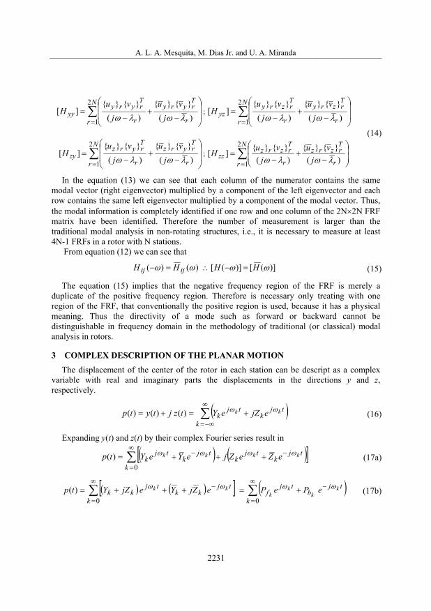
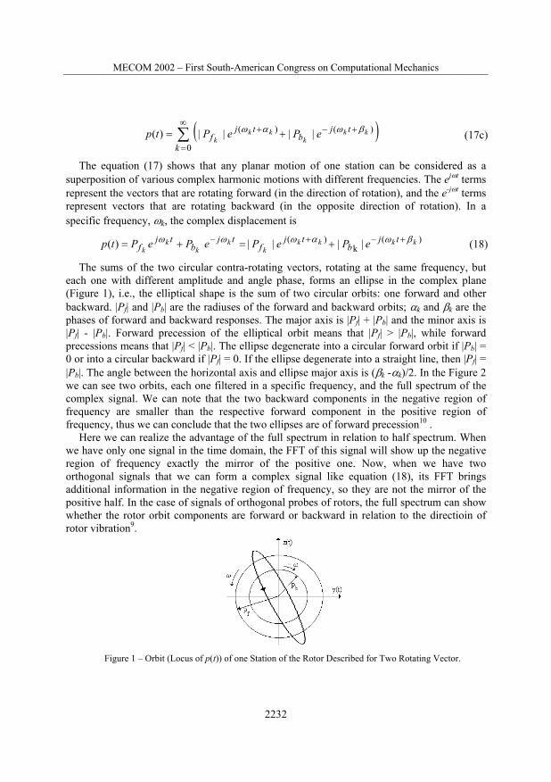
The sums of the two circular contra-rotating vectors, rotating at the same frequency, but each one with different amplitude and angle phase, forms an ellipse in the complex plane (Figure 1), i.e., the elliptical shape is the sum of two circular orbits: one forward and other backward. |Pf| and |Pb| are the radiuses of the forward and backward orbits; k and k are the phases of forward and backward responses. The major axis is |Pf| + |Pb| and the minor axis is |Pf| - |Pb|. Forward precession of the elliptical orbit means that |Pf| > |Pb|, while forward precessions means that |Pf| < |Pb|. The ellipse degenerate into a circular forward orbit if |Pb| = 0 or into a circular backward if |Pf| = 0. If the ellipse degenerate into a straight line, then |Pf| = |Pb|. The angle between the horizontal axis and ellipse major axis is ( k - k)/2. In the Figure 2 we can see two orbits, each one filtered in a specific frequency, and the full spectrum of the complex signal. We can note that the two backward components in the negative region of frequency are smaller than the respective forward component in the positive region of frequency, thus we can conclude that the two ellipses are of forward precession10 .
Here we can realize the advantage of the full spectrum in relation to half spectrum. When we have only one signal in the time domain, the FFT of this signal will show up the negative region of frequency exactly the mirror of the positive one. Now, when we have two orthogonal signals that we can form a complex signal like equation (18), its FFT brings additional information in the negative region of frequency, so they are not the mirror of the positive half. In the case of signals of orthogonal probes of rotors, the full spectrum can show whether the rotor orbit components are forward or backward in relation to the directioin of rotor vibration9.
Figure 1 – Orbit (Locus of p(t)) of one Station of the Rotor Described for Two Rotating Vector.
Figure 2: (a) Orbit of a Rotor Station where the Response is Composed by Two Harmonics; (b) Orbit Filtered
(1X); (c) Orbit Filtered (2X); (d) Full Spectrum.
4 COMPLEX MODAL ANALYSIS As shown in anterior section the planar motion of one station can be described by
)( )()( tzjtytp . Regarding the complex conjugate, the motion can be described, in matricial form, as
)()(
1 1
)()(
tzty
-jj
tptp
)()(
1 1
21
)()(
tptp
j-jtzty
(19)
For N stations, the equation (21) becomes
)}({)}({
][)}({)}({
)}({)}({
][ ][ ][ ][
21
)}({)}({
tptp
Ttzty
tptp
IjI-jII
tzty
(20)
Thus, [T] is defined as the transformation matrix between the real and complex representation and [I] denotes the N N identity matrix. Similarly, the excitation in complex coordinates is written as g(t) = fy(t) + j fz(t). In matricial form it is written as
Substituting equations (22) and (23) into equation (1) leads to
}{][][
}{]][[][
}{]][[][
}{]][[][ 1111
gg
TTpp
TKTpp
TDTpp
TMT (22a)
}{}{][
}{][
}{][
gg
pp
Kpp
Dpp
M aaa (22b)
where [Ma], [Da] and [Ka] are composed by complex elements given by
][ ][
][ ][
][ ][ ][ ][
21
][ ][
][ ][
][ ][][ ][
]][[][][ 1
fb
bf
zzzy
yzyya MM
MM
IjI-jII
MM
MM
I-jIIjI
TMTM
][ ][
][ ][ ][
fb
bfa DD
DDD ;
][ ][
][ ][ ][
fb
bfa KK
KKK
(23)
where
])[]([])[]([][ 2
])[]([])[]([][ 2
zyyzzzyyb
zyyzzzyyf
MMjMMM
MMjMMM (24)
and the same structure is valid for [Df], [Db], [Kf] and [Kb]. The Fourier transforms of )}({ tp , )}({ tp , )}({ tg and )}({ tg are )}({P , )}(ˆ{P ,
)}({G and )}(ˆ{G , respectively. Thus, equation (22b) can be written as
)}(ˆ{
)}({
)}(ˆ{
)}({)]([
)}(ˆ{
)}({][][][2
G
G
P
PB
P
PKDiM aaa (25)
)}(ˆ{
)}({)]([
)}(ˆ{
)}({)]([
)}(ˆ{
)}({ 1G
GH
G
GB
P
P c (26)
)}(ˆ{
)}({
P
P
)}(ˆ{
)}({)]([ )]([
)]([ )]([
ˆˆˆ
ˆ
G
GHH
HH
gpgp
gppg (27)
The sub-matrices in the complex frequency response matrix [H c( )] are called directional frequency response matrices (dFRMs) and its elements are called directional frequency response functions (dFRFs) because they implicitly include directionality. The dFRMs
)]([ and )]([ ˆˆgppg HH relate excitations and responses of the same direction and its elements are referred as “normal dFRFs” (normal forward and normal backward, respectively). The dFRMs )]([ and )]([ ˆˆ gpgp HH relate excitations and responses in opposite directions and its elements are referred as “reverse dFRFs”. According to equations (20), (21) and (27) we obtain the following relations between the FRFs and the dFRFs and substituting the equation above into equation (29) leads to
)]([ )]([
)]([ )]([
ˆˆˆ
ˆ
gpgp
gppg
HH
HH ][
)]([ )]([
)]([ )]([ ][
zz
1 THH
HHT
zy
yzyy (28)
)]([)]([( )]([)]([)]([ 2
)]([)]([( )]([)]([)]([ 2
)]([)]([( )]([)]([)]([ 2
)]([)]([( )]([)]([)]([ 2
ˆˆ
ˆ
ˆ
zyyzzzyygp
zyyzzzyygp
zyyzzzyygp
zyyzzzyypg
HHjHHH
HHjHHH
HHjHHH
HHjHHH
(29)
According to equations (15) and (29), it can be conclude that
)]([)]([ and )]([)]([ ˆˆˆˆ gpgppggp HHHH (30)
Therefore we can conclude that if only positive frequencies are considered, the four sub-matrices are needed to represent the same information as in real modal analysis. However, if negative frequencies are considered too, only two sub-matrices suffice to represent all information. Usually )]([ pgH and )]([ gpH are considered. Thus, considering two-side dFRFs we can rewrite the equation (27) as
)}(ˆ{
)}({)]([ )]([
)}(ˆ{
)}({ˆ G
GHH
P
Pgppg (31)
The equation (22b) can be rewritten in the state space form as
aaaaa QwBwA ][][ (32)
)}({)}({
}{,}{}{
}{,)}({)}({
}{
}{}0{
}{,][- ]0 [
]0[ ][][ ,
][ ][][ ]0[
][ 44
tptp
qqq
wtgtg
F
FQ
KM
BDM
MA
aa
aaa
aa
a
a
aa
aNNa
(33)
The complex matrices [Aa] and [Ba] are indefinite, non-Hermetian in general, resulting in a non-self eigenvalue problem. The eigenvalue problems associated with equation (32) are
The vectors {ua} and {va} are the eigenvectors of the following eigenvalue problems
0)][][][(
0])[][][(2
2
aT
aT
aT
a
aaaa
vKDM
uKDM. (36)
Due the matrices [Aa] and [Ba] (as well as the matrices [Ma], [Da] and [Ka]) are complex and non-Hermetian, we have the most general case of eigenvalue problem. Now, the questions are: the superposition principle still holds here? In other words, the orthogonality properties of the eigenvectors in relation to [Aa] and [Ba] are still valid? The eigenvalues and eigenvectors will appear in conjugate complex? The answers were found in the book of Lancaster10, where the author says that in this case the orthogonality properties and consequently the superposition principle are valid. Lancaster also says that the eigenvalues will appear in complex conjugate pairs but it is not necessarily true for the eigenvectors! It was cited by Joh and Lee5 and repeated in Appendix A that in this case, the right and left eigenvectors corresponding to eigenvalues r and r of the eigenproblem of the equation (36) are
}{}ˆ{
; }{}ˆ{
and }ˆ{}{
};{ }ˆ{}{
}{c
c
c
cr
c
ca
c
car v
vuu
vv
vuu
u (37)
where the symbol (^) denotes that the complex elements in }ˆ{ cu are the same of }{ cu with the exception of the sign of the imaginary part, as we going to see latter. We can note that the eigenvector corresponding to complex conjugate of the eigenvalue is not merely the complex conjugate of the original eigenvector }{ au , but it is composed by the complex conjugate of its terms ( }{ cu and }ˆ{ cu ) when they are in changed position. Thus, in the procedure similar to equation (7) to (11) we obtain the complex frequency response matrix written in terms of modal parameters
According to equations (27) and (38) the dFRM blocks are written as
N
r r
Trcrc
r
Trcrc
pg jvu
jvuH
2
1 )(}ˆ{}ˆ{
)(}{}{][ ;
N
r r
Trcrc
r
Trcrc
gp jvu
jvuH
2
1ˆ )(
}{}ˆ{)(
}ˆ{}{][
N
r r
Trcrc
r
Trcrc
gp jvu
jvuH
2
1ˆ )(
}ˆ{}{)(
}{}ˆ{][ ; N
r r
Trcrc
r
Trcrc
gp jvu
jvuH
2
1ˆˆ )(
}{}{)(
}ˆ{}ˆ{][
(39)
Analyzing the expressions in (39), it can be showed4 that to identify all modal parameters, it is necessary to measure at least one single column (row) of )]([ pgH as well as one single
row (column) of )]([ gpH , which are arbitrarily chosen from the dFRF matrices. It implies that for a anisotropic rotor with N stations, it is necessary measure 2N dFRFs for identification of all modal parameters. The relations between the elements of the modal vectors from both methodology (real and complex) can be found substituting the equation (14) and (39) into equation (29). Using the first relation in (29) we obtain (suppressing the subindex r)
)(}}{{}}{{}}{{}}{{
)(}}{{}}{{}}{{}}{{
)(}ˆ}{ˆ{
)(}}{{
2
jvuvujvuvu
jvuvujvuvu
jvu
jvu
Tyz
Tzy
Tzz
Tyy
Tyz
Tzy
Tzz
TyyT
ccT
cc
(40)
and the equation (40) leads to
}{ }{2
1}{ and }{ }{2
1}{ zyczyc vjvvujuu (41a)
}{ }{2
1}ˆ{ and }{ }{2
1}ˆ{ zyczyc vjvvujuu (41b)
Therefore, according to (41) the vector }ˆ{ cu is different from the vector }{ cu only in respect of the sign of the imaginary part, as already mentioned. The vector }ˆ{ cu is not the complex conjugate of }{ cu because the vectors }{ yu and }{ zu are complex. If the rotor is isotropic its dynamic properties are the same in any direction. Therefore
Rewrite the equations (36) using equations (23), (37) and (43)
}0{}0{
}ˆ{}{
][ ]0[
]0[ ][
][ ]0[
]0[ ][
][ ]0[
]0[ ][2
c
c
f
f
f
f
f
f
uu
K
K
D
D
M
M (44a)
}0{}0{
}ˆ{}{
][ ]0[
]0[ ][
][ ]0[
]0[ ][
][ ]0[
]0[ ][2
c
cT
f
fT
f
fT
f
f
vv
K
K
D
D
M
M (44b)
Thus, it leads to
}0{}{ }{ 0}ˆ{ and }0{}{ }{ 0}ˆ{ zyczyc vjvvujuu (45)
Using equations (45) and (41a) yields
}{ 2}{ 2}{ and }{ 2}{ 2}{ 00 vvvuuu ycyc (46)
Substituting equations (45) and (46) in equation (39) we obtain
N
r r
Trr
pg jvuH
2
1
00)(
}{}{ 2)]([ and 0)]([ gpH (47)
The equation (47) can be rewritten as
N
r
F
rr
Trr
pg jvuH
1
00)(
}{}{ 2][ for and
N
r
B
rr
Trr
pg jvuH
1
00)(
}{}{ 2][ for < (48)
The over scripts F and B denote forward and backward modes. As shown in (48), forward (backward) modes are excited by only forward (backward) excitations, i.e., the forward (backward) modes appear in only the positive (negative) frequency region. If some anisotropy of bearings are permitted, backward (forward) modes start to be excited by forward (backward) rotating excitations. The magnitude of the dFRF of forward (backward) modes in the negative (positive) frequency region indicates the strength of the system anisotropy. Even if the anisotropy of the system is great, the magnitudes of the FRF of the forward (backward) modes in positive frequency region are greater (smaller) or equal than those in negative frequency region6. It is the same idea as shown in section 3.
5 CONSIDERATIONS ABOUT NUMERICAL IMPLEMENTATION One of the objectives of this work was to develop a finite element code, which could use both formulations real and complex. The matrices of the finite elements implemented in the
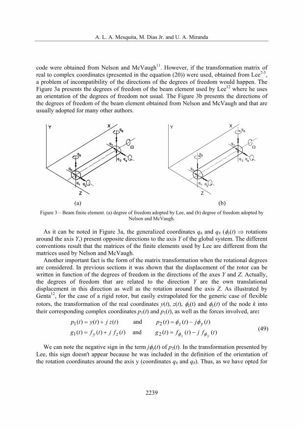
code were obtained from Nelson and McVaugh11. However, if the transformation matrix of real to complex coordinates (presented in the equation (20)) were used, obtained from Lee2-5, a problem of incompatibility of the directions of the degrees of freedom would happen. The Figure 3a presents the degrees of freedom of the beam element used by Lee12 where he uses an orientation of the degrees of freedom not usual. The Figure 3b presents the directions of the degrees of freedom of the beam element obtained from Nelson and McVaugh and that are usually adopted for many other authors.
q
q
q
q
q
q
q
q3 4
8
7
6
5
1 2
XY
Z
q
q
q
q
q
q
q
q3 4
8
7
6
5
1 2
XY
Z
q
q
q
q
q
q
q
q3 4
8
7
6
5
1 2
XY
Z
(a) (b) Figure 3 – Beam finite element. (a) degree of freedom adopted by Lee, and (b) degree of freedom adopted by
Nelson and McVaugh.
As it can be noted in Figure 3a, the generalized coordinates q6 and q8 ( y(t) rotations around the axis Y,) present opposite directions to the axis Y of the global system. The different conventions result that the matrices of the finite elements used by Lee are different from the matrices used by Nelson and McVaugh. Another important fact is the form of the matrix transformation when the rotational degrees are considered. In previous sections it was shown that the displacement of the rotor can be written in function of the degrees of freedom in the directions of the axes Y and Z. Actually, the degrees of freedom that are related to the direction Y are the own translational displacement in this direction as well as the rotation around the axis Z. As illustrated by Genta12, for the case of a rigid rotor, but easily extrapolated for the generic case of flexible rotors, the transformation of the real coordinates y(t), z(t), z(t) and y(t) of the node k into their corresponding complex coordinates p1(t) and p1(t), as well as the forces involved, are:
)( )()( and )( )()(
)()()( and )( )()(
21
21
tfjtftgtfjtftg
tjttptzjtytp
yzzy
yz (49)
We can note the negative sign in the term j y(t) of p2(t). In the transformation presented by Lee, this sign doesn't appear because he was included in the definition of the orientation of the rotation coordinates around the axis y (coordinates q6 and q8). Thus, as we have opted for
maintaining Nelson and McVaugh's formulation, it was necessary to modify the coordinates matrix transformation proposed by Lee. Therefore, the transformation of the real degrees of freedom for complex ones becomes
This alteration resulted that all modeling of the rotor could be accomplished independently of the type of coordinates (real or complex) chosen to analyze the behavior of the rotating system, as it was the initial objective. Considering all nodes of the finite element model and the new matrix transformation, we can rewrite the equation (22a) as
}{][][
}{]][[][
}{]][[][
}{]][[][ 1111
gg
TTpp
TKTpp
TDTpp
TMT nnnnnnnn (52a)
}{}{][
}{][
}{][
gg
pp
Kpp
Dpp
M nnn (52b)
where [Mn] is composed by complex elements given by
and remembering that ][ bnM and ][ fnM are the complex conjugate of ][ bnM and ][ fnM , respectively. Comparing equations (23) and equation (53c) we can note that both equations for the mass matrix have the same structure. The expressions of the elements of [Dn] and [Kn] and are found in the same way of [Mn]. In similar manner, the FRF matrix is now written as
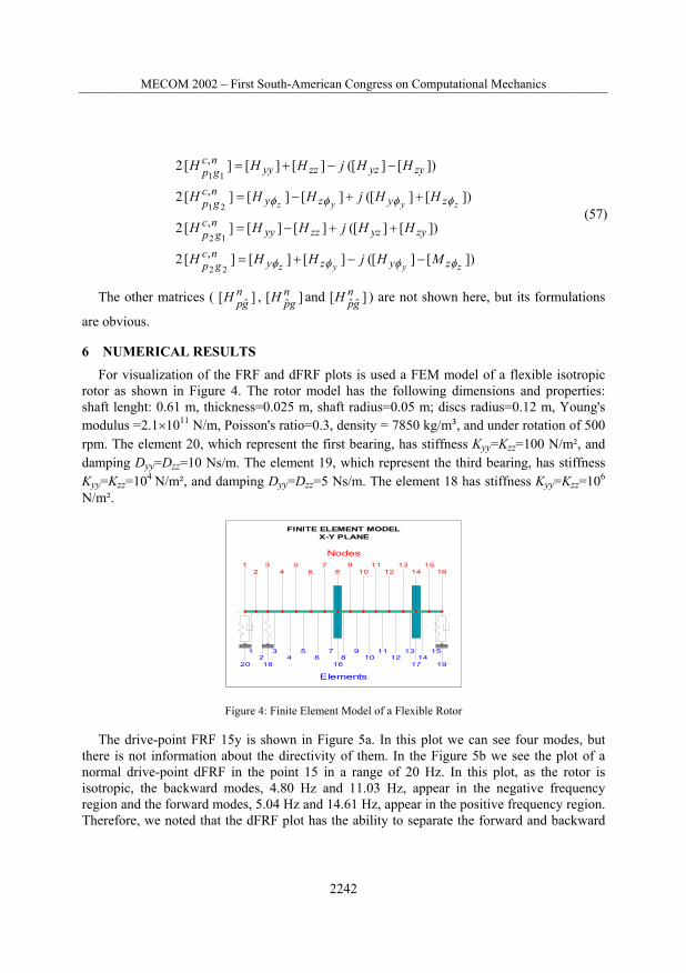
6 NUMERICAL RESULTS For visualization of the FRF and dFRF plots is used a FEM model of a flexible isotropic rotor as shown in Figure 4. The rotor model has the following dimensions and properties: shaft lenght: 0.61 m, thickness=0.025 m, shaft radius=0.05 m; discs radius=0.12 m, Young's modulus =2.1 1011 N/m, Poisson's ratio=0.3, density = 7850 kg/m³, and under rotation of 500 rpm. The element 20, which represent the first bearing, has stiffness Kyy=Kzz=100 N/m², and damping Dyy=Dzz=10 Ns/m. The element 19, which represent the third bearing, has stiffness Kyy=Kzz=104 N/m², and damping Dyy=Dzz=5 Ns/m. The element 18 has stiffness Kyy=Kzz=106
N/m².
Nodes
Elements
FINITE ELEMENT MODELX-Y PLANE
12
1
3
2
4
3
5
4
6
5
7
6
8
7
9
8
10
9
11
10
12
11
13
12
14
13
15
14
16
15
16 1718 1920
Figure 4: Finite Element Model of a Flexible Rotor
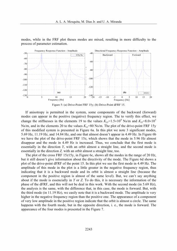
The drive-point FRF 15y is shown in Figure 5a. In this plot we can see four modes, but there is not information about the directivity of them. In the Figure 5b we see the plot of a normal drive-point dFRF in the point 15 in a range of 20 Hz. In this plot, as the rotor is isotropic, the backward modes, 4.80 Hz and 11.03 Hz, appear in the negative frequency region and the forward modes, 5.04 Hz and 14.61 Hz, appear in the positive frequency region. Therefore, we noted that the dFRF plot has the ability to separate the forward and backward
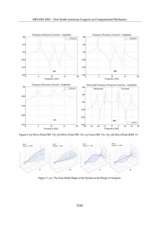
If anisotropy is permitted in the system, some components of the backward (forward) modes can appear in the positive (negative) frequency region. The to verify this effect, we change the stiffnesses in the elements 19 to the values Kyy=1.5 104 Ns/m and Kzz=8.0 103 Ns/m, and in the elements 20 to the values Kzz=80 Ns/m. The plot of the drive-point FRF 15y of this modified system is presented in Figure 6a. In this plot we note 3 significant modes, 5.69 Hz, 11.19 Hz, and 14.84 Hz, and one that almost doesn’t appear in 4.49 Hz. In Figure 6b we have the plot of the drive-point FRF 15z, which shows that the mode in 5.96 Hz almost disappear and the mode in 4.49 Hz is increased. Thus, we conclude that the first mode is essentially in the direction Y, with an orbit almost a straight line, and the second mode is essentially in the direction Z, with an orbit almost a straight line, too. The plot of the cross FRF 15z15y, in Figure 6c, shows all the modes in the range of 20 Hz, but it still doesn’t give information about the directivity of the mode. The Figure 6d shows a plot of the drive-point dFRF of the point 15. In this plot we see the first mode in 4.49 Hz. The amplitude of this mode in the plot is a little greater in the negative frequency region, thus indicating that it is a backward mode and its orbit is almost a straight line (because the component in the positive region is almost of the same level). But, we can’t say anything about if the mode is essencially in Y or Z. To do this, it is necessary the information of the phase of the dFRF, and this will not be deal in this work. With the second mode (in 5.69 Hz), the analysis is the same, with the difference that, in this case, the mode is forward. But, with the third mode (in 11.19 Hz), we easily note that it is a backward mode. The amplitude is very higher in the negative frequency region than the positive one. The appearance of a component of very low amplitude in the positive region indicate that the orbit is almost a circle. The same happenn with the fourth mode, but in the opposite direction, i. e., the mode is forward. The appareance of the four modes is presented in the Figure 7.
7 CONCLUDING REMARKS In this paper the mathematical theory of frequency response function (FRF), used in
traditional modal analysis in rotors, and the directional frequency response function (dFRF) used in the complex modal analysis are fully described. In addition, numerical implementation aspects are discussed in order to have both the methodologies in only one computational program FEM based.
In the analysis of the numerical simulation of isotropic and anisotropic rotors, it was verified that in the plot of the dFRF, the directivity of the rotating modes could be identified, and depending on the characteristics of the system, the forward and backward modes can be completely separated in the two sided dFRF.
ACKNOWLEDGEMENTS The authors would like to thank the Fundação de Amparo à Pesquisa do Estado de São Paulo (FAPESP) and the Coordenação de Aperfeiçoamento de Pessoal de Nível Superior (CAPES) for the financial support of this project.
10. REFERENCES [1] P.J. Rogers and D.J. Ewins, “Modal Testing of an Operating Rotor System Using a
Structural Dynamics Approach”, Proceedings of the 7th IMAC, 466-473 (1989). [2] C.W. Lee, “A New Test Theory in Rotating Machinery”, Proceedings of the 8th IMAC,
148-154 (1990). [3] C.W. Lee, “Complex Modal Testing Theory for Rotating Machinery”, Mechanical
System and Signal Processing, 5(2), 119-137 (1991). [4] C.W. Lee and Y.D. Joh, “Theory and Excitation Methods and Estimation of Frequency
Response Function in Complex Modal Testing of Rotating Machinery”, Mechanical System and Signal Processing, 7(1), 57-74 (1993).
[5] Y.D. Joh and C.W. Lee, “Excitation Methods and Modal Parameter Identification in Complex Modal Testing of Rotating Machinery”, Modal Analysis: The International Journal of Analytical and Experimental Modal Analysis, 8(3), 179-203 (1993).
[6] Y.G. Jei and Y.J. Kim, “Modal Testing Theory of Rotor-Bearing System”, Trans. of the ASME, Journal of Vibration and Acoustics, 115, 165-176 (1993).
[7] C. Kessler and J. Kim, “Complex Modal Analysis and Interpretation for Rotating Machinery”, Proceedings of the 16th Int. Modal Analysis Conf., 782-787 (1998).
[8] C. Kessler and J. Kim, “Complex Modal Analysis Superposition for Rotating Machinery”, Proc. of the 17th Int. Modal Analysis Conf., 1930-1937 (1999).
[9] P. Goldman and A. Muszynska, “Application of Full Spectrum to Rotating Machinery Diagnostics”, Orbit Magazine, First Quarter, 17 – 21 (1999)
[10] P. Lancaster, Lambda-Matrices and Vibrating Systems, Pergamon Press, (1966). [11] H.D. Nelson and J. M. McVaugh, “The Dynamics of Rotor-Bearing System Using Finite
Element”, Journal of Engineering for Industry, 593-600, (1976) [12] C.W. Lee and Y.G. Jei, “Modal Analysis of a Continuous Rotor-Bearing System”,
Journal of Sound and Vibration, 126, 345-361, (1988) [13] G. Genta, “Vibration of Structures and Machines”, Spring – Verlag, 3rd Edition, (1999).
APPENDIX A – EIGENVALUES AND EIGENVECTORS OF A SPECIAL COMPLEX MATRICES FORM Let the following eigenvalue problem where the vector {u} is the eigenvector corresponding to eigenvalue .
0])[][][( 2 uKDM (A.1)
If the matrices [M], [D] and [K] are real (symmetrical or not) it is well known that the eigenvalues and the eigenvectors appear in complex conjugate pairs. Now, if the matrices are complex, but in a special form as
}0{}0{
}{}{
]][[]][[
]][[]][[
]][[]][[
2
1
12
21
12
21
12
212uu
KKKK
DDDD
MMMM
(A.2)
Here, the vector {{u1}{u2}}T is the eigenvector associated with the eigenvalue . We want to know what is the eigenvector associated with the complex conjugate of . Ir order to answer this question, we can decompose the equation (A.2) as
}0{}]{[}]{[}]{[}]{[}]{[}]{[
}0{}]{[}]{[}]{[}]{[}]{[}]{[
2112211221122
2211221122112
uKuKuDuDuMuM
uKuKuDuDuMuM (A.3)
If we transpose the both equations above, we have
}0{}]{[}]{[}]{[}]{[}]{[}]{[
}0{}]{[}]{[}]{[}]{[}]{[}]{[
2112211221122
2211221122112
uKuKuDuDuMuM
uKuKuDuDuMuM (A.4)
}0{}0{
}{}{
]][[]][[
]][[]][[
]][[]][[
2
1
12
21
12
21
12
212uu
KKKK
DDDD
MMMM
(A.5)
If we invert the order of the rows in equation (A.5) and changing the order of the columns of the matrices, as well as the position of the terms of the eigenvector, we obtain
}0{}0{
}{}{
]][[]][[
]][[]][[
]][[]][[
1
2
12
21
12
21
12
212uu
KKKK
DDDD
MMMM
(A.6)
Therefore we can conclude by inspection that the eigenvector corresponding to the complex conjugate of the eigenvalue in this problem is not the complex conjugate of the original vector,, as we can see in equations (A.2) and (A.6).