A Comparison of Different Face Recognition Algorithms

Yi-Shin Liu Wai-Seng Ng Chun-Wei LiuNational Taiwan University

{sitrke,markng,dreamway}@cmlab.csie.ntu.edu.tw

Abstract

We make a comparison of five different face recognitionalgorithms. Four existed algorithm and a new EnsembleVoting Algorithm were be implemented. The algorithmstraining on a data set with 1815 faces, registering on agallery set with 1027 faces, and test on four different probesets. This paper will detail the parameter tuning process,and report the testing result via receiver operating charac-teristic (ROC) curve and verification accuracy.

1. Introduction

Face Recognition has been researched for several years,different type of methods tried to solve two major problemsin this area: face identification , and face verification. Faceidentification try to indicate the identity of a visitor. Fisher-faces [2] and Local Binary Patterns (LBP) [1] perform wellin this function; In the other hands, face verification, whichtry to verify if a visitor is truly as his claim. Facial TraitCode (FTC) [4] and the Ensemble Voting Algorithm (EVA)perform well. The Eigenfaces [5] will be mention as a ref-erence. We briefly introduce these methods below.

1.1. Related Works

Principle component analysis (PCA) is widely usedfor dimensionality reduction, Turk and Pentland introduceEigenfaces in 1991 [5]. By this method, the dimensional-ity of a face model can be reduced from image pixel size toseveral principle basis, the basis may encode sufficient in-formation about the face. However, it is designed in a wayto best preserve data in the embedding space, and conse-quently cannot promise good discriminating capability.

Linear discriminant analysis (LDA) is also used for di-mensionality reduction, and it provide a good discriminat-ing capability. Fisherfaces [2] improve the face recognitionsystem, but the drawback of this method is it can not per-form well in face verification.

LBP is a powerful method to solve face recognition prob-lem, it is efficient and also easy to implement. The draw-

back is it is hard to determine a verification threshold, whichmean the boundary between imposter and guest is hard todetermine in chi square distance matrix space.

FTC has good performance on verification, its distancematrix in discrete integer space helping us tuning verifica-tion easier than other methods. In contrast to setting thethreshold, tuning the parameters of FTC are really compli-cated and time-consuming, we do lots of efforts on this al-gorithm. Thus, tuning FTC is the bottle neck of the project.

1.2. Our Approach

Ensemble Voting Algorithm (EVA) tries to gather differ-ent opinions of face recognition algorithms, and votes fora common idea for final decision. The algorithm achieve95% accuracy in a random sample 20 faces set containedimposter and gallery face.

We will introduce the methods, and detail the parametertuning process of five algorithms in section 2., most of con-tent will focus on FTC’s tuning. And then we discuss theperformance on different algorithms, the ROC curve andhighest precision will be reported in section 3.. In the endof the paper, we will discuss the whole system and make aconclusion.

2. Implementation and TuningWe describe the implementation and parameter tuning

process in this section. Each section will briefly explain theapproach of implementation, and show a figure illustratedthe relation ship between accuracy and different types ofparameters. We decide the parameter for testing is based onoverall performance in different data sets.

2.1. Eigenfaces

Eigenfaces was proposed by Turk and Pentland in1991 [5]. The idea takes a face as a column vector ofpixels x, where the length of the vector d represents theproduct of patch’s width and height. Suppose we haven′s faces x1, x2, ..., xn, denote the faces as a matrix X ={x1, x2, ..., xn}. We training the Eigenfaces model of thesedata in the following steps:

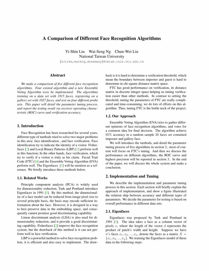
Figure 1. Accuracy of PCA in different parameters.

1. Compute the scatter matrix S = (X −M)(X −M)T ,where M is a matrix that each column represents themean vector µ of x1, x2, ..., xn.

2. Solve the eigenvalues of S, pick the eigenvectors ofk′s largest eigenvalue as the basis of X .

The output model is a matrix E which concatenates k′seigenvectors. The model is used to linearly project an in-put vector x as y = ETx.

Clearly, the tuning factors are k, the dimensionality ofprojected vector y; and also the input image pixels d. Weplot the dimensionality-accuracy curve in Figure 1 to seethe performance.

As our respect, too large patches are not useful in PCAcase. Because we only have 1815 faces, but the data wouldseparated in 8000 dimensionalities if we used 80∗100 patchsize. Therefore a curse of dimensionality effect is be re-spected. The accuracy of PCA will be limited by increasingthe dimensionality after projected, because the last eigen-vector is not as importance as first one.

We weighted average the accuracy of different probesets. They are 294 images in the neutral , 111 in the illu-mination, 246 in the expression, and 53 in the pose facesdata set. The best average performance in the pose sets isachieved by d = 64 ∗ 80 and k = 300, we choose them fortesting.

2.2. Fisherfaces

Fisherfaces was proposed by Belhumeur et al. in1997 [2]. The idea is same as Eigenfaces, but using discrim-inable linear projection model. Therefore, the scatter matrixis divided into the between-class scatter matrix which be de-fined as

SB =c∑

i=1

Ni(µi − µ)(µi − µ)T

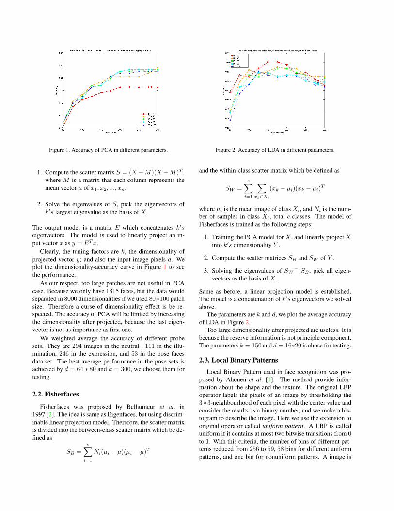
Figure 2. Accuracy of LDA in different parameters.

and the within-class scatter matrix which be defined as

SW =c∑

i=1

∑xk∈Xi

(xk − µi)(xk − µi)T

where µi is the mean image of class Xi, and Ni is the num-ber of samples in class Xi, total c classes. The model ofFisherfaces is trained as the following steps:

1. Training the PCA model for X , and linearly project Xinto k′s dimensionality Y .

2. Compute the scatter matrices SB and SW of Y .

3. Solving the eigenvalues of SW−1SB , pick all eigen-

vectors as the basis of X .

Same as before, a linear projection model is established.The model is a concatenation of k′s eigenvectors we solvedabove.

The parameters are k and d, we plot the average accuracyof LDA in Figure 2.

Too large dimensionality after projected are useless. It isbecause the reserve information is not principle component.The parameters k = 150 and d = 16∗20 is chose for testing.

2.3. Local Binary Patterns

Local Binary Pattern used in face recognition was pro-posed by Ahonen et al. [1]. The method provide infor-mation about the shape and the texture. The original LBPoperator labels the pixels of an image by thresholding the3 ∗ 3-neighbourhood of each pixel with the center value andconsider the results as a binary number, and we make a his-togram to describe the image. Here we use the extension tooriginal operator called uniform pattern. A LBP is calleduniform if it contains at most two bitwise transitions from 0to 1. With this criteria, the number of bins of different pat-terns reduced from 256 to 59, 58 bins for different uniformpatterns, and one bin for nonuniform patterns. A image is

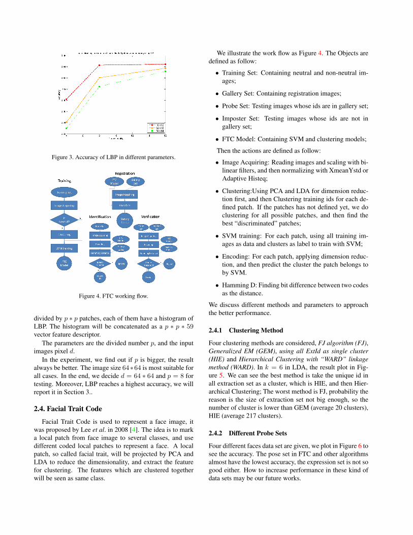
Figure 3. Accuracy of LBP in different parameters.

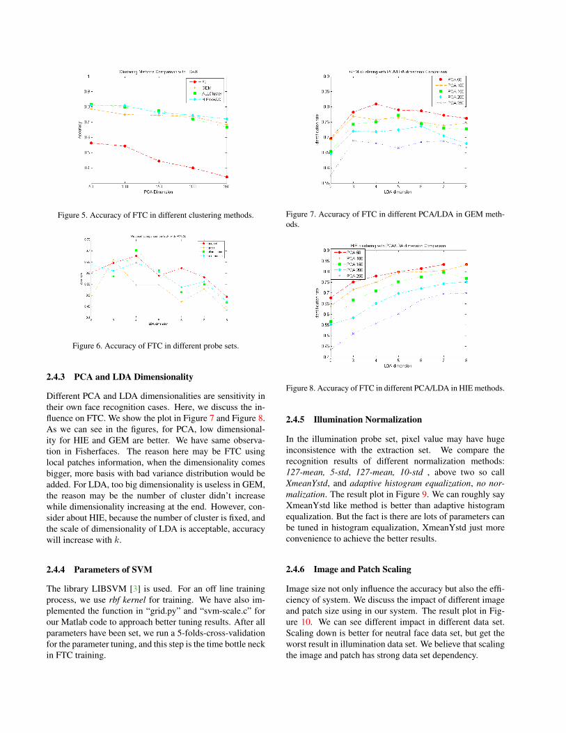
Figure 4. FTC working flow.

divided by p ∗ p patches, each of them have a histogram ofLBP. The histogram will be concatenated as a p ∗ p ∗ 59vector feature descriptor.

The parameters are the divided number p, and the inputimages pixel d.

In the experiment, we find out if p is bigger, the resultalways be better. The image size 64∗64 is most suitable forall cases. In the end, we decide d = 64 ∗ 64 and p = 8 fortesting. Moreover, LBP reaches a highest accuracy, we willreport it in Section 3..

2.4. Facial Trait Code

Facial Trait Code is used to represent a face image, itwas proposed by Lee et al. in 2008 [4]. The idea is to marka local patch from face image to several classes, and usedifferent coded local patches to represent a face. A localpatch, so called facial trait, will be projected by PCA andLDA to reduce the dimensionality, and extract the featurefor clustering. The features which are clustered togetherwill be seen as same class.

We illustrate the work flow as Figure 4. The Objects aredefined as follow:

• Training Set: Containing neutral and non-neutral im-ages;

• Gallery Set: Containing registration images;

• Probe Set: Testing images whose ids are in gallery set;

• Imposter Set: Testing images whose ids are not ingallery set;

• FTC Model: Containing SVM and clustering models;

Then the actions are defined as follow:

• Image Acquiring: Reading images and scaling with bi-linear filters, and then normalizing with XmeanYstd orAdaptive Histeq;

• Clustering:Using PCA and LDA for dimension reduc-tion first, and then Clustering training ids for each de-fined patch. If the patches has not defined yet, we doclustering for all possible patches, and then find thebest “discriminated” patches;

• SVM training: For each patch, using all training im-ages as data and clusters as label to train with SVM;

• Encoding: For each patch, applying dimension reduc-tion, and then predict the cluster the patch belongs toby SVM.

• Hamming D: Finding bit difference between two codesas the distance.

We discuss different methods and parameters to approachthe better performance.

2.4.1 Clustering Method

Four clustering methods are considered, FJ algorithm (FJ),Generalized EM (GEM), using all ExtId as single cluster(HIE) and Hierarchical Clustering with “WARD” linkagemethod (WARD). In k = 6 in LDA, the result plot in Fig-ure 5. We can see the best method is take the unique id inall extraction set as a cluster, which is HIE, and then Hier-archical Clustering; The worst method is FJ, probability thereason is the size of extraction set not big enough, so thenumber of cluster is lower than GEM (average 20 clusters),HIE (average 217 clusters).

2.4.2 Different Probe Sets

Four different faces data set are given, we plot in Figure 6 tosee the accuracy. The pose set in FTC and other algorithmsalmost have the lowest accuracy, the expression set is not sogood either. How to increase performance in these kind ofdata sets may be our future works.

Figure 5. Accuracy of FTC in different clustering methods.

Figure 6. Accuracy of FTC in different probe sets.

2.4.3 PCA and LDA Dimensionality

Different PCA and LDA dimensionalities are sensitivity intheir own face recognition cases. Here, we discuss the in-fluence on FTC. We show the plot in Figure 7 and Figure 8.As we can see in the figures, for PCA, low dimensional-ity for HIE and GEM are better. We have same observa-tion in Fisherfaces. The reason here may be FTC usinglocal patches information, when the dimensionality comesbigger, more basis with bad variance distribution would beadded. For LDA, too big dimensionality is useless in GEM,the reason may be the number of cluster didn’t increasewhile dimensionality increasing at the end. However, con-sider about HIE, because the number of cluster is fixed, andthe scale of dimensionality of LDA is acceptable, accuracywill increase with k.

2.4.4 Parameters of SVM

The library LIBSVM [3] is used. For an off line trainingprocess, we use rbf kernel for training. We have also im-plemented the function in “grid.py” and “svm-scale.c” forour Matlab code to approach better tuning results. After allparameters have been set, we run a 5-folds-cross-validationfor the parameter tuning, and this step is the time bottle neckin FTC training.

Figure 7. Accuracy of FTC in different PCA/LDA in GEM meth-ods.

Figure 8. Accuracy of FTC in different PCA/LDA in HIE methods.

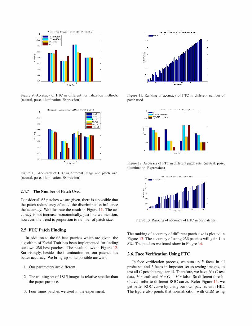
2.4.5 Illumination Normalization

In the illumination probe set, pixel value may have hugeinconsistence with the extraction set. We compare therecognition results of different normalization methods:127-mean, 5-std, 127-mean, 10-std , above two so callXmeanYstd, and adaptive histogram equalization, no nor-malization. The result plot in Figure 9. We can roughly sayXmeanYstd like method is better than adaptive histogramequalization. But the fact is there are lots of parameters canbe tuned in histogram equalization, XmeanYstd just moreconvenience to achieve the better results.

2.4.6 Image and Patch Scaling

Image size not only influence the accuracy but also the effi-ciency of system. We discuss the impact of different imageand patch size using in our system. The result plot in Fig-ure 10. We can see different impact in different data set.Scaling down is better for neutral face data set, but get theworst result in illumination data set. We believe that scalingthe image and patch has strong data set dependency.

Figure 9. Accuracy of FTC in different normalization methods.(neutral, pose, illumination, Expression)

Figure 10. Accuracy of FTC in different image and patch size.(neutral, pose, illumination, Expression)

2.4.7 The Number of Patch Used

Consider all 63 patches we are given, there is a possible thatthe patch redundancy effected the discrimination influencethe accuracy. We illustrate the result in Figure 11. The ac-curacy is not increase monotonically, just like we mention,however, the trend is proportion to number of patch size.

2.5. FTC Patch Finding

In addition to the 63 best patches which are given, thealgorithm of Facial Trait has been implemented for findingour own 256 best patches. The result shows in Figure 12.Surprisingly, besides the illumination set, our patches hasbetter accuracy. We bring up some possible answers.

1. Our parameters are different.

2. The training set of 1815 images is relative smaller thanthe paper purpose.

3. Four times patches we used in the experiment.

Figure 11. Ranking of accuracy of FTC in different number ofpatch used.

Figure 12. Accuracy of FTC in different patch sets. (neutral, pose,illumination, Expression)

Figure 13. Ranking of accuracy of FTC in our patches.

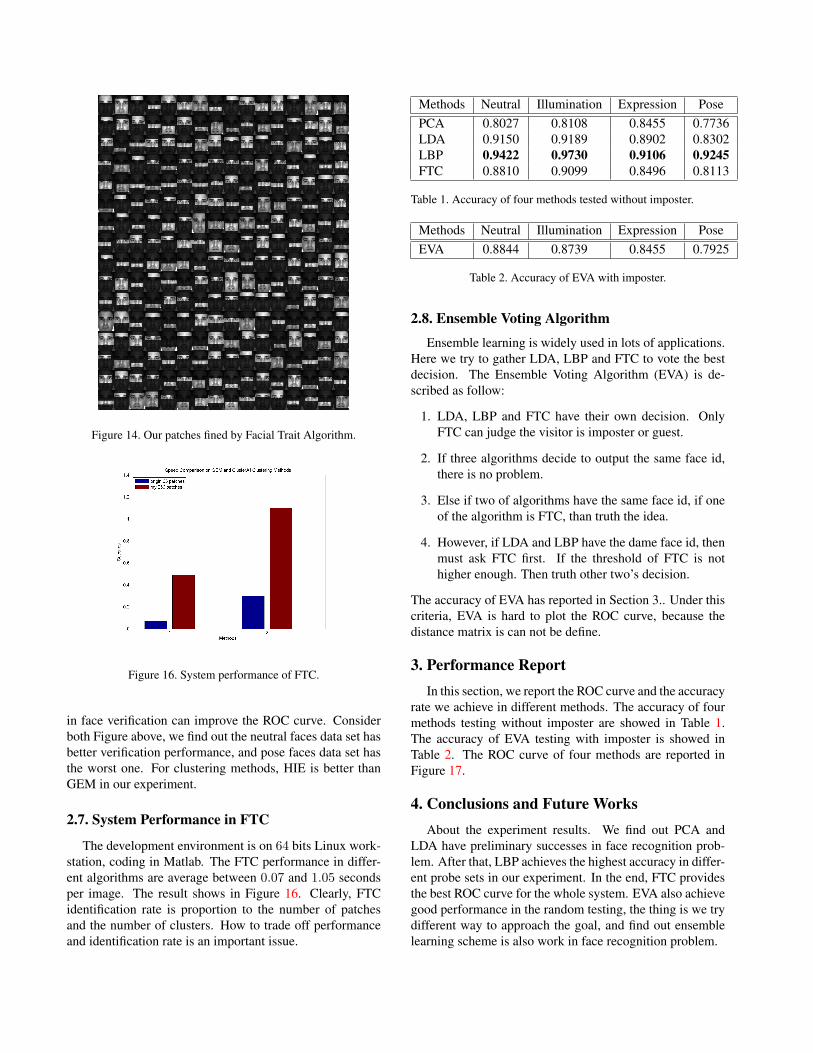
The ranking of accuracy of different patch size is plotted inFigure 13. The accuracy of using 256 patches will gain 1 to3%. The patches we found show in Fiugre 14.

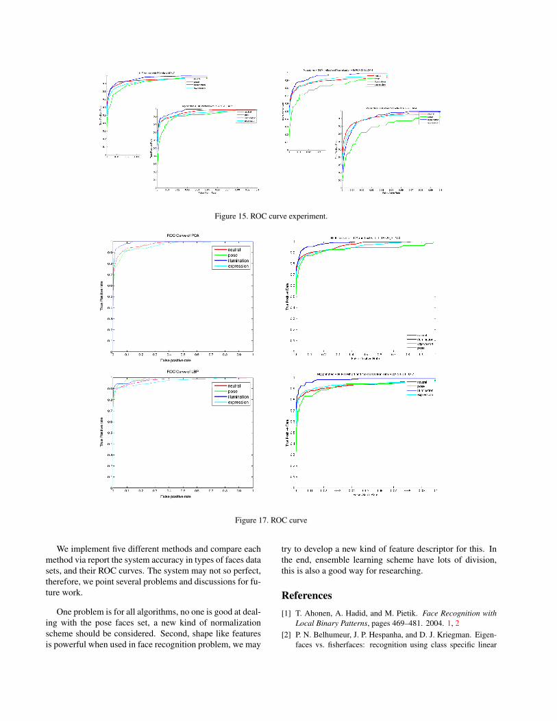
2.6. Face Verification Using FTC

In face verification process, we sum up P faces in allprobe set and I faces in imposter set as testing images, totest allG possible register id. Therefore, we haveN ∗G testdata, P ′s truth and N ∗G− P ′s false. So different thresh-old can refer to different ROC curve. Refer Figure 15, weget better ROC curve by using our own patches with HIE.The figure also points that normalization with GEM using

Figure 14. Our patches fined by Facial Trait Algorithm.

Figure 16. System performance of FTC.

in face verification can improve the ROC curve. Considerboth Figure above, we find out the neutral faces data set hasbetter verification performance, and pose faces data set hasthe worst one. For clustering methods, HIE is better thanGEM in our experiment.

2.7. System Performance in FTC

The development environment is on 64 bits Linux work-station, coding in Matlab. The FTC performance in differ-ent algorithms are average between 0.07 and 1.05 secondsper image. The result shows in Figure 16. Clearly, FTCidentification rate is proportion to the number of patchesand the number of clusters. How to trade off performanceand identification rate is an important issue.

Methods Neutral Illumination Expression PosePCA 0.8027 0.8108 0.8455 0.7736LDA 0.9150 0.9189 0.8902 0.8302LBP 0.9422 0.9730 0.9106 0.9245FTC 0.8810 0.9099 0.8496 0.8113

Table 1. Accuracy of four methods tested without imposter.

Methods Neutral Illumination Expression PoseEVA 0.8844 0.8739 0.8455 0.7925

Table 2. Accuracy of EVA with imposter.

2.8. Ensemble Voting Algorithm

Ensemble learning is widely used in lots of applications.Here we try to gather LDA, LBP and FTC to vote the bestdecision. The Ensemble Voting Algorithm (EVA) is de-scribed as follow:

1. LDA, LBP and FTC have their own decision. OnlyFTC can judge the visitor is imposter or guest.

2. If three algorithms decide to output the same face id,there is no problem.

3. Else if two of algorithms have the same face id, if oneof the algorithm is FTC, than truth the idea.

4. However, if LDA and LBP have the dame face id, thenmust ask FTC first. If the threshold of FTC is nothigher enough. Then truth other two’s decision.

The accuracy of EVA has reported in Section 3.. Under thiscriteria, EVA is hard to plot the ROC curve, because thedistance matrix is can not be define.

3. Performance ReportIn this section, we report the ROC curve and the accuracy

rate we achieve in different methods. The accuracy of fourmethods testing without imposter are showed in Table 1.The accuracy of EVA testing with imposter is showed inTable 2. The ROC curve of four methods are reported inFigure 17.

4. Conclusions and Future WorksAbout the experiment results. We find out PCA and

LDA have preliminary successes in face recognition prob-lem. After that, LBP achieves the highest accuracy in differ-ent probe sets in our experiment. In the end, FTC providesthe best ROC curve for the whole system. EVA also achievegood performance in the random testing, the thing is we trydifferent way to approach the goal, and find out ensemblelearning scheme is also work in face recognition problem.

Figure 15. ROC curve experiment.

Figure 17. ROC curve

We implement five different methods and compare eachmethod via report the system accuracy in types of faces datasets, and their ROC curves. The system may not so perfect,therefore, we point several problems and discussions for fu-ture work.

One problem is for all algorithms, no one is good at deal-ing with the pose faces set, a new kind of normalizationscheme should be considered. Second, shape like featuresis powerful when used in face recognition problem, we may

try to develop a new kind of feature descriptor for this. Inthe end, ensemble learning scheme have lots of division,this is also a good way for researching.

References[1] T. Ahonen, A. Hadid, and M. Pietik. Face Recognition with

Local Binary Patterns, pages 469–481. 2004. 1, 2[2] P. N. Belhumeur, J. P. Hespanha, and D. J. Kriegman. Eigen-

faces vs. fisherfaces: recognition using class specific linear

projection. Pattern Analysis and Machine Intelligence, IEEETransactions on, 19(7):711–720, 1997. 1, 2

[3] C.-C. Chang and C.-J. Lin. LIBSVM: a library for supportvector machines, 2001. Software available at http://www.csie.ntu.edu.tw/˜cjlin/libsvm. 4

[4] P.-H. Lee, G.-S. Hsu, T. Chen, and Y.-P. Hung. Facial traitcode and its application to face recognition. In ISVC ’08: Pro-ceedings of the 4th International Symposium on Advances inVisual Computing, Part II, pages 317–328, Berlin, Heidelberg,2008. Springer-Verlag. 1, 3

[5] M. A. Turk and A. P. Pentland. Face recognition using eigen-faces. pages 586–591, 1991. 1