A COMPARISON OF METHODS IN FULLY NONLINEARBOUNDARY ELEMENT NUMERICAL WAVE TANK

DEVELOPMENT

J.C. HARRIS∗, E. DOMBRE∗, M. BENOIT∗, S.T. GRILLI∗∗

* Laboratoire d’Hydraulique Saint-Venant, Universite Paris-Est, Chatou, France

** Dept. of Ocean Engineering, University of Rhode Island, Narragansett, RI 02882, USA

jeffrey-externe.harris@edf.fr

Summary

We present the development and validation of an efficient numerical wave tank (NWT)solving fully nonlinear potential flow (FNPF) equations. This approach is based on avariation of the 3D-MII (mid-interval interpolation) boundary element method (BEM),with mixed Eulerian-Lagrangian (MEL) explicit time integration, of Grilli et al., whichhas been successful at modeling many phenomena, including landslide-generated tsunami,rogue waves, and the initiation of wave breaking over slopes. The MEL time integrationis based on a second-order Taylor series expansion, requiring to compute high order timeand space derivatives. In order to solve wave-structure interaction problems with complexgeometries, we reformulate the model to use a 3D unstructured triangular mesh, buildingon earlier work, but presently only working with linear elements. The added flexibilityof arbitrary meshes is demonstrated by modeling the longitudinal forces on a trunca-ted (surface-piercing) vertical cylinder, comparing to theory and experiment. In order toimprove the computational efficiency of the BEM, we apply the fast multipole method(FMM), in the context of the new unstructured mesh. A detailed study of the resultingcomputational time shows both the efficiency of the earlier 3D-MII approach and theproposed one, and also what is necessary to scale such results up to larger grids.

I – Introduction

Potential flow theory, which assumes irrotational (and thus inviscid) flows, has beenvery successful for modeling non-breaking water waves and wave-structure interactions,and is a standard tool in ocean engineering. Generally, at a given resolution, potential flowmodels have much less artificial dissipation than Navier-Stokes models, resulting in fas-ter and more accurate results. Typically, in potential flow models, the boundary elementmethod (BEM) is used to compute the solution for flows around ships and offshore struc-tures. Numerous industrial wave models have been developed under this assumption, e.g.,WAMIT [26], AQUAPLUS [5], and AEGIR [24]. Current numerical wave tanks (NWTs)based on the BEM have relatively similar approaches, as reviewed by Tanizawa [37]. Thetime-domain solution of fully nonlinear potential flow (FNPF) equations, however, re-quires solving an elliptic problem (Laplace’s equation) with the BEM at each time step,which represents the biggest limitation of the method in terms of computational time,

1

even for moderately large grids ; this is by contrast with standard linear frequency do-main solutions (e.g., WAMIT) where only one BEM solution is performed per frequency.In the traditional BEM, for N degrees of freedom (DOFs), the assembly of a dense systemof linear equations takes both a O(N2) computational effort and computer memory. Com-bined with a time step ∆t that must be proportional to the grid resolution ∆x (basedon a constant mesh Courant number), BEM approaches for wave models have a CPUtime that is O[(∆x)5], which is a severe limitation for fully nonlinear NWT development.It can often be sufficient to assume weak nonlinear effects, but this is not accurate forwave-structure interactions where large amplitude movements are expected, such as whenmodeling wave energy converters (WECs). The difficulty in obtaining both a fast (i.e.,linearly scalable) and accurate BEM solution of Laplace’s equation has led to new ap-proaches [33], which for moderate-size problems may be promising, even if they do notachieve the same asymptotic O(N) complexity as, e.g., the fast multipole method (FMM).

A typical solution to this scaling problem has been to develop NWTs based on higher-order elements, such as the cubic mid-interval interpolation (MII) elements [17, 14], forwhich fewer elements are required to achieve the same accuracy [29] ; in this case, thecomplexity of a NWT comes from describing the geometry with the smallest number ofDOFs possible. One such higher-order NWT was developed in three-dimensions (3D) byGrilli et al. [14], following earlier success in two-dimensions [16, 17] (2D), and has beenused to model many wave phenomena, including landslide-generated tsunami [18], roguewaves [11], and the initiation of wave breaking over slopes [20]. Grilli et al.’s 2D-NWTwas extended by Guerber et al. [19] to handle floating bodies, but the MII elements usedin the NWT, while quite accurate, required a structured grid, which is difficult to applyto 3D surface-piercing bodies of complex geometry, such as ships, offshore structures, andWECs. Like most traditional BEM codes that are O(N2), Grilli et al.’s NWT becomescomputationally inefficient for large grids, particularly in 3D. To overcome this limitation,Fochesato and Dias [10] implemented a FMM in the model (single CPU implementation),which theoretically provides a nearly O(N) complexity, and Sung and Grilli [34, 35, 36]verified this performance beyond a few thousand DOFs for ship hydrodynamics problems.More recently, Nimmala et al. [31] extended the 3D-NWT with FMM to parallel com-putations, but due to complex details of the model algorithm the method could only beimplemented on small shared memory clusters, whereas it is necessary to use distribu-ted memory to best utilize large modern computer clusters. The FMM itself, however,pioneered by Greengard and Rokhlin [13], can be run on such large parallel computerarchitectures (see Yokota [38] for a recent review).

Here, we report on the implementation of the ExaFMM [39] in Grilli et al.’s 3D-NWT,using unstructured triangular grids to model interactions of waves with surface-piercingbodies. ExaFMM is one of the fastest FMM codes available today, which has been testedfor billions of DOFs. Initial applications of this NWT have demonstrated its ability topredict nonlinear wave-induced forces on submerged bodies [27], and the favorable scalingof the FMM for large grids [21]. Here, we attempt to establish the NWT computationalperformance for wave interactions with surface-piercing bodies relative to existing, wellvalidated approaches.

II – Methodology

In an incompressible fluid domain, D, if we assume inviscid and irrotational flow,then we can posit a velocity potential, φ, such that it satisfies Laplace’s equation, and its

2

gradient is the fluid velocity, u :

∇2φ = 0 (1)

u = ∇φ (2)

at all times for all points in the domain. We also note that on the free surface :

Dφ

Dt= −gz +

1

2∇φ · ∇φ+ pa (3)

with the atmospheric pressure pa assumed to be 0. These equations can be solved usinga time stepping method with the MEL formalism of [30], in which Laplace’s equation isexpressed in an Eulerian coordinate system and the free surface and other moving partsof the boundary are then advected following fluid particle motions. The MEL can createmultiple-valued free surface elevations, corresponding to overturning waves [20] ; here, toprevent this situation from occurring, which terminates simulations upon complete foldingof the free surface, a semi-Lagrangian approach is used, in which free surface elevationis vertically adjusted, and fixed vertical boundaries are regridded at each time step toenforce evenly spaced elements and prevent poorly conditioned elements from occurring.

II – 1 Time integration

Here, following the developments of [14], in the tradition of Dold and Peregrine [6],we use an explicit 2nd-order Taylor series expansion to advance the free-surface variables(i.e., elevation and potential) in time. This requires first solving :

∇2φ = 0 (4)

Dx

Dt= u = ∇φ (5)

Dφ

Dt= −gz +

1

2∇φ · ∇φ (6)

for the 1st-order terms, and then, using the same discretization, solving a second Laplace’sequation for the 2nd-order terms :

∇2φt = 0 (7)

D2x

Dt2= ∇φt +∇(

1

2∇φ · ∇φ) (8)

D2φ

Dt2= −gw + u · Du

Dt(9)

which, combined, yields :

x(t+ ∆t) = x(t) + ∆tDx

Dt(t) +

(∆t)2

2

D2x

Dt2(t) (10)

φ(t+ ∆t) = φ(t) + ∆tDφ

Dt(t) +

(∆t)2

2

D2φ

Dt2(t) (11)

This time stepping scheme has the advantage of making direct use of φt, which for manyapplications is also needed for computing hydrodynamic forces applied on the body surfaceanyway.

3

Figure 1 – Typical octree-structure of a NWT computational domain, in the case of so-litary wave propagation. For neighboring cells, BEM integrals/interactions are computedusing the free space Green’s function ; for distant cells, integrals are computed throughmultipole expansions, saving computational effort.

II – 2 Solution of Laplace equation

We can rewrite Eq. 1 using Green’s second identity as :

α(xi)φ(xi) =

∫ {∂φ

∂n(x)G(x,xi)− φ(x)

∂G

∂n(x,xi)

}dΓ(x) (12)

where α is the solid angle at collocation point xl on the domain boundary (e.g., 2π for asmooth boundary) and G the 3D free space Green’s function of Laplace’s equation :

G(x,xi) =1

4π|ri|(13)

∂G

∂n(x,xi) = − 1

4π

ri · n|ri|3

(14)

where ri = x−xi, is the distance to x also a point on the boundary, and n is the directionof the outward normal vector to the boundary.

In the collocation method, the Boundary Integral Equation (BIE), Eq. 12, is expressedfor a series of points xi defined as a grid over the domain boundary ; the latter beingdiscretized in between those points by boundary elements, Γj. The BIE thus becomes asum of integrals over each boundary element. For first-order triangular elements, regularintegrations are performed using the Dunavant’s [8] numerical quadrature rules, based onNintg integration points ; singular integrals, which occur when integrating over the elementcontaining a collocation node, are computed analytically. For additional details of the3D-MII element model, see Grilli et al. [14]. We see from this BIE representation that,if we ignore singular integrals (which while critical for accuracy are not computationallytime consuming), we are computing integrals representing “interactions” between pairsof collocation nodes (among N nodes), as a sum of values evaluated at Nintg integrationpoints (Fig. 1). In the case of the 3D-MII model, each collocation node affects the velocitypotential and flux on 16 adjacent elements, and generally Nintg = 100 integration pointsare used per element, so we expect 1600N2 evaluations of the BIE kernel are required to

4

assemble the algebraic system matrix. The iterative solution of this system also having aN2 complexity, overall, we thus expect the complexity of the NWT solution for one timestep to be O(N2).

102 103 10410−1

100

101

102

O(N2)

N

CP

Uti

me

(s)

(a)

0 1,000 2,000 3,000 4,0000

5

10 Peak theoretical

NG

FL

OP

S

(b)

Figure 2 – Computational time of various n-body problems using 3D-MII code (•) andthe equivalent direct (without FMM algorithm) computational effort with ExaFMM (◦) :(a) CPU time for BIE system matrix assembling using Grilli et al.’s [14] NWT as afunction of problem size N ; (b) Effective floating point operations, in GFLOPS, for thesame problems – note that the maximum performance for one core of the hardware usedhere, an Intel Xeon E5620, is 9.6 GFLOPS.

While, particularly with modern computer architectures, we cannot expect to achievethe theoretical peak performance of a processor (see, e.g., Arora et al. [1] for explanationsof some of the reasons), we can use the latter to see the computational efficiency of the 3D-MII code (Fig. 2). To do this, as in Grilli et al. [14], we propagate a solitary wave of largeamplitude H/h = 0.6 over constant depth, and consider the average CPU time requiredfor one time step versus the number of collocation nodes N , and we obtain the expectedO(N2) complexity (in order to make the complexity more clear, adaptive integration,typically used near edges and corners in the NWT [14] was turned off). Assuming that20 FLOPS are required for each evaluation of one interaction at one integration point, wecan then compare the speed of the computation with the peak theoretical performanceof the processor, and we see that we obtain about a 50% efficiency of the NWT forsingle core computations. In order to compare this with a dedicated n-body solver, to geta sense of whether this is a good result, we computed the interactions between 1600Nsource points and N target points, directly (not using the FMM capabilities), using theoptimized ExaFMM library, and obtained effectively the same CPU time and efficiency(Fig. 2).

From this, we can see that the 3D-MII NWT is extremely efficient at assembling thesystem matrix, but also that if we wanted to significantly increase the size (N and henceNWT resolution for a given problem) of the NWT domain over what can be reasonablyhandled on a single core (i.e., a few thousand nodes), even if it were possible to perfectlydistribute the computational load over multiple processors, the N2 overall complexity ofthe solution would rapidly require using the largest computers possible.

5

103 104 105 10610−2

10−1

100

101

102

ExaFMMDPMTA

Direct

N

CP

Uti

me

(s)

(a)

100 101 102100

101

102

NCPU

Sp

eed-u

p

(b)

Figure 3 – Computational time of various n-body problems applied to the solitary wavedomain (Fig. 1) : (a) CPU time for BIE system matrix assembling, using DPMTA,ExaFMM, and a direct computation using ExaFMM ; (b) CPU time scaling for fixednumber of nodes N = 106, with increasing numbers of processors, using ExaFMM (cal-culations were done on a BlueGene/Q computer). Note that one processor of a BlueGenecomputer contains 16 computational cores, so this plot shows strong scaling to 4096 cores.

II – 3 Fast multipole method

The fast multipole method (FMM) is a tree-based algorithm (e.g., so-called octree in3D ; Fig. 1) whereby, taking into consideration the 1/ri behavior of the free space Green’sfunction, the BIE interaction values between collocation points depends on the physi-cal distance between them : interactions for nearby points are computed directly (usingG) and those for distant points are computed through a multipole expansion (typicallybased on a Taylor’s series or spherical harmonics, but there are many variations to thetechnique) ; in practice, beyond a cut-off distance depending on the number of terms inthe expansion, interactions will be assumed to be negligible (i.e., zero). Hence, for largeproblems (N), the evaluation of all resulting interactions can be computed with a nearlyO(N) complexity. However, to solve the BEM with an iterative approach, even for a verysparse matrix, the number of iterations may increase with problem size, thus causingthe overall complexity of the NWT solution to be higher ; using FMM, we previouslyfound [21] O(N1.3), which is consistent with other published FMM-BEM results.

As the use of the FMM introduces many complexities to the NWT, we first evaluatedmany existing FMM libraries, as there are many subtle differences between algorithms,which may affect overall computational speed. Yokota [38] performed such a comparison,testing many open source libraries on the same processor to get three digits of accuracyfor the force of interacting particles randomly distributed in a cube. However, we havedifferent requirements for accuracy and distribution of nodes, which may have an impacton performance (which was to some extent explored in earlier work [21]). This makes itnecessary to reevaluate differences in speed using different FMM, when solving the sameproblem on the same computer in the NWT. Since Fochesato and Dias [10] had alreadyimplemented the FMM using the PMTA library [3] (v4.0, from 1994) in Grilli et al.’s [14]NWT, we will also test this library in the current NWT. Note, PMTA later evolved intoDPMTA [32], which was used by Borgarino et al. [4] for other wave modeling problems

6

(using AQUAPLUS), but to our knowledge the library is no longer being developed. Thiswill be compared with the ExaFMM, which we found in earlier work [21] to be the fastestamong a group of other libraries.

Thus, in Fig. 2a, we see that ExaFMM is faster than DPTMA by nearly a factor of10, while both libraries have the same O(N) complexity, which contrast with the O(N2)complexity of the Direct method. We then solved the same problem with ExaFMM, usinga fixed number of nodes N = 106 and an increasing number of processors/cores, up to4,096 cores, on a BlueGene/Q system ; Fig. 2b shows that we obtain a nearly perfectlinear scaling of CPU time speed-up. Each test case must be adapted to the computerarchitecture, however – for example, parallel performance on a BlueGene/Q machine isobtained using MPI, while on a single workstation, the multiple cores available are usedby one of various threading tools, and MPI performance is not as good.

The next step in achieving such overall performance in the BEM-NWT is to relatethe solution of Laplace’s equation to the n-body problem, thus making it possible tobenefit from the latest advancements in algorithms of the well established FMM field ;for instance, the 2012 Gordon-Bell prize winning paper was for a trillion particle n-bodysimulation [22], the largest such simulation achieved at the time. A collocation problem, assaid, however, does not correspond precisely to a n-body problem, but O(1012) integrationpoints would correspond to O(109) collocation nodes ; when then considering that O(102)iterations are necessary to converge to a solution of Laplace’s equation, we could considerthat this method could, when fully developed, scale to O(107 − 108) collocation points.That said, before using such massive computational resources, it is important to ensurethat they are being used efficiently, which we consider in the next section.

II – 4 Computation of derivatives

The BEM collocation method solution provides both the velocity potential and itsnormal derivative on the computational domain boundary grid, at each time step. Ho-wever, this is not sufficient to advance the solution in time using the 2nd-order Taylorseries expansions. For this, we also need to compute higher-order tangential derivatives,which correspond to the tangential velocity and acceleration along the boundary, parti-cularly the free surface and moving surface piercing bodies. So, the accurate computationof such derivatives is equally important to the solution as that of the BEM solution. Forthe 3D-MII technique, a 4th order polynomial fit to a sliding grid of 5x5 nodes was used,as detailed in Grilli et al. [14] and Fochesato et al. [12]. While the 3D-MII demonstratedexceptional accuracy for propagating a solitary wave and computing its overturning overa slope [20], to assess the new implementation of an unstructured mesh in the NWT formore realistic sea states, we should consider periodic waves with realistic tank dimensionsand resolutions.

We first assess the solution’s accuracy independently from time-stepping, by applyingDirichlet-Neumann boundary conditions for a test function Φ over a domain, solving forΦn on the free-surface, and considering the maximum relative error in the computedparticle velocity. Thus, in Fig. 4, for various element models, we plotted the accuracyof the NWT solution for a box-shape domain (similar to Sung and Grilli [34, 36] orShao and Faltinsen [33]), with dimensions 5λ × λ × λ/2, for length, depth and width,respectively. when specifying an analytical wave-like potential on the free surface, Φ =cos[(2π/λ)x] exp[(2π/λ)z]. We considered different discretizations N , and for each com-puted the accuracy in the velocity on the free surface.

We first see in Fig. 4a that, for the earlier 3D-MII cubic elements (with 4th-order

7

102 103 104 10510−3

10−2

10−1

100

3D-MII

LSF

Discrete

N

Rel

.ve

l.er

ror

(a)

100 101 10210−3

10−2

10−1

100

MII

LSF

Discrete

CPU time (s)

Rel

.ve

l.er

ror

(b)

Figure 4 – Relative error in velocity on the free-surface, in the solution with Grilli etal. [14] NWT of an idealized Dirichlet-Neumann problem on a computational box, usingan unstructured grid and an FMM-accelerated BEM, as a function of : (a) mesh size N :(b) CPU time. Only one time step is considered here and we compare the solution withstandard 3D-MII cubic elements and 4th-order sliding derivatives, to that for an unstruc-tured grid with linear triangular elements (Discrete and LSF method of derivatives).

sliding derivatives), we obtain the expected O(N2) convergence of the solution (as δx isproportional to N2). Then, for an unstructured triangular grid, Fig. 5 shows the neigh-borhood of a collocation node. Considering element Tijk, whose vertices are denoted byxi, xj, and xk, for linear shape functions, we can first express the velocity, i.e., the gra-dient of the potential, locally over Tijk, as a sum of finite difference approximations overneighboring elements, weighted by the area of each element :

∇φTijk =1

2A(Tijk)((φj − φi)(xi − xk)

⊥ + (φk − φi)(xj − xi)⊥) (15)

where A(Tijk) is the area of the triangular element Tijk. Vector (xi−xk)⊥ corresponds to

the rotation of vector xi − xk by an angle of π2

in the direct sense. This is referred to as“Discrete” method in Fig. 4a, and we see a fairly poor convergence of errors, O(N0.5) orso. Finally, we compute derivatives based on a least-squares fit (LSF). Given some valuesof the velocity potential and its normal derivative at nearby points, it is possible to fit aTaylor series expansion of this potential. The FMM already makes use of such a divisionfor points in the neighboring volume and those that are far away, to compute such a seriesexpansion. In order to enforce the condition that the resulting expression be harmonic, weuse a 8th-order spherical harmonics fit to computed values at collocation nodes consideredto be “local” in the FMM expansion. Fig. 4a shows a substantial improvement in accuracy,with a O(N) convergence or so of the velocity, using the same linear element mesh as forthe Discrete method.

A more interesting comparison than just error versus grid size is that of Fig. 4b,showing the CPU time of each model solution, for the grid and size required to achievea given error in Fig. 4a. While the 3D-MII NWT converges much faster with N to theanalytical solution, in terms of CPU time, however, the effort required to achieve a givenerror is quite similar to that of the unstructured linear triangular mesh with the LSFmethod. With higher-order boundary elements (e.g., splines), it might thus be possible to

8

(xj − xi)⊥

(xj − xk)⊥

xi

xjxk

π2

π2

Figure 5 – Sketch of triangular element mesh Tijk, also called the 1-ring neighborhoodof the vertex xi.

surpass the 3D-MII performance on an unstructured grid.

III – Application to wave-structure interaction

Next, we compute wave interactions with a surface-piercing cylinder of radius R anddraft D (Fig. 6), for the same problem setup as Liu et al. [28] (D/R = 3). They considereda truncated vertical cylinder in deep water, and compared their fully nonlinear BEMresults to experimental results [25], frequency-domain computations [23], and small-bodyasymptotic theory of Faltinsen et al. [9]. Such a case is of particular interest because of thethird-order ringing forces that can be important for offshore structures. We force the NWTwith the kinematics of a theoretical periodic wave solution along a (leftward) wavemakerboundary. In order to reduce effects of reflection from the (rightward) end wall, similarto earlier work in two dimensions [15, 7], as in [2], we specify absorbing beaches (AB)by adding a dissipative term into the free surface boundary conditions, over an arbitrarylength denoted by lAB. For the dynamic boundary condition, this term here reads :

Dφ

Dt= −gz +

1

2∇φ · ∇φ− ν(x)φ (16)

(a) (b)

Figure 6 – Snapshot of free-surface vertical acceleration, showing incoming and diffractedwaves around a surface piercing cylinder of radiusR and draftD (D/R = 3 and kR = 0.22,for k = 2π/L ; wavelength L) : (a) full-domain ; (b) close-up.

9

In addition, an equivalent term is introduced into the kinematic boundary condition which,for a semi-Lagrangian scheme, is expressed as :

Dz

Dt= w − ν(x)z (17)

with the vertical particle velocity w = φz and the damping term ν(x) being defined interms of the coordinates x in the longitudinal direction as (for x ≥ xAB) :

ν(x) = ω

(x− xABlAB

)2

(18)

and otherwise ν = 0. In a similar fashion, we also control the free surface profile in frontof the wavemaker by substituting in the previous equations, φ for φ− φe, and z − ze, φeand ze corresponding to an Airy wave (this reference solution could easily be replaced bya nonlinear wave theory, but for the case presented here the incoming wave is of smallamplitude).

Result Method |f (1)|/(ρgR3) |f (2)|/(ρgR3)

Experiments Krokstad and Stansberg [25] 13.64 10.85Second order BEM Liu et al. [28] 13.41 12.97Second-order freq. domain Kim and Yue [23] 13.28 14.86Small-body asympt. theory Faltinsen et al. [9] 13.93 16.64

Present NWT BEM (1st order elem.) 13.406 7.397

Table 1 – First and second order forces computed for a truncated vertical cylinder withD/R = 3, and kR = 0.22.

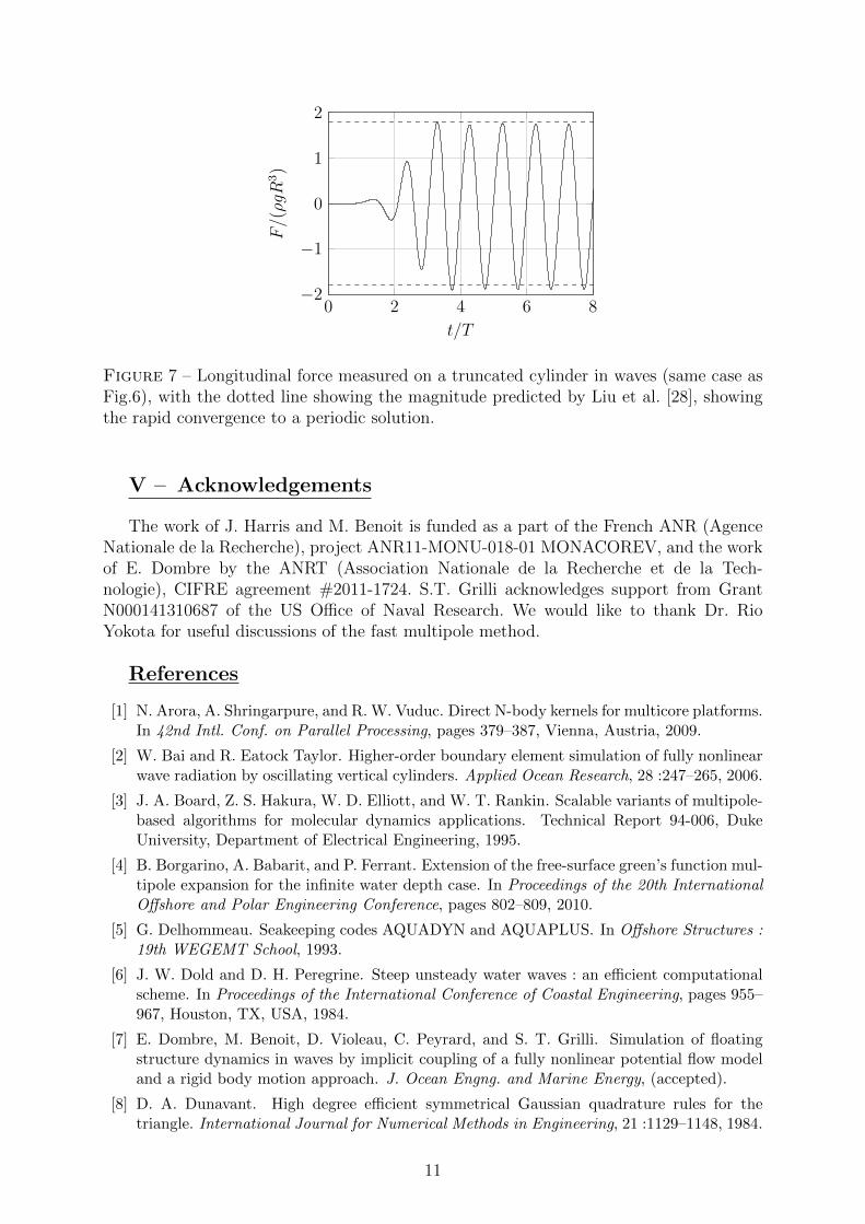
We consider a grid of N = 8591 collocation nodes (17194 elements), with 18 pointsaround the waterline of the cylinder, and simulate 8 wave periods. The first-order forcecoefficient is easily computed (Fig. 7), which we see gives results identical to Liu et al. andis within the range of other results listed in Table 1. The agreement with the second-orderforce is less good, but there is considerable variation in earlier published results .

IV – Summary

We showed results of a new implementation of a FMM-accelerated BEM-NWT forwave-structure interactions, giving solution times competitive with existing methods. Thisapproach solves in the time-domain for fully nonlinear potential flow, on unstructured 3Dgrids with linear triangular elements. If we compare the performance of this NWT withthat of Grilli et al. [14], as expected, we see that the earlier NWT, which is higher-order,achieves better conservation of energy and volume, but it does not scale well in CPUtime/numerical complexity, beyond a few thousand DOFs. By contrast the present NWThas the potential for achieving similarly accurate results with O(N) scaling.

Further modifications of the present unstructured grid code are necessary to use higher-order elements. Still, we clearly see that the FMM is very efficient for solving Laplace’sequation, and it is possible to use it with limited modification the established libraryExaFMM [39]. Additional results, with finer grid resolution, and demonstrating the pa-rallel performance of the complete NWT, will be shown at the conference.

10

0 2 4 6 8−2

−1

0

1

2

t/T

F/(ρgR

3)

Figure 7 – Longitudinal force measured on a truncated cylinder in waves (same case asFig.6), with the dotted line showing the magnitude predicted by Liu et al. [28], showingthe rapid convergence to a periodic solution.

V – Acknowledgements

The work of J. Harris and M. Benoit is funded as a part of the French ANR (AgenceNationale de la Recherche), project ANR11-MONU-018-01 MONACOREV, and the workof E. Dombre by the ANRT (Association Nationale de la Recherche et de la Tech-nologie), CIFRE agreement #2011-1724. S.T. Grilli acknowledges support from GrantN000141310687 of the US Office of Naval Research. We would like to thank Dr. RioYokota for useful discussions of the fast multipole method.

References

[1] N. Arora, A. Shringarpure, and R. W. Vuduc. Direct N-body kernels for multicore platforms.In 42nd Intl. Conf. on Parallel Processing, pages 379–387, Vienna, Austria, 2009.

[2] W. Bai and R. Eatock Taylor. Higher-order boundary element simulation of fully nonlinearwave radiation by oscillating vertical cylinders. Applied Ocean Research, 28 :247–265, 2006.

[3] J. A. Board, Z. S. Hakura, W. D. Elliott, and W. T. Rankin. Scalable variants of multipole-based algorithms for molecular dynamics applications. Technical Report 94-006, DukeUniversity, Department of Electrical Engineering, 1995.

[4] B. Borgarino, A. Babarit, and P. Ferrant. Extension of the free-surface green’s function mul-tipole expansion for the infinite water depth case. In Proceedings of the 20th InternationalOffshore and Polar Engineering Conference, pages 802–809, 2010.

[5] G. Delhommeau. Seakeeping codes AQUADYN and AQUAPLUS. In Offshore Structures :19th WEGEMT School, 1993.

[6] J. W. Dold and D. H. Peregrine. Steep unsteady water waves : an efficient computationalscheme. In Proceedings of the International Conference of Coastal Engineering, pages 955–967, Houston, TX, USA, 1984.

[7] E. Dombre, M. Benoit, D. Violeau, C. Peyrard, and S. T. Grilli. Simulation of floatingstructure dynamics in waves by implicit coupling of a fully nonlinear potential flow modeland a rigid body motion approach. J. Ocean Engng. and Marine Energy, (accepted).

[8] D. A. Dunavant. High degree efficient symmetrical Gaussian quadrature rules for thetriangle. International Journal for Numerical Methods in Engineering, 21 :1129–1148, 1984.

11

[9] O. M. Faltinsen, J. N. Newman, and T. Vinje. Nonlinear wave loads on a slender verticalcylinder. Journal of Fluid Dynamics, 289 :179–198, 1995.

[10] C. Fochesato and F. Dias. A fast method for nonlinear three-dimensional free-surface waves.Proceedings of the Royal Society A, 462 :2715–2735, 2006.

[11] C. Fochesato, S. T. Grilli, and F. Dias. Numerical modeling of extreme rogue waves gene-rated by directional energy focusing. Wave Motion, 44 :395–416, 2007.

[12] C. Fochesato, S. T. Grilli, and P. Guyenne. Note on non-orthogonality of local curvilinearco-ordinates in a three-dimensional boundary element method. International Journal forNumerical Methods in Fluids, 48 :305–324, 2005.

[13] L. Greengard and V. Rokhlin. A fast algorithm for particle simulations. Journal of Com-putational Physics, 73 :325–348, 1987.

[14] S. T. Grilli, P. Guyenne, and F. Dias. A fully nonlinear model for three-dimensional overtur-ning waves over arbitrary bottom. International Journal for Numerical Methods in Fluids,35 :829–867, 2001.

[15] S. T. Grilli and J. Horrillo. Generation and absorption of fully nonlinear periodic waves.Journal of Engineering Mechanics, 123 :1060–1069, 1997.

[16] S. T. Grilli, J. Skourup, and I. A. Svendsen. An efficient boundary element method fornonlinear water waves. Engineering Analysis with Boundary Elements, 6 :97–107, 1989.

[17] S. T. Grilli and R. Subramanya. Numerical modeling of wave breaking induced by fixed ormoving boundaries. computational mechanics. Computat. Mech., 17(6) :374–391, 1996.

[18] S. T. Grilli, S. Vogelmann, and P. Watts. Development of a 3d numerical wave tank for mo-deling tsunami generation by underwater landslides. Engineering Analysis with BoundaryElements, 26(4) :301–313, 2002.

[19] E. Guerber, M. Benoit, S. T. Grilli, and C. Buvat. A fully nonlinear implicit model forwave interactions with submerged structures in forced of free motion. Engineering Analysiswith Boundary Elements, 36 :1151–1163, 2012.

[20] P. Guyenne and S. T. Grilli. Numerical study of three-dimensional overturning waves inshallow water. Journal of Fluid Mechanics, 547 :361–388, 2006.

[21] J. C. Harris, E. Dombre, M. Benoit, and S. T. Grilli. Fast integral equation methods forfully nonlinear water wave modeling. In Proceedings of the 24th International Offshore andPolar Engineering Conference, pages 583–590, Busan, Korea, 2014.

[22] T. Ishiyama, K. Nitadori, and J. Makino. 4.45 Pflops astrophysical N-body simulation onK computer - the gravitational trillion-body problem. In Proceedings of the InternationalConference on High Performance Computing, Networking, Storage and Analysis, page 10pp., Salt Lake City, UT, USA, 2012.

[23] H. M. Kim and D. K. P. Yue. The complete second-order diffraction solution for an axisym-metric body. Part I. Monochromatic incident waves. Journal of Fluid Dynamics, 200 :235–264, 1989.

[24] D. C. Kring, F. T. Korsmeyer, J. Singer, D. Danmeier, and J. White. Accelerated nonlinearwave simulations for large structures. In 7th International Conference on Numerical ShipHydrodynamics, Nantes, France, 1999.

[25] J. R. Krokstad and C. T. Stansberg. Ringing load models verified against experiments. InProceedings of the International Conference on Offshore Mechanics and Arctic Engineering,Copenhagen, Denmark, 1995.

[26] C. H. Lee. WAMIT Theory Manual. Technical report, MIT, 1995. Report 95-2, Departmentof Ocean Engineering.

12

[27] L. Letournel, J. C. Harris, P. Ferrant, A. Babarit, G. Ducrozet, E. Dombre, and M. Be-noit. Comparison of fully nonlinear and weakly nonlinear potential flow solvers for thestudy of wave energy converters undergoing large amplitude motions. In Proceedings of the33rd International Conference on Ocean, Offshore and Arctic Engineering, page 23912, SanFrancisco, USA, 2014.

[28] Y. Liu, M. Xue, and D. K. P. Yue. Computations of fully nonlinear three-dimensional wave-wave and wave-body interactions. Part 2. Nonlinear waves and forces on a body. Journalof Fluid Dynamics, 438 :41–66, 2001.

[29] Y. H. Liu, C. H. Kim, and X. S. Kim. Comparison of higher-order boundary element andconstant panel methods for hydrodynamic loadings. International Journal of Offshore andPolar Engineering, 1 :8–17, 1991.

[30] M. S. Longuet-Higgins and E. Cokelet. The deformation of steep surface waves on water, I.A numerical method of computation. Proceedings of the Royal Society A, 350 :1–26, 1976.

[31] S. B. Nimmala, S. C. Yim, and S. T. Grilli. An efficient parallelized 3-D FNPF numericalwave tank for large-scale wave basin experiment simulation. Journal of Offshore Mechanicsand Arctic Engineering, 135 :021104, 2013.

[32] W. T. Rankin. Efficient parallel implementations of multipole based N-body algorithms.PhD thesis, Duke University, Department of Electrical Engineering, 1999.

[33] Y.-L. Shao and O. M. Faltinsen. A harmonic polynomial cell (HPC) method for 3D Laplaceequation with application in marine hydrodynamics. Journal of Computational Physics,274 :312–332, 2014.

[34] H. G. Sung and S. T. Grilli. A note on accuracy and convergence of a third-order boundaryelement method for three dimensional nonlinear free surface flows. Journal of Ships andOcean Engineering, 40 :31–41, 2005.

[35] H. G. Sung and S. T. Grilli. Numerical modeling of nonlinear surface waves caused bysurface effect ships dynamics and kinematics. In Proceedings of the 15th InternationalOffshore and Polar Engineering Conference, 2005.

[36] H. G. Sung and S. T. Grilli. Bem computations of 3d fully nonlinear free surface flowscaused by advancing surface disturbances. International Journal of Offshore and PolarEngineering, 18(4) :292–301, 2008.

[37] K. Tanizawa. The state of the art on numerical wave tank. In Proceedings of 4th OsakaColloquium on Seakeeping Performance of Ships, pages 95–114, 2000.

[38] R. Yokota. An FMM based on dual tree traversal for many-core architectures. Journal ofAlgorithms and Computational Technology, 7 :301–324, 2013.

[39] R. Yokota, J. P. Bardhan, M. G. Knepley, L. A. Barba, and T. Hamada. Biomolecularelectrostatics using a fast multipole BEM on up to 512 GPUs and a billion unknowns.Computer Physics Communications, 182 :1272–1283, 2011.

13