Positive Solutions of Nonlinear Elliptic Boundary Value ... · JOURNAL OF MATHEMATICAL ANALYSIS AND...

JOURNAL OF MATHEMATICAL ANALYSIS AND APPLICATIONS 51, 461-482 (1975)

Positive Solutions of Nonlinear Elliptic

Boundary Value Problems

ROGER NUSSBAUM*

Rutgers U~tiversity, New Brunswick, New Jersey 08903

Submitted by Peter D. Lax

This paper considers the problem of finding positive vector-valued solutions U of the nonlinear elliptic boundary value problem L(U) + f(x, U) = 0 on a bounded region Q, U + aU/av = 0 on a9. The operator L is uniformly elliptic and in divergence form, and f is, roughly speaking, superlinear; by the positivity of U is meant the positivity of each component of U on Q. Under certain growth conditions on f and some further technical assumptions, the existence of a positive solution is proved, an a priori bound on all positive solutions is obtained, and a certain fixed point index is proved equal to - 1. As an example, information about fixed point indices is used to allow perturbations of the form eh(x, U, DU). In the final section, an essentially best possible theorem is given for Q a ball and for radially symmetric solutions of the Laplacian with Dirichlet boundary conditions.

We shall be interested in this paper in finding “positive” vector valued solutions U of the second-order nonlinear elliptic boundary problem L(U) + f(~, U) = 0 on 52, U + y(aU/&) = 0 on 3.Q. By “positive” we shall mean that all components of U are positive on L?. The operator L will be

uniformly elliptic and in divergence form and the nonlinear term will, roughly speaking, be of superlinear type.

The structure of this paper is as follows. In the first section, we recall necessary information about the fixed point index and fixed point theorems for self-mappings of a cone. The second section applies this material to the study of the nonlinear boundary value problems. The main theorem (Theo- rem 2.1) establishes the existence of positive solutions and, perhaps more importantly, gives an a priori bound on all positive solutions and shows that certain fixed point indices are Al. The drawback of Theorem 2.1 is that it demands that ) f(~, U)l < B + 1 U 10, where CJ must be less than n/(n - 1) if the function y above is identically zero on X?, (r must be less than ~/(Pz - 2

* Partially supported by NSF GP 20228 and a Rutgers Research Council Faculty Fellowship.

461 Copyright 0 1975 by Academic Press, Inc. All rights of reproduction in any form reserved.

462 ROGER NUSSBAUM

if y is strictly positive on &‘, and n is the dimension of the space. There is

reason to suspect that the proper bound on (T is (n + 2)/(n - 2). The third section of this paper gives a simple extension of Theorem 2.1 which indicates

the usefulness of proving certain fixed point indices are &l. Though we do not make extensive use of information about fixed point indices here, we hope to show in a future paper how this can be used to study bifurcation and establish the existence of unbounded continua of solutions for the eigenvalue problem L(U) + Xf(x, U) = 0 on Q, U + r(aU/&) = 0 on 8Q. The final section considers the very special case L = the Laplacian, Q = a ball, and U = real-valued function and shows how a priori

bounds can be obtained on all positive radially symmetric solutions for CT < (n + 2)/(n - 2).

The question of positive solutions of nonlinear elliptic boundary value problems is the subject of a large literature; references [l] and [2] give some further guides to the literature. The recent article [2] by Ambrosetti and Rabinowitz is probably closest in its results (though not its methods) to our results here. Ambrosetti and Rabinowitz study the question of finding

positive real-valued solutions u of the boundary value problem

Lu +f@, u) = 0, u = 0 on &Q.

By putting certain technical conditions on f and assuming that

If@, 41 < B + c I u lo n+2 foro<n--2,

they prove by variational methods the sharp result that the boundary value

problem has a positive solution. However, they do not obtain a priori bounds in this case and they do not obtain information about a fixed point index.

We should mention that although [l] h as a surface similarity to our work (in the use of theorems about the fixed point index and expansions of a cone), the basic techniques are quite different. Our basic problem is to find a priori bounds and the methods in [l] avoid the problems of a priori bounds and do not in general apply to the equations we consider.

1. In this section we recall a few known theorems and definitions. If A

is a bounded subset of a Banach space X, then we follow C. Kuratowski [9] and define r(A), the measure of noncompactness, to be inf{d > 0: A is a finite union of sets of diameter less than d}. There are other possible definitions of a measure of noncompactness, and one can speak of a generalized measure of noncompactness in the sense of [14, Sect. 11. If D is a subset of a Banach space X and f: D - X is a continuous map which takes bounded sets to bounded sets, we shall say that f is a condensing map if for every set A C D such that y(A) > 0 we have y[ f (A)] < y(A).

NONLINEAR ELLIPTIC BOUNDARY VALUE PROBLEMS 463

I f D is a closed convex subset of a Banach space X, G is a bounded and open subset of D (open in the relative topology on D) and f: G+ D is a condensing map such that f(x) # x for x E G - G, then there is defined an integer ;n(f, G) called the fixed point index off on G. A full development of this fixed point index is given (in much greater generality) in [12], and the various properties of the fixed point index are developed there. Summaries of these results can be found in [l 11. Since we shall not be using the fixed point

index extensively here, we only recall the basic result that if ;n(f, G) # 0, f has a fixed point in G.

If D is a closed convex subset of a Banach space X, we shall say that D is a “wedge” if whenever x E D, then tx E D for t > 0. The following theorem,

which is a special case of Lemma 1.3 in [13], is the only fixed point theorem we shall need. It can be viewed as a generalization of Krasnoselskii’s theorems in [6, 71 concerning expansions of a cone. Different generalizations have been given by J. D. Hamilton in [5] and G. M. Goncharov in [4].

THEOREM 1.1. (See Lemma 1.3 in [13].) Assume that K is a wedge in a Banach space X and that r and R are positive numbers with r < R. Define

G = {x E K: jj x 11 < R} and assume that @: c--+ K is a condensing map. Assume that there exists v E K with v # 0 such that x - a(x) # tv for all

x E K with /I x 1) = R and all t > 0. Finally suppose that x - t@(x) # 0 for all x E K with I/ x 11 = r and for 0 < t < 1. Then if

lJ=(x~K:r <llxll <R},

it follows that iK(@, U) = - 1 and @ has a $xed point in U. If

0 = {x 6 K: I/ x I/ < r},

it is also true that iK(@, 0) = 1 and iK(@, G) = 0.

2. I f G is a smooth bounded domain in Rn and u: s + R is a C2 real- valued function on a, then for Cr real-valued coefficients aij(x) we can consider the operator Lu = z:i,j (r~~~u,~),~ . Similarly, if U: 0 + RN is a C2 vector-valued function, we can also consider L(U) = Ci,j (u,~U,.J,. . Denote the set {U E RN: U = (ur , ua ,..., uN) and ui > 0 for 1 < i < IV) by Q and let f:o x Q-Q b e a Holder continuous function such that f (x, 0) = 0 for x E Sz. We are interested here in the following closely related questions: Under what conditions on L and f will there exist a positive vector function U: G-Q such that (LU) (x) + f [x, U(x)] = 0 for x E Sz and U + y(aU/&) = 0 on &’ and will there exist an a priori bound on all such positive solutions ?

409/51/2-I4

464 ROGER NUSSBAUM

To make our problem more precise, we make the following regularity assumptions on Sz, L, and f.

ASSUMPTION Rl. There exists a positive constant a > 0 such that for each x E asZ, there exists a ball B of radius a such that x E aB and B CD. The boundary afi of Q is of class C (2J)(0 < h < 1); and if q(x) denotes the outward normal vector to Sz at x E X?, the map x--f T(X) is of class CIJ).

ASSUMPTION R2. The real-valued functions a,$: Q-+ R are elements of C(l+V$) for 1 < ;,j < n (that is, the derivatives of adj exist and are Holder continuous with Holder constant A) and qi(x) = uji(x) for 1 < ;, j 6 n. The operator L is uniformly elliptic, so that there exists a positive constant c such that Ci,j uii(x) ti& > c 1 5 I2 for all x EJ=? and f E Rn. Finally, the function y: asZ + R is a C 1-A function which is either positive on aL? or identically zero; we shall denote by y(aU/&) the conormal derivative with respect to L: y(aujav) = yxi,j u~~QU,.+ where q(x) is the outward normal at x.

In order to state our conditions on f we need some further definitions and notations. Suppose that a: 0 -P R is an element of CA@) (0 < X < 1) and that u(x) > 0 for x ~a. Consider the eigenvalue problem

and (Lv) (-4 + w(x) v(x) = 0 for x E D

V(X) + Y(X) (av/av) = 0 for x E af2.

It is known that this problem has a smallest eigenvalue p = A, > 0 and has a corresponding eigenvector z, such that 21 is positive on 0 if y(x) > 0 for x E ZJ or V(X) > 0 for x E 52 and (a+) < 0 on asZ if Y(X) z 0 for x E Z?. These results can be obtained from the Krein-Rutman theorem in [8]; more detailed proofs are given in [16, pp. 5055061 and in [l]. We shall consistently use A, to refer to this smallest eigenvalue and v to refer to a fixed positive eigenvector corresponding to A, .

In the following conditions on f, we use fi to denote the ith component of the map f:o+Q+RN and for u=(ul,...,uN) we define

ASSUMPTION R3. The vector-valued function f: D x Q--f Q is Holder continuous with Holder constant h > 0. There exists a constant p > A1 = the smallest eigenvalue and a constant R such that fi(x, U) > @z(x) ui if Ui > R.

SONLINEAR ELLIPTIC BOUNDARY VALUE PROBLEMS 465

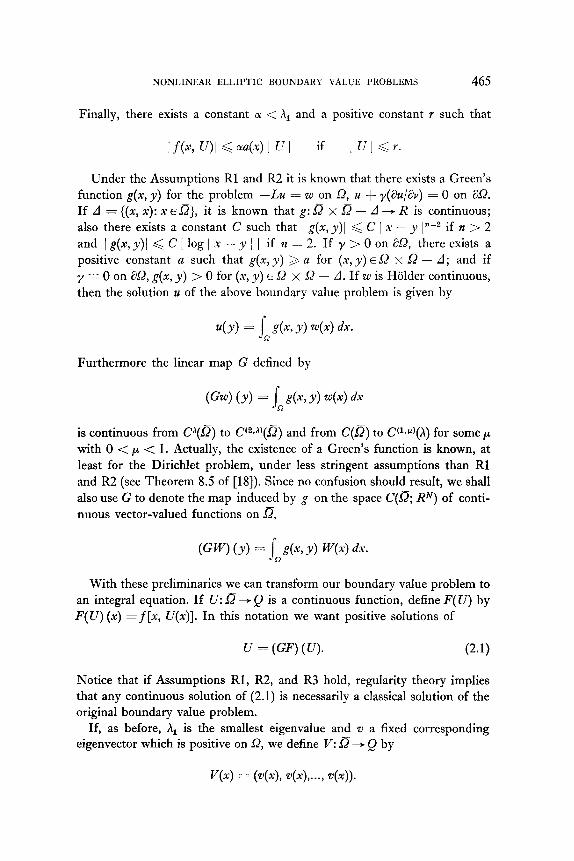
Finally, there exists a constant 01 < X, and a positive constant r such that

Under the Assumptions RI and R2 it is known that there exists a Green’s function g(x, y) for the problem -Lu = w on L?, u + y(&/&) = 0 on LX’. I f d = {(x, x): x EO}, it is known that g: fi x fi - d -+ R is continuous; also there exists a constant C such that j g(x, y)i < C 1 x - y ln-2 if n > 2

and l&,y)l <Cllog/ x - y j 1 if n = 2. If y > 0 on 8Q, there exists a positive constant a such that g(x, y) > a for (x, y) EQ x s - d; and if y = 0 on a52, g(x, y) > 0 for (x, y) E 9 x L? - d. I f w is Holder continuous, then the solution u of the above boundary value problem is given by

U(Y) = ja .&Ax, Y> 44 dx*

Furthermore the linear map G defined by

(Gw) (Y) = j, &P Y) w(x) dx

is continuous from C”(D) to Ce+$) and from C(o) to C1*u)(A) for some ,U with 0 < p < 1. Actually, the existence of a Green’s function is known, at

least for the Dirichlet problem, under less stringent assumptions than RI and R2 (see Theorem 8.5 of [18]). S’ mce no confusion should result, we shall also use G to denote the map induced by g on the space C@; RN) of continuous vector-valued functions on s,

(GV (Y) = jn Ax, y) W(x) dx.

With these preliminaries we can transform our boundary value problem to an integral equation. If U: Q---f Q is a continuous function, define F(U) by F(U) (x) =f[x, U(x)]. In th is notation we want positive solutions of

U = (GF) (U). (2.1)

Notice that if Assumptions RI, R2, and R3 hold, regularity theory implies that any continuous solution of (2.1) is necessarily a classical solution of the original boundary value problem.

If, as before, Xi is the smallest eigenvalue and zi a fixed corresponding eigenvector which is positive on !S, we define V: D + Q by

466 ROGER NUSSBAUM

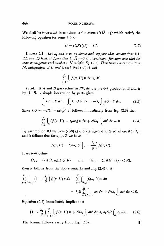
We shall be interested in continuous functions U: 0 -+ Q which satisfy the following equation for some t > 0:

U = (GF)(U) + tV. 0.2)

LEMMA 2.1. Let h, and v be as above and suppose that assumptions Rl, R2, and R3 hold. Suppose that U: Q + Q is a continuous function such that for

some nonnegative real number t, U satisfies Eq. (2.2). Then there exists a constant M, independent of U and t, such that t < M and

Proof. If A and B are vectors in RN, denote the dot product of A and B

by A * B. A simple integration by parts gives

s LU.Vdx= aU. Vdx.

52 s U.LVdx = --h, (2.3)

sa s D

Since LU = -FU - tah,V, it follows immediately from Eq. (2.3) that

$ In (f&, U) - ha%) ZJ dx + Nth, J ,̂ av2 dx = 0. (2.4)

By assumption R3 we have (X,//3) fi(x, U) > h,aui if ui 2 R, where /3 > h, , and it follows that for ui >, R we have

fi(x, U) - /\,aui 3 [ 1 - +] fi(x, U).

If we now define

J-2,,, = {x E Q: ui(x) > R} and .L& = {x E Q: ui(x) < R},

then it follows from the above remarks and Eq. (2.4) that

gl s,, i (1 - +) fib U> v dx + ?I Jn, ifi(x, U) w dx ’

- X,R $ 1 av dx + Nth, 1 av2 dx < 0. i=l Q2.i a

Equation (2.5) immediately implies that

(1 - +) zl j+,fib U> u + Nth, s av2 dx < h,NR s

av dx. (2.6) a Q

The lemma follows easily from Eq. (2.6). I

NONLINEAR ELLIPTIC! BOUNDARY VALUE PROBLEMS 467

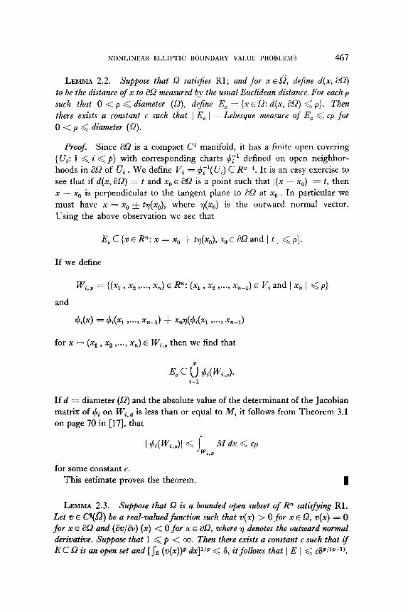
LEMMA 2.2. Suppose that Q satisJies Rl; and for x ~0, dejine d(x, aQ> to be the distance of x to aQ measured by the usual Euclidean distance. For each p

such that 0 .

Proof. Since &‘2 is a compact Cl manifold, it has a finite open covering (Vi: 1 < i < p} with corresponding charts 4;’ defined on open neighbor- hoods in aQ of oi . We define Vi = +;‘( Ui) C Rn-l. It is an easy exercise to see that if d(x, LX2) = t and x0 E Z&2 is a point such that I(x - x,)1 = t, then x - xs is perpendicular to the tangent plane to X2 at x0 . In particular we

must have x = x0 & ty(x,J, where 7(x,,) is the outward normal vector. Using the above observation we see that

E, C {x E R”: x = x,, f tv(x,J, x0 E X2 and j t 1 < p}.

I f we define

W,,, = {(x1 , x2 ,..., x,) E Rn: (x1 , x2 ,..., x,-r) E Vi and I X, I 

and

h(x) = A(% ,-..3 X,-l) + WMXl Y...P xn-1)

for x = (x1 , x2 ,..., x,) E W,,, then we find that

If d = diameter (a) and the absolute value of the determinant of the Jacobian matrix of #i on Wi,& is less than or equal to M, it follows from Theorem 3.1 on page 70 in [ 171, that

for some constant c. This estimate proves the theorem. a

LEMMA 2.3. Suppose that Q is a bounded open subset of R” satisfying RI. Let v E Cl(a) be a real-valued function such that v(x) > 0 for x E 52, v(x) = 0 for x E 352 and (8v/&) (x) < 0 for x E al& where 7 denotes the outward normal derivative. Suppose that 1 < p < co. Then there exists a constant c such that if E C Q is an open set and [ fE (v(x))” d x l/p < 8, it follows that 1 E 1 < c@/(*+~). ]

468 ROGER NUSSBAUM

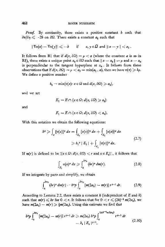
Proof. By continuity, there exists a positive constant b such that &/a~ < -26 on 8.0. There exists a constant a, such that

[I VW(X) - Vv(y)ll < -b if X,YE~ and lx----yII <a,.

It follows from Rl that if d(x, 3.Q) = p < a (where the constant u is as in Rl), there exists a unique point x,, E asZ such that II x - x0 11 = p and x - x0 is perpendicular to the tangent hyperplane at x,, . It follows from these observations that if d(x, aQ> = p < a2 = min(a, , a), then we have v(x) 3 bp. We define a positive number

b, = min{u(x): x E 52 and d(x, a52) > a,},

and we set

and

El = E n {x E L’: d(x, aQ) < uZ}.

With this notation we obtain the following equations:

8” 2 j- MO’ dx = s, b(x)]” dx + f, [+)I” dx E

3 blP I -‘A I + jEI P(xP dx. (2.7)

If m(r) is defined to be 1(x E Q: d(x, X?) < r and x E El}/ , it follows that

JEl w(x)” dx >, Ioza’ (br)p dm(r).

If we integrate by parts and simplify, we obtain

(2.8)

Ia2 (br)p dm(r) = by ha” [m(2u,) - m(r)] rp-l dr. (2.9)

According to Lemma 2.2, there exists a constant k (independent of E and 6) such that M(Y) < kr for 0 < Y. It follows that for 0 < r < (2k)-1m(2u,), we have m(24 - m(r) 3 +42u,). Using this estimate we find that

by I”’ [m(2a2) - m(r)] @-I dr > m(2u,) bpp s W-'m(2a*)

r P--l dr

= k, 1 El jp+l, ’ (2.10)


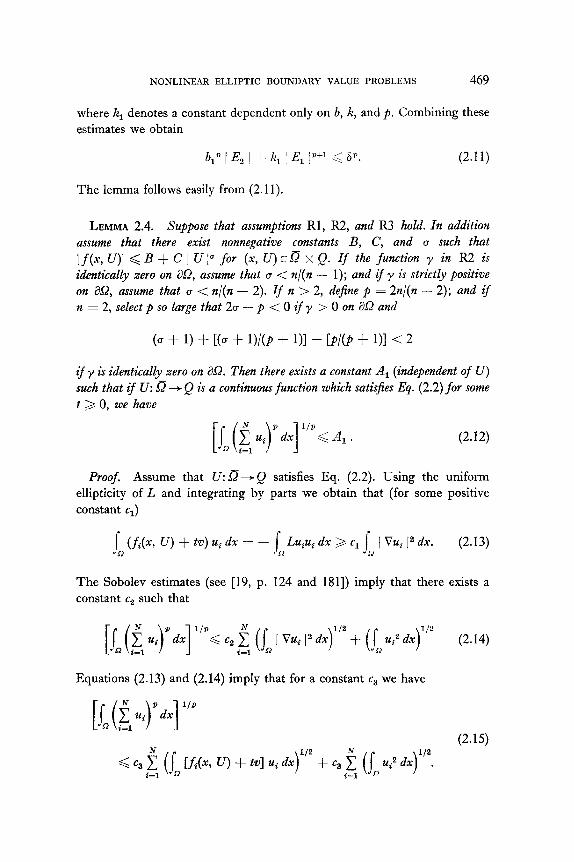
where k, denotes a constant dependent only on b, k, and p. Combining these estimates we obtain

blp 1 E, / + k, 1 El jp+l <: Sn. (2.11)

The lemma follows easily from (2.11).

LEMMA 2.4. Suppose that assumptions Rl, R2, and R3 hold. In addition assume that there exist nonnegative constants B, C, and u such that If(x, U)j 2, de&e p = 2n/(n - 2); and if n = 2, select p so large that 2a - p < 0 if y > 0 on aQ and

(u + 1) + [(u + l)l(P + 111 - [P/(P + 111 < 2

ifr is identically zero on %I. Then there exists a constant A, (independent of U)

such that if V:s+Q is a continuous function which satisfies Eq. (2.2) for some

t 3 0, we have

(2.12)

Proof. Assume that U: &+ Q satisfies Eq. (2.2). Using the uniform ellipticity of L and integrating by parts we obtain that (for some positive constant cI)

j-, (f&q U) + tv) ui dx = - jDLu,ui dx 3 cl .c, 1 Vu, I2 dx. (2.13)

The Sobolev estimates (see [ 19, p. 124 and 1811) imply that there exists a constant c, such that

gl cs, I Vui 1’ dx)1’2 + (s, ui2 dx)1’2 (2.14)

Equations (2.13) and (2.14) imply that for a constant cs we have

(2.15)

< ~3 f (J [fi(X, U) + tV] Ui dx)li2 + ~2 2 (1 ui2 dx)“‘. ix1 I2 &l 0

470 ROGER NUSSBAUM

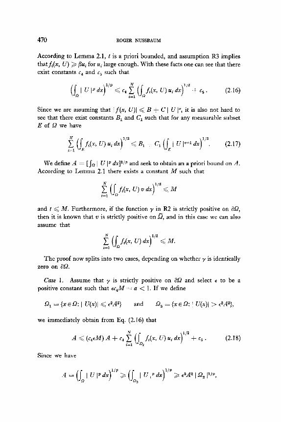
According to Lemma 2.1, t is a priori bounded, and assumption R3 implies thatfi(x, U) 3 flui for ui large enough. With these facts one can see that there exist constants cq and c5 such that

(2.16)

Since we are assuming that / f(~, U)[ < B + C 1 U IV, it is also not hard to see that there exist constants B, and C, such that for any measurable subset E of Sz we have

f (j fi(x, U) ui ~Jx)l’~ < B, + C, (s, j U [~+l d~)l’~. (2.17) i=l E

We define A = [SD / U ID ~x]~/P and seek to obtain an a priori bound on A. According to Lemma 2.1 there exists a constant M such that

f (j f&r, U) v dx)li2 < M i-1 .Q

and t < M. Furthermore, if the function y in R2 is strictly positive on aQ, then it is known that D is strictly positive on a, and in this case we can also assume that

f (j fi(x, U) d~)~‘~ < M. i-1 n

The proof now splits into two cases, depending on whether y is identically zero on aQ.

Case 1. Assume that y is strictly positive on &Q and select E to be a positive constant such that cc4M = a < 1. If we define

Sz, = {x E 52: I U(x)/ < c2A2} and Q2 = (x EL?: j U(x)1 > c2A2},

we immediately obtain from Eq. (2.16) that

Since we have

c&f) A + c4 f (j fi(x, U) ui d~)l'~ i i=l %

c5 . (2.18)


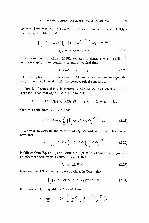
we must have that 1 52, 1 < (GA)-n. If we apply this estimate and Holder’s inequality, we obtain that

< c-2P+20+2iqotl-P+o+1~ (2.19)

If we combine Eqs. (2.17), (2.18), and (2.19), define T = u - (p/2) + 1, and select appropriate constants c, and c7 we find that

A < aA + c6AT + c, . (2.20)

The assumption on u implies that Q- < 1, and since we also arranged that a < 1, we must have A ,( A, , for some a priori constant A, .

Case 2. Assume that y is identically zero on SJ and select a positive constant E such that EC*M = a < 1. If we define

52, = (x E Q: / U(x)1 < E2A%(X)2} and Q, = Q - Ql ,

then we obtain from Eq. (2.16) that

(2.21)

We wish to estimate the measure of Q, . According to our definition we have that

A = ( jQ 1 U IP dx)l” > c2A2 (j,, vz’ dx)? 2

(2.22)

It follows from Eq. (2.22) and Lemma 2.3 (since it is known that av/$ < 0 on &Q) that there exists a constant cs such that

1 Q, 1 < C&m+l)l.

I f we use the Holder inequality we obtain as in Case 1 that

s / TJ lo+1 dx < Au+1 1 Q, Il-Ko+l)l~l.

%

(2.23)

(2.24)

If we now apply inequality (2.23) and define

472 ROGER NUSSBAUM

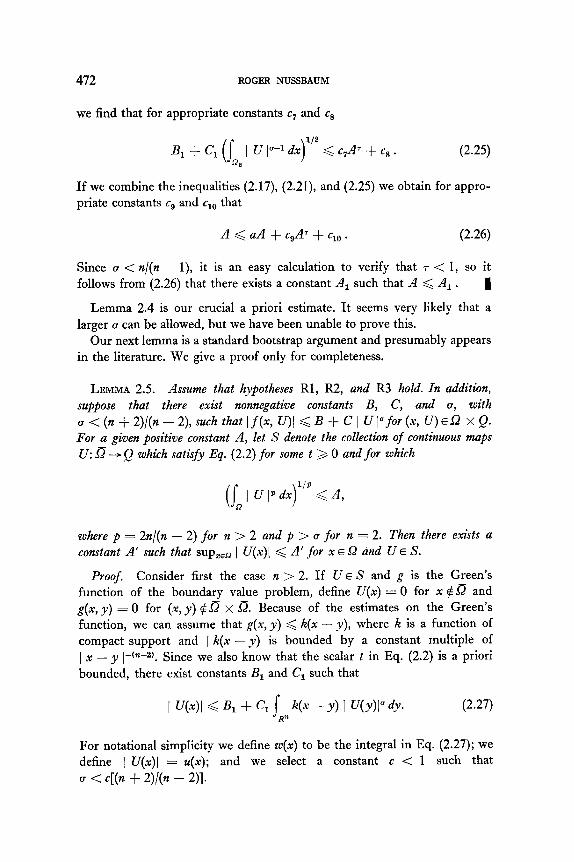
we find that for appropriate constants c, and cs

B, + Cl (j-,2 1 U Iof dx)“’ < c,A’ + cs . (2.25)

If we combine the inequalities (2.17) (2.21), and (2.25) we obtain for appropriate constants cg and cl0 that

A < aA + c,AT + cl0 . (2.26)

Since u < n/(n - l), it is an easy calculation to verify that T < 1, so it follows from (2.26) that there exists a constant A, such that A < A, . 1

Lemma 2.4 is our crucial a priori estimate. It seems very likely that a larger a can be allowed, but we have been unable to prove this.

Our next lemma is a standard bootstrap argument and presumably appears in the literature. We give a proof only for completeness.

LEMMA 2.5. Assume that hypotheses RI, R2, and R3 hold. In addition, suppose that there exist nonnegative constants B, C, and u, with

0 < (n + 2)l(n - 9, such that 1 f(x, U)i 0 and for which

where p = 2n/(n - 2) for n > 2 and p > (T for n = 2. Then there exists a constant A’ such that SUP,.~ I U(x)1 < A’ for x E Sz and U E S.

Proof. Consider first the case n > 2. If U E S and g is the Green’s function of the boundary value problem, define U(x) = 0 for x #Q and g(x, y) = 0 for (x, y) $Q x Q. Because of the estimates on the Green’s function, we can assume that g(x, y) < K(x - y), where K is a function of compact support and I k(x - y) is bounded by a constant multiple of ( x - y I-(n-2). Since we also know that the scalar t in Eq. (2.2) is a priori bounded, there exist constants B, and C, such that

I W9l G 4 + G 1 4~ - Y) I Us” 4v (2.27) Rn

For notational simplicity we define w(x) to be the integral in Eq. (2.27); we define 1 U(x)\ = u(x); and we select a constant c < 1 such that 0 < cl+ + 2>/(n - 31.


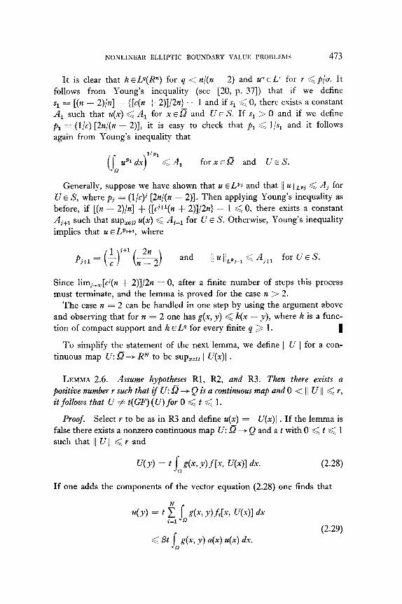
It is clear that k ELQ(Rn) for q < n/(n - 2) and u” E L’ for r <p/u. It follows from Young’s inequality (see [20, p. 371) that if we define

s, = [(n - q/4 + {[c(n + 2)1/W - 1 and if sr :< 0, there exists a constant A, such that U(X) < A, for x EQ and U E S. If sr > 0 and if we define

p, = (l/c) [2n/(n - 2)], it is easy to check that p, < l/s, and it follows again from Young’s inequality that

(s, ~2’1 dx)- < A, forx&D and UES.

Generally, suppose we have shown that u ELP~ and that I] u ilLDj < A? for

U E S, where pj = (l/c)j [2n/(n - 2)]. Th en applying Young’s inequality as

before, if [(n - 2)/n] + {[ci+l(n + 2)]/2n) - 1 < 0, there exists a constant Aj+l such that sup,,o U(X) < Aj+l for U E 5’. Otherwise, Young’s inequality

implies that u E LPj+l, where

Since limj,m[cj(n + 2)]/2n = 0, after a finite number of steps this process must terminate, and the lemma is proved for the case n > 2.

The case PZ = 2 can be handled in one step by using the argument above and observing that for n = 2 one has g(x, y) < tZ(x - y), where k is a func-

tion of compact support and Iz +z Lq for every finite q > 1. I

To simplify the statement of the next lemma, we define jl U/I for a continuous map U: s-+ RN to be supren j U(X)] .

LEMMA 2.6. Assume hypotheses Rl, R2, and R3. Then there exists a

positive number r such that if U: 0 + Q is a continuous map and 0 < II U II < r, it follows that U # t(GF) (U) for 0 < t < 1.

Proof. Select r to be as in R3 and define U(X) = / U(X)] . I f the lemma is false there exists a nonzero continuous map U: Q + Q and a t with 0 < t < 1 such that ]I U11 < r and

U(Y) = t s, g(x, Y) fb 441 dx. (2.28)

If one adds the components of the vector equation (2.28) one finds that

I (2.29)

< Bt g(x) Y) 44 44 dx. R

474 ROGER NUSSBAUM

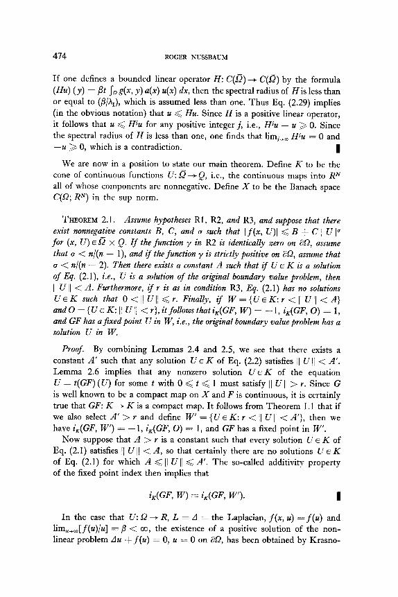
I f one defines a bounded linear operator H: C(o) --+ C(a) by the formula

(Hu) (y) = fit lo g(x, y) U(X) u(x) dx, then the spectral radius of His less than or equal to @/A,), which is assumed less than one. Thus Eq. (2.29) implies

(in the obvious notation) that u < Hu. Since H is a positive linear operator, it follows that u < HJu for any positive integer j, i.e., Hiu - u 3 0. Since the spectral radius of H is less than one, one finds that lirn+= Hiu = 0 and

-u 3 0, which is a contradiction. I

We are now in a position to state our main theorem. Define K to be the cone of continuous functions U: B--f Q, i.e., the continuous maps into RN all of whose components are nonnegative. Define X to be the Banach space C(sZ; RN) in the sup norm.

THEOREM 2.1. Assume hypotheses RI, R2, and R3, and suppose that there

exist nonnegative constants B, C, and u such that j f(x, U)l < B + C / U 10 for (x, U) EQ x Q. If the function y in R2 is identically zero on afi, assume that u < n/(n - I), and if the function y is strictly positive on asZ, assume that o < n/(n - 2). Then there exists a constant A such that if U E K is a solution

of Eq. (2.1), i.e., U is a solution of the original boundary value problem, then 11 U 11 < A. Furthermore, ;f r is as in condition R3, Eq. (2.1) has no solutions

UEK such that O<IjUll<r. Finally, if W={UEK:r<llUI/<A} andO={UEK:jjUjI <r>,itfollozusthati,(GF,W)=-l,i,(GF,O)=l, and GF has a$xed point U in W, i.e., the original boundary value problem has a

solution U in W.

Proof. By combining Lemmas 2.4 and 2.5, we see that there exists a constant A’ such that any solution U E K of Eq. (2.2) satisfies /I U 11 < A’. Lemma 2.6 implies that any nonzero solution U E K of the equation U = t(GF) (U) for some t with 0 < t < 1 must satisfy II U I/ > r. Since G

is well known to be a compact map on X and F is continuous, it is certainly true that GF: K + K is a compact map. It follows from Theorem 1.1 that if we also select A’ > r and define IV’ = {U E K: r < /] U /I < A’}, then we have i,(GF, W’) = -1, i,(GF, 0) = 1, and GF has a fixed point in IV’.

Now suppose that A > r is a constant such that every solution U E K of Eq. (2.1) satisfies // U II < A, so that certainly there are no solutions U E K of Eq. (2.1) for which A < I] U 11 < A’. The so-called additivity property of the fixed point index then implies that

i,(GF, W) = i,(GF, W’). I

In the case that U: Q + R, L = A = the Laplacian, f (x, u) = f (u) and lim,,,[f (u)/u] = ,5 < co, the existence of a positive solution of the non-

linear problem Au + f (u) = 0, u = 0 on aQ, has been obtained by Krasno-

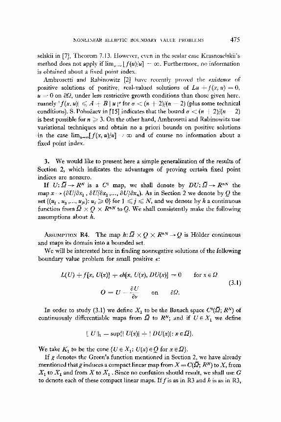
NONLINEAR ELLIPTIC BOUNDARY VALUE PROBLIXS 475

selskii in [7], Theorem 7.13. However, even in the scalar case Krasnoselskii’s method does not apply if lim,,+,[f(u)/u] = co. Furthermore, no information is obtained about a fixed point index.

Ambrosetti and Rabinowitz [2] have recently proved the existence of positive solutions of positive, real-valued solutions of Lu + f(x, u) = 0, u = 0 on asZ, under less restrictive growth conditions than those given here, namely /f(x, u)I < A + B ( u I0 for u < (n + 2)/(n - 2) (plus some technical conditions). S. Pohoiaev in [15] indicates that the bound 0 < (n + 2)/(n - 2) is best possible for n > 3. On the other hand, Ambrosetti and Rabinowitz use variational techniques and obtain no a priori bounds on positive solutions in the case limU+Jf(x, u)/u] = co and of course no information about a fixed point index.

3. We would like to present here a simple generalization of the results of Section 2, which indicates the advantages of proving certain fixed point indices are nonzero.

If U: a -+ RN is a Cl map, we shall denote by DU: B + RnN the map x-+(aU/ax, , au/ax, ,..., i3Ujax,). As in Section 2 we denote by Q the set i(ul , u2 ,..., UN): ui 3 0} for 1 <j < N, and we denote by h a continuous function from Q x Q x R nN to Q. We shall consistently make the following assumptions about h.

ASSUMPTION R4. The map h: a x Q x RnN - Q is Holder continuous and maps its domain into a bounded set.

We will be interested here in finding nonnegative solutions of the following boundary value problem for small positive E:

L(U) +f[x, U(x)] + 4x, U(x), DU(x)] = 0 for x E L?

0 = U+g on asz. (3-l)

In order to study (3.1) we define X, to be the Banach space Cl@; RN) of continuously differentiable maps from Q to RN; and if U E X, we define

II UII, = sup{/ U(x)1 + I DU(x)j: x ~0).

We take Kr to be the cone {U E Xl: U(x) E Q for x E !?}. If g denotes the Green’s function mentioned in Section 2, we have already

mentioned that g induces a compact linear map from X = C(a; RN) to X, from X1 to X1 and from X to X1 . Since no confusion should result, we shall use G to denote each of these compact linear maps. Iff is as in R3 and h is as in R3,

476 ROGER NUSSBAUM

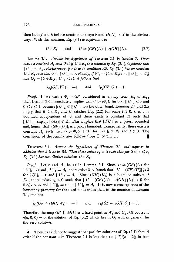
then both f and h induce continuous maps F and H: X, --f X in the obvious ways. With this notation, Eq. (3.1) is equivalent to

UEK, and U = (GF) (U) + E(GH) (U). (3.2)

LEMMA 3.1. Assume the hypotheses of Theorem 2.1 in Section 2. There exists a constant A, such that if U E KI is a solution of Eq. (2.1), it follows that 11 U II1 < A, . Furthermore, if r is as in condition R3, Eq. (2.1) has no solutions U E KI such that 0 < jj U/II < Y. FinaEZy, if WI = {U E K,: r < jj U II1 < A,} and 0, = (U E K,: 11 U/II < r}, it follows that

i,,(GF, W,) = - 1 and iK,(GF, 0,) = 1.

Proof. If we define @i = GF, considered as a map from KI to KI , then Lemma 2.6 immediately implies that U # t$U for 0 < I/ U /I1 < r and 0 < t < 1, because Ij U II1 < jl U 11 . On the other hand, Lemmas 2.4 and 2.5 imply that if U E KI and U satisfies Eq. (2.2) for some t > 0, then t is bounded independent of U and there exists a constant A such that 11 U II = supz60 ] U(x)1 < A. This implies that 11 FU Ij is a priori bounded and, hence, that II (U)lh is a priori bounded. Consequently, there exists a constant A, such that U # @,U + tV for 11 U II1 3 A, and t 3 0. The conclusion of the lemma now follows from Theorem 1.1. I

THEOREM 3.1. Assume the hypotheses of Theorem 2.1 and suppose in addition that h is as in R4. Then there exists e0 > 0 such that for 0 < E < F,, Eq. (3.1) has two distinct solutions U E KI .

Proof. Let Y and A, be as in Lemma 3.1. Since U # (GF) (U) for /IU/~,=rand~jU~l,=A,,thereexists6>OsuchthatIIU-(GF)(U)lIbS for j/ U iI1 = I and Ij U ]I1 = A,. Since (GH) (KJ is a bounded subset of KI , there exists et, > 0 such that II U - (GF) (U) - E(GH) (U)[l > 0 for 0 < E < e0 and II U II1 = r and 11 U l/r = A, . It is now a consequence of the homotopy property for the fixed point index that, in the notation of Lemma 3.1, one has

i,(GF + FGH, W,) = ---I and iKz(GF + EGH, 0,) = 1.

Therefore the map GF + EGH has a fixed point in WI and 0, . Of course if h(x, 0, 0) = 0, the solution of Eq. (3.2) which lies in 0, will, in general, be the zero solution.

4. There is evidence to suggest that positive solutions of Eq. (2.1) should exist if the constant 0 in Theorem 2.1 is less than (n + 2)/(n - 2); in fact


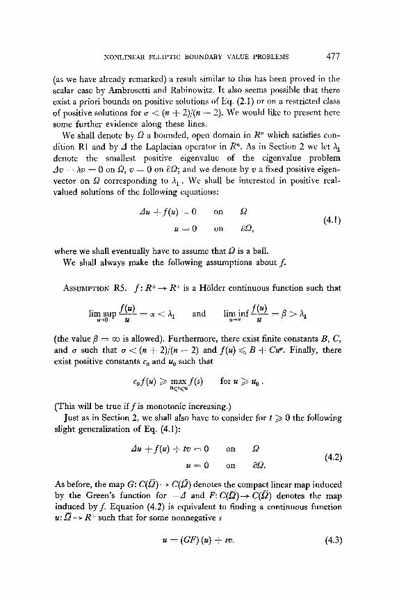
(as we have already remarked) a result similar to this has been proved in the scalar case by Ambrosetti and Rabinowitz. It also seems possible that there exist a priori bounds on positive solutions of Eq. (2.1) or on a restricted class of positive solutions for (T < (n + 2)/(n - 2). We would like to present here some further evidence along these lines.

We shall denote by D a bounded, open domain in R’” which satisfies condition Rl and by d the Laplacian operator in R”. As in Section 2 we let h, denote the smallest positive eigenvalue of the eigenvalue problem Av + hv = 0 on Q, v = 0 on 3Q; and we denote by v a fixed positive eigenvector on Sz corresponding to h, . We shall be interested in positive real- valued solutions of the following equations:

duff(u)=0 on Q

u = 0 on &Q, (4-l)

where we shall eventually have to assume that D is a ball. We shall always make the following assumptions about j.

ASSUMPTION R5. f: R+ ---f R+ is a Holder continuous function such that

lim sup f(u) = a < h, and u-0 u

liminfy =/I >h, u-+oD

(the value j3 = co is allowed). Furthermore, there exist finite constants B, C, and 0 such that u < (n + 2)/(n - 2) and f(u) 0 the following

slight generalization of Eq. (4.1):

Au+f(u)+tv=O on D

u =0 on ai2. (4.2)

As before, the map G: C(a) --f C(Q) denotes the compact linear map induced by the Green’s function for --d and F: C(D)+ C(D) denotes the map induced by f. Equation (4.2) is equivalent to finding a continuous function u: g + R+ such that for some nonnegative s

u = (GF) (u) + set. (4.3)

478 ROGER NUSSBAUM

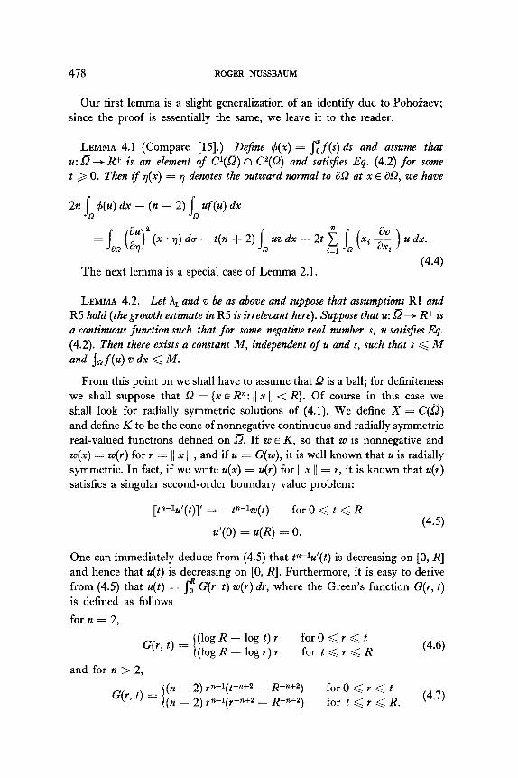
Our first lemma is a slight generalization of an identify due to Pohoiaev; since the proof is essentially the same, we leave it to the reader.

LEMMA 4.1 (Compare [15].) Dejke 4(x) = Jzf(s) ds and assume thut u: a -+ R+ is an element of Cl(a) n P(Q) and satisjies Eq. (4.2) for some t > 0. Then ;f T(X) = 7 denotes the outward normal to XJ at x E i32, we have

2n 1, W dx - (n - 2) jn uf (4 dx

= s, ($)” (x .71) da - t(n + 2) j. uv dx - 2t il s, (xi 2) u dx. z

The next lemma is a special case of Lemma 2.1. (4.4)

LEMMA 4.2. Let A, and v be as above and suppose that assumptions Rl and R5 hold (the growth estimate in R5 is irrelevant here). Suppose that u: 0 + R+ is a continuous function such that for some negative real number s, u satisjies Eq. (4.2). Then there exists a constant M, independent of u and s, such that s < M and s0 f (u) v dx < M.

From this point on we shall have to assume that Q is a ball; for definiteness we shall suppose that 52 = {x E R”: j/ x 11 < R). Of course in this case we shall look for radially symmetric solutions of (4.1). We define X = C(a) and define K to be the cone of nonnegative continuous and radially symmetric real-valued functions defined on D. If w E K, so that w is nonnegative and w(x) = w(r) for r = I[ x 11 , and if u = G(w), it is well known that u is radially symmetric. In fact, if we write u(x) = u(r) for 11 x 11 = r, it is known that u(r) satisfies a singular second-order boundary value problem:

[t”-124’(t)]’ = - tn-lw(t) for0 < t < R

u’(0) = u(R) = 0. (4.5)

One can immediately deduce from (4.5) that t”-%‘(t) is decreasing on [0, R] and hence that u(t) is decreasing on [0, R]. Furthermore, it is easy to derive from (4.5) that u(t) = sf G(r, t) w(r) d r, where the Green’s function G(r, t) is defined as follows

for n = 2,

(log R - log t) r G(r’ t, = [(log R - log r) r

for0 <r < t for t<r<R (4.6)

and for n > 2, (n - ‘4 +-l(t--n+2 - R--n+2

G(r9 t, = I(n _ 2)rn-l(r--n+2 _ R-n+; for0 <r < t for t < r < R. (4.7)

NONLIKEAR ELLIPTIC BOUNDARY VALUE PROBLEMS 479

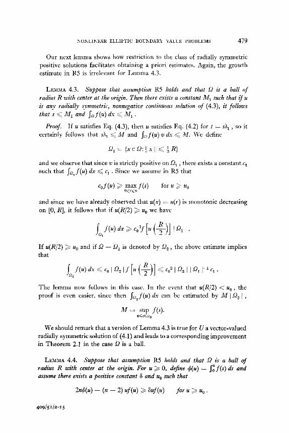
Our next lemma shows how restriction to the class of radially symmetric positive solutions facilitates obtaining a priori estimates. Again, the growth estimate in R5 is irrelevant for Lemma 4.3.

LEMMA 4.3. Suppose that assumption R5 holds and that 9 is a ball of

radius R with center at the origin. Then there exists a constant MI such that if u is any radially symmetric, nonnegative continuous solution of (4.3), it follows that s < MI and sn f (u) dx < 111, .

Proof. I f u satisfies Eq. (4.3), then u satisfies Eq. (4.2) for t = sX, , so it certainly follows that sh, < M and jnf (u) v dx < M. We define

and we observe that since z, is strictly positive on Q, , there exists a constant c, such that so, f (u) dx < c, . Since we assume in R5 that

and since we have already observed that U(X) = U(T) is monotonic decreasing on [0, R], it follows that if u(R/2) > u,, we have

s,, f (4 dx 2 c,lf [u (;-)I I Q, I . I f u(R/2) > u0 and if Q - Q, is denoted by .Qa , the above estimate implies

that

The lemma now follows in this case. In the event that u(R/2) < uO, the proof is even easier, since then JO,f(u) dx can be estimated by M j L?, I ,

M = ,~s&f (4.

We should remark that a version of Lemma 4.3 is true for U a vector-valued radially symmetric solution of (4.1) and leads to a corresponding improvement in Theorem 2.1 in the case Sz is a ball.

LEMMA 4.4. Suppose that assumption R5 holds and that Q is a ball of radius R with center at the origin. For u > 0, defke q%(u) = St f (s) ds and assume there exists a positive constant 6 and u0 such that

2n$(u) - (n - 2) uf (u) > Suf (u) for u >, uO .

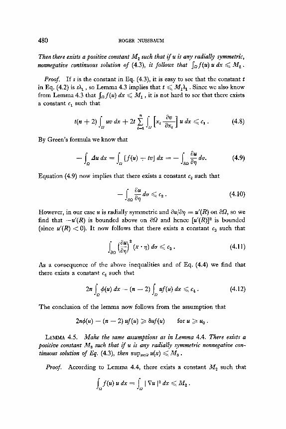
480 ROGER NUSSBAUM

Then there exists a positive constant M, such that if u is any radially symmetric, nonnegative continuous solution of (4.3), it follows that sn f (u) u dx < M, .

Proof. Ifs is the constant in Eq. (4.3), it is easy to see that the constant t in Eq. (4.2) is sh, , so Lemma 4.3 implies that t < MIXI . Since we also know from Lemma 4.3 that jof(u) dx < MI , it is not hard to see that there exists a constant c1 such that

t(n + 2) j, uv dx + 2t i j [xi $-] u dx < c1 . (4.8) i=l a 2

By Green’s formula we know that

- Audx= I s-2 j, [f(u) + 4 dx = - jan 2 da.

Equation (4.9) now implies that there exists a constant c2 such that

However, in our case u is radially symmetric and au/aq = u’(R) on Z’2, so we find that -u’(R) is bounded above on aQ and hence [u’(R)12 is bounded (since u’(R) < 0). It now follows that there exists a constant ca such that

au 2 IO q (x * rl) da < ~3 . ara

(4.11)

As a consequence of the above inequalities and of Eq. (4.4) we find that there exists a constant cp such that

22 S,+(u) dx - (n - 2) ja uf (u) dx G ~4 . (4.12)

The conclusion of the lemma now follows from the assumption that

2nfj(u) - (n - 2) uf (u) 3 *uf (u) for u > ua .

LEMMA 4.5. Make the same assumptions as in Lemma 4.4. There exists a positive constant MS such that if u is any radially symmetric nonnegative con-

tinuous solution of Eq. (4.3), then supzED u(x) < M, .

Proof. According to Lemma 4.4, there exists a constant M, such that

S,f(u) u dx = s, I Vu I2 dx < M2 .


If p = 2n/(n - 2) for n > 2 and if p is taken such that p > u and p 2 1 in the case n = 2, it follows from the Sobolev imbedding theorem that there exists a constant c, such that

The lemma now follows from Lemma 2.5. I

THEOREM 4.1. Suppose that Q is a ball of radius R and that assumption R5 holds. In addition, assume that there exist positive constants 6 and u. such that

2n+(u) - (n - 2) uf(u) > Suf (u) for u > uO , where d(u) = jzf(s) ds. There exist positive constants a and A such that if u is a nonnegative continuous radially symmetric solution of u = (GF) (u) (th a is, u is a classical solution of Eq. (4.2)), t

then u is identically zero or a < j/ u 11 = supzen 1 u(x)1 < A. Furthermore, if K denotes the cone of nonnegative continuous and radially symmetric real-valued

functions on Q and W = {u E K: a < 11 u I/ < A}, it follows that i,(GF, W) = - 1 and GF has a fixed point in W. In particular, Eq. (4.2) has a radially symmetric solution which is positive on L?.

Proof. According to Lemma 4.5, there exists a constant A such that all solutions u E K of the equation u = GF(u) + sv for some s > 0 satisfy

11 u 1) < A. Lemma 2.6 implies that there exists a positive constant a such thatifuEKandO<))u/I~a,onehasu#tGF(u)forO~tdl.Theorem 1.1 thus implies that i,(GF, W) = - 1 and GF has a fixed point in W. 1

The question of whether there exist a priori bounds for all positive scalar solutions of (4.1) (or perhaps for some nice subclass of all positive scalar solutions) for general Q and for o < (R + 2)/(n - 2) remains unanswered.

REFERENCES

1. H. AMANN, On the number of solutions of nonlinear equations in ordered Banach spaces, J. Functional Analysis 11 (1972), 346-384.

2. A. AMBROSETTI AND P. RABINOWITZ, Dual variational methods in critical point theory and applications, J. Functional Analysis 14 (1973), 349-381.

3. M. BERGER, “Stationary states for a nonlinear wave equation, J. Mathematical Phys. 11 (1970), 2906-2912.

4. G. M. GONCHAROV, On some existence theorems for the solutions of a class of nonlinear operator equations, Mat. Zametki. 7 (1970), 229-237.

5. J. D. HAMILTON, Noncompact mappings and cones in Banach spaces, Arch. Rational Mech. Anal. 48 (1972), 153-162.

6. M. A. KRASNOSELSKII, Fixed points of cone-compressing or cone-extending operators, So&t Math. Dokl. 1 (1960), 1285-1288.

482 ROGER NUSSBAUM

7. M. A. KRASNOSELSKII, “Positive Solutions of Operator Equations,” Noordhoff, Groningen, 1964.

8. M. G. KREIN AND M. A. RUTMAN, “Linear operators leaving invariant a cone in a Banach space,” Amer. Math. Sot. Translation No. 26 (series 1).

9. C. KURATOWSKI, Sur les espaces complets, Fund. Math. 15 (1930), 301-309. 10. C. MIRANDA, “Partial Differential Equations of Elliptic Type,” Springer-Verlag,

New York, 1970. 11. R. D. NUSSBAUM, The fixed point index and asymptotic fixed point theorems for

k-set-contractions, Bull. Amer. Math. Sot. 15 (1969), 490-495. 12. R. D. NUSSBAUM, The fixed point index for local condensing maps, Ann. Mat.

Pura A@. 89 (1971), 217-258. 13. R. D. NUSSBAUM, Periodic solutions of some nonlinear autonomous functional

differential equations, II, J. Differential Equations 14 (1973), 360-394. 14. R. D. NUSSBAUM, Periodic solutions of some autonomous functional differential

equations,” Ann. Mat. Pura Appl. 101 (1974), 263-306. 15. S. I. POHOZAEV, Eigenfunctions of du + hf(u) = 0, Soviet Math. Dokl. 6 (1965),

1408-1411. 16. P. RABINOWITZ, Some global results for nonlinear eigenvalue problems, J. Func-

tional Analysis 7 (1971), 487-513. 17. J. SCHWARTZ, “Nonlinear Functional Analysis, ” Courant Institute of Mathematic-

al Sciences, New York, 1965. 18. G. STAhlPACCHIA, “Equations Elliptiques du Second Ordre a Coefficients Discon-

tinus,” Les Presses de 1’Universite de Montreal, Montreal, 1966. 19. E. STEIN, “Singular Integrals and Differentiability Properties of Functions,”

Princeton University Press, Princeton, New Jersey, 1970. 20. A. ZYGMUND, “Trigonometric Series, I,” Cambridge University Press, London,

1959.

Date post:	23-May-2018
Category:	Documents
Upload:	vuongkiet
View:	218 times
Download:	1 times

Positive Solutions of Nonlinear Elliptic Boundary Value ... · JOURNAL OF MATHEMATICAL ANALYSIS AND...

Documents