Building Solutions to Nonlinear Elliptic and Parabolic Partial Differential Equations Adam Oberman University of Texas, Austin http://www.math.utexas.edu/~oberman Fields Institute Colloquium January 21, 2004
Transcript
Building Solutions to Nonlinear Elliptic and
Parabolic Partial Differential Equations
Adam Oberman
University of Texas, Austin
http://www.math.utexas.edu/~oberman
Fields Institute Colloquium
January 21, 2004
Early History of PDEs
Early PDEs
• Wave equation, d’Alembert 1752, model for vibrating string
• Laplace equation, 1790, model for gravitational potential
• Heat equation, Fourier, 1810-1822
• Euler equation for incompressible fluids, 1755
• Minimal surface equation, Lagrange, 1760
• Monge-Ampere equation by Monge, 1775
• Laplace and Poisson, applied to electric and magnetic problems:
Poisson 1813, Green 1828, Gauss, 1839
Solution methods were introduced
• separation of variables,
• Green’s functions,
• Power Series,
• Dirichlet’s principle.
H. Poincarre
An influential paper by H. Poincare in 1890, remarked that a wide variety
of problems of physics:
• electricity,
• hydrodynamics,
• heat,
• magnetism,
• optics,
• elasticity, etc. . .
have“un air de famille” and should be treated by common methods.
Stressed the importance of rigour despite the fact that the models are
only an approximation of physical reality. Justified rigour
• For intrinsic mathematical reasons
• Because PDEs may be applied to other areas of math.
Nonlinear PDE and fixed point methods
Picard and his school, beginning in the early 1880’s, applied the method
of successive approximation to obtain solutions of nonlinear problems
which were mild perturbations of uniquely solvable linear problems.
S. Banach 1922, fixed point theorem:
In a complete metric space X, a mapping S : X → X which satisfies
‖S(x) − S(y)‖ < K‖x − y‖, for all x, y ∈ X, and for K < 1,
has a unique fixed point.
Modern theory: non-constructive
Prior to 1920: classical solutions, constructive solution methods.
The development around 1920s of
1. Direct methods in calculus of variations.
(Classical spaces not closed: weak solutions lie in the completion.)
2. Approximation procedure used to construct a solution.
(Approximate solutions no longer classical.)
Led to notion of weak solution.
New methodology, separated issues of
i. Existence of weak solution
ii. Uniqueness of weak solution
iii. Regularity of weak solution
but no longer had
iv. Explicit construction of solutions
R. Courant, K. Freidrichs, H. Lewy 1928
Seminal paper in numerical analysis, predated computers.
Constructive solution methods for classical linear PDEs of math physics:
• elliptic boundary value and eigenvalue,
• hyperbolic initial value,
• parabolic initial value.
The finite difference method:
• replace differentials by difference quotients on a mesh.
• Obtain algebraic equations, construct solutions to these equations.
• Prove convergence (in L2 norm).
Elliptic PDE: implicit scheme.
Hyperbolic/Parabolic PDE: explicit scheme
but with restriction on the time step, (the CFL condition.)
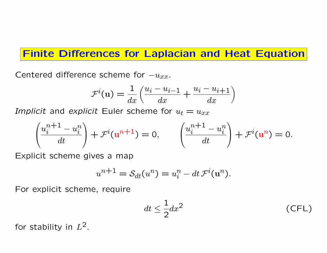
Finite Differences for Laplacian and Heat Equation
Centered difference scheme for −uxx.
F i(u) =1
dx
(
ui − ui−1
dx+
ui − ui+1
dx
)
Implicit and explicit Euler scheme for ut = uxx
un+1i − un
i
dt
+ F i(un+1) = 0,
un+1i − un
i
dt
+ F i(un) = 0.
Explicit scheme gives a map
un+1 = Sdt(un) = un
i − dtF i(un).
For explicit scheme, require
dt ≤1
2dx2 (CFL)
for stability in L2.
Convergence of Approximation methods
Lax-Richtmeyer 1959, stability necessary for convergence of linear dif-
ference schemes in L2.
Lax Equivalence theorem a “Meta-theorem” of Numerical Analysis:
Consistent, stable schemes are convergent.
Need to make these notions precise to get a theorem,
in particular, need to assign a norm for stability.
For nonlinear or degenerate PDE, the solutions may not be smooth.
It is essential for convergencethat the norm used in the existence and uniqueness theory
be the norm used for stability of the approximation.
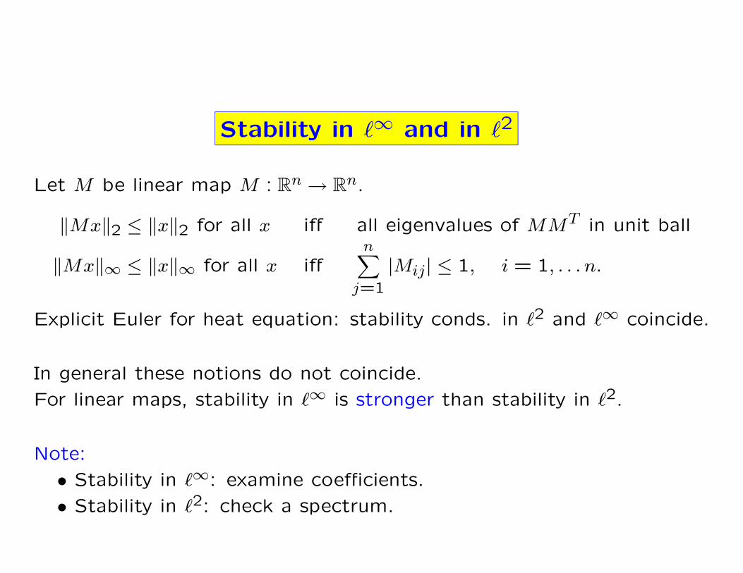
Stability in ℓ∞ and in ℓ2
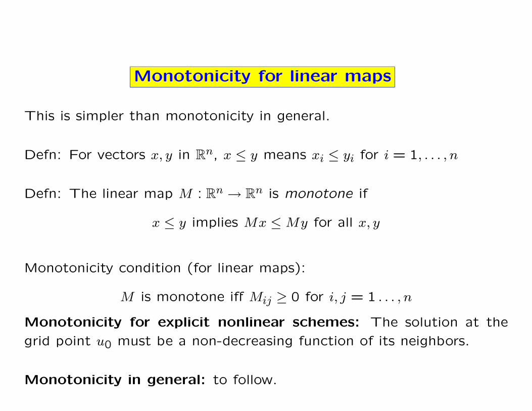
Let M be linear map M : Rn → Rn.
‖Mx‖2 ≤ ‖x‖2 for all x iff all eigenvalues of MMT in unit ball
‖Mx‖∞ ≤ ‖x‖∞ for all x iffn
∑
j=1
|Mij| ≤ 1, i = 1, . . . n.
Explicit Euler for heat equation: stability conds. in ℓ2 and ℓ∞ coincide.
In general these notions do not coincide.
For linear maps, stability in ℓ∞ is stronger than stability in ℓ2.
Note:
• Stability in ℓ∞: examine coefficients.
• Stability in ℓ2: check a spectrum.
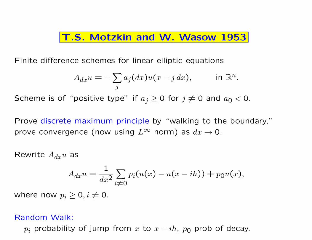
T.S. Motzkin and W. Wasow 1953
Finite difference schemes for linear elliptic equations
Adxu = −∑
j
aj(dx)u(x − j dx), in Rn.
Scheme is of “positive type” if aj ≥ 0 for j 6= 0 and a0 < 0.
Prove discrete maximum principle by “walking to the boundary,”
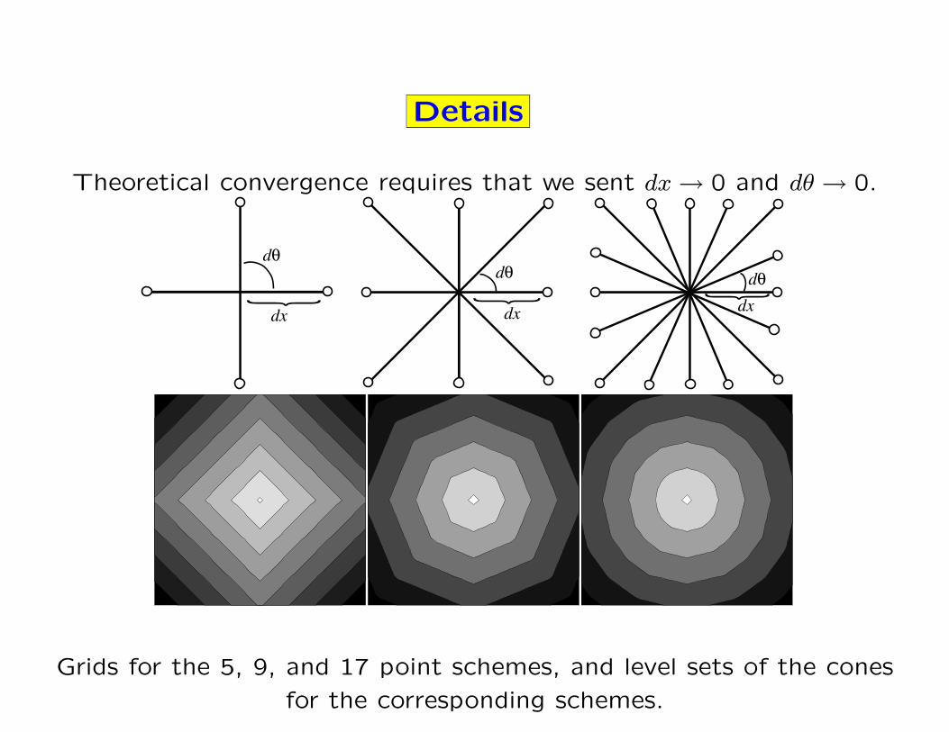
prove convergence (now using L∞ norm) as dx → 0.
Rewrite Adxu as
Adxu =1
dx2
∑
i6=0
pi(u(x) − u(x − ih)) + p0u(x),
where now pi ≥ 0, i 6= 0.
Random Walk:
pi probability of jump from x to x − ih, p0 prob of decay.
The Comparison Principle
Viscosity Solutions, Monotone schemes
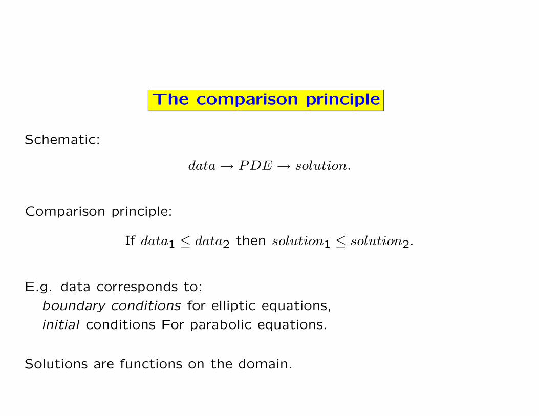
The comparison principle
Schematic:
data → PDE → solution.
Comparison principle:
If data1 ≤ data2 then solution1 ≤ solution2.
E.g. data corresponds to:
boundary conditions for elliptic equations,
initial conditions For parabolic equations.
Solutions are functions on the domain.
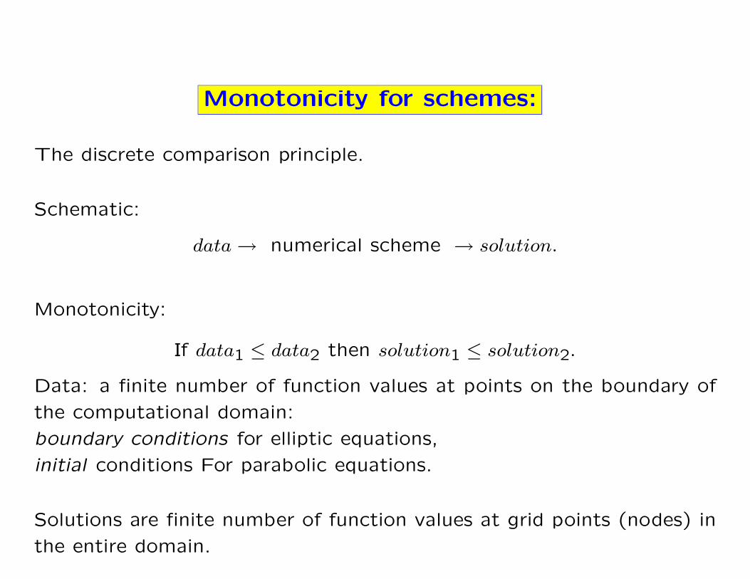
Monotonicity for schemes:
The discrete comparison principle.
Schematic:
data → numerical scheme → solution.
Monotonicity:
If data1 ≤ data2 then solution1 ≤ solution2.
Data: a finite number of function values at points on the boundary of
the computational domain:
boundary conditions for elliptic equations,
initial conditions For parabolic equations.
Solutions are finite number of function values at grid points (nodes) in
the entire domain.
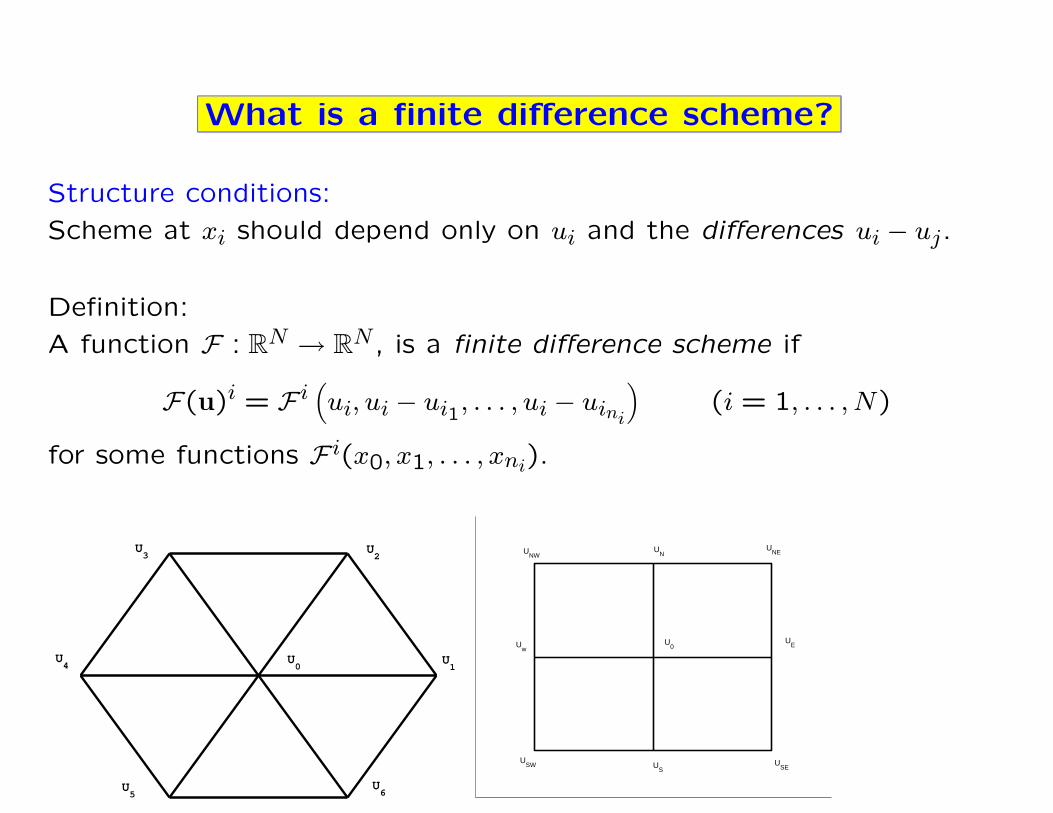
Local structure conditions
Local structure conditions on the PDE (degnerate ellipticity) ensures
that the comparison principle holds.
We find (A.O.) local structure conditions on the numerical schemes
which ensures that monotonicity holds. Furthermore, this structure
condition leads to
• self-consistent existence and uniqueness proofs for solutions of the
scheme,
• an explicit iteration scheme which can be used to find solutions.
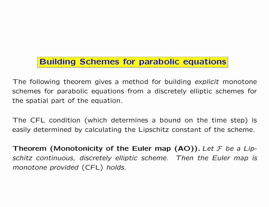
Elliptic equations lead to implicit schemes, whereas explicit, monotone
schemes for parabolic equations can be built from the scheme for the
underlying elliptic equation.
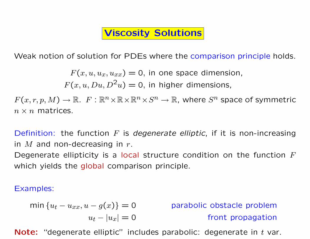
Viscosity Solutions
Weak notion of solution for PDEs where the comparison principle holds.
F (x, u, ux, uxx) = 0, in one space dimension,
F (x, u, Du, D2u) = 0, in higher dimensions,
F (x, r, p, M) → R. F : Rn×R×Rn×Sn → R, where Sn space of symmetric
n × n matrices.
Definition: the function F is degenerate elliptic, if it is non-increasing
in M and non-decreasing in r.
Degenerate ellipticity is a local structure condition on the function F
which yields the global comparison principle.
Examples:
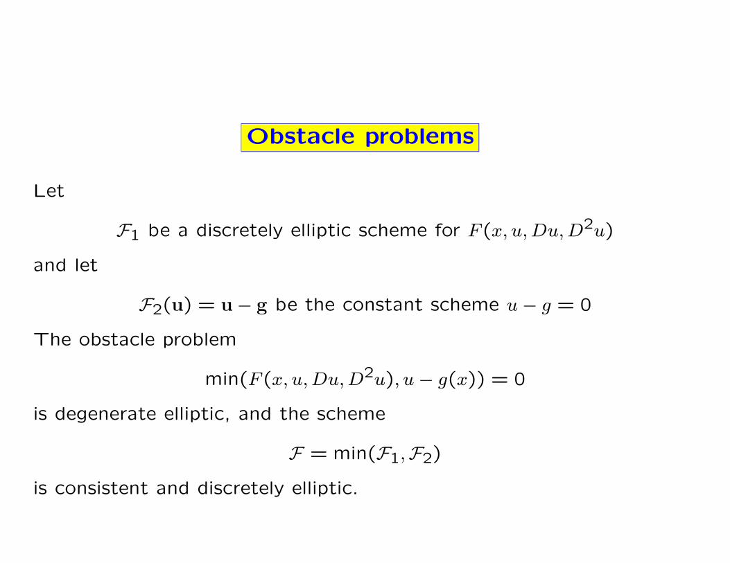
min ut − uxx, u − g(x) = 0 parabolic obstacle problem
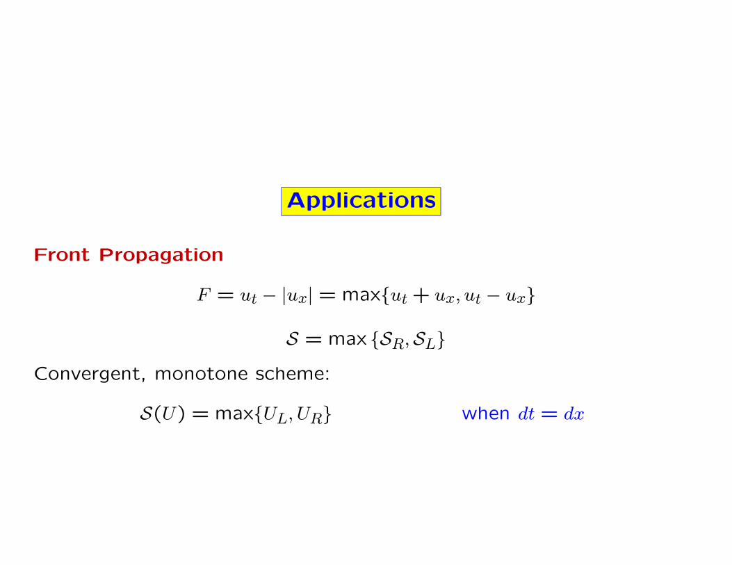
ut − |ux| = 0 front propagation
Note: “degenerate elliptic” includes parabolic: degenerate in t var.
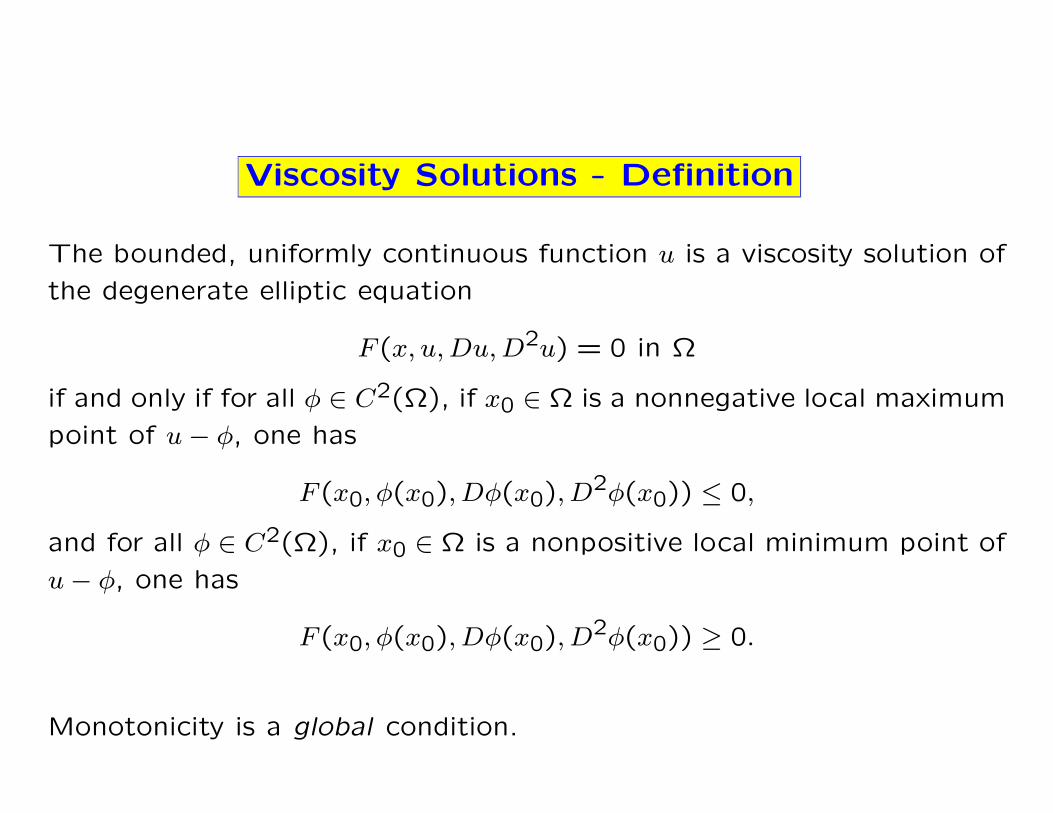
Viscosity Solutions - Definition
The bounded, uniformly continuous function u is a viscosity solution of
the degenerate elliptic equation
F (x, u, Du, D2u) = 0 in Ω
if and only if for all φ ∈ C2(Ω), if x0 ∈ Ω is a nonnegative local maximum
point of u − φ, one has
F (x0, φ(x0), Dφ(x0), D2φ(x0)) ≤ 0,
and for all φ ∈ C2(Ω), if x0 ∈ Ω is a nonpositive local minimum point of
u − φ, one has
F (x0, φ(x0), Dφ(x0), D2φ(x0)) ≥ 0.
Monotonicity is a global condition.
Existence and Uniqueness of Viscosity Solutions
M. Crandall, P.L. Lions, G. Barles, L.C. Evans, H. Ishii, P.E. Souganidis
Theorem. For a wide class of degenerate elliptic equations there exist
unique viscosity solutions.
Viscosity solutions are the correct framework for proving existence and
uniqueness results for PDE for which the Comparison Principle holds.
Convergence of Approximation Schemes
G. Barles and P.E. Souganidis (1991)
Theorem.The solutions of a stable, consistent, monotone scheme con-
verge to the unique viscosity solution of the PDE.
Q: Does it really matter if the schemes are not monotone?
Q: How do we find monotone schemes?
End of introduction
To follow:
definitions, and theorems regarding: building monotone schemes.
Results for
• Math Finance, HJ equations
• Nonconvergent methods
• Convergent schemes for motion by mean curvature, infinity laplacian
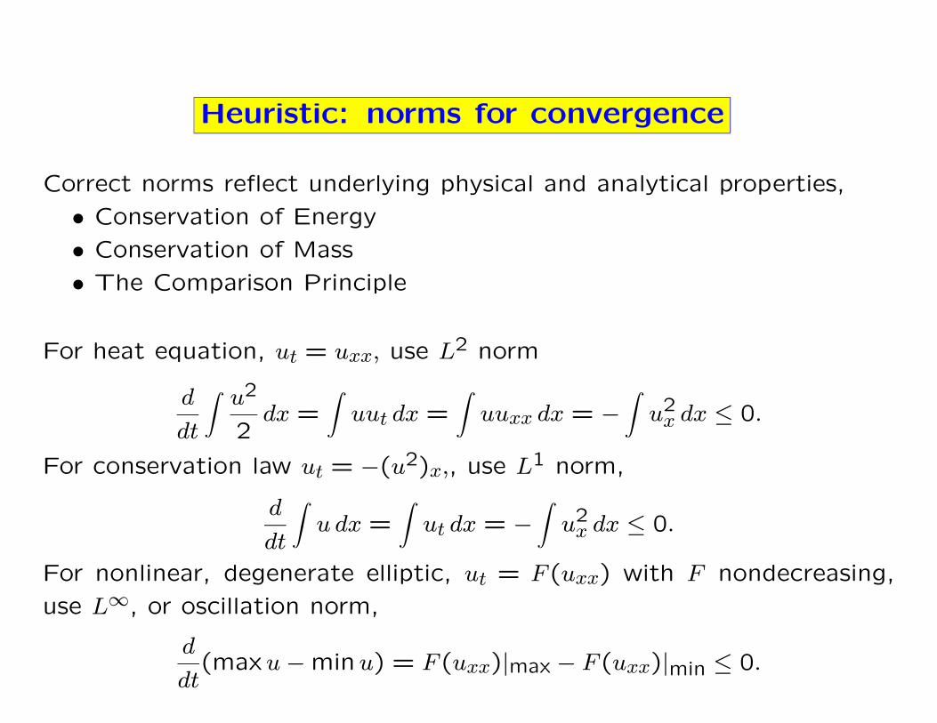
Heuristic: norms for convergence
Correct norms reflect underlying physical and analytical properties,
• Conservation of Energy
• Conservation of Mass
• The Comparison Principle
For heat equation, ut = uxx, use L2 norm
d
dt
∫
u2
2dx =
∫
uut dx =∫
uuxx dx = −∫
u2x dx ≤ 0.
For conservation law ut = −(u2)x,, use L1 norm,
d
dt
∫
u dx =∫
ut dx = −∫
u2x dx ≤ 0.
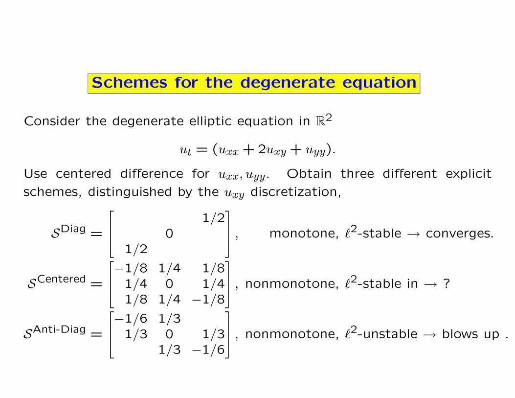
For nonlinear, degenerate elliptic, ut = F (uxx) with F nondecreasing,
use L∞, or oscillation norm,
d
dt(maxu − minu) = F (uxx)|max − F (uxx)|min ≤ 0.
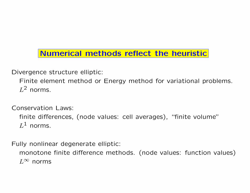
Numerical methods reflect the heuristic
Divergence structure elliptic:
Finite element method or Energy method for variational problems.