U.U.D.M. Project Report 2013:22

Examensarbete i matematik, 15 hpHandledare och examinator: Johan TyskJuni 2013

A Comparison of Models for Oil Futures

Hayat Haseeb

Department of MathematicsUppsala University

  2  

Abstract

In this paper we have shown and compared two oil futures term structure models, namely

the famous Gabillon 1991 two-factor model and Cortazar and Schwartz 2003 three-factor

model. A thorough mathematical presentation of the models was offered and their

essential backgrounds were explained. Each model has shown to have its advantages and

disadvantages in terms of calibration and results. The Cortazar and Schwartz model

proved to be a better fit although both models are able to accurately predict future oil

price movements. Essentially, both models focus on the long-term price factor to

ultimately model the term structure curve.

  3  

Table of Contents

1. Introduction 4 1.1 The Oil Futures Market 5 1.2 Understanding Forwards and Futures 8

2. The Pricing of Oil Futures 12

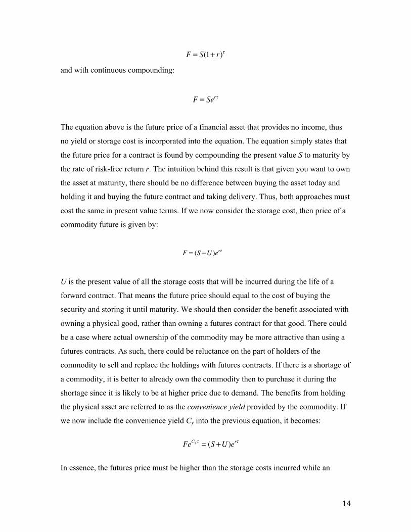
2.1 The Theory of Storage hypothesis 13 2.2 The Risk Premium hypothesis 15

3. Oil Pricing Models 17 3.1 General Modeling Method 18 3.2 The Diffusion Processes 20

4. The Term Structures of Oil Futures 22

4.1 The Spot and Futures Price 22 4.2 Features of the Term Structure of Oil Futures 23

5. Gabillon and Schwartz Models of Oil Futures 26 5.1 Gabillon 1990 two-factor 26 5.2 Cortazar and Schwartz 2003 three-factor model 39

6. Comparison of the Two Models 45

6.1 Modeling approach 45 6.2 Calibration 50 6.3 Results 51

7. Conclusion 55

8. Summary 56

9. References 57

 

  4  

1. Introduction

There has been a massive development of financial products in oil markets and in the

mathematics behind such transactions in the last 20 years. Oil futures have become

increasingly important in the world of finance, reaching a record sum of 26 billion dollars

in traded futures in April of 2011. Today, approximately 1.3 trillion barrels of crude oil

exist in the world, making oil the most heavily traded commodity. Because of oils huge

liquidity and the many types oil futures for investors to choose from, speculative oil

trades are more popular now than ever before.

Much interest remains in understanding how oil futures prices evolve not only over time

but also across maturities. The term structures of oil futures is defined as the relationship

between the spot price and futures price for some future delivery date. Term structure

models of futures prices aim to reproduce the futures prices observed in the market as

accurately as possible. The term structure is of particular importance to investors because

its shape indicates the supply and demand characteristics of oil and serves as a good

investment guide for investing in oil and consequently, for trading its futures contracts.

There have been extensive studies and many oil-specialized models that aim to describe

the term structure of futures prices where several authors have observed that a number of

factors are important in describing the changes in the futures curve. In this paper we will

be focusing on two models for the term structure of oil futures prices – the well-known

Gabillon (1990) two-factor model and the widely studied Cortazar and Schwartz (2003)

three-factor model. Gabillon and Schwartz models are the most popular in researchers

and market practitioners, not only because their appropriate interpretation on convenience

yield or long term price, but also because their simplicity and clarity. By inspecting these

models we will aim to answer two questions (i) can we provide a useful critical

interpretation of the different methodologies, and (ii) which model is a better predictor of

future price?

  5  

In this Section, we will begin with an overview of the oil markets, and then move onto

explaining the features of forwards and futures, and there in the basic terminology that

this paper is dealing with. The rest of this paper is organized as follows: Section 2 centers

around explaining the notions behind the pricing mechanisms of futures. Section 3

provides an understanding of the general modeling method. Section 4 describes the

concepts involved in the term structure of oil futures prices. In Section 5 we gradually

introduce and analyze the construction of the two models. Section 6 constitutes the main

part of this paper where we compare the two models, as well as scrutinize and offer

insight. Section 7 concludes this paper and finally, Section 8 offers a summary.

1.1 The Oil Futures Markets

At the most basic level, oil futures are instruments that allow investors to purchase or sell

a specific number of units of oil at a specific price on a specific day. We will deal with a

deeper and more detailed understanding of futures contract in the forthcoming sections

(where will also see that the majority of oil futures trading does not involve ownership of

the actual oil). The essentials of crude oil futures trading are a confusing subject to the

general population, but the effects are widely felt financially. But what exactly is the oil

futures market? and why is it relevant? In this segment we aim to answer these questions

among others. Before delving into the description of the oil futures market, some basics

about oil as a commodity are looked at to gain to some insight into the scope of the oil

industry. We will also look at the trading oil futures, mechanisms of the market, and

general market trends.

Oil as a Produce

Oil, as mentioned earlier, is arguably the world’s most important commodity and the

most traded commodity in the world when it comes to futures contracts. Oil itself is not

an end product, and therefore there is no direct demand for it. Instead, the demand

concerns its various products. Roughly 43% of each barrel of oil (wher one barrel is

approximetly 160 liters) is used for automobile fuel; 23% is used for diesel and heating

  6  

oil; 9% is used for jet fuel; 3.8% is used for electrical power generation; and the rest is

used for petrochemicals and lubricants. The major oil producing countries are Saudi

Arabia (13% of world production), Russia (12%), the United States (7%), Iran (6%) and

China (5%).

Although publicly traded international oil companies are viewed as the dominant players

in the oil market, state-owned national oil companies actually account for a much larger

share of reserves and production. The two largest oil-producing companies in the world

are Saudi Aramco and the National Iranian Oil Company, who account for around

12 per cent and 5 per cent of global oil production, respectively. In total, national oil

companies control around 60 per cent of oil production and more than 80 per cent of the

world's proven oil reserves. The five largest publicly traded oil-producing companies (the

‘super-majors’) – Exxon Mobil, BP, Chevron, Royal Dutch Shell and Total – each

account for around 2–3 per cent of global oil production and collectively just 3 per cent

of reserves.

As of September 2012, global demand for oil is estimated at 90.2 million barrels of oil

per day. That comes out to 32.9 billion barrels per year. Right now, supply is at or

slightly above that number, but in the future, if demand continues to rise as expected,

supply could become constrained. The issue of “peak oil” – the date at which half of the

reserves existing at the beginning of time will be consumed – is the subject of intense

debates. The concern of depleting reserves in the context of an exhaustive commodity

such as oil is certainly present on market participants’ minds. Current predictions suggest

that the world oil supply should last until 2045.

Oil futures trading

There are more than 300 different types of crude oil produced around the world, all of

which have different characteristics. However, there are only four main types oil futures

that are traded; these are the Light Sweet Crude Oil (also known as the West Texas

Intermediate or WTI) futures, Brent Crude Oil futures, Heating Oil futures and the Gasoil

  7  

futures. The most actively traded is the Light Sweet Crude Oil future (the name is due to

its a low sulfur content), and is preferred by oil traders for its high liquidity. The main oil

futures exchanges are the New York Mercantile Exchange (NYMEX) and the

Intercontinental Exchange (ICE). In 2011 the ICE reached record volumes of 33 million

contracts during one month, while the NYMEX reached records averaging 2.2 million

contracts a day. The WTI contracts then averaged a daily volume of 935,000 contracts

while the Brent Crude oil futures averaged 576,000 contracts a day.

All oil futures contracts are traded on a regulated futures exchange i.e. a central

marketplace where futures contracts are listed. However, only around 1 per cent of these

contracts are in fact settled in terms of the physical commodities (we will explain why

this is so in the next segment). These contracts are always standardized in terms of the

type of oil (since crude oil around the world varies in its hydrocarbon makeup and the

relative cost of delivery and transport). Oil futures are listed for trading in every month of

the year for the current year and at least three more years into the future. Although there

are important exceptions, the most trading volume is typically concentrated in the front-

month contract, which is the contract nearest to maturity.

There is actually no specific individual market price for most physical oils. Instead,

prices are determined with reference to a few benchmark oil futures prices (so-called

"marker crudes"), notably Brent and West Texas Intermediate. Oil prices quoted by the

press on a daily basis usually refer to prices of nearest maturity future contract instead of

the actual spot price of oil (the price of buying or selling the oil today). This means, oil is

not traded on the spot markets but on the futures market instead. Spot prices must be then

estimated on the basis of futures prices because spot prices are not an observable

variable. This is the reason why the nearest futures contract is considered a “proxy” to the

spot price i.e. futures prices are the reference for spot oil prices.

  8  

Market trends and impact

Most traders of oil futures traders predict that the price of oil is going to rise in the future,

so if they purchase oil futures at a low current rate, they'll have turned a profit when the

price of oil actually does rise in the future. However, if they were wrong and the price of

oil drops, oil futures traders would lose money. The price of oil has risen by about 60%

since mid-2004 and by more than 40% since the beginning of 2005. Although economies

tend to absorb supply shocks, the path of future oil prices remains a concern for monetary

policymakers. Higher oil prices can damp demand, as consumers and firms spend more

of their budgets on oil-related products and less on other goods and services.

Furthermore, if higher oil prices are passed through to a significant extent to other goods

and services and ultimately wages, inflationary pressures can build. In June 2008 oil

prices experienced a steady upward trend; reaching $147 a barrel to then dramatically fall

in December 2008 to $30 per barrel. Many believe that these swings had to do with the

role of speculative traders in the crude oil market. With the exception of 2008 to 2009,

when a global recession was in full swing, global oil consumption has steadily increased

for decades over the long run.

1.2 Understanding Forwards and Futures

To fully understand futures one needs to also look at its much simpler counterpart i.e.

forwards. Forward contracts allow people to buy or sell a specific type of asset at a

specific time at a given price. It is in the specific differences between forward and futures

that will enable us to understand futures. These differences will highlight the main

features of the futures contract and are described below. To gain a better understanding of

forwards and futures we will begin by taking a brief look at their history.

  9  

History of Forward and Futures

The history of forward contracts dates back to ancient times. Due to the difficulty of

transporting goods at the time, trading based on samples was common. After a sample

was delivered, and to ensure both parties would honor the deal once the good was

transported, some form of contract was essential and forward contracts were established.

Futures appeared because a more standardized form of a forward contract was needed as

well as a venue where prices could be listed and communicated. This began in 1958 at

the Chicago Board of Trade exchange where members served as brokers who facilitated

trading in return for commission. The exchange allowed for there to be a specific

platform where merchants and farmers could trade corn forwards. As trading of corn

forwards increased, the Board decided that standardizing those contracts would

streamline the trading and delivery processes. This meant, instead of individualized corn

contracts, which took a long time to agree on and fulfill, people trading were asked to

trade contracts that were identical in terms of quantity, quality, delivery months and

terms, all as established by the exchange. The only thing left for traders to negotiate was

price and the number of contracts. These standardized contracts gave way for the first

futures contacts. Since transportation of corn was lengthy at the time, this form of

agreement allowed for merchants to avoid the risk of price of fluctuations as well. The

usefulness of futures then became apparent and a number of futures exchanges were

established throughout the country.

Features of Forwards and Futures

Today, futures are still traded on an exchange, while forwards are traded in over-the-

counter markets (a network of communicating dealers who do not physically meet).

Forwards are entirely customized by the parties and all the terms of the contract are

privately negotiated between parties. The underlying asset can be anything, at any

volume, any settlement date and any settlement form (cash or physical), which are also

entirely up to the parties of the forward contract. On the other hand, futures are fully

standardized and transacted through brokerage firms that hold a “seat” only on the

  10  

exchange that trades that particular contract. The terms of a futures contract - including

delivery places and dates, volume, technical specifications and trading and credit

procedures -are set for each type of contract. Two parties will work through their

respective brokers to transact a futures trade and can only trade futures contract that are

supported by each exchange.

The specific details and risk concerning settlement and delivery for forwards and futures

contracts are also quite distinct. Although the parties of a forward contract are always

prepared to bid or offer a price, the transaction is not always guaranteed. These risks have

to with the fact that forwards contracts are settled at the end of the contract on the

specific expiration date while settlement for futures can occur over a range of dates. This

settlement over a range of dates makes use of the marked-to-market daily process.

Marked-to-market insures that there is less risk for a party to default on its side of the

agreement (a major difference and advantage to forward contracts). It is essentially the

daily settling of the value of the futures contract to zero, until the end of the contract.

Every gain is exactly offset by a loss of the same amount, where traders are asked by

brokers to top up a loss (via transfers from their margin accounts) if the amount is

reduced to a certain level. Due to this, there no initial investment for futures contracts but

instead, a varying cash flow. Marked-to-market has an extremely big impact on futures

trading as it directly determines if the investor has gained or lost money for the day. In

contrast, profit or loss on forward contract can only be realized at the time of the

settlement. It is also important to note that the futures price is different from the value of

a futures contract. Upon entering a futures contract, no cash changes hands between

buyers and sellers – and hence the value of the contract is zero at its inception, and

continues to be so due to marked-to-market.

A futures contract can be regarded as a series of one-day forward contracts, where the

profit or loss is realized each day and a new contract is written at the current futures

price, or at the price that sets the value of the contract equal to zero. When the interest

rate is non-stochastic will futures and forward prices be equal. If the interest rate is

stochastic and is positively (negatively) correlated with the spot price of the underlying

  11  

commodity, the futures price will be greater (less) than the forward price. While forward

and futures prices can also differ because of different tax treatments, transaction costs or

margin rules, empirical research indicates that for most commodities and other traded

assets, even when the price difference is statistically significant, the magnitudes are small

and may not be significant economically.

The Role of Forwards and Futures

Forwards and futures prices are closely watched by a vast number of participants, where

many try to predict their future price movements. The role forwards and futures play is

essential to the evading of risk and locking in profit. We categorize two broad groups of

traders in the oil market: hedgers and speculators. Hedgers are people who actually want

to buy and sell oil, the physical commodity. These hedgers move around the product to

minimize the risk they might encounter based on market fluctuations. This means, the

hedger plans to buy (sell) oil, and buys (sells) a futures contract to lock in a price and

protect against rising (falling) prices. Speculators, on the other hand, don’t want to own

the oil at all but instead want to take on a bit of risk and possibly make some money by

betting on the future direction of oil. They buy in to future oil contracts, from the

hedgers, based on what they think the price of oil will be. Speculators earn a profit when

they offset futures contracts to their benefit. To do this, a speculator buys contracts then

sells them back at a higher (contract) price than that at which they purchased them.

Conversely, they sell contracts and buy them back at a lower (contract) price than they

sold them. n either case, if successful, a profit is made. This might seem to seem strange

that there are investor who would want to buy large quantities of something like oil but

not own it. But it is precisely because they don’t want to actually own the physical oil

that the oil futures market works.

  12  

2. The Pricing of Oil Futures

There has long been interest in understanding the pricing of futures commodity contracts.

This has led to the development of two major classes of valuation methods for futures

pricing, namely, the Theory of Storage (or Cost-of-Carry) and the Risk Premium (or

Unbiased Expectations) hypotheses. Both hypotheses have shown the relationship

between spot and futures prices and have now become an integral part in explaining term

structure of oil futures prices. The key difference between the two hypotheses is that one

is ”convenience yield based “and the other is “risk premium founded” although the initial

modeling set up, as we will see in the next section, tends to be fairly similar. Presenting

both hypothesis will help with the understanding our chosen models in subsequent

sections. We will also look at why one hypothesis may be preferred to other and why, but

first let’s begin with the necessary assumptions.

The market assumptions

It is assumed that markets under the both hypothesis do not permit arbitrage

opportunities. Arbitrage is the possibility for a riskless profit opportunity to be made in

trading. Allowing for arbitrage would mean an extreme form of market inefficiency since

it implies that two identical commodities trade at different prices. Assuming arbitrage

opportunities can never arise in the market should not be taken literally, but rather that

they cannot persist. That is, while a misalignment of prices may create such chances,

market participants take advantage of them as they arise, and prices always adjust to

eliminate the arbitrage.

The remaining assumptions assumed are as follows: the market participants are subject to

no transactions costs when they trade. Secondly, the market participants are subject to the

same tax rate on all net trading. And finally, the market participants can borrow money at

the same risk-free rate of interest as they can lend money.

  13  

3.2 The Theory of Storage hypotheses

The Theory of Storage hypothesis was first formalized by Kaldor (1939), Working (1984,

1949) and Brennan (1958). It takes into consideration that commodities have to be stored,

can be consumed and do deteriorate over time. In addition, commodity prices are affected

by changes in supply. To incorporate these ideas into the pricing of futures, the concept

of the convenience yield was introduced. We will offer a thorough explanation of the

concept of convenience yield as we proceed. We will see that The Theory of Storage

hypotheses is a very simple concept of futures pricing as it assumes that the futures price

depends only on the spot price and the convenience yield

Determining the price

It is essential to understand how the factors of the theory of storage hypothesis are

gradually introduced into the final pricing equation. This will enable us to understand the

construction of Gabillon’s preliminary models in section 5.

We will be using the following notions throughout this section:

S Spot Price

F Futures Price

t Current time

T Maturity

Time to maturity (T-t)

The commodity future price can be found using the same economic principles used for

financial asset future price, but the details will be different. Assuming constant rates, for

a simple, non-dividend paying financial asset, the value of the futures price F will be

found by compounding the present value the spot price S at time to maturity by the rate of

risk-free return r:

τ

  14  

and with continuous compounding:

The equation above is the future price of a financial asset that provides no income, thus

no yield or storage cost is incorporated into the equation. The equation simply states that

the future price for a contract is found by compounding the present value S to maturity by

the rate of risk-free return r. The intuition behind this result is that given you want to own

the asset at maturity, there should be no difference between buying the asset today and

holding it and buying the future contract and taking delivery. Thus, both approaches must

cost the same in present value terms. If we now consider the storage cost, then price of a

commodity future is given by:

U is the present value of all the storage costs that will be incurred during the life of a

forward contract. That means the future price should equal to the cost of buying the

security and storing it until maturity. We should then consider the benefit associated with

owning a physical good, rather than owning a futures contract for that good. There could

be a case where actual ownership of the commodity may be more attractive than using a

futures contracts. As such, there could be reluctance on the part of holders of the

commodity to sell and replace the holdings with futures contracts. If there is a shortage of

a commodity, it is better to already own the commodity then to purchase it during the

shortage since it is likely to be at higher price due to demand. The benefits from holding

the physical asset are referred to as the convenience yield provided by the commodity. If

we now include the convenience yield Cy into the previous equation, it becomes:

In essence, the futures price must be higher than the storage costs incurred while an

F = S(1+ r)τ

F = Serτ

F = (S +U )erτ

FeCYτ = (S +U )erτ

  15  

investor waits for maturity. If the futures price is too low, the investor holding the

commodity in inventory could sell the commodity on the spot market and buy the futures

contract to avoid the storing costs until the maturity of the futures contract. More distant

futures price equals nearby futures price plus cost of carry

If the marginal storage costs CC, known as the cost of carry, are included and we

rearrange the above equation, then the price is defined as:

Finally, this equation ties the subsequent concepts to represent the price of futures

contract under the Theory of Storage hypothesis.

3.2 The risk premium hypotheses

Keynes (1930) first introduced the concept of risk premium in commodity markets to

explain the behavior of speculators in The Theory of Normal Backwardation (which we

will explain further in Section 4). Oil futures prices reflect the price that both the buyer

and the seller agree will be the price of oil upon delivery. Therefore, these prices provide

direct information about investor’s expectations about the future price of oil. Like the

prices of every other risky asset, however, oil futures prices include risk premiums, to

reflect the possibility that spot prices at the time of delivery may be higher or lower than

the contracted price. The risk premium is the reward for holding a risky investment rather

than a risk-free one. More precisely, the risk premium is the difference between the spot

price forecast, which is the best estimate of the going rate of the commodity at some

specific time in the future, and the futures price, i.e. the actual price a trader is prepared

to pay today for delivery of the commodity in the future.

F = Se(r+CC−CY )τ

  16  

The equation for the futures price is the conditional expectation of the spot price

discounted at the appropriate continuously compounded risk premium rp :

The two valuation principles are mutually consistent if convenience yields are regarded

as the deviation of the commodity spot price from its asset value (the present value of the

expected commodity spot price at maturity). By combining risk-premium models and

convenience-yield models, it can be shown that convenience yields reflect the proportion

of the expected change in commodity spot prices which is not attributable to the risk

premium and the risk-free rate.

Ft = Et (ST )e−rpτ

  17  

3. Oil Pricing Models

The pricing and modeling of oil markets are far more complex than the modeling of

interest rate and equity markets since commodities are produced, consumed, transported

and stored causing wide swings of market inventory. The different number of

fundamental price drivers cause complex oil price behaviors and an unpredictable nature.

In this section we will explain the general pricing method employed to construct oil

pricing models and their various feature. We will also look at the common diffusion

processes employed in oil pricing models to gain a better understanding of the modeling

mechanism.

Characteristics Oil Prices

It is important to describe the actual behavior of the oil spot prices that we are trying to

model. Therefore, we will begin by doing this before starting with the description of the

mathematical models.

Oil prices tend to exhibit strong seasonal patterns in response to cyclical fluctuations in

supply and demand mostly due to weather and climate changes. Despite the sharp rises

during short periods of such specific events oil prices usually revert to a normal level.

This means, oil prices will fluctuate around and drift over time to values determined by

the cost of production and the level of demand.

The prices of oil can suddenly spike. This comes about when stored supplies are

exhausted, or when storage is full, or when the production capacity is exhausted. Oil

spikes present a particular modeling difficulty, because they are not like ordinary jumps

one would experience in, e.g. equity markets.

Based upon historical prices, market operators might have expectations about future price

development. Anticipated future supply/demand configurations, and guesses about moves

from influential oil producers such as OPEC, impact the market operators’ expectations

about future oil prices and alter the price.

  18  

3.1 General Modeling Method

The first valuation model to price derivatives on commodities can be attributed to

Black(1976) who derived the futures price formula of commodities by supposing the spot

price of commodities to follow a diffusion process as in the Black Scholes model. Since

then all oil pricing models have used this same underlying principle, as we will show

below. We will begin this segment with two key principles often encountered in the

construction oil pricing models.

Risk-neutral valuation and Replication

In a risk-neutral world all individuals are indifferent to risk. In such a world investors

require no compensation for risk, and the expected return on all securities is the risk-free

interest rate. The value of the future is its expected payoff in a risk-neutral world

discounted at the risk-free rate. This result is an example of an important general

principle in security pricing known as risk-neutral valuation. The principle states that we

can assume the world is risk neutral when pricing a future. The price we obtain is correct

not just in a risk-neutral world but in the real world as well.

Replication underlies that the pricing and hedging of all derivative securities is based on a

simple idea. The payoffs of a derivative are determined by changes in the price of the

underlying asset. Therefore, it should be possible to re-create these payoffs by directly

using the underlying asset and, perhaps, cash (borrowing or lending at the risk-free rate).

If such a portfolio can be constructed, it is called a replicating portfolio. The derivative

and its replicating portfolio lead, by definition, to identical outcomes, so, under the no-

arbitrage condition, they must have the same cost. The cost of the replicating portfolio is

readily computed since it consists of only the underlying spot asset and cash. Thus, the

cost of the derivative, its so-called “fair price,” is identified. The key step in exploiting

these ideas is identifying the composition of the replicating portfolio

  19  

Under risk neutrality and arbitrage free measure it is possible to continuously and

perfectly hedge your position by a replication portfolio. Thus, it is possible to build a

portfolio that completely eliminates risk. We will see how this method is frequently

employed in section 5.

Constructing the model

Oil pricing models have evolved over the years, from the simplest one-factor models, to

the more sophisticated three-factor models. Three different factors are generally used in

various combinations: the spot price, the convenience yield, and the long-term price. The

spot price is fundamental and is chosen as the only or first factor in a commodity-pricing

model. The key idea behind oil pricing models is to find partial differential equations that

will solve for the price of oil futures contract. The prices of these oil futures contracts

will have been decided on either by the Theory of Storage hypothesis or the Risk

premium hypothesis (that were shown in the previous section).

Typically, constructing the model begins with assuming some stochastic diffusion

process for this spot price relative to changes to the commodity. A stochastic process is

chosen to accurately capture the changes of the spot price across time. Then, if more

factors are included, each will have a chosen diffusion process also relative to the

changes of the commodity. Ito’s lemma is then used to derive the dynamics of the

futures. Next, arbitrage reasoning is employed construct a riskless portfolio by

replication, which leads to defining the partial differential equations. Finally, whenever it

is possible, the solution of the model is obtained. Many models have been developed

using different variations of this idea.

Later when we inspect our models in section 5, we will see that under the theory of

storage hypothesis different models have been created by the author depending on, the

amount of factors used, which concepts of the theory of storage hypothesis (cost of carry,

stochastic or non- stochastic convenience yield, etc.) have been incorporated into the

riskless portfolio, and which diffusion models were applied.

  20  

3.2 The diffusion processes

The geometric Brownian motion is the most known diffusion process used to represent

the behavior of factors in commodity-pricing models. For spot price S, the dynamics is

the following:

where is the is the is the instantaneous standard deviation of the spot price, is the

expected drift of the spot price over time, and is the increment of a Wiener process

with zero mean and unit variance. This is a fairly accurate representation for a number of

reasons. Firstly, geometric Brownian motion implies that returns have a lognormal

distribution, meaning that the logarithmic returns only take on positive values. This is

consistent with reality since this restricts spot prices from falling below zero. A geometric

Brownian motion process shows the same kind of ‘roughness’ in its paths as we would

see in real spot prices, and finally, calculations with this process are relatively

straightforward.

However, although the geometric Brownian process model slightly helped financial

practitioners and researchers to better-forecast prices in the commodity market, it shortly

showed its limitations. Geometric Brownian motion assumes volatiles are constant which

is not true for real life spot prices. Also, price paths generated with GBM with very high

volatilities can be very different than what most traders have in mind at the time of using

that process. The technical explanation is that when volatility is significantly large, the

drift component starts to dominate the price evolution. For assets with very high

volatilities it then is highly recommended to use other processes that better describe the

evolution of the underlying.

Geometric Brownian motion has been replaced the well know and easy-to-implement

Ornstein-Uhlenbeck or mean-reversion process. This more sophisticated processes better

accounts for the distinctive characteristics of commodities. In commodity pricing, the

tendency of a market variable (such as the spot price) to revert back to some long-run

dS = µSdt +σSdz

µ σ

dz

  21  

average level is known as mean reversion. The mean-reversion process for the spot price

S satisfies the following stochastic differential equation:

where measures the speed of mean reversion, is the long-term mean to which the

process tends to revert, and and are defined as in the previous equation. Essentially

this process works on the assumption that the a spot price’s high and low values are

temporary and that the spot price will move to some long-term average value over time.

This means, that when prices are high, demand will reduce and supply will increase,

producing a counter-balancing effect. When prices are low, the opposite will occur, again

pushing the prices back towards some kind of long-term average. Mean reversion can

capture the nature of spot prices as they revert and randomly oscillate to long-term

values. This process is gaining more widespread acceptance among market practitioners

as advances are made in the techniques used to estimate the mean reversion level and

mean reversion rates. However, mean reversion is not perfect, as it does not exclude the

factors becoming negative.

dS = λ(µ − S)dt +σdz

λ µ

σ dz

  22  

4. The Term Structures of Oil Futures

Today, pricing complicated derivatives of oil can be reduced to the determination of the

term structure of futures prices. The term structure of futures prices has been a subject of

extensive study, in academia as well as in financial institutions. It is defined as the

relationship between the spot price and futures price for any delivery date and can be

represented as a curve, where prices of futures are plotted against their contract

maturities. This section will deal with various features of the term structure curve and the

useful information that can be drawn from term structure curve.

We will begin by looking at the characteristics observed by the spot and futures price

relationship. We will then move onto the main part of this Section, where we describe the

various features of the term structures curves and the important notions of backwardation

and contango.

4.1 The Spot and Futures Price

In equilibrium it is assumed that the future price converges to the spot price of the

underlying asset as the delivery month of the futures contract is approached. Thus, as the

delivery period is reached the futures price starts to equal the spot price. This is to avoid

clear arbitrage opportunities. To see why this is so, we can suppose that the futures price

is above the spot price during the delivery period. Traders then have a clear arbitrage

opportunity, to short a futures contract, then buy the asset and finally make the delivery.

No arbitrage implies that the futures prices should not move independently of spot prices,

except when the risk-free interest rate changes. Thus, the same information about the

expected future market conditions should be reflected by the spot and futures prices.

  23  

From this, one could conclude that the futures price should equal investor’s expectation

of what the spot price will be at the contract expiry date. However, this would only be

true if the path of spot prices were known with certainty. In general, the futures price of

an asset is not the same as its expected future spot price. This difference (as the

mentioned in Section 2) is the risk premium. Furthermore, the net convenience yield also

leads to deviations in between the spot and futures price.

When the risk premium is positive, the spot price is expected to increase faster, on

average, than the risk-free rate, and so the expected path of spot prices will lie above the

futures curve. Similarly, when risk premium is negative then the expected path of spot

prices will lie below the futures curve. In general, investors prefer assets that pay off

more in situations when their overall income is likely to be low. That is, they prefer assets

that are negatively correlated with income — as they can insure against low income by

investing in those assets. But, investors expect the spot price of many risky assets one

year ahead to be positively correlated with their income or example, because periods of

strong economic growth are typically associated both with higher asset prices and higher

incomes.

4.2 Features of the Term Structures of oil futures

The term structure curve shows futures prices prevailing at several different dates. The

shape of term structure curve is often deemed as either a “Normal Market” or an

“Inverted Market”. A “Normal Market” occurs if the term structure curve has a positive

slope, indicating rising prices and higher prices of storing the oil. While an “Inverted

Market” with a negative slope, indicates dropping prices as well as an extreme demand

and supply imbalance. Inverted markets occur when the convenience yield of the oil is

greater than the risk free rate. The angle of a futures term structure slope also tells

investors when violent price changes are expected to come for the oil in the coming

future. In general, the steeper the slope of the term structure curve, no matter normal or

inverted, the more volatility is expected in the coming months.

  24  

The Samuelson effect

The difference between the price behavior of the first nearby contract and later contracts

is probably the most important feature of the term structure curve. The movements in the

prices of the early contracts are large and erratic, while the prices of long-term contracts

are relatively still. This results in a decreasing pattern of volatilities along the prices

curve and often a flattening of the curve. Indeed, the variance of futures prices, and the

correlation between the nearest futures price and subsequent prices decline with the

maturity. This phenomenon is usually called “the Samuelson effect”. Intuitively, it

happens because a shock affecting the nearby contract price has an influence on

succeeding prices that decreases as maturity increases. The short-term part of the term

structure curve impacted by price disturbance mainly due to the physical market and

supply shocks. This means that as futures contracts reach their expiration date, they react

much stronger to information shocks, due to the ultimate convergence of futures prices to

spot prices upon maturity.

Normal backwardation and contango

In Keynesian economics, the Normal Backwardation Theory states that the future spot

price for a commodity will be higher than the futures price. This is because the producers

of commodities expect to sell no matter what, and are willing to sell at a loss, if

necessary. In normal backwardation, no rational investor will buy on the future spot

market if he/she can buy more cheaply on the forward market. The extent to which

normal backwardation occurs in the market is debated.

Contango is when the futures price is above the expected future spot price. Because the

futures price must converge on the expected future spot price, contango implies that

futures prices are falling over time as new information brings them into line with the

expected future spot price. While Normal backwardation is when the futures price is

below the expected future spot price. This is desirable for speculators who are "net long"

in their positions: they want the futures price to increase. So, normal backwardation is

when the futures prices are increasing.

  25  

Periods when the market is in backwardation are usually characterized by a strong

commodity spot price with downward trend, and contango corresponds to weak price

periods and indicates the expectation (or hope) of market participants that prices will go

up in the future. However, there can be periods of weak prices in a backwardated market

and, the other way around, strong prices in a contango market.

Although oil futures fluctuate between backwardation and contango, on average they

have been backwardated: more often than not, the front end contract have been the most

expensive contract, and the term structure of futures prices at a given point in time has

declined with maturity, at least near the front end of the curve. This is not surprising. The

two-factor theoretical model described above is consistent with a curve that is either more

often in backwardation or more often in contango, depending on whether the equilibrium

risk premium associated with the short-term factor is positive or negative. This

equilibrium risk-premium reflects equilibrium in the underlying operation of storage for

the commodity, as well as how capital markets price this risk and other portfolio risks. As

it happens, the cost of storing oil above ground is very high, and, at least historically, the

short-term factor has paid a positive risk premium—that is, the term structure of oil

prices is usually backwardated. For many other commodities, the term structure is more

often in contango. Oil is unusual in this regard.

  26  

5. Gabillon and Schwartz Models of Oil Futures

Term structure models of commodity prices aim to reproduce as accurately as possible

the futures prices observed in the market. They also provide a mean for the discovery of

futures prices for horizons exceeding exchange-traded maturities. In this section we will

inspect two famous models for the term structure of oil futures prices - Gabillon (1990)

two-factor model and Cortazar and Schwartz (2003) three-factor model. Essentially, both

models attempt to develop a method that describes the term structure of oil futures as

accurately as possible. There will be a brief presentation of the two models as well as

commentary on the models and their various features before we move onto their

comparison in the next Section.

5.1 Gabillon (1990) two factor model

Jacques Gabillon’s paper “ The Term Structures of Oil Futures Prices” written back in

1991 was an excellent introduction to commodity futures curves and to describe the

general features of the oil futures market. Today, it is known as the “Gabillon Model”

and is used extensively in the research of commodity futures. Essentially, Gabillon

presents a two-factor model where he assumes that the spot price is the first factor and

long-term prices of oil is the second factor.

Gabillon begins his paper by defining and explaining his choice for the long-term price as

the second factor in his model. He does this by comparing the price movements of futures

prices to a cantilever fixed at only one end. This analogy is used to explain that futures

prices can be viewed as single points on a continuous structure. A term structure is

subjected to a movement much like a cantilever when it is subjected to a force at its short

end. Assuming this fixed point should correspond to time, and that there exists a fixed oil

price at the end of a term structure, we can consider a contract for delivery at the end of

an infinite period of time. We call this price the long-term price of oil. As this type of

contract is not traded, its price has to be predicted from the prices of traded futures

contracts.

  27  

Gabillon presents his model by starting with the most basic futures pricing model and

slowly proceeding to add the necessary features observed in the futures curve. He goes

through several models, each one building on the previous one, ultimately to show the

need for including the long-term price in his final model and excluding the convenience

yeild. As he does this, Gabillon also explains the role of the convenience yield and why it

cannot be constant in time and across all maturities. The next segment will showcase this

development.

We will be using the following notions throughout this segment:

S Spot Price

F Futures Price

t Current time

T Maturity

Time to maturity (T-t)

Standard deviation i.e. volatility

Cy Convenience yield

k Mean Reversion rate

Instantaneous convenience yield

Mean convenience yield

L Long-term price of oil

Model with Cost of Carry

We begin with Gabillon’s most basic model i.e. Model with Cost of Carry. As the name

suggests, it is a model formulated under The Theory of Storage hypothesis but takes only

the cost of carry into account. It is assumed that all other variables are constant and there

are no transaction costs. In this first model, Gabillon focuses only on one stochastic

differential equation to describe the short-term movements of the spot price. We begin by

τ

σ

δ

α

  28  

assuming that the spot price takes on a geometric Brownian motion and therefore follows

the following diffusion process:

dS = µ(S)dt +σ (S)dz (1)

where dz is a Weiner process, µ(S) is the mean and σ (S) is the volatility of the

instantaneous rate of growth of the spot price. Here the values and are

considered independent of time to simplify matters for now. Ito’s lemma is then used to

define the instantaneous price changes of the futures price F(S, τ):

dF = FSdS − Fτdt +

12FSS (dS)

2

(2)

Substituting equation (1) back into this equation results in:

dF = µFS − Fτ +

12σ 2FSS

⎡⎣⎢

⎤⎦⎥dt +σFSdz

(3)

And rewriting this expression as:

dF =α (S,τ )dt + γ (S,τ )dz (4)

where is α(S,τ) the drift term and γ(S,τ) is the variance term. It is assumed that this model

is constructed under risk neutrality, thus investors require no compensation for risk and

the expected return on all futures is the risk free interest rate. We construct a riskless

portfolio that must, in absence of arbitrage, earn the risk free interest rate. The riskless

portfolio consists of one futures contract expiring in τ1 and x futures contracts expiring in

τ2. Since it is assumed that a futures contract requires zero investment, by risk-neutrality,

it must also have a zero expected return. This means, that the riskless portfolio dynamics

as whole must have zero risk and return. We can form the following system:

µ(S) σ (S)

  29  

∀(τ1,τ 2 )

γ (S,τ1)+ xγ (S,τ 2 ) = 0α (S,τ1)+ xα (S,τ 2 ) = 0

By forming a calendar spread of this type, the portfolio remains riskless. This means that

by buying long-term futures and selling short-term futures we can make use of time

decay to insure the portfolio remains neutral.

There is a known a linear relationship between the drift and the variance of any security,

for our futures contract this would be:

∃λ

α (S,τ ) = λ(S)γ (S,τ ) (5)

The variable λ is known as the market price per unit of spot price i.e. the measure of the

extra return, or risk premium, that investors demand to bear risk. It measures the trade-

offs between risk and return that can be made to all futures contract depending on the

spot price S and independent of τ. This value will be used to determine the futures’ price.

We now consider another riskless portfolio consisting of one unit of the physical oil and x

futures contracts expiring τ. This a typical Black-Scholes Merton construction of a

portfolio, where we assume that the cost of keeping the underlying asset will be offset by

the price of an x amount of futures. This time, there is an initial investment to the

portfolio, which is the marginal cost of carry CC of storing the oil. This means that, under

risk neutrality measure, the instantaneous return for this portfolio must be equal to the

riskless interest rate r. Again x is chosen so that the portfolio is riskless. Recall that σ

represents standard deviation (and thus the risk) of the spot price of one unit of physical

oil and µ represents the mean (and thus the return) of the spot price of one unit of

  30  

physical oil. If we group the risk and return terms of the portfolio as two equations, we

form the following system

σ + xγ = 0

µ −CCS + xαS

= r

We now want to find an expression for the market price per unit of spot price λ. To begin

with, we can write both expressions in terms of x and equate them:

x = −σγ= Sr − µ +CCS

α

Substituting γ by α λ from equation (5) yields:

− σαλ= Sr − µ +CCS

α

Multiplying both denominator and numerator by λ on RHS, and dividing both sides by α

results in:

−λσ = Sr − µ +CCS

Dividing by -1 and σ yields:

λ = µ −CCS − Srσ

  31  

Finally factoring the LHS equation provides an expression for λ

λ = µ − (r +CC )S

σ (6)

We can use these results to find our desired partial differential equation. By substituting

the drift and variance terms in equation 3 as the drift and variance terms in equation 5, we

form the following equation:

µFS − Fτ +12σ 2FSS = λσFS

Substituting µ using expression 4 yields:

λσ + (r +CC )[ ]FS − Fτ + 12σ2FSS = λσFS

Expanding the brackets:

λσFS + (r +CC )FS − Fτ +12σ 2FSS = λσFS

and subtracting from each side results in:

(r +CC )SFS − Fτ +12FSSσ

2 = 0 (7)

Subject to the initial condition F(S,0) =0. Finally, assuming the spot price has a

lognormal distribution we can assume that:

σ (S) =σS

where σ is constant and equation 5 becomes :

(r +CC )SFS − Fτ +12FSSσ

2S2 = 0

  32  

Thus the futures price is given by:

F(S,τ ) = Se(r+CC )τ

(8)

Checking that this is true we get:

(r +CC )Se(r+CC )τ − (r +CC )Se

(r+CC )τ = 0

which is right. Recall from section three that the price of a futures contract under the

Theory of storage hypothesis is given by the same equation. However, Equation 6 does

not incorporate the possibility of backwardation and must be improved. This is because

cost of carry is strictly positive and thus the equation cans only yield positive results. We

move onto the next model that should be able to represent the term structure in all states.

Model with Constant Convenience Yield

In this model, Gabillon would like to account for the convenience yield as well. In the

same way as before, constructing a riskless portfolio containing one unit of physical oil

and x futures expiring at we arrive at the following portfolio:

σ + xγ = 0

µ − (CY −CC )S + xαS

= r

The same method is employed as in the previous case and the solution of partial

differential equation eventually leads to:

τ

  33  

F(S,τ ) = Se(r+CC−CY )τ

Gabillon explains that this pricing function can now account for backwardation as well.

Intuitively, depending on the sign of r + CC – CY we can see that if the convenience yield

CY is higher (lower) than the cost of carry CC then the market must be in contango

(backwardation). However, this model still fails to capture the dynamics of the

convenience yield since it assumes it to be constant. We will explain why a stochastic

convenience yield is better for modeling the term structure in the next model.

Model with Stochastic Convenience Yield

The third model introduces is the Model with Stochastic Convenience Yield and is Gibson

and Schwartz 1990 two-factor model. Until the introduction of this model all models

under the Theory of Storage hypothesis assumed a constant convenience yield. However,

this assumption was inconsistent with reality, where there is an inverse relationship

between the level of inventories and the net convenience yield and where the level of

inventories is variable. Furthermore, if the convenience yield is considered a constant, the

volatility of futures contracts becomes identical to the volatility of the spot market.

Empirical evidence has shown that the volatility of futures contracts decreases with the

increase in maturity, as explained in Section 4. Thus, choosing the convenience yield as

the second factor i.e. as a stochastic variable, along with the spot price, allows for a more

adequate commodity-pricing model. At the time, this model was a substantial

improvement, because it permitted to stochastically model the intrinsic value generated

by physically owning the commodity. By introducing a stochastic convenience yield into

their model. Gibson and Schwartz were not only able to better depict the market.

However, Gabillon includes this model in his paper to criticize its shortcomings (as we

will do in the next Section) and to essentially show why the long term price of oil makes

for a better alternative.

  34  

In Gibson and Schwartz 1990 model we have a mean reverting (or Ornstein-Uhlenbeck)

stochastic process for the convenience yield δ and, as before, a geometric Brownian

stochastic process for the spot price S:

dS = µSdt +σ 1Sdz1

where dz1 and dz2 are correlated wiener processes such that:

dz1dz2 = ρdt

It is normally assumed that the convenience yield has a strong tendency to come back to

its long-term mean. Representing the convenience yield δ as mean reverting process

means that over time the convenience yield δ gets pulled back to some long-run average

level α by a drift at a rate of k. When δ > α, the convenience yield has a negative drift;

when α <δ, it has a positive drift. Applying the mean reversion process to convenience

yield relies on the hypothesis that there is a regeneration property of inventories, namely

that there is a level which satisfies the needs of the industry under normal conditions. The

behavior of the operators in the physical market guarantee that the stock of oil is always

adjusted to some normal level. When the convenience yield is low, the stocks are high

and the operates sustain a high storage cost compared with the benefits related to holding

the physical oil. Therefore, if they are rational, they try to reduce these surplus stocks.

Conversely, when the stocks are low the operators tend to reconstitute them.

Ignoring interest rate uncertainty and assuming a perfect market, the futures price

satisfies the following partial differential equation (we will show how they arrived at this

in the next section):

(r −δ )SFS + (k(α −δ )− λσ 2 )Fδ − Fτ +12σ 1

2S2FSS +12σ 1

2Fδδ + ρσ 1σ 2SFSδ = 0

dδ = k(α −δ )dt +σ 2dz2

  35  

which unfortunately at the time of their study did not have an analytical solution. Instead

the authors attempted to solve it numerically.

Gabillon criticizes this model on the basis of three points. The first point is that the mean

reverting property of the convenience yield is specified independently of the spot price of

oil. He explains that this unlikely as the convenience yield tends to be correlated with the

spot price. Secondly, the chosen proxies for the spot price and the convenience yield can

lead to large discontinuities in the observations (since the time to delivery can be

anything from a few days to a month). Finally, and perhaps most importantly, as

mentioned before, that model did not provide an analytical solution and thus is difficult to

implement. However, in 1997 Schwartz updated his model and did provide a solution that

we will present in the subsequent segment.

Model with Long-term Price of Oil

In order to improve the simple model constructed in the previous segment, Gabillon

introduces the long-term price of oil as the second factor instead of the convenience

yeild. As mentioned earlier, the long-term price of oil is defined as the price of oil for

delivery at infinite time (where oil is considered to be of a traded asset). This refers to the

analogy with the cantilever where L represents the elevation of the fixed extremity. He

argues that this is beneficial to capture the difference between short and long-term effects

on the price. The use of the long-term price as the second factor is justified by the fact

that this price can be influenced by elements that are outside the physical market, such as

expected inflation, interest rates, or prices for renewable energy. Thus, the spot and long-

term prices reassemble all the factors allowing for the description of the term structure

movements. Both factors are stochastic and are the main determinants of the convenience

yield function.

The most important advantage of this model is that it avoids the questions concerning the

  36  

convenience yield, its estimation, and its economic significance. Gabillon still includes

the convenience yield but not as a factor, but as a variable in the riskless hedging

portfolio. We will come to see that Gabillon only makes use of the volatilities and the

correlation of the two factors, as well as a single parameter β, to determine the term

structure. Being able to use such few parameters and the ease at which they can be

obtained, makes for a useful model.

Gabillon retains geometric Brownian motion to represent the behavior of the spot price

and the long-term price. Moreover, the two factors are assumed to be positively

correlated:

dS = µS (S,t)dt +σ S (S,t)dz1

dL = µL (L,t)dt +σ L (L,t)dz2

dz1dz2 = ρ(t)dt

The futures price is a function of S, L, t and T (not only on time to maturity τ) and has

following conditions: F(S,L,T ,T ) = S

limT→+∞

F(S,L,t,T ) = L

Applying Ito's Lemma the instantaneous change of the future price is then given by:

dF = FSdS +12FSS (dS)

2 + FLdL +12FLL (dL)

2 + FSLdSdL + Ftdt

where:

  37  

α (S,L,t,T ) = µSFS +12σ S

2FSS + µLFL +12σ L

2FLL + ρσ Sσ LFSL + Ft

γ 1(S,L,t,T ) =σ SFSdz1

γ 2 (S,L,t,T ) =σ LFLdz2

Gabillon proves that there exists a linear relationship between the functions α, γ1 and γ2

which is independent of T, such that:

α (S,L,t,T ) = λS (S,L,t)γ 1(S,L,t,T )+ λS (S,L,t)γ 2 (S,L,t,T )

In the same way as before, a riskless portfolio is constructed with one unit of physical oil

and two futures contract. Eventually we get the following relation:

λS =µS + (CY − r)S

σ S

Assuming the spot price and the long-term price of oil are lognormal stationary

distributed Gabillon concludes that the partial differential equation becomes:

(r −CY )SFS +12σ S2FSS +

12σ L2FLL + ρσ Sσ LFLL + Ft = 0

At this point Gabillon turns his attention to defining the marginal convenience yield in

the partial differential equation above. He assumes that it is the ratio between S and L

which will influence heavily the global shape of the term structure of prices and

volatilities and therefore considers the following convenience yield function as:

CY (S,L,t) = β(t)ln(SL)+δ (t)

For a thorough explanation of the choice of the variables β and δ refer to Gabillion’s

paper.

  38  

The final solution leads to the following formulation:

F(S,L,t,T ) = A(t,T )SB(t ,T )L1−B(t ,T )

A(t,T ) = exp v4β(e−β (T −t ) − θ

β −ηe−ηT (1− e−(β−η )(T −t )⎡

⎣⎢⎤⎦⎥

B(t,T ) = e−β (T −t )

Where the parameters θ and η are the amplitude and inverse of a characteristic time of

shock respectively.

The Market Price of Risk vs the Convenience Yield

Gabillon questions whether the notion of the convenience yield makes sense in the

context of all commodities. In the previous models, the convenience yields reflected the

expected change in commodity spot prices that is not driven by the risk premium.

Gabillon believes if a commodity of a futures contract is not a traded asset, as oil is

sometimes considered to be, and consequently cannot be stored, the convenience yield

would not be a proper measure to price the asset. For a non-traded asset, it is also not

possible to create a riskless portfolio (since the asset is not directly observable) that will

completely eliminate risk, and the asset becomes risky. It is then essential to incorporate

the market price of risk (or the risk premium) of the spot price in the model (or the

differential equation that describes it). Recall that the risk premium is the additional

compensation required by trader for holding a risky asset. It is defined as the difference

between the expected return on a risky asset, which is the rate at which its spot price is

expected to increase on average, and the risk-free interest rate. Thus, the spot price

growth rate should incorporate the risk premium and the risk free interest rate. It is then

proposed to turn include the risk premium in the model formulation in terms of the

expected rate of growth of the spot price.

To represent the expected growth of spot price risk, it is assumed that spot price follows a

mean-reverting geometric Brownian motion process in which L represents the long-run

mean value of the spot price. L also follows a geometric Brownian motion process and

  39  

their joint stochastic process is specified as:

dSS

= k ln LSdt +σ Sdz1

dLL

= µLdt +σ Ldz2

dz1dz2 = ρ

Which yields the following:

(k ln LS− λSσ S )SFS +

12σ S2S2FSS + (µL − λLσ L )LFL +

12σ L2L2FLL + ρσ Sσ LSLFSL − Fτ = 0

Subject to the initial condition F (S,L,0) =S.

Notice that there was no reference to the convenience yield of physical oil in this section

but a model comparable to the previous the models were still derived. This shows that

more important than the notion of convenience yield is the role of the expected rate of

growth of the spot price. Indeed, the convenience yield used in the previous models

operate in the same way as the expected rate of growth the spot price.

5.2 Cortazar and Schwartz 2003 three-factor model

In 2003 Cortazar and Schwartz used a parsimonious three-factor model to explain the

relationship between spot and futures prices to model term structures. In this model, the

authors consider long-term spot price return as a third risk factor, allowing it to be

stochastic and to return to a long-term average. The two other stochastic variables are the

spot price and the convenience yield. The convenience yield models temporary variations

in prices due to changes in inventories, whereas the long-term return is due to changes in

technologies, inflations or demand pattern. Cortazar and Schwartz underlined the

importance of a third factor proving that it has statistical explanatory power in estimating

crude oil price behavior. This third factor also proved to enhance the precision of the

  40  

model and helps to adapt it to different shapes of the futures curve.

What makes this model stand out it that all three factors are calibrated using only

commodity prices. The authors also managed to propose a minimization procedure as an

alternative to the standard Kalman filter approach (an estimation technique that optimizes

time series and cross sections data at the same time) which seems to produce more

reliable results. Cortazer and Schwartz three-factor model is an extension of Gibson and

Schwartz (1997) two-factor model model and thus the authors begin by presenting it and

its parsimonious version before moving onto introducing their three factor model. In this

segment, we will proceed in the same manner.

Gibson and Schwartz 1997 model

Gibson and Schwartz 1997 model was inspired by the one proposed by Gibson and

Schwartz in 1990 (that was shown as a previously in this Section). This later model is

more manageable than its former version since it has an analytical solution. The two-

factor model supposes that the spot price S and the convenience yield δ can explain the

behavior of the futures price F. The difference from the 1990 model is the spot price is

assumed to follow a mean reverting process as well. The dynamic of these factors is:

dS = (µ −δ )Sdt +σ1Sdz1 (7)

dδ = κ (α −δ )[ ]dt +σ 2dz2

dz1dz2 = ρdt

κ ,σ1,σ 2 > 0

where µ the drift of the spot price, σ1 and σ1 is the volatility of the spot price and the

convenience yield respectively , dz1 and dz2 are Weiner processes associated with S and δ

  41  

respectively, α is the long run mean of the convenience yield, and K is the speed of

adjustment of the convenience yield. In this model, the convenience yield is mean

reverting and it intervenes in the spot price dynamic.

Under risk neutrality, the return can be substituted for the risk free interest rate r and the

market price of the convenience yield risk λ is to be deducted from drift. Since the

convenience yield cannot be hedged the risk adjusted convenience yield process will have

to have a market price of risk associated with it. To obtain the risk adjusted convenience

yield the equations can the be transformed as follows:

In the same method as before, an arbitrage reasoning and the construction of a hedging

portfolio leads to the solution of the model. It expresses the relationship at t between an

observable futures price F for delivery in T and the state variables S and C. Cortazar and

Schwartz then find the futures must satisfy the following partial differential equation:

12σ 12S2FSS +σ 1σ 2ρSFSδ +

12σ 22Fδδ + (r −δ )SFS + κ (α −δ )− λ[ ]Fδ + FT = 0

Subject to the initial condition F (S, δ, 0) = S. The solution to this equation was shown to

be:

F(S,δ ,T ) = S exp −δ 1− e−κT

κ+ (r −α

^+ 12σ 22

κ 2 −σ 1σ 2ρκ

)T + 14σ 22 1− e−2κT

κ 3 + (ακ +σ 1σ 2ρ − σ 22

κ)1− e

−2κT

κ 2

^⎡

⎣

⎢⎢

⎤

⎦

⎥⎥α^

=α − λκ

dS = (r −δ )Sdt +σ1Sdz1*

dδ = κ (α −δ )− λ[ ]dt +σ 2dz2*

dz*1dz*2 = ρdt

  42  

Gibson and Schwartz parsimonious 1997 model

This will be shorter segment where we present the modification of Gibson and Schwartz

1997 model, which is essential to understanding the main, three-factor model presented in

the next segment. In this section the last model described is altered to better fit the crude

oil price behavior. The new model is defined as parsimonious because it reduces the

number of parameters to be estimated. The convenience yield is demeaned by introducing

a new variable y, which is the short-term convenience yield δ subtracted from the long

term convenience yield α:

y = δ −α (2)

In this way the number of parameters is reduced, and the model is made clearer to

financial practitioners. It is also underlined that reshaping the previous two-factor model

with the version we just presented does not influence the explanatory power of the model.

We then define v as the long-term price return (price appreciation) on oil obtained by

deducting the long-term convenience yield α from the long term total return µ:

v = µ −α

By substituting v and y into (7) and (8) the equations become:

dS = (v − y)Sdt +σ 1Sdz1

dy = −κ ydt +σ 1dz2

Since we are assuming that oil is non-traded asset (as we did for Gabillon’s last model), a

risk premium is assigned to each process, to transform the previous equations to:

dS = (v − y − λ1)Sdt +σ 1Sdz1

dy = (−κ y − λ2 )dt +σ 1dz2

  43  

dz1*dz2

* = ρdt

It must be stressed that this new model formulation, which has one parameter less than

Schwartz 1997 has the same explanatory power as but it more parsimonious. It is the

basis for the three-factor model developed next. Although this 1997 model had more than

satisfying results it was still not able to fit to fully capture the market behavior and thus

the three-factor model was developed.

Cortazar and Schwartz parsimonious 2003 model

In this model, the authors consider the long-term spot price return v as the third factor,

allowing it to be stochastic and to mean revert to a long-term average v*. The two other

stochastic processes are the spot price S and the short-term convenience yield y. The

convenience yield models temporary variations in prices due to changes in inventories,

whereas the long-term returns models long-term variations due to changes in

technologies, inflations or demand pattern. Under risk-neutrality this model has the

following configuration:

dS = (v − y − λ2 )Sdt +σ sSdz1*

dy = (−κ y − λ2 )dt +σ 2dz2*

dv = (a(v − v)− λ3)dt +σ 3dz3*

dz1*dz2

* = ρ12dt

dz1*dz3

* = ρ13dt

Using standard argument it can be shown that futures prices must satisfy the following

partial differential equation:

  44  

12σ 12S2FSS +

12σ 22S2Fyy +

12σ 32Fvv +

12σ 1σ 2ρ12SFSy +σ 1σ 2ρ13FSv +

σ 2σ 3ρ23Fyv + (v − y − λ1)SFS + (−κ y − λ2 )+ a((v_− v)− λ3)Fv − FT = 0

Subject to the following solution for the futures price:

F(S, y,v,T = 0) = S

which gives the following solution to for the futures price:

F(S, y,v,T = S exp −y1− e−κT

κ+ v1− e

aT

a+ −(λ1)T + λ2 −σ 1σ 2ρ12

κ 2

⎡

⎣⎢

× (κT + e−κT −1)+ σ 22

4κ 3 (−e−2κT + 4e−κT + 2κT − 3)

+ av_− λ3 +σ 1σ 3ρ13

a2(aT + e−aT −1)− σ 3

2

4a3

× (e−2aT − 4e−aT − 2aT + 3)− σ 2σ 3ρ23κ 2a2 (κ + a)

(κ 2e−aT +κae−aT

+κa2T +κae−κT + a2e−κT −κae−(κ +a)T −κ 2 −κa − a2 +κ 2aT ]

  45  

6. Comparison of the Two Models

In this section we want to emphasize the differences and various features of the models

presented in this paper. By comparing and contrasting the two-factor Gabillon 1991

model and the three-factor Cortazar and Schwartz 2003 model, we try to assess the

relative performance of each model. We will begin by looking at modeling approaches

and what that entails for the two models. We will then look at the calibration of the two

models and finally the result.

6.1 Modeling approach

Fundamentally, both models price under the Theory of storage hypothesis since they both

include the convenience yield to formulate their models. They also make use of the

notion of riskless portfolio and a no arbitrage argument. However they differ in terms of

the factors chosen and why, as well as the stochastic processes assigned to their factors.

Furthermore, they differ in terms of the various variables included in their models and

their estimation methods. Finally, when looking at the modeling approach we need to

keep in mind that, since we are comparing a paper that adopts an older approach to a

paper that adopts a recently developed approach, we need to take into the a time

difference and the recent developments in commodity modeling.

Spot price

Gabillon chooses a traditional Geometric Brownian motion to represent the spot price due

to its ability to mimic to spot price paths and the general market trends at the time.

However, Geometric Brownian motion assumes constant volatility and normally

distributed returns, which is not the case for oil spot prices in reality. Brownian motion

was used until a decade ago when mean reversion in spot prices began to be included as a

response to the evidence that volatility of futures returns declines with maturity Thus,

Cortazar and Schwartz use a mean reversion processes to model the spot price. For the

same reason, newer models today tend to choose a mean reversion process for spot price.

  46  

Convenience yield

Normally, commodity price processes vary on how convenience yield is modeled. The

key differences in the two models we are comparing, is that the Cortazar and Schwartz

model assume a stochastic convenience yield per se while the Gabillon model introduces

an indirect stochastic convenience yield by means of the a long-term price-concept.

However, both models agree that the convenience yield is nothing but an artificial

variable that tells us how to determine the drift under risk-neutral probabilities based on

the observed term structure of futures prices.

Gabillon uses the ratio of current spot price to long-term price and time to maturity in

order to determine the convenience yield level. This means, the current term structure of

futures prices depends on the relative level of the spot price. As shown in Section 5 for

“The Market Price of Risk vs. the Convenience Yield” model, Gabillon was still able to

derive a model comparable to his main model with no reference to the convenience yield.

This was to show that more important than the notion of convenience yield is the role of

the expected rate of growth of the spot price. Thus, the convenience yield only proves to

be redundant.

Cortazar and Schwartz argue that a better model should have a mean-reverting

convenience yield as a second stochastic variable. As mention in Section 5, the use of a

mean reverting convenience yield is justified by observing that the convenience yields is

related inversely to the spot prices. If the convenience yield is high, the stocks are too

rare, and operators will attempt to increase them. A similar explanation holds for a

convenience yield that is low. This is also consistent with Samuelson’s decreasing

volatility pattern.

However, there are difficulties with choosing the convenience yield as a stochastic

process. For one it is problematic to define the convenience yield to begin with. Several

authors attempted complete definitions: Kaldor defined it as having to do with costs of

supply, while Working consider the convenience yield to be the cost of production,

Brennan thought of it as having to do with demand of the commodity. Thus, no one has

  47  

really agree on the definition other than generally saying that it is the benefits acquired

from holding a commodity. Another problem, is the difficulties involving the estimation

of convenience yield. Its estimations tend to be overestimated since commodities are

often wrongly substituted, are of low quality, vary in transportation costs etc. There is no

real traded asset for the convenience yield, instead the value is substituted with data on

inventories or futures prices. This non-observable nature of the convenience yield also

makes for difficult estimations.

Although the convenience yield is the most widely used factor as a second factor in term

structure models, many practitioners prefer to use Gabillon’s method due to ambiguity

surrounding the convenience yield.

Long-term price

Both authors suggest that the term structure of prices of the futures market tends to

suggest the existence of a finite price of oil for delivery at infinite time and that this could

make up for changes (technology, inflation or demand patterns) not accounted for by the

convenience yield. The long-term price of oil also provides a limit price for the change of

state from backwardation to contango (or from contango to backwardation). It has been

observed that the stochasticity of the long-term price allows the description of a much

more complicated market.

Gabillon chooses a geometric Brownian motion while Cortazar and Schwartz chooses a

mean reverting process for the long-term price (believing that the long term price always

reverts to some long term average). Cortazar and Schwartz assume that the spot price is

the sum of short-term and long-term components. Long-term factors account for the long-

term dynamic of commodity prices, which is assumed to be a random walk, whereas the

short-term components account for the mean-reversion components in the commodity

price.

  48  

However, using the long-term price as a state variable also gives rise to two critiques.

First, nothing is said about the horizon of the long-term equilibrium. Second, these

models regard a stable equilibrium to be stochastic a variable. Both models disregard the

real presence of the long-term price and instead focus on its usefulness to model the term

structure.

The number of factors chosen

Gabillon believes that constructing a model that involves more than two factors would

lead to higher complexity, and it is very unlikely that analytic formulation could be

developed. We take into account that his model was developed far before newer models

were able to solve complex models involving more factors. However, he does

acknowledge that in order to describe as closely as possible the observed term structures

of prices and volatilities, it may be necessary to increase the number of parameters, for

instance, by allowing a shock on the convenience yield. He also comments, that a perfect

fit to market data would even require totally time dependent parameters and increasing

the number of stochasticity sources (through the state variables) would also provide

enhanced description properties of such his model.

While Cortazar and Schwartz argue that, although two-factor models behave reasonably

well most of the time (in the sense that they fit well the cross-section of futures prices)

for some market conditions they behave poorly, and thus a third factor is needed. An

additional reason is that most parameter estimations procedures proposed in the literature

for two-factor models are rather involved and require extensive data aggregation, which

translates into substantial information loss.

One cannot really say which choice for the number of factors proves to better for each

model. In practice, the development of three factor models arises the question of the

arbitrage between reality and simplicity. Although the introduction of a third factor may

improve the performances of the models in terms of their ability to describe the stochastic

evolution of futures prices, there is always a balance to find between the fidelity of the

  49  

prices models and the need for parsimony, especially when the models are conceived for

the evaluation of more complex derivatives products.

The risk premium

Both models have a different approach regarding the nature of oil and thus each author

defines the risk premium differently and uses it under different circumstances.

Gabillon’s model regards oil to be a traded asset while Cortazar and Schwartz do not.

This means the risk premium is to be included in the various factors if the asset is non-

traded (and therefore non-hedgeble) as is done in Coratzar and Schwartz model.

Including the risk premium also implies that the factors do not perfectly correlate with the

underlying asset, which is a more realistic approach to modeling the term structure.

Gabillon argues that for there to exist such a factor such as that of the long-term price,

would require that the market participants to attach the same price to the long-term price

risk as if this long-term price was the price of a traded asset. The validity of such an

assumption remains difficult to evaluate since risk aversion of market participants is

involved. Moreover, this couple of state variables cannot efficiently describe petroleum

products with strong seasonal patterns. In that case, the seasonal effect of the

convenience yield function overpasses the long-term price influence. Cortazar and

Schwartz make up for this risk aversion by including the risk premium in their diffusion

process for the long-term price. However, Risk premiums are unobservable and vary over

time. This is one reason why Gabillon may have not opted to include them in his model.

Solution of the model

Although we have not gone into depth regarding the solution of the two models, Gabillon

aims to make use of simpler mathematical argument to solve his model whilst Cortazar

and Schwartz make use of a more complicated analytical formulation to compute theirs.

  50  

6.3 Calibration

In the calibration procedure, for both models, the parameters estimation proves tricky,

because the term structure models rely on non- observable factors. In order to implement

the long-term price as a stochastic variable, Gabillon constructs daily series of values for

long-term price and extrapolates the long-term price from the daily term structure of

prices of the traded futures contract. However, the technique chosen for the extrapolation

highly influences the quality of the constructed series. Gabillon then suggests a stronger

filtration technique for obtaining long-term price series.

In the same respect, Cortazar and Schwartz applied an iterative procedure to their three-

factor model and to estimate both the factors and the values of the state variables for each

observation date. For a given initial set of parameter they use the cross section of futures

prices to estimate the state variables for the whole sample period and the full cross

section and times series of observed futures prices to estimate the new set parameter

values. With this new set of parameter, the procedure is repeated until convergence.

Coratzar and Schwartz calibration method has the disadvantage of not providing

distributions for the parameter estimates. However, their estimates were shown to be

“reasonably close” to those obtained using a traditional Kalman filter.

Both models only use the futures prices to calibrate all the factors. Using only futures

prices to estimate parameters reduces the magnitude of the estimation risk and the time

necessary to collect data. Moreover it is then possible to capture all the relevant market

information for commodities from a single source. Both models have shortcomings in

terms of the calibration but, as we will see in the next segment, both models were able to

produce remarkable results.

  51  

Ease of implementation

Cortazar and Schwartz propose a simple spreadsheet implementation procedure. This is a

great advantage; since it permits people, who do have few or no skills in advanced

programming codes or mathematical software, to still have access to a considerable level

of information regarding commodity prices only utilizing Excel. Nevertheless, some

authors claim it is computationally expensive. The procedure is flexible, may be used

with market prices of any oil contingent claim with closed form pricing solution, and

easily deals with missing data problems.

Gabillon’s paper would be more difficult to implement then the Cortazar and Schwartz

model but there are less parameters to monitor. This an advantage to the Cortazar and

Schwartz model since too many input parameters that cannot be observed in practice

should are taken as input into the model and a wrong estimation of them will have a big

impact on the pricing and results.

6.4 Results

Empirical results

Gabillon does three things to verify his model. First he verifies the ability of his model to

display a valid terms structure and one that is flexible enough to portray different market

patterns such as contango and backwardation. To illustrate this point, arbitrary values are

chosen for the parameters of the price function and a term structure is computed. The

results of the estimation improve particularly during periods of change from

backwardation to contango, or contango to backwardation as the case may be, also during

the periods where the spot price of oil endures large and erratic movements. Secondly, he

shows that his model depicts the spot price to be more volatile than the long-term price.

This is in line with the Samuelsson affect where the volatility of the long-term price

should decrease and the term structure curve should flatten. Thirdly, and most

importantly, Gabillon compares the market results to his results by means of a root mean

  52  

square error. To do this, he displays his final result in terms of the price movement of the

long-term price (of the futures contract) over time rather than the term structure of the

futures contract. This means if we consider the price of the furthest delivery date of an oil

future to be the long-term price (as seen on a term structure), then we can single this

value out and display it over time for different months. This differs from the term

structure curve since the term structure only offers a “snapshot” while the price

movement shows how the individual prices will change over time. This is useful since it

can tell us how the furthest futures contract will evolve over time. The root mean square

error for the Gabillon model for a stochastic and the long-term price seems to range from

approximately 0.1-1.5 percent. Although the fit is not perfect, it is still a remarkably good

fit.

Cortazar and Schwartz verify their model by testing their term structure against observed

values. The curve fit is very accurate and the root mean square error lies in the range

0.25-0.75%. Even though the model seems to exhibit slight upward biased volatility for

the long-term contract, it tracks closer maturities extremely well. It was also shown that

the out of sample errors for futures for different maturities had a mean error very close to

zero and an S.D. error of less than 1%. This model was also able take into account the

different types of patterns observed in the market. Overall, the in-sample and out-of-

sample tests indicate that the model fits the data extremely well. Cortazar and Schwartz

do not show figures to show if their model accounts for spikes and erratic movements in

the price movement over the time but it is assumed so due to the accuracy of their

models. In fact, Cortazar and Schwartz assert that the model is so accurate; an oil

company has used it for a number of years in order to provide an estimate of the term

structure of oil future prices. It is also used by the website www.riskamerica.com for

daily estimates of the oil and copper futures curves. Coratzar and Schwartz claim, though

their model concentrates on oil, the approach can be used for any other commodity with

well-developed futures markets.

Since Gabillon does not provide a term structure, it can be difficult to compare the two

models. However, by looking at the overall performance of the two models, both models

  53  

perform extremly well. The Cortazar and Schwartz model performs better when

predicting oil price movements in the near term and particularly the far term. It is shown

that Gabillon’s model is unable to adequately describe situations where a strong-short

term effect operates on the price movement and thus resulting in the first part of the term

structure prices being correctly approximated while the end is very poorly estimated.

However, both models also proved to be flexible and capable of modeling several

different market situations as well as.

Usefulness

There are several question regarding the usefulness and relevance of these models.

Firtsly, which model proves to be more relevant in today’s market? According to today’s

market practioners and market patterns, some may argue mean reversion is not

happening, and therefore Gabillon’s model would be preferred as Cortazar and

Schwartz’s is outdated. Also, one of the central questions in stochastic modeling of

forward or futures commodity prices is formulated in Gabillon (1991): he pointed out an

important difference between the goal of “developing a model which describes the

motion of the term structures of futures prices and volatilities with satisfactory accuracy”

and “developing a model that adequately values most of the derivative securities”. Both

goals are important to a risk manager. But in fact, there exists a trade-off between them -

allowing some parameters to be time varying one could develop a model that would price

most traded derivatives on a particular commodity fairly correctly. However, such a

model would normally be just a static fit with poor dynamic properties. In order for the

model to have adequate dynamic behavior, one should either assume all its parameters to

be constant or to be a very simple function of time. In several literature, the Cortazar and

Schwartz model has been used for modeling other securities however several authors

have pointed out that the Gabillon model lacks in this respect. This due its early expiry

profile and the lack of a volatility smile.

  54  

Conclusion

We can conclude that since the Cortazar and Schwartz three-factor model has more

structure, more factors and more parameters, its goodness of fit is better than in the

Gabillon model. Therefore, in each case we have to decide between the two taking into

account that although the three-factor model fits better with the data, the two-factor one is

simpler, and it is therefore easier to estimate its parameters; the significance of each

stochastic factor is more clear, and it needs less data estimation. Furthermore, the figures

illustrated in both models showed how well the models may be used to explain very

different term structures and how outstandingly well they fit. In particularly, for shorter

horizons both models seem to perform remarkably well and are extremely flexible.

  55  

7. Conclusion

In this paper, we have presented and compared a two and three-factor model of the term

structure of oil futures valued under the same pricing equation. Both models introduce a

new long-term price variable to account for the dynamic changes in the terms structure.

The Cortazar and Schwartz model proved to be a better fit, even though the Gabillon

model also fits observed data inexplicably well.

We have seen that to assess the performances of a model, parameters values are needed in

order to compute the estimated prices and to compare them with empirical data. The

parameters estimation proves tricky however, because both term structure models rely on

non- observable variables. Thus, although all the factors can be calibrated from the term

structure of futures there are still complexities and non-practicalities. Perhaps a better

model, in the practical sense, would be one such where the term structure is already an

input parameter.

More empirical and theoretical work is also necessary in order to shed light on the

relative pricing efficiency of alternative models of the term structure of commodity

futures prices. In particular, shortcomings in the appropriate modeling of the convenience

yield process and its distributional properties as well as its relation to the spot price of oil

are still unresolved. Moreover, current research has not addressed problems associated

with the assumption of a constant spot price volatilities and interest rates. The assumption

of constant interest rates might not be warranted, especially in the long run.

  56  

8. Summary

In this paper we have shown and compared two oil futures term structure models. A

thorough mathematical presentation of the models was offered and their essential

backgrounds were explained. Each model has shown to have its advantages and

disadvantages in terms of calibration and results. However, both models are able to

accurately predict future oil price movements. We have underlined each models ability to

reproduce the evolution of prices curves through time and show cased each models

shortcomings. Although both models focus on the long-term price to ultimately model the

term structure curve certain difficulties were undertaken with the long-term price: it is not

observable and it is rather stable. This proved to be difficult for both models during the

calibration process and affects the final results of the two models.

  57  

References Gabillon, Jacques. "The term structures of oil futures prices." Oxford Institute for Energy Studies. Working paper (1991). Cortazar, Gonzalo, and Eduardo S. Schwartz. "Implementing a stochastic model for oil futures prices." Energy Economics 25.3 (2003): 215-238. Wu, Liuren. “Introduction, Forwards and Futures”. Lecture Notes FIN9797, Spring 2009 Options Markets , Baruch College- the City University of New York: http://faculty.baruch.cuny.edu/lwu/9797/Lec1.pdf Lautier, D., and A. Galli. "Dynamic hedging strategies and commodity risk management Final report." Nixon, Dan. "What can the oil futures curve tell us about the outlook for oil prices?." Bank of England Quarterly Bulletin (2012): Q1. http://scholar.google.se/scholar?q=What+can+the+oil+futures+curve+tell+us+about+the+outlook+for+oil+prices%3F+By+Dan+Nixon&btnG=&hl=en&as_sdt=0%2C5 Benhamou, Eric, Zaizhi Wang, and Alain Galli. "Is Multi-Factor Really Necessary to Price European Options in Commodity?." Available at SSRN 1310624 (2008). Power, Gabriel J., and Calum G. Turvey. "On Term Structure Models of Commodity Futures Prices and the Kaldor-Working Hypothesis." Proceeding of NCCC-134 Conference on Applied Commodity Price Analysis, Forecasting, and Market Risk Management Conference. 2008. Parsons, John E. "Black gold and fool's gold: speculation in the oil futures market." Economia 10.2 (2010): 81-116. Rogers, L. C. G. "The origins of risk-neutral pricing and the Black-Scholes formula." Risk Management and Analysis 2 (1998): 81-94. Alquist, Ron, and Lutz Kilian. "What do we learn from the price of crude oil futures?." Journal of Applied Econometrics 25.4 (2010): 539-573. Carmona, Rene, and Michael Ludkovski. "Spot convenience yield models for the energy markets." Contemporary Mathematics 351 (2004): 65-80. Bukkapatanam, Vibhav, and Sanjay Thirumalai Doraiswamy. "Multi Factor Models for the Commodities Futures Curve: Forecasting and Pricing." Futures15: 20. Zolotko, Mikhail, and Ostap Okhrin. "Modelling general dependence between commodity forward curves." Sonderforschungsbereich 649: Ökonomisches Risiko-(SFB

  58  

649 Papers). Humboldt-Universität zu Berlin, Wirtschaftswissenschaftliche Fakultät, 2012. Rebonato, Riccardo. "Term structure models: a review." Royal Bank of Scotland Quantitative Research Centre Working Paper (2003). Suenaga, H. "Misspecification in term structure models of commodity prices: Implications for hedging price risk." Dincerler, Cantekin, Zeigham Khokher, and Timothy Simin. "An empirical analysis of commodity convenience yields." Available at SSRN 748884 (2005). Gorton, Gary, and K. Geert Rouwenhorst. Facts and fantasies about commodity futures. No. w10595. National Bureau of Economic Research, 2004. Chow, Ying-Foon, Michael McAleer, and John Sequeira. "Pricing of forward and futures contracts." Journal of Economic Surveys 14.2 (2000): 215-253. Attaoui, Sami, and Pierre Six. "Commodity derivatives pricing with an endogenous convenience yield market price of risk." Available at SSRN 1297867 (2008). Dincerler, Cantekin, Zeigham Khokher, and Timothy Simin. "The convenience yield and risk premia of storage." Available at SSRN 687154 (2004). Casassus, Jaime. "Stochastic convenience yield implied from commodity futures and interest rates." The Journal of Finance 60.5 (2005): 2283-2331.