Page 1
Western University Western University
Scholarship@Western Scholarship@Western
Electronic Thesis and Dissertation Repository
11-28-2014 12:00 AM
A DC Distribution System for Power System Integration of Plug-In A DC Distribution System for Power System Integration of Plug-In
Electric Vehicles; Modeling, Stability and Operation Electric Vehicles; Modeling, Stability and Operation
Mansour Tabari, The University of Western Ontario
Supervisor: Dr. Amirnaser Yazdani, The University of Western Ontario
A thesis submitted in partial fulfillment of the requirements for the Doctor of Philosophy degree
in Electrical and Computer Engineering
© Mansour Tabari 2014
Follow this and additional works at: https://ir.lib.uwo.ca/etd
Part of the Controls and Control Theory Commons, and the Power and Energy Commons
Recommended Citation Recommended Citation Tabari, Mansour, "A DC Distribution System for Power System Integration of Plug-In Electric Vehicles; Modeling, Stability and Operation" (2014). Electronic Thesis and Dissertation Repository. 2624. https://ir.lib.uwo.ca/etd/2624
This Dissertation/Thesis is brought to you for free and open access by Scholarship@Western. It has been accepted for inclusion in Electronic Thesis and Dissertation Repository by an authorized administrator of Scholarship@Western. For more information, please contact [email protected] .
Page 2
A DC DISTRIBUTION SYSTEM FOR POWER SYSTEM
INTEGRATION OF PLUG-IN ELECTRIC VEHICLES; MODELING,
STABILITY, AND OPERATION
(Thesis format: Monograph)
by
Mansour Tabari
Graduate Program in Electrical and Computer Engineering
Supervisor:
Dr. Amirnaser Yazdani
A thesis submitted in partial fulfillment
of the requirements for the degree of
Doctor of Philosophy
The School of Graduate and Postdoctoral Studies
Western University
London, Ontario, Canada
c© Mansour Tabari 2014
Page 3
Abstract
This thesis is mainly focused on (i) modeling of dc distribution systems for power
system integration of plug-in electric vehicles (PEVs), (ii) proposing a method to enhance
the stability of the dc distribution systems, and (iii) proposing an energy management
strategy to control the power flow in the dc distribution system. The dc distribution
system is expected to be more efficient and economical than a system of ac-dc battery
chargers directly interfaced with an ac grid.
In the first part, a systematic method for developing a model for a dc distribution
system, based on the configuration of the system is proposed. The developed model is of
the matrix form and, therefore, can readily be expanded to represent a dc distribution
system of any desired number of dc-dc converters. The model captures both the steady-
state and dynamic characteristics of the system, and includes the port capacitors of the
converters, as well as the interconnection cables. Thus, it can be used for identifying the
condition for the existence of a steady state, as well as for stability analysis.
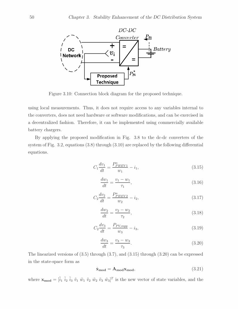
In the second part, the thesis proposes a method for enhancing the stability of the
dc distribution system. Using a nonlinear control strategy, the proposed stability en-
hancement method mitigates the issue of instability by altering the power setpoints of
the battery chargers, bidirectional dc-dc converters, without a need for changing sys-
tem parameters or hardware. The thesis presents mathematical models for the original
and modified systems and demonstrates that the proposed technique expands the stable
operating region of the dc distribution system.
The thesis further proposes an energy management strategy (EMS) for the dc distri-
bution system. Using an on-line constrained optimization algorithm, the proposed EMS
offers two energy exchange options to the PEV owners: (1) The fast energy exchange
option for the owners wishing to minimize the energy exchange time and (2) The optimal
energy exchange option for the owners intend to either minimize their costs of charg-
ing or maximize their revenues through selling their stored energy. The proposed EMS
seamlessly handles all charging/discharging requests from the PEV owners with different
options.
Keywords: Constant-power property, dc distribution system, dc-voltage control,
plug-in electric vehicle, energy management strategy, load management, modeling, opti-
mal charging, smart grid, stability, voltage-sourced converter.
ii
Page 4
To:
my wife, Rokhand, for her generous support,
and the joy of our life, Abtin.
iii
Page 5
Acknowledgement
I would like to express my sincere gratitude to Dr. Amirnaser Yazdani for his excellent
supervision, bright ideas, and continuous encouragement throughout the course of this
research. It has been a great privilege for me to pursue my higher education under his
supervision.
Also, the financial support provided by Dr. Amirnaser Yazdani and Western Univer-
sity is gratefully acknowledged.
iv
Page 7
Contents
Abstract ii
Dedication iii
Acknowledgements iv
List of Figures ix
List of Tables xiii
List of Appendices xiv
List of Abbreviations xv
List of Nomenclature xvi
1 Introduction 1
1.1 Statement of Problem and Thesis Objectives . . . . . . . . . . . . . . . . 1
1.2 Background . . . . . . . . . . . . . . . . . . . . . . . . . . . . . . . . . . 2
1.2.1 Electric Vehicle . . . . . . . . . . . . . . . . . . . . . . . . . . . . 2
1.2.2 Battery Chargers for Electric Vehicles . . . . . . . . . . . . . . . . 3
1.2.3 Power System Integration of Electric Vehicles . . . . . . . . . . . 4
1.3 Thesis Contributions . . . . . . . . . . . . . . . . . . . . . . . . . . . . . 7
1.4 Literature Survey Pertinent to Thesis Contributions . . . . . . . . . . . . 9
2 Modeling of the DC Distribution System 13
2.1 Introduction . . . . . . . . . . . . . . . . . . . . . . . . . . . . . . . . . . 13
2.2 System Configuration and Components . . . . . . . . . . . . . . . . . . . 14
2.2.1 Central VSC . . . . . . . . . . . . . . . . . . . . . . . . . . . . . . 15
Current-Controlled Scheme . . . . . . . . . . . . . . . . . . . . . . 15
vi
Page 8
Controlled dc-Voltage Power Port . . . . . . . . . . . . . . . . . . 18
2.2.2 dc-dc Converters . . . . . . . . . . . . . . . . . . . . . . . . . . . 19
2.3 Mathematical Model . . . . . . . . . . . . . . . . . . . . . . . . . . . . . 21
2.3.1 Existence of a steady state . . . . . . . . . . . . . . . . . . . . . . 23
2.3.2 State-space model . . . . . . . . . . . . . . . . . . . . . . . . . . . 25
2.4 Simulation Results . . . . . . . . . . . . . . . . . . . . . . . . . . . . . . 30
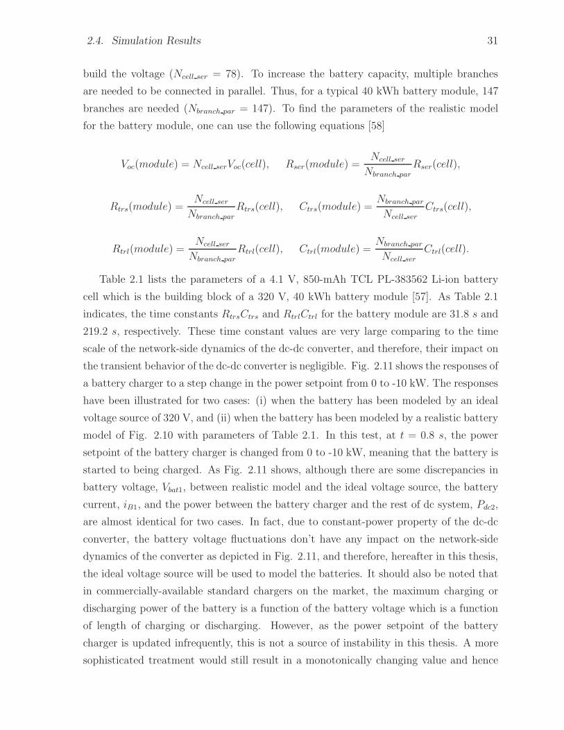
2.4.1 Realistic Battery Model . . . . . . . . . . . . . . . . . . . . . . . 30
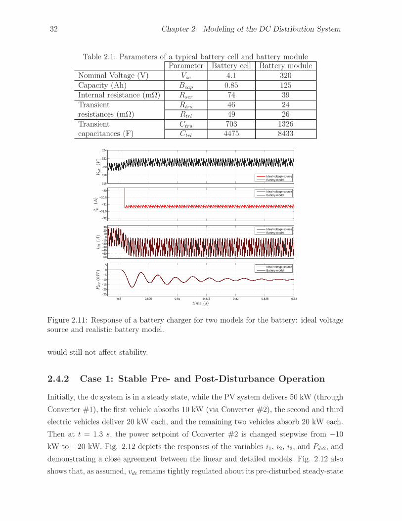
2.4.2 Case 1: Stable Pre- and Post-Disturbance Operation . . . . . . . 32
2.4.3 Case 2: Sensitivity to Cable Length . . . . . . . . . . . . . . . . . 33
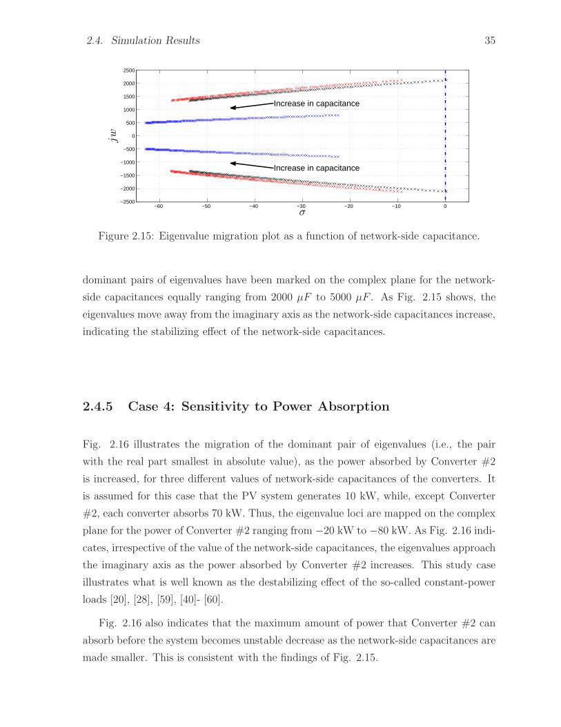
2.4.4 Case 3: Sensitivity to Network-Side Capacitances . . . . . . . . . 34
2.4.5 Case 4: Sensitivity to Power Absorption . . . . . . . . . . . . . . 35
2.4.6 Case 5: Unstable Post-Disturbance Operation . . . . . . . . . . . 36
2.5 dc System with Multiple Nodes of Coupling . . . . . . . . . . . . . . . . 36
2.6 Conclusion . . . . . . . . . . . . . . . . . . . . . . . . . . . . . . . . . . . 39
3 Stability Enhancement of the DC Distribution System 40
3.1 Introduction . . . . . . . . . . . . . . . . . . . . . . . . . . . . . . . . . . 40
3.2 System Configuration . . . . . . . . . . . . . . . . . . . . . . . . . . . . . 41
3.3 Mathematical Model . . . . . . . . . . . . . . . . . . . . . . . . . . . . . 42
3.3.1 Central VSC . . . . . . . . . . . . . . . . . . . . . . . . . . . . . . 42
3.3.2 dc-dc converters . . . . . . . . . . . . . . . . . . . . . . . . . . . . 44
3.4 Stability Enhancement . . . . . . . . . . . . . . . . . . . . . . . . . . . . 47
3.5 Simulation Results . . . . . . . . . . . . . . . . . . . . . . . . . . . . . . 52
3.6 Stability Enhancement for a dc System with Single dc-dc Converter . . . 55
3.7 Stability Enhancement for a dc System with n dc-dc Converters . . . . . 60
3.8 Conclusion . . . . . . . . . . . . . . . . . . . . . . . . . . . . . . . . . . . 64
4 Energy Management Strategy 66
4.1 Introduction . . . . . . . . . . . . . . . . . . . . . . . . . . . . . . . . . . 66
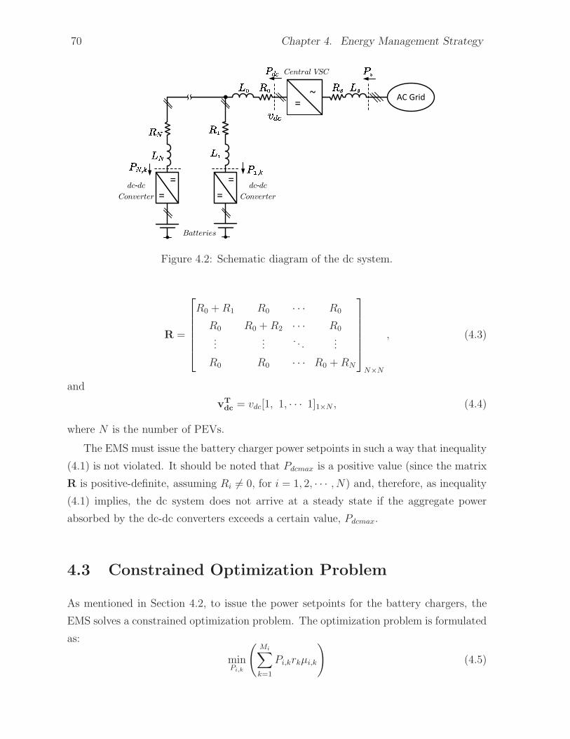
4.2 DC distribution System . . . . . . . . . . . . . . . . . . . . . . . . . . . 67
4.3 Constrained Optimization Problem . . . . . . . . . . . . . . . . . . . . . 70
4.4 Operation of EMS . . . . . . . . . . . . . . . . . . . . . . . . . . . . . . 72
4.5 Determination of Energy Exchange Intervals . . . . . . . . . . . . . . . . 75
4.6 Simulation Results . . . . . . . . . . . . . . . . . . . . . . . . . . . . . . 77
4.6.1 Case I: residential parking lot; evening and night time . . . . . . . 78
vii
Page 9
Scenario I-1 . . . . . . . . . . . . . . . . . . . . . . . . . . . . . . 78
Scenario I-2 . . . . . . . . . . . . . . . . . . . . . . . . . . . . . . 78
Scenario I-3 . . . . . . . . . . . . . . . . . . . . . . . . . . . . . . 79
Scenario I-4 . . . . . . . . . . . . . . . . . . . . . . . . . . . . . . 79
Scenario I-5 . . . . . . . . . . . . . . . . . . . . . . . . . . . . . . 80
4.6.2 Case II: business area parking lot; day time . . . . . . . . . . . . 83
Scenario II-1 . . . . . . . . . . . . . . . . . . . . . . . . . . . . . . 83
Scenario II-2 . . . . . . . . . . . . . . . . . . . . . . . . . . . . . . 84
Scenario II-3 . . . . . . . . . . . . . . . . . . . . . . . . . . . . . . 85
Scenario II-4 . . . . . . . . . . . . . . . . . . . . . . . . . . . . . . 85
4.7 Conclusion . . . . . . . . . . . . . . . . . . . . . . . . . . . . . . . . . . . 87
5 Summary, Conclusions, and Future Work 89
5.1 Summary . . . . . . . . . . . . . . . . . . . . . . . . . . . . . . . . . . . 89
5.2 Conclusions . . . . . . . . . . . . . . . . . . . . . . . . . . . . . . . . . . 90
5.3 Future Work . . . . . . . . . . . . . . . . . . . . . . . . . . . . . . . . . . 91
A Modeling of a droop-based dc-dc converter in a dc system 93
B Positive-Definiteness of R and L matrices 96
C Proof of Equation (2.52) 98
D Study System Parameters for Chapter 2 100
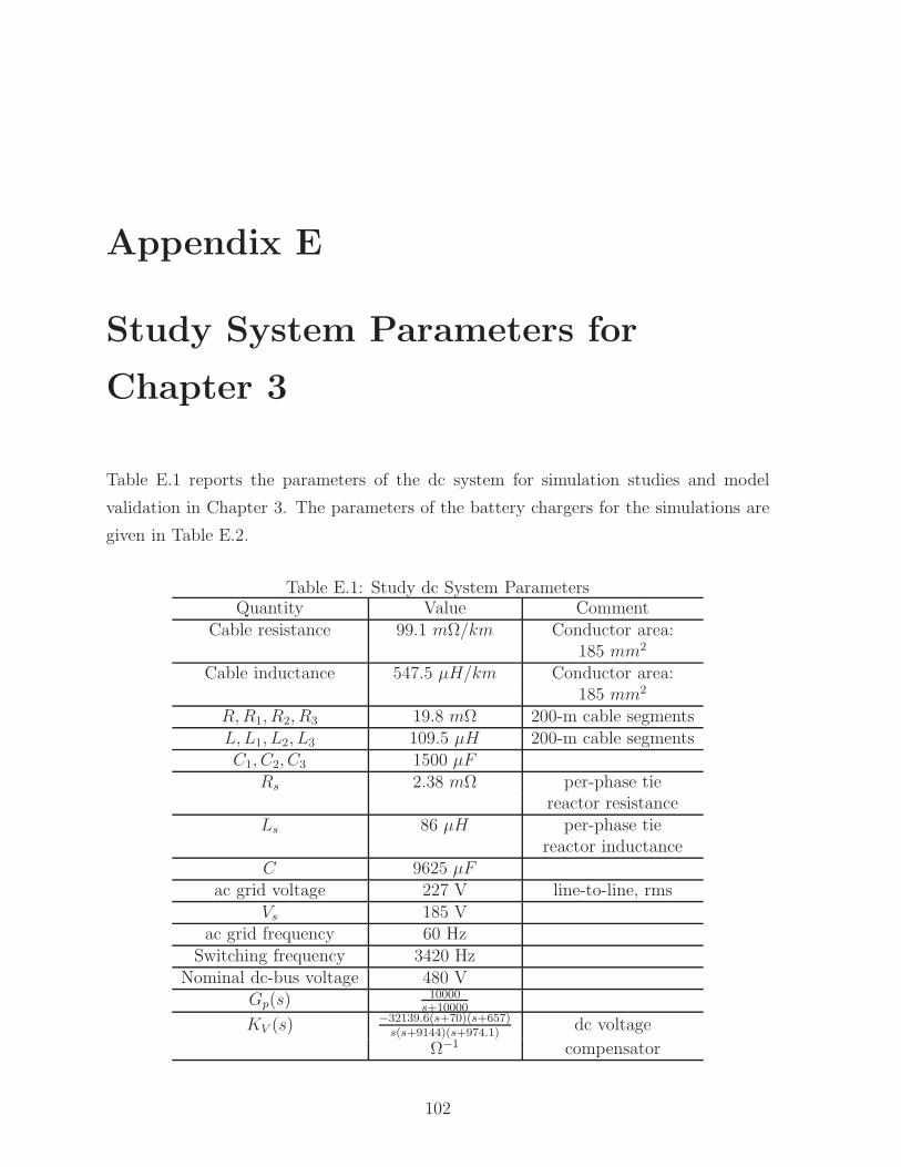
E Study System Parameters for Chapter 3 102
F Study System Parameters for Chapter 4 104
Bibliography 105
Curriculum Vitae 112
viii
Page 10
List of Figures
1.1 The structure of a typical PEV. . . . . . . . . . . . . . . . . . . . . . . . 4
1.2 ac-dc converters for power system integration of electric vehicles. . . . . . 5
1.3 A dc distribution system for power system integration of electric vehicles. 6
2.1 A dc distribution system for power integration of electric vehicles and PV
modules. . . . . . . . . . . . . . . . . . . . . . . . . . . . . . . . . . . . . 15
2.2 Schematic diagram of the dc system. . . . . . . . . . . . . . . . . . . . . 16
2.3 Simplified block diagram of the controlled dc-voltage power port. . . . . 16
2.4 Block diagram of the current-control scheme of the VSC. . . . . . . . . . 17
2.5 Control block diagram of dc-bus voltage controller. . . . . . . . . . . . . 18
2.6 General form of the dc-voltage controller. . . . . . . . . . . . . . . . . . . 20
2.7 The schematic diagram of ith bidirectional dc-dc converter. . . . . . . . . 20
2.8 The simplified model of ith bidirectional dc-dc converter. . . . . . . . . . 21
2.9 Equivalent circuit of the dc system of Fig. 2.2. . . . . . . . . . . . . . . . 22
2.10 Realistic battery model. . . . . . . . . . . . . . . . . . . . . . . . . . . . 30
2.11 Response of a battery charger for two models for the battery: ideal voltage
source and realistic battery model. . . . . . . . . . . . . . . . . . . . . . 32
2.12 Response of the dc-system to a change in Pdc2 from −10 kW to −20 kW
when Pdc1 is 50 kW and Pdc3 to Pdc6 are −20 kW. . . . . . . . . . . . . . 33
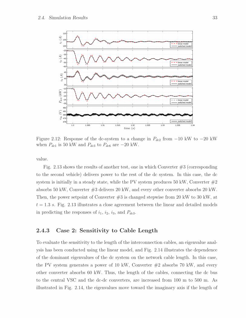
2.13 Response of the dc-system to a change in Pdc3 from 20 kW to 30 kW when
Pdc1 is 50 kW and Pdc2 is −50 kW and Pdc4 to Pdc6 are −20 kW. . . . . . 34
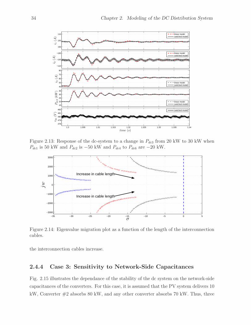
2.14 Eigenvalue migration plot as a function of the length of the interconnection
cables. . . . . . . . . . . . . . . . . . . . . . . . . . . . . . . . . . . . . . 34
2.15 Eigenvalue migration plot as a function of network-side capacitance. . . . 35
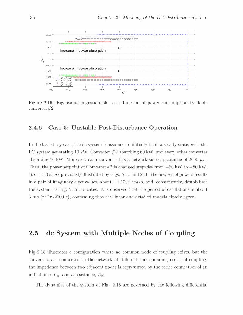
2.16 Eigenvalue migration plot as a function of power consumption by dc-dc
converter#2. . . . . . . . . . . . . . . . . . . . . . . . . . . . . . . . . . . 36
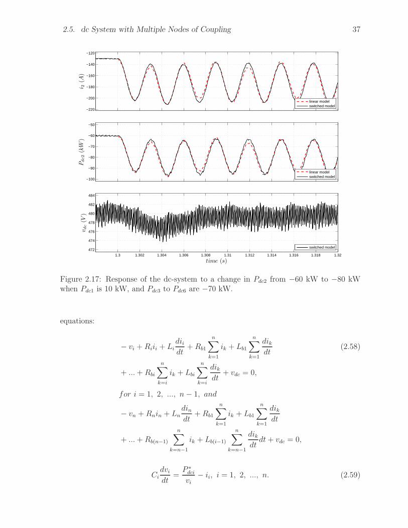
2.17 Response of the dc-system to a change in Pdc2 from −60 kW to −80 kW
when Pdc1 is 10 kW, and Pdc3 to Pdc6 are −70 kW. . . . . . . . . . . . . . 37
ix
Page 11
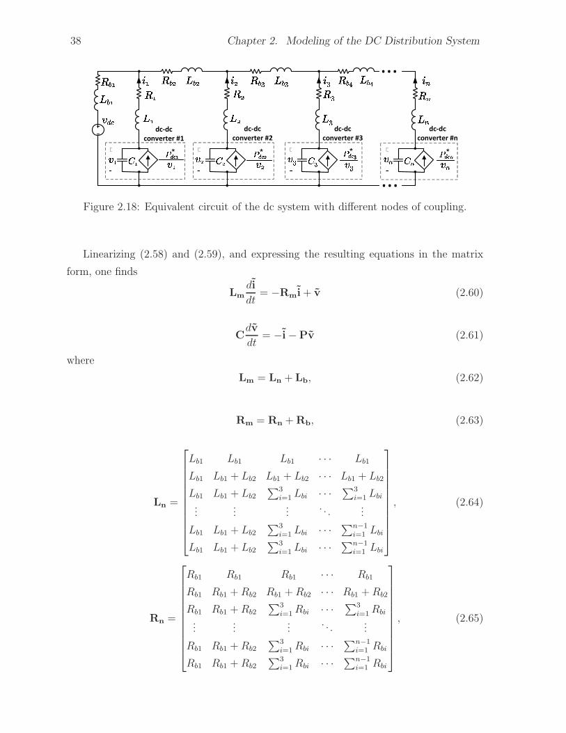
2.18 Equivalent circuit of the dc system with different nodes of coupling. . . . 38
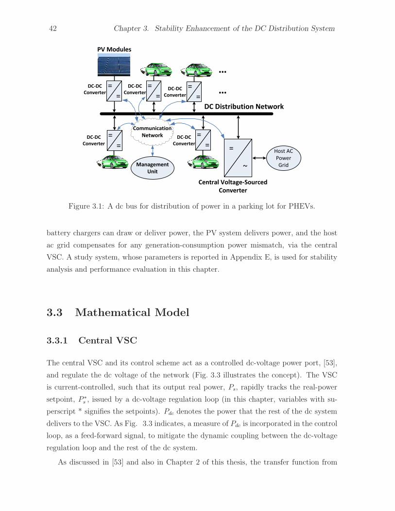
3.1 A dc bus for distribution of power in a parking lot for PHEVs. . . . . . . 42
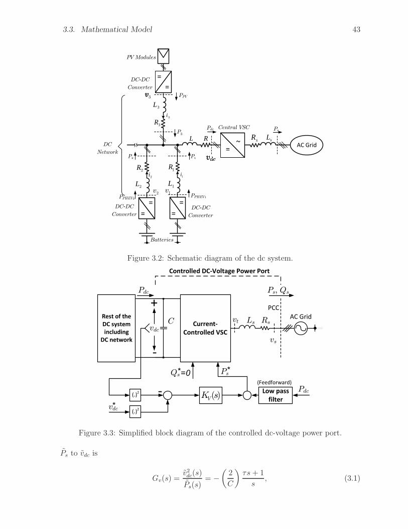
3.2 Schematic diagram of the dc system. . . . . . . . . . . . . . . . . . . . . 43
3.3 Simplified block diagram of the controlled dc-voltage power port. . . . . 43
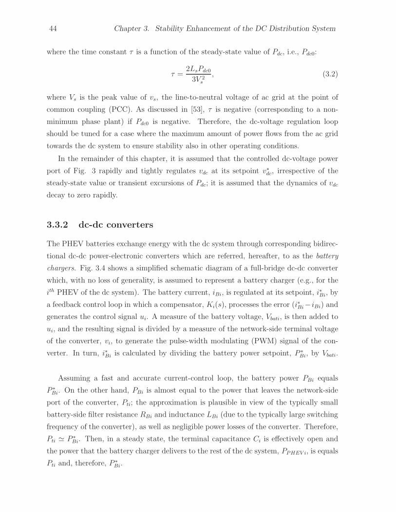
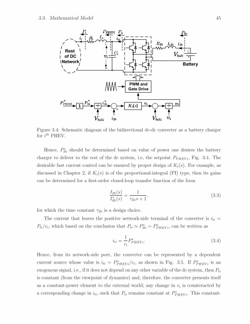
3.4 Schematic diagram of the bidirectional dc-dc converter as a battery charger
for ith PHEV. . . . . . . . . . . . . . . . . . . . . . . . . . . . . . . . . . 45
3.5 Simplified model of the dc-dc converter. . . . . . . . . . . . . . . . . . . . 46
3.6 Equivalent circuit for the analysis of the dc system of Fig. 3.2. . . . . . . 46
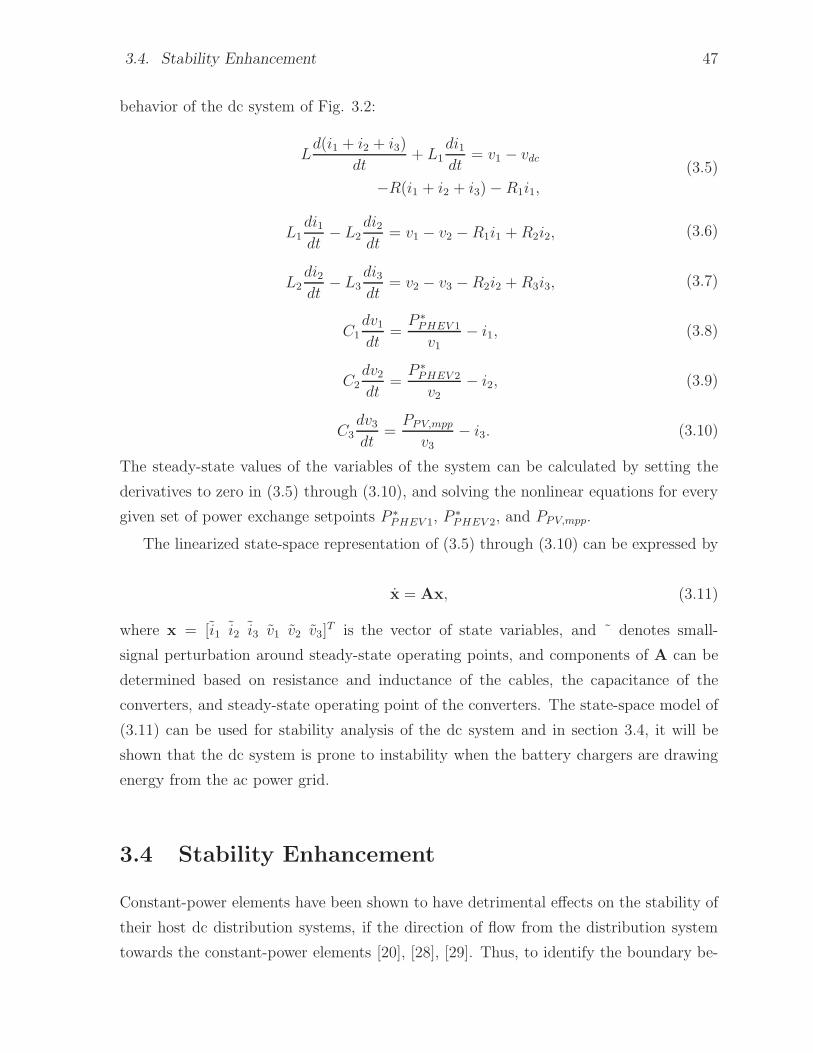
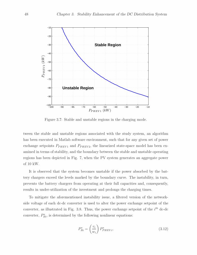
3.7 Stable and unstable regions in the charging mode. . . . . . . . . . . . . . 48
3.8 Modification of the power exchange setpoints of the dc-dc converters. . . 49
3.9 Simplified model of the modified dc-dc converter. . . . . . . . . . . . . . 49
3.10 Connection block diagram for the proposed technique. . . . . . . . . . . . 50
3.11 Boundaries between stable and unstable regions for unmodified and mod-
ified systems with different values of τi. . . . . . . . . . . . . . . . . . . . 52
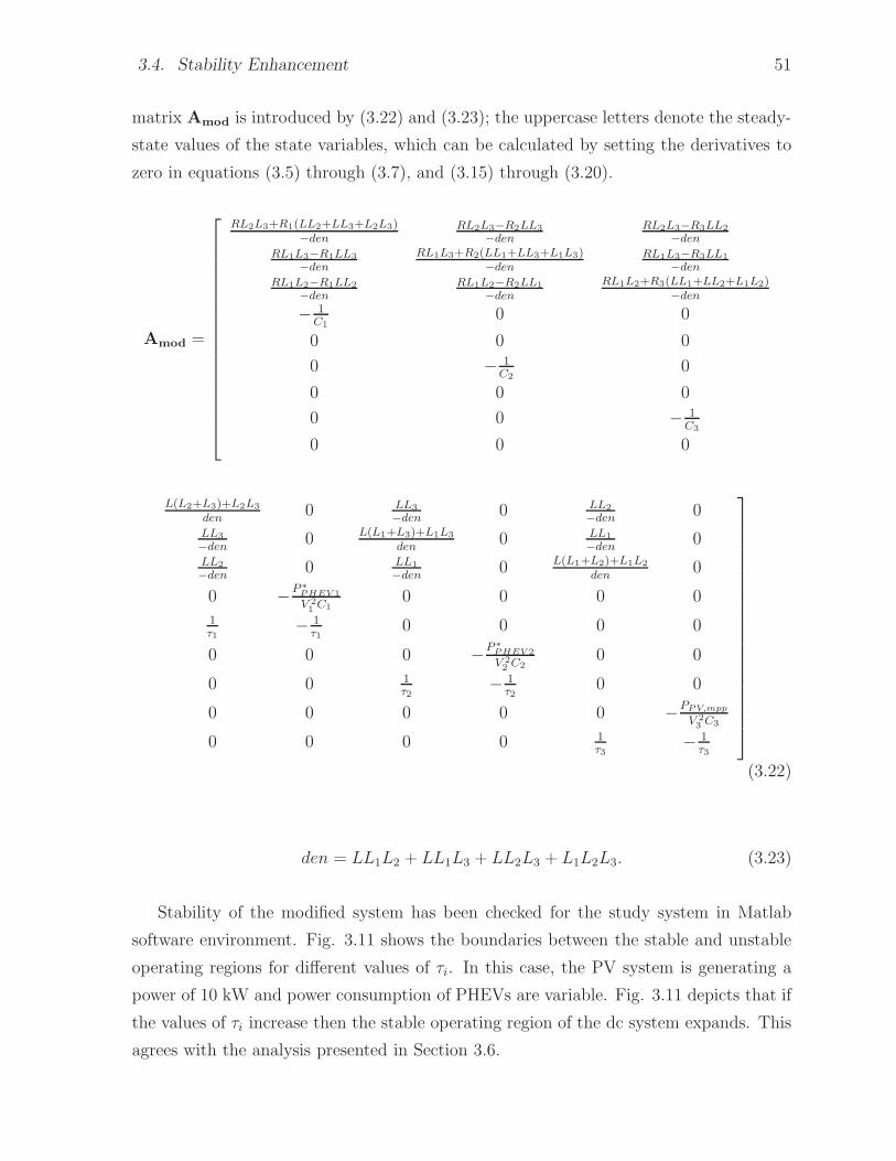
3.12 Boundaries between stable and unstable regions for different values of
power generation of PV modules. . . . . . . . . . . . . . . . . . . . . . . 53
3.13 The dc system response when the power flows from the ac power grid to
the dc system. . . . . . . . . . . . . . . . . . . . . . . . . . . . . . . . . . 54
3.14 The dc system response when the power flows from the dc system to the
ac power grid. . . . . . . . . . . . . . . . . . . . . . . . . . . . . . . . . . 54
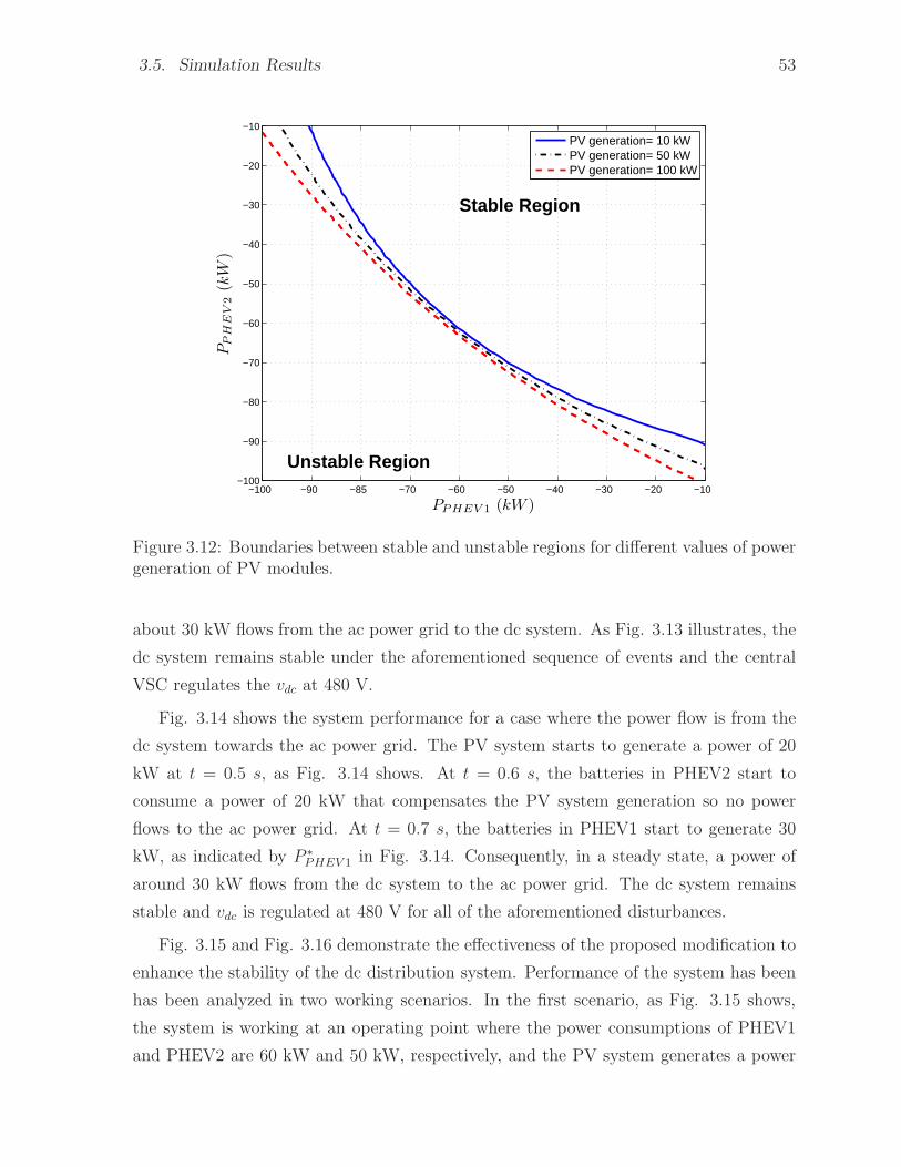
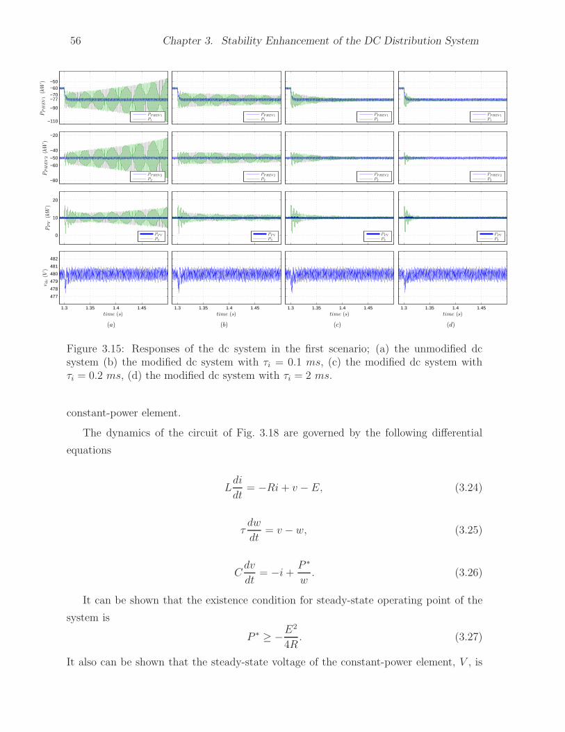
3.15 Responses of the dc system in the first scenario; (a) the unmodified dc
system (b) the modified dc system with τi = 0.1 ms, (c) the modified dc
system with τi = 0.2 ms, (d) the modified dc system with τi = 2 ms. . . 56
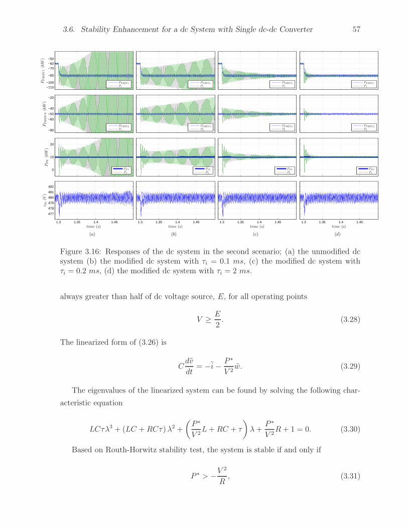
3.16 Responses of the dc system in the second scenario; (a) the unmodified dc
system (b) the modified dc system with τi = 0.1 ms, (c) the modified dc
system with τi = 0.2 ms, (d) the modified dc system with τi = 2 ms. . . 57
3.17 Long-run simulations for vdc; the first unstable scenario for instability
(top), the second unstable scenario for instability (bottom). . . . . . . . . 58
3.18 Proposed modification on a single constant-power element. . . . . . . . . 58
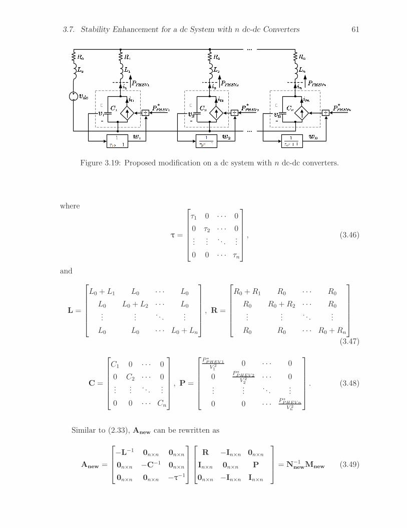
3.19 Proposed modification on a dc system with n dc-dc converters. . . . . . . 61
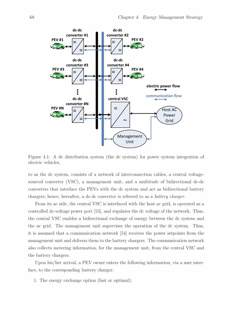
4.1 A dc distribution system (the dc system) for power system integration of
electric vehicles. . . . . . . . . . . . . . . . . . . . . . . . . . . . . . . . . 68
4.2 Schematic diagram of the dc system. . . . . . . . . . . . . . . . . . . . . 70
x
Page 12
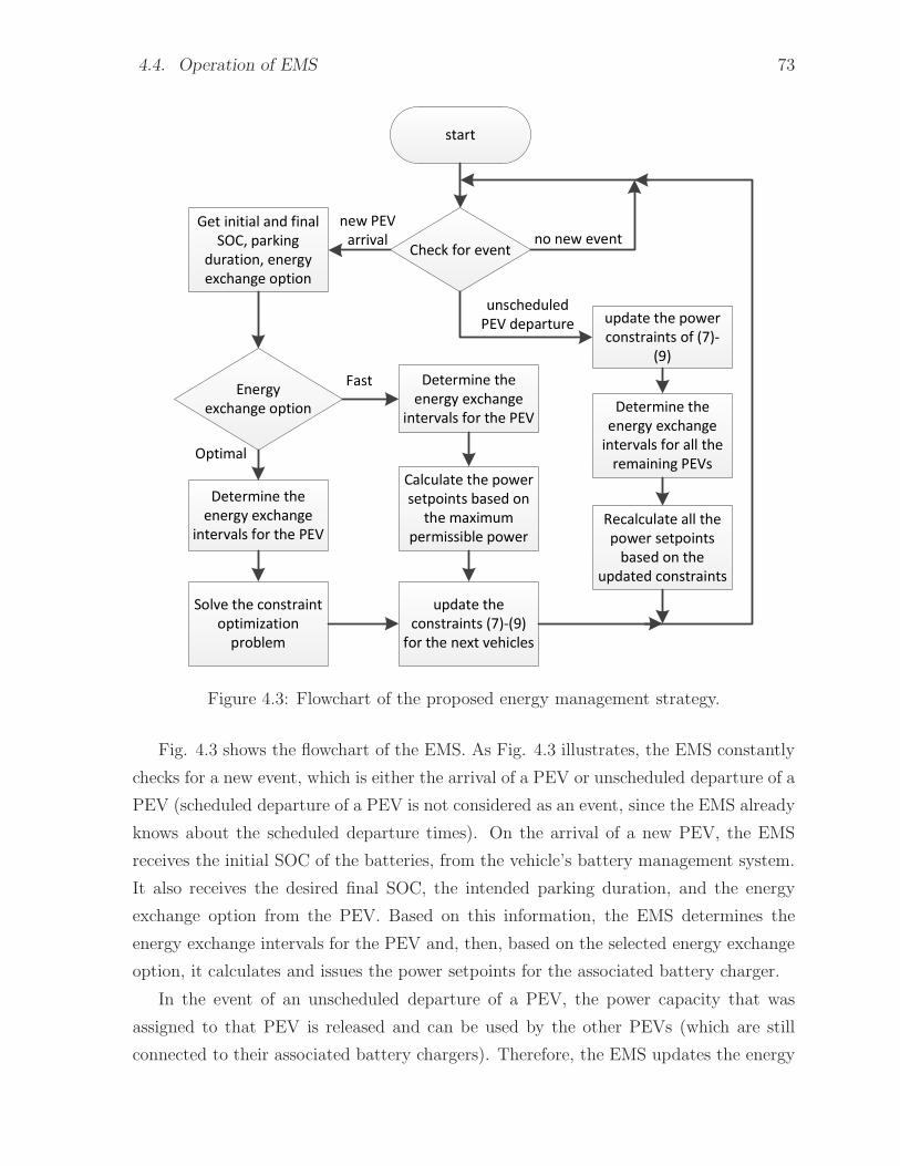
4.3 Flowchart of the proposed energy management strategy. . . . . . . . . . . 73
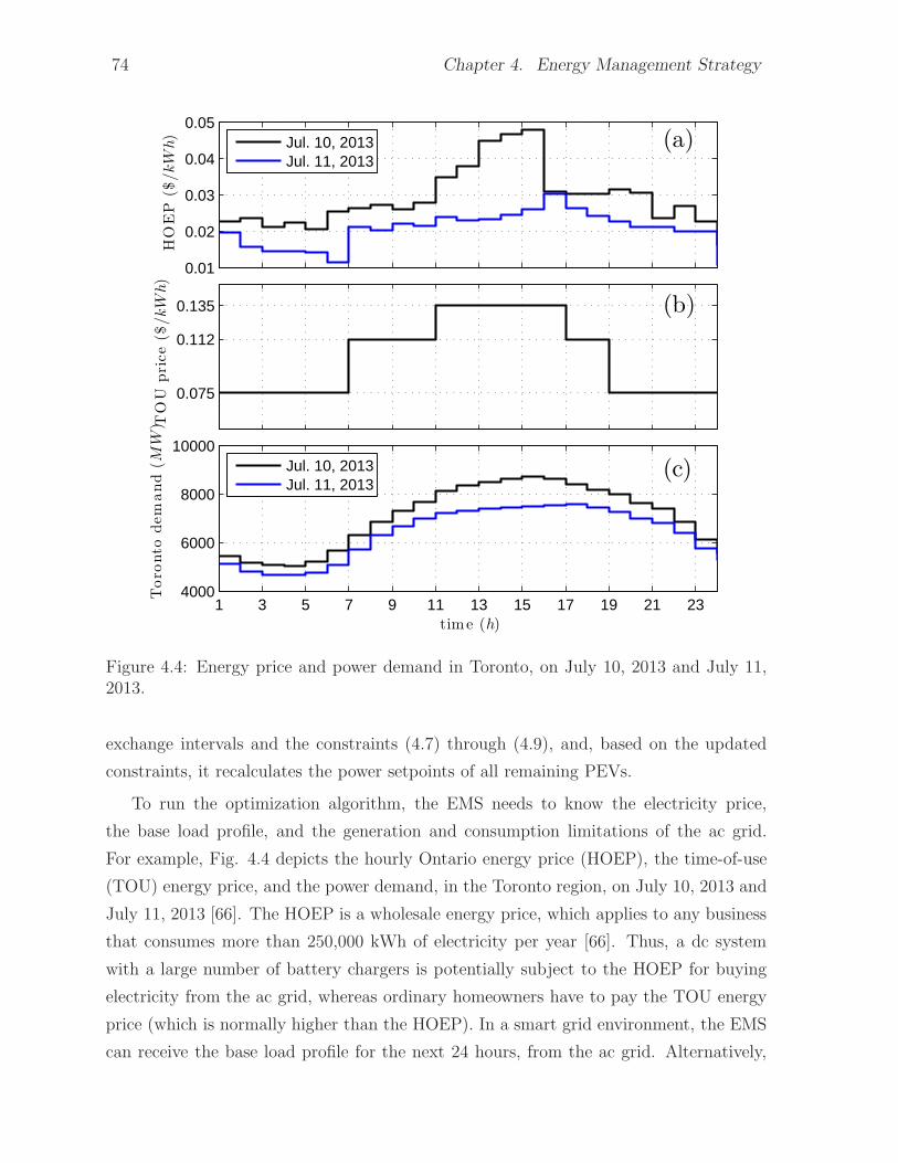
4.4 Energy price and power demand in Toronto, on July 10, 2013 and July 11,
2013. . . . . . . . . . . . . . . . . . . . . . . . . . . . . . . . . . . . . . . 74
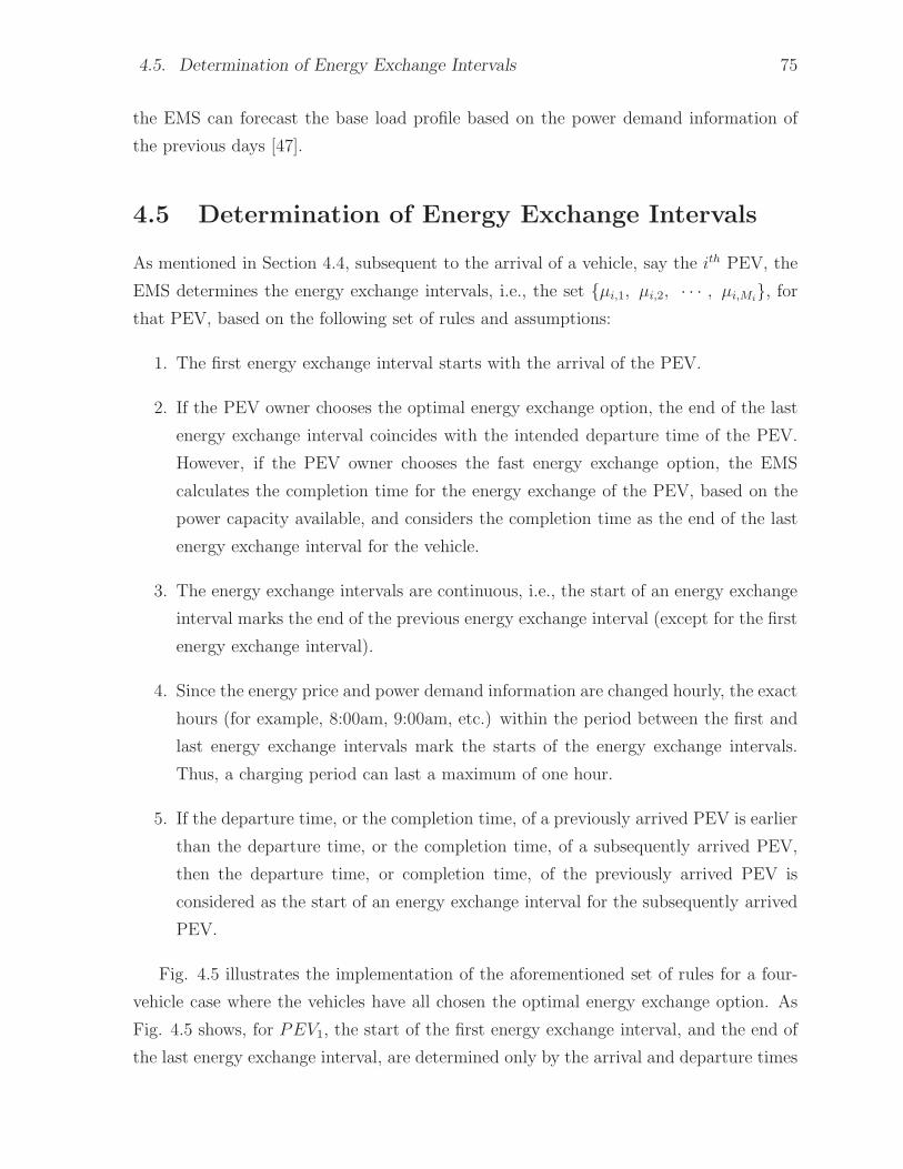
4.5 An example of determination of the energy exchange intervals for four
PEVs with optimal energy exchange option. . . . . . . . . . . . . . . . . 76
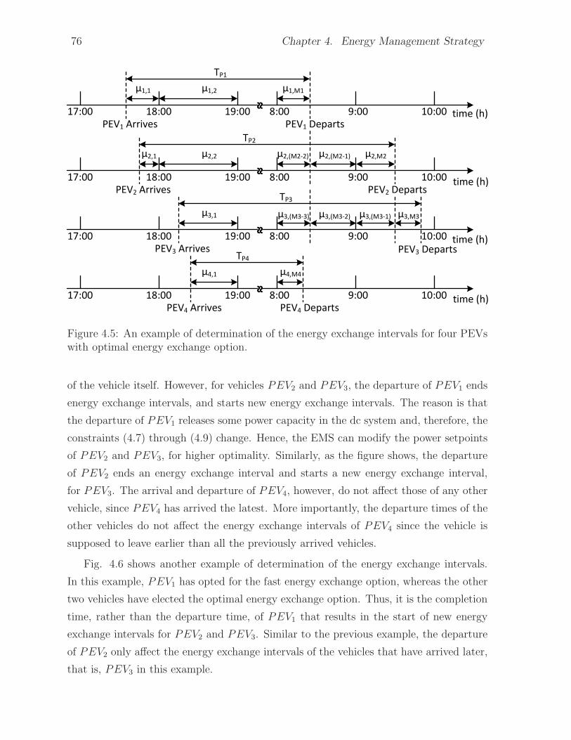
4.6 An example of determination of the energy exchange intervals for three
PEVs; The first PEV with the fast energy exchange option and the other
two PEVs with the optimal energy exchange option. . . . . . . . . . . . . 77
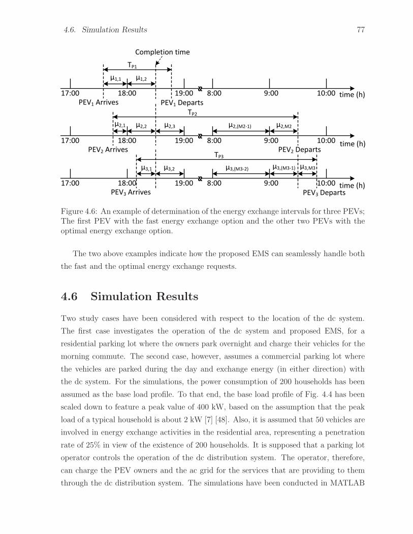
4.7 Case I, Scenario 1: total load under uncoordinated charging of PEVs using
4-kW ac-dc battery chargers. . . . . . . . . . . . . . . . . . . . . . . . . . 78
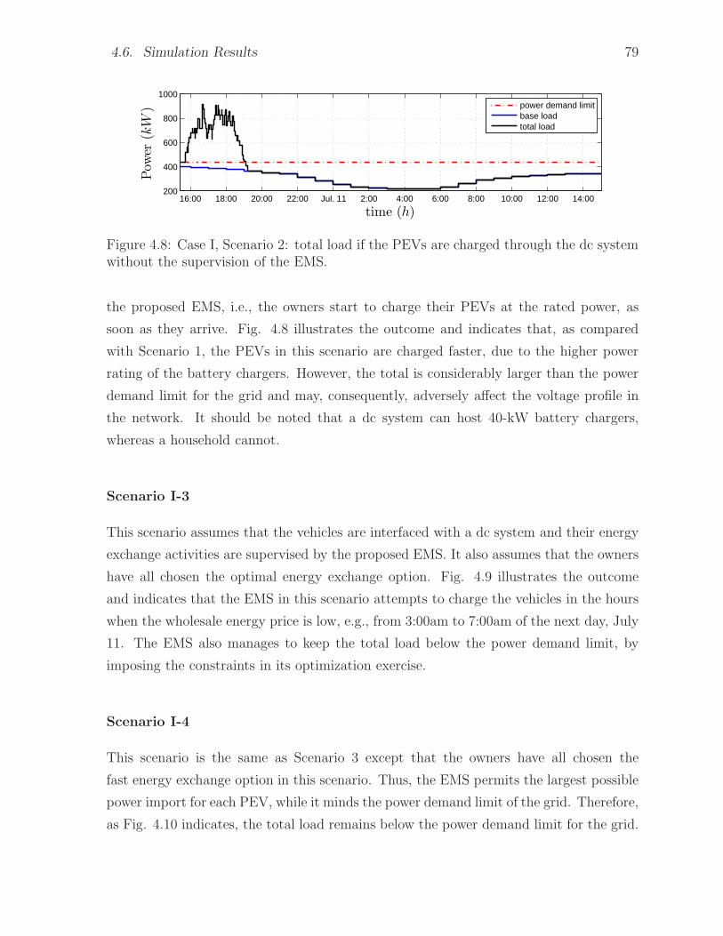
4.8 Case I, Scenario 2: total load if the PEVs are charged through the dc
system without the supervision of the EMS. . . . . . . . . . . . . . . . . 79
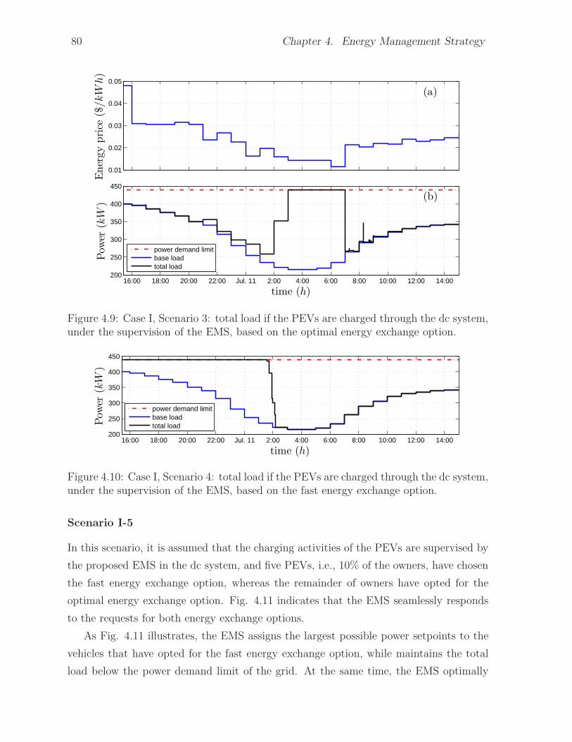
4.9 Case I, Scenario 3: total load if the PEVs are charged through the dc
system, under the supervision of the EMS, based on the optimal energy
exchange option. . . . . . . . . . . . . . . . . . . . . . . . . . . . . . . . 80
4.10 Case I, Scenario 4: total load if the PEVs are charged through the dc sys-
tem, under the supervision of the EMS, based on the fast energy exchange
option. . . . . . . . . . . . . . . . . . . . . . . . . . . . . . . . . . . . . . 80
4.11 Case I, Scenario 5: total load if the PEVs are charged through the dc
system, under the supervision of the EMS, based on a combination of
both fast and optimal energy exchange options. . . . . . . . . . . . . . . 81
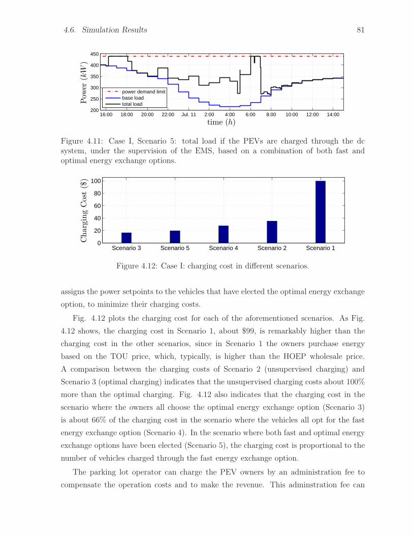
4.12 Case I: charging cost in different scenarios. . . . . . . . . . . . . . . . . . 81
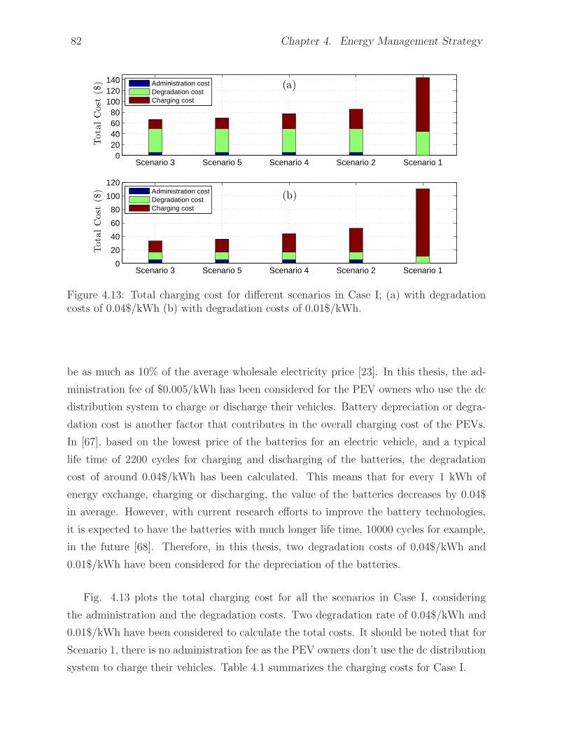
4.13 Total charging cost for different scenarios in Case I; (a) with degradation
costs of 0.04$/kWh (b) with degradation costs of 0.01$/kWh. . . . . . . 82
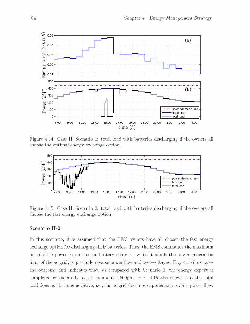
4.14 Case II, Scenario 1: total load with batteries discharging if the owners all
choose the optimal energy exchange option. . . . . . . . . . . . . . . . . 84
4.15 Case II, Scenario 2: total load with batteries discharging if the owners all
choose the fast energy exchange option. . . . . . . . . . . . . . . . . . . . 84
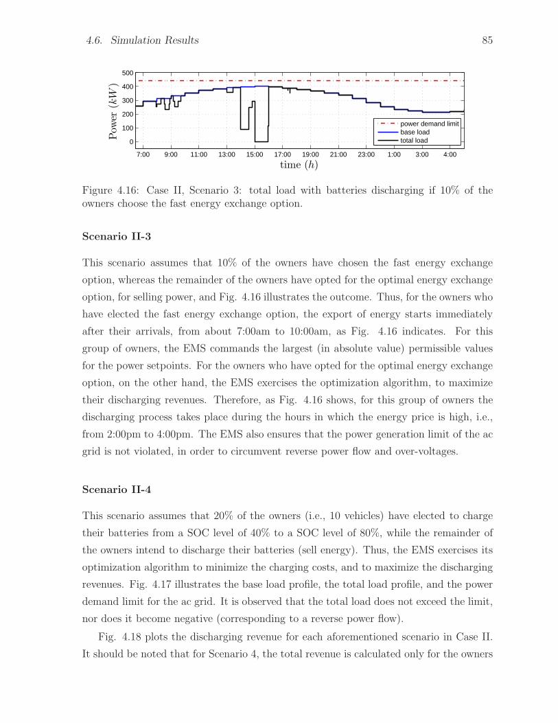
4.16 Case II, Scenario 3: total load with batteries discharging if 10% of the
owners choose the fast energy exchange option. . . . . . . . . . . . . . . 85
4.17 Case II, Scenario 4: total load if 20% of the owners intend to charge their
batteries, while the rest plan to discharge their batteries. . . . . . . . . . 86
4.18 Case II: total discharging revenue in different scenarios. . . . . . . . . . . 86
xi
Page 13
4.19 Revenue and cost for different scenarios in Case II; (a) with degradation
costs of 0.04$/kWh (b) with degradation costs of 0.01$/kWh. . . . . . . 87
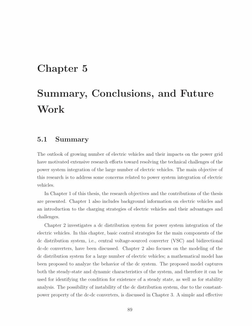
5.1 Equivalent circuit of a dc system with mixed dc-dc converter and linear
loads. . . . . . . . . . . . . . . . . . . . . . . . . . . . . . . . . . . . . . . 92
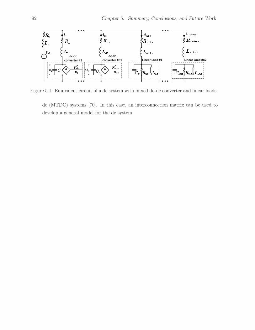
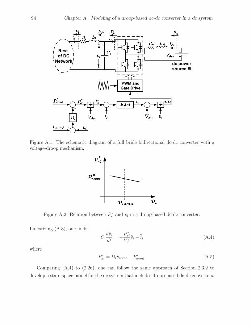
A.1 The schematic diagram of a full bride bidirectional dc-dc converter with a
voltage-droop mechanism. . . . . . . . . . . . . . . . . . . . . . . . . . . 94
A.2 Relation between P ∗si and vi in a droop-based dc-dc converter. . . . . . . 94
A.3 The simplified model of the droop-based dc-dc converter of Fig. A.1. . . 95
xii
Page 14
List of Tables
1.1 Battery capacity and specifications of some electric vehicles on the market 3
1.2 Electric Vehicles Charging Levels . . . . . . . . . . . . . . . . . . . . . . 4
2.1 Parameters of a typical battery cell and battery module . . . . . . . . . . 32
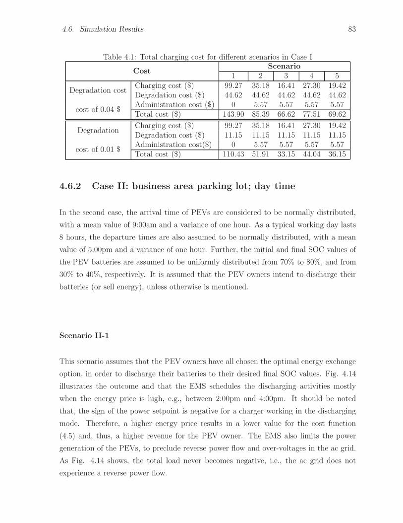
4.1 Total charging cost for different scenarios in Case I . . . . . . . . . . . . 83
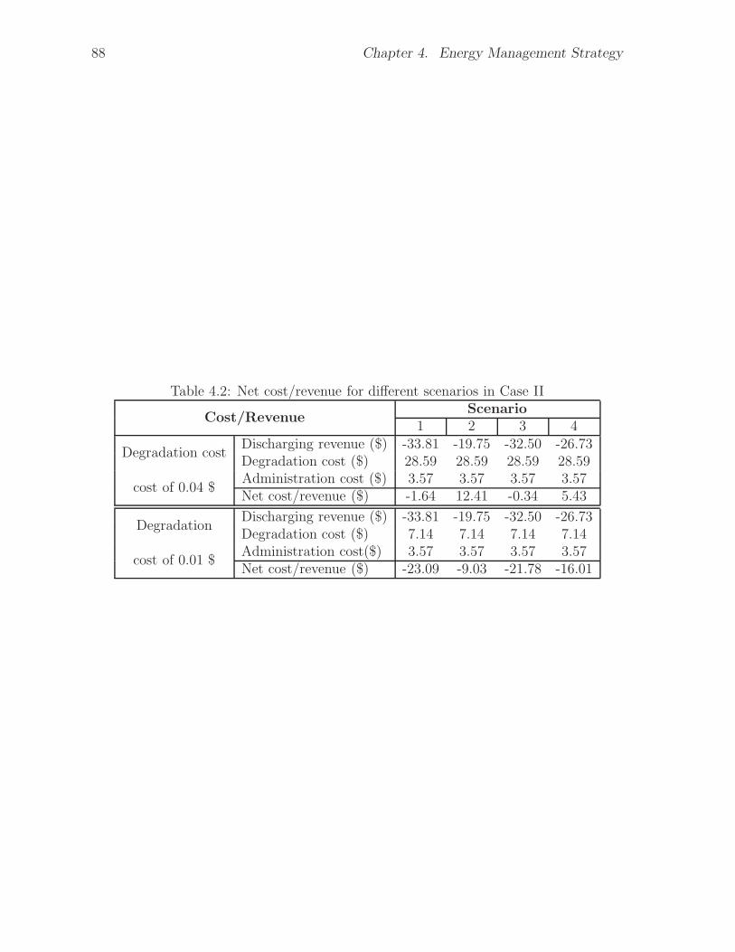
4.2 Net cost/revenue for different scenarios in Case II . . . . . . . . . . . . . 88
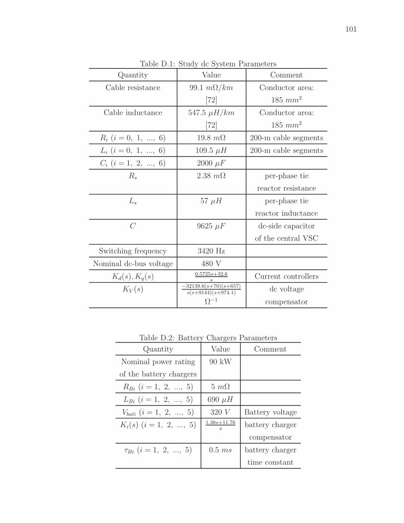
D.1 Study dc System Parameters . . . . . . . . . . . . . . . . . . . . . . . . . 101
D.2 Battery Chargers Parameters . . . . . . . . . . . . . . . . . . . . . . . . 101
E.1 Study dc System Parameters . . . . . . . . . . . . . . . . . . . . . . . . . 102
E.2 Battery Chargers Parameters . . . . . . . . . . . . . . . . . . . . . . . . 103
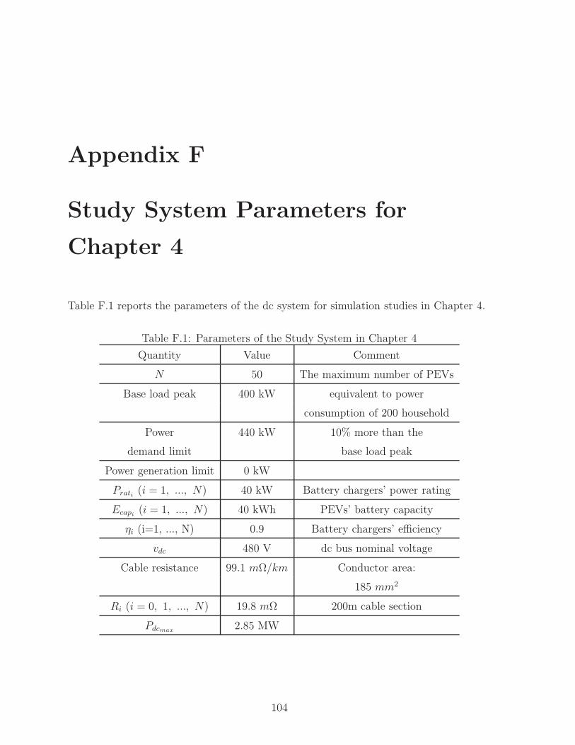
F.1 Parameters of the Study System in Chapter 4 . . . . . . . . . . . . . . . 104
xiii
Page 15
List of Appendices
Appendix A Modeling of a droop-based dc-dc converter in a dc system . . . . . . 93
Appendix B Positive-Definiteness of R and L matrices . . . . . . . . . . . . . . . 96
Appendix C Proof of Equation (2.52) . . . . . . . . . . . . . . . . . . . . . . . . . 98
Appendix D Study System Parameters for Chapter 2 . . . . . . . . . . . . . . . . 100
Appendix E Study System Parameters for Chapter 3 . . . . . . . . . . . . . . . . 102
Appendix F Study System Parameters for Chapter 4 . . . . . . . . . . . . . . . . 104
xiv
Page 16
Abbreviations and Symbols
ac Alternating Current
dc Direct Current
BEV Battery Electric Vehicle
EMS Energy Management Strategy
EV Electric Vehicle
EVSE Electric Vehicle Supply Equipment
HOEP Hourly Ontario Energy Price
ICE Internal Combustion Engine
MPPT Maximum Power-Point Tracking
PCC Point of Common Coupling
PEV Plug-in Electric Vehicle
PFC Power-Factor Correction
PHEV Plug-in Hybrid Electric Vehicle
PI Proportional-Integral
PLL Phase-Locked Loop
PSCAD Power System Computer-Aided Design
PV Photo-Voltaic
PWM Pulse-Width Modulation
SAE Society of Automotive Engineers
TOU Time-of-Use
SOC State-of-Charge
VSC Voltage-Sourced Converter
xv
Page 17
Nomenclature
Ps Real power at PCC
Qs Reactive power at PCC
Ls Linking inductance
Rs Parasitic resistance of Ls (including on-state resistance of the VSC switches)
Pdc Total power at dc terminal of the VSC
C dc-side capacitance of the VSC
vdc dc bus voltage
Pdci Power that flows to the network terminal of ithdc-dc converter
vi Voltage of the network terminal of ith dc-dc converter
Ri Cable resistance of the dc network branches
Li Cable inductance of the dc network branches
Vs Peak value of the ac grid line-to-neutral
ω Power system frequency
Vbati Voltage of ith battery
PBi Power of ith battery
ii Current of the network-side terminal of ith dc-dc converter
Ci Capacitance of the network-side terminal of ith dc-dc converter
PPV Power of PV modules
PdcmaxMaximum permissable power that can be imported by the dc system
Prati Power rating of ith battery charger
ηi Efficiency of ith battery charger
µi,k Duration of kth energy exchange interval for ith PEV
rk Energy price in kth energy exchange interval
Ei Exchangeable energy of ith PEV
SOCi,i Initial value for State-of-Charge of ith PEV
SOCi,f Final value for State-of-Charge of ith PEV
TPiParking duration of ith PEV
Ecapi Battery capacity of ith PEV
xvi
Page 18
Chapter 1
Introduction
1.1 Statement of Problem and Thesis Objectives
The power system integration of Plug-in Electric Vehicles (PEVs) and the possibility of
bidirectional power exchange between them and the host grid have attracted attentions
recently [1,2]. In addition to providing traction power, batteries in a PEV can potentially
be used for bulk energy storage in such applications as peak shaving, reactive power
compensation [3], and the integration of renewable energy resources. Public parking
areas within hospitals, department stores, and residential and commercial premises are
examples of locations where a large number of PEVs can be integrated with the power
system. Thus, PEV owners can charge their batteries (or buy energy from the rest of the
system) or discharge them (or sell energy to the rest of the system) based on their trip
plans, cost of electricity, and the State of Charge (SOC) of the batteries; electric energy
can be stored at night when the cost of electricity is low, and then sold at a higher price
if there is a high demand for electricity or if the host grid is in need of ancillary services.
This can be achieved through bidirectional power-electronic converters [4, 5].
The increasing number of PEVs is, however, expected to adversely impact the power
system [6]. Charging a large number of PEVs at the same time in the evening, when the
owners come back home from work and connect their vehicles to the battery chargers,
could significantly stress the power grid; causing voltage fluctuations, suboptimal gener-
ation dispatch, degraded system efficiency, and increasing the likelihood of blackouts due
to network overloads [7]. Therefore, suitable infrastructure and smart charging strategies
are required to circumvent or mitigate these potentially negative impacts.
This thesis concentrates on bidirectional power exchange between a large number of
1
Page 19
2 Chapter 1. Introduction
plug-in electric vehicles and the ac power grid. Hereinafter, Plug-in Electric Vehicles
(PEVs) and Plug-in Hybrid Electric Vehicles (PHEVs) will be used interchangeably to
represent all electric vehicles.
The objectives of the thesis are:
• To introduce a dc distribution system for the integration of a large number of
electric vehicles, including PEVs and PHEVs, into the ac power grid, in public
parking areas.
• To develop a mathematical model for the dc distribution system to capture both
the steady-state and dynamic characteristics of the system, to analyze the stability
of the system, and to check for the existence of the steady-state operating point of
the system.
• To develop a control strategy to mitigate the instability problem of the dc distribu-
tion system and expand the stable operation region of the system, without a need
for changing system parameters or hardware.
• To develop an energy management strategy for the dc distribution system to enable
an optimal energy exchange among the PEV battery chargers in the dc system and
the ac power grid.
1.2 Background
1.2.1 Electric Vehicle
Electric vehicles can be generally categorized in three different groups:
• Plug-in Electric Vehicle (PEV)
In this category, the electric vehicles are only powered by the on-board battery
and there are no internal combustion engines in the vehicles. The batteries can be
charged from a power source outside of the electric vehicles, through a connector.
In the literature, battery electric vehicles (BEVs) are also used to refer to these
electric vehicles.
• Plug-in Hybrid Electric Vehicle (PHEV)
Electric vehicles in this category have both electric motors and internal combustion
engines (ICEs). The batteries can be charged from a power source outside of the
Page 20
1.2. Background 3
Table 1.1: Battery capacity and specifications of some electric vehicles on the market
Model TypeBattery
TechnologyBatteryCapacity
All-ElectricRange
ChevroletVolt
PHEV Li-Ion 17.1 kWh 61 km
Mitsubishii-MiEV
PEV Li-Ion 16 kWh 96 km
FordFusion SE Energi
PHEV Li-Ion 7.6 kWh 30 km
NissanLeaf
PEV Li-Ion 24 kWh 159 km
ToyotaPrius
PHEV Li-Ion 4.4 kWh 22 km
TeslaModel S
PEV Li-Ion 85 kWh 480 km
electric vehicles. Therefore, these electric vehicles can exchange power with the
host power grid. PHEVs typically operate in a “blended” mode, using the ICE
and electric motor together, to substantially reduce gasoline consumption when
operating in battery charge depletion mode.
• Hybrid Electric Vehicle (HEV)
In this category, the vehicles have both electric motors and internal combustion
engines. However, the batteries cannot be charged from a power source outside of
the vehicle.
In this thesis, only the first two categories, i.e., PEV and PHEV, are considered for
study, as the electric vehicles in the third category do not exchange power with the host
power grid. Table 1.1 lists the type and battery capacity of some electric vehicles on the
market [8–13].
1.2.2 Battery Chargers for Electric Vehicles
Battery chargers for electric vehicles have been classified in three different levels by the
Society of Automotive Engineers (SAE). Table 1.2 summarizes the charging levels for
PEVs based on SAE J-1772 standard [14, 15]. Level 1 is the slow charging level where
the electric vehicles can be plugged in to a convenience ac power outlet and the maximum
charging power level is 1.92 kW. At this level, the battery charger is usually inside the
vehicle. For Level 2 charging, the maximum power is 19.2 kW and it uses 240 Vac
power outlet. Level 3 offers commercially fast battery charging for electric vehicles and it
typically operates with 480 V or higher three phase circuit, requiring an off-board charger.
Page 21
4 Chapter 1. Introduction
Table 1.2: Electric Vehicles Charging Levels
Power Level Charger Typical Energy Supply Expected Charging VehicleTypes Location Use Interface Power Level Time TechnologyLevel 1
120 Vac (US)230 Vac (EU)
On-board1-phase
Charging athome or office
Convenienceoutlet
1.4kW (12A)1.9kW (20A)
4-11 hours11-36 hours
PHEVs (5-15kWh)EVs (16-50kWh)
Level 2240 Vac (US)400 Vac (EU)
On-board1- or 3-phase
Charging atprivate or
public outlets
DedicatedEVSE
4kW (17A)8kW (32A)
19.2kW (80A)
1-4 hours2-6 hours2-3 hours
PHEVs (5-15kWh)EVs (16-30kWh)EVs (3-50kWh)
Level 3208-600
Vac or Vdc
Off-board3-phase
Commercial,analogous to afilling station
DedicatedEVSE
50kW100kW
0.4-1 hour0.2-0.5 hour
EVs (20-50kWh)
Figure 1.1: The structure of a typical PEV.
Fig. 1.1 shows the internal structure of a typical electric vehicle and the battery chargers
at different levels [15]. The SAE J1772 standard prescribes that Level 1 and Level 2
battery chargers should be located on the electric vehicle. For Level 3, the standard
considers off-board battery charger. In this case, the battery charger can be directly
connected to the battery of the electric vehicle. This enables Level 3 battery chargers to
perform fast charging in public places such as parking lots on commercial premises.
1.2.3 Power System Integration of Electric Vehicles
In most proposed strategies for power system integration of electric vehicles, ac-dc power-
electronic converters act as the battery chargers and are directly interfaced with the
power grid [15, 16], as is shown in Fig. 1.2. Alternatively, dc distribution networks
embedding dc-dc converters (as the battery chargers) have been proposed for power
system integration of electric vehicles in public parking areas, where a sizeable number
Page 22
1.2. Background 5
electric power flow communication flow
~
=
PFC
ac-dc converter #1
Host AC
Power
Grid
EV
~
=
PFC
ac-dc converter #3
EV
~
=
PFC
ac-dc converter #n-1
…
EV
~
=
PFC
ac-dc converter #2
EV
~
=
PFC
ac-dc converter #4
EV
~
=
PFC
ac-dc converter #n
…
PV Modules
Figure 1.2: ac-dc converters for power system integration of electric vehicles.
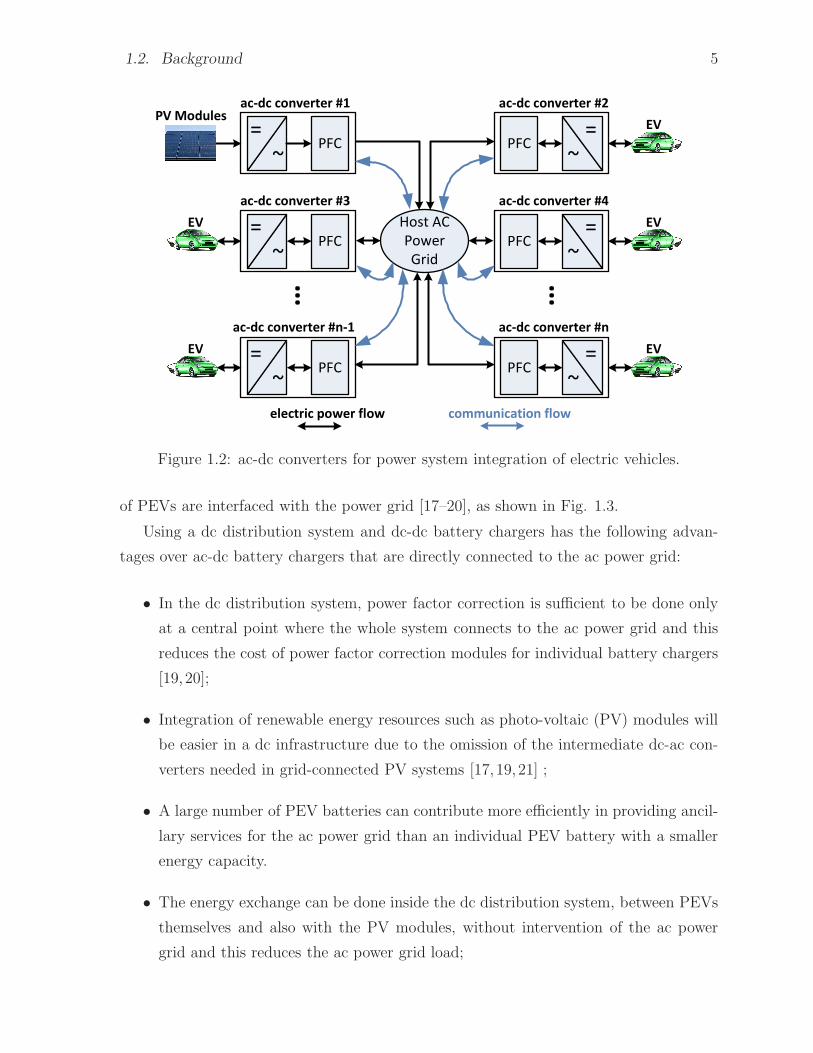
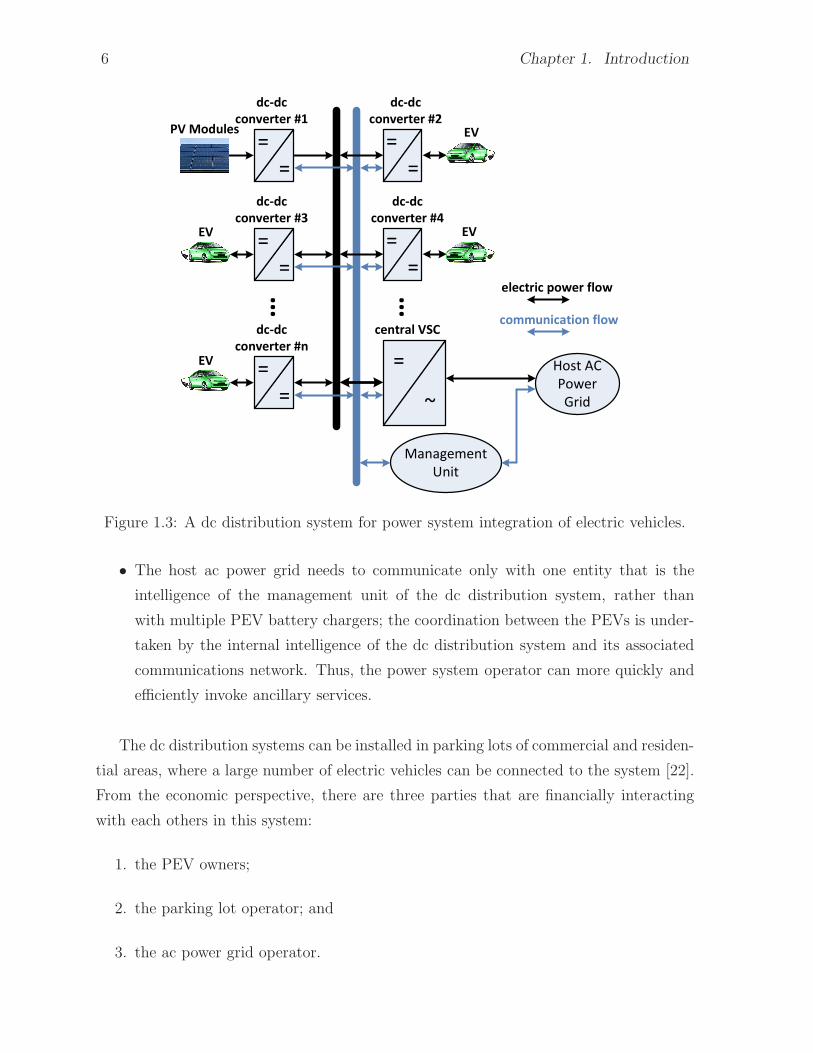
of PEVs are interfaced with the power grid [17–20], as shown in Fig. 1.3.
Using a dc distribution system and dc-dc battery chargers has the following advan-
tages over ac-dc battery chargers that are directly connected to the ac power grid:
• In the dc distribution system, power factor correction is sufficient to be done only
at a central point where the whole system connects to the ac power grid and this
reduces the cost of power factor correction modules for individual battery chargers
[19, 20];
• Integration of renewable energy resources such as photo-voltaic (PV) modules will
be easier in a dc infrastructure due to the omission of the intermediate dc-ac con-
verters needed in grid-connected PV systems [17, 19, 21] ;
• A large number of PEV batteries can contribute more efficiently in providing ancil-
lary services for the ac power grid than an individual PEV battery with a smaller
energy capacity.
• The energy exchange can be done inside the dc distribution system, between PEVs
themselves and also with the PV modules, without intervention of the ac power
grid and this reduces the ac power grid load;
Page 23
6 Chapter 1. Introduction
=
= =
=
dc-dc
converter #1
dc-dc
converter #2
=
= =
=
dc-dc
converter #3
dc-dc
converter #4
=
=
dc-dc
converter #n
central VSC
… …
Host AC
Power
Grid
PV Modules
Management
Unit
electric power flow
communication flow
=
~
EV EV
EV
EV
Figure 1.3: A dc distribution system for power system integration of electric vehicles.
• The host ac power grid needs to communicate only with one entity that is the
intelligence of the management unit of the dc distribution system, rather than
with multiple PEV battery chargers; the coordination between the PEVs is under-
taken by the internal intelligence of the dc distribution system and its associated
communications network. Thus, the power system operator can more quickly and
efficiently invoke ancillary services.
The dc distribution systems can be installed in parking lots of commercial and residen-
tial areas, where a large number of electric vehicles can be connected to the system [22].
From the economic perspective, there are three parties that are financially interacting
with each others in this system:
1. the PEV owners;
2. the parking lot operator; and
3. the ac power grid operator.
Page 24
1.3. Thesis Contributions 7
In a dc distribution system, the PEV owners can use the wholesale energy price to
charge their vehicles. The wholesale energy price is usually much cheaper than the retail
energy price, even considering the administration fee from the parking lot operator, and
therefore, the PEV owners will financially gain when they use the dc distribution system
to connect their vehicles to the ac power grid. Moreover, by using a smart charging
strategy, the charging activities can be shifted to the time frames when the energy price
is even cheaper, hence further reduce the cost of the battery charging.
The parking lot operator can make revenue by:
• charging the PEV owners an adminstration fee for charging or discharging energy
(per kWh) [23, 24]; and
• charging the ac power grid for providing the ancillary services.
The ac power grid benefits from the dc system by using the ancillary services which
are provided. Using the battery capacity of a large number of PEVs, the dc distribution
system has the capacity to provide a variety of services to the ac power grid such as peak
shaving, load shaping, frequency regulation, ac voltage support, and power regulation
service [25]. By using peak shaving service, for example, the ac power grid avoids the
installation of capacity only to supply the peaks of a highly variable loads. To provide
this service, the dc distribution system supply energy to the high-demand customers of
the ac power grid at the peak-time.
One of the problems with dc distribution systems is the possibility of instability in
the system. Due to the constant-power property of dc-dc converters, the dc system
becomes unstable if the powers absorbed by the converters exceed certain values [20].
This phenomenon inflicts a limit on the maximum power that can be imported to charge
the batteries and, consequently, precludes full utilization of the installed capacities and
prolongs the charging times. Therefore, it is imperative to devise a stability enhancement
technique in order to push the limits and expand the stable operating region of the dc
distribution system.
1.3 Thesis Contributions
The main contributions of this thesis can be listed as follows:
• The thesis proposes a dc distribution system for power system integration of plug-
in electric vehicles. The proposed system is expected to be more efficient and
Page 25
8 Chapter 1. Introduction
economical than an equivalent aggregate of ac-dc battery charges connected to the
ac grid, since it relieves the battery chargers from the need for a bidirectional,
front-end, power-factor correction (PFC) stage. Further, due to its DC nature, the
proposed system is amenable to integration of Photovoltaic (PV) modules. The
thesis also proposes a systematic method for developing a model of a dc distribution
system, based on the configuration of the system. The developed model is of the
matrix form and, therefore, can readily be expanded to represent a system of any
desired number of dc-dc converters. The model captures both the steady-state and
dynamic characteristics of the system, and includes port capacitors of the converters
and the interconnection cables. Thus, it can be used for identifying the condition
for existence of a steady state, as well as for stability analysis.
• The thesis further proposes a method for enhancing the stability of a dc distribution
system that integrates plug-in electric vehicles with the ac power grid. Using a
nonlinear control strategy, the proposed stability enhancement method mitigates
the issue of instability by altering the power setpoints of the battery chargers,
bidirectional dc-dc converters, without a need for changing system parameters or
hardware. The thesis further presents mathematical models for the original and
modified systems and demonstrates that the proposed technique expands the stable
operating region of the dc distribution system.
• Finally, the thesis proposes an energy management strategy (EMS) for the dc dis-
tribution system for power system integration of plug-in electric vehicles (PEVs).
Using an on-line constrained optimization algorithm, the proposed EMS manages
the power flow within the dc system. Thus, the PEV owners can charge or dis-
charge their batteries, based on the state-of-charge (SOC) of the batteries and
their upcoming trip plans. The EMS offers two energy exchange options to the
PEV owners: (i) The fast energy exchange option for the owners wishing to min-
imize the energy exchange time and (ii) The optimal energy exchange option for
the owners intend to either minimize their costs of charging or maximize their rev-
enues through selling their stored energy. The proposed EMS seamlessly handles
all charging/discharging requests from the PEV owners with different options and,
at the same time, it takes into account the power demand and power generation
limits of the ac grid, to preclude under-voltage, over-voltage, and reverse power
flow issues.
Page 26
1.4. Literature Survey Pertinent to Thesis Contributions 9
1.4 Literature Survey Pertinent to Thesis Contribu-
tions
Chapter 2 of this thesis focuses on the mathematical model for the dc distribution sys-
tem. A dc distribution system is expected to offer a higher efficiency and to enable an
easier integration of renewable energy sources such as photovoltaic (PV) and fuel-cell sys-
tems [26,27], as compared with a system of ac-dc battery chargers. However, it is prone
to instabilities due to constant-power property of the hosted dc-dc converters, if powers
drawn by the dc-dc converters (to charge the batteries) exceed certain limits [20,28,29].
Thus, one needs a model of the system to characterize the steady-state and dynamic be-
haviors of the system. Such a model should be tractable, while adequately accurate, and
it should also represent both the steady-state and dynamic characteristics of the system.
One should also be able to systematically expand it to represent a system of any desired,
and most likely large, number of dc-dc converters. To the author’s best of knowledge, the
published technical literature does not present a model with the aforementioned features.
Several prior studies have reported system-level models for dc distribution systems
[30–33]. The main issue associated with the aforementioned studies is that they consider
a limited number of dc-dc converters on the dc distribution system and develop the
model for the system based on that assumption. Reference [30], proposes a model for a dc
distribution system, but the model only describes the steady-state behavior of the system.
Reference [31] develops a model, and proposes a method for stabilizing a dc distribution
system. However, the presented model is limited to three converters and, consequently,
cannot be adopted for a dc distribution system with a large number of converters. In [27]
a model is proposed for a dc distribution system with multiple loads and sources, but
it does not consider the interconnection cables of the system. Reference [34] proposes a
reduced-order model for a generic dc microgrid. The presented model, however, does not
account for the terminal capacitors of the dc-dc converters; the interconnection cables
and the terminal capacitors both play important roles in the steady-state and dynamic
behaviors of a dc distribution system and, therefore, cannot be ignored. To address
the foregoing shortcomings, this thesis proposes a systematic approach to develop a
mathematical model for a dc distribution system. The proposed mathematical model
is of the matrix form and can be used to analyze small-signal dynamic behavior of the
dc distribution system with an arbitrarily large number of dc-dc converters. The thesis
also derives a set of computationally efficient equations for calculating the dc distribution
Page 27
10 Chapter 1. Introduction
system eigenvalues to facilitate online stability assessment of the system on an embedded
signal-processing platform.
Chapter 3 of this thesis concentrates on mitigating the instability issue of the dc
distribution system. Due to the constant-power property of dc-dc converters [28,35], the
dc distribution systems, that include dc-dc converters, become unstable if the powers
absorbed by the converters exceed certain values [20]. This phenomenon inflicts a limit
on the maximum power that can be imported to charge the batteries and, consequently,
precludes full utilization of the installed capacities and prolongs the charging times.
Therefore, it is imperative to systematically characterize the phenomenon and identify
the prevailing constraints, and devise a stability enhancement technique, in order to push
the limits and expand the stable operating region of the dc system.
To mitigate the aforementioned issue of instabilities caused by constant-power ele-
ments in a dc distribution system, various methods have been proposed in the litera-
ture, [31, 36–41]. The method proposed in [36] stabilizes a dc-link electric propulsion
system where a dc-ac converter drives an induction motor, by altering the torque set-
point of the motor. The proposed technique, therefore, is applied to a dc system with
one constant-power element; there is no analysis for multiple constant-power elements.
In reference [37], a method has been proposed to increase the stability margin of a dc
system with two constant-power elements, and therefore, the method cannot be applied
to a dc distribution system with multiple dc-dc converters. The stabilizing methods that
have been proposed in [31, 38, 39] are also suitable for the dc systems with a limited
number of constant-power elements. The techniques proposed in [40] and [41] deal with
a system in which a dc-dc converter is assumed to be supplying another constant-power
element. However, both techniques require information about the internal state variables
and access to the PWM signal of the dc-dc converter. Moreover, the studied systems
include only one dc-dc converter and one constant-load element. To address the fore-
going shortcomings, this thesis proposes a stability enhancement technique to improve
the dynamic behavior, and expand the stable operating region of the dc distribution sys-
tem. The proposed technique is easy to implement and does not need any information
internal to the dc-dc converters of the system. Therefore, the technique can be used for
of-the-shelf dc-dc converters which is financially beneficial.
Chapter 4 of the thesis deals with the energy management strategy (EMS) for the dc
distribution system. The EMS controls the power flow among the battery chargers and
the ac power grid. The increasing number of PEVs is expected to adversely impact the
Page 28
1.4. Literature Survey Pertinent to Thesis Contributions 11
power system and, therefore, suitable infrastructure and smart charging strategies are
required to circumvent or mitigate those impacts [6, 42].
Several recent reported studies have proposed charging strategies for PEVs [7,24,43–
49]. Reference [24] proposes algorithms for optimizing the PEV charging schedule from
the owner’s perspective. A real-time smart load management control strategy is proposed
in [7] to coordinate the charging of PEV, to minimize the power loss and the charging
cost, and to mitigate the voltage fluctuations at the host ac grid. A strategy is proposed
in [43] to mitigate the adverse impacts that uncontrolled charging of the PEVs impose
on the host power system. Using empirical driving profiles, reference [44] shows the
economic benefits of a smart charging strategy against a uncontrolled charging strategy
for charging the PEVs. In [45], it is assumed that there is a limited future knowledge of
the mobility of the PEVs and it is shown that by using this information, the negative
impacts of the PEV charging can be reduced. Reference [46] proposes charging control
strategies for a battery swapping station, where the PEV owners can quickly swap their
depleted batteries with previously charged batteries. In [47], optimal scheduling has been
proposed for both charging and discharging of the PEVs. The references cited above do
not necessarily concern dc systems. However, they all assume an integral entity, an
aggregator, that negotiates with the PEVs, in one hand, and with the host power system
in the other hand. Hence, the host ac grid deals with only one entity, the aggregator,
rather than a large number of PEVs.
In the majority of the reported studies, the proposed strategies aim to only optimize
the charging costs for the PEV owners, or minimize the power loss within the system,
but do not offer to the owners an option for fast battery charging (by which the charging
time is minimized rather than the charging cost). Further, the reported studies commonly
assume that the PEV owners fully comply with the (proposed) charging strategies, i.e.,
they connect their vehicles to the chargers, for the entire specified period, and do not
depart early. In practice, however, an owner may decide to leave before the planned period
has elapsed. Most of the reported studies also assume a unidirectional power flow, that is,
into the PEVs, whereas there is a possibility for bidirectional power exchange among the
PEVs and the host ac grid. To address the foregoing shortcomings, this thesis proposes an
energy management strategy that offers both fast and optimized energy exchange options
to the PEV owners. The proposed strategy limits the power consumption and power
generation of the dc distribution system to prevent the negative impacts of simultaneous
charging or discharging of a large number of electric vehicles on the ac power grid. The
Page 29
12 Chapter 1. Introduction
proposed strategy seamlessly handles requests for charging or discharging of the electric
vehicles and also takes into account the likelihood of early departure of the PEV owners.
Page 30
Chapter 2
Modeling of the DC Distribution
System
2.1 Introduction
A dc distribution system is expected to offer a higher efficiency and to enable an easier
integration of renewable energy sources such as photovoltaic (PV) and fuel-cell systems
[20, 26, 27], as compared with a system of ac-dc battery chargers. However, it is prone
to instabilities due to constant-power property of the hosted dc-dc converters, if powers
drawn by the dc-dc converters (to charge the batteries) exceed certain limits [20,28,29,35].
Thus, one needs a model of the system to characterize the steady-state and dynamic
behaviors of the system. Such a model should be tractable, while adequately accurate,
and it should also represent both the steady-state and dynamic characteristics of the
system. One should also be able to systematically expand it to represent a system of any
desired, and most likely large, number of dc-dc converters.
This chapter proposes a systematic method for developing a model of a dc distribu-
tion system, based on the configuration of the system. The developed model is of the
matrix form and, therefore, can readily be expanded to represent a system of any desired
number of dc-dc converters. The model captures both the steady-state and dynamic
characteristics of the system, and includes port capacitors of the converters and the in-
terconnection cables. Thus, it can be used for identifying the condition for existence of
a steady state, as well as for stability analysis. This chapter further proposes an alter-
native set of characteristic equations that are less computationally intensive than the
original matrix representation, for example, for on-line stability assessment tasks. The
13
Page 31
14 Chapter 2. Modeling of the DC Distribution System
adequacy of the proposed model has been demonstrated through a number of case studies
conducted and compared in PSCAD/EMTDC [50] and MATLAB software environments.
2.2 System Configuration and Components
Fig. 2.1 illustrates a conceptual diagram of a dc distribution system for the integration
of electric vehicles and PV modules with a host ac power grid. The dc distribution
system consists of a network of interconnection cables, a central voltage-sourced converter
(VSC), a management unit, and a multitude of dc-dc converters acting as battery chargers
that interface the EVs with the dc distribution system. Similarly, the PV modules are
interfaced with the dc distribution system via corresponding dc-dc converters. It should
be noted that in this thesis, the PV modules are considered as an redauxiliary source of
energy due to the limitation of their energy capacity and therefore, the main source of
energy for charging the electric vehicles is the ac power grid. The network interconnects
the dc port of the central VSC and network-side ports of the dc-dc converters, in a so-
called bus configuration. In the widely used bus configuration, each converter, including
the central VSC, is connected to a node common to all of the converter, through a
corresponding interconnection cable, while there is no other connection between any
two converters [26], [51, 52]. Therefore, all the electrical power exchange inside the dc
distribution system is done via the common node.
From its ac side, the central VSC is interfaced with the host ac grid, operated as a
controlled dc-voltage power port [53], and regulates the dc voltage of the network. Thus,
the central VSC enables a bidirectional exchange of energy between the dc distribution
system and the ac grid. It is assumed that the operation is supervised by a management
unit, which determines power limits for the battery chargers, and communicates them
via a communication network [54]. The communication network also collects metering
information, for the management unit, from the central VSC and the dc-dc converters.
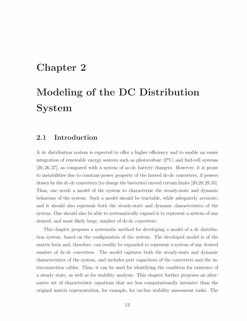
Fig. 2.2 shows a schematic diagram of the dc distribution system of Fig. 2.1. As
the diagram indicates, the central VSC is interfaced with the host ac power grid via
a three-phase tie reactor, Ls; the resistance Rs represents the aggregate effect of the
on-state power loss of the switches of the VSC and ohmic power loss of the tie reactor.
Each distribution wire/cable is represented by a corresponding series R−L branch. The
power leaving the network-side port of a dc-dc converter is denoted by Pdc, which can be
positive or negative for a battery charger, and only positive for a converter that interfaces
Page 32
2.2. System Configuration and Components 15
=
= =
=
dc-dc
converter #1
dc-dc
converter #2
=
= =
=
dc-dc
converter #3
dc-dc
converter #4
=
=
dc-dc
converter #n
central VSC
… …Host AC
Power
Grid
PV Modules
Management
Unit
electric power flow
communication flow
=
~
EV EV
EV
EV
Figure 2.1: A dc distribution system for power integration of electric vehicles and PVmodules.
PV modules.
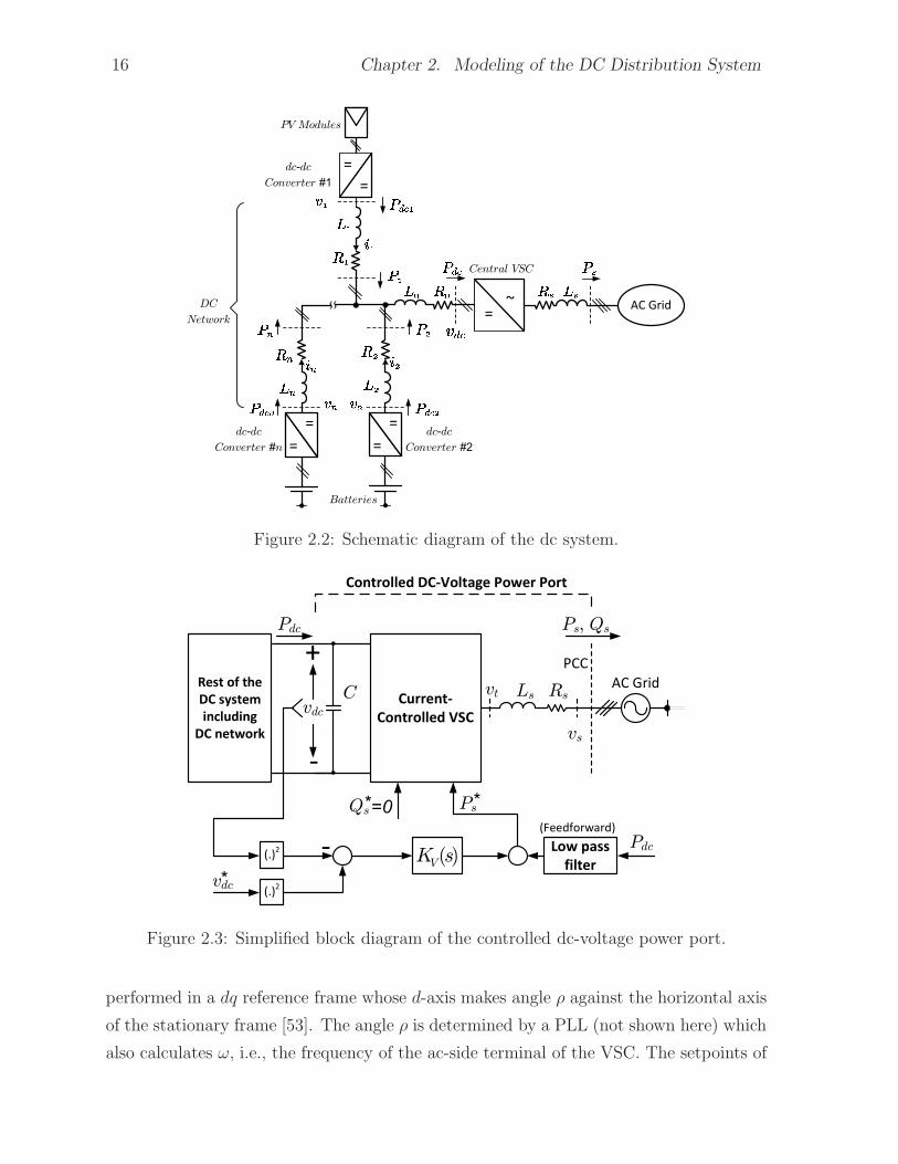
2.2.1 Central VSC
The central VSC and its control scheme act as a controlled dc-voltage power port and
regulate the dc voltage of the network (Fig. 2.3 illustrates the concept). The VSC is
current-controlled, such that its output real power, Ps, rapidly tracks the real-power
setpoint, P ∗s , issued by a dc-voltage regulation loop. Pdc denotes the power that the
rest of the dc system delivers to the VSC. As Fig. 2.3 indicates, a measure of Pdc
is incorporated in the control loop, as a feed-forward signal, to mitigate the dynamic
coupling between the dc-voltage regulation loop and the rest of the dc system.
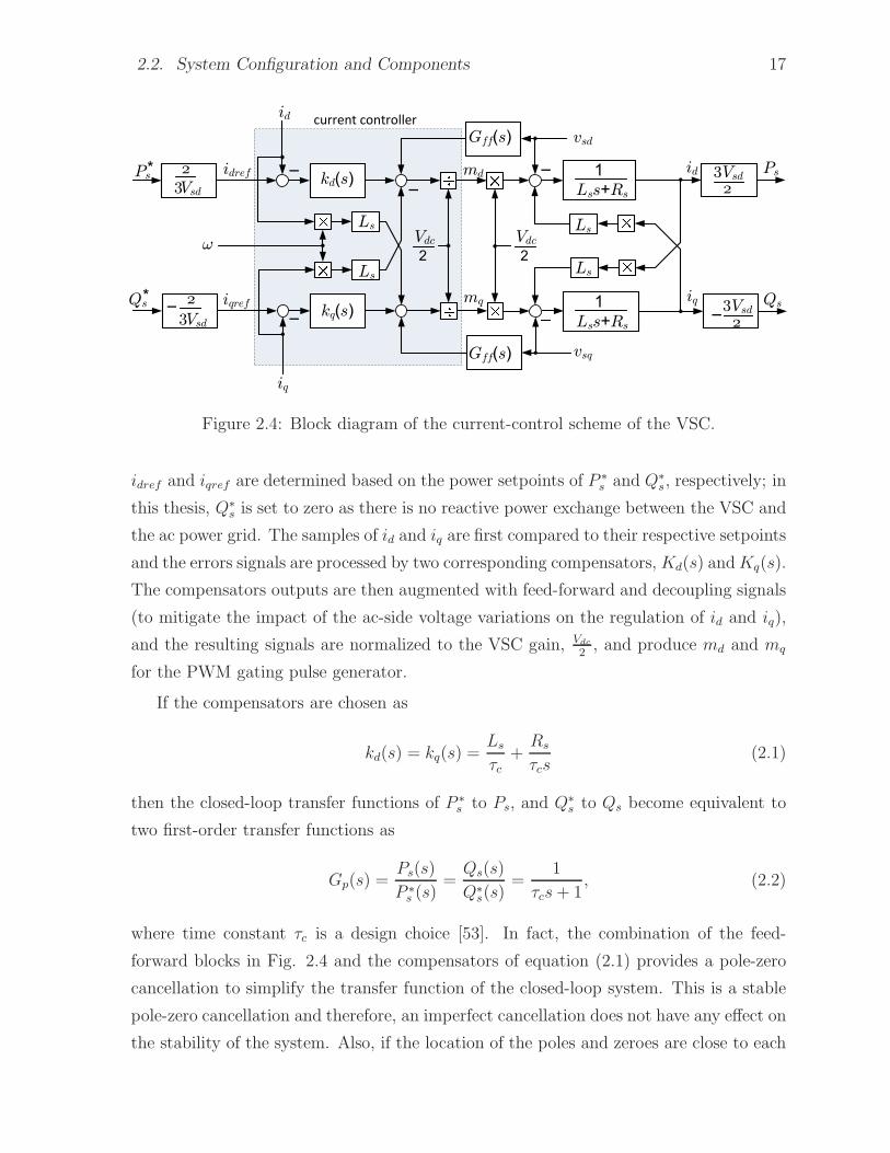
Current-Controlled Scheme
The function of the current-control scheme is to regulate the ac-side current of the VSC,
by means of the pulse-width modulation (PWM) switching strategy. Fig. 2.4 illustrates
a block diagram of the current-control scheme. As Fig. 2.4 indicates, the control is
Page 33
16 Chapter 2. Modeling of the DC Distribution System
AC Grid
~
=
=
=
=
=
=
=
~~
Central VSC
PV Modules
DC
Network
Batteries
dc-dc
Converter #1
dc-dc
Converter #n
dc-dc
Converter #2
Figure 2.2: Schematic diagram of the dc system.
AC GridCurrent-
Controlled VSC
Rest of the
DC system
including
DC network
PCC+
-
- Low pass
filter
(Feedforward)
Pdc
RsLsvt
vs
vdc
Ps*Qs*=0
C
Pdc Ps, Qs
*vdc
Controlled DC-Voltage Power Port
(.)2
(.)2
)(sKV
Figure 2.3: Simplified block diagram of the controlled dc-voltage power port.
performed in a dq reference frame whose d-axis makes angle ρ against the horizontal axis
of the stationary frame [53]. The angle ρ is determined by a PLL (not shown here) which
also calculates ω, i.e., the frequency of the ac-side terminal of the VSC. The setpoints of
Page 34
2.2. System Configuration and Components 17
kd (s)
Ls
id
idref
ω
Ps*
Vsd
vsd
id
Gff (s)
Ls
−
kq (s)
Ls
iq
iqref iq
Gff (s)
Ls
vsq
Vsd−
−
−
Vdc2
Vdc2
Qs*
− Vsd
Vsd
−Qs
Psmd
mq
current controller
1Lss+Rs
1Lss+Rs
Figure 2.4: Block diagram of the current-control scheme of the VSC.
idref and iqref are determined based on the power setpoints of P ∗s and Q∗
s, respectively; in
this thesis, Q∗s is set to zero as there is no reactive power exchange between the VSC and
the ac power grid. The samples of id and iq are first compared to their respective setpoints
and the errors signals are processed by two corresponding compensators, Kd(s) andKq(s).
The compensators outputs are then augmented with feed-forward and decoupling signals
(to mitigate the impact of the ac-side voltage variations on the regulation of id and iq),
and the resulting signals are normalized to the VSC gain, Vdc
2, and produce md and mq
for the PWM gating pulse generator.
If the compensators are chosen as
kd(s) = kq(s) =Ls
τc+
Rs
τcs(2.1)
then the closed-loop transfer functions of P ∗s to Ps, and Q∗
s to Qs become equivalent to
two first-order transfer functions as
Gp(s) =Ps(s)
P ∗s (s)
=Qs(s)
Q∗s(s)
=1
τcs+ 1, (2.2)
where time constant τc is a design choice [53]. In fact, the combination of the feed-
forward blocks in Fig. 2.4 and the compensators of equation (2.1) provides a pole-zero
cancellation to simplify the transfer function of the closed-loop system. This is a stable
pole-zero cancellation and therefore, an imperfect cancellation does not have any effect on
the stability of the system. Also, if the location of the poles and zeroes are close to each
Page 35
18 Chapter 2. Modeling of the DC Distribution System
Power Controller
DynamicsDC-bus Voltage
Compensator
−0vdc~Ps
~* Ps
~
Kv (s) Gp (s) sC( )
Gf (s)
Cs
Pdc~
Composite Control Plant
ev (s) uv(s) dcs +1
Ge (s)
Gv (s)
Figure 2.5: Control block diagram of dc-bus voltage controller.
other, the imperfect stable pole-zero cancellation creates a very short trace in the root-
locus diagram of the system that have little impact on the behavior of the closed-loop
system.
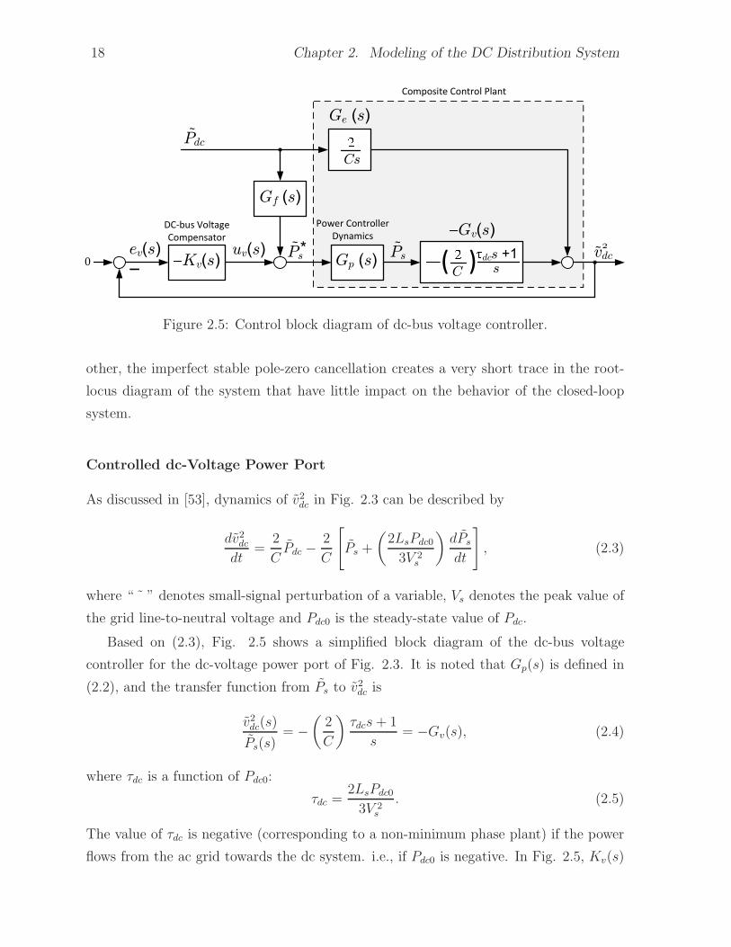
Controlled dc-Voltage Power Port
As discussed in [53], dynamics of v2dc in Fig. 2.3 can be described by
dv2dcdt
=2
CPdc −
2
C
[
Ps +
(
2LsPdc0
3V 2s
)
dPs
dt
]
, (2.3)
where “ ˜ ” denotes small-signal perturbation of a variable, Vs denotes the peak value of
the grid line-to-neutral voltage and Pdc0 is the steady-state value of Pdc.
Based on (2.3), Fig. 2.5 shows a simplified block diagram of the dc-bus voltage
controller for the dc-voltage power port of Fig. 2.3. It is noted that Gp(s) is defined in
(2.2), and the transfer function from Ps to v2dc is
v2dc(s)
Ps(s)= −
(
2
C
)
τdcs+ 1
s= −Gv(s), (2.4)
where τdc is a function of Pdc0:
τdc =2LsPdc0
3V 2s
. (2.5)
The value of τdc is negative (corresponding to a non-minimum phase plant) if the power
flows from the ac grid towards the dc system. i.e., if Pdc0 is negative. In Fig. 2.5, Kv(s)
Page 36
2.2. System Configuration and Components 19
is multiplied by −1 to compensate for the negative sign of Gv(s).
Fig. 2.5 also indicates that a measure of Pdc is incorporated in the control process
through a feed-forward filter, Gf (s), to weaken the dynamic linkage between the the
dc-voltage control loop and the rest of the dc system. The transfer function from Pdc,
which is considered as a disturbance, to v2dc is
v2dc(s)
Pdc
=Ge(s)−Gf(s)Gp(s)Gv(s)
1 +Kv(s)Gp(s)Gv(s). (2.6)
To have a perfect cancelation of the dynamic linkage between the the dc-voltage
control loop and the rest of the dc system, one should choose Gf (s) as
Gf(s) =Ge(s)
Gp(s)Gv(s)=
1
Gp(s) (τdcs+ 1). (2.7)
However, as mentioned in this section, the value of τdc will be negative if the power flows
from the ac grid towards the dc system, which in turn, leads to a right-half pole (RHP)
for the transfer function (2.7), and the system will lose the internal stability. In [53],
Gf(s) was chosen as an unity. Thus, to have a good disturbance rejection performance,
i.e., to minimize the dynamic coupling between Pdc and v2dc, one needs an adequately
large controller gain for Kv(s) [55].
Fig. 2.6 shows the general form of the dc-voltage controller, Kv(s), which can be
written as
Kv(s) =k0sH1(s)H2(s) (2.8)
where H1(s), andH2(s) are lead filters to increase phase margin of the closed-loop system.
The reason for using two lead filters is that by increasing the controller gain, k0, to have
a better disturbance rejection performance, the required phase shift to ensure the stable
operation of the system also will be increased. Each lead filter, as described in [53], can
provide a maximum of 90 of phase shift. Therefore, for a total phase shift of more than
90, two lead filters will be needed.
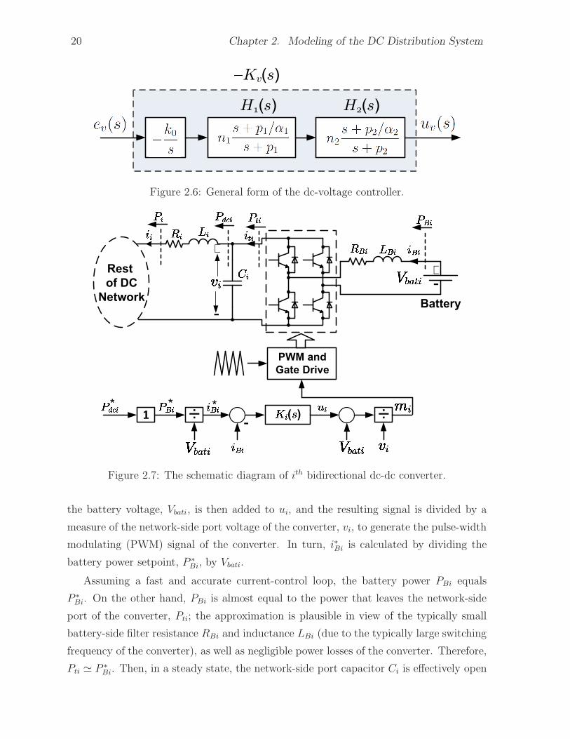
2.2.2 dc-dc Converters
Fig. 2.7 shows a simplified schematic diagram of a full-bridge dc-dc converter which, with
no loss of generality, is assumed to represent a battery charger. The battery current, iBi,
is regulated at its setpoint, i∗Bi, by a feedback control loop in which a compensator,
Ki(s), processes the error (i∗Bi − iBi) and generates the control signal ui. A measure of
Page 37
20 Chapter 2. Modeling of the DC Distribution System
Kv (s)
H (s) H (s)
Figure 2.6: General form of the dc-voltage controller.
+
−
Rest
of DC
NetworkBattery
+−
( ) ÷−÷ *
PWM and
Gate Drive
**1
Figure 2.7: The schematic diagram of ith bidirectional dc-dc converter.
the battery voltage, Vbati, is then added to ui, and the resulting signal is divided by a
measure of the network-side port voltage of the converter, vi, to generate the pulse-width
modulating (PWM) signal of the converter. In turn, i∗Bi is calculated by dividing the
battery power setpoint, P ∗Bi, by Vbati.
Assuming a fast and accurate current-control loop, the battery power PBi equals
P ∗Bi. On the other hand, PBi is almost equal to the power that leaves the network-side
port of the converter, Pti; the approximation is plausible in view of the typically small
battery-side filter resistance RBi and inductance LBi (due to the typically large switching
frequency of the converter), as well as negligible power losses of the converter. Therefore,
Pti ≃ P ∗Bi. Then, in a steady state, the network-side port capacitor Ci is effectively open
Page 38
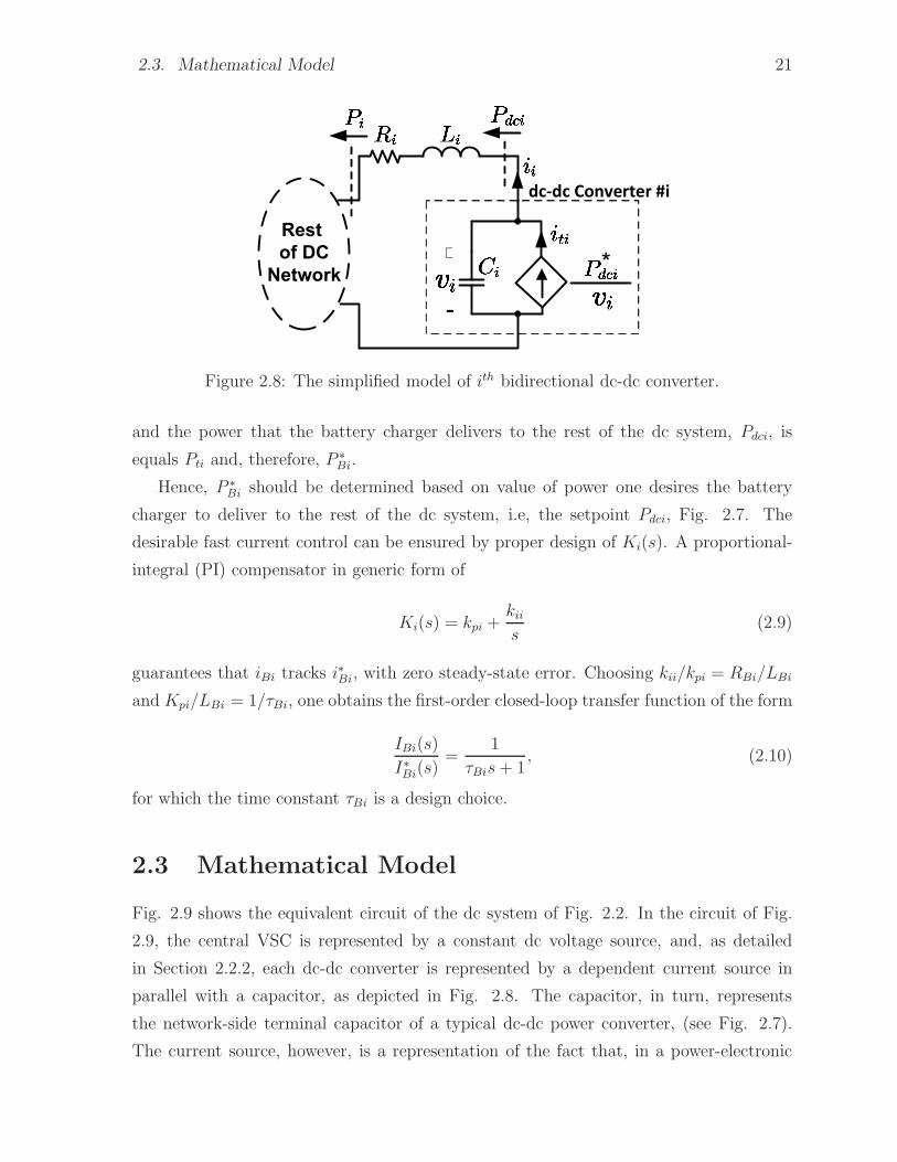
2.3. Mathematical Model 21
dc-dc Converter #i
+
−
Rest
of DC
Network*
Figure 2.8: The simplified model of ith bidirectional dc-dc converter.
and the power that the battery charger delivers to the rest of the dc system, Pdci, is
equals Pti and, therefore, P∗Bi.
Hence, P ∗Bi should be determined based on value of power one desires the battery
charger to deliver to the rest of the dc system, i.e, the setpoint Pdci, Fig. 2.7. The
desirable fast current control can be ensured by proper design of Ki(s). A proportional-
integral (PI) compensator in generic form of
Ki(s) = kpi +kiis
(2.9)
guarantees that iBi tracks i∗Bi, with zero steady-state error. Choosing kii/kpi = RBi/LBi
and Kpi/LBi = 1/τBi, one obtains the first-order closed-loop transfer function of the form
IBi(s)
I∗Bi(s)=
1
τBis+ 1, (2.10)
for which the time constant τBi is a design choice.
2.3 Mathematical Model
Fig. 2.9 shows the equivalent circuit of the dc system of Fig. 2.2. In the circuit of Fig.
2.9, the central VSC is represented by a constant dc voltage source, and, as detailed
in Section 2.2.2, each dc-dc converter is represented by a dependent current source in
parallel with a capacitor, as depicted in Fig. 2.8. The capacitor, in turn, represents
the network-side terminal capacitor of a typical dc-dc power converter, (see Fig. 2.7).
The current source, however, is a representation of the fact that, in a power-electronic
Page 39
22 Chapter 2. Modeling of the DC Distribution System
...
...
dc-dc
converter #1
+
−
*
dc-dc
converter #2
+
−
*
dc-dc
converter #3
+
−
*
dc-dc
converter #n
+
−
*
Figure 2.9: Equivalent circuit of the dc system of Fig. 2.2.
converter with regulated output (battery current, PV array voltage, etc.), the network-
side port power does not depend on the network-side port voltage. Thus, the value of
the current for the ith, (i = 1, 2, ..., n), converter is
iti =1
viP ∗dci (2.11)
where P ∗dci and vi are the power setpoint and network-side terminal voltage of the con-
verter, respectively. For a converter serving as a battery charger, P ∗dci is the setpoint
for the power delivered by (i.e., discharging) the battery; a negative value for P ∗dci, thus,
corresponds to a charging power. For a converter interfacing PV modules, P ∗dci can only
be positive and is determined by a so-called maximum power-point tracking (MPPT)
algorithm, to equal the maximum power that the PV modules can deliver at the pre-
vailing sunlight and temperature conditions. Thus, the assumption is that the control of
the dc-dc converter is fast and, therefore, the power exchanged with the battery, or that
delivered by the PV modules, equals P ∗dci. For a dc-dc converter with a voltage-droop
mechanism, the modeling process has been presented in In Appendix A.
Let us regard the dc bus of the system of Fig. 2.9 as a node, i.e., the per-unit-length
inductance and resistance of the bus are ignored (the model without this assumption is
presented in Section 2.5). Thus, the following family of differential equations describe
dynamics of the dc system of Fig. 2.9:
−vi +Riii + Li
diidt
+ L0
n∑
k=1
dikdt
+R0
n∑
k=1
ik + vdc = 0, (2.12)
Ci
dvidt
=P ∗dci
vi− ii, (2.13)
Page 40
2.3. Mathematical Model 23
where i = 1, 2, ..., n.
Rewriting (2.12) in the matrix form, one finds
−v +Rbi+ Lb
di
dt+ L0
di
dt+R0i + vdc = 0 (2.14)
where
v =
v1
v2...
vn
, i =
i1
i2...
in
, vdc = vdc
1
1...
1
n×1
, (2.15)
and
Lb =
L1 0 · · · 0
0 L2 · · · 0...
.... . .
...
0 0 · · · Ln
, Rb =
R1 0 · · · 0
0 R2 · · · 0...
.... . .
...
0 0 · · · Rn
, (2.16)
L0 =
L0 L0 · · · L0
L0 L0 · · · L0
......
. . ....
L0 L0 · · · L0
n×n
, R0 =
R0 R0 · · · R0
R0 R0 · · · R0
......
. . ....
R0 R0 · · · R0
n×n
. (2.17)
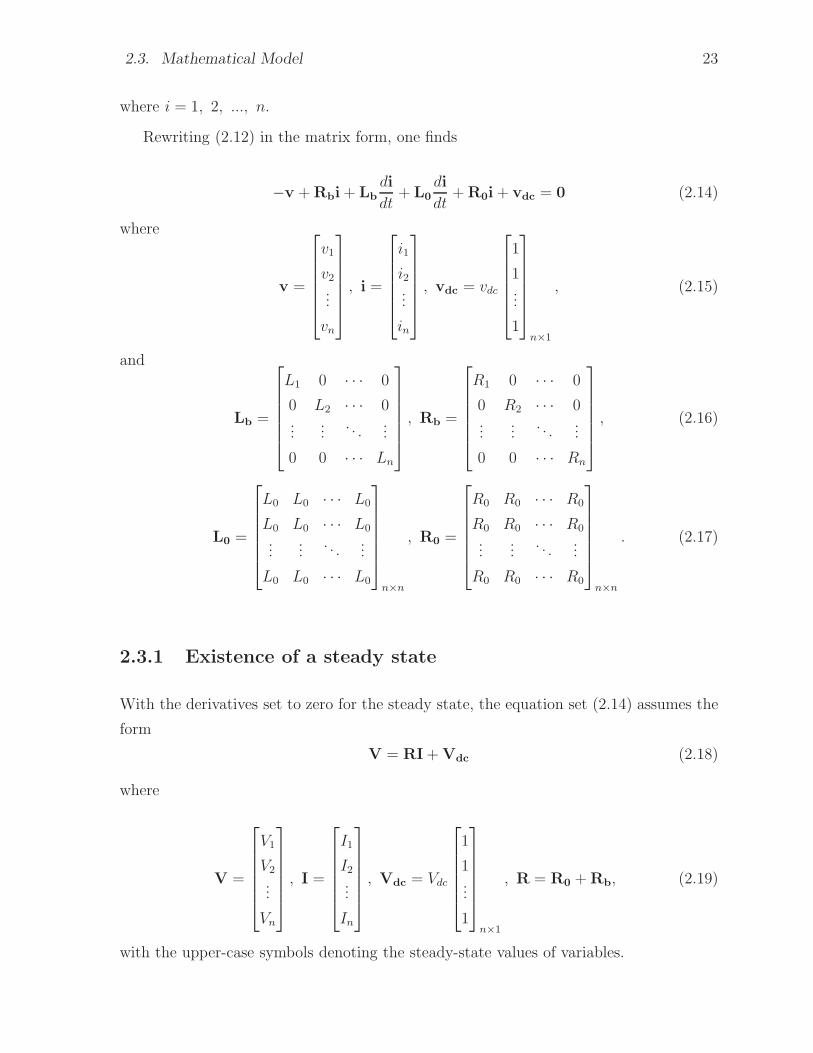
2.3.1 Existence of a steady state
With the derivatives set to zero for the steady state, the equation set (2.14) assumes the
form
V = RI+Vdc (2.18)
where
V =
V1
V2
...
Vn
, I =
I1
I2...
In
, Vdc = Vdc
1
1...
1
n×1
, R = R0 +Rb, (2.19)
with the upper-case symbols denoting the steady-state values of variables.
Page 41
24 Chapter 2. Modeling of the DC Distribution System
Pre-multiplication of (2.18) by IT , the transpose of I, yields
ITV = ITRI+ ITVdc (2.20)
and
PT = ITV
=
n∑
i=1
ViIi
=n∑
i=1
P ∗dci
= ITRI+ ITVdc, (2.21)
where PT is the sum of the powers leaving the network-side ports of all dc-dc converters.
Equation (2.21) describes the steady-state power flow in the dc system. The term
ITRI is the total power dissipated in the network cables, and ITVdc is the power that
enters the dc port of the central VSC and flows to the ac grid. The extreme value of PT
can be found by setting the derivative of (2.21) with respect to I to zero:
∂PT
∂I
∣
∣
∣
∣
I=Iext
= 2RIext +Vdc = 0 (2.22)
which implies
Iext = −1
2R−1Vdc. (2.23)
It can then be shown that the second derivative of (2.21) is 2R. If Ri 6= 0 (i =
1, 2, ..., n), then R is symmetric and positive-definite (see Appendix B for proof) and,
therefore, also nonsingular. Hence, 2R is also a positive-definite matrix and, thus, PT is
minimum for the current given by (2.23), Iext. Substituting for Iext from (2.23) in (2.21),
one finds
PT,min = −1
4VT
dcR−1Vdc, (2.24)
where PT,min is the minimum of PT and is always negative.
Equation (2.24) gives the minimum of PT for a real-valued set of currents. In other
words, if PT is smaller than PT,min, i.e., if the power collectively absorbed by the dc-dc
converters exceeds the absolute value of PT,min, then the power loss of the dc network
becomes excessive and (2.21) fails to yield a real-valued solution. Thus, if a steady state
Page 42
2.3. Mathematical Model 25
exists, the following inequality holds:
PT ≥ PT,min. (2.25)
Inequality (2.25) represents a necessary condition for the existence of a steady state
for the dc system. Thus, a steady state does not exist if the aggregate power absorbed by
the dc-dc converters is greater than the absolute value of PT,min. However, if inequality
(2.25) holds, one cannot guarantee the existence of a steady state for the system. It is
also interesting to note that for a single-source/single-load resistive circuit, the absolute
value of the right-hand side of (2.25) is the maximum power that can be transferred to
the load, corresponding to the case of the source Thevenin resistance being equal to the
load resistance.
2.3.2 State-space model
Linearizing the equation set (2.13), one finds
Ci
dvidt
= −P ∗dci
V 2i
vi − ii (2.26)
where “ ˜ ” denotes small-signal perturbation of a variable, and Vi is the steady-state
value of vi.
Rewriting equation sets (2.12) and (2.26) in the matrix form, one obtains
Ldi
dt= −Ri+ v (2.27)
Cdv
dt= −i−Pv (2.28)
where
L = L0 + Lb, (2.29)
and
C =
C1 0 · · · 0
0 C2 · · · 0...
.... . .
...
0 0 · · · Cn
, P =
P ∗
dc1
V 2
1
0 · · · 0
0P ∗
dc2
V 2
2
· · · 0...
.... . .
...
0 0 · · ·P ∗
dcn
V 2n
. (2.30)
Page 43
26 Chapter 2. Modeling of the DC Distribution System
If Ci 6= 0 and Li 6= 0 (i = 1, 2, ..., n), then C and L are symmetric, positive-definite
(see Appendix B), and, therefore, nonsingular matrices.
Equations (2.27) and (2.28) can be combined into a classical state-space form as
x = Ax (2.31)
where
x =
[
i
v
]
2n×1
, A =
[
−L−1R L−1
−C−1 −C−1P
]
2n×2n
. (2.32)
Matrix A can be expressed as
A =
[
−L−1 0n×n
0n×n −C−1
][
R −In×n
In×n P
]
= N−1M (2.33)
where
N =
[
−L 0n×n
0n×n −C
]
, M =
[
R −In×n
In×n P
]
, (2.34)
and N is a symmetric, negative-definite (and, therefore, non-singular) matrix.
For stability analysis, one must evaluate the eigenvalues of A in (2.31). Let λ be an
eigenvalue of A. Then one can write
Aw = λw, w 6= 0, (2.35)
where w is an eigenvector of A, associated with λ. Substituting for A in (2.35) from
(2.33), one finds
N−1Mw = λw. (2.36)
Pre-multiplying (2.35) by N, one obtains
Mw = λNw, (2.37)
Calculating the conjugate transpose of (2.37), one finds
wMT = λwN, (2.38)
where λ is the complex conjugate of λ, w is the adjoint of w, and MT is the transpose
Page 44
2.3. Mathematical Model 27
of M.
Pre-multiplying both sides of (2.37) by w, and post-multiplying both sides of (2.38) by
w, one finds
wMw = λwNw (2.39)
wMTw = λwNw. (2.40)
Adding the corresponding sides of (2.39) and (2.40), one concludes
w(
M+MT)
w = 2Re(λ)wNw. (2.41)
In (2.41), N is a real, symmetric, negative-definite matrix. Therefore, the real part
of λ is negative if(
M+MT)
is a positive-definite matrix.
w(
M+MT)
w =[
w1 w2
]
[
2R 0n×n
0n×n 2P
][
w1
w2
]
(2.42)
= 2w1Rw1 + 2w2Pw2 (2.43)
where
w =
[
w1
w2
]
. (2.44)
As mentioned earlier, R is a positive-definite matrix and, based on (2.35) and (2.44),
w1 andw2 cannot both be zero. Therefore,(
M+MT)
is positive-definite if P is positive-
definite. Hence, the dc system is stable if P is positive-definite:
P > 0 ⇒ Re(λ) < 0. (2.45)
Since P is a diagonal matrix, it is positive-definite if its diagonal elements are all
positive, i.e., if the dc-dc converters all deliver power to the dc system. However, it
should be pointed out that the inequality (2.45) is a sufficient condition for stability
of the dc system. Thus, one cannot comment on the stability of the dc system if P is
positive-semidefinite, negative-definite, or indefinite, i.e., if some converters absorb power.
Therefore, to evaluate the stability of the dc system, one must evaluate the eigenvalues
of A, as explained next.
Page 45
28 Chapter 2. Modeling of the DC Distribution System
Equation (2.37) can be rewritten as
(M− λN)w = 0, w 6= 0. (2.46)
Substituting for M andN from (2.34) in (2.46), one can arrive at the following expression
for the determinant of M− λN, which, in turn, is the characteristic equation associated
with (2.31):∣
∣
∣
∣
∣
R+ λL −In×n
In×n P+ λC
∣
∣
∣
∣
∣
= 0, (2.47)
which can be rewritten as [56]
∣
∣
∣(R+ λL)(P+ λC) + In×n
∣
∣
∣= 0. (2.48)
Let us now express (2.48) in the form
∣
∣
∣
∣
∣
∣
∣
∣
∣
∣
∣
α1 + β1 α2 · · · αn
α1 α2 + β2 · · · αn
......
. . ....
α1 α2 · · · αn + βn
∣
∣
∣
∣
∣
∣
∣
∣
∣
∣
∣
= 0 (2.49)
where
αi = λ2L0Ci + λ
(
R0Ci +P ∗dci
V 2i
L0
)
+P ∗dci
V 2i
R0 (2.50)
and
βi = λ2LiCi + λ
(
RiCi +P ∗dci
V 2i
Li
)
+
(
1 +P ∗dci
V 2i
Ri
)
. (2.51)
It can then be shown (see Appendix C) that (2.49) is equivalent to the 2nth-order poly-
nomial equationn∏
i=1
βi +n∑
i=1
(αi
n∏
k = 1
k 6= i
βk) = 0 , (2.52)
which is remarkably easier to solve, from a computational burden standpoint, relative to
a direct calculation of the eigenvalues of A (i.e., using matrix operations); this facilitates
physical implementation of the method on an embedded signal-processing platform.
A special case deserves some inspection: let R0 and L0 be zero. Then, matrices R
Page 46
2.3. Mathematical Model 29
and L are diagonal and, therefore, R+ λL takes the form
R+ λL =
R1 + λL1 0 · · · 0
0 R2 + λL2 · · · 0...
.... . .
...
0 0 · · · Rn + λLn
. (2.53)
Since C and P are diagonal matrices, (2.48) can be rewritten as
∣
∣
∣
∣
∣
∣
∣
∣
∣
(R1 + λL1)(
P ∗
dc1
V 2
1
+ λC1
)
+ 1 · · · 0...
. . ....
0 · · · (Rn + λLn)(
P ∗
dcn
V 2n
+ λCn
)
+ 1
∣
∣
∣
∣
∣
∣
∣
∣
∣
= 0 (2.54)
andn∏
k=1
[
(Rk + λLk)
(
P ∗dck
V 2k
+ λCk
)
+ 1
]
= 0. (2.55)
Equation (2.55) implies that the dc system is stable if the power setpoint of each dc-dc
converter satisfies the corresponding following two constraints:
P ∗dck > −
V 2k
Rk
, (2.56)
and
P ∗dck > −
RkCkV2k
Lk
, (k = 1, 2, ..., n). (2.57)
It should be pointed out that, typically, (2.57) is the ruling constraint.
The foregoing conclusion is expected in view of the fact that the special case corre-
sponds to a dc system that consists of n independently energized dc-dc converters, and
it is important as it enables one to gain insights into the impact of parameters on the
stability, in general. For example, one can expect the stability to improve as larger ca-
pacitances are chosen for the dc-dc converters, whereas larger network inductances are
detrimental to the stability. Further, (2.57) indicates that larger line resistances improve
the stability. However, an increase in resistances is not a remedial option as the power
loss in the system will also increase. Therefore, to overcome this problem, an active
damping method has been proposed in [40] to virtually increase the resistance while
avoiding physical resistances. An increase in the dc voltage level of the system also im-
proves the stability, as (2.57) indicates. However, a higher dc voltage level has safety and
Page 47
30 Chapter 2. Modeling of the DC Distribution System
-
+
-
+
Figure 2.10: Realistic battery model.
operational implications and, naturally, translates into a higher cost.
2.4 Simulation Results
To demonstrate the accuracy of the developed model, the equation set (2.31)-(2.32),
hereafter referred to as the “linear model”, is numerically solved in the MATLAB software
environment, and the response predicted by it is compared with the response obtained
from a detailed switched model of the dc system, Fig. 2.2, in the PSCAD/EMTDC
software environment. The parameters used for simulation studies and model validation
are given in Appendix D, unless otherwise is mentioned.
The study dc system includes six dc-dc converters, one for a PV system and the
remainder for five vehicles. The network-side current of the PV system converter is
represented by i1, whereas i2 through i6 signify the network-side currents of the vehicle
converters (battery chargers).
2.4.1 Realistic Battery Model
The battery in Fig. 2.7 has been modeled by an ideal voltage source. Figure 2.10 shows
a more realistic model of a Li-ion battery [57]. The model consists of a dc voltage source,
Voc to represent the open-circuit voltage of the battery, a series resistor, Rser, and two
RC parallel network, (Rtrs, Ctrs) and (Rtrl, Ctrl) to model the transient behavior of the
battery. It can be assumed that the value of the resistors and capacitors in the model
are constant over the SOC range of 20% to 100% [57].
To build a battery module with high voltage and capacity, multiple low-voltage, low-
capacity battery cells should be connected in series and parallel. In this thesis, the voltage
of the battery module in the PEVs is considered to be 320 V. Therefore, using a 4.1 V,
0.85 Ah battery cell, 78 battery cells must be connected in series to form a branch and
Page 48
2.4. Simulation Results 31
build the voltage (Ncell ser = 78). To increase the battery capacity, multiple branches
are needed to be connected in parallel. Thus, for a typical 40 kWh battery module, 147
branches are needed (Nbranch par = 147). To find the parameters of the realistic model
for the battery module, one can use the following equations [58]
Voc(module) = Ncell serVoc(cell), Rser(module) =Ncell ser
Nbranch par
Rser(cell),
Rtrs(module) =Ncell ser
Nbranch par
Rtrs(cell), Ctrs(module) =Nbranch par
Ncell ser
Ctrs(cell),
Rtrl(module) =Ncell ser
Nbranch par
Rtrl(cell), Ctrl(module) =Nbranch par
Ncell ser
Ctrl(cell).
Table 2.1 lists the parameters of a 4.1 V, 850-mAh TCL PL-383562 Li-ion battery
cell which is the building block of a 320 V, 40 kWh battery module [57]. As Table 2.1
indicates, the time constants RtrsCtrs and RtrlCtrl for the battery module are 31.8 s and
219.2 s, respectively. These time constant values are very large comparing to the time
scale of the network-side dynamics of the dc-dc converter, and therefore, their impact on
the transient behavior of the dc-dc converter is negligible. Fig. 2.11 shows the responses of
a battery charger to a step change in the power setpoint from 0 to -10 kW. The responses
have been illustrated for two cases: (i) when the battery has been modeled by an ideal
voltage source of 320 V, and (ii) when the battery has been modeled by a realistic battery
model of Fig. 2.10 with parameters of Table 2.1. In this test, at t = 0.8 s, the power
setpoint of the battery charger is changed from 0 to -10 kW, meaning that the battery is
started to being charged. As Fig. 2.11 shows, although there are some discrepancies in
battery voltage, Vbat1, between realistic model and the ideal voltage source, the battery
current, iB1, and the power between the battery charger and the rest of dc system, Pdc2,
are almost identical for two cases. In fact, due to constant-power property of the dc-dc
converter, the battery voltage fluctuations don’t have any impact on the network-side
dynamics of the converter as depicted in Fig. 2.11, and therefore, hereafter in this thesis,
the ideal voltage source will be used to model the batteries. It should also be noted that
in commercially-available standard chargers on the market, the maximum charging or
discharging power of the battery is a function of the battery voltage which is a function
of length of charging or discharging. However, as the power setpoint of the battery
charger is updated infrequently, this is not a source of instability in this thesis. A more
sophisticated treatment would still result in a monotonically changing value and hence
Page 49
32 Chapter 2. Modeling of the DC Distribution System
Table 2.1: Parameters of a typical battery cell and battery moduleParameter Battery cell Battery module
Nominal Voltage (V) Voc 4.1 320Capacity (Ah) Bcap 0.85 125Internal resistance (mΩ) Rser 74 39Transient Rtrs 46 24resistances (mΩ) Rtrl 49 26Transient Ctrs 703 1326capacitances (F) Ctrl 4475 8433
316
318
320
322
324
Vbat1(V
)
Ideal voltage sourceBattery model
−32
−31.5
−31
−30.5
−30
i∗ B1(A
)
Ideal voltage sourceBattery model
−60−50−40−30−20−10
0102030
i B1(A
)
Ideal voltage sourceBattery model
0.8 0.805 0.81 0.815 0.82 0.825 0.83
−25
−20
−15
−10
−5
0
5
Pdc2
(kW
)
time (s)
Ideal voltage sourceBattery model
Figure 2.11: Response of a battery charger for two models for the battery: ideal voltagesource and realistic battery model.
would still not affect stability.
2.4.2 Case 1: Stable Pre- and Post-Disturbance Operation
Initially, the dc system is in a steady state, while the PV system delivers 50 kW (through
Converter #1), the first vehicle absorbs 10 kW (via Converter #2), the second and third
electric vehicles deliver 20 kW each, and the remaining two vehicles absorb 20 kW each.
Then at t = 1.3 s, the power setpoint of Converter #2 is changed stepwise from −10
kW to −20 kW. Fig. 2.12 depicts the responses of the variables i1, i2, i3, and Pdc2, and
demonstrating a close agreement between the linear and detailed models. Fig. 2.12 also
shows that, as assumed, vdc remains tightly regulated about its pre-disturbed steady-state
Page 50
2.4. Simulation Results 33
100
105
110
i 1(A
)
linear modelswitched model
−60
−50
−40
−30
−20
i 2(A
)
linear modelswitched model
35
40
45
i 3(A
)
linear modelswitched model
−30
−25
−20
−15
−10
Pdc2
(kW
)
linear modelswitched model
1.3 1.305 1.31 1.315 1.32 1.325 1.33 1.335 1.34
478
479
480
481
482
vdc
(V)
time (s)
switched model
Figure 2.12: Response of the dc-system to a change in Pdc2 from −10 kW to −20 kWwhen Pdc1 is 50 kW and Pdc3 to Pdc6 are −20 kW.
value.
Fig. 2.13 shows the results of another test, one in which Converter #3 (corresponding
to the second vehicle) delivers power to the rest of the dc system. In this case, the dc
system is initially in a steady state, while the PV system produces 50 kW, Converter #2
absorbs 50 kW, Converter #3 delivers 20 kW, and every other converter absorbs 20 kW.
Then, the power setpoint of Converter #3 is changed stepwise from 20 kW to 30 kW, at
t = 1.3 s. Fig. 2.13 illustrates a close agreement between the linear and detailed models
in predicting the responses of i1, i2, i3, and Pdc3.
2.4.3 Case 2: Sensitivity to Cable Length
To evaluate the sensitivity to the length of the interconnection cables, an eigenvalue anal-
ysis has been conducted using the linear model, and Fig. 2.14 illustrates the dependence
of the dominant eigenvalues of the dc system on the network cable length. In this case,
the PV system generates a power of 10 kW, Converter #2 absorbs 70 kW, and every
other converter absorbs 60 kW. Thus, the length of the cables, connecting the dc bus
to the central VSC and the dc-dc converters, are increased from 100 m to 500 m. As
illustrated in Fig. 2.14, the eigenvalues move toward the imaginary axis if the length of
Page 51
34 Chapter 2. Modeling of the DC Distribution System
100
105
110
i 1(A
)
linear modelswitched model
−110
−105
−100i 2
(A)
linear modelswitched model
40
50
60
70
80
i 3(A
)
linear modelswitched model
15
20
25
30
35
Pdc3
(kW
)
linear modelswitched model
1.3 1.305 1.31 1.315 1.32 1.325 1.33 1.335 1.34
478
479
480
481
482
vdc
(V)
time (s)
switched model
Figure 2.13: Response of the dc-system to a change in Pdc3 from 20 kW to 30 kW whenPdc1 is 50 kW and Pdc2 is −50 kW and Pdc4 to Pdc6 are −20 kW.
−35 −30 −25 −20 −15 −10 −5 0 5
−3000
−2000
−1000
0
1000
2000
3000
jw
σ
Increase in cable length
Increase in cable length
Figure 2.14: Eigenvalue migration plot as a function of the length of the interconnectioncables.
the interconnection cables increase.
2.4.4 Case 3: Sensitivity to Network-Side Capacitances
Fig. 2.15 illustrates the dependance of the stability of the dc system on the network-side
capacitances of the converters. For this case, it is assumed that the PV system delivers 10
kW, Converter #2 absorbs 80 kW, and any other converter absorbs 70 kW. Thus, three
Page 52
2.4. Simulation Results 35
−60 −50 −40 −30 −20 −10 0−2500
−2000
−1500
−1000
−500
0
500
1000
1500
2000
2500
jw
σ
Increase in capacitance
Increase in capacitance
Figure 2.15: Eigenvalue migration plot as a function of network-side capacitance.
dominant pairs of eigenvalues have been marked on the complex plane for the network-
side capacitances equally ranging from 2000 µF to 5000 µF . As Fig. 2.15 shows, the
eigenvalues move away from the imaginary axis as the network-side capacitances increase,
indicating the stabilizing effect of the network-side capacitances.
2.4.5 Case 4: Sensitivity to Power Absorption
Fig. 2.16 illustrates the migration of the dominant pair of eigenvalues (i.e., the pair
with the real part smallest in absolute value), as the power absorbed by Converter #2
is increased, for three different values of network-side capacitances of the converters. It
is assumed for this case that the PV system generates 10 kW, while, except Converter
#2, each converter absorbs 70 kW. Thus, the eigenvalue loci are mapped on the complex
plane for the power of Converter #2 ranging from −20 kW to −80 kW. As Fig. 2.16 indi-
cates, irrespective of the value of the network-side capacitances, the eigenvalues approach
the imaginary axis as the power absorbed by Converter #2 increases. This study case
illustrates what is well known as the destabilizing effect of the so-called constant-power
loads [20], [28], [59], [40]- [60].
Fig. 2.16 also indicates that the maximum amount of power that Converter #2 can
absorb before the system becomes unstable decrease as the network-side capacitances are
made smaller. This is consistent with the findings of Fig. 2.15.
Page 53
36 Chapter 2. Modeling of the DC Distribution System
−80 −70 −60 −50 −40 −30 −20 −10 0
−2100
−1500
−1000
−500
0
500
1000
1500
2100
jw
σ
Increase in power absorption
Increase in power absorption
Ci = 2 mFCi = 3 mFCi = 4 mFCi = 5 mF
Figure 2.16: Eigenvalue migration plot as a function of power consumption by dc-dcconverter#2.
2.4.6 Case 5: Unstable Post-Disturbance Operation
In the last study case, the dc system is assumed to initially be in a steady state, with the
PV system generating 10 kW, Converter #2 absorbing 60 kW, and every other converter
absorbing 70 kW. Moreover, each converter has a network-side capacitance of 2000 µF .
Then, the power setpoint of Converter#2 is changed stepwise from −60 kW to −80 kW,
at t = 1.3 s. As previously illustrated by Figs. 2.15 and 2.16, the new set of powers results
in a pair of imaginary eigenvalues, about ± 2100j rad/s, and, consequently, destabilizes
the system, as Fig. 2.17 indicates. It is observed that the period of oscillations is about
3 ms (≃ 2π/2100 s), confirming that the linear and detailed models closely agree.
2.5 dc System with Multiple Nodes of Coupling
Fig 2.18 illustrates a configuration where no common node of coupling exists, but the
converters are connected to the network at different corresponding nodes of coupling;
the impedance between two adjacent nodes is represented by the series connection of an
inductance, Lbi, and a resistance, Rbi.
The dynamics of the system of Fig. 2.18 are governed by the following differential
Page 54
2.5. dc System with Multiple Nodes of Coupling 37
−220
−200
−180
−160
−140
−120
i 2(A
)
linear modelswitched model
−100
−90
−80
−70
−60
−50
Pdc2
(kW
)
linear modelswitched model
1.3 1.302 1.304 1.306 1.308 1.31 1.312 1.314 1.316 1.318 1.32
472
474
476
478
480
482
484
vdc
(V)
time (s)
switched model
Figure 2.17: Response of the dc-system to a change in Pdc2 from −60 kW to −80 kWwhen Pdc1 is 10 kW, and Pdc3 to Pdc6 are −70 kW.
equations:
− vi +Riii + Li
diidt
+Rb1
n∑
k=1
ik + Lb1
n∑
k=1
dikdt
(2.58)
+ ...+Rbi
n∑
k=i
ik + Lbi
n∑
k=i
dikdt
+ vdc = 0,
for i = 1, 2, ..., n− 1, and
− vn +Rnin + Ln
dindt
+Rb1
n∑
k=1
ik + Lb1
n∑
k=1
dikdt
+ ...+Rb(n−1)
n∑
k=n−1
ik + Lb(i−1)
n∑
k=n−1
dikdt
dt+ vdc = 0,
Ci
dvidt
=P ∗dci
vi− ii, i = 1, 2, ..., n. (2.59)
Page 55
38 Chapter 2. Modeling of the DC Distribution System
+
−
+
−
dc-dc
converter #1
+
−
**+
−
...
...
dc-dc
converter #2
dc-dc
converter #3
dc-dc
converter #n
* *
Figure 2.18: Equivalent circuit of the dc system with different nodes of coupling.
Linearizing (2.58) and (2.59), and expressing the resulting equations in the matrix
form, one finds
Lm
di
dt= −Rmi+ v (2.60)
Cdv
dt= −i−Pv (2.61)
where
Lm = Ln + Lb, (2.62)
Rm = Rn +Rb, (2.63)
Ln =
Lb1 Lb1 Lb1 · · · Lb1
Lb1 Lb1 + Lb2 Lb1 + Lb2 · · · Lb1 + Lb2
Lb1 Lb1 + Lb2
∑3i=1 Lbi · · ·
∑3i=1 Lbi
......
.... . .
...
Lb1 Lb1 + Lb2
∑3i=1 Lbi · · ·
∑n−1i=1 Lbi
Lb1 Lb1 + Lb2
∑3i=1 Lbi · · ·
∑n−1i=1 Lbi
, (2.64)
Rn =
Rb1 Rb1 Rb1 · · · Rb1
Rb1 Rb1 +Rb2 Rb1 +Rb2 · · · Rb1 +Rb2
Rb1 Rb1 +Rb2
∑3i=1Rbi · · ·
∑3i=1Rbi
......
.... . .
...
Rb1 Rb1 +Rb2
∑3i=1Rbi · · ·
∑n−1i=1 Rbi
Rb1 Rb1 +Rb2
∑3i=1Rbi · · ·
∑n−1i=1 Rbi
, (2.65)
Page 56
2.6. Conclusion 39
and Lb, Rb, C, and P have been defined by (2.16) and (2.30), respectively.
It can be shown that Rm and Lm are positive-definite matrices. Therefore, one can
employ the same approach as the one presented in Sections 2.3.1 and 2.3.2 to find a
state-space model for the system.
2.6 Conclusion
A systematic method was presented for developing a model of a dc distribution system,
based on the configuration of the system. The dc distribution system is assumed to host
electric vehicles and photovoltaic (PV) modules, using dc-dc converters, and integrates
them with an ac power grid. The developed model is of the matrix form and, therefore,
can readily be expanded to represent a dc distribution system of any desired number of dc-
dc converters. The model captures both the steady-state and dynamic characteristics of
the system, and includes port capacitors of the converters, as well as the interconnection
cables. Thus, it can be used for identifying the condition for existence of a steady
state, as well as for stability analysis. Furthermore, an alternative set of characteristic
equations was proposed that are less computationally intensive than the original matrix
representation, for example, for on-line stability assessment tasks. The adequacy of
the proposed model was demonstrated through a number of case studies conducted and
compared in PSCAD/EMTDC and MATLAB software environments.
Page 57
Chapter 3
Stability Enhancement of the DC
Distribution System
3.1 Introduction
The dc distribution systems embedding dc-dc converters are prone to instability due to
constant-power property of the dc-dc converters [28], [35]; the system becomes unstable if
the powers absorbed by the battery chargers exceed certain values [20]. This phenomenon
inflicts a limit on the maximum power that can be imported to charge the batteries
and, consequently, precludes full utilization of the installed capacities and prolongs the
charging times. Therefore, it is imperative to
1. systematically characterize the phenomenon and identify the prevailing constraints,
and
2. devise a stability enhancement technique, in order to push the limits and expand
the stable operating region of the dc system.
Expanding upon the idea proposed in [36], this chapter proposes a control technique
for expanding the stable operating region of a dc distribution system integrating PHEVs
via bidirectional dc-dc converters (battery chargers), such that the dc system and its
PHEVs can import larger powers from the host ac grid. The proposed technique is sim-
ple, does not require information internal to the system or its embedded converters, and
does not need hardware modifications. Rather, it only employs local measurements and
individual power setpoints and, therefore, can be exercised in a decentralized fashion.
40
Page 58
3.2. System Configuration 41
These, in turn, permit the use of commercially available dc-dc converters (battery charg-
ers), expected to further reduce the overall cost of the system. The proposed technique
is also applicable to other dc distribution systems, e.g., shipboard power systems, that
have multiple power-electronic converters.
3.2 System Configuration
Fig. 3.1 illustrates a dc distribution system, for example, in a parking lot, that hosts
PHEVs and photovoltaic (PV) modules. In this system, dc-dc converters are utilized as
battery chargers for the PHEVs and also for interfacing the PV modules. Moreover, a
central voltage-sourced converter (VSC) interfaces the dc distribution system to the host
ac grid. A communication network [61] is used to enable the exchange of metering and
control information for a management unit, to and from the dc-dc converters and the
central VSC. The management unit calculates the limits of the power exchange setpoints
and sends them to the dc-dc converters, to ensure that the dc system operates in its
stable operation region. The PHEV owners, on the other hand, can set state-of charge
(SOC) limits for their vehicles, to permit power exchanges only if the SOC resides within
a certain range. For example, if the SOC is above 70%, then energy can be sold to the rest
of the system, whereas if the SOC is below 40%, then the vehicle should buy energy from
the rest of the system. The aforementioned limits (determined based on the trip plans,
electricity price, and other factors) translate into power setpoints for the corresponding
dc-dc converters. For example, for a PHEV with 20 kWh of battery capacity, if the SOC
limit for energy export is 70% and the present SOC is 85%, then 3 kWh (that is, 15% of
the battery capacity) can be sold by the PHEV to the rest of the system, meaning that
the power setpoint of this particular PHEV can be set to export 9 kW of power in 20
minutes, or 3 kW of power in one hour, and so on [20].
Fig. 3.2 shows a simplified schematic diagram of the dc system. As the diagram
indicates, the dc system consists of a central VSC, a network of RL branches representing
the dc distribution network, and a multitude (3, here) of dc-dc power electronic converters
that represent either the battery chargers of the PHEVs or the power-electronic interface
of the PV system. The central VSC is interfaced with the host ac power grid via a
three-phase tie reactor with a per-phase inductance of Ls; the resistance Rs represents
the aggregate effect of the ohmic power losses of the tie reactor and conduction power
losses of the VSC. The central VSC regulates the dc voltage of the network. The PHEV
Page 59
42 Chapter 3. Stability Enhancement of the DC Distribution System
=
=
=
=
=
=
Host AC
Power
Grid
=
~
DC Distribution Network
=
=
=
=
…
…
Communication
Network
Central Voltage-Sourced
Converter
DC-DC
Converter
DC-DC
ConverterDC-DC
Converter
DC-DC
Converter
DC-DC
Converter
PV Modules
Management
Unit
Figure 3.1: A dc bus for distribution of power in a parking lot for PHEVs.
battery chargers can draw or deliver power, the PV system delivers power, and the host
ac grid compensates for any generation-consumption power mismatch, via the central
VSC. A study system, whose parameters is reported in Appendix E, is used for stability
analysis and performance evaluation in this chapter.
3.3 Mathematical Model
3.3.1 Central VSC
The central VSC and its control scheme act as a controlled dc-voltage power port, [53],
and regulate the dc voltage of the network (Fig. 3.3 illustrates the concept). The VSC
is current-controlled, such that its output real power, Ps, rapidly tracks the real-power
setpoint, P ∗s , issued by a dc-voltage regulation loop (in this chapter, variables with su-
perscript * signifies the setpoints). Pdc denotes the power that the rest of the dc system
delivers to the VSC. As Fig. 3.3 indicates, a measure of Pdc is incorporated in the control
loop, as a feed-forward signal, to mitigate the dynamic coupling between the dc-voltage
regulation loop and the rest of the dc system.
As discussed in [53] and also in Chapter 2 of this thesis, the transfer function from
Page 60
3.3. Mathematical Model 43
sR sLAC Grid
~
=
L R
=
=
1R
1L
=
=
=
=
3R
3L
~~
2R
2L
3vvvv
1v
2v
1i
2i
3i
Central VSC
PV Modules
DC-DC
Converter
DC-DC
Converter
DC-DC
Converter
DC
Network
Batteries
PPdc
PP
Ps
PPV
PPHEVPPHEV
Figure 3.2: Schematic diagram of the dc system.
AC GridCurrent-
Controlled VSC
Rest of the
DC system
including
DC network
PCC+
-
- Low pass
filter
(Feedforward)
Pdc
RsLsvt
vs
vdc
Ps*Qs*=0
C
Pdc Ps, Qs
*vdc
Controlled DC-Voltage Power Port
(.)2
(.)2
)(sKV
Figure 3.3: Simplified block diagram of the controlled dc-voltage power port.
Ps to vdc is
Gv(s) =v2dc(s)
Ps(s)= −
(
2
C
)
τs + 1
s, (3.1)
Page 61
44 Chapter 3. Stability Enhancement of the DC Distribution System
where the time constant τ is a function of the steady-state value of Pdc, i.e., Pdc0:
τ =2LsPdc0
3V 2s
, (3.2)
where Vs is the peak value of vs, the line-to-neutral voltage of ac grid at the point of
common coupling (PCC). As discussed in [53], τ is negative (corresponding to a non-
minimum phase plant) if Pdc0 is negative. Therefore, the dc-voltage regulation loop
should be tuned for a case where the maximum amount of power flows from the ac grid
towards the dc system to ensure stability also in other operating conditions.
In the remainder of this chapter, it is assumed that the controlled dc-voltage power
port of Fig. 3 rapidly and tightly regulates vdc at its setpoint v∗dc, irrespective of the
steady-state value or transient excursions of Pdc; it is assumed that the dynamics of vdc
decay to zero rapidly.
3.3.2 dc-dc converters
The PHEV batteries exchange energy with the dc system through corresponding bidirec-
tional dc-dc power-electronic converters which are referred, hereafter, to as the battery
chargers. Fig. 3.4 shows a simplified schematic diagram of a full-bridge dc-dc converter
which, with no loss of generality, is assumed to represent a battery charger (e.g., for the
ith PHEV of the dc system). The battery current, iBi, is regulated at its setpoint, i∗Bi, by
a feedback control loop in which a compensator, Ki(s), processes the error (i∗Bi− iBi) and
generates the control signal ui. A measure of the battery voltage, Vbati, is then added to
ui, and the resulting signal is divided by a measure of the network-side terminal voltage
of the converter, vi, to generate the pulse-width modulating (PWM) signal of the con-
verter. In turn, i∗Bi is calculated by dividing the battery power setpoint, P ∗Bi, by Vbati.
Assuming a fast and accurate current-control loop, the battery power PBi equals
P ∗Bi. On the other hand, PBi is almost equal to the power that leaves the network-side
port of the converter, Pti; the approximation is plausible in view of the typically small
battery-side filter resistance RBi and inductance LBi (due to the typically large switching
frequency of the converter), as well as negligible power losses of the converter. Therefore,
Pti ≃ P ∗Bi. Then, in a steady state, the terminal capacitance Ci is effectively open and
the power that the battery charger delivers to the rest of the dc system, PPHEV i, is equals
Pti and, therefore, P∗Bi.
Page 62
3.3. Mathematical Model 45
+
−
Rest
of DC
NetworkBattery
+−
( ) ÷−÷ *
PWM and
Gate Drive
**1
Figure 3.4: Schematic diagram of the bidirectional dc-dc converter as a battery chargerfor ith PHEV.
Hence, P ∗Bi should be determined based on value of power one desires the battery
charger to deliver to the rest of the dc system, i.e, the setpoint PPHEV i, Fig. 3.4. The
desirable fast current control can be ensured by proper design of Ki(s). For example, as
discussed in Chapter 2, if Ki(s) is of the proportional-integral (PI) type, then its gains
can be determined for a first-order closed-loop transfer function of the form
IBi(s)
I∗Bi(s)=
1
τBis+ 1, (3.3)
for which the time constant τBi is a design choice.
The current that leaves the positive network-side terminal of the converter is iti =
Pti/vi, which based on the conclusion that Pti ≃ P ∗Bi = P ∗
PHEV i, can be written as
iti =1
viP ∗PHEV i. (3.4)
Hence, from its network-side port, the converter can be represented by a dependent
current source whose value is iti = P ∗PHEV i/vi, as shown in Fig. 3.5. If P ∗
PHEV i is an
exogenous signal, i.e., if it does not depend on any other variable of the dc system, then Pti
is constant (from the viewpoint of dynamics) and, therefore, the converter presents itself
as a constant-power element to the external world; any change in vi is counteracted by
a corresponding change in iti, such that Pti remains constant at P ∗PHEV i. This constant-
Page 63
46 Chapter 3. Stability Enhancement of the DC Distribution System
DC-DC Converter
+
−
Rest
of DC
Network*
Figure 3.5: Simplified model of the dc-dc converter.
PV Modules
3C+
−2C
+
−
Battery Charger
1C
+
−
1i 2
i3i
**
Battery Charger
Figure 3.6: Equivalent circuit for the analysis of the dc system of Fig. 3.2.
power property of regulated power-electronic converters is known for giving rise to system
instabilities, [29], as also demonstrated in Section 3.4.
In a PV system, the power-electronic interface is internally regulated so as to maintain
the dc voltage of its host modules at a value that corresponds to the maximum- power
point (MPP) under the prevailing sunlight and temperature conditions. Therefore, the
model of Fig. 3.5 can be used also for a PV system, except that P ∗PHEV i is replaced with
PPV,mpp. Based on aforementioned discussions, Fig. 3.6 represents the equivalent circuit
of the dc system of Fig. 3.2; P ∗PHEV i represents the power exchange setpoint of the ith
battery charger, and PPV,mpp signifies the maximum power of a PV array as imposed by
the corresponding maximum powerpoint tracking (MPPT) scheme.
Based on Fig. 3.6, the following nonlinear differential equations describe the dynamic
Page 64
3.4. Stability Enhancement 47
behavior of the dc system of Fig. 3.2:
Ld(i1 + i2 + i3)
dt+ L1
di1dt
= v1 − vdc
−R(i1 + i2 + i3)− R1i1,
(3.5)
L1di1dt
− L2di2dt
= v1 − v2 −R1i1 +R2i2, (3.6)
L2di2dt
− L3di3dt
= v2 − v3 −R2i2 +R3i3, (3.7)
C1dv1dt
=P ∗PHEV 1
v1− i1, (3.8)
C2dv2dt
=P ∗PHEV 2
v2− i2, (3.9)
C3dv3dt
=PPV,mpp
v3− i3. (3.10)
The steady-state values of the variables of the system can be calculated by setting the
derivatives to zero in (3.5) through (3.10), and solving the nonlinear equations for every
given set of power exchange setpoints P ∗PHEV 1, P
∗PHEV 2, and PPV,mpp.
The linearized state-space representation of (3.5) through (3.10) can be expressed by
x = Ax, (3.11)
where x = [i1 i2 i3 v1 v2 v3]T is the vector of state variables, and ˜ denotes small-
signal perturbation around steady-state operating points, and components of A can be
determined based on resistance and inductance of the cables, the capacitance of the
converters, and steady-state operating point of the converters. The state-space model of
(3.11) can be used for stability analysis of the dc system and in section 3.4, it will be
shown that the dc system is prone to instability when the battery chargers are drawing
energy from the ac power grid.
3.4 Stability Enhancement
Constant-power elements have been shown to have detrimental effects on the stability of
their host dc distribution systems, if the direction of flow from the distribution system
towards the constant-power elements [20], [28], [29]. Thus, to identify the boundary be-
Page 65
48 Chapter 3. Stability Enhancement of the DC Distribution System
−100 −90 −85 −70 −60 −50 −40 −30 −20 −10−100
−90
−80
−70
−60
−50
−40
−30
−20
−10
Stable Region
Unstable Region
PP
HE
V2
(kW
)
PPHEV 1 (kW )
Figure 3.7: Stable and unstable regions in the charging mode.
tween the stable and unstable regions associated with the study system, an algorithm
has been executed in Matlab software environment, such that for any given set of power
exchange setpoints PPHEV 1 and PPHEV 2, the linearized state-space model has been ex-
amined in terms of stability, and the boundary between the stable and unstable operating
regions has been depicted in Fig. 7, when the PV system generates an aggregate power
of 10 kW.
It is observed that the system becomes unstable if the power absorbed by the bat-
tery chargers exceed the levels marked by the boundary curve. The instability, in turn,
prevents the battery chargers from operating at their full capacities and, consequently,
results in under-utilization of the investment and prolongs the charging times.
To mitigate the aforementioned instability issue, a filtered version of the network-
side voltage of each dc-dc converter is used to alter the power exchange setpoint of the
converter, as illustrated in Fig. 3.8. Thus, the power exchange setpoint of the ith dc-dc
converter, P ∗Bi, is determined by the following nonlinear equations:
P ∗Bi =
(
viwi
)
P ∗PHEV i, (3.12)
Page 66
3.4. Stability Enhancement 49
( ) ÷−÷ **×÷
*
Figure 3.8: Modification of the power exchange setpoints of the dc-dc converters.
÷+
−
Rest
of DC
Network*
Figure 3.9: Simplified model of the modified dc-dc converter.
dwi
dt=
vi − wi
τi, (3.13)
where τi and wi are the time constant and the filtered measure of the network-side dc
voltage, vi, respectively.
Fig. 3.9 shows a simplified model of the modified dc-dc converter.
The current that flows to the dc system, iti, can be found as
iti =1
wi
P ∗PHEV i. (3.14)
As illustrated in Section 3.6, if τi is large compared to time scale of dynamics of
interconnection cables in the dc network then the instability of the dc system can be
avoided in all operating points of the system. The steady-state gain of the filter that
converts vi to wi is unit, therefore, the modification of (3.12) will not change the steady-
state operating point of the dc-dc converter. It should be pointed out that, as Fig. 3.10
shows, the proposed technique modifies the power exchange setpoints of the converters,
Page 67
50 Chapter 3. Stability Enhancement of the DC Distribution System
Figure 3.10: Connection block diagram for the proposed technique.
using local measurements. Thus, it does not require access to any variables internal to
the converters, does not need hardware or software modifications, and can be exercised in
a decentralized fashion. Therefore, it can be implemented using commercially available
battery chargers.
By applying the proposed modification in Fig. 3.8 to the dc-dc converters of the
system of Fig. 3.2, equations (3.8) through (3.10) are replaced by the following differential
equations.
C1dv1dt
=P ∗PHEV 1
w1− i1, (3.15)
dw1
dt=
v1 − w1
τ1, (3.16)
C2dv2dt
=P ∗PHEV 2
w2− i2, (3.17)
dw2
dt=
v2 − w2
τ2, (3.18)
C2dv3dt
=PPV,mpp
w3− i3, (3.19)
dw3
dt=
v3 − w3
τ3. (3.20)
The linearized versions of (3.5) through (3.7), and (3.15) through (3.20) can be expressed
in the state-space form as
xmod = Amodxmod, (3.21)
where xmod = [i1 i2 i3 v1 w1 v2 w2 v3 w3]T is the new vector of state variables, and the
Page 68
3.4. Stability Enhancement 51
matrix Amod is introduced by (3.22) and (3.23); the uppercase letters denote the steady-
state values of the state variables, which can be calculated by setting the derivatives to
zero in equations (3.5) through (3.7), and (3.15) through (3.20).
Amod =
RL2L3+R1(LL2+LL3+L2L3)−den
RL2L3−R2LL3
−denRL2L3−R3LL2
−den
RL1L3−R1LL3
−den
RL1L3+R2(LL1+LL3+L1L3)−den
RL1L3−R3LL1
−den
RL1L2−R1LL2
−denRL1L2−R2LL1
−den
RL1L2+R3(LL1+LL2+L1L2)−den
− 1C1
0 0
0 0 0
0 − 1C2
0
0 0 0
0 0 − 1C3
0 0 0
L(L2+L3)+L2L3
den0 LL3
−den0 LL2
−den0
LL3
−den0 L(L1+L3)+L1L3
den0 LL1
−den0
LL2
−den0 LL1
−den0 L(L1+L2)+L1L2
den0
0 −P ∗
PHEV 1
V 2
1C1
0 0 0 0
1τ1
− 1τ1
0 0 0 0
0 0 0 −P ∗
PHEV 2
V 2
2C2
0 0
0 0 1τ2
− 1τ2
0 0
0 0 0 0 0 −PPV,mpp
V 2
3C3
0 0 0 0 1τ3
− 1τ3
(3.22)
den = LL1L2 + LL1L3 + LL2L3 + L1L2L3. (3.23)
Stability of the modified system has been checked for the study system in Matlab
software environment. Fig. 3.11 shows the boundaries between the stable and unstable
operating regions for different values of τi. In this case, the PV system is generating a
power of 10 kW and power consumption of PHEVs are variable. Fig. 3.11 depicts that if
the values of τi increase then the stable operating region of the dc system expands. This
agrees with the analysis presented in Section 3.6.
Page 69
52 Chapter 3. Stability Enhancement of the DC Distribution System
−110 −100 −90 −80 −70 −60 −50 −40 −30 −20 −10
−110
−100
−90
−80
−70
−60
−50
−40
−30
−20
−10
Stable Region
UnstableRegion
PP
HE
V2
(kW
)
PPHEV 1 (kW )
Unmodified systemModified system (τi = 0.1 ms)Modified system (τi = 0.2 ms)Modified system (τi = 0.3 ms)
Figure 3.11: Boundaries between stable and unstable regions for unmodified and modifiedsystems with different values of τi.
It should be noted that an increase in the PV power generation slightly expands
the stable region, as Fig. 3.12 indicates. However, the improving effect of an increased
PV power generation is insignificant compared to the effect of the time constant in
the proposed modification. Moreover, PV power generation is not deterministic and,
therefore, one cannot rely on it to enhance the stability.
3.5 Simulation Results
The study system was simulated in the PSCAD/EMTDC software environment. Fig.
3.13 and Fig. 3.14 demonstrate the performance of the dc system in the normal conditions
when the steady-state operating point lies inside the stable region.
Initially, the system is in a steady state and, as Fig. 3.13 shows, the controlled dc-
voltage power port regulates vdc at 480 V. At t = 0.5 s, the PV system starts to generate
a power of 20 kW. At t = 0.6 s, the batteries in PHEV2 start to absorb a power of 20
kW, as indicated by P ∗PHEV 2, and at t = 0.7 s, the batteries in PHEV1 start to charge
with a power of 30 kW, as indicated by P ∗PHEV 1. Therefore, in a steady state, a power of
Page 70
3.5. Simulation Results 53
−100 −90 −85 −70 −60 −50 −40 −30 −20 −10−100
−90
−80
−70
−60
−50
−40
−30
−20
−10
Stable Region
Unstable Region
PP
HE
V2
(kW
)
PPHEV 1 (kW )
PV generation= 10 kWPV generation= 50 kWPV generation= 100 kW
Figure 3.12: Boundaries between stable and unstable regions for different values of powergeneration of PV modules.
about 30 kW flows from the ac power grid to the dc system. As Fig. 3.13 illustrates, the
dc system remains stable under the aforementioned sequence of events and the central
VSC regulates the vdc at 480 V.
Fig. 3.14 shows the system performance for a case where the power flow is from the
dc system towards the ac power grid. The PV system starts to generate a power of 20
kW at t = 0.5 s, as Fig. 3.14 shows. At t = 0.6 s, the batteries in PHEV2 start to
consume a power of 20 kW that compensates the PV system generation so no power
flows to the ac power grid. At t = 0.7 s, the batteries in PHEV1 start to generate 30
kW, as indicated by P ∗PHEV 1 in Fig. 3.14. Consequently, in a steady state, a power of
around 30 kW flows from the dc system to the ac power grid. The dc system remains
stable and vdc is regulated at 480 V for all of the aforementioned disturbances.
Fig. 3.15 and Fig. 3.16 demonstrate the effectiveness of the proposed modification to
enhance the stability of the dc distribution system. Performance of the system has been
has been analyzed in two working scenarios. In the first scenario, as Fig. 3.15 shows,
the system is working at an operating point where the power consumptions of PHEV1
and PHEV2 are 60 kW and 50 kW, respectively, and the PV system generates a power
Page 71
54 Chapter 3. Stability Enhancement of the DC Distribution System
−30
−20
−10
0
PP
HE
V1(k
W)
PB1
PPHEV 1
P ∗
PHEV 1
−20
−10
0P
PH
EV
2(k
W)
PB2
PPHEV 2
P ∗
PHEV 2
0
10
20
PP
V(k
W)
−60
−40
−20
0
20
40
Ps(k
W)
0.5 0.55 0.6 0.65 0.7 0.75
478
479
480
481
vdc(V
)
time(s)
Figure 3.13: The dc system response when the power flows from the ac power grid to thedc system.
−10
0
10
20
30
PP
HE
V1(k
W)
PB1
PPHEV 1
P ∗
PHEV 1
−20
−10
0
PP
HE
V2(k
W)
PB2
PPHEV 2
P ∗
PHEV 2
0
10
20
PP
V(k
W)
−20
0
20
40
Ps(k
W)
0.5 0.55 0.6 0.65 0.7 0.75
479
479.5
480
480.5
481
vdc(V
)
time(s)
Figure 3.14: The dc system response when the power flows from the dc system to the acpower grid.
of 10 kW. Based on Fig. 3.11, this operating point situates at the verge of instability
for the unmodified dc system. Thus, a change in the power consumption of PHEV1, at
Page 72
3.6. Stability Enhancement for a dc System with Single dc-dc Converter 55
t = 1.3 s, from 60 kW to 77 kW, leads to instability for the unmodified dc system while
for the modified dc systems with both τi = 0.1 ms, τi = 0.2 ms, and τi = 2 ms, the
systems remain stable and converge to the new setpoints. The instability first occurs to
P1, P2, and P3, while the dc-dc converters try to keep the power levels of PHEV1 and
PHEV2 constant at their setpinots. The central VSC keeps the dc voltage, vdc, constant.
In the second scenario, as Fig. 3.16 shows, the system works at another operating
point where the power consumptions of PHEV1 and PHEV2 are 60 kW and 50 kW,
respectively, and the PV system generates 10 kW. A change in the power consumption
of PHEV1, at t = 1.3 s, from 60 kW to 85 kw, moves the operating point outside
of the stable region for the unmodified dc system and the modified dc system with
τi = 0.3 ms, as predicted in Fig 3.11. Fig. 3.16 shows that this transition destabilizes
both the unmodified dc system and the modified dc system with τi = 0.1 ms, whereas the
modified dc-dc converters with τi = 0.2 ms and τi = 2 ms remains stable and converge
to the new setpoints. The instabilities in this case also first occur to P1, P2, and P3.
Figs. 3.15 and 3.16 show that, the response settles more rapidly at its post-disturbance
value as the the time constant τi is increased.
Fig. 3.15(a) and Fig. 3.16(a)(b) might give the impression that the instability does
not have any impact on the dc voltage. However, this is not the reality and is due to
the fact that the simulation results in Fig. 3.15 and Fig. 3.16 have been shown for a
relatively short period of time, for the sake of clarity of the waveforms; the growth of
oscillations becomes more obvious if one shows the waveforms over a longer time slot.
Fig. 3.17 presents long-run simulations for both scenarios. As depicted in the figure,
in both scenarios the dc voltage starts to oscillate and eventually crashes due to the
instability of the dc system. However, in the first scenario, the oscillations start after a
longer time, compared to the second scenario, due to the larger distance of its operating
point relative to the borderline between the stable and unstable regions.
3.6 Stability Enhancement for a dc System with Sin-
gle dc-dc Converter
Fig. 3.18 illustrates the application of the proposed modification to a circuit consisting
of a dc voltage source, an interconnection line, and a constant-power element. In the
circuit of Fig. 3.18, E represents the source voltage, L and R respectively signify the
line inductance and resistance, and C denotes the line-side terminal capacitance of the
Page 73
56 Chapter 3. Stability Enhancement of the DC Distribution System
−110
−90
−77−70−60−50
PP
HE
V1
(kW
)
PPHEV1
P1
−80
−60
−50
−40
−20
PP
HE
V2
(kW
)
PPHEV2
P2
0
10
20
PP
V(k
W)
PPV
P3
1.3 1.35 1.4 1.45
477
478
479
480
481
482
vdc
(V)
time (s)
(a)
PPHEV1
P1
PPHEV2
P2
PPV
P3
1.3 1.35 1.4 1.45time (s)
(b)
PPHEV1
P1
PPHEV2
P2
PPV
P3
1.3 1.35 1.4 1.45time (s)
(c)
PPHEV1
P1
PPHEV2
P2
PPV
P3
1.3 1.35 1.4 1.45time (s)
(d)
Figure 3.15: Responses of the dc system in the first scenario; (a) the unmodified dcsystem (b) the modified dc system with τi = 0.1 ms, (c) the modified dc system withτi = 0.2 ms, (d) the modified dc system with τi = 2 ms.
constant-power element.
The dynamics of the circuit of Fig. 3.18 are governed by the following differential
equations
Ldi
dt= −Ri+ v − E, (3.24)
τdw
dt= v − w, (3.25)
Cdv
dt= −i+
P ∗
w. (3.26)
It can be shown that the existence condition for steady-state operating point of the
system is
P ∗ ≥ −E2
4R. (3.27)
It also can be shown that the steady-state voltage of the constant-power element, V , is
Page 74
3.6. Stability Enhancement for a dc System with Single dc-dc Converter 57
−110−100
−85
−70−60−50
PP
HE
V1
(kW
)
PPHEV1
P1
−80
−60
−50
−40
−20
PP
HE
V2
(kW
)
PPHEV2
P2
0
10
20
PP
V(k
W)
PPV
P3
1.3 1.35 1.4 1.45
477
478
479
480
481
482
vdc
(V)
time (s)
(a)
PPHEV1
P1
PPHEV2
P2
PPV
P3
1.3 1.35 1.4 1.45time (s)
(b)
PPHEV1
P1
PPHEV2
P2
PPV
P3
1.3 1.35 1.4 1.45time (s)
(c)
PPHEV1
P1
PPHEV2
P2
PPV
P3
1.3 1.35 1.4 1.45time (s)
(d)
Figure 3.16: Responses of the dc system in the second scenario; (a) the unmodified dcsystem (b) the modified dc system with τi = 0.1 ms, (c) the modified dc system withτi = 0.2 ms, (d) the modified dc system with τi = 2 ms.
always greater than half of dc voltage source, E, for all operating points
V ≥E
2. (3.28)
The linearized form of (3.26) is
Cdv
dt= −i−
P ∗
V 2w. (3.29)
The eigenvalues of the linearized system can be found by solving the following char-
acteristic equation
LCτλ3 + (LC +RCτ) λ2 +
(
P ∗
V 2L+RC + τ
)
λ+P ∗
V 2R + 1 = 0. (3.30)
Based on Routh-Horwitz stability test, the system is stable if and only if
P ∗ > −V 2
R, (3.31)
Page 75
58 Chapter 3. Stability Enhancement of the DC Distribution System
1.3 1.35 1.4 1.45 1.5 1.55 1.6 1.65 1.7 1.75 1.8465
470
475
480
485
490
495
vdc
(V)
time (s)
1.3 1.35 1.4 1.45 1.5465
470
475
480
485
490
495
vdc
(V)
time (s)
Figure 3.17: Long-run simulations for vdc; the first unstable scenario for instability (top),the second unstable scenario for instability (bottom).
÷+
−
*E
Figure 3.18: Proposed modification on a single constant-power element.
and
P ∗ > −RCV 2
L−
τV 2
L, (3.32)
Page 76
3.6. Stability Enhancement for a dc System with Single dc-dc Converter 59
and
(LC +RCτ)
(
P ∗
V 2L+RC + τ
)
> LCτ
(
1 +P ∗
V 2R
)
. (3.33)
Considering (3.27) and (3.28), inequality (3.31) is always true for all operating points
of the system. If τ is chosen as
τ >L
R− RC, (3.34)
then one can write
−1
R> −
RC
L−
τ
L. (3.35)
Multiplying both sides of (3.35) by V 2, one obtains
−V 2
R> −
RCV 2
L−
τV 2
L. (3.36)
Comparing (3.31) and (3.36), one can conclude that by choosing τ as (3.34), the inequality
(3.32) is true for all operating points of the system.
Inequality (3.33) can be rewritten as
LC
(
P ∗
V 2L+RC + τ
)
+RCτ
(
P ∗
V 2L+RC + τ
)
> LCτ
(
1 +P ∗
V 2R
)
. (3.37)
First, let focus on the second term of the left hand side of (3.37) and its relation to the
right hand side of (3.37). Choosing τ as (3.34) one can write
RC + τ >L
R. (3.38)
Adding P ∗
V 2L to both side of (3.38), one obtains
RC + τ +P ∗
V 2L >
L
R+
P ∗
V 2L. (3.39)
Inequality (3.39) can be rewritten as
R
(
RC + τ +P ∗
V 2L
)
> L
(
1 +P ∗
V 2R
)
(3.40)
or
RCτ
(
RC + τ +P ∗
V 2L
)
> LCτ
(
1 +P ∗
V 2R
)
. (3.41)
Inequality (3.41) indicates that if τ is chosen as (3.34) then the second term of left hand
Page 77
60 Chapter 3. Stability Enhancement of the DC Distribution System
side of (3.37) is always greater than the left hand side of (3.37).
On the other hand, we already know that if τ is chosen as (3.34) then (3.32) is true.
Therefore, one can write
LC
(
P ∗
V 2L+RC + τ
)
> 0. (3.42)
Combining (3.41) and (3.42), one can conclude that (3.37) always holds, and therefore,
the system is always stable in its operating point range. This means that by choosing
a proper value for τ , based on parameters of the dc line, the proposed modification
stabilizes the dc system with the constant-power element.
As inequality (3.34) indicates, a dc system with larger network-side dc-dc converter
capacitances and/or smaller interconnection cable L/R ratios requires smaller values
for the time constant τi to ensure stability. In the other words, larger network-side
capacitances and smaller cable L/R ratios have stabilizing effects on the dc system.
3.7 Stability Enhancement for a dc System with n
dc-dc Converters
Fig. 3.19 illustrates the application of the proposed modification to a dc system with n
dc-dc converters for n PHEVs. Applying the same approach as of Section 2.3.2, one can
develop a state-space model for the modified system of Fig. 3.19 as the following:
xnew = Anewxnew, (3.43)
where
xnew =
i
v
w
3n×1
, i =
i1...
in
, v =
v1...
vn
, w =
w1
...
wn
. (3.44)
Matrix A can be expressed as
Anew =
−L−1R L−1 0n×n
−C−1 0n×n −C−1P
0n×n τ−1 −τ
−1
3n×3n
(3.45)
Page 78
3.7. Stability Enhancement for a dc System with n dc-dc Converters 61
÷+
−
*÷
+
−
*
÷+
−
*
...
...
Figure 3.19: Proposed modification on a dc system with n dc-dc converters.
where
τ =
τ1 0 · · · 0
0 τ2 · · · 0...
.... . .
...
0 0 · · · τn
, (3.46)
and
L =
L0 + L1 L0 · · · L0
L0 L0 + L2 · · · L0
......
. . ....
L0 L0 · · · L0 + Ln
, R =
R0 +R1 R0 · · · R0
R0 R0 +R2 · · · R0
......
. . ....
R0 R0 · · · R0 +Rn
(3.47)
C =
C1 0 · · · 0
0 C2 · · · 0...
.... . .
...
0 0 · · · Cn
, P =
P ∗
PHEV 1
V 2
1
0 · · · 0
0P ∗
PHEV 2
V 2
2
· · · 0...
.... . .
...
0 0 · · ·P ∗
PHEVn
V 2n
. (3.48)
Similar to (2.33), Anew can be rewritten as
Anew =
−L−1 0n×n 0n×n
0n×n −C−1 0n×n
0n×n 0n×n −τ−1
R −In×n 0n×n
In×n 0n×n P
0n×n −In×n In×n
= N−1new
Mnew (3.49)
Page 79
62 Chapter 3. Stability Enhancement of the DC Distribution System
where
Nnew =
−L 0n×n 0n×n
0n×n −C 0n×n
0n×n 0n×n −τ
, Mnew =
R −In×n 0n×n
In×n 0n×n P
0n×n −In×n In×n
. (3.50)
Assuming τi > 0, i = 1, 2, · · ·n, Nnew is a symmetric, negative-definite (and, there-
fore, non-singular) matrix.
For stability analysis, one must evaluate the eigenvalues of Anew in (3.43). Let λ be
an eigenvalue of Anew. Then one can write
Au = λu, u 6= 0, (3.51)
where u is an eigenvector of Anew, associated with λ. Substituting for Anew in (3.51)
from (3.49), one finds
Nnew−1Mnewu = λu. (3.52)
Pre-multiplying (3.52) by Nnew, one obtains
Mnewu = λNnewu, (3.53)
Equation (3.53) can be rewritten as
(Mnew − λNnew)u = 0, u 6= 0. (3.54)
Substituting for Mnew and Nnew from (3.50) in (3.54), one can arrive at the following
expression for the determinant of Mnew − λNnew, which, in turn, is the characteristic
equation associated with (3.43):
∣
∣
∣
∣
∣
∣
∣
∣
R+ λL −In×n 0n×n
In×n λC P
0n×n −In×n In×n + λτ
∣
∣
∣
∣
∣
∣
∣
∣
= 0, (3.55)
which can be rewritten as
∣
∣
∣In×n + λτ∣
∣
∣det
([
R+ λL −In×n
In×n λC
]
−
[
0n×n
P
]
Γn×n
[
0n×n −In×n
]
)
= 0 (3.56)
Page 80
3.7. Stability Enhancement for a dc System with n dc-dc Converters 63
or∣
∣
∣In×n + λτ∣
∣
∣
∣
∣
∣
∣
∣
R+ λL −In×n
In×n λC+PΓ
∣
∣
∣
∣
∣
= 0 (3.57)
where
Γn×n =(In×n + λτ)−1 (3.58)
=
11+λτ1
0 · · · 0
0 11+λτ2
· · · 0...
.... . .
...
0 0 · · · 11+λτn
.
It can be shown that (3.57) is equivalent to
∣
∣
∣In×n + λτ∣
∣
∣
∣
∣
∣
∣
∣
∣
∣
∣
∣
∣
∣
αnew1+ βnew1
αnew2· · · αnewn
αnew1αnew2
+ βnew2· · · αnewn
......
. . ....
αnew1αnew2
· · · αnewn+ βnewn
∣
∣
∣
∣
∣
∣
∣
∣
∣
∣
∣
∣
∣
∣
∣
∣
∣
∣
∣
∣
∣
∣
11+λτ1
0 · · · 0
0 11+λτ2
· · · 0...
.... . .
...
0 0 · · · 11+λτn
∣
∣
∣
∣
∣
∣
∣
∣
∣
∣
∣
= 0
(3.59)
where
αnewi= L0Ciτiλ
3 + (L0Ci +R0Ciτi)λ2 +
(
R0Ci + L0PPHEV i
V 2i
)
λ+R0PPHEV i
V 2i
(3.60)
and
βnewi= LiCiτiλ
3 + (LiCi +RiCiτi) λ2 +
(
RiCi + Li
PPHEV i
V 2i
+ τi
)
λ+Ri
PPHEV i
V 2i
+ 1.
(3.61)
Equation (3.59) can be rewritten as
∣
∣
∣
∣
∣
∣
∣
∣
∣
∣
∣
αnew1+ βnew1
αnew2· · · αnewn
αnew1αnew2
+ βnew2· · · αnewn
......
. . ....
αnew1αnew2
· · · αnewn+ βnewn
∣
∣
∣
∣
∣
∣
∣
∣
∣
∣
∣
= 0. (3.62)
It can then be shown (see Appendix C) that (3.62) is equivalent to the 3nth-order poly-
Page 81
64 Chapter 3. Stability Enhancement of the DC Distribution System
nomial equationn∏
i=1
βnewi+
n∑
i=1
(αnewi
n∏
k = 1
k 6= i
βnewk) = 0 , (3.63)
which is remarkably easier to solve, from a computational burden standpoint, relative to a
direct calculation of the eigenvalues ofAnew (i.e., using matrix operations); this facilitates
physical implementation of the method on an embedded signal-processing platform.
In a special case, let R0 and L0 be zero. Then αnewi, (i = 1, 2, · · · n) are zero and,
therefore, (3.63) takes the formn∏
i=1
βnewi= 0 (3.64)
or
n∏
i=1
[
LiCiτiλ3 + (LiCi +RiCiτi)λ
2 +
(
RiCi + Li
PPHEV i
V 2i
+ τi
)
λ+Ri
PPHEV i
V 2i
+ 1
]
= 0.
(3.65)
Equation (3.65) implies that the special case corresponds to a dc system that consists
of n independently energized dc-dc converters and the characteristic equation of the
system is similar to (3.30), and, therefore, with a similar analysis that is presented in
Section 3.6, one can conclude that the system is stable, in its operating range, if
τi >Li
Ri
− RiCi (i = 1, 2, · · · n). (3.66)
3.8 Conclusion
A method was proposed for enhancing the stability of a dc distribution system intended
to integrate PHEVs with an ac power grid. The dc distribution system is interfaced with
the host ac grid via a VSC and can also embed PV modules. Thus, bidirectional dc-dc
power-electronic converters act as battery chargers and interface the PHEVs with the dc
distribution system, while PV modules are interfaced with the dc distribution system via
unidirectional dc-dc converters. It was demonstrated the proposed stability enhancement
method mitigates the issue of instability by altering the power setpoints of the battery
chargers, without a need for changing system parameters or hardware. The chapter pre-
sented mathematical models for the original and modified systems and demonstrated that
the proposed technique expands the stable operating region of the dc distribution sys-
Page 82
3.8. Conclusion 65
tem. Simulation studies were conducted to demonstrate the effectiveness of the proposed
method for a study system in the PSCAD/EMTDC software environment.
Page 83
Chapter 4
Energy Management Strategy
4.1 Introduction
Charging strategies of the plug-in electric vehicles (PEVs) have attracted much research
recently [7,24,43,46–49]. The increasing number of PEVs is expected to adversely impact
the power system and, therefore, suitable infrastructure and smart charging strategies
are required to circumvent or mitigate those impacts [6]. The dc distribution systems
have recently been perceived as the potential infrastructure for power system integration
of PEVs [17–20, 26, 62], and they are expected to be beneficial both economically and
technically [20]. A management unit in the dc distribution system dictates a battery
charging (and discharging) strategy via a dedicated communications network.
Several recent reported studies have proposed charging strategies for PEVs. Reference
[24] proposes algorithms for optimizing the PEV charging schedule from the owner’s
perspective. A real-time smart load management control strategy is proposed in [7] to
coordinate the charging of PEV, to minimize the power loss and the charging cost, and
to mitigate the voltage fluctuations at the host ac grid. A strategy is proposed in [43]
to mitigate the adverse impacts that uncontrolled charging of the PEVs impose on the
host power system. Reference [46] proposes charging control strategies for a battery
swapping station, where the PEV owners can quickly swap their depleted batteries with
previously charged batteries. In [47], optimal scheduling has been proposed for both
charging and discharging of the PEVs. The references cited above do not necessarily
concern dc systems. However, they all assume an integral entity, an aggregator, that
negotiates with the PEVs, in one hand, and with the host power system in the other
hand. Hence, the host ac grid, deals with only one entity, the aggregator, rather than a
66
Page 84
4.2. DC distribution System 67
large number of PEVs.
In the of majority of the reported studies, the proposed strategies aim to only optimize
the charging costs for the PEV owners, or minimize the power loss within the system,
but do not offer to the owners an option for fast battery charging (by which the charging
time is minimized rather than the charging cost). Further, the reported studies commonly
assume that the PEV owners fully comply with the (proposed) charging strategies, i.e.,
they connect their vehicles to the chargers, for the entire specified period, and do not
depart early. In practice, however, an owner may decide to leave before the planned
period has elapsed. Most of the reported studies also assume a unidirectional power flow,
that is, into the PEVs, whereas there is a possibility for bidirectional power exchange
among the PEVs and the host ac grid.
To address the aforementioned shortcomings, this chapter proposes an energy man-
agement strategy (EMS) that
• offers both fast and optimal energy exchange options to the PEV owners;
• operates seamlessly for both charging and discharging modes of operation;
• takes into account the likelihood of early departure of the PEVs;
• runs online and, therefore, can be readily implemented in an embedded processing
platform;
• allows for variable-length energy exchange intervals to enhance the flexibility of the
energy exchange transactions;
• and regulates both power consumption and generation of the PEVs within the dc
system to circumvent adverse impacts on the host ac grid.
The proposed EMS is implemented in the management unit of a dc distribution system
for power system integration of PEVs. The dc distribution system is assumed to be used
in the parking lots to integrate electric vehicles with a host ac grid.
4.2 DC distribution System
Fig. 4.1 illustrates a conceptual diagram of a dc distribution system for integration of
plug-in electric vehicles with an ac grid. The dc distribution system, referred hereafter
Page 85
68 Chapter 4. Energy Management Strategy
=
= =
=
dc-dc
converter #1
dc-dc
converter #2
=
= =
=
dc-dc
converter #3
dc-dc
converter #4
=
=
dc-dc
converter #N
central VSC
… …
Host AC
Power
Grid
Management
Unit
electric power flow
communication flow
=
~
PEV #1 PEV #2
PEV #4PEV #3
PEV #N
Figure 4.1: A dc distribution system (the dc system) for power system integration ofelectric vehicles.
to as the dc system, consists of a network of interconnection cables, a central voltage-
sourced converter (VSC), a management unit, and a multitude of bidirectional dc-dc
converters that interface the PEVs with the dc system and act as bidirectional battery
chargers; hence, hereafter, a dc-dc converter is referred to as a battery charger.
From its ac side, the central VSC is interfaced with the host ac grid, is operated as a
controlled dc-voltage power port [53], and regulates the dc voltage of the network. Thus,
the central VSC enables a bidirectional exchange of energy between the dc system and
the ac grid. The management unit supervises the operation of the dc system. Thus,
it is assumed that a communication network [54] receives the power setpoints from the
management unit and delivers them to the battery chargers. The communication network
also collects metering information, for the management unit, from the central VSC and
the battery chargers.
Upon his/her arrival, a PEV owner enters the following information, via a user inter-
face, to the corresponding battery charger:
1. The energy exchange option (fast or optimal);
Page 86
4.2. DC distribution System 69
2. The charging mode (buying energy or selling energy);
3. The desired final value of SOC; and
4. The intended parking duration.
It is also assumed that the battery charger communicates with an onboard battery man-
agement system [63]. Thus, the value of the SOC at the arrival instant of the PEV
is communicated to the battery charger and, from there, to the management unit. The
power setpoints for the battery chargers are calculated by an energy management strategy
(EMS), embedded in the management unit, through a constrained optimization process
and based on the information received from the PEV owners and the ac grid.
Fig. 4.2 shows a schematic diagram of the dc system of Fig. 4.1. As the diagram
indicates, the central VSC is interfaced with the host ac grid via a three-phase tie reactor,
Ls; the resistance Rs represents the aggregate effect of the on-state power loss of the semi-
conductor switches of the VSC and ohmic power loss of the tie reactor. Each distribution
cable is represented by a corresponding series R-L branch. The convention in this chapter
is that the first vehicle, PEV1, has arrived first, the second vehicle, PEV2, has arrived
next, and so on. Also, in this chapter the battery chargers are not identified by fixed
indices. Rather, a battery charger is associated with the vehicle to which it is connected.
Thus, the power that enters the network-side port of the battery charger associated with
the ith PEV, in the kth energy exchange interval (to be detailed in Section 4.5) of the
parking period, is denoted by Pi,k. Since the battery chargers are bidirectional, Pi,k can
assume both positive and negative values. A positive value for Pi,k corresponds to the
charging of batteries of the ith PEV, whereas a negative Pi,k indicates the discharging of
the batteries.
Due to the constant-power property of the battery chargers (dc-dc converters), [20,
28, 40, 59, 60, 64], the dc system is nonlinear in nature. Consequently, for a set of power
setpoints, P1,k, P2,k, · · · , Pi,k, · · · , PN,k, the dc system does not reach a steady state if
the following inequality is not satisfied [65]:
N∑
i=1
Pi,k ≤ Pdcmax, ∀k (4.1)
where
Pdcmax=
1
4vT
dcR−1vdc, (4.2)
Page 87
70 Chapter 4. Energy Management Strategy
AC Grid
~
=
=
=
=
=
~~
Central VSC
Batteries
dc-dc
Converter
dc-dc
Converter
Figure 4.2: Schematic diagram of the dc system.
R =
R0 +R1 R0 · · · R0
R0 R0 + R2 · · · R0
......
. . ....
R0 R0 · · · R0 +RN
N×N
, (4.3)
and
vT
dc= vdc[1, 1, · · · 1]1×N , (4.4)
where N is the number of PEVs.
The EMS must issue the battery charger power setpoints in such a way that inequality
(4.1) is not violated. It should be noted that Pdcmax is a positive value (since the matrix
R is positive-definite, assuming Ri 6= 0, for i = 1, 2, · · · , N) and, therefore, as inequality
(4.1) implies, the dc system does not arrive at a steady state if the aggregate power
absorbed by the dc-dc converters exceeds a certain value, Pdcmax.
4.3 Constrained Optimization Problem
As mentioned in Section 4.2, to issue the power setpoints for the battery chargers, the
EMS solves a constrained optimization problem. The optimization problem is formulated
as:
minPi,k
(
Mi∑
k=1
Pi,krkµi,k
)
(4.5)
Page 88
4.3. Constrained Optimization Problem 71
subject to
|Pi,k| ≤ Prati ∀i, k (4.6)
Pi,k ≤ DLk−
i−1∑
j=1
Pj,k ∀i, k (4.7)
−Pi,k ≥ GLk+
i−1∑
j=1
Pj,k ∀i, k (4.8)
i∑
j=1
Pj,k ≤ Pdcmax∀k (4.9)
Mi∑
k=1
Pi,kµi,k = Ei ∀i (4.10)
whereMi∑
k=1
µi,k = TPi∀i (4.11)
0 < µi,k ≤ Ts ∀i, k (4.12)
Ei =
(SOCi,f−SOCi,i)Ecapiηi
if(
SOCi,f − SOCi,i
)
≥ 0
(
SOCi,f − SOCi,i
)
ηiEcapi if(
SOCi,f − SOCi,i
)
< 0
. (4.13)
In the forgoing formulation, subscript i (= 1, 2, · · · , N) corresponds to the order
of the vehicle’s arrival, as also indicated in Section 4.2. Variables rk and µi,k denote,
respectively, the wholesale energy price and the duration of the kth energy exchange
interval. Variable Mi signifies the number of energy exchange intervals for the ith PEV,
i.e., k = 1, 2, · · · ,Mi. Parameter Prati denotes the rated power of the (bidirectional)
battery charger associated with the ith PEV and is assumed to apply to both the charging
and discharging modes. Variable DLkdenotes the difference between the base load and
the maximum permissable power demand in the ac distribution network with which the
dc system has been integrated, in the kth energy exchange interval. In other words, DLk
is the maximum of the power that the battery chargers are collectively permitted to draw
to charge the batteries. On the other hand, GLkis the difference between the base load
and the maximum permissable power generation in the area; it is defined to preclude
reverse power flow and over-voltage within the ac grid. Thus, GLkis the maximum
Page 89
72 Chapter 4. Energy Management Strategy
of the power that the battery chargers are permitted to generate collectively. Variable
Ei denotes the total energy exchanged with the batteries of the ith PEV. Thus, Ei is
positive if the batteries are charged, and it is negative if the batteries are discharged.
Variable TPidenotes the intended parking duration of the ith PEV, and Ts is the largest
duration of an energy exchange interval, which is assumed to be one hour in this study.
Variables SOCii and SOCif are the initial and final values of SOC for the ith PEV,
respectively. Parameter Ecapi denotes the energy storage capacity of the ith PEV, and ηi
is the efficiency of the battery charger associated with the ith PEV, which is assumed to
be the same for both charging and discharging modes.
4.4 Operation of EMS
Whenever a new PEV arrives the EMS first determines the energy exchange intervals
for the PEV, through a process which will be detailed in Section 4.5. It then calculates
and stores the values that the power setpoint of the associated battery charger must
assume in the energy exchange intervals for the vehicle. Then, based on the calculated
power setpoint values, the EMS updates the constraints (4.7) through (4.9) for the next
upcoming vehicle.
A PEV owner has two options when he/she arrives at a charging station in the dc
system: 1) the optimal energy exchange option and 2) the fast energy exchange option. In
the optimal energy exchange option, the owner intends to minimize the charging cost or to
maximize the discharging revenue. Thus, the EMS exercises the constrained optimization
process of Section 4.3 to find the power setpoints for the associated battery charger. The
EMS uses the overall intended parking duration of the PEV for the optimization process.
In the fast energy exchange option, however, the owner intends to charge (or discharge)
the batteries in the shortest possible time. The EMS, therefore, does not perform the
optimization process, but it only applies the constraints (4.6) through (4.10). Thus,
the associated battery charger is operated at its rated power, subject to the constraints
associated with the existence of a steady-state operating point for the dc system and the
limitations of the ac grid. In this option, the EMS does not reduce (the absolute value
of) the power setpoint of the battery charger when it runs the optimization process for a
vehicle that arrives subsequently. However, an extra service fee can be levied as a penalty
on the owners who choose the fast energy exchange option, to encourage them to opt for
the optimal option.
Page 90
4.4. Operation of EMS 73
Fast
Optimal
unscheduled
PEV departure
Get initial and final
SOC, parking
duration, energy
exchange option
new PEV
arrival
Energy
exchange option
start
Determine the
energy exchange
intervals for the PEV
Determine the
energy exchange
intervals for the PEV
Check for eventno new event
update the
constraints (7)-(9)
for the next vehicles
Calculate the power
setpoints based on
the maximum
permissible power
Solve the constraint
optimization
problem
Recalculate all the
power setpoints
based on the
updated constraints
Determine the
energy exchange
intervals for all the
remaining PEVs
update the power
constraints of (7)-
(9)
Figure 4.3: Flowchart of the proposed energy management strategy.
Fig. 4.3 shows the flowchart of the EMS. As Fig. 4.3 illustrates, the EMS constantly
checks for a new event, which is either the arrival of a PEV or unscheduled departure of a
PEV (scheduled departure of a PEV is not considered as an event, since the EMS already
knows about the scheduled departure times). On the arrival of a new PEV, the EMS
receives the initial SOC of the batteries, from the vehicle’s battery management system.
It also receives the desired final SOC, the intended parking duration, and the energy
exchange option from the PEV. Based on this information, the EMS determines the
energy exchange intervals for the PEV and, then, based on the selected energy exchange
option, it calculates and issues the power setpoints for the associated battery charger.
In the event of an unscheduled departure of a PEV, the power capacity that was
assigned to that PEV is released and can be used by the other PEVs (which are still
connected to their associated battery chargers). Therefore, the EMS updates the energy
Page 91
74 Chapter 4. Energy Management Strategy
0.01
0.02
0.03
0.04
0.05
HOEP
($/kW
h)
(a)Jul. 10, 2013
Jul. 11, 2013
0.075
0.112
0.135
TOU
price($
/kW
h)
(b)
1 3 5 7 9 11 13 15 17 19 21 234000
6000
8000
10000
time (h)
Toro
nto
demand(M
W)
(c)Jul. 10, 2013Jul. 11, 2013
Figure 4.4: Energy price and power demand in Toronto, on July 10, 2013 and July 11,2013.
exchange intervals and the constraints (4.7) through (4.9), and, based on the updated
constraints, it recalculates the power setpoints of all remaining PEVs.
To run the optimization algorithm, the EMS needs to know the electricity price,
the base load profile, and the generation and consumption limitations of the ac grid.
For example, Fig. 4.4 depicts the hourly Ontario energy price (HOEP), the time-of-use
(TOU) energy price, and the power demand, in the Toronto region, on July 10, 2013 and
July 11, 2013 [66]. The HOEP is a wholesale energy price, which applies to any business
that consumes more than 250,000 kWh of electricity per year [66]. Thus, a dc system
with a large number of battery chargers is potentially subject to the HOEP for buying
electricity from the ac grid, whereas ordinary homeowners have to pay the TOU energy
price (which is normally higher than the HOEP). In a smart grid environment, the EMS
can receive the base load profile for the next 24 hours, from the ac grid. Alternatively,
Page 92
4.5. Determination of Energy Exchange Intervals 75
the EMS can forecast the base load profile based on the power demand information of
the previous days [47].
4.5 Determination of Energy Exchange Intervals
As mentioned in Section 4.4, subsequent to the arrival of a vehicle, say the ith PEV, the
EMS determines the energy exchange intervals, i.e., the set µi,1, µi,2, · · · , µi,Mi, for
that PEV, based on the following set of rules and assumptions:
1. The first energy exchange interval starts with the arrival of the PEV.
2. If the PEV owner chooses the optimal energy exchange option, the end of the last
energy exchange interval coincides with the intended departure time of the PEV.
However, if the PEV owner chooses the fast energy exchange option, the EMS
calculates the completion time for the energy exchange of the PEV, based on the
power capacity available, and considers the completion time as the end of the last
energy exchange interval for the vehicle.
3. The energy exchange intervals are continuous, i.e., the start of an energy exchange
interval marks the end of the previous energy exchange interval (except for the first
energy exchange interval).
4. Since the energy price and power demand information are changed hourly, the exact
hours (for example, 8:00am, 9:00am, etc.) within the period between the first and
last energy exchange intervals mark the starts of the energy exchange intervals.
Thus, a charging period can last a maximum of one hour.
5. If the departure time, or the completion time, of a previously arrived PEV is earlier
than the departure time, or the completion time, of a subsequently arrived PEV,
then the departure time, or completion time, of the previously arrived PEV is
considered as the start of an energy exchange interval for the subsequently arrived
PEV.
Fig. 4.5 illustrates the implementation of the aforementioned set of rules for a four-
vehicle case where the vehicles have all chosen the optimal energy exchange option. As
Fig. 4.5 shows, for PEV1, the start of the first energy exchange interval, and the end of
the last energy exchange interval, are determined only by the arrival and departure times
Page 93
76 Chapter 4. Energy Management Strategy
~~
18:00 19:00
µ1,2
8:00 9:00 10:00
PEV1 Departs
µ1,M1
TP1
17:00
PEV1 Arrives
µ1,1
~~
18:00 19:00
µ2,2
8:00 9:00 10:00
µ2,(M2-2)
TP2
17:00
PEV2 Arrives
µ2,1
PEV2 Departs
µ2,(M2-1) µ2,M2
~~
18:00 19:00
µ3,1
8:00 9:00 10:00
µ3,(M3-3)
TP3
17:00
PEV3 Arrives
µ3,(M3-2) µ3,(M3-1)
PEV3 Departs
µ3,M3
~~
18:00 19:00
µ4,1
8:00 9:00 10:00
µ4,M4
TP4
17:00
PEV4 Arrives PEV4 Departs
time (h)
time (h)
time (h)
time (h)
Figure 4.5: An example of determination of the energy exchange intervals for four PEVswith optimal energy exchange option.
of the vehicle itself. However, for vehicles PEV2 and PEV3, the departure of PEV1 ends
energy exchange intervals, and starts new energy exchange intervals. The reason is that
the departure of PEV1 releases some power capacity in the dc system and, therefore, the
constraints (4.7) through (4.9) change. Hence, the EMS can modify the power setpoints
of PEV2 and PEV3, for higher optimality. Similarly, as the figure shows, the departure
of PEV2 ends an energy exchange interval and starts a new energy exchange interval,
for PEV3. The arrival and departure of PEV4, however, do not affect those of any other
vehicle, since PEV4 has arrived the latest. More importantly, the departure times of the
other vehicles do not affect the energy exchange intervals of PEV4 since the vehicle is
supposed to leave earlier than all the previously arrived vehicles.
Fig. 4.6 shows another example of determination of the energy exchange intervals.
In this example, PEV1 has opted for the fast energy exchange option, whereas the other
two vehicles have elected the optimal energy exchange option. Thus, it is the completion
time, rather than the departure time, of PEV1 that results in the start of new energy
exchange intervals for PEV2 and PEV3. Similar to the previous example, the departure
of PEV2 only affect the energy exchange intervals of the vehicles that have arrived later,
that is, PEV3 in this example.
Page 94
4.6. Simulation Results 77
~~
18:00 19:00
µ1,2
8:00 9:00 10:00
PEV1 Departs
TP1
17:00
PEV1 Arrives
µ1,1
~~
18:00 19:00
µ2,2
8:00 9:00 10:00
TP2
17:00
PEV2 Arrives
µ2,1
PEV2 Departs
µ2,(M2-1) µ2,M2
~~
18:00 19:00
µ3,1
8:00 9:00 10:00
TP3
17:00
PEV3 Arrives
µ3,(M3-2) µ3,(M3-1)
PEV3 Departs
µ3,M3
time (h)
time (h)
time (h)
Completion time
µ2,3
µ3,2
Figure 4.6: An example of determination of the energy exchange intervals for three PEVs;The first PEV with the fast energy exchange option and the other two PEVs with theoptimal energy exchange option.
The two above examples indicate how the proposed EMS can seamlessly handle both
the fast and the optimal energy exchange requests.
4.6 Simulation Results
Two study cases have been considered with respect to the location of the dc system.
The first case investigates the operation of the dc system and proposed EMS, for a
residential parking lot where the owners park overnight and charge their vehicles for the
morning commute. The second case, however, assumes a commercial parking lot where
the vehicles are parked during the day and exchange energy (in either direction) with
the dc system. For the simulations, the power consumption of 200 households has been
assumed as the base load profile. To that end, the base load profile of Fig. 4.4 has been
scaled down to feature a peak value of 400 kW, based on the assumption that the peak
load of a typical household is about 2 kW [7] [48]. Also, it is assumed that 50 vehicles are
involved in energy exchange activities in the residential area, representing a penetration
rate of 25% in view of the existence of 200 households. It is supposed that a parking lot
operator controls the operation of the dc distribution system. The operator, therefore,
can charge the PEV owners and the ac grid for the services that are providing to them
through the dc distribution system. The simulations have been conducted in MATLAB
Page 95
78 Chapter 4. Energy Management Strategy
16:00 18:00 20:00 22:00 Jul. 11 2:00 4:00 6:00 8:00 10:00 12:00 14:00200
300
400
500
600
time (h)
Pow
er(kW
)
power demand limitbase loadtotal load
Figure 4.7: Case I, Scenario 1: total load under uncoordinated charging of PEVs using4-kW ac-dc battery chargers.
software environment, and Appendix F reports the parameters assumed, unless otherwise
is mentioned.
4.6.1 Case I: residential parking lot; evening and night time
In the first case, the arrival times of the PEVs are assumed to be normally distributed,
with a mean value of 5:00pm and a variance of one hour. The departure times also are
assumed to be normally distributed with a mean value of 8:00am (i.e., on the next day
when the owners typically leave for work) and a variance of one hour. The initial and
final SOC values of the batteries are assumed to be uniformly distributed between 20%
to 50%, and between 80% to 90%, respectively.
Scenario I-1
This scenario assumes that there is no dc system and that the owners all start to charge
their vehicles once they arrive home, using 4-kW conventional ac-dc battery chargers.
Fig. 4.7 shows the power demand limit for the ac grid, the base load profile of the
residential area, and the profile of the total load which is referred to as the base load
plus the aggregate power absorbed by the PEVs. Thus, the total load becomes smaller
if the PEVs predominantly discharge their batteries. As Fig. 4.7 indicates, the total
load exceeds the power demand limit of the grid and may, therefore, result in prohibitive
voltage drops throughout the network.
Scenario I-2
It is assumed in this scenario that the PEVs are interfaced with the dc system, through
40-kW dc-dc battery charges, but their energy exchange activities are not supervised by
Page 96
4.6. Simulation Results 79
16:00 18:00 20:00 22:00 Jul. 11 2:00 4:00 6:00 8:00 10:00 12:00 14:00200
400
600
800
1000
time (h)
Pow
er(kW
)
power demand limitbase loadtotal load
Figure 4.8: Case I, Scenario 2: total load if the PEVs are charged through the dc systemwithout the supervision of the EMS.
the proposed EMS, i.e., the owners start to charge their PEVs at the rated power, as
soon as they arrive. Fig. 4.8 illustrates the outcome and indicates that, as compared
with Scenario 1, the PEVs in this scenario are charged faster, due to the higher power
rating of the battery chargers. However, the total is considerably larger than the power
demand limit for the grid and may, consequently, adversely affect the voltage profile in
the network. It should be noted that a dc system can host 40-kW battery chargers,
whereas a household cannot.
Scenario I-3
This scenario assumes that the vehicles are interfaced with a dc system and their energy
exchange activities are supervised by the proposed EMS. It also assumes that the owners
have all chosen the optimal energy exchange option. Fig. 4.9 illustrates the outcome
and indicates that the EMS in this scenario attempts to charge the vehicles in the hours
when the wholesale energy price is low, e.g., from 3:00am to 7:00am of the next day, July
11. The EMS also manages to keep the total load below the power demand limit, by
imposing the constraints in its optimization exercise.
Scenario I-4
This scenario is the same as Scenario 3 except that the owners have all chosen the
fast energy exchange option in this scenario. Thus, the EMS permits the largest possible
power import for each PEV, while it minds the power demand limit of the grid. Therefore,
as Fig. 4.10 indicates, the total load remains below the power demand limit for the grid.
Page 97
80 Chapter 4. Energy Management Strategy
0.01
0.02
0.03
0.04
0.05
Energyprice
($/kW
h)
(a)
16:00 18:00 20:00 22:00 Jul. 11 2:00 4:00 6:00 8:00 10:00 12:00 14:00200
250
300
350
400
450
time (h)
Pow
er(kW
)
(b)
power demand limitbase loadtotal load
Figure 4.9: Case I, Scenario 3: total load if the PEVs are charged through the dc system,under the supervision of the EMS, based on the optimal energy exchange option.
16:00 18:00 20:00 22:00 Jul. 11 2:00 4:00 6:00 8:00 10:00 12:00 14:00200
250
300
350
400
450
time (h)
Pow
er(kW
)
power demand limitbase loadtotal load
Figure 4.10: Case I, Scenario 4: total load if the PEVs are charged through the dc system,under the supervision of the EMS, based on the fast energy exchange option.
Scenario I-5
In this scenario, it is assumed that the charging activities of the PEVs are supervised by
the proposed EMS in the dc system, and five PEVs, i.e., 10% of the owners, have chosen
the fast energy exchange option, whereas the remainder of owners have opted for the
optimal energy exchange option. Fig. 4.11 indicates that the EMS seamlessly responds
to the requests for both energy exchange options.
As Fig. 4.11 illustrates, the EMS assigns the largest possible power setpoints to the
vehicles that have opted for the fast energy exchange option, while maintains the total
load below the power demand limit of the grid. At the same time, the EMS optimally
Page 98
4.6. Simulation Results 81
16:00 18:00 20:00 22:00 Jul. 11 2:00 4:00 6:00 8:00 10:00 12:00 14:00200
250
300
350
400
450
time (h)
Pow
er(kW
)
power demand limitbase loadtotal load
Figure 4.11: Case I, Scenario 5: total load if the PEVs are charged through the dcsystem, under the supervision of the EMS, based on a combination of both fast andoptimal energy exchange options.
Scenario 3 Scenario 5 Scenario 4 Scenario 2 Scenario 10
20
40
60
80
100
ChargingCost
($)
Figure 4.12: Case I: charging cost in different scenarios.
assigns the power setpoints to the vehicles that have elected the optimal energy exchange
option, to minimize their charging costs.
Fig. 4.12 plots the charging cost for each of the aforementioned scenarios. As Fig.
4.12 shows, the charging cost in Scenario 1, about $99, is remarkably higher than the
charging cost in the other scenarios, since in Scenario 1 the owners purchase energy
based on the TOU price, which, typically, is higher than the HOEP wholesale price.
A comparison between the charging costs of Scenario 2 (unsupervised charging) and
Scenario 3 (optimal charging) indicates that the unsupervised charging costs about 100%
more than the optimal charging. Fig. 4.12 also indicates that the charging cost in the
scenario where the owners all choose the optimal energy exchange option (Scenario 3)
is about 66% of the charging cost in the scenario where the vehicles all opt for the fast
energy exchange option (Scenario 4). In the scenario where both fast and optimal energy
exchange options have been elected (Scenario 5), the charging cost is proportional to the
number of vehicles charged through the fast energy exchange option.
The parking lot operator can charge the PEV owners by an administration fee to
compensate the operation costs and to make the revenue. This adminstration fee can
Page 99
82 Chapter 4. Energy Management Strategy
Scenario 3 Scenario 5 Scenario 4 Scenario 2 Scenario 10
20406080
100120140
TotalCost
($)
(a)Administration costDegradation costCharging cost
Scenario 3 Scenario 5 Scenario 4 Scenario 2 Scenario 10
20
40
60
80
100
120
TotalCost
($)
(b)Administration costDegradation costCharging cost
Figure 4.13: Total charging cost for different scenarios in Case I; (a) with degradationcosts of 0.04$/kWh (b) with degradation costs of 0.01$/kWh.
be as much as 10% of the average wholesale electricity price [23]. In this thesis, the ad-
ministration fee of $0.005/kWh has been considered for the PEV owners who use the dc
distribution system to charge or discharge their vehicles. Battery depreciation or degra-
dation cost is another factor that contributes in the overall charging cost of the PEVs.
In [67], based on the lowest price of the batteries for an electric vehicle, and a typical
life time of 2200 cycles for charging and discharging of the batteries, the degradation
cost of around 0.04$/kWh has been calculated. This means that for every 1 kWh of
energy exchange, charging or discharging, the value of the batteries decreases by 0.04$
in average. However, with current research efforts to improve the battery technologies,
it is expected to have the batteries with much longer life time, 10000 cycles for example,
in the future [68]. Therefore, in this thesis, two degradation costs of 0.04$/kWh and
0.01$/kWh have been considered for the depreciation of the batteries.
Fig. 4.13 plots the total charging cost for all the scenarios in Case I, considering
the administration and the degradation costs. Two degradation rate of 0.04$/kWh and
0.01$/kWh have been considered to calculate the total costs. It should be noted that for
Scenario 1, there is no administration fee as the PEV owners don’t use the dc distribution
system to charge their vehicles. Table 4.1 summarizes the charging costs for Case I.
Page 100
4.6. Simulation Results 83
Table 4.1: Total charging cost for different scenarios in Case I
CostScenario
1 2 3 4 5
Degradation costCharging cost ($) 99.27 35.18 16.41 27.30 19.42Degradation cost ($) 44.62 44.62 44.62 44.62 44.62
cost of 0.04 $Administration cost ($) 0 5.57 5.57 5.57 5.57Total cost ($) 143.90 85.39 66.62 77.51 69.62
DegradationCharging cost ($) 99.27 35.18 16.41 27.30 19.42Degradation cost ($) 11.15 11.15 11.15 11.15 11.15
cost of 0.01 $Administration cost($) 0 5.57 5.57 5.57 5.57Total cost ($) 110.43 51.91 33.15 44.04 36.15
4.6.2 Case II: business area parking lot; day time
In the second case, the arrival time of PEVs are considered to be normally distributed,
with a mean value of 9:00am and a variance of one hour. As a typical working day lasts
8 hours, the departure times are also assumed to be normally distributed, with a mean
value of 5:00pm and a variance of one hour. Further, the initial and final SOC values of
the PEV batteries are assumed to be uniformly distributed from 70% to 80%, and from
30% to 40%, respectively. It is assumed that the PEV owners intend to discharge their
batteries (or sell energy), unless otherwise is mentioned.
Scenario II-1
This scenario assumes that the PEV owners have all chosen the optimal energy exchange
option, in order to discharge their batteries to their desired final SOC values. Fig. 4.14
illustrates the outcome and that the EMS schedules the discharging activities mostly
when the energy price is high, e.g., between 2:00pm and 4:00pm. It should be noted
that, the sign of the power setpoint is negative for a charger working in the discharging
mode. Therefore, a higher energy price results in a lower value for the cost function
(4.5) and, thus, a higher revenue for the PEV owner. The EMS also limits the power
generation of the PEVs, to preclude reverse power flow and over-voltages in the ac grid.
As Fig. 4.14 shows, the total load never becomes negative, i.e., the ac grid does not
experience a reverse power flow.
Page 101
84 Chapter 4. Energy Management Strategy
0.01
0.02
0.03
0.04
0.05
Energyprice
($/kW
h)
(a)
7:00 9:00 11:00 13:00 15:00 17:00 19:00 21:00 23:00 1:00 3:00 4:00
0
100
200
300
400
500
time (h)
Pow
er(kW
)
(b)
power demand limitbase loadtotal load
Figure 4.14: Case II, Scenario 1: total load with batteries discharging if the owners allchoose the optimal energy exchange option.
7:00 9:00 11:00 13:00 15:00 17:00 19:00 21:00 23:00 1:00 3:00 4:000
100
200
300
400
500
time (h)
Pow
er(kW
)
power demand limitbase loadtotal load
Figure 4.15: Case II, Scenario 2: total load with batteries discharging if the owners allchoose the fast energy exchange option.
Scenario II-2
In this scenario, it is assumed that the PEV owners have all chosen the fast energy
exchange option for discharging their batteries. Thus, the EMS commands the maximum
permissible power export to the battery chargers, while it minds the power generation
limit of the ac grid, to preclude reverse power flow and over-voltages. Fig. 4.15 illustrates
the outcome and indicates that, as compared with Scenario 1, the energy export is
completed considerably faster, at about 12:00pm. Fig. 4.15 also shows that the total
load does not become negative, i.e., the ac grid does not experience a reverse power flow.
Page 102
4.6. Simulation Results 85
7:00 9:00 11:00 13:00 15:00 17:00 19:00 21:00 23:00 1:00 3:00 4:00
0
100
200
300
400
500
time (h)
Pow
er(kW
)
power demand limitbase loadtotal load
Figure 4.16: Case II, Scenario 3: total load with batteries discharging if 10% of theowners choose the fast energy exchange option.
Scenario II-3
This scenario assumes that 10% of the owners have chosen the fast energy exchange
option, whereas the remainder of the owners have opted for the optimal energy exchange
option, for selling power, and Fig. 4.16 illustrates the outcome. Thus, for the owners who
have elected the fast energy exchange option, the export of energy starts immediately
after their arrivals, from about 7:00am to 10:00am, as Fig. 4.16 indicates. For this
group of owners, the EMS commands the largest (in absolute value) permissible values
for the power setpoints. For the owners who have opted for the optimal energy exchange
option, on the other hand, the EMS exercises the optimization algorithm, to maximize
their discharging revenues. Therefore, as Fig. 4.16 shows, for this group of owners the
discharging process takes place during the hours in which the energy price is high, i.e.,
from 2:00pm to 4:00pm. The EMS also ensures that the power generation limit of the ac
grid is not violated, in order to circumvent reverse power flow and over-voltages.
Scenario II-4
This scenario assumes that 20% of the owners (i.e., 10 vehicles) have elected to charge
their batteries from a SOC level of 40% to a SOC level of 80%, while the remainder of
the owners intend to discharge their batteries (sell energy). Thus, the EMS exercises its
optimization algorithm to minimize the charging costs, and to maximize the discharging
revenues. Fig. 4.17 illustrates the base load profile, the total load profile, and the power
demand limit for the ac grid. It is observed that the total load does not exceed the limit,
nor does it become negative (corresponding to a reverse power flow).
Fig. 4.18 plots the discharging revenue for each aforementioned scenario in Case II.
It should be noted that for Scenario 4, the total revenue is calculated only for the owners
Page 103
86 Chapter 4. Energy Management Strategy
7:00 9:00 11:00 13:00 15:00 17:00 19:00 21:00 23:00 1:00 3:00 4:00
0
100
200
300
400
500
time (h)
Pow
er(kW
)
power demand limitbase loadtotal load
Figure 4.17: Case II, Scenario 4: total load if 20% of the owners intend to charge theirbatteries, while the rest plan to discharge their batteries.
Scenario 1 Scenario 3 Scenario 4 Scenario 2−40
−30
−20
−10
0
Dischargingrevenue($)
Figure 4.18: Case II: total discharging revenue in different scenarios.
who sell the energy, i.e., 80% of the total owners. As Fig. 4.18 shows, if the owners
all elect the optimal energy exchange option, i.e., Scenario 1, the discharging revenue is
about 75% higher as compared to the scenario in which the owners all opt for the fast
energy exchange option, i.e., Scenario 2. In scenarios with a combination of both fast
and optimal energy exchange options, the revenue decreases with the number of owners
who have elected the fast energy exchange option.
Fig. 4.19 and Table 4.2 summarize the net revenue/cost for all the scenarios in Case
II, considering the administration and the degradation costs. Two degradation rates
of 0.04$/kWh and 0.01$/kWh have been considered to calculate the net revenue/cost.
Table 4.2 shows that for degradation rate of 0.04$/kWh, the fast energy exchange option
for the discharging operation is not financially feasible for the PEV owners. However, it
should be noted that the revenue calculation in Case II is done solely based on selling
the energy with the wholesale price, while for V2G operation, the parking lot operator
can charge the ac power grid for providing the ancillary services with higher price rate
than the wholesale energy price. Therefore, the total revenue will be increased and the
PEV owners can receive a portion of the increased revenue [25, 44].
Page 104
4.7. Conclusion 87
Scenario 1 Scenario 3 Scenario 4 Scenario 2−60−50−40−30−20−10
0102030
Rev
enue/
Cost
($)
(a)
Administration costDegradation costDischarging revenue
Scenario 1 Scenario 3 Scenario 4 Scenario 2−60−50−40−30−20−10
01020
Rev
enue/
Cost
($)
(b)
Administration costDegradation costDischarging revenue
Figure 4.19: Revenue and cost for different scenarios in Case II; (a) with degradationcosts of 0.04$/kWh (b) with degradation costs of 0.01$/kWh.
4.7 Conclusion
An energy management strategy (EMS) was proposed for power system integration of
plug-in electric vehicles (PEVs). The proposed EMS is embedded in the intelligence of
a dc distribution system intended for integrating PEVs in a parking lot through bidi-
rectional dc-dc electronic power converters (battery chargers). In turn, the dc distribu-
tion system is interfaced, and exchanges energy, with a host ac grid through a central
three-phase voltage-sourced converter (VSC). The proposed EMS exercises an on-line
constrained optimization algorithm, to manage the power flow within the dc system and
the power exchange with the host grid. The proposed EMS offers two energy exchange
options to the PEV owners: (1) The fast energy exchange option for the owners who
desire to minimize their energy exchange time and (2) The optimal energy exchange
option for the owners who intend either to minimize their cost of charging batteries or
to maximize their revenue of selling the stored energy. The proposed EMS takes into
account the constraints of the ac grid, in terms of power demand and power generation,
to circumvent under-voltage, over-voltage, and reverse power flow issues. Various oper-
ational scenarios were simulated in the chapter to demonstrate the effectiveness of the
proposed EMS.
Page 105
88 Chapter 4. Energy Management Strategy
Table 4.2: Net cost/revenue for different scenarios in Case II
Cost/RevenueScenario
1 2 3 4
Degradation costDischarging revenue ($) -33.81 -19.75 -32.50 -26.73Degradation cost ($) 28.59 28.59 28.59 28.59
cost of 0.04 $Administration cost ($) 3.57 3.57 3.57 3.57Net cost/revenue ($) -1.64 12.41 -0.34 5.43
DegradationDischarging revenue ($) -33.81 -19.75 -32.50 -26.73Degradation cost ($) 7.14 7.14 7.14 7.14
cost of 0.01 $Administration cost($) 3.57 3.57 3.57 3.57Net cost/revenue ($) -23.09 -9.03 -21.78 -16.01
Page 106
Chapter 5
Summary, Conclusions, and Future
Work
5.1 Summary
The outlook of growing number of electric vehicles and their impacts on the power grid
have motivated extensive research efforts toward resolving the technical challenges of the
power system integration of the large number of electric vehicles. The main objective of
this research is to address some concerns related to power system integration of electric
vehicles.
In Chapter 1 of this thesis, the research objectives and the contributions of the thesis
are presented. Chapter 1 also includes background information on electric vehicles and
an introduction to the charging strategies of electric vehicles and their advantages and
challenges.
Chapter 2 investigates a dc distribution system for power system integration of the
electric vehicles. In this chapter, basic control strategies for the main components of the
dc distribution system, i.e., central voltage-sourced converter (VSC) and bidirectional
dc-dc converters, have been discussed. Chapter 2 also focuses on the modeling of the
dc distribution system for a large number of electric vehicles; a mathematical model has
been proposed to analyze the behavior of the dc system. The proposed model captures
both the steady-state and dynamic characteristics of the system, and therefore it can be
used for identifying the condition for existence of a steady state, as well as for stability
analysis. The possibility of instability of the dc distribution system, due to the constant-
power property of the dc-dc converters, is discussed in Chapter 3. A simple and effective
89
Page 107
90 Chapter 5. Summary, Conclusions, and Future Work
method is proposed in the chapter to enhance the stability of the system.
Finally, Chapter 4 of the thesis presents an energy management strategy to control
the power flow between the dc distribution system and the power grid. The proposed
strategy offers both fast and optimized charging options to the owners of the electric
vehicles to charge or discharge their vehicles. Several energy exchange scenarios also have
been simulated in this chapter to show the benefits of implementation of the proposed
strategy.
5.2 Conclusions
The conclusions of this thesis are as follows:
• It was discussed that for power system integration of plug-in electric vehicles, a dc
distribution system has more benefits as compared with a system of ac-dc battery
chargers; the dc distribution system offers a higher efficiency and enables an easier
integration of renewable energy sources such as photovoltaic (PV) and fuel-cell
systems. Furthermore, by using a dc distribution system, the power grid needs to
communicate only with one entity, i.e., the intelligence of the management unit of
the dc system, rather than with multiple ac-dc battery chargers. Thus, the thesis
presented an accurate mathematical model to analyze the dynamic and steady-
state behavior of a dc distribution system. Using the presented model, the thesis
further explained that the dc distribution system is prone to instabilities due to
the constant-power property of the dc-dc converters.
• It is essential to protect a dc distribution system against instability. The thesis
demonstrated that a stability enhancement method based on local measurement
for dc-voltage of the dc-dc converters can be devised to increase the stability mar-
gin of the dc distribution system. The salient feature of the developed stability
enhancement method is that it is simple and does not require information inter-
nal to the system or its embedded dc-dc converters, and does not need hardware
modifications. Rather, it only employs local measurements and individual power
setpoints and, therefore, can be exercised in a decentralized fashion. These, in
turn, permit the use of commercially available dc-dc converters (battery chargers),
which is expected to further reduce the overall cost of the system. The mathemat-
ical model of the dc system, after applying the proposed method, is also presented
in the thesis to demonstrate the effectiveness of the proposed method.
Page 108
5.3. Future Work 91
• Finally, the thesis proposed an energy management strategy (EMS) to control the
power flow in the dc distribution system. The proposed EMS is embedded in the
intelligence of the management unit of the dc distribution system and exercises an
on-line constrained optimization algorithm, to manage the power flow within the dc
system and the power exchange with the host grid. The proposed EMS offers two
energy exchange options to the PEV owners: (1) The fast energy exchange option
for the owners who desire to minimize their energy exchange time and (2) The
optimal energy exchange option for the owners who intend either to minimize their
cost of charging batteries or to maximize their revenue of selling the stored energy.
The proposed EMS takes into account the constraints of the ac grid, in terms of
power demand and power generation, to circumvent under-voltage, over-voltage,
and reverse power flow issues. Various operational scenarios were simulated in the
thesis to demonstrate the effectiveness of the proposed EMS.
5.3 Future Work
The following topics are suggested for a future work:
• An investigation into the impacts of the communication network parameters on
the performance of the dc distribution system: The communication network pa-
rameters, such as network delay and error rate may influence the performance of
the dc distribution system [69]. Therefore, this can be a potential area for further
research.
• Extending the modeling process of the dc system to include linear loads: The
systematic method for developing a model for the dc distribution system in Chapter
2 can be used to find mathematical models for dc distribution systems with different
applications that involve linear loads. Fig. 5.1 shows the equivalent circuit of
a dc system with mixed dc-dc converters and linear loads; the linear loads are
represented by a parallel confection of a resistor, an inductor, and a capacitor.
• Extending the modeling process for dc systems with different topologies and con-
figurations: In this thesis a method has been proposed for developing a model for
the dc systems with widely used bus configuration. Based on the presented method
a new approach can be used for developing mathematical models for dc systems
with topologies. The mesh topology, for example, is used in the multi-terminal
Page 109
92 Chapter 5. Summary, Conclusions, and Future Work
+
−
dc-dc
converter #1
+
−
**
+
...
...
+
dc-dc
converter #n1 Linear Load #1
...
...
Linear Load #n2
+
+
+
+
Figure 5.1: Equivalent circuit of a dc system with mixed dc-dc converter and linear loads.
dc (MTDC) systems [70]. In this case, an interconnection matrix can be used to
develop a general model for the dc system.
Page 110
Appendix A
Modeling of a droop-based dc-dc
converter in a dc system
Fig. A.1 shows the block diagram of a full-bridge dc-dc converter with a voltage-droop
mechanism in a dc system. The voltage-droop mechanism has been used to determine
the power exchange setpoint between a dc power source and the rest of the dc system.
In this figure, P ∗nomi and v∗nomi represent the nominal values for the power setpoint and
dc voltage, respectively. The amount of power, Pdci, that is exchanging between the dc
power source #i and the rest of the dc system has a proportional relation with the dc
voltage value, vi [71]. Fig. A.2 shows the relation between the dc voltage and the power
setpoint of the dc-dc converter. The slope of the droop in Fig. A.2 is determined based
on the value of the droop gain, Di. Fig. A.3 shows a simplified model of the dc-dc
converter of Fig. A.1. Thus, the following family of equations describes the dynamics of
the droop-based dc-dc converter of Fig. A.3:
P ∗si = P ∗
nomi −Di(vi − vnomi) (A.1)
Ci
dvidt
=P ∗si
vi− ii. (A.2)
Substituting (A.1) in (A.2), one obtains
Ci
dvidt
=P ∗nomi
vi−Di +
Divnomi
vi− ii. (A.3)
93
Page 111
94 Chapter A. Modeling of a droop-based dc-dc converter in a dc system
+
−
Rest
of DC
Networkdc power
source #i
+−
( ) ÷−÷ *
PWM and
Gate Drive
**
−
−
Figure A.1: The schematic diagram of a full bride bidirectional dc-dc converter with avoltage-droop mechanism.
*
*
Figure A.2: Relation between P ∗si and vi in a droop-based dc-dc converter.
Linearizing (A.3), one finds
Ci
dvidt
= −P ∗xi
V 2i
vi − ii (A.4)
where
P ∗xi = Divnomi + P ∗
nomi. (A.5)
Comparing (A.4) to (2.26), one can follow the same approach of Section 2.3.2 to
develop a state-space model for the dc system that includes droop-based dc-dc converters.
Page 112
95
÷+
−
Rest
of DC
Network* *
Figure A.3: The simplified model of the droop-based dc-dc converter of Fig. A.1.
Page 113
Appendix B
Positive-Definiteness of R and L
matrices
Lemma B.0.1 If Ri 6= 0 (i = 1, 2, ..., n), then R in equation (2.19) is a positive-
definite matrix.
Proof Based on (2.19), R is given by
R = R0 +Rb (B.1)
where R0 and Rb have been defined in (2.16) and (2.17).
Let consider w = [w1 w2 · · · wn]T as a nonzero vector. Multiplying R0 by wT from
left and by w from right, gives
wTR0w = [w1 w2 · · · wn]
R0 R0 · · · R0
R0 R0 · · · R0
......
. . ....
R0 R0 · · · R0
n×n
w1
w2
...
wn
(B.2)
= R0
[
n∑
i=1
wi
n∑
i=1
wi · · ·
n∑
i=1
wi
]
w1
w2
...
wn
(B.3)
= R0
(
w1
n∑
i=1
wi + w2
n∑
i=1
wi · · · + wn
n∑
i=1
wi
)
, (B.4)
96
Page 114
97
wTR0w = R0
(
n∑
i=1
wi
)(
n∑
i=1
wi
)
≥ 0. (B.5)
Equation (B.5) shows that R0 is a positive-semi-definite matrix. On the other hand, Rb
is a diagonal matrix with positive elements, and therefore is a positive definite matrix.
Thus, one can write
wTRw =wT (R0 +Rb)w (B.6)
=wTR0w +wTRbw > 0.
Lemma B.0.2 If Li 6= 0 (i = 1, 2, ..., n), then L in equation (2.29) is a positive-definite
matrix.
Proof The proof is the same as the proof of Lemma B.0.1.
Page 115
Appendix C
Proof of Equation (2.52)
Lemma C.0.3 The equation (2.49) is equivalent to
n∏
i=1
βi +n∑
i=1
(αi
n∏
k = 1
k 6= i
βk) = 0 . (C.1)
Proof Rewriting the equation (2.49) gives
∣
∣
∣
∣
∣
∣
∣
∣
∣
∣
∣
∣
∣
α1 + β1 α2 α3 · · · αn
α1 α2 + β2 α3 · · · αn
α1 α2 α3 + β3 · · · αn
......
.... . .
...
α1 α2 α3 · · · αn + βn
∣
∣
∣
∣
∣
∣
∣
∣
∣
∣
∣
∣
∣
= 0. (C.2)
Subtracting all the rows of the left-side of (C.2) (except for the last row) from their below
rows, one obtains
∣
∣
∣
∣
∣
∣
∣
∣
∣
∣
∣
∣
∣
∣
∣
∣
∣
∣
α1 + β1 α2 α3 α4 α5 · · · αn
−β1 β2 0 0 0 · · · 0
0 −β2 β3 0 0 · · · 0
0 0 −β3 β4 0 · · · 0
0 0 0 −β4 β5 · · · 0...
......
......
. . ....
0 0 0 0 0 · · · βn
∣
∣
∣
∣
∣
∣
∣
∣
∣
∣
∣
∣
∣
∣
∣
∣
∣
∣
= 0. (C.3)
98
Page 116
99
Expanding the determinant of (C.3), one can writes
(α1 + β1)
∣
∣
∣
∣
∣
∣
∣
∣
∣
∣
∣
∣
∣
∣
∣
∣
β2 0 0 0 · · · 0
−β2 β3 0 0 · · · 0
0 −β3 β4 0 · · · 0
0 0 −β4 β5 · · · 0...
......
.... . .
...
0 0 0 0 · · · βn
∣
∣
∣
∣
∣
∣
∣
∣
∣
∣
∣
∣
∣
∣
∣
∣
− α2
∣
∣
∣
∣
∣
∣
∣
∣
∣
∣
∣
∣
∣
∣
∣
∣
−β1 0 0 0 · · · 0
0 β3 0 0 · · · 0
0 −β3 β4 0 · · · 0
0 0 −β4 β5 · · · 0...
......
.... . .
...
0 0 0 0 · · · βn
∣
∣
∣
∣
∣
∣
∣
∣
∣
∣
∣
∣
∣
∣
∣
∣
(C.4)
+α3
∣
∣
∣
∣
∣
∣
∣
∣
∣
∣
∣
∣
∣
∣
∣
∣
−β1 β2 0 0 · · · 0
0 −β2 0 0 · · · 0
0 0 β4 0 · · · 0
0 0 −β4 β5 · · · 0...
......
.... . .
...
0 0 0 0 · · · βn
∣
∣
∣
∣
∣
∣
∣
∣
∣
∣
∣
∣
∣
∣
∣
∣
− α4
∣
∣
∣
∣
∣
∣
∣
∣
∣
∣
∣
∣
∣
∣
∣
∣
−β1 β2 0 0 · · · 0
0 −β2 β3 0 · · · 0
0 0 −β3 0 · · · 0
0 0 0 β5 · · · 0...
......
.... . .
...
0 0 0 0 · · · βn
∣
∣
∣
∣
∣
∣
∣
∣
∣
∣
∣
∣
∣
∣
∣
∣
+ · · ·+ (−1)(n−1)αn
∣
∣
∣
∣
∣
∣
∣
∣
∣
∣
∣
∣
∣
∣
∣
∣
−β1 β2 0 0 · · · 0
0 −β2 β3 0 · · · 0
0 0 −β3 β5 · · · 0
0 0 0 −β5 · · · 0...
......
.... . .
...
0 0 0 0 · · · −β(n−1)
∣
∣
∣
∣
∣
∣
∣
∣
∣
∣
∣
∣
∣
∣
∣
∣
= 0.
Calculating the determinants of (C.4), one obtains
(α1 + β1)
n∏
i=2
βi + α2
n∏
k = 1
k 6= 2
βk + α3
n∏
k = 1
k 6= 3
βk + · · ·+ αn
n−1∏
k=1
βk = 0. (C.5)
Rewriting (C.5), one concludes
n∏
i=1
βi +n∑
i=1
(αi
n∏
k = 1
k 6= i
βk) = 0. (C.6)
Page 117
Appendix D
Study System Parameters for
Chapter 2
Table D.1 reports the parameters of the dc system for simulation studies and model
validation in Chapter 2. The parameters of the battery chargers for the simulations are
given in Table D.2.
100
Page 118
101
Table D.1: Study dc System Parameters
Quantity Value Comment
Cable resistance 99.1 mΩ/km Conductor area:
[72] 185 mm2
Cable inductance 547.5 µH/km Conductor area:
[72] 185 mm2
Ri (i = 0, 1, ..., 6) 19.8 mΩ 200-m cable segments
Li (i = 0, 1, ..., 6) 109.5 µH 200-m cable segments
Ci (i = 1, 2, ..., 6) 2000 µF
Rs 2.38 mΩ per-phase tie
reactor resistance
Ls 57 µH per-phase tie
reactor inductance
C 9625 µF dc-side capacitor
of the central VSC
Switching frequency 3420 Hz
Nominal dc-bus voltage 480 V
Kd(s), Kq(s)0.5725s+32.6
sCurrent controllers
KV (s)−32139.6(s+70)(s+657)s(s+9144)(s+974.1)
dc voltage
Ω−1 compensator
Table D.2: Battery Chargers Parameters
Quantity Value Comment
Nominal power rating 90 kW
of the battery chargers
RBi (i = 1, 2, ..., 5) 5 mΩ
LBi (i = 1, 2, ..., 5) 690 µH
Vbati (i = 1, 2, ..., 5) 320 V Battery voltage
Ki(s) (i = 1, 2, ..., 5) 1.38s+11.76s
battery charger
compensator
τBi (i = 1, 2, ..., 5) 0.5 ms battery charger
time constant
Page 119
Appendix E
Study System Parameters for
Chapter 3
Table E.1 reports the parameters of the dc system for simulation studies and model
validation in Chapter 3. The parameters of the battery chargers for the simulations are
given in Table E.2.
Table E.1: Study dc System ParametersQuantity Value Comment
Cable resistance 99.1 mΩ/km Conductor area:185 mm2
Cable inductance 547.5 µH/km Conductor area:185 mm2
R,R1, R2, R3 19.8 mΩ 200-m cable segmentsL, L1, L2, L3 109.5 µH 200-m cable segmentsC1, C2, C3 1500 µF
Rs 2.38 mΩ per-phase tiereactor resistance
Ls 86 µH per-phase tiereactor inductance
C 9625 µFac grid voltage 227 V line-to-line, rms
Vs 185 Vac grid frequency 60 Hz
Switching frequency 3420 HzNominal dc-bus voltage 480 V
Gp(s)10000
s+10000
KV (s)−32139.6(s+70)(s+657)s(s+9144)(s+974.1)
dc voltage
Ω−1 compensator
102
Page 120
103
Table E.2: Battery Chargers Parameters
Quantity Value Comment
Nominal battery charger 90 kW
power rating
RB1, RB2 5 mΩ
LB1, LB2 690 µH
Vbat1, Vbat2 320 V Battery voltage
K1(s), K2(s)1.38s+11.76
sΩ battery charger
compensator
τB1, τB2 0.5 ms battery charger
time constant
Page 121
Appendix F
Study System Parameters for
Chapter 4
Table F.1 reports the parameters of the dc system for simulation studies in Chapter 4.
Table F.1: Parameters of the Study System in Chapter 4
Quantity Value Comment
N 50 The maximum number of PEVs
Base load peak 400 kW equivalent to power
consumption of 200 household
Power 440 kW 10% more than the
demand limit base load peak
Power generation limit 0 kW
Prati (i = 1, ..., N) 40 kW Battery chargers’ power rating
Ecapi (i = 1, ..., N) 40 kWh PEVs’ battery capacity
ηi (i=1, ..., N) 0.9 Battery chargers’ efficiency
vdc 480 V dc bus nominal voltage
Cable resistance 99.1 mΩ/km Conductor area:
185 mm2
Ri (i = 0, 1, ..., N) 19.8 mΩ 200m cable section
Pdcmax2.85 MW
104
Page 122
Bibliography
[1] D. P. Tuttle and R. Baldick, “The evolution of plug-in electric vehicle-grid interac-
tions,” Smart Grid, IEEE Transactions on, vol. 3, no. 1, pp. 500–505, 2012.
[2] K. Clement-Nyns, E. Haesen, and J. Driesen, “The impact of charging plug-in hybrid
electric vehicles on a residential distribution grid,” Power Systems, IEEE Transac-
tions on, vol. 25, no. 1, pp. 371–380, 2010.
[3] M. C. Kisacikoglu, B. Ozpineci, and L. M. Tolbert, “Examination of a phev bidi-
rectional charger system for v2g reactive power compensation,” in Applied Power
Electronics Conference and Exposition (APEC), 2010 Twenty-Fifth Annual IEEE.
IEEE, 2010, pp. 458–465.
[4] D. C. Erb, O. C. Onar, and A. Khaligh, “Bi-directional charging topologies for plug-
in hybrid electric vehicles,” in Applied Power Electronics Conference and Exposition
(APEC), 2010 Twenty-Fifth Annual IEEE. IEEE, 2010, pp. 2066–2072.
[5] Z. Amjadi and S. S. Williamson, “Modeling, simulation, and control of an advanced
luo converter for plug-in hybrid electric vehicle energy-storage system,” Vehicular
Technology, IEEE Transactions on, vol. 60, no. 1, pp. 64–75, 2011.
[6] C. Canizares, J. Nathwani, K. Bhattacharya, M. Fowler, M. Kazerani, R. Fraser,
I. Rowlands, and H. Gabbar, “Towards an ontario action plan for plug-in-electric
vehicles (pevs),” Waterloo Institute for Sustainable Energy, University of Waterloo,
2010.
[7] S. Deilami, A. S. Masoum, P. S. Moses, and M. A. Masoum, “Real-time coordination
of plug-in electric vehicle charging in smart grids to minimize power losses and
improve voltage profile,” Smart Grid, IEEE Transactions on, vol. 2, no. 3, pp. 456–
467, 2011.
105
Page 123
106 BIBLIOGRAPHY
[8] The Chevrolet Volt website. [Online]. Available: http://www.chevrolet.com/
volt-electric-car.html
[9] The Mitsubishi Motor Sales of Canada website. [Online]. Available: http:
//www.mitsubishi-motors.ca/en/vehicles/i-miev/2014/specs/
[10] The Ford Motor Company website. [Online]. Available: http://www.ford.com/
cars/fusion/specifications/engine/
[11] The Nissan Canada website. [Online]. Available: http://www.nissan.ca/en/
electric-cars/leaf/
[12] The Toyota Canada website. [Online]. Available: http://www.toyota.ca/toyota/
en/vehicles/prius-plugin/overview
[13] The Tesla Motor website. [Online]. Available: http://www.teslamotors.com/
en CA/models/features#/battery
[14] SAE Electric Vehicle and Plug-in Hybrid Electric Vehicle Conductive Charge Cou-
pler, SAE Standard J1772, Jan. 2010.
[15] M. Yilmaz and P. T. Krein, “Review of battery charger topologies, charging power
levels, and infrastructure for plug-in electric and hybrid vehicles,” Power Electronics,
IEEE Transactions on, vol. 28, no. 5, pp. 2151–2169, 2013.
[16] A. Khaligh and S. Dusmez, “Comprehensive topological analysis of conductive and
inductive charging solutions for plug-in electric vehicles,” Vehicular Technology,
IEEE Transactions on, vol. 61, no. 8, pp. 3475–3489, 2012.
[17] Y. Du, X. Zhou, S. Bai, S. Lukic, and A. Huang, “Review of non-isolated bi-
directional dc-dc converters for plug-in hybrid electric vehicle charge station ap-
plication at municipal parking decks,” in Applied Power Electronics Conference and
Exposition (APEC), 2010 Twenty-Fifth Annual IEEE. IEEE, 2010, pp. 1145–1151.
[18] S. Bai, D. Yu, and S. Lukic, “Optimum design of an ev/phev charging station with dc
bus and storage system,” in Energy Conversion Congress and Exposition (ECCE),
2010 IEEE. IEEE, 2010, pp. 1178–1184.
[19] S. Bai and S. M. Lukic, “Unified active filter and energy storage system for an mw
electric vehicle charging station,” Power Electronics, IEEE Transactions on, vol. 28,
no. 12, pp. 5793–5803, 2013.
Page 124
BIBLIOGRAPHY 107
[20] M. Tabari and A. Yazdani, “A dc distribution system for power system integration
of plug-in hybrid electric vehicles,” in Power and Energy Society General Meeting
(PES), 2013 IEEE. IEEE, 2013, pp. 1–5.
[21] Y. Gurkaynak and A. Khaligh, “Control and power management of a grid connected
residential photovoltaic system with plug-in hybrid electric vehicle (phev) load,” in
Applied Power Electronics Conference and Exposition, 2009. APEC 2009. Twenty-
Fourth Annual IEEE. IEEE, 2009, pp. 2086–2091.
[22] A. Mohamed, V. Salehi, T. Ma, and O. Mohammed, “Real-time energy management
algorithm for plug-in hybrid electric vehicle charging parks involving sustainable
energy,” Sustainable Energy, IEEE Transactions on, vol. 5, no. 2, pp. 577–586,
April 2014.
[23] E. Sortomme and M. A. El-Sharkawi, “Optimal charging strategies for unidirectional
vehicle-to-grid,” Smart Grid, IEEE Transactions on, vol. 2, no. 1, pp. 131–138, 2011.
[24] C. Jin, J. Tang, and P. Ghosh, “Optimizing electric vehicle charging: a customer’s
perspective,” Vehicular Technology, IEEE Transactions on, vol. 62, no. 7, pp. 2919–
2927, 2013.
[25] E. Sortomme and M. A. El-Sharkawi, “Optimal scheduling of vehicle-to-grid energy
and ancillary services,” Smart Grid, IEEE Transactions on, vol. 3, no. 1, pp. 351–
359, 2012.
[26] G. Byeon, T. Yoon, S. Oh, and G. Jang, “Energy management strategy of the dc
distribution system in buildings using the ev service model,” Power Electronics,
IEEE Transactions on, vol. 28, no. 4, pp. 1544–1554, 2013.
[27] P. Tulpule, S. Yurkovich, J. Wang, and G. Rizzoni, “Hybrid large scale system model
for a dc microgrid,” in American Control Conference (ACC), 2011. IEEE, 2011,
pp. 3899–3904.
[28] A. Emadi, A. Khaligh, C. H. Rivetta, and G. A. Williamson, “Constant power loads
and negative impedance instability in automotive systems: definition, modeling,
stability, and control of power electronic converters and motor drives,” Vehicular
Technology, IEEE Transactions on, vol. 55, no. 4, pp. 1112–1125, 2006.
Page 125
108 BIBLIOGRAPHY
[29] A. Kwasinski and C. N. Onwuchekwa, “Dynamic behavior and stabilization of dc mi-
crogrids with instantaneous constant-power loads,” Power Electronics, IEEE Trans-
actions on, vol. 26, no. 3, pp. 822–834, 2011.
[30] G.-S. Seo, J. Baek, K. Choi, H. Bae, and B. Cho, “Modeling and analysis of dc
distribution systems,” in Power Electronics and ECCE Asia (ICPE & ECCE), 2011
IEEE 8th International Conference on. IEEE, 2011, pp. 223–227.
[31] P. Magne, B. Nahid-Mobarakeh, and S. Pierfederici, “General active global stabi-
lization of multiloads dc-power networks,” Power Electronics, IEEE Transactions
on, vol. 27, no. 4, pp. 1788–1798, 2012.
[32] A. Riccobono, J. Siegers, and E. Santi, “Stabilizing positive feed-forward control
design for a dc power distribution system using a passivity-based stability criterion
and system bus impedance identification,” in Applied Power Electronics Conference
and Exposition (APEC), 2014 Twenty-Ninth Annual IEEE. IEEE, 2014, pp. 1139–
1146.
[33] W. Zhu, S. Pekarek, J. Jatskevich, O. Wasynczuk, and D. Delisle, “A model-in-the-
loop interface to emulate source dynamics in a zonal dc distribution system,” Power
Electronics, IEEE Transactions on, vol. 20, no. 2, pp. 438–445, 2005.
[34] S. Anand and B. Fernandes, “Reduced-order model and stability analysis of low-
voltage dc microgrid,” Industrial Electronics, IEEE Transactions on, vol. 60, no. 11,
pp. 5040–5049, 2013.
[35] D. Marx, P. Magne, B. Nahid-Mobarakeh, S. Pierfederici, and B. Davat, “Large
signal stability analysis tools in dc power systems with constant power loads and
variable power loadsa review,” Power Electronics, IEEE Transactions on, vol. 27,
no. 4, pp. 1773–1787, 2012.
[36] S. Sudhoff, K. Corzine, S. Glover, H. Hegner, and H. Robey Jr, “Dc link stabi-
lized field oriented control of electric propulsion systems,” Energy Conversion, IEEE
Transactions on, vol. 13, no. 1, pp. 27–33, 1998.
[37] E. Jamshidpour, B. Nahid-Mobarakeh, P. Poure, S. Pierfederici, F. Meibody-Tabar,
and S. Saadate, “Distributed active resonance suppression in hybrid dc power sys-
tems under unbalanced load conditions,” Power Electronics, IEEE Transactions on,
vol. 28, no. 4, pp. 1833–1842, 2013.
Page 126
BIBLIOGRAPHY 109
[38] P. Liutanakul, A.-B. Awan, S. Pierfederici, B. Nahid-Mobarakeh, and F. Meibody-
Tabar, “Linear stabilization of a dc bus supplying a constant power load: A general
design approach,” Power Electronics, IEEE Transactions on, vol. 25, no. 2, pp.
475–488, 2010.
[39] D. Leblanc, B. Nahid-Mobarakeh, B. Pham, S. Pierfederici, and B. Davat, “Sta-
bility analysis and active stabilization by a centralized stabilizer of voltage-source-
rectifier loads in ac microgrids,” in Industry Applications Society Annual Meeting,
2013 IEEE. IEEE, 2013, pp. 1–8.
[40] A. M. Rahimi and A. Emadi, “Active damping in dc/dc power electronic converters:
A novel method to overcome the problems of constant power loads,” Industrial
Electronics, IEEE Transactions on, vol. 56, no. 5, pp. 1428–1439, 2009.
[41] A. Emadi and M. Ehsani, “Negative impedance stabilizing controls for pwm dc-dc
converters using feedback linearization techniques,” in Energy Conversion Engineer-
ing Conference and Exhibit, 2000.(IECEC) 35th Intersociety, vol. 1. IEEE, 2000,
pp. 613–620.
[42] N. Leemput, F. Geth, J. Van Roy, A. Delnooz, J. Buscher, and J. Driesen, “Impact
of electric vehicle on-board single-phase charging strategies on a flemish residential
grid,” Smart Grid, IEEE Transactions on, vol. 5, no. 4, pp. 1815–1822, July 2014.
[43] I. Sharma, C. Canizares, and K. Bhattacharya, “Smart charging of pevs penetrating
into residential distribution systems,” Smart Grid, IEEE Transactions on, vol. 5,
no. 3, pp. 1196–1209, 2014.
[44] A. Schuller, B. Dietz, C. Flath, and C. Weinhardt, “Charging strategies for battery
electric vehicles: Economic benchmark and v2g potential,” Power Systems, IEEE
Transactions on, vol. 29, no. 5, pp. 2014–2022, Sept 2014.
[45] J. Van Roy, N. Leemput, F. Geth, J. Buscher, R. Salenbien, and J. Driesen, “Electric
vehicle charging in an office building microgrid with distributed energy resources,”
Sustainable Energy, IEEE Transactions on, vol. 5, no. 4, pp. 1389–1396, Oct 2014.
[46] Y. Zheng, Z. Y. Dong, Y. Xu, K. Meng, J. H. Zhao, and J. Qiu, “Electric vehicle
battery charging/swap stations in distribution systems: Comparison study and op-
timal planning,” Power Systems, IEEE Transactions on, vol. 29, no. 1, pp. 221–229,
Jan 2014.
Page 127
110 BIBLIOGRAPHY
[47] Y. He, B. Venkatesh, and L. Guan, “Optimal scheduling for charging and discharging
of electric vehicles,” Smart Grid, IEEE Transactions on, vol. 3, no. 3, pp. 1095–1105,
2012.
[48] E. Sortomme, M. M. Hindi, S. J. MacPherson, and S. Venkata, “Coordinated charg-
ing of plug-in hybrid electric vehicles to minimize distribution system losses,” Smart
Grid, IEEE Transactions on, vol. 2, no. 1, pp. 198–205, 2011.
[49] M. Zhang and J. Chen, “The energy management and optimized operation of electric
vehicles based on microgrid,” Power Delivery, IEEE Transactions on, vol. 29, no. 3,
pp. 1427–1435, June 2014.
[50] PSCAD/EMTDC ver. 4.2, Manitoba HVDC Research Centre, Winnipeg, MB,
Canada.
[51] T.-F. Wu, C.-H. Chang, L.-C. Lin, G.-R. Yu, and Y.-R. Chang, “Dc-bus voltage
control with a three-phase bidirectional inverter for dc distribution systems,” Power
Electronics, IEEE Transactions on, vol. 28, no. 4, pp. 1890–1899, 2013.
[52] D. Salomonsson, L. Soder, and A. Sannino, “An adaptive control system for a dc
microgrid for data centers,” Industry Applications, IEEE Transactions on, vol. 44,
no. 6, pp. 1910–1917, Nov 2008.
[53] A. Yazdani and R. Iravani, Voltage-sourced converters in power systems: modeling,
control, and applications. John Wiley & Sons, 2010.
[54] P. Kulshrestha, K. Swaminathan, M.-Y. Chow, and S. Lukic, “Evaluation of zigbee
communication platform for controlling the charging of phevs at a municipal parking
deck,” in Vehicle Power and Propulsion Conference, 2009. VPPC’09. IEEE. IEEE,
2009, pp. 1211–1214.
[55] S. Skogestad and I. Postlethwaite, Multivariable feedback control: analysis and de-
sign. Wiley New York, 2007, vol. 2.
[56] C.-T. Chen, Linear system theory and design. Oxford University Press, Inc., 1999.
[57] M. Chen and G. A. Rincon-Mora, “Accurate electrical battery model capable of
predicting runtime and iv performance,” Energy conversion, ieee transactions on,
vol. 21, no. 2, pp. 504–511, 2006.
Page 128
BIBLIOGRAPHY 111
[58] Z. Miao, L. Xu, V. Disfani, and L. Fan, “An soc-based battery management system
for microgrids,” Smart Grid, IEEE Transactions on, vol. 5, no. 2, pp. 966–973,
March 2014.
[59] W. Du, J. Zhang, Y. Zhang, and Z. Qian, “Stability criterion for cascaded system
with constant power load,” Power Electronics, IEEE Transactions on, vol. 28, no. 4,
pp. 1843–1851, 2013.
[60] X. Zhang, D. M. Vilathgamuwa, K.-J. Tseng, B. S. Bhangu, and C. J. Gajanayake,
“Power buffer with model predictive control for stability of vehicular power sys-
tems with constant power loads,” Power Electronics, IEEE Transactions on, vol. 28,
no. 12, pp. 5804–5812, 2013.
[61] P. Kulshrestha, L. Wang, M.-Y. Chow, and S. Lukic, “Intelligent energy management
system simulator for phevs at municipal parking deck in a smart grid environment,”
in Power & Energy Society General Meeting, 2009. PES’09. IEEE. IEEE, 2009,
pp. 1–6.
[62] Y. Du, S. Lukic, B. Jacobson, and A. Huang, “Review of high power isolated bi-
directional dc-dc converters for phev/ev dc charging infrastructure,” in Energy Con-
version Congress and Exposition (ECCE), 2011 IEEE. IEEE, 2011, pp. 553–560.
[63] W. Su, H. Eichi, W. Zeng, and M.-Y. Chow, “A survey on the electrification of trans-
portation in a smart grid environment,” Industrial Informatics, IEEE Transactions
on, vol. 8, no. 1, pp. 1–10, 2012.
[64] N. Bottrell, M. Prodanovic, and T. Green, “Dynamic stability of a microgrid with
an active load,” Power Electronics, IEEE Transactions on, vol. 28, no. 11, pp. 5107–
5119, Nov 2013.
[65] M. Tabari and A. Yazdani, “A mathematical model for stability analysis of a dc dis-
tribution system for power system integration of plug-in electric vehicles,” Vehicular
Technology, IEEE Transactions on, Early Access, 2014.
[66] The Independent Electricity System Operator (IESO) website. [Online]. Available:
http://www.ieso.ca/
[67] A. Schuller, B. Dietz, C. Flath, and C. Weinhardt, “Charging strategies for battery
electric vehicles: Economic benchmark and v2g potential,” Power Systems, IEEE
Transactions on, vol. 29, no. 5, pp. 2014–2022, Sept 2014.
Page 129
112 BIBLIOGRAPHY
[68] Y. Tang, Y. Zhang, J. Deng, J. Wei, H. L. Tam, B. K. Chandran, Z. Dong, Z. Chen,
and X. Chen, “Mechanical force-driven growth of elongated bending tio2-based nan-
otubular materials for ultrafast rechargeable lithium ion batteries,” Wiley, Advanced
Materials Journal, vol. 26, no. 35, pp. 6111–6118, 2014.
[69] L. Herrera, E. Inoa, F. Guo, J. Wang, and H. Tang, “Small-signal modeling and
networked control of a phev charging facility,” Industry Applications, IEEE Trans-
actions on, vol. 50, no. 2, pp. 1121–1130, March 2014.
[70] J. Beerten, S. Cole, and R. Belmans, “Generalized steady-state vsc mtdc model for
sequential ac/dc power flow algorithms,” Power Systems, IEEE Transactions on,
vol. 27, no. 2, pp. 821–829, 2012.
[71] T. L. Vandoorn, B. Meersman, J. D. De Kooning, and L. Vandevelde, “Analogy
between conventional grid control and islanded microgrid control based on a global
dc-link voltage droop,” Power Delivery, IEEE Transactions on, vol. 27, no. 3, pp.
1405–1414, 2012.
[72] Nexans Olex Cable Handbook. [Online]. Available: http://www.olex.com.au/
Page 130
Curriculum Vitae
Name: Mansour Tabari
Post-Secondary Western University
Education and London, ON, Canada
Degree: 2010 - present, Ph.D. in Electrical Engineering
K.N.T. University of Technology
Tehran, Iran
1995 - 1998, M.E.Sc. in Electrical Engineering
K.N.T. University of Technology
Tehran, Iran
1989 - 1994, B.Sc. in Electrical Engineering
Honours and • Western Graduate Research Scholarship, Sep. 2010 - present.
Awards: • First Award for the best presentation in the Western Graduate Symposium,2013.
Related Work
Experience: • Research and Teaching Assistant, Western University, 2010 - present.
• Director and Senior Design Engineer, Depelmaan Pardaz Ltd., Tehran, Iran2004 - 2010.
• Project Manager and Senior Design Engineer, Maharan Eng. Corp., Tehran,Iran 1999 - 2004.
Publications:
Peer-Reviewed Journals:
• M. Tabari and A. Yazdani, “A Mathematical Model for Stability Analysis of A dc Distribution
System for Power System Integration of Plug-In Electric Vehicles,” Accepted to be published in IEEE
Transactions on Vehicular Technology, IEEE Xplore Early Access, 2014.
• M. Tabari and A. Yazdani, “Stability of a dc Distribution System for Power System Integration of
Plug-In Hybrid Electric Vehicles,” Smart Grid, IEEE Transactions on, vol.5, no.5, pp. 2564-2573, Sept.
2014.
113
Page 131
114 BIBLIOGRAPHY
• M. Tabari and A. Yazdani, “An Energy Management Strategy for A dc Distribution System for Power
System Integration of Plug-In Electric Vehicles,” Submitted to IEEE Transactions on Smart Grid, Sept.
2014.
Referred Conferences:
• M. Tabari and A. Yazdani, “A DC Distribution System for Power System Integration of Plug-In
Hybrid Electric Vehicles,” in Power and Energy Society General Meeting (PES), 2013 IEEE, 2013, pp.
1-5.