A Dynamic Oligopoly Game of the US AirlineIndustry: Estimation and Policy Experiments

Victor Aguirregabiria∗

University of TorontoChun-Yu Ho∗

Boston University

This version: November 19, 2007PRELIMINARY AND INCOMPLETE VERSION

Abstract

This paper estimates the contribution of demand, cost and strategic factors to ex-plain why most companies in the US airline industry operate using a hub-spoke network.We postulate and estimate a dynamic oligopoly model where airline companies decide,every quarter, which routes (directional city-pairs) to operate, the type of product (di-rect flight vs. stop-flight), and the fare of each route-product. The model incorporatesthree factors which may contribute to the profitability of hub-spoke networks. First,consumers may value the scale of operation of an airline in the origin and destinationairports (e.g., more convenient checking-in and landing facilities). Second, operatingcosts and entry costs may depend on the airline’s network because economies of densityand scale. And third, a hub-spoke network may be an strategy to deter the entry ofnon hub-spoke carriers in some routes. We estimate our dynamic oligopoly model usingpanel data from the Airline Origin and Destination Survey with information on quan-tities, prices, and entry and exit decisions for every airline company over more thantwo thousand city-pair markets and several years. Demand and variable cost parame-ters are estimated using demand equations and Nash-Bertrand equilibrium conditionsfor prices. In a second step, we estimate fixed operating costs and sunk costs fromthe dynamic entry-exit game. Counterfactual experiments show that hub-size effectson entry costs is, by far, the most important factor to explain hub-spoke networks.Strategic entry deterrence is also significant and more important to explain hub-spokenetworks than hub-size effects on demand, variable costs or fixed costs.

Keywords: Airline industry; Hub-spoke networks; Entry costs; Industry dynamics;Estimation of dynamic games; Counterfactual experiments in models with multipleequilibria.

JEL codes: L11, L13.

∗The authors want to thank comments from Severin Borenstein, Federico Ciliberto, Joao Macieira, JohnRust, Holger Sieg, Matthew Turner, and participants at the International Industrial Organization Conferencein Boston 2005, the Society of Economic Dynamics Conference in Vancouver 2006, the North AmericanEconometric Society winter meeting in Chicago 2007, the Journal of Econometrics conference on Auctionsand Games at Virginia Tech, and seminars at University of Guelph and HEC Montreal.

1 Introduction

The market structure of the US airline industry has undergone important changes since the

deregulation in 1978 which removed entry and exit restrictions and allowed carriers to set

airfares.1 Soon after deregulation, most airline companies adopted a ’hub-spoke’ system for

the structure of their routes. In a ’hub-spoke’ network an airline concentrates most of its

operations in one airport, that is called the ’hub’. All other cities in the network are con-

nected to the hub by non-stop flights. Those travellers who want to travel between two cities

on the spokes should take a connecting flight at the hub. Several studies have documented a

so-called "hub-premium": after controlling for airline fixed effects, the fares of hub carriers

are higher than those of non-hub carriers on the same route.2 Several (non-exclusive) ex-

planations have been proposed to explain both the adoption of hub-spoke networks and the

hub premium. These explanations can be classified in three groups: demand factors, cost

factors and strategic factors. Compared to a ’point-to-point network’ in which all cities are

connected by non-stop flights, the hub-spoke system can have both positive and negative

effects on consumers demand. On the one hand, consumers may value the scale of operation

of an airline in the origin and destination airports, e.g., more convenient checking-in and

landing facilities. On the other hand, for those travelling between spoke cities, stop-flights

are longer and therefore less preferred than direct flights. A second group of factors that

might explain the adoption of hub-spoke networks is the existence of economies of density

and scale (see Caves, Christensen and Tretheway, 1984). The cost per passenger on a route

may decline with the number of passengers travelling on that route, and these economies of

density may be sufficiently large to compensate for larger distance travelled with the hub-

spoke system.3 Berry (1990) estimates a structural model of demand and price competition

1Borenstein (1992) and Morrison and Winston (1995) provide excellent overviews on the airline industry.Early policy discussions are in Bailey et al (1985) and Morrison and Winston (1986). Recent discussionof evaluating the deregulation can be found in Transportation Research Board (1999), Kahn (2001) andMorrison and Winston (2000).

2See Borenstein (1989), Evans and Kessides (1993) and Berry, Carnall, and Spiller (2006), among others.3See Hendricks, Piccione and Tan (1995) for a monopoly model that formalizes this argument.

1

with differentiated product in US airline industry and finds that an airline’s hub both in-

creases its demand and reduces its variable cost. Also, there may be economies of scope in

the fixed operating costs of routes of an airline at the same airport. Other cost factor that

might be important but that has received less attention is that economies of scope in the

cost of entry in a route, either because technological reasons or contractual reasons between

airports and airlines. Finally, a third factor is that a hub-spoke network can be an effective

strategy to deter the entry of competitors. Hendricks, Piccione and Tan (1997) formalize

this argument in a three-stage game of entry similar to the one in Judd (1985). Consider

a hub airline who is an incumbent in the market-route between two spoke cities. Suppose

that a non-hub carrier decides to enter in this spoke market. If the hub carrier concedes

the spoke market to the new entrant, this will have a negative effect on its profits in the

associated connecting markets. When this network effect is large enough, the hub operator’s

optimal response to entry on a spoke market is to stay in the spoke market. This is known

by potential entrants and therefore entry can be deterred.4

The main goal of this paper is to estimate the contribution of demand, cost and strategic

factors to explain the propensity of US airlines to operate using hub-spoke networks. With

this purpose, we postulate and estimate a dynamic oligopoly model where airline companies

decide, every quarter: which routes (directional city-pairs) to operate; the type of product,

i.e., direct flight vs. stop-flight, and, in the case of cities with more than one airport, the

origin and destination airports; and the fares for each route-product they serve. The model

incorporates the demand, cost and strategic factors that we have described above. The model

is estimated using data from the Airline Origin and Destination Survey with information on

quantities, prices, and entry and exit decisions for every airline company over more than

two thousand city-pair markets and several years. In a first step, demand and variable cost

parameters are estimated using demand equations and Nash-Bertrand equilibrium conditions

in prices. The spatial structure of the model provides instruments for the identification of

4See also Oum, Zhang, and Zhang (1995) for other game that can explain the choice of a hub-spokenetwork for strategic reasons.

2

demand parameters. In a second step, we estimate fixed operating costs and sunk entry

costs in the dynamic game of entry and exit. We use the nested pseudo likelihood (NPL)

method proposed by Aguirregabiria and Mira (2007).

Previous studies related to this paper are Berry (1990 and 1992), Berry, Carnall, and

Spiller (2006) and Ciliberto and Tamer (2006). Berry (1992) and Ciliberto and Tamer (2006)

estimate static models of entry in route markets and obtain estimates of the effects of hubs on

fixed operating costs. A limitation of these entry models is that they consider very restrictive

specifications of variable profits that assume that airlines have homogeneous products and

variable costs. Berry (1990) and Berry, Carnall, and Spiller (2006) estimate differentiated

product supply-demand models to disentangle the effects of hubs on costs and consumers’

willingness to pay. However, the studies in this second group do not estimate entry models

and cannot obtain the effects of hubs on fixed costs or entry costs. This paper presents several

contributions with respect to these previous studies. First, our model of market entry-exit is

one where products are differentiated and airlines have different variable costs. Second, our

specification of demand and variable costs is similar to the one in Berry, Carnall, and Spiller

(2006) but in our model product characteristics such as direct flight, stop-flight, hub size,

and origin and destination airports, are endogenous. This extension is important to study

the factors that explain hub-spoke networks. And third, but perhaps most importantly,

the model of market entry-exit is dynamic. Considering a dynamic model is necessary to

distinguish between fixed costs and sunk entry costs, which have different implications on

market structure. Bresnahan and Reiss (1993) showed that the difference between entry and

exit thresholds provide information on sunk cost which is important to determine the market

structure and industry dynamics. More importantly, a dynamic game is needed to study the

hypothesis that a hub-spoke network is an effective strategy to deter the entry of non-hub

competitors. We find that hub-size effects on entry costs is, by far, the most important

factor to explain hub-spoke networks. Strategic entry deterrence is also significant and more

important to explain hub-spoke networks than hub-size effects on demand, variable costs or

3

fixed costs.

The paper also contributes to the recent literature on estimation of dynamic discrete

games. Competition in oligopoly industries involves important investment decisions which

are partly irreversible. Dynamic games are powerful tools for the analysis of these dynamic

strategic interactions. Until very recently, econometric models of discrete games had been

limited to relatively simple static games. Two main econometric issues explain this limited

range of applications: the computational burden in the solution of dynamic discrete games,

and the indeterminacy problem associated with the existence of multiple equilibria. The

existence of multiple equilibria is a prevalent feature in most empirical games where best

response functions are non-linear in other players’ actions. Models with multiple equilibria

do not have a unique reduced form and this incompleteness may pose practical and theoret-

ical problems in the estimation of structural parameters. The computational burden in the

structural estimation of games is specially severe. The dimension of the state space, and the

cost of computing an equilibrium, increases exponentially with the number of heterogeneous

players. An equilibrium is a fixed point of a system of best response operators and each

player’s best response is itself the solution to a dynamic programming problem. Recent pa-

pers (Aguirregabiria and Mira, 2007, Bajari, Benkard and Levin, 2007, Pakes, Ostrovsky and

Berry, 2007, and Pesendorfer and Schmidt-Dengler, 2007) have proposed different methods

for the estimation of dynamic games. These methods deal with the problem of multiple equi-

libria in the model. Under the assumption that the data come from only one equilibrium,

players’ choice probabilities can be interpreted as players’ beliefs about the behavior of their

opponents. Given these beliefs, one can interpret each player’s problem as a game against

nature with a unique optimal decision rule in probability space, which is the player’s best

response. While equilibrium probabilities are not unique functions of structural parameters,

the best response mapping is a unique function of structural parameters and players’ beliefs

about the behavior of other players. These methods use best response functions evaluated

at consistent nonparametric estimates of players’ beliefs.

4

This paper contains two methodological contributions to the econometrics of dynamic

discrete games. Given the relatively large number of heterogeneous agents (i.e., twenty-seven

airlines), the state space of our dynamic game includes many continuous state variables.

To deal with this large dimensionality problem we combine the nested pseudo likelihood

(NPL) method with interpolation techniques. And second, we propose and implement an

approach to deal with multiple equilibria when making counterfactual experiments with the

estimated model. Under the assumption that the equilibrium selection mechanism (which

is unknown to the researcher) is a smooth function of the structural parameters, we can use

a Taylor expansion to obtain an approximation to the counterfactual choice probabilities.

An intuitive interpretation of our approach is that we select the counterfactual equilibrium

which is "closer" (in a Taylor-approximation sense) to the equilibrium estimated from the

data. The data is used not only to identify the equilibrium in the population but also to

identify the equilibrium in the counterfactual experiments.

The rest of the paper is organized as follows. Sections 2 presents the model and our basic

assumptions. The data set and the construction of our working sample are described in

section 3. Section 4 discusses the estimation procedure and presents the estimation results.

Section 5 presents the counterfactual experiments, based on the estimated model, that we

implement to measure the effects of demand, costs and strategic factors in the adoption of

hub-spoke networks. Section 6 concludes.

2 Model

The industry is configured by N airline companies, A airports and C cities or metropolitan

areas. Both airlines and airports are exogenously given in our model.5 Following Berry

(1990, 1992) and Berry, Carnall and Spiller (2006), among others, we define a market in

this industry as a directional round-trip between an origin city and a (final) destination

city, what we denote as a route or city-pair. There are M ≡ C(C − 1) potential routes5However, the model can used to study the effects of introducing new hypothetical airports or airlines.

5

or markets. Within a market, an airline may provide several products. We consider two

forms of product differentiation, other than airline: direct-flights versus stop-flights; and,

for those cities with more than one airport, the origin and destination airport. Therefore,

two routes between the same cities but with different airports are considered differentiated

products within the same market. We index markets bym, airlines by i, and type of product

by d. Time is discrete (a quarter) and indexed by t. The type of product, d, consists of

three elements: d = (NSD,OA,DA) where NSD ∈ {0, 1} is the indicator variable for a

"non-stop flight", and OA ∈ {1, 2, 3} and DA ∈ {1, 2, 3} are the indexes for the airport

in the origin and in the destination cities, respectively.6 In principle, the set of product

types is D ≡ {0, 1} × {1, 2, 3} × {1, 2, 3}. Of course, not all product types are available in

every market. Most markets have only one airport pair, i.e., (OA,DA) = (1, 1). Our model

provides a separate (Markov perfect) equilibrium for each of theM markets. However, these

local market equilibria are interconnected through the existence of network effects. This

interconnection provides a joint dynamics for the whole US airline industry. There are two

exogenous sources of network effects: (1) consumers value the network of an airline; and (2)

entry costs and operating costs depend on an airline’s network (i.e., economies of density

and scope).

2.1 Consumer demand and price competition

In this subsection we present a model of demand and price competition in the spirit of the

one in Berry, Carnall and Spiller (2007, BCS hereinafter). For notational simplicity, we

omit the time subindex t for most of this subsection. It should be understood that all the

variables here may vary over time. LetHm be the number of potential travellers in the market

(city-pair) m, which is an exogenous variable. Every quarter consumers decide whether to

purchase a ticket for this route, which airline to patronize, and the type of product. The

6In our data, every city or metropolitan area has at most three airports.

6

indirect utility function of a consumer who purchases product (i, d,m) is:

uidm = βidm − pidm + vidm (1)

where pidm is the price and βidm is the quality of the product. The variable vidm is con-

sumer specific and it captures consumer heterogeneity in preferences for difference products.

Quality βidm depends on exogenous characteristics of the airline and the route. More im-

portantly, it depends on the scale of operation of the airline in the origin and destination

airports. In section 4, equation (15), we provide an specification of βidm in terms of measures

of the airline’s operation in the origin and destination airports. A traveller decision of not

purchasing any air ticket for this route is called the outside alternative. The index of the

outside alternative is i = 0. Quality and price of the outside alternative are normalized to

zero. Therefore, qualities βidm should be interpreted as relative to the value of the outside

alternative.

A consumer purchases product (i, d,m) if and only if the associated utility uidm is greater

than the utilities of the rest of alternatives available in market m. These conditions describe

the unit demands of individual consumers. To obtain aggregate demands we have to integrate

individual demands over the idiosyncratic v variables. The form of the aggregate demands

depends on our assumption on the probability distribution of consumer heterogeneity. We

consider a nested logit model. This specification of consumer heterogeneity is simpler than in

BCS paper. The main reason for our simplifying assumptions is that we have to compute the

Nash-Bertrand equilibrium prices and variable profits for many different configurations of the

market structure, and this is computationally demanding when the consumer heterogeneity

has the form in BCS. However, as we show in section 4, our estimates of the hub effects on

demand and variable costs are very similar to the ones in BCS. Our nested logit model has

two nests. The first nest represents the decision of which airline (or outside alternative) to

patronize. The second nest consists of the choice of type of product d ∈ D. We have that

vidm = σ1 v(1)im + σ2 v

(2)idm, where v

(1)im and v

(2)idm are independent Type I extreme value random

variables and σ1 and σ2 are parameters which measure the dispersion of these variables, with

7

σ1 ≥ σ2. Let xidm ∈ {0, 1} be the indicator of the event "airline i provides product d in

market m (at period t)". Let sidm be the market share of product (i, d) in market m, i.e.,

sidm ≡ qidm/Hm. And let sd|im be the market share of product (i, d,m) within the products of

airline i in market m, i.e., sd|im ≡ sidm/ (P

d0 sid0m). Then, the demand equation for product

(i, d,m) is sidm = sd|im sim, where

sd|im =

xidm exp

½βidm − pidm

σ2

¾Pd0∈D

xid0m exp

½βid0m − pid0m

σ2

¾ (2)

and

sim =

µPd∈D

xidm exp

½βidm − pidm

σ2

¾¶σ2/σ1

1 +NPj=1

µPd∈D

xjdm exp

½βjdm − pjdm

σ2

¾¶σ2/σ1(3)

A property of the nested logit model is that the demand system can be represented using

the following closed-form demand equations: if xidm = 1,

ln (sidm)− ln (s0m) =βidm − pidm

σ1+

µ1− σ2

σ1

¶ln¡si|dm

¢(4)

where s0m is the share of the outside alternative, i.e., s0m ≡ 1−PN

i=1

Pd∈D sidm.

Consumers demand and price competition in this model are static. The variable profit

of airline i in market m is:

Rim =Xd∈D(pidm − cidm) qidm (5)

where cidm is the marginal cost of product (i, d) in market m, that it is assumed to be

constant. Given quality indexes {βidm} and marginal costs {cidm}, airlines which are ac-

tive in market m compete in prices ala Nash-Bertrand. The Nash-Bertrand equilibrium is

characterized by the system of first order conditions or price equations:7

pidm − cidm = σ2 +

∙1− σ2

σ1(1− sim)

¸"Xd0∈D

(pid0m − cid0m) sd0|im

#(6)

7See section 7.7 in Anderson, De Palma and Thisse (1992).

8

Equilibrium prices depend on the qualities and marginal costs of the active firms. It is

simple to verify that equilibrium price-cost margins, ridm ≡ pidm − cidm, and equilibrium

quantities, qidm, depend on qualities and marginal costs only through the cost-adjusted

qualities βidm ≡ βidm − cidm. We use the function Ri(βm, xm) to represent equilibrium

variables profits:

Ri(βm, xm) =X

d∈{S,NS}

r∗id(βm, xm) q∗id(βm, xm) (7)

where βm and xm are the vectors of cost-adjusted qualities and activity indicators for the N

airlines, and r∗id() and q∗id() represent equilibrium price-cost margins and quantities, respec-

tively.

2.2 Dynamic entry-exit game

At the end of a every quarter t, airlines decide which routes to operate and which products to

provide next period. We use the following notation: xidmt is the indicator of the event "airline

i provides product d in market m at period t", and it is a state variable at period t; aidmt

is the indicator of the event "airline i will provide product d in market m at period t+ 1",

and it is a decision variable at period t. Of course, aidmt ≡ xidm,t+1, but it will be convenient

to use different letters to distinguish the state variable and the decision variable. An airline

decision in marketm at period t is a vector aimt ≡ {aidmt : d ∈ D}. An airline chooses aimt to

maximize its expected current and future discounted profits Et

³P∞s=0 δ

shPM

m=1Πim,t+s

i´,

where δ ∈ (0, 1) is the time discount factor, and Πimt is the (total) profit of airline i in

market m at quarter t. The decision is dynamic because part of the cost of entry in a route

is sunk and it will not be recovered after exit. Current profits have three components:

Πimt = Ri(βm, xmt)− FCimt −ECimt (8)

Ri(βm, xmt) is the equilibrium variable profit that we have defined above, and FCimt and

ECimt represent fixed operating costs and entry costs, respectively. Both fixed costs and entry

costs have two components: one component that is common knowledge to all the airlines and

9

other that is private information. Private information state variables are a convenient way of

introducing unobservables in the econometric model. Furthermore, under certain regularity

conditions dynamic games of incomplete information have at least one equilibrium while that

is not the case in dynamic games of complete information (see Doraszelski and Satterthwaite,

2003).8 Our specification of these costs is:

FCimt =Xd∈D

xidmt

¡γFCidm + εFCidmt

¢ECimt =

Xd∈D(1− xidmt) aidmt

¡γECidm + εECidmt

¢ (9)

The γ components are common knowledge for all the airlines, while the ε components are

private information shocks. Fixed costs are paid only if the airline operates in the route, i.e.,

if xidmt = 1. The fixed cost γFCidm depends on the scale of operation of the airline in the origin

and destination airports. That is the hub-size effect in fixed costs. Entry costs are paid

only when the airline decides to start providing a product in a market, i.e., if xidmt = 0 and

aidmt = 1. Note that entry costs are paid at period t, but the airline starts operating at period

t + 1. Though there is a fixed cost and an entry cost for each product d, our specification

of γFCidm and γECidm can allow for economies of scope. The private information shocks ε

FCidmt and

εECidmt are assumed to be independently and identically distributed over firms and over time.

Let zm be the vector with all the exogenous, payoff-relevant, common knowledge variables

in market m. This vector includes market size, airlines’ qualities, marginal costs, fixed costs,

and entry costs. That is:

zm ≡ {Hm, βidm, γFCidm, γ

ECidm : d = 0, 1 ; i = 1, 2, ..., N} (10)

We use the vector εimt ≡©εFCidmt, ε

ECidmt : d ∈ D

ªto represent an airline’s private information

shocks. An airline’s payoff-relevant information in market m at quarter t is {xmt, zm, εimt}.

We assume that an airline’s strategy in marketm depends only on these payoff relevant state

variables, i.e., Markov equilibrium assumption.8Private information state variables are a convenient way of introducing unobservables in empirical dy-

namic games. Unobservables which are private information and independently distributed across players canexplain part of the heterogeneity in players’ actions without generating endogeneity problem.

10

Let σ ≡ {σi(xmt, zm, εimt) : i = 1, 2, ..., N} be a set of strategy functions, one for each

airline, such that σi is a function from {0, 1}N |D| × Z × R2|D| into {0, 1}|D|, where Z is

the support of zm and |D| is the number of elements in the set of product types D. A

Markov Perfect Equilibrium (MPE) in this game is a set of strategy functions such that each

airline’s strategy maximizes the value of the airline (in the local market) for each possible

state (xmt, zm, εimt) and taking other firms’ strategies as given. More formally, σ is a MPE

if for every airline i and every state (xmt, zm, εimt) we have that:

σi(xmt, zm, εimt) = arg maxai∈{0,1}|D|

{ vσi (ai|xm, zmt) + εimt(ai) } (11)

where vσi (ai|xmt, zm) + εimt(ai) is the value of airline i if it chooses alternative ai given that

the current state is (xmt, zm, εimt) and that all firms will behave in the future according to

their strategies in σ. This value has two components: εimt(ai), which is the contribution

of private information shocks; and vσi (ai|xmt, zm), which is common knowledge and contains

both current and future expected profits. We call vσi the choice-specific value function. By

definition:

vσi (ai|xmt, zm) ≡ E

à ∞Xs=0

δs Πi (σmt+s, xmt+s, zm, εimt+s) | xmt, zm, aimt = ai

!(12)

where σmt+s ≡ σ (xmt+s, zm, εmt+s). Equation (11) describes a MPE as a fixed point in the

space of strategy functions. Note that, in this definition of MPE, the functions vσi depend

also on airline i’s strategy. Therefore, in equilibrium σi is a best response to the other

players’ strategies and also to the own behavior of player i’s in the future.9 The rest of

this subsection describes how we can characterize a MPE in this model as a fixed point of a

mapping in the space of conditional choice probabilities.

Given a set of strategy functions σ we can define a set of Conditional Choice Probability

(CCP) functions P = {Pi(ai|x, z) : (ai, x, z) ∈ {0, 1}|D| × {0, 1}N × Z} such that Pi(ai|x, z)9That is, this best response function incorporates a ‘policy iteration’ in the firm’s dynamic programming

problem. The Representation Lemma in Aguirregabiria and Mira (2007) shows that we can use this type ofbest response functions to characterize every MPE in the model. A set of strategy functions is a MPE inthis model if and only if these strategies are a fixed point of this best response function. This is an exampleof the one-stage-deviation principle (see Fudenberg and Tirole, 1991, chapter 4, pp. 108-110).

11

is the probability that firm i provides the combination of products ai given that the common

knowledge state is (x, z). That is,

Pi(ai|x, z) ≡Z

I {σi(x, z, εi) = ai} dGε(εi) (13)

These probabilities represent the expected behavior of airline i from the point of view of

the rest of the airlines. It is possible to show (see Aguirregabiria and Mira, 2007) that

the value functions vσi depend on players’ strategy functions only through players’ choice

probabilities. To emphasize this point we will use the notation vPi instead vσi to represent

these value functions. Then, we can use the definition of MPE in expression (11) to represent

a MPE in terms of CCPs. A set of CCP functions P is a MPE if for every airline i and every

state (x, z) we have that:

Pi(ai|x, z) =Z

I

½ai = arg max

a∗i∈{0,1}|D|

©vPi (a

∗i |x, z) + εi(a

∗i )ª¾

dGε(εi) (14)

An equilibrium exits (see Doraszelski and Satterthwaite, 2003, and Aguirregabiria and Mira,

2007) but it is not necessarily unique.

An equilibrium in this dynamic game applies to a single market or route. The equilibria

at different markets are linked by the existence of network (hub) effects. An airline’s quality

(β), marginal cost (c), fixed cost (γFC) and entry cost (γEC) in a particular route depend on

the number of other routes the airline has at the origin and destination airports. Therefore,

quality and costs in a market depend on the equilibrium in other markets. Our model

incorporates an important simplifying assumption: when an airline decides its entry or

exit in a route, it ignores its effect in the profits at other routes. Despite this simplifying

assumption, our model provides predictions on the effect of the own hub-size and the hub-size

of competitors on airlines entry-exit decisions. Therefore, we can use our model to study the

entry deterrence effect of hub-spoke networks.10

10In fact, our model can be interpreted as generalization of the three-stage game in Hendricks, Piccioneand Tan (1997). In that game, the hub is exogenously given or predetermined (as in our model).

12

3 Data

We use data from the Airline Origin and Destination Survey (DB1B) collected by the Office

of Airline Information of the Bureau of Transportation Statistics. The DB1B survey is a 10%

sample of airline tickets from the large certified carriers in US and it is divided into 3 parts,

namely DB1B-Coupon, DB1B-Market and DB1B-Ticket. The frequency is quarterly and it

covers every quarter since 1993-Q1. A record in this survey represents a ticket. For each

record or ticket the available variables include the operating carrier, the ticketing carrier,

the reporting carrier, the origin and destination airports, miles flown, the type of ticket (i.e.,

round-trip or one-way), the total itinerary fare, and the number of coupons.11 The raw

data set contains millions of records/tickets for a quarter. For instance, the DB1B 2004-Q4

contains 8,458,753 records. To construct our working sample we have used the DB1B dataset

over the year 2004. We describe here the criteria that we have used to construct our working

sample, as well as similarities and differences with previous related studies which have used

the DB1B database.

(a) Definition of a market and a product. We define a market as a round-trip travel between

two cities, an origin city and a destination city. This market definition is the same as in

Berry (1992) and Berry, Carnall and Spiller (2006), among others.12 To measure market

size, we use the total population in the cities of the origin and destination airports. We

distinguish different types of products within a market. The type of product depends on

whether the flight is non-stop or stop, and on the origin and destination airports. Thus,

the itineraries New York (La Guardia)-Los Angeles, New York (JFK)-Los Angeles, and New

York (JFK)-Las Vegas-Los Angeles are three different products in the New York-Los Angeles

market.11This data set does no contain any information on ticket restrictions such as 7 or 14 days purchase in

advance. Other information that is not available is the day or week of the flight or the flight number.12Our definition of market is also similar to the one used by Borenstein (1989) or Ciliberto and Tamer

(2006) with the only difference that they consider airport-pairs instead of city-pairs. The main reason whywe consider city-pairs instead of airport-pairs is to allow for substitution in the demand of routes that involveairports located in the same city.

13

(b) Selection of markets. We start selecting the 75 largest US cities in terms of population

in 2004.13 For each city, we use all the airports in the city. Some of the 75 cities belong to

the same metropolitan area and share the same airports. We group these cities. We have

55 cities or metropolitan areas and 63 airports. Table 1 presents the list of cities with their

population and number of airports.14 The number of possible markets (routes) is therefore

M = 55 ∗ 54 = 2, 970. Table 2 presents the top 25 routes in 2004 with their annual number

of passengers according to DB1B.

(c) Definition of carrier. There may be more than one airline or carrier involved in a ticket.

We can distinguish three types of carriers in DB1B: operating carrier, ticketing carrier, and

reporting carrier. The operating carrier is an airline whose aircraft and flight crew are used

in air transportation. The ticketing carrier is the airline that issued the air ticket. And

the reporting carrier is the one that submits the ticket information to the Office of Airline

Information. According to the directives of the Bureau of Transportation Statistics (Number

224 of the Accounting and Reporting Directives), the first operating carrier is responsible

for submitting the applicable survey data as reporting carrier. For more than 70% of the

tickets in this database the three variables are the same. For the construction of our working

sample we use the reporting carrier to identify the airline and assume that this carrier pays

the cost of operating the flight and receives the revenue for providing this service.

(e) Selection of tickets. We apply several selection filters on tickets in the DB1B database.

We eliminate all those ticket records with some of the following characteristics: (1) one-way

tickets, and tickets which are neither one-way nor round-trip; (2) more than 6 coupons (a

coupon is equivalent to a segment or a boarding pass); (3) foreign carriers;15 and (4) tickets

13We use city population estimates from the Population Estimates Program in the Bureau of Statistics tofind out the 75 largest US cities in 2004. The Population Estimates Program produces annually populationestimates based upon the last decennial census and up-to-date demographic information. We use the datafrom the category “Cities and towns”.14Our selection criterion is similar to Berry (1992) selects the 50 largest cities and his definition of market

is a city-pair. Ciliberto and Tamer (2006) select airport-pairs within the 150 largest Metropolitan StatisticalAreas. Borenstein (1989) considers airport-pairs within the 200 largest airports.15For example, there may be a ticket sold and operated by Bristish Airway and reported by American

Airline.This situation represents less than 1% of our raw data.

14

with fare credibility question by DOT.

(e) Airlines. According to DB1B, there are 31 airlines operating in our selected markets

in 2004. However, not all these airlines can be considered as independent because some of

them belong to the same corporation or have very exclusive code-sharing agreements. We

take this into account in our analysis. Table 3 presents our list of 23 airlines. The notes

in the table explains how some of these "airlines" combine several carriers. The table also

reports the number of passengers in our selected markets and the number of markets that

each airline operates.

(f) Definition of active carrier. Let xidmt be the indicator of the event "airline i provides

product d in market m at period t". We make this indicator equal to one if during quarter t

airline i has at least 20 passengers per week (260 per quarter) in market m and product d.

(g) Construction of quantity and price data. A ticket/record in the DB1B database may

correspond to more than one passenger. The DB1B-Ticket dataset reports the number of

passengers in a ticket. Our quantity measure qidmt is the number of passengers in the DB1B

survey at quarter t that correspond to airline i, market m and product d. The DB1B-Ticket

dataset reports the total itinerary fare. We use a weighted average of ticket fares to obtain

price variables as "dollars per passenger".

(h) Measure of hub size. For each market and airline we construct two variables that measure

the scale of operation (or hub size) of the airline at the origin-airport (HUBOim) and at the

destination-airport (HUBDim). Following Berry (1990) and Berry, Carnall and Spiller (2006),

we measure the hub size of an airline-airport as the sum of the population in other markets

that the airline serves from this airport. The reason to weight routes by the number of

passengers travelling in the route is that more popular routes are more valued by consumers

and therefore this hub measure takes into account this service to consumers. Table 4 presents,

for each airline, the two airports with highest hub sizes. According to our measure, the largest

hub sizes are: Delta Airlines at Atlanta (48.5 million people) and Tampa (46.9); Northwest

15

at Detroit (47.6) and Minneapolis. Paul (47.1); Continental at Washington International

(46.9) and at Cleveland (45.6); American at Dallas-Fort Worth (46.7) and Chicago-O’Hare

(44.4); and United at Denver (45.9) and San Francisco (45.8). Note that Southwest, though

flying more passengers than any other airline, has hub-sizes which are not even within the

top 50.

Table 5 presents different statistics describing market structure and its dynamics.

4 Estimation of the structural model

In this section, we describe our approach to estimate the structural model. Our approach

proceeds in three stages. First, we estimate the parameters in the demand system using in-

formation on prices and quantities. Given the estimated demand parameters, Nash-Bertrand

equilibrium conditions provide estimates of marginal costs for each airline-market-product-

quarter that we observe in the data. However, for the estimation of the entry-exit model

we need to know variable profits for every possible combination of airline-product-market,

observed or not. Therefore, in a second step, we use the estimated marginal costs (from the

actually observed products) to estimate a marginal cost function that depends on hub-size

variables and airline and airport dummies. This estimated function provides marginal costs

for counterfactual combinations of airline-market-product. We discuss endogeneity and se-

lection issues and provide specification tests. Third, given estimated variable costs in steps 1

and 2, we estimate fixed costs and entry costs from the dynamic game of market entry-exit.

4.1 Estimation of the demand system

We consider the following specification of product quality βidmt in terms of observable and

unobservable variables for the econometrician.

βidmt = β1 dNS + β2 HUBO

im + β3 HUBDim + β4 DISTm + ξ

(1)i + ξ

(2)Omt + ξ

(3)Dmt + ξ

(4)idmt (15)

β1, β2, β3 and β4 are parameters. dNS is a dummy variable for "non-stop flight". HUBO

im

and HUBDim are indexes that represent the scale of operation of airline i in the origin and

16

destination airports of route m, respectively. DISTm is the nonstop distance between the

origin and destination cities. We include this variable as a proxy of the value of air trans-

portation relative to the outside alternative (i.e., relative to other transportation modes).

Air transportation is a more attractive transportation mode when distance is relatively large.

ξ(1)i is an airline fixed-effect that captures differences between airlines’ qualities which are

constant over time and across markets. ξ(2)Omt represents the interaction of origin-airport dum-

mies and time dummies, and ξ(3)Dmt captures the interaction of destination-airport dummies

and time dummies. These two terms account for shocks, such as seasonal effects, which can

vary across cities and over time. ξ(4)idmt is an airline-market-time specific demand shock. The

variables HUBOim and HUBD

im measure hub size and they have been defined in section 3.

The demand model can be represented using the regression equation:

ln (sidmt)− ln (s0mt) = Xidmt β +

µ−1σ1

¶pidmt +

µ1− σ2

σ1

¶ln¡si|dmt

¢+ ξ

(4)idmt (16)

where the vector of regressors Xidmt includes hub size variables, dummy for direct-flight,

distance, airline dummies, origin-airport dummies × time dummies, and destination-airport

dummies × time dummies. The main econometric issue in the estimation of the demand

system in equation (??) is the endogeneity of prices and market shares ln¡si|dmt

¢. Equilib-

rium prices depend on the characteristics (observable and unobservable) of all products, and

therefore the regressor pidmt is correlated with the unobservable ξ(4)idmt. We expect this corre-

lation to be positive and therefore the OLS estimator of the price coefficient to be upward

biased, i.e., it underestimates the own-price demand elasticities. Similarly, the regressor

ln¡si|dmt

¢depends on unobserved characteristics and it is endogenous. Our approach to deal

with this endogeneity problem combines the control function and the instrumental variables

approaches. First, airline dummies, and the interaction of city dummies and time dummies

capture part of the unobserved heterogeneity (i.e., control function approach). And second,

to control for the endogeneity associated with the unobservable ξ(4)idmt we use instruments.

Note that the hub variables HUBOim and HUBD

im depend on the entry decisions of airline

i in markets different than m. Therefore, these variables depend on the demand shock

17

ξ(4)idm0t in markets m

0 different than m. The specification of the stochastic process of ξ(4)idmt is

particularly important to determine which instruments are valid in the estimation of demand

parameters. We consider the following assumption:

ASSUMPTION D1: For any airline i and any two markets m 6= m0, the demand shocks

ξ(4)idmt and ξ

(4)idm0t are independently distributed.

After controlling for airline fixed effects, ξ(1)i , and for airport-time effects, ξ(2)Omt and ξ

(3)Dmt,

the idiosyncratic demand shocks of an airline-route are not correlated across routes. Under

Assumption 1 the hub variables HUBOim and HUBD

im are independent of ξ(4)idmt and therefore

are exogenous variables: E³ξ(4)idmt | HUBO

im, HUBDim

´= 0.

ASSUMPTION D2: For any two airlines i 6= j and any two different markets m 6= m0, the

demand shocks ξ(4)idmt and ξ(4)jdm0t are independently distributed.

Under this assumption the hub variables of other airlines in the same market are such that

E³ξ(4)idmt | HUBO

jm, HUBDjm

´= 0. Furthermore, by the equilibrium condition, prices depend

on the hub size of every active firm in the market. Therefore, we can useHUBOjm andHUBD

jm

as instruments for the price pidmt and the market share ln¡si|dmt

¢. Note that Assumptions

1 and 2 are testable. Using the estimation residuals we can test for spatial (cross market)

correlation in idiosyncratic demand shocks ξ(4)idmt. To avoid the small sample bias of IV

estimation, we want to use the smallest number of instruments with the largest explanatory

power. We use as instruments the average value of the hub sizes (in origin and in destination

airports) of the competitors.

Note that in our estimation of demand (and marginal costs) there is a potential self-

selection bias due to fact that we observe prices and quantities only for those products

which are active in the market. If the idiosyncratic demand shocks {ξ(4)idmt} affect entry-exit

decisions, then that self-selection bias will exist. The following assumption implies that

current demand shocks do not contain any information on future profits and therefore they

are not part of the vector of state variables in the entry-exit dynamic game.

18

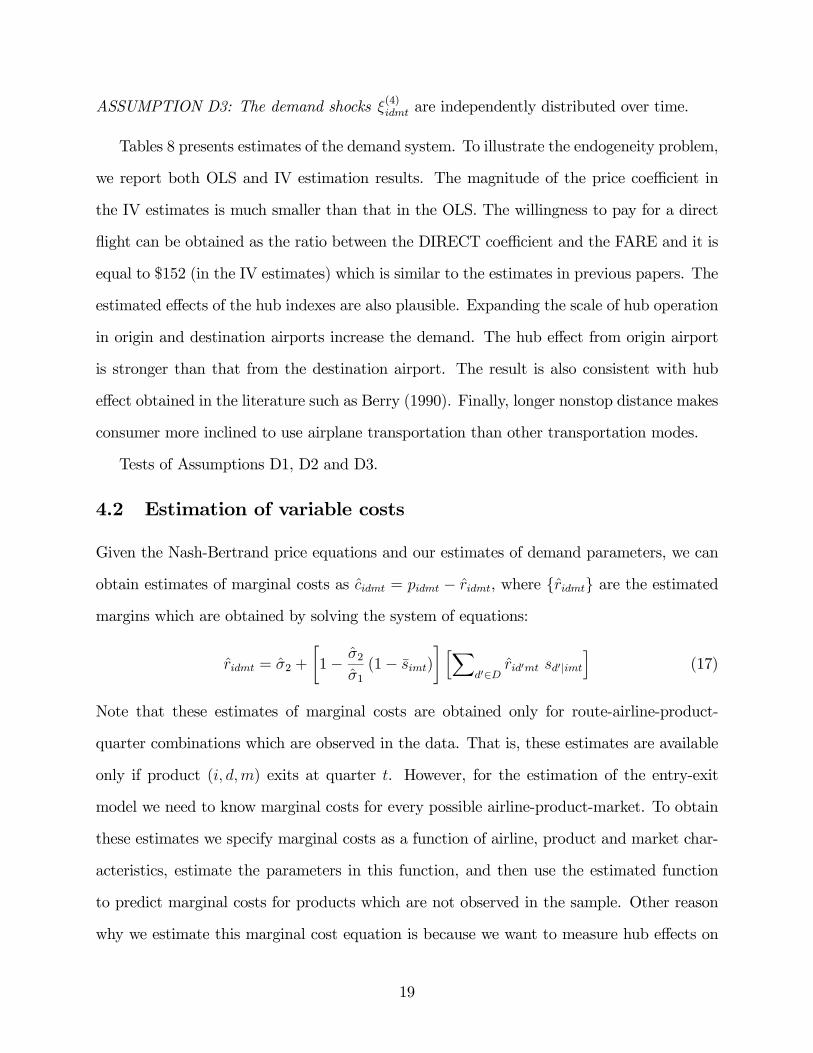
ASSUMPTION D3: The demand shocks ξ(4)idmt are independently distributed over time.

Tables 8 presents estimates of the demand system. To illustrate the endogeneity problem,

we report both OLS and IV estimation results. The magnitude of the price coefficient in

the IV estimates is much smaller than that in the OLS. The willingness to pay for a direct

flight can be obtained as the ratio between the DIRECT coefficient and the FARE and it is

equal to $152 (in the IV estimates) which is similar to the estimates in previous papers. The

estimated effects of the hub indexes are also plausible. Expanding the scale of hub operation

in origin and destination airports increase the demand. The hub effect from origin airport

is stronger than that from the destination airport. The result is also consistent with hub

effect obtained in the literature such as Berry (1990). Finally, longer nonstop distance makes

consumer more inclined to use airplane transportation than other transportation modes.

Tests of Assumptions D1, D2 and D3.

4.2 Estimation of variable costs

Given the Nash-Bertrand price equations and our estimates of demand parameters, we can

obtain estimates of marginal costs as cidmt = pidmt − ridmt, where {ridmt} are the estimated

margins which are obtained by solving the system of equations:

ridmt = σ2 +

∙1− σ2

σ1(1− simt)

¸ hXd0∈D

rid0mt sd0|imt

i(17)

Note that these estimates of marginal costs are obtained only for route-airline-product-

quarter combinations which are observed in the data. That is, these estimates are available

only if product (i, d,m) exits at quarter t. However, for the estimation of the entry-exit

model we need to know marginal costs for every possible airline-product-market. To obtain

these estimates we specify marginal costs as a function of airline, product and market char-

acteristics, estimate the parameters in this function, and then use the estimated function

to predict marginal costs for products which are not observed in the sample. Other reason

why we estimate this marginal cost equation is because we want to measure hub effects on

19

marginal costs. Our specification of the marginal cost function is very similar to the one of

the product qualities:

cidmt = δ1 dNS + δ2HUBO

im + δ3HUBDim + δ4DISTm + ω

(1)i + ω

(2)Omt + ω

(3)Dmt + ω

(4)idmt (18)

We make the following assumptions on the idiosyncratic shocks in marginal costs.

ASSUMPTION MC1: For any airline i and any two markets m 6= m0, the marginal cost

shocks ω(4)idmt and ω(4)idm0t are independently distributed.

ASSUMPTION MC2: The marginal cost shocks ω(4)idmt are independently distributed over

time.

Assumption MC1 implies that the hub size variables are exogenous regressors. Assumption

MC2 implies that ω(4)idmt is not a state variable in the entry-exit game and therefore there is

not self-selection bias in the estimation of the marginal cost function.

Table 9 presents OLS estimates of the marginal cost function. The marginal cost of a

direct flight is $12 larger than the marginal cost of an stop-flight, but this difference is not

statistically significant. Distance has a significantly positive effect on marginal cost. The

airline scale of operation (hub size) at the origin and destination airports reduce marginal

costs.

Tests of Assumptions MC1 and MC2.

Given our estimates of demand and marginal cost parameters we construct the following

estimates of cost-adjustment qualities for every possible tuple (i, d,m, t):

βidm =³β1 − δ1

´d+

³β2 − δ2

´HUBO

im +³β3 − δ3

´HUBD

im +³β4 − δ4

´DISTm

+³ξ(1)

i − ω(1)i

´+³ξ(2)

Om − ω(2)Om

´+³ξ(3)

Dm − ω(3)Dm

´(19)

20

4.3 Estimation of the dynamic entry-exit game

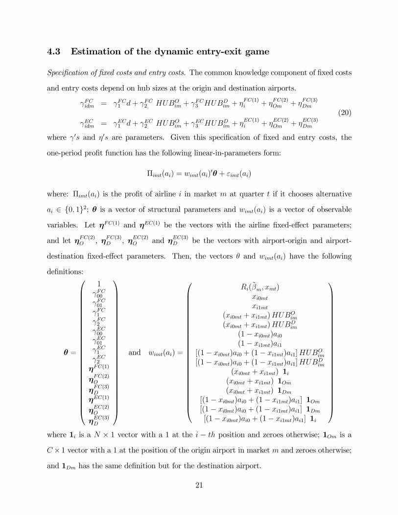
Specification of fixed costs and entry costs. The common knowledge component of fixed costs

and entry costs depend on hub sizes at the origin and destination airports.

γFCidm = γFC1 d+ γFC2 HUBOim + γFC3 HUBD

im + ηFC(1)i + η

FC(2)Om + η

FC(3)Dm

γECidm = γEC1 d+ γEC2 HUBOim + γEC3 HUBD

im + ηEC(1)i + η

EC(2)Om + η

EC(3)Dm

(20)

where γ0s and η0s are parameters. Given this specification of fixed and entry costs, the

one-period profit function has the following linear-in-parameters form:

Πimt(ai) = wimt(ai)0θ + εimt(ai)

where: Πimt(ai) is the profit of airline i in market m at quarter t if it chooses alternative

ai ∈ {0, 1}2; θ is a vector of structural parameters and wimt(ai) is a vector of observable

variables. Let ηFC(1) and ηEC(1) be the vectors with the airline fixed-effect parameters;

and let ηFC(2)O , ηFC(3)D , ηEC(2)O and ηEC(3)D be the vectors with airport-origin and airport-

destination fixed-effect parameters. Then, the vectors θ and wimt(ai) have the following

definitions:

θ =

⎛⎜⎜⎜⎜⎜⎜⎜⎜⎜⎜⎜⎜⎜⎜⎜⎜⎜⎜⎜⎜⎜⎜⎜⎜⎜⎝

1γFC00γFC01γFC1γFC2γEC00γEC01γEC1γEC2ηFC(1)

ηFC(2)O

ηFC(3)D

ηEC(1)

ηEC(2)O

ηEC(3)D

⎞⎟⎟⎟⎟⎟⎟⎟⎟⎟⎟⎟⎟⎟⎟⎟⎟⎟⎟⎟⎟⎟⎟⎟⎟⎟⎠

and wimt(ai) =

⎛⎜⎜⎜⎜⎜⎜⎜⎜⎜⎜⎜⎜⎜⎜⎜⎜⎜⎜⎜⎜⎜⎜⎜⎜⎝

Ri(βm, xmt)xi0mt

xi1mt

(xi0mt + xi1mt)HUBOim

(xi0mt + xi1mt)HUBDim

(1− xi0mt)ai0(1− xi1mt)ai1

[(1− xi0mt)ai0 + (1− xi1mt)ai1]HUBOim

[(1− xi0mt)ai0 + (1− xi1mt)ai1]HUBDim

(xi0mt + xi1mt) 1i(xi0mt + xi1mt) 1Om(xi0mt + xi1mt) 1Dm

[(1− xi0mt)ai0 + (1− xi1mt)ai1] 1Om[(1− xi0mt)ai0 + (1− xi1mt)ai1] 1Dm

[(1− xi0mt)ai0 + (1− xi1mt)ai1] 1i

⎞⎟⎟⎟⎟⎟⎟⎟⎟⎟⎟⎟⎟⎟⎟⎟⎟⎟⎟⎟⎟⎟⎟⎟⎟⎠where 1i is a N × 1 vector with a 1 at the i − th position and zeroes otherwise; 1Om is a

C×1 vector with a 1 at the position of the origin airport in market m and zeroes otherwise;

and 1Dm has the same definition but for the destination airport.

21

We assume that private information shocks {εimt(ai)} are iid Type 1 extreme value ran-

dom variables with dispersion parameter σε. Under these assumptions, the equilibrium

mapping in CCPs has the following form:

Ψimt(ai|P) =exp

©vPimt(ai)/σε

ªXa∗i∈{0,1}2

exp {vPimt(a∗i )/σε}

=

exp

½wPimt(ai)

0 θ

σε+ ePimt(ai)

¾X

a∗i∈{0,1}2exp

½wPimt(a

∗i )0 θ

σε+ ePimt(a

∗i )

¾(21)

wPimt(ai) is the expected and discounted value of current future vectors wi given that the

current state is (xmt, zm), that airline i choose alternative i and that all the firms behave

in the future according to their probabilities in P. Similarly, ePimt(ai) is the expected and

discounted value of eimt+s ≡ − lnPi(aimt+s|xmt+s, zm) given given that the current state is

(xmt, zm), that airline i choose alternative i and that all the firms behave in the future

according to their probabilities in P.

Nested Pseudo Likelihood (NPL) Estimator. For the sake of notational simplicity, let’s use

θ to represent θ/σε. For arbitrary values of θ and P, define the likelihood function:

Q(θ,P) ≡MX

m=1

TXt=1

NXi=1

lnΨimt(aimt|θ,P)

=MX

m=1

TXt=1

NXi=1

lnexp

©wPimt(aimt)

0θ + ePimt(aimt)ª

Xai∈{0,1}2

exp

½wPimt(ai)

0 θ

σε+ ePimt(ai)

¾ (22)

Let θ0 be the true value of the θ in the population, and let P0 be the true equilibrium CCPs

in the population. If the model is correct, then P0 is an equilibrium associated with θ0:

i.e., P0 = Ψ(θ0,P0). A two-step estimator of θ is defined as a pair (θ, P) such that P is a

nonparametric consistent estimator of P0 and θ maximizes the pseudo likelihood Q(θ, P).

The main advantage of this estimator is its simplicity. However, it has several important

limitations (see Aguirregabiria and Mira, 2007). In particular, it can be seriously biased

22

due to the imprecise nonparametric estimates of P. The NPL estimator is defined as a pair

(θ, P) that satisfies the following two conditions (Aguirregabiria and Mira, 2007):

θ = argmaxθ∈Θ

Q(θ, P)

P = Ψ(θ, P)

(23)

That is, θ maximizes the pseudo likelihood given P (as in the two-step estimator), and

P is an equilibrium associated with θ. This estimator has lower asymptotic variance and

finite sample bias than the two step estimator. A simple (though not necessarily efficient)

algorithm to obtain the NPL estimator is just a recursive extension of the two-step method.

We can start with an initial estimator of CCPs, say P0, not necessarily a consistent estimator

of P0, and then apply the following recursive procedure. At iteration K ≥ 1, we update our

estimates of (θ0,P0) by using the pseudo maximum likelihood estimator θK = argmaxθ∈Θ

Q(θ, PK−1) and then the policy iteration PK = Ψ(θK , PK−1), that is:

PK,imt(ai) =exp

nwPK−1imt (ai)

0θK + ePK−1imt (ai)

oX

a∗i∈{0,1}2exp

nwPK−1imt (a∗i )

0θK + ePK−1imt (a∗i )

o (24)

Upon convergence this algorithm provides the NPL estimator. Maximization of the pseudo

likelihood function with respect to θ is extremely simple because Q(θ,P) is globally concave

in θ for any possible value of P. The main computational burden in the implementation of

the NPL estimator comes from the calculation of the present values wPimt and ePimt. We now

describe in detail on the computation of these values.

Computing the present values wPimt and ePimt. Let fPxi(xmt+1|xmt, zm, aimt) be the transition

probability of the vector of incumbent status {xmt} conditional on the current choice of airline

i. This transition probability is a known function of the vector of CCPs P. It is possible

to show that (for notational simplicity I omit zm as an argument in CCPs, transitions and

23

values):

wPimt(ai) = wimt(ai) + δX

xmt+1∈{0,1}2NfPxi(xmt+1|xmt, ai) W

Piw(xmt+1)

ePimt(ai) = δX

xmt+1∈{0,1}2NfPxi(xmt+1|xmt, ai) W

Pie (xmt+1)

(25)

where WPiw(.) is a 1 × dim(θ) vector and WP

ie (.) is a scalar and both are (basis functions

for) valuation operators. Define the matrixWPi ≡ {[WP

iw(x),WPie (x)] : x ∈ {0, 1}2N}. Then,

the valuation basisWPi is defined as the unique solution inW to the following contraction

mapping:

W =X

ai∈{0,1}2Pi(ai) ∗

©[wi(ai),− lnPi(ai)]+δ F

Pxi(ai)W

ª(26)

where Pi(a) is the column vector of CCPs {Pi(ai|x) : ai ∈ {0, 1}2;x ∈ {0, 1}2N}. The com-

putational cost to obtain these values is equivalent to solving once the dynamic programming

(DP) of an airline. However, due to the relatively large number of heterogeneous players,

this DP problem has high dimensionality. The number of states x is 22∗27 ' 1016. It is clear

that solving this problem exactly would be extremely demanding.

We use interpolation-randomization in a very similar way as in Rust (1997) to approx-

imate WPi , w

Pimt(ai) and ePimt(ai). Let X

∗ = {x1, x2, ..., x|X∗|} be a subset of the actual

state space {0, 1}2N . The number of elements in this subset, |X∗|, is given by the amount

of high-speed memory in our computer. The grid points in X∗ can be selected by making

|X∗| random draws from a uniform distribution over the set {0, 1}2N . Define the following

transition probabilities:

fP∗xi (x0|x, ai) =

fPxi(x0|x, ai)P

x00∈X∗ fPxi(x

00|x, ai)(27)

And let FP∗xi (ai) be the matrices of transition probabilities associated with fP∗xi . Similarly,

we define P∗i (ai) and w∗i (ai) as Pi(ai) and wi(ai), respectively, but restricted to the set X∗.

Then, we can defineWP∗i as the unique solution inW to the following contraction mapping:

W =X

ai∈{0,1}2P∗i (ai) ∗

©[w∗i (ai),− lnP∗i (ai)] +δ FP∗xi (ai)W

ª(28)

24

GivenWP∗i , our approximation to the values w

Pimt(ai) and ePimt(ai) is:

wP∗imt(ai) = wimt(ai) + δX

xmt+1∈X∗fP∗xi (xmt+1|xmt, ai) W

P∗iw (xmt+1)

eP∗imt(ai) = δX

xmt+1∈X∗fP∗xi (xmt+1|xmt, ai) W

P∗ie (xmt+1)

(29)

As discussed in Rust (1997), this approximation has several interesting properties. In gen-

eral, these approximations are much more precise than the ones based on simple forward

simulations. For our estimates we have considered a set X∗ with 10, 000 cells which are

random draws from a uniform distribution.

Estimation results. Table 11 presents our estimation results for the entry-exit game. We

find very significant (both statistically and economically) hub-size effects in fixed operating

costs and in entry costs. The effects are particularly important for the case of entry costs.

Sunk entry costs are approximately twice the fixed operating costs of a quarter. *** More

discussion. Specification tests.

5 Disentangling demand, cost and strategic factors

We now use our estimate model to measure the contribution of demand, cost and strategic

factors to explain why most companies in the US airline industry operate using a hub-

spoke network. Define the hub− ratio of an airline as the fraction of passengers flying with

that airline who have to take a connecting flight in the hub airport of that airline.16 We

analyze how different hub-size effects contribute to the observe hub-ratio of different airlines.

The parameters that measure hub-size effects are: cots-adjusted qualities,³β2 − δ2

´and³

β3 − δ3´; fixed costs, γFC1 and γFC2 ; and entry-costs, γEC1 and γEC2 . For each of these

groups of parameters we perform the following experiments. We make the parameters (for

a single airline) equal to zero. Then, we calculate the new equilibrium, and obtain the value

of the hub-ratio for that airline.16In the calculation of this ratio we do not consider passengers whose flights have origin or destination in

the hub airport of the airline.

25

Let θ be the vector of structural parameters in the model. An equilibrium associated

with θ is a vector of choice probabilities P that solves the fixed point problem P = Ψ(θ,P).

For a given value θ, the model can have multiple equilibria. The model can be completed

with an equilibrium selection mechanism. This mechanism can be represented as a function

that, for given θ, selects one equilibrium within the set of multiple equilibria associated with

θ. We use π(θ) to represent this (unique) selected equilibrium. Our approach here (both

for the estimation and for counterfactual experiments) is completely agnostic with respect

to the equilibrium selection mechanism. We assume that there is such a mechanism, and

that it is a smooth function of θ. But we do not specify any specific equilibrium selection

mechanism π(.). Let θ0 be the true value of θ in the population under study. Suppose that

the data (and the population) come from a unique equilibrium associated with θ0. Let P0

be the equilibrium in the population. By definition, P0 is such that P0 = Ψ(θ0,P0) and

P0 = π(θ0). Suppose that given these data and assumptions we have a defined above a

consistent estimator of (θ0,P0). Let (θ0, P0) be this consistent estimator. Note that, even

after the estimation of the model, we do not know the function π(θ). All what we know

is that the point (θ0, P0) belongs to the graph of this function π. We want to use the

estimated model to study airlines’ behavior and equilibrium outcomes under counterfactual

scenarios which can be represented in terms of different values θ. Let θ∗ be the vector of

parameters under a counterfactual scenario. We want to know the counterfactual equilibrium

π(θ∗). The key issue to implement this experiment is that given θ∗ the model has multiple

equilibria, and we do not know the function π. We propose here a method to deal with this

problem. The method is based on the following assumptions for the equilibrium mapping

and the equilibrium selection mechanism.

Assumption: The mapping Ψ is continuously differentiable in (θ,P), and the equilibrium

selection mechanism π(θ) is a continuously differentiable function of θ around (θ0, P0).

Under this assumption we can use a first order Taylor expansion to obtain an approxima-

tion to the counterfactual choice probabilities π(θ∗) around our estimator θ0. An intuitive

26

interpretation of our approach is that we select the counterfactual equilibrium which is

"closer" (in a Taylor-approximation sense) to the equilibrium estimated from the data. The

data is not only used to identify the equilibrium in the population but also to identify the

equilibrium in the counterfactual experiments. Given the differentiability of the function

π(.) and of the equilibrium mapping, a Taylor approximation to π(θ∗) around our estimator

θ0 implies that:

π(θ∗) = π³θ0´+

∂π³θ0´

∂θ0

³θ∗ − θ0

´+O

µ°°°θ∗ − θ0°°°2¶ (30)

Note that π³θ0´= P0 and that π

³θ0´= Ψ

³θ0,π

³θ0´´. Differentiating this last expres-

sion with respect to θ we have that

∂π³θ0´

∂θ0=

∂Ψ³θ0,π

³θ0´´

∂θ0+

∂Ψ³θ0,π

³θ0´´

∂P0

∂π³θ0´

∂θ0(31)

And solving for ∂π³θ0´/∂θ0 we can represent this Jacobian matrix in terms of Jacobians

of Ψ evaluated at the estimated values (θ0, P0). That is,

∂π³θ0´

∂θ0=

ÃI − ∂Ψ(θ0, P0)

∂P0

!−1∂Ψ(θ0, P0)

∂θ0(32)

Solving expression (32) into (30) we have that:

π(θ∗) = P0 +

ÃI − ∂Ψ(θ0, P0)

∂P0

!−1∂Ψ(θ0, P0)

∂θ0

³θ∗ − θ0

´+O

µ°°°θ∗ − θ0°°°2¶ (33)

Therefore, under the condition that°°°θ∗ − θ0°°°2 is small, the term ³I − ∂Ψ(θ0,P0)

∂P0

´−1∂Ψ(θ0,P0)

∂θ0³θ∗ − θ0

´provides a good approximation to the counterfactual equilibriumπ(θ∗). Note that

all the elements in³I − ∂Ψ(θ0,P0)

∂P0

´−1∂Ψ(θ0,P0)

∂θ0

³θ∗ − θ0

´are known to the researcher. The

most attractive features of this approach are its simplicity and that it is quite agnostic about

the equilibrium selection.

Table 12 presents our estimates of the effects on the hub-ratio of eliminating hub-size

effects in cost-adjusted qualities, fixed costs and entry costs. For the moment we report

estimates only for two airlines: American and United. The most important effects come

27

from eliminating hub-size effects in entry costs. Furthermore, we find that strategic effects

are important.

6 Conclusions

To be written

28

References

[1] Aguirregabiria, V., and P. Mira (2007): “Sequential Estimation of Dynamic DiscreteGames,” Econometrica, 75, 1-53.

[2] Bailey, E., D. Graham, and D. Kaplan (1985): Deregulating the Airlines. Cambridge,Mass.: The MIT Press.

[3] Bajari, P., L. Benkard and J. Levin (2007): “Estimating Dynamic Models of ImperfectCompetition,” Econometrica, 75, 1331-1370.

[4] Berry, S. (1990): "Airport Presence as Product Differentiation," American EconomicReview, 80, 394-399.

[5] Berry, S. (1992): “Estimation of a model of entry in the airline industry”, Econometrica,60(4), 889-917.

[6] Berry, S. (1994): “Estimating Discrete-choice Models of Product Differentiation.”RAND Journal of Economics, 25, 242—262.

[7] Berry, S, J. Levinsohn, and A. Pakes (1995). “Automobile Prices in Market Equilib-rium.” Econometrica, 63, 841—890.

[8] Berry, S., M. Carnall, and P. Spiller (2006): “Airline Hubbing, Costs and Demand,” inAdvances in Airline Economics, Vol. 1: Competition Policy and Antitrust, D. Lee, ed.Elsevier Press.

[9] Boguslaski, C., H. Ito, and D. Lee (2004), "Entry Patterns in the Southwest AirlinesRoute System", Review of Industrial Organization 25(3), 317-350.

[10] Borenstein, S. (1989): “Hubs and high fares: Dominance and market power in the USairline industry”, Rand Journal of Economics, 20(3), 344-365.

[11] Borenstein, S. (1991), "The Dominant Firm-Advantage in Multiproduct Industries: Ev-idence from the U.S. Airlines", Quarterly Journal of Economics 106(4), 1237-1266.

[12] Borenstein, S. (1992): "The Evolution of U.S. Airline Competition." Journal of Eco-nomic Perspectives, Vol. 6.

[13] Bresnahan, T., and P. Reiss (1993): “Measuring the importance of sunk costs”, AnnalesD’Economie Et De Statistique, 31, 181-217.

[14] Cardell, S. (1997): "Variance components structures for the extreme-value and logisticdistributions with application to models of heterogeneity ," Econometric Theory, 13,185-213.

29

[15] Caves, D., L. Christensen, and M. Tretheway (1984): “Economies of Density versusEconomies of Scale: Why Trunk and Local Service Airline Costs Differ,” The RANDJournal of Economics, 15 (4), 471-489.

[16] Ciliberto, F. and E. Tamer (2006): "Market structure and multiple equilibria in airlinemarkets," manuscript, University of Virginia.

[17] Doraszelski, U., and Satterthwaite, M. (2003): ”Foundations of Markov-perfect industrydynamics: Existence, purification, and multiplicity,”Working paper, Hoover Institution,Stanford.

[18] Ericson, R., and A. Pakes (1995): “Markov-Perfect industry dynamics: A frameworkfor empirical work”, Review of Economic Studies, 62, 53-82.

[19] Evans, W.N. and I. N. Kessides (1993), “Localized Market Power in the U.S. AirlineIndustry,” The Review of Economics and Statistics, 75 (1), 66-68.

[20] Gayle, K. (2004): "Does Price Matter? Price or Non-Price Competition in the AirlineIndustry ," manuscript, Department of Economics, Kansas State University.

[21] Hendricks, K., M. Piccione, and G. Tan (1995): "The Economics of Hubs: The Case ofMonopoly," The Review of Economic Studies, 62(1), 83-99.

[22] Hendricks, K., M. Piccione, and G. Tan (1997): “Entry and exit in hub-spoke networks,”Rand Journal of Economics, 28(2), 291—303.

[23] Ito, H. and D. Lee (2004): “Incumbent Reponses to Lower Cost Entry: Evidence fromthe U.S. Airline Industry,” manuscript.

[24] Januszewski, J (2004): "The Effect of Air Traffic Delays on Airline Prices," manuscript,Department of Economics, UC San Diego.

[25] Januszewski, J. and M. Lederman (2003): "Entry Patterns of Low-Cost Airlines ,"manuscript, Rotman School of Management, University of Toronto.

[26] Judd, K. (1985): "Credible Spatial Preemption," The RAND Journal of Economics,16(2), 153-166.

[27] Kahn, A. (2004): Lessons from Deregulation: Telecommunications and Airlines Afterthe Crunch, Washington, DC: AEI-Brookings Joint Center for Regulatory Studies.

[28] Lederman, M. (2004): "Do Enhancements to Loyalty Programs Affect Demand? TheImpact of International Frequent Flyer Partnerships on Domestic Airline Demand ,"manuscript, Rotman School of Management, University of Toronto.

30

[29] Morrison, S. A. and C. Winston, (1986): The Economic Effects of Airline Deregulation,Brookings, Washington, D. C.

[30] Transportation Research Board (1999): "Entry and Competition in the U.S. AirlineIndustry: Issues and Opportunities," National Research Council, Special Report 255,Washington, D.C.

[31] Morrison, S. A. and C. Winston, (1995): The Evolution of the Airline Industry, Brook-ings, Washington, D.C.

[32] Morrison, S. A., and C. Winston. (2000): "The remaining role for government policy inthe deregulated airline industry," in Deregulation of network industries: What’s next?,edited by Sam Peltzman and Clifford Winston. Washington, DC: AEI-Brookings JointCenter for Regulatory Studies.

[33] Oum, T., A. Zhang, and Y. Zhang (1995): "Airline Network Rivalry," Canadian Journalof Economics, 28, 836-857.

[34] Pakes, A. and P. McGuire (1994): “Computing Markov-Perfect Nash equilibria: Numer-ical implications of a dynamic differentiated product model, Rand Journal of Economics,555-589.

[35] Pakes, A., M. Ostrovsky, and S. Berry (2007): “Simple estimators for the parameters ofdiscrete dynamic games (with entry/exit examples),” manuscript, Harvard University.

[36] Pesendorfer, M. and Schmidt-Dengler (2007): “Asymptotic Least Squares Estimatorsfor Dynamic Games," forthcoming in The Review of Economic Studies.

[37] Reiss, P.C. and P.T. Spiller (1989), "Competition and Entry in Small Airline Markets",Journal of Law and Economics 32, S179-S202.

[38] Rust, J. (1997): "Using Randomization to Break the Curse of Dimensionality," Econo-metrica, 65, 487-516.

[39] Sinclair, R.A. (1995), "An Empirical Model of Entry and Exit in Airline Markets",Review of Industrial Organization 10, 541-557.

31

Table 1Cities (or Metropolitan Areas), Airports and Population

City, State Airports City Pop. City, State Airports City Pop.

New York-Newark-Jersey LGA, JFK, EWR 8,623,609 Las Vegas, NV LAS 534,847

Los Angeles, CA LAX, BUR 3,845,541 Portland, OR PDX 533,492

Chicago, IL ORD, MDW 2,862,244 Oklahoma City, OK OKC 528,042

Dallas, TX(1) DAL, DFW 2,418,608 Tucson, AZ TUS 512,023

Phoenix-Tempe-Mesa, AZ PHX 2,091,086 Albuquerque, NM ABQ 484,246

Houston, TX HOU, IAH, EFD 2,012,626 Long Beach, CA LGB 475,782

Philadelphia, PA PHL 1,470,151 New Orleans, LA MSY 462,269

San Diego, CA SAN 1,263,756 Cleveland, OH CLE 458,684

San Antonio,TX SAT 1,236,249 Sacramento, CA SMF 454,330

San Jose, CA SJC 904,522 Kansas City, MO MCI 444,387

Detroit, MI DTW 900,198 Atlanta, GA ATL 419,122

Denver-Aurora, CO DEN 848,678 Omaha, NE OMA 409,416

Indianapolis, IN IND 784,242 Oakland, CA OAK 397,976

Jacksonville, FL JAX 777,704 Tulsa, OK TUL 383,764

San Francisco, CA SFO 744,230 Miami, FL MIA 379,724

Columbus, OH CMH 730,008 Colorado Spr, CO COS 369,363

Austin, TX AUS 681,804 Wichita, KS ICT 353,823

Memphis, TN MEM 671,929 St Louis, MO STL 343,279

Minneapolis-St. Paul, MN MSP 650,906 Santa Ana, CA SNA 342,715

Baltimore, MD BWI 636,251 Raleigh-Durham, NC RDU 326,653

Charlotte, NC CLT 594,359 Pittsburg, PA PIT 322,450

El Paso, TX ELP 592,099 Tampa, FL TPA 321,772

Milwaukee, WI MKE 583,624 Cincinnati, OH CVG 314,154

Seattle, WA SEA 571,480 Ontario, CA ONT 288,384

Boston, MA BOS 569,165 Buffalo, NY BUF 282,864

Louisville, KY SDF 556,332 Lexington, KY LEX 266,358

Washington, DC DCA, IAD 553,523 Norfolk, VA ORF 236,587

Nashville, TN BNA 546,719

Note (1): Dallas-Arlington-Fort Worth-Plano, TX

32

Table 2Top Routes (Rountrip) in 2004

ORIGIN CITY DESTINATION CITY # Passengers

(Annual, Rountrip)

1. New York Chicago 782,420

2. Chicago New York 759,950

3. Chicago Las Vegas 748,310

4. New York Las Vegas 740,440

5. Los Angeles Las Vegas 739,810

6. Los Angeles New York 735,180

7. New York Los Angeles 685,190

8. Atlanta New York 645,680

9. New York Atlanta 595,630

10. Oakland Los Angeles 556,010

11. Los Angeles Oakland 540,000

12. New York San Francisco 509,240

13. Chicago Los Angeles 479,060

14. New York Miami 478,940

15. San Francisco New York 464,510

16. Los Angeles Chicago 464,300

17. New York Tampa 448,770

18. Chicago Phoenix 438,880

19. Dallas Houston 419,360

20. Dallas New York 391,220

21. Houston Dallas 380,470

22. Boston New York 369,250

23. Phoenix Las Vegas 363,300

24. New York Boston 360,240

25. New York Washington 360,110

Source: DB1B Database

\

33

Table 3Airlines

Airline (Code) # Passengers(1) # Markets(2)

(in thousands) 2004-Q4

1. Southwest (WN) 25,026 975

2. American (AA)(3) 20,064 1,464

3. United (UA)(4) 15,851 1,142

4. Delta (DL)(5) 14,402 1,280

5. Continental (CO)(6) 10,084 689

6. Northwest (NW)(7) 9,517 822

7. US Airways (US) 7,515 555

8. America West (HP)(8) 6,745 585

9. Alaska (AS) 3,886 73

10. ATA (TZ) 2,608 152

11. JetBlue (B6) 2,458 45

12. Frontier (F9) 2,220 176

13. AirTran (FL) 2,090 199

14. Mesa (YV)(9) 1,554 260

15. Midwest (YX) 1,081 76

16. Trans States (AX) 541 63

17. Reno Air (QX) 528 59

18. Spirit (NK) 498 16

19. Sun Country (SY) 366 21

20. PSA (16) 84 48

21. Ryan International (RD) 78 3

22. Allegiant (G4) 67 5

23. Aloha (AQ) 44 8

Note (1): Annual number of passengers in 2004 for our

selected markets.

Note (2): We consider that airline is active in a market if

it has at last 20 passengers per week.

Note (3): American (AA) + American Eagle (MQ) + Executive (OW)

Note (4): United (UA) + Air Wisconsin (ZW)

Note (5): Delta (DL) + Comair (OH) +Atlantic Southwest (EV)

Note (6): Continental (CO) + Expressjet (RU)

Note (7): Northwest (NW) + Mesaba (XJ)

Note (8): On 2005, America West merged with US Airways.Note (9): Mesa (YV) + Freedom (F8)

34

Table 4Airlines and Hub Size (2004-Q4)

Airline (Code) Largest Hub Second largest Hub

(people in millions) (people in millions)

1. Southwest (WN) MCI (31.5) BWI (30.5)2. American (AA) DFW (46.7) ORD (44.4)|3. United (UA) DEN (45.9) SFO (45.8)4. Delta (DL) ATL (48.5) TPA (46.8)5. Continental (CO) IAH (46.9) CLE (45.6)6. Northwest (NW) DTW (47.6) MSP (47.1)7. US Airways (US) CLT (39.2) BOS (38.6)8. America West (HP) PHX (39.6) LAS (36.1)9. Alaska (AS) SEA (29.0) PDX (26.0)10. ATA (TZ) IND (26.2) MDW (25.0)11. JetBlue (B6) LGB (10.7) OAK (10.2)12. Frontier (F9) DEN (35.1) PDX (14.2)13. AirTran (FL) ATL (30.7) MEM (25.4)14. Mesa (YV) AUS (23.1) BNA (22.2)15. Midwest (YX) MKE (29.9) MCI (14.6)16. Trans States (AX) STL (25.4) PIT (12.6)17. Reno Air (QX) PDX (25.9) OMA (10.7)18. Spirit (NK) DTW (13.9) LAX (12.4)19. Sun Country (SY) MSP (21.6) JFK (0.6)20. PSA (16) ATL (10.0) IND (8.9)21. Ryan International (RD) ATL (4.4) LAX (0.4)22. Allegiant (G4) LAS (0.7) OKC (0.5)23. Aloha (AQ) LAS (4.2)

35

Table 5Descriptive Statistics of Market Structure2,970 markets. Period 2004-Q1 to 2004-Q4

2004-Q1 2004-Q2 2004-Q3 2004-Q4 All Quarters

Markets with 0 airlines 7.27% 11.48 % 11.68% 11.75% 10.55 %Markets with 1 airline 13.06% 17.17% 17.21% 17.34% 16.20%Markets with 2 airlines 14.71% 18.89% 18.38% 19.33% 17.83%Markets with 3 airlines 15.93% 17.10 % 16.40% 16.33% 16.44%Markets with 4 airlines 15.82% 12.86% 14.14% 13.57% 14.10%

Markets with more than 4 airlines 33.20 % 22.49% 22.19% 21.68% 24.89%

Herfindahl Index (median) 4650 4957 4859 5000 4832

Distribution of Monopoly Markets:

Delta 15.13% 17.65% 15.26% 15.61% 15.96%American 14.87% 14.12% 15.07% 12.33% 14.04%Northwest 13.85% 13.33% 12.72% 14.45% 13.58%United 11.28% 12.35% 14.68% 15.22% 13.52%

Continental 9.23% 10.78% 13.31% 11.56 % 11.35%US Airways 8.72% 6.47% 4.89% 5.39% 6.22%Southwest 3.33% 7.84% 6.46% 4.62% 5.70%

Distribution of # Entrants:

Markets with 0 - 86.23% 73.91% 74.98% 78.37%Markets with 1 - 12.26% 21.48% 20.30% 18.01%Markets with 2 - 1.38% 4.14% 4.41% 3.31%

Markets with >2 - 0.13% 0.47% 0.30% 0.30%

Distribution of # Exits:

Markets with 0 - 49.29% 75.62% 71.72% 65.54%Markets with 1 - 31.58% 20.24% 22.26% 24.69%Markets with 2 - 12.05% 3.54% 5.08% 6.89%

Markets with >2 - 7.07% 0.61% 0.94% 2.87%

36

Table 6Transition Probability of Market Structure (Quarter 2 to 3)

# Firms in Q3# Firms in Q2 0 1 2 3 4 >4 Total

0 86.26% 11.40% 2.34% 0.00% 0.00% 0.00% 100.00%

1 8.27% 73.62% 15.55% 2.56% 0.00% 0.00% 100.00%

2 1.42% 13.48% 59.93% 20.04% 4.26% 0.89% 100.00%

3 0.20% 3.76% 20.20% 52.28% 19.21% 4.36% 100.00%

4 0.00% 0.79% 4.19% 21.20% 54.19% 19.63% 100.00%

>4 0.00% 0.00% 0.30% 2.69% 13.90% 83.11% 100.00%

37

Table 8Demand Estimation(1)

Data: 85,497 observations. 2004-Q1 to 2004-Q4OLS IV

FARE ($100) -0.329 (0.005) -1.366 (0.110)

ln(si|d) 0.500 (0.003) 0.113 (0.051)

DIRECT 1.217 (0.051) 2.080 (0.184)

HUBSIZE-ORIGIN 0.032 (0.001) 0.027 (0.002)

HUBSIZE-DESTINATION 0.041 (0.001) 0.036 (0.002)

DISTANCE 0.098 (0.002) 0.329 (0.013)

(1) All the estimations include airline dummies, origin-airport dummies × time dummies,

and destination-airport dummies × time dummies. Stadard errors in parentheses.

Table 9Marginal Cost Estimation(1)

Data: 85,497 observations. 2004-Q1 to 2004-Q4Dep. Variable: Marginal Cost in $100

Estimate (Std. Error)

DIRECT 0.012 (0.011)

HUBSIZE-ORIGIN -0.073 (0.012)

HUBSIZE-DESTINATION -0.036 (0.013)

DISTANCE 5.355 (0.012)

(1) All the estimations include airline dummies, origin-airport

dummies × time dummies, and destination-airport

dummies × time dummies.

38

Table 11Estimation of Dynamic Game of Entry-Exit(1)

Data: 4,970 markets × 27 airlines × 3 quarters = 402,570 observations

Estimate (Std. Error)(in million $)

Fixed Costs:γFC00 (stop-flight) 0.571 (0.006)

γFC01 (direct-flight) 0.620 (0.006)

γFC1 (hubsize origin) -0.036 (0.005)

γFC1 (hubsize destination) -0.022 (0.005)

Entry Costs:γEC00 (stop-flight) 0.977 (0.015)

γEC01 (direct-flight) 1.004 (0.016)

γEC1 (hubsize origin) -0.306 (0.018)

γEC1 (hubsize destination) -0.272 (0.020)

σε 0.316 (0.015)

(1) All the estimations include airline dummies, origin-airport dummies,

and destination-airport dummies. Stadard errors in parentheses.

Table 12Effects of Different Parameters on an Airline Hub-Ratio

Hub-RatiosNo hub-size effects No hub-size effects No hub-size effectsin variable profits in fixed costs in entry costs

Carrier Observed No Strat. Strategic No Strat. Strategic No Strat. Strategic

American 78.9 75.2 73.1 71.9 68.6 47.2 35.5

United 81.2 78.8 74.9 70.4 66.0 42.1 30.7

39